Part III Static Games of Incomplete Informationfaculty.haas.berkeley.edu/stadelis/Game...
40
Part III Static Games of Incomplete Information
-
Upload
duongnguyet -
Category
Documents
-
view
214 -
download
0
Transcript of Part III Static Games of Incomplete Informationfaculty.haas.berkeley.edu/stadelis/Game...
Part III
Static Games of Incomplete
Information
166

167
As we have seen so far the basic structure of a game, be it in normal form or
extensive form, proved useful in providing a formal structure to which we can apply
the game-theoretic solution concept of our choice. If it is a variant of the Prisoner’s
dilemma, we feel comfortable predicting static Nash equilibrium behavior, and in
dynamic settings we have explored the merits of requiring credible, sequentially
rational strategies for the players.
In all the examples, and appropriate tools for analysis, we have made an impor-
tant assumption: that the game played is common knowledge. In particular, we
have assumed that the players are aware of who is playing, what the possible ac-
tions of each player are, and how outcomes translate into payoffs. Furthermore, we
have assumed that this knowledge of the game is itself common knowledge, which
gave us the methodological foundation to develop such solution concepts as iter-
ated elimination of dominated strategies, rationalizability, and most importantly,
Nash equilibrium and Subgame Perfect equilibrium.
Little effort is needed to convince any experienced person that these ideal situa-
tions are not able to capture many interesting strategic interactions. Let’s consider
one of our first examples, the duopoly market structure. We have analyzed both
the Cournot and the Bertrand models of duopolistic behavior, and for each we have
a clear and precise, easily understood outcome. One assumption we made is that
the payoffs of the firms, like their action spaces, are common knowledge. However,
is it reasonable to assume that the production technologies are indeed common
knowledge? And if they are, should we believe that the efficiency of workers in
each form are known to the other firm? And more generally, that the cost function
of each firm is known to their opponent?
Clearly, it is more convincing to think that firm’s have a good idea about their
opponents costs, but do not know exactly what they are. Similarly, if one thinks of
a reasonable variant to the prisoner’s dilemma, I may not know how much honor
my fellow accomplice has, and whether he will be willing to rat on me for the sake
of getting a reduced sentence? And whether my partner in the battle-of-the-sexes
game really likes football games or the opera?
Yet, as realistic as these examples are, the tool-box we have developed so far
is not adequate to address these situations. How do we think situations in which

168
players have some idea about their opponents’ characteristics, but don’t know
them exactly? A careful thought might lead you to see that this is not so different
than the situation in a simultaneous move game: a player does not know what
action his opponents are taking, but he has to form an idea in order to choose
his best response, and we identified this idea as the player’s belief. Furthermore,
we developed our tools of analysis that required these beliefs, and the appropriate
best responses, to be consistent, which we called equilibrium.
As it turns out, in the mid 1960’s John Harsanyi not only realized this similarity,
but developed a very elegant, and extremely operational way to capture the ideas
of beliefs over not only the action’s of one’s opponents, but also over their other
characteristics, or their types, which led him to be the third Nobel laureate to
share the prestigious prize with John n Nash and Reinhard Selten in 1994. We call
games that incorporate the possibility that players may have different types games
of incomplete information.
Like with games of complete information, we must require these beliefs to be
consistent in order to develop some notion of equilibrium analysis. This is done,
following Harsanyi’s developments, by making a very strong assuming about the
intelligence of our players: we assume that common knowledge reigns over the
possible types of players, and over the likelihood that each type prevails.

This is page 1
Printer: Opaq
17
Incomplete Information: The Ideas
As before, we have the two “physical” components of a game, which are:
• N = {1, 2, ..., n} is the set of players
• Ai, i ∈ N, are the actions spaces for each player.
Thus, we are considering an n-player simultaneous-move game. However, the
distinction is that Instead of having a single utility function for each player that
maps profiles of actions into payoffs (which we had in games of complete informa-
tion), games of incomplete information will allow players to have one of possibly
many utility functions, thus capturing the idea that players’ preferences may not
be common knowledge.
To capture this idea we assume that first, before the game is played, Nature
chooses the preferences, or types of the different players.1 A way of thinking about
this methodology is that first, Nature chooses one of many games, and then the
game is played. Clearly, if Nature is randomly choosing between one of many
1As we will see soon, two different types of a player may not necessarily differ in that player’s preferences,
but may differ in knowledge that the player has about differences in preferences of other players. Since this is
a bit more subtle, we leave it for later, when we are more comfortable with the notion of Bayesian games and
incomplete information.
170 17. Incomplete Information: The Ideas
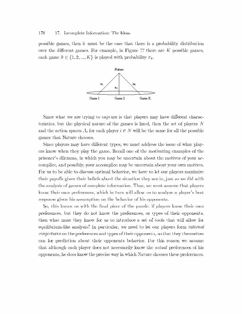
possible games, then it must be the case that there is a probability distribution
over the different games. For example, in Figure ?? there are K possible games,
each game k ∈ {1, 2, ...,K} is played with probability πk.
Since what we are trying to capture is that players may have different charac-
teristics, but the physical nature of the games is fixed, then the set of players N
and the action spaces Ai for each player i ∈ N will be the same for all the possible
games that Nature chooses.
Since players may have different types, we must address the issue of what play-
ers know when they play the game. Recall one of the motivating examples of the
prisoner’s dilemma, in which you may be uncertain about the motives of your ac-
complice, and possibly, your accomplice may be uncertain about your own motives.
For us to be able to discuss optimal behavior, we have to let our players maximize
their payoffs given their beliefs about the situation they are in, just as we did with
the analysis of games of complete information. Thus, we must assume that players
know their own preferences, which in turn will allow us to analyze a player’s best
response given his assumption on the behavior of his opponents.
So, this leaves us with the final piece of the puzzle: if players know their own
preferences, but they do not know the preferences, or types of their opponents,
then what must they know for us to introduce a set of tools that will allow for
equilibrium-like analysis? In particular, we need to let our players form rational
conjectures on the preferences and types of their opponents, so that they themselves
can for prediction about their opponents behavior. For this reason we assume
that although each player does not necessarily know the actual preferences of his
opponents, he does know the precise way in which Nature chooses these preferences.
17. Incomplete Information: The Ideas 171
That is, each player knows the probability distribution over types, and this itself
is common knowledge among the players of the game.
Thus, we have complemented the physical components, payoffs and action spaces,
with preferences and information components as follows:
• Nature: a probability distribution over types of players.
• Each player knows his type but not the other players’ types.
• The probability distribution over types is common knowledge.
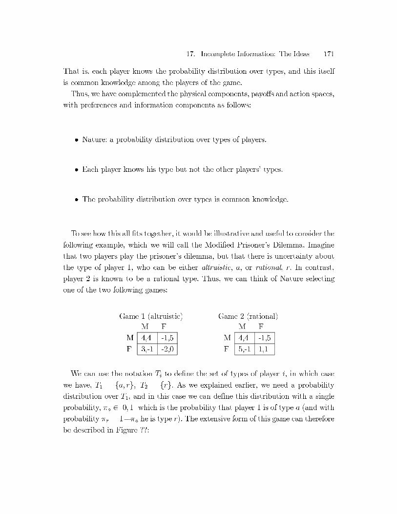
To see how this all fits together, it would be illustrative and useful to consider the
following example, which we will call the Modified Prisoner’s Dilemma. Imagine
that two players play the prisoner’s dilemma, but that there is uncertainty about
the type of player 1, who can be either altruistic, a, or rational, r. In contrast,
player 2 is known to be a rational type. Thus, we can think of Nature selecting
one of the two following games:
Game 1 (altruistic) Game 2 (rational)
M F
M 4,4 -1,5
F 3,-1 -2,0
M F
M 4,4 -1,5
F 5,-1 1,1
We can use the notation Ti to define the set of types of player i, in which case
we have, T1 = {a, r}, T2 = {r}. As we explained earlier, we need a probability
distribution over T1, and in this case we can define this distribution with a single
probability, πa ∈ [0, 1] which is the probability that player 1 is of type a (and with
probability πr = 1−πa he is type r). The extensive form of this game can therefore
be described in Figure ??:
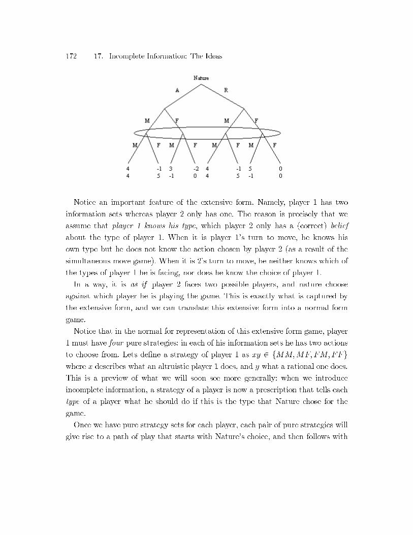
172 17. Incomplete Information: The Ideas
Notice an important feature of the extensive form. Namely, player 1 has two
information sets whereas player 2 only has one. The reason is precisely that we
assume that player 1 knows his type, which player 2 only has a (correct) belief
about the type of player 1. When it is player 1’s turn to move, he knows his
own type but he does not know the action chosen by player 2 (as a result of the
simultaneous move game). When it is 2’s turn to move, he neither knows which of
the types of player 1 he is facing, nor does he know the choice of player 1.
In a way, it is as if player 2 faces two possible players, and nature choose
against which player he is playing the game. This is exactly what is captured by
the extensive form, and we can translate this extensive form into a normal form
game.
Notice that in the normal for representation of this extensive form game, player
1 must have four pure strategies: in each of his information sets he has two actions
to choose from. Lets define a strategy of player 1 as xy ∈ {MM,MF,FM,FF}
where x describes what an altruistic player 1 does, and y what a rational one does.
This is a preview of what we will soon see more generally: when we introduce
incomplete information, a strategy of a player is now a prescription that tells each
type of a player what he should do if this is the type that Nature chose for the
game.
Once we have pure strategy sets for each player, each pair of pure strategies will
give rise to a path of play that starts with Nature’s choice, and then follows with
17. Incomplete Information: The Ideas 173
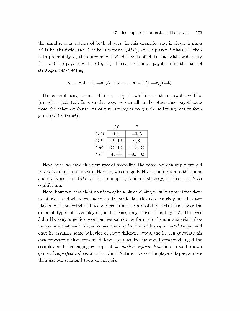
the simultaneous actions of both players. In this example, say, if player 1 plays
M is he altruistic, and F if he is rational (MF ), and if player 2 plays M , then
with probability πa the outcome will yield payoffs of (4, 4), and with probability
(1 − πa) the payoffs will be (5,−1). Thus, the pair of payoffs from the pair of
strategies (MF,M ) is,
u1 = πa4 + (1− πa)5, and u2 = πa4 + (1 − πa)(−1).
For concreteness, assume that πa = 1
2, in which case these payoffs will be
(u1, u2) = (4.5, 1.5). In a similar way, we can fill in the other nine payoff pairs
from the other combinations of pure strategies to get the following matrix form
game (verify these!):
M F
MM 4, 4 −1, 5
MF 4.5, 1.5 0,3
FM 3.5, 1.5 −1.5, 2.5
FF 4,−1 −0.5, 0.5
Now, once we have this new way of modelling the game, we can apply our old
tools of equilibrium analysis. Namely, we can apply Nash equilibrium to this game
and easily see that (MF,F ) is the unique (dominant strategy, in this case) Nash
equilibrium.
Note, however, that right now it may be a bit confusing to fully appreciate where
we started, and where we ended up. In particular, this new matrix games has two
players with expected utilities derived from the probability distribution over the
different types of each player (in this case, only player 1 had types). This was
John Harsanyi’s genius solution: we cannot perform equilibrium analysis unless
we assume that each player knows the distribution of his opponents’ types, and
once he assumes some behavior of these different types, the he can calculate his
own expected utility from his different actions. In this way, Harsanyi changed the
complex and challenging concept of incomplete information, into a well known
game of imperfect information, in which Nature chooses the players’ types, and we
then use our standard tools of analysis.

174 17. Incomplete Information: The Ideas
There is a potentially confusing point that is worth clarifying before we go on to
the more generalized and formal definitions. We can see how each type of player
i, say, having beliefs about the other players’ types and actions, can calculate his
expected utility. But by aggregating the types of all the types of each player into
some “meta” player (e.g., player 1 in the example), are we not going a bit too far?
Why will this player’s optimal response also be the optimal response of each of the
different types from which he is composed? This is precisely where the definitions
of strategies comes in. When player 1 in the combined matrix game chooses the
strategyMM , for example, then the rational type of player 1 is playing a dominated
strategy, M instead of F , but the altruistic type is playing his dominant strategy,
M . This is precisely why MF in the combined matrix game is better than MM :
it gives one type higher payoffs, and thus gives the “meta” player higher expected
payoffs. Once again, an elegant part of Harsanyi’s solution.
Since we are now finishing up with the ideas of this chapter, and will soon move
on to the more general definitions and applications, there is an important note
worth thinking about. Harsanyi’s elegant solution to the problem of incomplete
information is not something that we get for free. We are taking a big leap of faith
by assuming that the distribution of types, in the example above given by πaand
πr, are common knowledge. This is a step beyond the assumptions we made for
Nash Equilibrium, where we required players to form conjectures, or beliefs, that
in equilibrium have to match the choices of their opponents. Here we are asking for
more: all the players agree on the way in which players’ types differ from each other,
and on the way that Nature chooses among these profiles of types. The alternative
approach is not to assume this, and to forgo equilibrium analysis. Thus, when we
apply our models and tools to realistic situations, we should be mindful of the
strong informational assumptions we are making, which should guide us in putting
confidence in our predictions or prescriptions.
L13
This is page 1
Printer: Opaq
18
Normal form Representation of Static Bayesian
Games
18.1 Players, Actions, Information and Preferences
Recall that we represented a normal form game of complete information in chapter
2 by 〈N, {Si}n
i=1, {ui(·)}
n
i=1〉 where N = {1, 2, ..., n} is the set of players, Si is the
action, or strategy space of player i, and ui : S → � is the utility (payoff) function
of player i where S ≡ S1 × S2 × · · · × Sn.
Now we want to capture the fact that players know their own payoffs from
different actions, but that they do not know the payoffs of other players. For this
we introduced three new ideas. First, we said that before the game is actually
played, Nature chooses types for the different players, where each type can be
the information that the player has about his own payoffs, or more generally,
information he might have about other relevant attributes of the game. Thus, we
introduce type spaces for each player which represent the sets from which nature
chooses these types.
To capture the idea that there is common knowledge about the way in which
nature chooses between profiles of types of players, we introduce the notion of a
common prior, which is the commonly known probability distribution over types.
That is, every agent knows his own type, and he uses this prior to form posterior
beliefs over the types of other agents. Thus we get:

176 18. Normal form Representation of Static Bayesian Games
Definition: The normal form representation of an n-player static Bayesian game
is
〈N, {Ai}n
i=1, {Ti}
n
i=1, {ui(· ; ti), ti ∈ Ti}
n
i=1, {pi}
n
i=1〉
where N = {1, 2, ..., n} is the set of players, Ai is the action set of player i,
Ti = {t1i, t2
i, ..., t
ki
i} is the type space of player i, ui(·; ti) : A× Ti → � is the type
dependent utility function of player i, where A ≡ A1 × A2 × · · · × An , and pi
describes the belief of player i with respect to the uncertainty over the other
players’ types, that is pi(t−i|ti) is the (posterior) conditional distribution on
t−i (all other types but i) given that i knows his type is ti.
We assume that the timing of the game is as follows:
1. Nature chooses a profile of types.
2. Each player learns his own type and uses pi to form beliefs over the other
types.
3. Players simultaneously (therefore, static game) choose actions from there sets
Ai, i ∈ N .
4. payoffs ui(a1, a2, ..., an; ti) are realized for each player.
Note that in our setup we have player’s utility ui(·; ti) not depend on t−i, which
means that one player’s payoff does not depend on the types of the other players.
We call this setup private values, since each type’s payoff depends only on his
private information. This setup will not capture all the interesting examples we
will analyze, and for this reason we will later discuss the case of common values
where ui(a1, a2, ..., an; t1, t2, ..., tn) is allowed for. Yet, for expositional clarity, let’s
deal with the simpler case first.
18.2 Deriving Posteriors from a Common Prior: A Player’s Beliefs
In the definition of a Bayesian game we introduced the idea of a common prior,
that is, the distribution over the choices made by Nature. What does it mean for

18.2 Deriving Posteriors from a Common Prior: A Player’s Beliefs 177
player to use the common prior, and once he knows his type derive a posterior
belief about the distribution of the other players’ types? This is, not surprisingly,
just a simple application of Bayes’ rule.
The essence of Bayes’ rule is to provide a consistent mathematical rule that
derives the way in which you should change your initial (prior) beliefs in the light
of new evidence, resulting in a posterior belief. In our application, it allows a
player who does not know his type, but knows the initial distribution of all types
including his own, to derive new beliefs once he learns his type, and have these
beliefs consistent with the prior.
Formally, imagine that there are two of many possible states, S (say, it will be
sunny) and H (say, the waves will be high), that can occur exclusively or together
according to some prior distribution p(·). That is, p(·) describes the probabilities
assigned to any combination of these states being true. Let p(S) be the prior
probability that it will be sunny, p(H) be the prior probability that the waves will
be high, and p(S ∩H) be the prior probability that it will be both sunny and the
waves will be high. Let’s imagine that you wake up, and see that it is sunny; what
can you infer about the probability that the waves are high? It is not necessarily
true that it is p(H), because you just learned that it is sunny, and this is new
information. this is where Bayes rule comes in handy. It precisely tells you what is
the probability of state H given that you know state S happened, and is given by:
Pr{H |S} =p(S ∩H)
p(S)
The intuition works as follows. If we know that S occurred, there are now two
possibilities: either H occurred or not. Thus, we can think of two states: the first
being that both S and H occurred, which happens with probability p(S ∩H), and
the second that S occurred but H did not occur, which happens with probability
p(S ∩ [not-H]). Now, what is the probability that S occurs? It must be the sum
of the above, p(S) = p(S ∩H) + p(S ∩ [not-H]). Now, if I know that S occurred,
then conditional on this knowledge, the likelihood of H occurring is the relative
likelihood of both S and H occurring, among all the states in which S occurs,
which is,
Pr{H|S} =p(S ∩H)
p(S ∩H) + p(S ∩ [not−H])=
p(S ∩H)
p(S)
178 18. Normal form Representation of Static Bayesian Games
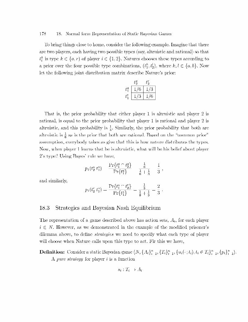
To bring things close to home, consider the following example. Imagine that there
are two players, each having two possible types (say, altruistic and rational) so that
tkiis type k ∈ {a, r) of player i ∈ {1, 2}. Natures chooses these types according to
a prior over the four possible type combinations, (tk1, tl
2), where k, l ∈ {a, b}. Now
let the following joint distribution matrix describe Nature’s prior:
ta2
tr2
ta1
1/6 1/3
tr1
1/3 1/6
That is, the prior probability that either player 1 is altruistic and player 2 is
rational, is equal to the prior probability that player 1 is rational and player 2 is
altruistic, and this probability is 1
3. Similarly, the prior probability that both are
altruistic is 1
6as is the prior that both are rational. Based on the “common prior”
assumption, everybody takes as give that this is how nature distributes the types.
Now, when player 1 learns that he is altruistic, what will be his belief about player
2’s type? Using Bayes’ rule we have,
p1(ta
2|ta1) =
Pr{ta1∩ ta
2}
Pr{ta1}
=1
6
1
6+ 1
3
=1
3,
and similarly,
p1(tr
2|ta1) =
Pr{ta1∩ tr
2}
Pr{ta1}
=1
3
1
6+ 1
3
=2
3.
18.3 Strategies and Bayesian Nash Equilibrium
The representation of a game described above has action sets, Ai, for each player
i ∈ N . However, as we demonstrated in the example of the modified prisoner’s
dilemma above, to define strategies we need to specify what each type of player
will choose when Nature calls upon this type to act. Fir this we have,
Definition: Consider a static Bayesian game 〈N, {Ai}ni=1,{Ti}ni=1, {ui(· ; ti), ti ∈ Ti}ni=1,{pi}n
i=1〉.
A pure strategy for player i is a function
si : Ti → Ai

18.3 Strategies and Bayesian Nash Equilibrium 179
that specifies a pure action si(ti), which is what agent i will choose to do
when his type is ti. Similarly, a mixed strategy is a probability distribution
over a player’s pure strategies.
This is a convenient way to specify strategies. It is as if players choose their
type-contingent strategy before they learn their types, and then play according to
their strategy. This is useful because it allows us to talk about the beliefs of players
over strategies of their opponents, when their opponents can be of different types.
As you can now see, the modified prisoner’s dilemma we used to demonstrate the
central ideas is just a special case of this more general Bayesian game.
To see how the setup we developed gives players the ability to form beliefs
over their opponents’s behavior, and then use these beliefs to calculate their own
expected utility from their actions, consider the example above with two players
and two types, Ti = {tai, tr
i}, and imagine that each player had two pure actions
as in the prisoner’s dilemma, Ai = {M,F}. Now consider the case where player 1
believes that player 2 is using the following strategy
s2(t2) =
{M if t2 = ta
2
F if t2 = tr2
If player 1 is of type ta1, then from his own perspective, his expected utility from
playing M will be,
Eu1 (M,s2 (·) ; ta
1) = p1(t
a
2|ta1) · u1(M,s2(t
a
2); ta
1) + p1(t
r
2|ta1) · u1(M,s2(t
r
2); ta
1)
= p1(ta
2|ta1) · u1(M,M ; ta
1) + p1(t
r
2|ta1) · u1(M,F ; ta
1)
• [EXPAND: a pure strategy + nature’s choices make player i face a mixed
strategy]
• [EXPAND: like in extensive form games, we specify i’s strategy for all infor-
mation sets, even those that are not reached by Nature. the reason is that
to allow player j to form beiefs over i’s behavior, player j needs to combine
the beliefs from his posterior over i’s types, with his beliefs over what each
type ti of player i will do.]
180 18. Normal form Representation of Static Bayesian Games
Once we defined the Bayesian game and the strategies for each player, we can
easily define our newest solution concept, which just builds on the familiar Nash
equilibrium as applied to the Bayesian game we just defined. Namely,
Definition: In the static Bayesian game 〈N, {Ai}ni=1, {Ti}ni=1, {ui(· ; ti), ti ∈ Ti}ni=1, {pi}n
i=1〉 , a
strategy profile s∗ = (s∗1(·), s∗
2(·), ..., s∗
n(·)) is a pure strategy Bayesian Nash
Equilibrium if for every player i, and for each of player i’s types, s∗i(·) solves:
1
∑
t−i∈T−i
pi(t−i|ti)·ui(s∗
i(ti)
︸ ︷︷ ︸
action
for i
, s∗−i
(t−i)
︸ ︷︷ ︸
n−1 action foropponents
; ti) ≥∑
t−i∈T−i
pi(t−i|ti)·ui(ai, s∗
−i(t−i); ti) for all ai ∈ Ai .
(18.1)
That is, regardless of the type realization, no player wants to change his
strategy s∗i(·).
Once we take a static game of incomplete information and transform it to a
Bayesian game as described above, then the “Bayesian” part is in the fact that
for each player’s type realization, we compute his beliefs about the actions of his
opponents using Bayes’ rule. Payoffs from strategy profiles are the expected utility
that is derived from the strategies played by other players, and the mixing that
occurs due to the randomization of nature that each player faces through his beliefs
pi(t−i|ti).
Remark 9 In the definition of Bayesian Nash equilibrium, we can write the con-
dition (18.1) of playing a best response more generally as follows,
Et−i
[ui(s∗
i(ti), s
∗
−i(t−i); ti)|ti] ≥ Et
−i[ui(ai, s
∗
−i(t−i); ti)|ti] for all ai ∈ Ai.
Notice that here we have taken the expectations of player i over the realizations
of types t−i when player i knows his own type (hence, the expectation, Et
−i[·|ti], is
conditional on ti). Once we write it down this way, it is more general in the sense
that it can apply to a continuum of types for each player. That is, it may be the case
1Note that on the right-hand-side of the inequality, we can replace ai with s′
i(ti)∀s
′
i∈ S′
i. But it suffices to
consider any deviation from s∗i(·) to an action, ai, instead of the more complex notion of a type dependent strategy,
s′i(·).

18.3 Strategies and Bayesian Nash Equilibrium 181
that each player has an infinite number of possible types drawn from an interval
Ti = [ti, ti], with cumulative distribution Fi(ti) and density function fi(ti) = F ′
i(ti).
In this case the expected utility of player i will be written as an integral (more
precisely, n − 1 integrals) which form the expectations over the realizations of the
other players’ types, and accordingly, their actions derived from their strategies.
182 18. Normal form Representation of Static Bayesian Games
This is page 1
Printer: Opaq
19
Applications of Bayesian Nash Equilibria
19.1 A Game of Aggression
It is not uncommon for two rivals in some form of conflict to face a decision
of whether to be aggressive or to cave in and expose weakness. Be it firms in
the marketplace, politicians in government, countries at war, or even kids on the
playground, the optimal behavior will depend on some combination of each player’s
tendency to being aggressive, and on his belief about his opponent’s tendency to
be aggressive.
To illustrate this idea, consider a simple game of aggression that is not foreign
to many teenagers: the game of chicken. The 1955 film, Rebel Without a Cause
features James Dean as a juvenile delinquent, an introduced one variant of the
game of chicken to the silver screen. In this movie, two teenagers simultaneously
drive their cars off a cliff. The first one to jump out is chicken, and loses the contest.
(In the movie, one dies, and in real life, James Dean died in a hotrodding accident
just before the film was released.) Many other films featured variations on chicken,
a well known example being the 1978 film Grease staring John Travolta and Olivia
Newton-John. the following example is a variant of this game.
Two teenagers, named 1 and 2, have borrowed their parents’ cars, and decided
to play the game of “chicken” as follows: They both drive towards each other on
184 19. Applications of Bayesian Nash Equilibria
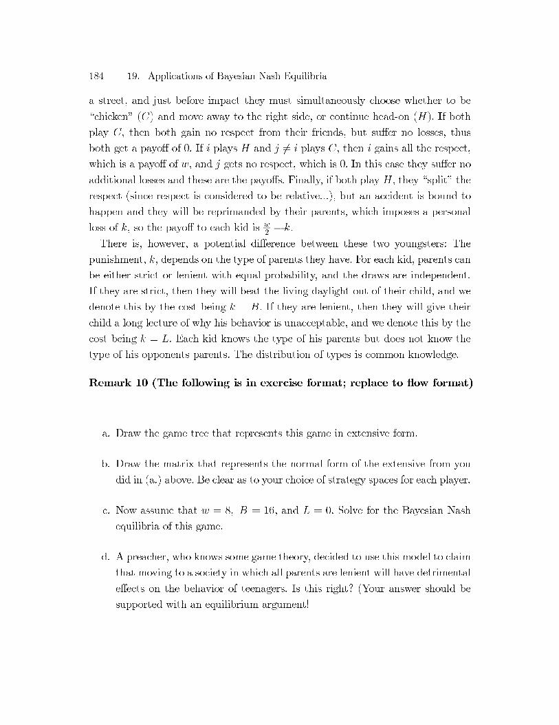
a street, and just before impact they must simultaneously choose whether to be
“chicken” (C) and move away to the right side, or continue head-on (H). If both
play C, then both gain no respect from their friends, but suffer no losses, thus
both get a payoff of 0. If i plays H and j �= i plays C, then i gains all the respect,
which is a payoff of w, and j gets no respect, which is 0. In this case they suffer no
additional losses and these are the payoffs. Finally, if both play H, they “split” the
respect (since respect is considered to be relative...), but an accident is bound to
happen and they will be reprimanded by their parents, which imposes a personal
loss of k, so the payoff to each kid is w
2− k.
There is, however, a potential difference between these two youngsters: The
punishment, k, depends on the type of parents they have. For each kid, parents can
be either strict or lenient with equal probability, and the draws are independent.
If they are strict, then they will beat the living daylight out of their child, and we
denote this by the cost being k = B. If they are lenient, then they will give their
child a long lecture of why his behavior is unacceptable, and we denote this by the
cost being k = L. Each kid knows the type of his parents but does not know the
type of his opponents parents. The distribution of types is common knowledge.
Remark 10 (The following is in exercise format; replace to flow format)
a. Draw the game tree that represents this game in extensive form.
b. Draw the matrix that represents the normal form of the extensive from you
did in (a.) above. Be clear as to your choice of strategy spaces for each player.
c. Now assume that w = 8, B = 16, and L = 0. Solve for the Bayesian Nash
equilibria of this game.
d. A preacher, who knows some game theory, decided to use this model to claim
that moving to a society in which all parents are lenient will have detrimental
effects on the behavior of teenagers. Is this right? (Your answer should be
supported with an equilibrium argument!
19.1 A Game of Aggression 185
FIGURE 19.1.
FIGURE 19.2.
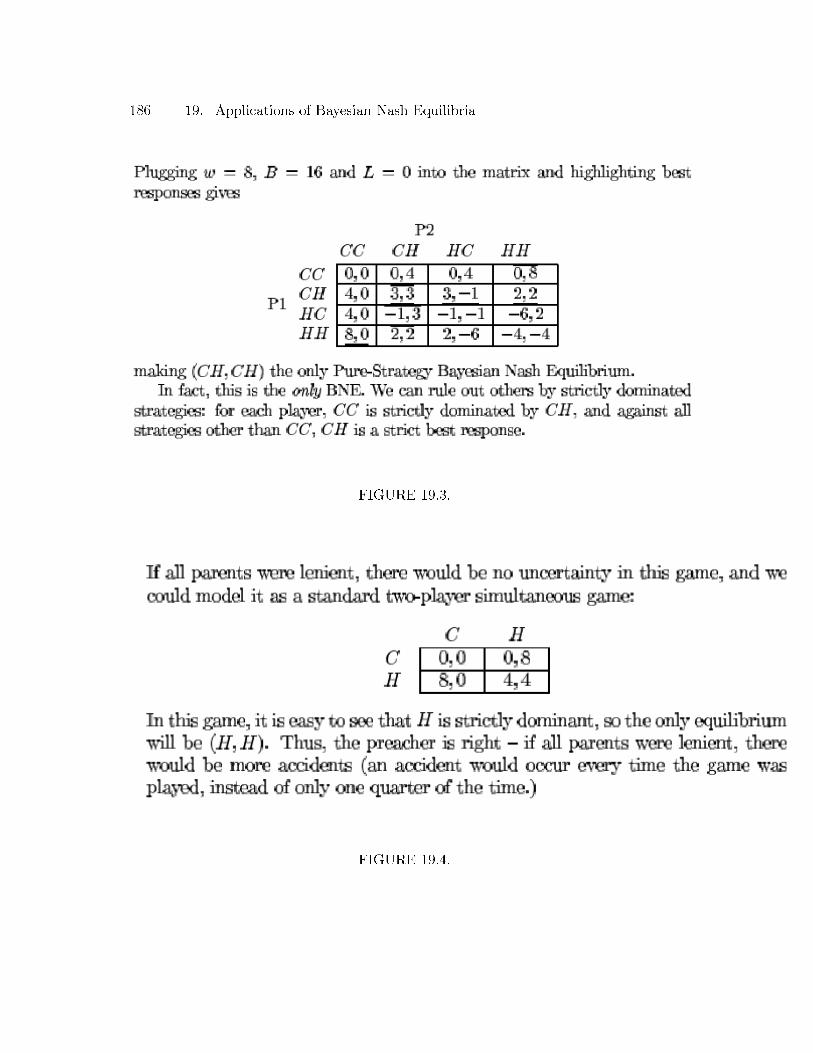
186 19. Applications of Bayesian Nash Equilibria
FIGURE 19.3.
FIGURE 19.4.

19.2 Auctions and Competitive Bidding 187
19.2 Auctions and Competitive Bidding
The use of auctions to sell goods has become as common as apple-pie and french-
fries, thanks to the internet auction house eBayR©
that has invaded many house-
holds across the globe. Previously, a common vision of auctions were the sale of a
Picasso or Renoir in one of the prestigious auction houses of Sotheby’s, that was
created in 1744, and Christie’s, that was created in 1766. It seems that the use of
auctions dates back much further. (For a history of auctions see Ralph Cassidy,
Jr. Auctions and Auctioneering, University of California Press, 1967).
The use of game theory to analyze both behavior in auctions, and the design
of auctions themselves, was introduced by William Vickrey (1961), another Nobel
laureate, and was followed by a large literature that is still expanding. The “big
push” of game theoretical research on auctions happened after the successful use
of game theory to advise both the US government, and the bidding firms, when the
Federal Communications Commission decided to auction off the airwaves for use by
telecommunication companies. This was considered so successful, that a reference
to the work of many game theorists appears in an article in The Economist titled
“Revenge of the Nerds," (The Economist, July 23, 1994, p. 70).
As we will see, auctions have many desirable properties, and these made them
a favorite choice by the US Federal Acquisition Rules as the preferred (by law)
form of procurement in the public sector. They are usually very transparent, they
have well defined rules, they usually allocate the auctioned good to the party who
values it the most, and they are not too easy to manipulate (if well designed).
Generally speaking, there are two common types of auctions. The first type, as we
will refer to it, is the open auction in which the bidders observe some dynamic price
process that evolves until a well defined winner emerges. There are two common
forms of the open auction:
• The “English Auction”: This is the classic auction we will see in a movie
(e.g., The Red violin), where the bidders are all in a room (or nowadays
sitting by a terminal), and the price of the good goes up as long as someone
is willing to bid it up higher. Once the last increase is no longer challenged,
the last bidder to increase the price wins the auction and pays that price.

188 19. Applications of Bayesian Nash Equilibria
(The price may start at some minimum threshold, which would be the seller’s
“reservation” price.)
• The “Dutch Auction”: In many ways this less common auction is the
inverse of the English auction. As with the English auction, the bidders
observe the price change before them, but instead of starting low and rising
by pressure from the bidders, the price starts at a prohibitively high value,
and the auctioneer drops the price gradually. Once a bidder shouts “buy”,
the auction ends and the bidder gets the good at the last price. This auction
was and still is popular in the flower markets of the Netherlands, hence the
name of the auction.
The second common type of auctions is the sealed-bid auction, where partici-
pants write down their bids and submit them without knowing the bids of their
opponents. The bids are collected, and the highest bidder wins and pays a price
that depends on the auction rules. As with open auctions, there are two common
forms of sealed-bid auctions that prevail:
• The “First-Price Sealed-Bid Auction”: This very common auction form
has each bidder write down his bid, or willingness to pay in an envelope, and
the envelopes are opened simultaneously. The highest bidder wins, and then
pays a price equal to his own bid.
• The “Second-Price Sealed-Bid Auction”: As with the First-Price Sealed-
Bid Auction, each bidder writes down his bid in an envelope, and the en-
velopes are opened simultaneously. The difference is that although highest
bidder wins here too, he then pays a price equal to the second highest bid,
or the highest losing bid.
We will start by analyzing the second-price sealed-bid auction because it is the
one that lends itself most easily to formal analysis. As we will see, it has a very
tight relationship with the English auction.
19.2 Auctions and Competitive Bidding 189
19.2.1 Second-Price Sealed Bid Auctions: Independent Private Values
We describe our auction setting as a game with N = {1, 2, ..., n} being the set of
players, and these represent the bidders. We refrain from considering the seller as
a player, since once the auction rules are given by him, he plays no role in bidding
behavior and the outcomes that follow.
We assume that every player has an independent private value of obtaining the
good. For example, you and I can both bid on a Beanie-Baby animal on eBayR©,
and each of us has a value for obtaining the fluffy little critter. However, our values
may be one of many, and we each may not know the value of the other, hence their
private nature. Furthermore, if we assume away the possibility that we are buying
it for resale value and instead only want it for personal use, there is no reason for
my value to depend on yours and vice versa, hence the independence.
To capture this idea we introduce the notion of types. In particular, assume that
the value for player i of obtaining the good is vi ≥ 0, and this value can be one of
many values given by vi ∈ [vi, vi]. We further assume that the actual value of vi is
drawn from this interval [vi, vi] according to the cumulative distribution function
Fi (·) , where Fi (v′) = Pr{vi � v′}. The utility of a player who does not get the
good is normalized to zero, and the utility of a player who gets the good and pays
a price p ≥ 0 is ui = vi − p.
Since we are using the methodology of Bayesian games, we will assume that
every player knows the distribution of all types of the other players, and uses the
n − 1 cumulative distribution functions Fj (·) , j �= i, to form beliefs about the
types t−i of the other players.
The rules of the game are as follows. First, players learn their private valuations,
but only know the probabilistic information about their opponents. Second, each
player submits a bid bi ≥ 0, which is the action each player can choose. Finally,
the bids are collected, the highest bidder wins, and he pays a price equal to the

190 19. Applications of Bayesian Nash Equilibria
second highest bid. Thus, we can write the payoff function of each player i as,1
ui(bi, b−i; vi) =
{vi − b
∗
j if bi > bj∀j �= i and b∗j ≡ max{bj}, j �= i
0 if bi � bj , for some j �= i
Given that a player’s action is his bid, we know from the development of Bayesian
games that a player’s strategy must be a mapping that assigns a bid to each of
the player’s types, in this case, private valuations. Thus, a strategy for player i is
a function si : [vi, vi]→ �+ that assigns a non-negative bid to each of his possible
valuations.
Now, we can write down the utility of player i with valuation vi, as a function
of his own bid bi and the strategies used by the other players sj(·), j �= i. First,
it is worth writing down a short-hand expression for player i’s expected utility as
follows:
Et−i
[ui(bi, s−i(v−i); vi)|vi] = Pr{i wins and pays p} · (vi − p) + Pr{i looses} · 0
In more specific terms, taking into account the rules of the second-price sealed bid
auction, the probability that player i wins is equal to the probability that all the
other bids are below bi, and in this event the price player i pays is the second
highest bid. What is the probability that all the other bids are below bi? This is a
relatively easy expression due to the independence assumption on the distribution
of valuations.
First notice that if player j �= i is using the bid function sj(vj), then the prob-
ability that i’s bid is higher than j’s bid is clearly equal to the probability that j
is a type (has a value) that bids less than bi, but without knowing exactly what
j’s strategy is we cannot write this probability down. So, let’s make a reasonable
assumption on the bidding behavior of player:
Assumption: The higher a player’s valuation, the higher is his bid: if v′
j > v′′
j
then sj(v′
j) > sj(v′′
j ).
1Notice that we resolve the possibility of two players tied with the highest bid by assuming that then neither
gets the good and both pay nothing. This can be easily changed to have them randomly be the winner, and pay
the second highest price, which would be equal to their own bid (since the two tied as the highest bid). This would
add negligible complications, some that will be mentioned later.
19.2 Auctions and Competitive Bidding 191
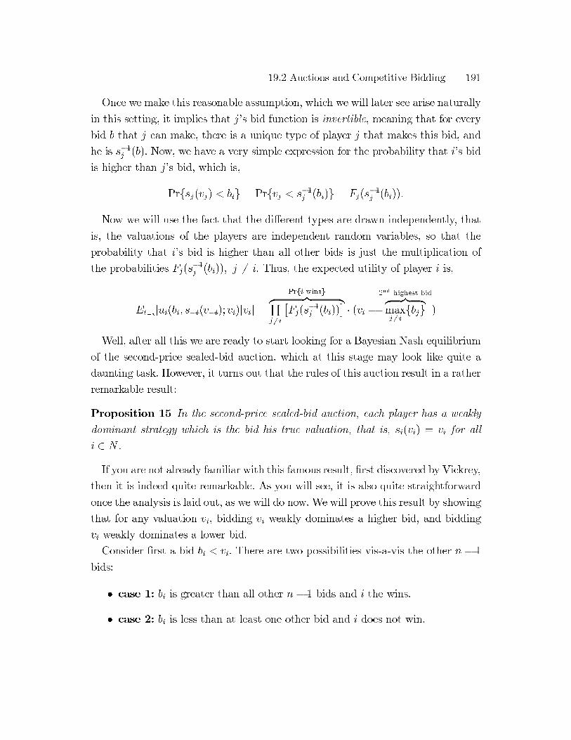
Once we make this reasonable assumption, which we will later see arise naturally
in this setting, it implies that j’s bid function is invertible, meaning that for every
bid b that j can make, there is a unique type of player j that makes this bid, and
he is s−1j (b). Now, we have a very simple expression for the probability that i’s bid
is higher than j’s bid, which is,
Pr{sj(vj) < bi} = Pr{vj < s−1j (bi)} = Fj(s−1
j (bi)).
Now we will use the fact that the different types are drawn independently, that
is, the valuations of the players are independent random variables, so that the
probability that i’s bid is higher than all other bids is just the multiplication of
the probabilities Fj(s−1
j (bi)), j �= i. Thus, the expected utility of player i is,
Et−i[ui(bi, s−i(v−i);vi)|vi] =
Pr{i wins}︷ ︸︸ ︷∏j �=i
[Fj(s
−1
j (bi))]
· (vi −
2nd highest bid︷ ︸︸ ︷
max
j �=i{bj} )
Well, after all this we are ready to start looking for a Bayesian Nash equilibrium
of the second-price sealed-bid auction, which at this stage may look like quite a
daunting task. However, it turns out that the rules of this auction result in a rather
remarkable result:
Proposition 15 In the second-price sealed-bid auction, each player has a weakly
dominant strategy which is the bid his true valuation, that is, si(vi) = vi for all
i ∈ N .
If you are not already familiar with this famous result, first discovered by Vickrey,
then it is indeed quite remarkable. As you will see, it is also quite straightforward
once the analysis is laid out, as we will do now. We will prove this result by showing
that for any valuation vi, bidding vi weakly dominates a higher bid, and bidding
vi weakly dominates a lower bid.
Consider first a bid bi < vi. There are two possibilities vis-a-vis the other n − 1
bids:
• case 1: bi is greater than all other n − 1 bids and i the wins.
• case 2: bi is less than at least one other bid and i does not win.

192 19. Applications of Bayesian Nash Equilibria
FIGURE 19.5.
In the case 1, bidder i wins and pays maxj �=i{bj}. If instead of bidding bi he
would have bid vi > bi, then he would still win and pay the same price, making
him indifferent between the two options. So, in case 1 bidding his valuation weakly
dominates bidding bi.
In case 2, there are two possibilities. The first is that the highest bid is above
player i’s valuation. Once again, if instead of bidding bi he would have bid vi > bi,
then he would still lose the auction since maxj �=i{bj} > vi, making him indifferent
between the two options. So, in this first possibility of case 2, bidding his valuation
weakly dominates bidding bi.
Now we come to the last possible realization, a second possibility of case two
in which the second highest bid is above i’s bid, but below his valuation: vi >
maxj �=i{bj} > bi. By bidding bi, i loses the auction and gets a utility of zero. If,
instead, he would have bid vi, he would have won the auction and received a utility
of
ui = vi −max
j �=i
{bj} > 0,
making this a profitable deviation. Thus, we conclude that bidding vi weakly domi-
nates any lower bid because it is never worse, and sometimes better, as summarized
in figure ??.

19.2 Auctions and Competitive Bidding 193
Exercise 5 Convince yourself using a similar argument that a bid bi > vi will
also be weakly dominated by bidding vi. (Hint: in this case you would either be as
well off, or prevent a loss.)
This fact that every player has a weakly dominant strategy, si(vi) = vi,
implies the following important corollary:
Corollary 16 In a second-price sealed-bid auction with independent private val-
ues, each player bidding his valuation is a Bayesian Nash Equilibrium in weakly
dominant strategies.
This result is remarkable not only because of its simple recommendation value,
that players bid their valuations truthfully in a second-price sealed-bid auction,
but also implies three other attractive features of this auction format:
• — Feature 1: In a private values setting, bidders in a second-price sealed-
bid auction do not care about the probability distribution over their
opponents’ types, and therefore the assumption of common knowledge
of the distribution of types can be discarded when such auctions are
analyzed. In particular, it means that we can apply this result even when
we think that players have no idea about their opponents’ valuations.
— Feature 2: in a second-price sealed-bid auction, even if types are cor-
related, but values are private, then it is a weakly dominant strategy to
bid truthfully. This again means that if we are correct about our private
values assumption, then even if we incorrectly think that values are in-
dependent, the argument that bidding your true valuation is a weakly
dominant strategy is still true.
— Feature 2: in a second-price sealed-bid auction, the outcome is Pareto
Optimal, as the result will be that the person who values the good most
will be the one who gets it.
Thus, we conclude that the second-price sealed-bid auction has many wonderful
characteristics, both resulting in prescription for very simple strategies, and out-
comes that are Pareto optimal. As will now briefly see, the second-price sealed-bid
auction is closely related to the very common English auction.
194 19. Applications of Bayesian Nash Equilibria
Remark 11 We can change the game to be more appealing with respect to the
treatment of tied high bids. Assume that if m � n bidders tie with the highest bid,
then they are each equally likely to win, and they pay the second highest bid, which
by definition is equal to their own bid in the case of a tie. Then, the payoff function
of each bidder can be written as
ui(bi, b−i; vi) =
vi − b∗j if bi > bj∀j �= i and b∗j ≡ max{bj}, j �= ivi−bi
#{highest bidders}if bi ≥ bj∀j �= i and bi = bj for some j �= i
0 if bi < bj , for some j �= i
You should be able to convince yourself that the arguments leading to bi = vi being
a weakly dominant strategy are still valid, and this, the analysis above applies.
L14
19.2.2 English Auctions with Independent Private Values
• public sequential bidding: people in a room increase the last bid to a new
one, and everyone observes the price progression.
• The last bidder to increase the current price, without having another bidder
increase it further is the winner, and he pays his bid.
• How would we describe this as a game? There is a problem: without discrete
increments, there is no best response if p < vi (similar to the problem we
had in the Bertrand model, a player may wish to increase the bid, but there
is no optimal increase if bids can be from a continuum).
• Two solutions: either (1) Use discrete action spaces such as dollars and cents.
This is realistic, but we cannot apply elegant techniques such as derivatives
to find optimal behavior, and this makes the analysis very cumbersome; or
(2) change the game without losing the spirit of English auctions, which is
what Milgrom and Weber (1982) did in their “button-model” auction. It
proceeds as follows:
1. As before, there are n players with valuations vi ∈ [vi, vi] drawn accord-
ing to the cumulative distribution function Fi (·), and one auctioneer that
announces the current price, starting at p = 0 and rising continuously.

19.2 Auctions and Competitive Bidding 195
2. Each player has a button that is pressed at the beginning of the game when
the starting price is p = 0. If the button of player i is continuously pressed
and the current price is p > 0, this means that player i is willing to pay p if
everyone else would drop out of the auction now.
3. Once a player releases his button, he is dropped from the auction and cannot
re-enter.
4. The winner is the last person to hold on to his button. The price is the posted
price at which the before-last player let go of his button.
• Once again, as with the second-price sealed bid auction, we can set up the
strategies for each player (which in this case are maps from type, or valuation,
to the price at which a player lets go of his button), and we can then derive
the expected utility functions of very player given his beliefs about the other
players’ strategies and types. However, as with the second-price sealed-bid
auction, we have the following remarkable, though more anticipated result:
Proposition 17 In the button-version English auction, each player has a weakly
dominant strategy which is to keep holding his button pressed as long as p < vi
and to release it one p = vi. This results in a weakly dominant Bayesian Nash
equilibrium, that is outcome-equivalent to the second-price sealed-bid auction.
• This follows precisely because of the following simple observations:
1. if the “current price” is p < vi, then clearly, player i (who is not the
currently highest bidder) should continue holding his button, therefore
causing the price to increase further.
2. if p > vi, player i should have dropped out.
• Thus, the solution is just like in the second-price sealed-bid auction: the
player with the highest valuation wins, and he pays a price equal to the
second highest valuation.
196 19. Applications of Bayesian Nash Equilibria
• Note that on eBayR©, the way the auctions work is very similar to this button
model since eBayR©
uses a “proxy bidding” system that takes your bid, but if
you are the highest bidder then the current price is one increment above the
second highest bidder, in a similar fashion to the button model. Interestingly,
the instructions on eBayR©
suggest that you bid truthfully: “When you place
a Bid, enter the maximum amount you are willing to pay for the item. eBay
will bid on your behalf only if there is a competing bidder and only up to your
maximumamount.” (http://pages.ebay.com/education/buyingtips/index.html#bid)
19.2.3 Dutch and First-Price Sealed-Bid Auction
• Question: Is it a weakly dominant strategy to bid your valuation in a first-
price sealed-bid auction where the highest bidder wins and pays his bid?
• The answer is generally no: By bidding your valuation, Eu = 0 (if you lose
you get 0, and if you win you pay your valuation, thus you are left with 0).
If, however, you bid less than your valuation, then Eu > 0 (there is some
probability that you will win, multiplied by some positive utility of your
value less your bid).
• How do we solve this game? What is the best response of a player?
• Unlike the very appealing result of second-price sealed-bid auctions, the play-
ers do not have a weakly dominant strategy that maps types to bids, and their
best response depends on the belief over other people’s bids/type-dependent
strategies. Thus, the distributional assumptions will matter, and the common
knowledge assumption on a common prior has real bite.
• It turns out that the Dutch and first-price sealed-bid auction are closely
related in the sense that they have the same set of Bayesian Nash equilibrium.
• (Intuition: the bid in the first-price sealed-bid auction (or the acceptance
price in the Dutch auction) is determined by a marginal-cost-marginal benefit
trade-off. By lowering your bid incrementally, you increase your margin when
you win, which is the marginal benefit. At the same time, the probability of
winning becomes lower, which is the marginal cost.
19.2 Auctions and Competitive Bidding 197
• (add an example to complete this section)
19.2.4 Common Values and the Winner’s Curse
The private values scenario was one where each player’s utility depended on the
profile of actions of all players, but only on his own type. This setting is useful in
describing some scenarios like how much different people value a hamburger, or a
bag of chips, but in many cases the utility of one player will depend on the private
information of other players.
Consider, for instance, a house that is on the market — how much would you be
willing to pay for it? The answer will depend on two major components: first, your
own private value of living in that house, and second, what you expect to get for
the house if you choose to sell it at a later date. The valuation of other people will
therefore enter into your willingness to pay for a house, and this will generally be
their own private information. This same argument will apply to a piece of art, a
car, or even a movie — you may value a movie more if you think other people value
it more, so you can later talk to them about it and all agree on how good (or bad)
it was.
We refer to such scenarios as having a common values element. To illustrate
an extreme example of common values, imagine that two identical oil firms are
considering the purchase of a new oil field. It is common knowledge that the amount
of oil is either small, worth 10 million dollars of net profits, medium, worth 20
million dollars of net profits, or large, worth 30 million dollars of net profits. Thus,
the oil field has one of three values, v ∈ {10,20, 30}. Imagine that it is also common
knowledge that these values are distributed so that it is equally likely that the
amount is small or large, and twice as likely that it is medium, so that
Pr{v = 10} = Pr{v = 30} =1
4, and Pr{v = 20} =
1
2.
Now assume that the government, who currently owns the field, will auction it
off in a second-price sealed-bid auction, and that before the auction each firm will
perform a (free) exploration that will provide some signal about the quantity of
oil in the field. Specifically, each player receives a low or high signal, si = {L,H},
which is correlated with the amount of oil as follows:

198 19. Applications of Bayesian Nash Equilibria
• if v = 10, then s1 = s2 = L;
• if v = 30, then s1 = s2 = H;
• if v = 20, then either s1 = L and s2 = H, or s1 = H and s2 = L, each event
occurring with equal probability;
Thus, the probabilities of each pair of signals is given by the following table,
s1\s2 L H
L 1/4 1/4
H 1/4 1/4
and the signal outcomes are not independent — they are correlated with the actual
amount of oil.
We can associate each player’s signal with his type, to the extent that given a
signal, a player can form expectations about the signal of his opponent, and about
the quantity of oil. Namely, if player i observes a low signal L, then he knows that
the probability that his opponent got a low signal is equal to the probability he
received a high signal, which is 1
2. Similarly, Pr{sj = H|si = H} = Pr{sj = L|si =
H} = 1
2.
Given these updated probabilities that each type has, we can calculate the ex-
pected amount of oil in the field conditional on the signal a player has. If player i
observes a low signal, he knows that with probability 1
2the other signal is low, and
v = 10, and with probability 1
2the other signal is high, and v = 20. Therefore,
E[vi|si = L] =1
2· 10 +
1
2· 20 = 15,
and similarly,
E[vi|si = H] =1
2· 20 +
1
2· 30 = 25.
At this stage we have identified the way types map into expectations over the
amount of oil, and therefore, they map into expected utilities from owning the
field. However, it is not true that one player’s type alone determines the value of
obtaining the oil field — there is valuable information in the type of the other player,

19.2 Auctions and Competitive Bidding 199
which as we will now see, makes the previously attractive second-price sealed-bid
auction somewhat less straightforward.
To see this, let’s first consider the following question: is it a Bayesian Nash equi-
librium for both players to submit truthful bids equal to there expected valuation?
Formally, is bi = Evi for i ∈ {1, 2} a Bayesian Nash equilibrium? To check this
let’s assume that player 2 is playing in this truthful fashion, and check whether
bidding truthfully is a best response of player 1. When s1 = H and he bids 25,
then with probability 1
2his opponent also received a high signal and bids 25, in
which case they win with equal probability and pay the second highest bid of 25
(they tied). With probability 1
2player 2 has a low signal and player 1 wins and
pays player 2’s bid of 15. Therefore,his expected utility is
Eui =1
2[1
2· (30− 25)] +
1
2[20− 15] = 3.75
Similarly, when s1 = L and player 1 bids 15, then with probability 1
2his opponent
also bids 15, in which case they win with equal probability and pay the second
highest bid of 15. With probability 1
2player 2 has a high signal and player 1 loses,
giving him a payoff of zero. Therefore, his expected utility is,
Eui =1
2[1
2· (10 − 15)] +
1
2[0] = −1.25
Why is it that when they each bid their valuation, they receive expected negative
payoffs some of the time? This is a result of the common values and the correlated
types. When a player wins the oil field because his opponent’s bid was lower, then
this is “bad news” to the extent that the opponent’s low signal means that the
quantity of oil is lower than the player thinks it is.
This a phenomenon which occurs with common values, and is known as the
“Winner’s Curse”: a player wins when his signal is the most optimistic, which due
to the common value element means that he has over estimated the value of the
good, and is overpaying.
This phenomenon exists in first- and second-price sealed-bid auctions, and has
important economic consequences as to which auctions may perform better in
allocating a common value good efficiently.
(to be completed...)

200 19. Applications of Bayesian Nash Equilibria
19.3 Inefficient Trade and Adverse Selection
One of the main conclusions of competitive market analysis in economics is that
markets allocate goods to the people who value them the most. The simple intuition
behind this conclusion works as follows: If a good is misallocated so that some
people who have it value it less than people who do not, then so called “market
pressures” will cause the price of that good to increase to a level where the current
owners will prefer to sell it, rather than hold on to it, and the people who value
it more will be willing to pay that price. The determination of such a price is not
clearly specified, but various mechanisms such as bargaining, auctions, or market
intermediaries may obtain it.
This powerful argument is based on some assumptions, one of which is that the
value of the good is easily understood by all market participants, or in our termi-
nology, there is perfect information about the value of the good. This is, of course,
an assumption that applies to an ideal world, one that often departs from the re-
ality in which we live. Yet, under this assumption we not only obtain this amazing
result, but we also get what is known as the “Coase Theorem”, named after its
contributor Ronald Coase. It argues that in a world with perfect information and
no market frictions (referred to as “transactions costs”), the allocation of property
rights will not affect economic efficiency. That is, even if for some reason goods
are allocated to the people who do not value them the most, then with perfect
information and well functioning abilities to exchange goods, these goods will end
up in the hands of those who value them the most.
It is therefore important to understand the extent to which these arguments
stand or fall in the face of incomplete information, where some people are more
informed about the value of goods than others. To address this question we will
develop a simple example that follows in the spirit of an important contribution
made by George Akerlof (1970), a contribution that introduced the idea of adverse
selection into economics, and earned its author a Nobel prize.
Imagine a scenario where player 1 owns an orange grove. The yield of fruit
depends on the quality of soil and other local conditions, and assume that through
his experience only player 1 knows the quality of land. Local geological surveys
conclude that the quality of land can be poor, mediocre or good, each with equal
19.3 Inefficient Trade and Adverse Selection 201
probability of 1
3, with monetary-equivalent values for player 1, v1 ∈ {10, 20, 30}.
Thus, we can think of the knowledge of player 1 as his type, T1 = {tL1, tM
1, tH
1},
where each type has a different value for the land so that his utility from owning
the land is v1(own|t1) as described above.
Now imagine that player 2 is a potential soy-bean grower, who is considering the
purchase of this land for his production. Player 2’s family expertise of growing soy-
beans is very profitable, but also depends on the quality of the land. In particular,
for poor, mediocre or good land, player 2’s monetary-equivalent values are v2 ∈
{14, 24, 34}. The problem, however, is that player 2 only knows that the quality id
distributed equally among the three options (the geological survey’s results) but
does not know which of the three it is.
Consider the following game: player 2 makes a take-it-or-leave-it offer to player
1, after which player 1 can accept (A) or reject (R) the offer, and the game ends
with either a transfer of land for the suggested price, or no transfer. A strategy for
player 2 is therefore a single price offer, p, and a strategy for player 1 is a mapping
from his type space T1 to a response, s1 : T1 → {A,R}. What can emerge as an
equilibrium of this game?
The assumptions on payoffs imply that from an efficiency point of view, it is
player 2 who should own the land. Indeed, if the quality of land were common
knowledge then there are many prices for which both player 1 and player 2 would
be happy to trade the property. For example, if the quality is known to be low,
then in a similar way to the one-period bargaining model, the unique subgame
perfect equilibrium would have player 2 offering player 1 a price of 10, and player
1 accepting. Similarly, any price between 10 and 14 would be supported by some
Nash equilibrium.2 We will now see what kind of trade could occur in equilibrium,
when there is asymmetric information as described.
Let’s consider the value that player 2 places on the land. He knows that with
equal probability it is worth one of the values v2 ∈ {14, 24, 34}, so on average it is
worth 24. He also knows that on average it is worth 20 to player 1. It would seem
2Namely, for any p∗∈ [10, 14], a strategy for player 1 accepting any offer p ≥ p
∗ and a strategy for player 2 of
offering p∗ would be a Nash equilibrium when the quality is low.

202 19. Applications of Bayesian Nash Equilibria
that the natural equilibrium candidate would be to offer the lowest price at which
player 2 thinks that player 1 will accept, and such an offer would be p = 20.
But what would then be player 1’s response? Recall that player 1 knows the
quality of land, in which case player 1 would accept the offer only if his type is tL1
or tM
1, meaning that player 2 would get a parcel of land that is of low or mediocre
with equal probability, and get an expected value of 19, and he would make a loss!3
Notice that for any offer p ∈ [20, 30) player 1 would accept the offer only if his
type is tL1or tM
1, and player 2’s value is still 19 on expectation, making such a
trade impossible in equilibrium. Thus, if player 2 is to take into account the best
response of player 1, he knows that he will get all types of player 1 to agree to sell
only if player 2 offers 30, but in this case he would only get a value of 24, which is
not profitable. Therefore, we conclude that no trade can occur at a price greater
than 20.
This implies that if trade is to occur, it will occur at a price less than 20, which
in turn implies that player 1 will agree to such a trade only if his type is tL1. Taking
this into account, player 2 should offer a price p = 10, commensurate with player
1 trading if his type is indeed tL1. This logic yields the following result:
Proposition 18 Trade can occur in Bayesian Nash Equilibrium only if it involves
the lowest type of player 1 trading. Furthermore, any price p∗
∈ [10, 14] can be
supported as a Bayesian Nash equilibrium.
The reason that only the lowest type can trade in equilibrium follows from our
analysis above. To see that any price p∗
∈ [10, 14] can be supported as a Bayesian
Nash equilibrium consider the following strategies: player 2 offers a price p∗, and
the strategy for player 1 is:
s1(t1) =
A if and only if p ≥ p∗ and R otherwise when t1 = tL
1
A if and only if p ≥ 20 and R otherwise when t1 = tM1
A if and only if p ≥ 30 and R otherwise when t1 = tH1
In this case, the two strategies are mutual best responses, and therefore they con-
stitute a Bayesian Nash equilibrium.
3This follows from Bayes’ rule: if only tL
1or t
M
1types ell, then conditional on a sale, each of these types occurs
with probability 1
2.
19.4 Mixed Strategies Revisited: Harsanyi’s Interpretation♠♠ 203
The conclusion of this result is that trade will occur only if the quality of land is
the lowest. The reason this happens is because of what is called “adverse selection”.
When the buyer is willing to pay a price equal to his average value, then the type
of seller who is willing to sell at this price is below average, because the best
types choose not to participate at an average price, hence the adverse selection of
lower than average sellers. In the example, this unravelling causes traded quality
to drop to its lowest level, preventing the market from implementing efficient trade
outcomes.
It is also worth mentioning that this scenario falls into the category of common
values, since the type of player 1 affects the payoff of player 2. It is precisely this
that causes the adverse effects of equilibrium when there is this kind of asymmetric
information.
(add the fact that “cheap talk” would not help here, and allude to the
possibility of costly signalling)
19.4 Mixed Strategies Revisited: Harsanyi’s Interpretation♠♠
Recall the static game of matching pennies,
H T
H
T
1,−1 −1, 1
−1,1 1,−1
and recall that the unique mixed strategy equilibrium has each player playing
heads with probability 1
2. One reason this solution may be somewhat unappealing
is that players are indifferent between H and T , yet they are prescribed to ran-
domize between these strategies in a unique and particular way for this to be a
Nash equilibrium. Does it make sense to ask for this requirement when a player is
indifferent?
This question has caused some discomfort with the notion of mixed strategy
equilibria. However, John Harsanyi (1973) offered a twist on the basic model of
behavior to resolve this problem and alleviate, to some extent, the indifference
problem. His idea works as follows. Imagine that each player may have some slight
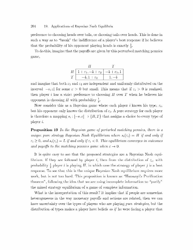
204 19. Applications of Bayesian Nash Equilibria
preference to choosing heads over tails, or choosing tails over heads. This is done in
such a way as to “break” the indifference of a player’s best response if he believes
that the probability of his opponent playing heads is exactly 1
2.
To do this, imagine that the payoffs are given by this perturbedmatching pennies
game,
H T
H 1+ ε1,−1 + ε2 −1 + ε1, 1
T −1, 1 + ε2 1,−1
and imagine that both ε1 and ε2 are independent and uniformly distributed on the
interval [−ε, ε] for some ε > 0 but small. This means that if εi > 0 is realized,
then player i has a strict preference to choosing H over T when he believes his
opponent is choosing H with probability 1
2.
Now consider this as a Bayesian game where each player i knows his type, εi,
but his opponent only knows the distribution of εi. A pure strategy for each player
is therefore a mapping si : [−ε, ε] → {H,T} that assigns a choice to every type of
player i.
Proposition 19 In the Bayesian game of perturbed matching pennies, there is a
unique pure strategy Bayesian Nash Equilibrium where si(εi) = H if and only if
εi ≥ 0, and si(εi) = L if and only if εi < 0. This equilibrium converges in outcomes
and payoffs to the matching pennies game when ε→ 0.
It is quite easy to see that the proposed strategies are a Bayesian Nash equi-
librium. If they are followed by player i, then from the distribution of ει, with
probability 1
2player i is playing H, in which case the strategy of player j is a best
response. To see that this is the unique Bayesian Nash equilibrium requires more
work, but is not too hard. This proposition is known as “Harsanyi’s Purification
theorem”, following the idea that we are using incomplete information to “purify”
the mixed strategy equilibrium of a game of complete information.
What is the interpretation of this result? It implies that if people are somewhat
heterogeneous in the way monetary payoffs and actions are related, then we can
have uncertainty over the types of players who are playing pure strategies, but the
distribution of types makes a player have beliefs as if he were facing a player that
19.4 Mixed Strategies Revisited: Harsanyi’s Interpretation♠♠ 205
is playing a mixed strategy. Harsanyi argues that using mixed strategy equilibria
in simple games of complete information can be thought of as a solution to the
more complex games of incomplete information, in which players do not randomize
but rather have strict best responses.
![Information-Bearing Noncoherently Modulated Pilots for ...people.ece.umn.edu/users/nihar/papers/info_noncoherent.pdf · min f N; b T= 2 cg [29], the optimal input has indeed a USTM](https://static.fdocuments.us/doc/165x107/5f53ed6fda34c965815017ab/information-bearing-noncoherently-modulated-pilots-for-min-f-n-b-t-2-cg-29.jpg)