22 November 2005. Eric Rasmusen, Erasmuse@indiana.edu. Http://www.rasmusen.org.

Part II Asymmetric Information

193

7 Moral Hazard: Hidden Actions

7.1 Categories of Asymmetric Information Models

It used to be that the economist’s first response to peculiar behavior which seemed tocontradict basic price theory was “It must be some kind of price discrimination.” Today,we have a new answer: “It must be some kind of asymmetric information.” In a game ofasymmetric information, player Smith knows something that player Jones does not. Thiscovers a broad range of models (including price discrimination itself), so it is notsurprising that so many situations come under its rubric. We will look at them in fivechapters.

Moral hazard with hidden actions (Chapters 7 and 8)Smith and Jones begin with symmetric information and agree to a contract, but then

Smith takes an action unobserved by Jones. Information is complete.

Adverse selection (Chapter 9)Nature begins the game by choosing Smith’s type, unobserved by Jones. Smith and

Jones then agree to a contract. Information is incomplete.

Mechanism design in adverse selection and post- contractual hidden knowledge )(Chapter 10)

Jones is designing a contract for Smith designed to elicit Smith’s private information.This may happen under adverse selection— in which case Smith knows the informationprior to contracting— or post-contractual hidden knowledge (also called moral hazardwith hidden information)—in which case Smith will learn it after contracting.

Signalling and Screening (Chapter 11)Nature begins the game by choosing Smith’s type, unobserved by Jones. To

demonstrate his type, Smith takes actions that Jones can observe. If Smith takes theaction before they agree to a contract, he is signalling. If he takes it afterwards, he isbeing screened. Information is incomplete.

The important distinctions to keep in mind are whether or not the players agree to acontract before or after information becomes asymmetric, and whether their own actionsare common knowledge. Not all the terms I used above are firmly established. Inparticular, some people would say that information becomes incomplete in a model ofpost-contractual hidden knowledge, even though it is complete at the start of the game.That statement runs contrary to the definition of complete information in Chapter 2,however.

We will make heavy use of the principal-agent model. Usually this term is applied tomoral hazard models, since the problems studied in the law of agency usually involve anemployee who disobeys orders by choosing the wrong actions, but the paradigm is usefulin all four contexts listed above. The two players are the principal and the agent, who areusually representative individuals. The principal hires an agent to perform a task, andthe agent acquires an informational advantage about his type, his actions, or the outsideworld at some point in the game. It is usually assumed that the players can make a

194

binding contract at some point in the game, which is to say that the principal cancommit to paying the agent an agreed sum if he observes a certain outcome. In thebackground of such models are courts, which will punish any player who breaks a contractin a way that can be proven with public information.

The principal (or uninformed player) is the player who has the coarser informationpartition.

The agent (or informed player) is the player who has the finer information partition.

Figure 1: Categories of Asymmetric Information Models

Figure 1 shows the game trees for five principal-agent models. In each model, theprincipal (P) offers the agent (A) a contract, which he accepts or rejects. In some, Nature(N) makes a move, or the agent chooses an effort level, message, or signal. The moralhazard models are games of complete information with uncertainty. The principal offers acontract, and after the agent accepts, Nature adds noise to the task being performed. Inmoral hazard with hidden actions, Figure 1(a), the agent moves before Nature and inmoral hazard with hidden knowledge, Figure 1(b), the agent moves after Nature andconveys a “message” to the principal about Nature’s move.

Adverse selection models have incomplete information, so Nature moves first and

195

picks the type of the agent, generally on the basis of his ability to perform the task. Inthe simplest model, Figure 1(c), the agent simply accepts or rejects the contract. If theagent can send a “signal” to the principal, as in Figures 1(d) and 1(e), the model issignalling if he sends the signal before the principal offers a contract, and screeningotherwise. A “signal” is different from a “message” because it is not a costless statement,but a costly action. Some adverse selection models include uncertainty and some do not.

A problem we will consider in detail arises when an employer (the principal) hires aworker (the agent). If the employer knows the worker’s ability but not his effort level, theproblem is moral hazard with hidden actions. If neither player knows the worker’s abilityat first, but the worker discovers it once he starts working, the problem is moral hazardwith hidden knowledge. If the worker knows his ability from the start, but the employerdoes not, the problem is adverse selection. If, in addition to the worker knowing hisability from the start he can acquire credentials before he makes a contract with theemployer, the problem is signalling. If the worker acquires his credentials in response to awage offer made by the employer, the problem is screening.

The five categories are not uniformly recognized, and in particular, some would arguethat what I have called “moral hazard with hidden knowledge” and “screening” areessentially the same as adverse selection. Myerson (1991, p. 263), for example, suggestscalling the problem of players taking the wrong action “moral hazard” and the problem ofmisreporting information “adverse selection.” Or, the two problems can be called “hiddenactions” versus “hidden knowledge”. (The separation of asymmetric information intohidden actions and hidden knowledge is suggested in Arrow [1985] and commented on inHart & Holmstrom [1987]). Many economists do not realize that screening and signallingare different and use the terms interchangeably. “Signal” is such a useful word that it isoften used simply to indicate any variable conveying information. Most people have notthought very hard about any of the definitions, but the importance of the distinctions willbecome clear as we explore the properties of the models. For readers whose minds aremore synthetic than analytic, Table 1 may be as helpful as anything in clarifying thecategories.

Table 1: Applications of the Principal-Agent Model

196

Principal Agent Effort or type and signal

Moral hazard with Insurance company Policyholder Care to avoid thefthidden actions Insurance company Policyholder Drinking and smoking

Plantation owner Sharecropper Farming effortBondholders Stockholders Riskiness of corporate projectsTenant Landlord Upkeep of the buildingLandlord Tenant Upkeep of the buildingSociety Criminal Number of robberies

Moral hazard with Shareholders Company president Investment decisionhidden knowledge FDIC Bank Safety of loans

Adverse selection Insurance company Policyholder Infection with HIV virusEmployer Worker Skill

Signalling and Employer Worker Skill and educationscreening Buyer Seller Durability and warranty

Investor Stock issuer Stock value and percentage retained

Section 7.2 discusses the roles of uncertainty and asymmetric information in aprincipal-agent model of moral hazard with hidden actions, called the Production Game,and Section 7.3 shows how various constraints are satisfied in equilibrium. Section 7.4collects several unusual contracts produced under moral hazard and discusses theproperties of optimal contracts using the example of the Broadway Game.

7.2 A Principal-Agent Model: The Production Game

In the archetypal principal-agent model, the principal is a manager and the agent aworker. In this section we will devise a series of these games, the last of which will be thestandard principal-agent model.

Denote the monetary value of output by q(e), which is increasing in effort, e. Theagent’s utility function U(e, w) is decreasing in effort and increasing in the wage, w, whilethe principal’s utility V (q − w) is increasing in the difference between output and thewage.

The Production Game

Players

197

The principal and the agent.

The order of play1 The principal offers the agent a wage w.2 The agent decides whether to accept or reject the contract.3 If the agent accepts, he exerts effort e.4 Output equals q(e), where q′ > 0.

PayoffsIf the agent rejects the contract, then πagent = U and πprincipal = 0.If the agent accepts the contract, then πagent = U(e, w) and πprincipal = V (q − w).

An assumption common to most principal-agent models is that either the principalor the agent is one of many perfect competitors. In the background, either (a) otherprincipals compete to employ the agent, so the principal’s equilibrium profit equals zero;or (b) many agents compete to work for the principal, so the agent’s equilibrium utilityequals the minimum for which he will accept the job, called the reservation utility, U .There is some reservation utility level even if the principal is a monopolist, however,because the agent has the option of remaining unemployed if the wage is too low.

One way of viewing the assumption in the Production Game that the principalmoves first is that many agents compete for one principal. The order of moves allows theprincipal to make a take-it-or-leave-it offer, leaving the agent with as little bargainingroom as if he had to compete with a multitude of other agents. This is really just amodelling convenience, however, since the agent’s reservation utility, U , can be set at thelevel a principal would have to pay the agent in competition with other principals. Thislevel of U can even be calculated, since it is the level at which the principal’s payoff fromprofit maximization using the optimal contract is driven down to the principal’sreservation utility by competition with other principals. Here the principal’s reservationutility is zero, but that too can be chosen to fit the situation being modelled. As in thegame of Nuisance Suits in Section 4.3, the main concern in choosing who makes the offeris to avoid the distraction of more complicated modelling of the bargaining subgame.

Refinements of the equilibrium concept will not be important in this chapter.Information is complete, and the concerns of perfect bayesian equilibrium will not arise.Subgame perfectness will be required, since otherwise the agent might commit to rejectany contract that does not give him all of the gains from trade, but it will not drive theimportant results.

We will go through a series of eight versions of the Production Game in variouschapters.

Production Game I: Full InformationIn the first version of the game, every move is common knowledge and the contract is afunction w(e).

Finding the equilibrium involves finding the best possible contract from the point ofview of the principal, given that he must make the contract acceptable to the agent and

198

that he foresees how the agent will react to the contract’s incentives. The principal mustdecide what he wants the agent to do and what incentive to give him to do it.

The agent must be paid some amount w(e) to exert effort e, where w(e) is thefunction that makes him just willing to accept the contract, so

U(e, w(e)) = U. (1)

Thus, the principal’s problem is

Maximize V (q(e)− w(e))e

(2)

The first-order condition for this problem is

V ′(q(e)− w(e))

(∂q

∂e− ∂w

∂e

)= 0, (3)

which implies that∂q

∂e=

∂w

∂e. (4)

From condition (1), using the implicit function theorem (see section 13.4), we get

∂w

∂e= −

(∂U∂e∂U∂w

). (5)

Combining equations (4) and (5) yields(∂U

∂w

)(∂q

∂e

)= −

(∂U

∂e

). (6)

Equation (6) says that at the optimal effort level, e∗, the marginal utility to the agentwhich would result if he kept all the marginal output from extra effort equals themarginal disutility to him of that effort.

Figure 2 shows this graphically. The agent has indifference curves in effort- wagespace that slope upwards, since if his effort rises his wage must increase also to keep hisutility the same. The principal’s indifference curves also slope upwards, because althoughhe does not care about effort directly, he does care about output, which rises with effort.The principal might be either risk averse or risk neutral; his indifference curve is concaverather than linear in either case because Figure 2 shows a technology with diminishingreturns to effort (that is, concave, with q′′(e) < 0). If effort starts out being higher, extraeffort yields less additional output so the wage cannot rise as much without reducingprofits.

199

Figure 2: The Efficient Effort Level in Production Game I

Under perfect competition among the principals the profits are zero, so thereservation utility, U , will be at the level such that at the profit-maximizing effort e∗,w(e∗) = q(e∗), or

U(e∗, q(e∗)) = U. (7)

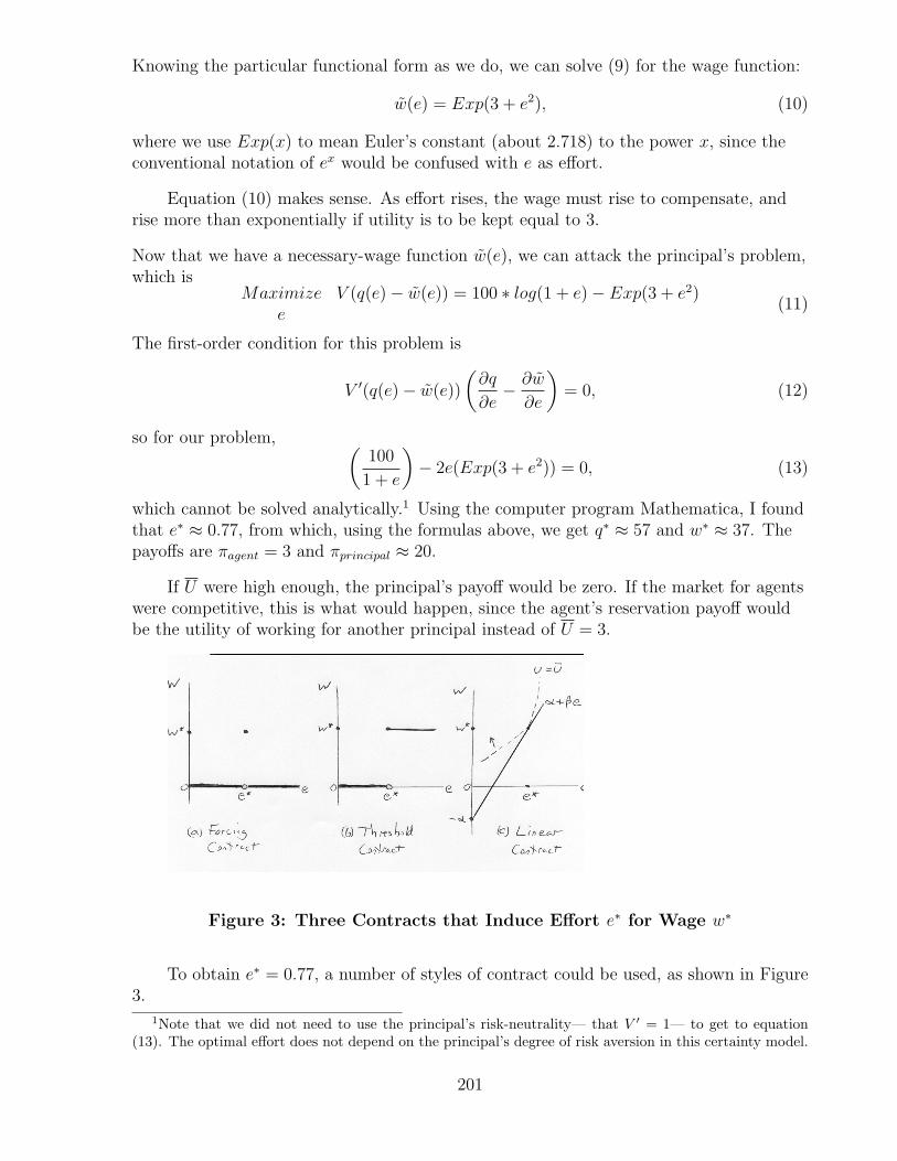
The principal selects the point on the U = U indifference curve that maximizes hisprofits, at effort e∗ and wage w∗. He must then design a contract that will induce theagent to choose this effort level. The following three contracts, shown in Figure 3, areequally effective under full information.

1 The forcing contract sets w(e∗) = w∗ and w(e 6= e∗) = 0. This is certainly a strongincentive for the agent to choose exactly e = e∗.

2 The threshold contract sets w(e ≥ e∗) = w∗ and w(e < e∗) = 0. This can be viewedas a flat wage for low effort levels, equal to 0 in this contract, plus a bonus if effortreaches e∗. Since the agent dislikes effort, the agent will choose exactly e = e∗.

3 The linear contract, shown in both Figure 2 and Figure 3(c), sets w(e) = α + βe,where α and β are chosen so that w∗ = α + βe∗ and the contract line is tangent to theindifference curve U = U at e∗. In Figure 3(c), the most northwesterly of the agent’sindifference curves that touch this contract line touches it at e∗.

Let’s now fit out Production Game I with specific functional forms. Suppose theagent exerts effort e ∈ [0,∞], and output equals

q(e) = 100 ∗ log(1 + e), (8)

so q′ = 1001+e

> 0 and q′′ = −100(1+e)2

< 0. If the agent rejects the contract, let πagent = U = 3and πprincipal = 0, whereas if the agent accepts the contract, letπagent = U(e, w) = log(w)− e2 and πprincipal = q(e)− w(e).

The agent must be paid some amount w(e) to exert effort e, where w(e) is defined tobe the wage that makes the agent willing to participate, i.e., as in equation (1),

U(e, w(e)) = U, so log(w(e))− e2 = 3. (9)

200

Knowing the particular functional form as we do, we can solve (9) for the wage function:

w(e) = Exp(3 + e2), (10)

where we use Exp(x) to mean Euler’s constant (about 2.718) to the power x, since theconventional notation of ex would be confused with e as effort.

Equation (10) makes sense. As effort rises, the wage must rise to compensate, andrise more than exponentially if utility is to be kept equal to 3.

Now that we have a necessary-wage function w(e), we can attack the principal’s problem,which is

Maximize V (q(e)− w(e)) = 100 ∗ log(1 + e)− Exp(3 + e2)e

(11)

The first-order condition for this problem is

V ′(q(e)− w(e))

(∂q

∂e− ∂w

∂e

)= 0, (12)

so for our problem, (100

1 + e

)− 2e(Exp(3 + e2)) = 0, (13)

which cannot be solved analytically.1 Using the computer program Mathematica, I foundthat e∗ ≈ 0.77, from which, using the formulas above, we get q∗ ≈ 57 and w∗ ≈ 37. Thepayoffs are πagent = 3 and πprincipal ≈ 20.

If U were high enough, the principal’s payoff would be zero. If the market for agentswere competitive, this is what would happen, since the agent’s reservation payoff wouldbe the utility of working for another principal instead of U = 3.

Figure 3: Three Contracts that Induce Effort e∗ for Wage w∗

To obtain e∗ = 0.77, a number of styles of contract could be used, as shown in Figure3.

1Note that we did not need to use the principal’s risk-neutrality— that V ′ = 1— to get to equation(13). The optimal effort does not depend on the principal’s degree of risk aversion in this certainty model.

201

1 The forcing contract sets w(e∗) = w∗ and w(e 6= 0.77) = 0. Here, w(0.77) = 37(rounding up) and w(e 6= e∗) = 0.

2 The threshold contract sets w(e ≥ e∗) = w∗ and w(e < e∗) = 0. Here,w(e ≥ 0.77) = 37 and w(e < 0.77) = 0.

3 The linear contract sets w(e) = α + βe, where α and β are chosen so thatw∗ = α + βe∗ and the contract line is tangent to the indifference curve U = U at e∗. Theslope of that indifference curve is the derivative of the w(e) function, which is

∂w(e)

∂e= 2e ∗ Exp(3 + e2). (14)

At e∗ = 0.77, this takes the value 56 (which only coincidentally is near the value ofq∗ = 57). That is the β for the linear contract. The α must solvew(e∗) = 37 = α + 56(0.77), so α = −7.

We ought to be a little concerned as to whether the agent will choose the effort wehope for if he is given the linear contract. We constructed it so that he would be willingto accept the contract, because if he chooses e = 0.77, his utility will be 3. But might heprefer to choose some larger or smaller e and get even more utility? No, because hisutility is concave. That makes the indifference curve convex, so its slope is alwaysincreasing and no preferable indifference curve touches the equilibrium contract line.

Quasilinearity and Alternative Functional Forms for the Production Game

Consider the following three functional forms for utility:

U(e, w) = log(w)− e2 (a)

U(e, w) = w − e2 (b)

U(e, w) = log(w − e2) (c)

(15)

Utility function (a) is what we just used in Production Game I. Utility function (b) is anexample of quasilinear preferences, because utility is separable in one good— money,here— and linear in that good. This kind of utility function is commonly used to avoidwealth effects that would otherwise occur in the interactions among the various goods inthe utility function. Separability means that giving an agent a higher wage does not, forexample, increase his marginal disutility of effort. Linearity means furthermore thatgiving an agent a higher wage does not change his tradeoff between money and effort, hismarginal rate of substitution, as it would in function (a), where a richer agent is lesswilling to accept money for higher effort. In effort-wage diagrams, quasilinearity impliesthat the indifference curves are parallel along the effort axis (which they are not in Figure2).

Quasilinear utility functions most often are chosen to look like (b), but my colleagueMichael Rauh points out that what quasilinearity really requires is just linearity in thespecial good (w here) for some monotonic transformation of the utility function. Utility

202

function (c) is a logarithmic transformation of (b), which is a monotonic transformation,so it too is quasilinear. That is because marginal rates of substitution, which is whatmatter here, are a feature of general utility functions, not the Von Neumann-Morgensternfunctions we typically use. Thus, utility function (c) is also a quasi-linear function,because it is just a monotonic function of (b). This is worth keeping in mind becauseutility function (c) is concave in w, so it represents a risk-averse agent.

Returning to the solution of Production Game I, let us now use a different approachto get to the same answer as we did using the principal’s maximization problem (11).Instead, we will return to the general optimality condition(6), here repeated.(

∂U

∂w

)(∂q

∂e

)= −∂U

∂e(6)

For any of our three utility functions we will continue using the same output functionq(e) = 100 ∗ log(1 + e) from (8), which has the first derivative q′ = 100

1+e.

Using utility function (a), ∂U∂w

= 1/w. and ∂U∂e

= −2e, so equation (6) becomes(1

w

)(100

1 + e

)= −(−2e). (16)

If we substitute for w using the function w(e) = Exp(3 + e2) that we found in equation(10), we get essentially the same equation as (13), and so outcomes are the same—e∗ ≈ 0.77, q∗ ≈ 57 , and w∗ ≈ 37, πagent = 3, and πprincipal ≈ 20.

Using utility function (b), ∂U∂w

= 1 and ∂U∂e

= −2e, so equation (6) becomes

(1)

(100

1 + e

)= − (−2e) (17)

Notice that w has disappeared. The optimal effort no longer depends on the agent’swealth. Thus, we don’t need to use the wage function to solve for the optimal effort.Solving directly, we get e∗ ≈ 6.59 and q∗ ≈ 203. The wage function will be different now,solving w − e2 = 3, so w∗ ≈ 43, πagent = 3, and πprincipal ≈ 160. (These numbers are notreally comparable to when we used utility function (a), but they will be useful inProduction Game II.)

Using utility function (c), ∂U∂w

= 1/(w − e2) and ∂U∂e

= −2e/(w − e2), so equation (6)becomes (

1

w − e2

)(100

1 + e

)= −

(−2e

w − e2

)(18)

and with a little simplification,100

1 + e= 2e. (19)

The variable w has again disappeared, so as with utility function (b) the optimal effortdoes not depend on the agent’s wealth. Solving for the optimal effort yields e∗ ≈ 6.59 andq∗ ≈ 203, the same as with utility function (b). The wage function is different, however.Now it solves log(w − e2) = 3, so w = e2 + exp(3) and w∗ ≈ 63, πagent = 3, andπprincipal ≈ 140.

203

Before going on to versions of the game with asymmetric information, it will beuseful to look at another version of the game with full information, Production Game II,in which the agent, not the principal, proposes the contract.

Production Game II: Full Information. Agent Moves First.

In this version, every move is common knowledge and the contract is a function w(e).The order of play, however, is now as follows

The Order of Play1 The agent offers the principal a contract w(e).2 The principal decides whether to accept or reject the contract.3 If the principal accepts, the agent exerts effort e.4 Output equals q(e), where q′ > 0.

Now the agent has all the bargaining power, not the principal. Thus, instead ofrequiring that the contract be at least barely acceptable to the agent, our concern is thatthe contract be at least barely acceptable to the principal, who must earn zero profits soq(e)− w(e) ≥ 0. The agent will maximize his own payoff by driving the principal toexactly zero profits, so w(e) = q(e). Substituting q(e) for w(e) to account for thisconstraint, the maximization problem for the agent in proposing an effort level e at awage w(e) can therefore be written as

Maximize U(e, q(e))e

(20)

The first-order condition is∂U

∂e+

(∂U

∂q

)(∂q

∂e

)= 0. (21)

Since ∂U∂q

= ∂U∂w

when the wages equals output, equation (21) implies that(∂U

∂w

)(∂q

∂e

)= −

(∂U

∂e

). (22)

Compare this with equation (6),the optimization condition in Production Game I, whenthe principal had the bargaining power, The optimality equation is identical inProduction Games I and II. The intuition is the same in both too: since the player whoproposes the contract captures all the gains from trade (for a given reservation payoff ofthe other player), he will choose an efficient effort level. This requires that the marginalutility of the money derived from marginal effort equal the marginal disutility of effort.

Although the form of the optimality equation is the same, however, the optimaleffort might not be, because except in the special case in which the agent’s reservationpayoff in Production Game I equals his equilibrium payoff in Production Game II, theagent ends up with higher wealth if he has all the bargaining power. If the utility functionis not quasi-linear, then the wealth effect will change the optimal effort.

We can see the wealth effect by solving out optimality equation (22) for the specificfunctional forms of Production Game I from expression (15).

204

Using utility function (a) from expression (15)(1

w

)(100

1 + e

)= −(−2e). (23)

That is the same as in Production Game I, equation (16), but now w is different. It is notfound by driving the agent to his reservation payoff, but by driving the principal to zeroprofits: w = q. Since q = 100 ∗ log(1 + e), we can substitute that in for w to get(

1

100 ∗ log(1 + e)

)(100

1 + e

)= 2e. (24)

When solved numerically, this yields e∗ ≈ 0.63, and thus q = w ≈ 49, and πprincipal = 0and πagent ≈ 3.49. In Production Game I, the optimal effort using this utility functionwas 0.77 and the agent’s payoff was 3. The difference arises because there the agent’swealth was lower because the principal had the bargaining power. In Production Game IIthe agent is, in effect, wealthier, and since his marginal utility of money is lower, hechooses to convert some (but not all) of that extra wealth into what we might callleisure— working less hard.

Using the quasilinear utility functions (b) and (c) from expression (15), recall thatboth have the same optimality condition, the one we found in equations (17) and (19):

100

1 + e= 2e (19)

As we observed before, w does not appear in equation (19), so the wage equation does notmatter to e∗. But that means that in Production Game II, e∗ ≈ 6.59 and q∗ ≈ 203, just asin Production Game I. With quasilinear utility, the efficient action does not depend onbargaining power. Of course, the wage and payoffs do depend on who has the bargainingpower. In Production Game II, w∗ = q∗ ≈ 203, and πprincipal = 0. The agent’s payoff ishigher than in Production Game I, but it differs, of course, depending on the payofffunction. For utility function (b) it is πagent ≈ 160 and for utility function (c) it isπagent ≈ 5.08.

If utility is quasilinear, the efficient effort level is independent of which side has thebargaining power because the gains from efficient production are independent of howthose gains are distributed so long as each party has no incentive to abandon therelationship. This as the same lesson as the Coase Theorem’s:, under general conditionsthe activities undertaken will be efficient and independent of the distribution of propertyrights (Coase [1960]). This property of the efficient-effort level means that the modeller isfree to make the assumptions on bargaining power that help to focus attention on theinformation problems he is studying.

There are thus three reasons why modellers so often use take-it-or-leave-it offers. Thefirst two reasons were discussed earlier in the context of Production Game I: (1) suchoffers are a good way to model competitive markets, and (2) if the reservation payoff ofthe player without the bargaining power is set high enough, such offers lead to the sameoutcome as would be reached if that player had more bargaining power. Quasi-linearutility provides a third reason: (3) if utility is quasi-linear, the optimal effort level does

205

not depend on who has the bargaining power, so the modeller is justified in choosing thesimplest model of bargaining.

Production Game III: A Flat Wage Under Certainty

In this version of the game, the principal can condition the wage neither on effort noron output. This is modelled as a principal who observes neither effort nor output, soinformation is asymmetric.

That a principal cannot observe effort is often realistic, but it seems less usual thathe cannot observe output, since it directly affects the value of his payoff. It is notridiculous that he cannot base wages on output, however, because a contract must beenforceable by some third party such as a court. Law professors complain abouteconomists who speak of “unenforceable contracts.” In law school, a contract is defined asan enforceable agreement, and most of a contracts class is devoted to discovering whichagreements are contracts. A court cannot in practice enforce a contract in which a clientagrees to pay a barber $50 “if the haircut is especially good,” but just $10 otherwise.Similarly, an employer may be able to tell that a worker’s slacking is hurting output, butthat does not mean he can prove it in court. A court can only enforce contingencies it canobserve. In the extreme, Production Game III is appropriate. Either output is notcontractible (the court will not enforce a contract) or it is not verifiable (the courtcannot observe output), which usually leads to the same outcome as when output isunobservable to the principal.

The outcome of Production Game III is simple and inefficient. If the wage isnonnegative, the agent accepts the job and exerts zero effort, so the principal offers awage of zero.

In Production Game III, we have finally reached “moral hazard”, the problem of theagent choosing the wrong action because the principal cannot use the contract to punishhim. The term “moral hazard” is an old insurance term, as we will see later. A good wayto think of it is that it is the danger to the principal that the agent, constrained only byhis morality, not punishments, cannot be trusted to behave as he ought. Or, you mightthink of the situation as a temptation for the agent, a hazard to his morals.

Sometimes, as we will soon see, a clever contract can overcome moral hazard byconditioning the wage on something that is observable and correlated with effort, such asoutput. If there is nothing on which to condition the wage, however, the agency problemcannot be solved by designing the contract carefully. If it is to be solved at all, it will beby some other means such as reputation or repetition of the game, the solutions ofChapter 5, or by morality– which might be modelled as a part of the agent’s utilityfunction which causes him disutility if he secretly breaks an agreement. Typically,however, there is some contractible variable such as output upon which the principal cancondition the wage. Such is the case in Production Game IV.

Production Game IV: An Output-Based Wage under Certainty

In this version, the principal cannot observe effort but he can observe output and

206

specify the contract to be w(q).

Unlike in Production Game III, the principal now picks not a number w but afunction w(q). His problem is not quite so straightforward as in Production Game I, wherehe picked the function w(e), but here, too, it is possible to achieve the efficient effort levele∗ despite the unobservability of effort. The principal starts by finding the optimal effortlevel e∗, as in Production Game I. That effort yields the efficient output level q∗ = q(e∗).To give the agent the proper incentives, the contract must reward him when output is q∗.Again, a variety of contracts could be used. The forcing contract, for example, would beany wage function such that U(e∗, w(q∗)) = U and U(e, w(q)) < U for e 6= e∗.

Production Game IV shows that the unobservability of effort is not a problem initself, if the contract can be conditioned on something which is observable and perfectlycorrelated with effort. The true agency problem occurs when that perfect correlationbreaks down, as in Production Game V.

Production Game V: An Output-Based Wage under Uncertainty.

In this version, the principal cannot observe effort but can observe output andspecify the contract to be w(q). Output, however, is a function q(e, θ) both of effort andthe state of the world θ ∈ R, which is chosen by Nature according to the probabilitydensity f(θ) as a new move (5) of the game. Move (5) comes just after the agent chooseseffort, so the agent cannot choose a low effort knowing that Nature will take up the slack.(If the agent can observe Nature’s move before his own, the game becomes “moral hazardwith hidden knowledge and hidden actions”).

Because of the uncertainty about the state of the world, effort does not map cleanlyonto observed output in Production Game V. A given output might have been producedby any of several different effort levels, so a forcing contract based on output will notnecessarily achieve the desired effort. Unlike in Production Game IV, here the principalcannot deduce e 6= e∗ from q 6= q∗. Moreover, even if the contract does induce the agentto choose e∗, if it does so by penalizing him heavily when q 6= q∗ it will be expensive forthe principal. The agent’s expected utility must be kept equal to U so he will accept thecontract, and if he is sometimes paid a low wage because output happens not to equal q∗

despite his correct effort, he must be paid more when output does equal q∗ to make up forit. If the agent is risk averse, this variability in his wage requires that his expected wagebe higher than the w∗ found earlier, because he must be compensated for the extra risk.There is a tradeoff between incentives and insurance against risk.

Put more technically, moral hazard is a problem when q(e) is not a one-to- onefunction and a single value of e might result in any of a number of values of q, dependingon the value of θ. In this case the output function is not invertible; knowing q, theprincipal cannot deduce the value of e perfectly without assuming equilibrium behavioron the part of the agent.

The combination of unobservable effort and lack of invertibility in Production GameV means that no contract can induce the agent to put forth the efficient effort levelwithout incurring extra costs, which usually take the form of extra risk imposed on the

207

agent. In some situations this is not actually a cost, because the agent is risk-neutral, butmore often the best the principal can do is balance the benefit of extra incentive for effortagainst the cost of extra risk for a risk-average agent. We will still try to find a contractthat is efficient in the sense of maximizing welfare given the informational constraints.The terms “first-best” and “second-best” are used to distinguish these two kinds ofoptimality.

A first-best contract achieves the same allocation as the contract that is optimal whenthe principal and the agent have the same information set and all variables arecontractible.

A second-best contract is Pareto optimal given information asymmetry and constraintson writing contracts.

The difference in welfare between the first best and the second best is the cost of theagency problem.

So how do we find a second-best contract? Even to define the strategy space in agame like Production Game V is tricky, because the principal may wish to choose a verycomplicated function for w(q). It is not very useful, for example, simply to maximizeprofit over all possible linear contracts, because the best contract may well not be linear.Because of the tremendous variety of possible contracts, finding the optimal contractwhen a forcing contract cannot be used is a hard problem without general answers. Therest of the chapter will show how the problem may be approached, if not actually solved.

7.3 The Incentive Compatibility and Participation Constraints

The principal’s objective in Production Game V is to maximize his utility knowingthat the agent is free to reject the contract entirely and that the contract must give theagent an incentive to choose the desired effort. These two constraints arise in every moralhazard problem, and they are named the participation constraint and the incentivecompatibility contraint. Mathematically, the principal’s problem is

Maximize EV (q(e, θ)− w(q(e, θ)))w(·) (25)

subject to

e =argmax

e EU(e, w(q(e, θ))) (incentive compatibility constraint) (25a)

EU(e, w(q(e, θ))) ≥ U (participation constraint) (25b)

The incentive-compatibility constraint takes account of the fact that the agent movessecond, so the contract must induce him to voluntarily pick the desired effort. The

208

participation constraint, also called the reservation utility or individual rationalityconstraint, requires that the worker prefer the contract to leisure, home production, oralternative jobs.

Expression (25) is the way an economist instinctively sets up the problem, butsetting it up is often as far as he can get with the first- order condition approach.The difficulty is not just that the maximizer is choosing a wage function instead of anumber, because control theory or the calculus of variations can solve such problems.Rather, it is that the constraints are nonconvex— they do not rule out a nice convex setof points in the space of wage functions such as the constraint “w ≥ 4” would, but ratherrule out a very complicated set of possible wage functions.

A different approach, developed by Grossman & Hart (1983) and called thethree-step procedure by Fudenberg & Tirole (1991a), is to focus on contracts thatinduce the agent to pick a particular action rather than to directly attack the problem ofmaximizing profits. The first step is to find for each possible effort level the set of wagecontracts that induce the agent to choose that effort level. The second step is to find thecontract which supports that effort level at the lowest cost to the principal. The thirdstep is to choose the effort level that maximizes profits, given the necessity to supportthat effort with the costly wage contract from the second step.

To support the effort level e, the wage contract w(q) must satisfy the incentivecompatibility and participation constraints. Mathematically, the problem of finding theleast cost C(e) of supporting the effort level e combines steps one and two.

C(e) = Minimum Ew(q(e, θ))w(·) (26)

subject to constraints (25a) and (25b).

Step three takes the principal’s problem of maximizing his payoff, expression (25),and restates it as

Maximize EV (q(e, θ)− C(e)).e

(27)

After finding which contract most cheaply induces each effort, the principal discovers theoptimal effort by solving problem (27).

Breaking the problem into parts makes it easier to solve. Perhaps the mostimportant lesson of the three-step procedure, however, is to reinforce the points that thegoal of the contract is to induce the agent to choose a particular effort level and thatasymmetric information increases the cost of the inducements.

7.4 Optimal Contracts: The Broadway Game

The next game, inspired by Mel Brooks’s offbeat film The Producers, illustrates a

209

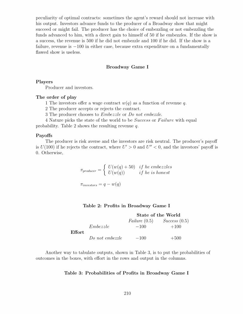
peculiarity of optimal contracts: sometimes the agent’s reward should not increase withhis output. Investors advance funds to the producer of a Broadway show that mightsucceed or might fail. The producer has the choice of embezzling or not embezzling thefunds advanced to him, with a direct gain to himself of 50 if he embezzles. If the show isa success, the revenue is 500 if he did not embezzle and 100 if he did. If the show is afailure, revenue is −100 in either case, because extra expenditure on a fundamentallyflawed show is useless.

Broadway Game I

PlayersProducer and investors.

The order of play1 The investors offer a wage contract w(q) as a function of revenue q.2 The producer accepts or rejects the contract.3 The producer chooses to Embezzle or Do not embezzle.4 Nature picks the state of the world to be Success or Failure with equal

probability. Table 2 shows the resulting revenue q.

PayoffsThe producer is risk averse and the investors are risk neutral. The producer’s payoff

is U(100) if he rejects the contract, where U ′ > 0 and U ′′ < 0, and the investors’ payoff is0. Otherwise,

πproducer =

{U(w(q) + 50) if he embezzlesU(w(q)) if he is honest

πinvestors = q − w(q)

Table 2: Profits in Broadway Game I

State of the WorldFailure (0.5) Success (0.5)

Embezzle −100 +100Effort

Do not embezzle −100 +500

Another way to tabulate outputs, shown in Table 3, is to put the probabilities ofoutcomes in the boxes, with effort in the rows and output in the columns.

Table 3: Probabilities of Profits in Broadway Game I

210

Profit-100 +100 +500 Total

Embezzle 0.5 0.5 0 1Effort

Do not embezzle 0.5 0 0.5 1

The investors will observe q to equal either −100, +100, or +500, so the producer’scontract will specify at most three different wages: w(−100), w(+100), and w(+500). Theproducer’s expected payoffs from his two possible actions are

π(Do not embezzle) = 0.5U(w(−100)) + 0.5U(w(+500)) (28)

andπ(Embezzle) = 0.5U(w(−100) + 50) + 0.5U(w(+100) + 50). (29)

The incentive compatibility constraint is π(Do not embezzle) ≥ π(Embezzle), so

0.5U(w(−100)) + 0.5U(w(+500)) ≥ 0.5U(w(−100) + 50) + 0.5U(w(+100) + 50), (30)

and the participation constraint is

π(Do not embezzle) = 0.5U(w(−100)) + 0.5U(w(+500)) ≥ U(100). (31)

The investors want the participation constraint (31) to be satisfied at as low a dollar costas possible. This means they want to impose as little risk on the producer as possible,since he requires a higher expected wage for higher risk. Ideally, w(−100) = w(+500),which provides full insurance. The usual agency tradeoff is between smoothing out theagent’s wage and providing him with incentives. Here, no tradeoff is required, because ofa special feature of the problem: there exists an outcome that could not occur unless theproducer chooses the undesirable action. That outcome is q = +100, and it means thatthe following boiling-in-oil contract provides both riskless wages and effectiveincentives.

w(+500) = 100w(−100) = 100w(+100) = −∞

Under this contract, the producer’s wage is a flat 100 when he does not embezzle.Thus, the participation constraint is satisfied. It is also binding, because it is satisfied asan equality, and the investors would have a higher payoff if the constraint were relaxed. Ifthe producer does embezzle, he faces a payoff of −∞ with probability 0.5, so the incentivecompatibility constraint is satisfied, but it is nonbinding, because it is satisfied as a stronginequality and the investors’ equilibrium payoff does not fall if the constraint is tighteneda little by making the producer’s earnings from embezzlement slightly higher. The cost ofthe contract to the investors is 100 in equilibrium, so their overall expected payoff is0.5(−100) + 0.5(+500)− 100 = 100, an amount greater than zero and thus yieldingenough return for the show to be profitable.

The boiling-in-oil contract is an application of the sufficient statistic condition,which says that for incentive purposes, if the agent’s utility function is separable in effort

211

and money, wages should be based on whatever evidence best indicates effort, and onlyincidentally on output (see Holmstrom [1979] and note N7.2). In the spirit of thethree-step procedure, what the principal wants is to induce the agent to choose theappropriate effort, Do not embezzle, and his data on what the agent chose is the output.In equilibrium (though not out of it), the datum q = +500 contains exactly the sameinformation as the datum q = −100. Both lead to the same posterior probability that theagent chose Do not embezzle, so the wages conditioned on each datum should be thesame. We need to insert the qualifier “in equilibrium,” because to form the posteriorprobabilities the principal needs to have some beliefs as to the agent’s behavior.Otherwise, the principal could not interpret q = −100 at all.

Milder contracts would also be effective. Two wages will be used in equilibrium, alow wage w for an output of q = 100 and a high wage w for any other output. Theparticipation and incentive compatibility constraints provide two equations to solve forthese two unknowns. To find the mildest possible contract, the modeller must also specifya function for utility U(w), something which, interestingly enough, was unnecessary forfinding the first boiling-in-oil contract. Let us specify that

U(w) = 100w − 0.1w2. (32)

A quadratic utility function like this is only increasing if its argument is not too large,but since the wage will not exceed w = 1000, it is a reasonable utility function for thismodel. Substituting (32) into the participation constraint (31) and solving for thefull-insurance high wage w = w(−100) = w(+500) yields w = 100 and a reservationutility of 9000. Substituting into the incentive compatibility constraint, (30), yields

9000 ≥ 0.5U(100 + 50) + 0.5U(w + 50). (33)

When (33) is solved using the quadratic equation, it yields (with rounding error),w ≤ 5.6. A low wage of −∞ is far more severe than what is needed.

If both the producer and the investors were risk averse, risk sharing would changethe part of the contract that applied in equilibrium. The optimal contract would thenprovide for w(−100) < w(+500) to share the risk. The principal would have a lowermarginal utility of wealth when output was +500, so he would be better able to pay anextra dollar of wages in that state than when output was −100.

One of the oddities of Broadway Game I is that the wage is higher for an output of−100 than for an output of +100. This illustrates the idea that the principal’s aim is toreward input, not output. If the principal pays more simply because output is higher, heis rewarding Nature, not the agent. People usually believe that higher pay for higheroutput is “fair,” but Broadway Game I shows that this ethical view is too simple. Highereffort usually leads to higher output, but not always. Thus, higher pay is usually a goodincentive, but not always, and sometimes low pay for high output actually punishesslacking.

The decoupling of reward and result has broad applications. Becker (1968) incriminal law and Polinsky & Che (1991) in tort law note that if society’s objective is to

212

keep the amount of enforcement costs and harmful behavior low, the penalty appliedshould not simply be matched to the harm. Very high penalties seldom inflicted willprovide the proper incentives and keep enforcement costs low, even though a few unluckyoffenders will receive penalties out of proportion to the harm they caused.

A less gaudy name for a boiling-in-oil contract is the alliterative “shifting supportscheme,” so named because the contract depends on the support of the outputdistribution being different when effort is optimal than when effort is other than optimal.The set of possible outcomes under optimal effort must be different from the set ofpossible outcomes under any other effort level. As a result, certain outputs show withoutdoubt that the producer embezzled. Very heavy punishments inflicted only for thoseoutputs achieve the first-best because a non-embezzling producer has nothing to fear.

Figure 4: Shifting Supports in an Agency Model

Figure 4a shows shifting supports in a model where output can take not three but acontinuum of values. If the agent shirks instead of working, certain low outputs becomepossible and certain high outputs become impossible. In a case like this, where thesupport of the output shifts when behavior changes, boiling-in-oil contracts are useful:the wage is −∞ for the low outputs possible only under shirking. In Figure 4b, on theother hand, the support just shrinks under shirking, so boiling in oil is inappropriate.When there is a limit to the amount the agent can be punished, or the support undershirking is a subset of the first-best support, the threat of boiling-in-oil might not achievethe first-best. Sometimes, however, similar contracts can still be used. The conditionsfavoring such contracts are

1 The agent is not very risk averse.

2 There are outcomes with high probability under shirking that have low probabilityunder optimal effort.

3 The agent can be severely punished.

4 It is credible that the principal will carry out the severe punishment.

Selling the Store

Another first-best contract that can sometimes be used is selling the store. Under thisarrangement, the agent buys the entire output for a flat fee paid to the principal,

213

becoming the residual claimant, since he keeps every additional dollar of output thathis extra effort produces. This is equivalent to fully insuring the principal, since his payoffbecomes independent of the moves of the agent and of Nature.

In Broadway Game I, selling the store takes the form of the producer paying theinvestors 100 (= 0.5[−100] + 0.5[+500]− 100) and keeping all the profits for himself. Thedrawbacks are that (1) the producer might not be able to afford to pay the investors theflat price of 100; and (2) the producer might be risk averse and incur a heavy utility costin bearing the entire risk. These two drawbacks are why producers go to investors in thefirst place.

Public Information that Hurts the Principal and the Agent

We can modify Broadway Game I to show how having more public information availablecan hurt both players. This will also provide a little practice in using information sets.Let us split Success into two states of the world, Minor Success and Major Success,which have probabilities 0.3 and 0.2 as shown in Table 4.

Table 4: Profits in Broadway Game II

State of the WorldFailure (0.5) Minor Success (0.3) Major Success (0.2)

Embezzle −100 −100 +400Effort

Do not embezzle −100 +450 +575

Under the optimal contract,

w(−100) = w(+450) = w(+575) > w(+400) + 50. (34)

This is so because the producer is risk averse and only the datum q = +400 is proofthat the producer embezzled. The optimal contract must do two things: deterembezzlement and pay the producer as predictable a wage as possible. For predictability,the wage is made constant unless q = +400. To deter embezzlement, the producer mustbe punished if q = +400. As in Broadway Game I, the punishment would not have to beinfinitely severe, and the minimum effective punishment could be calculated in the sameway as in that game. The investors would pay the producer a wage of 100 in equilibriumand their expected payoff would be 100 (= 0.5(−100) + 0.3(450) + 0.2(575)− 100). Thus,a contract can be found for Broadway Game II such that the agent would not embezzle.

But consider what happens when the information set is refined so that before theagent takes his action both he and the principal can tell whether the show will be a majorsuccess or not. Let us call this Broadway Game III. Under the refinement, each player’sinformation partition is

({Failure, Minor Success}, {Major Success}),

214

instead of Broadway Game I and II’s coarse partition

({Failure, Minor Success, Major Success}).

If the information sets were refined all the way to singletons, this would be very useful tothe investors, because they could abstain from investing in a failure and they could easilydetermine whether the producer embezzled or not. As it is, however, the refinement doesnot help the investors decide when to finance the show. If they could still hire theproducer and prevent him from embezzling at a cost of 100, the payoff from investing in amajor success would be 475 (= 575− 100). But the payoff from investing in a show giventhe information set {Failure, Minor Success} would be about 6.25, which is still positive((

0.50.5+0.3

)(−100) +

(0.3

0.5+0.3

)(450)− 100). So the improvement in information is no help

with respect to the decision of when to invest.

The refinement does, however, ruin the producer’s incentives. If he observes{Failure, Minor Success}, he is free to embezzle without fear of the oil-boiling output of+400. He would still refrain from embezzling if he observed {Major Success}, but nocontract that does not impose risk on a nonembezzling producer can stop him fromembezzling if he observes {Failure, Minor Success}. Whether a risky contract can befound that would prevent the producer from embezzling at a cost of less than 6.25 to theinvestors depends on the producer’s risk aversion. If he is very risk averse, the cost of theincentive is more than 6.25, and the investors will give up investing in shows that mightbe minor successes. Better information reduces welfare, because it increases theproducer’s temptation to misbehave.

215

Notes

N7.1 Categories of Asymmetric Information Models

• Three books that cover the theory of contracts are Macho-Stadler and Perez- Castillo’s1997 An Introduction to the Economics of Information: Incentives and Contracts,Salanie’s 1997 The Economics of Contracts: A Primer and Bolton and Dewatripont’s2005 Contract Theory. For a survey of recent empirical work on contracts, see Chiappori,P.A. & B. Salanie (2003).

• A large literature of nonmathematical theoretical papers looks at organizational structurein the light of the agency problem. See Alchian & Demsetz (1972), Fama (1980), andKlein, Crawford, & Alchian (1978). Milgrom & Roberts (1992) have written a book onorganization theory that describes what has been learned about the principal-agentproblem at a technical level that MBA students can understand. There may be much tobe learned from intelligent economists of the past also; note that part III, chapter 8,section 12 of Pigou’s Economics of Welfare (1932/1920) has an interesting discussion ofthe advantage of piece-rate work, which can more easily induce each worker to choose thecorrect effort when abilities differ as well as efforts. I recommend Chapter 1 (“Incentivesin Economic Thought”) of Laffont & Martimort (2002) as a short survey of the history ofincentives in economic theory.

• An important consideration in real-world contracts is manipulation and fraud by theagent. If an executive is rewarded for higher earnings per share, and he controls theaccountants who measure earnings, for example, he may tell them to measure them sothat they surpass the threshold in his threshold contract. Even worse, he might cut pricesso as to speed up sales before January 1 and meet his yearly target. Jensen’s 2003“Paying People To Lie: The Truth about the Budgeting Process,” points this out andnotes that linear contracts are less vulnerable to this type of manipulation.

• We have lots of “prinsipuls” in economics. I find this paradigm helpful for rememberingspelling: “The principal’s principal principle was to preserve his principal.” More simply,“The principal is my pal,” takes care of the “al” case.

• “Principal” and “Agent” are legal terms, and agency is an important area of the law.Economists have focussed on quite different questions than lawyers. Economists focus oneffort: how the principal induces the agent to do things. Lawyers focus on malfeasanceand third parties: how the principal stops the agent from doing the wrong things and whobears the burden if he fails. If, for example, the manager of a tavern enters into a supplycontract against the express command of the owner, who must be disappointed— theowner or the third party supplier?

• Double-sided moral hazard. The text described one-sided moral hazard. Moral hazard canalso be double-sided, as when each player takes actions unobservable by the other thataffect the payoffs of both of them. An example is tort negligence by both plaintiff anddefendant: if a careless auto driver hits a careless pedestrian, and they go to law, thecourt must try to allocate blame, and the legislature must try to set up laws to induce theproper amount of care. Landlords and tenants also face double moral hazard, as impliedin Table 1.

• A common convention in principal-agent models is to make one player male and the otherfemale, so that “his” and “her” can be used to distinguish between them. I find this

216

distracting, since gender is irrelevant to most models and adds one more detail for thereader to keep track of. If readers naturally thought “male” when they saw “principal,”this would not be a problem— but they do not.

N7.2 A Principal-Agent Model: The Production Game

• The model in the text uses “effort” as the action taken by the agent, but effort is used torepresent a variety of real-world actions. The cost of pilferage by employees is anestimated $8 billion a year in the USA. Employers have offered rewards for detection, oneeven offering the option of a year of twice-weekly lottery tickets instead of a lump sum.The Chicago department store Marshall Field’s, with 14,000 workers, in one year gave out170 rewards of $500 each, catching almost 500 dishonest employees. (“Hotlines and HeftyRewards: Retailers Step Up Efforts to Curb Employee Theft,” Wall Street Journal,September 17,1987, p. 37.)

For an illustration of the variety of kinds of “low effort,” see “Hermann Hospital Estate,Founded for the Poor, Has Benefited the Wealthy, Investigators Allege,” Wall StreetJournal, March 13, 1985, p. 4, which describes such forms of misbehavior as pleasure tripson company funds, high salaries, contracts for redecorating awarded to girlfriends, phonychecks, kicking back real estate commissions, and investing in friendly companies.Nonprofit enterprises, often lacking both principles and principals, are especiallyvulnerable, as are governments, for the same reason.

• The Production Game assumes that the agent dislikes effort. Is this realistic? Peoplediffer. My father tells of his experience in the navy when the sailors were kept busy bybeing ordered to scrape loose paint. My father found it a way to pass the time but saysthat other sailors would stop chipping when they were not watched, preferring to stareinto space. De gustibus non est disputandum (“About tastes there can be no arguing”).But even if effort has positive marginal utility at low levels, it has negative marginalutility at high enough levels— including, perhaps, at the efficient level. This is as true forprofessors as for sailors.

• Suppose that the principal does not observe the variable θ (which might be effort), but hedoes observe t and x (which might be output and profits). From Holmstrom (1979) andShavell (1979) we have, restated in my words,

The Sufficient Statistic Condition. If t is a sufficient statistic for θ relative to x, thenthe optimal contract needs to be based only on t if both principal and agent have separableutility functions.

The variable t is a sufficient statistic for θ relative to x if, for all t and x,

Prob(θ|t, x) = Prob(θ|t). (35)

This implies, from Bayes’ Rule, that Prob(t, x|θ) = Prob(x|t)Prob(t|θ); that is, x dependson θ only because x depends on t and t depends on θ.

The sufficient statistic condition is closely related to the Rao- Blackwell Theorem (seeCox & Hinkley [1974] p. 258), which says that the decision rule for nonstrategic decisionsought not to be random.

217

Gjesdal (1982) notes that if the utility functions are not separable, the theorem doesnot apply and randomized contracts may be optimal. Suppose there are two actions theagent might take. The principal prefers action X, which reduces the agent’s risk aversion,to action Y , which increases it. The principal could offer a randomized wage contract, sothe agent would choose action X and make himself less risk averse. This randomization isnot a mixed strategy. The principal is not indifferent to high and low wages; he prefers topay a low wage, but we allow him to commit to a random wage earlier in the game.

N7.3 The Incentive Compatibility and Participation Constraints

• The term, “individual rationality constraint,” is perhaps more common, but“participation constraint” is more sensible. Since in modern modelling every constraintrequires individuals to be rational, the name is ill-chosen.

• Paying the agent more than his reservation wage. If agents compete to work forprincipals, the participation constraint is binding whenever there are only two possibleoutcomes or whenever the agent’s utility function is separable in effort and wages.Otherwise, it might happen that the principal picks a contract giving the agent moreexpected utility than is necessary to keep him from quitting. The reason is that theprincipal not only wants to keep the agent working, but to choose a high effort.

• If the distribution of output satisfies the monotone likelihood ratio property(MLRP), the optimal contract specifies higher pay for higher output. Let f(q|e) be theprobability density of output. The MLRP is satisfied if

∀e′ > e, and q′ > q, f(q′|e′)f(q|e)− f(q′|e)f(q|e′) > 0, (36)

or, in other words, if when e′ > e, the ratio f(q|e′)/f(q|e) is increasing in q. Alternatively,f satisfies the MLRP if q′ > q implies that q′ is a more favorable message than q in thesense of Milgrom (1981b). Less formally, the MLRP is satisfied if the ratio of thelikelihood of a high effort to a low effort rises with observed output. The distributions inThe Broadway Game of Section 7.4 violate the MLRP, but the normal, exponential,Poisson, uniform, and chi-square distributions all satisfy it. Stochastic dominance doesnot imply the MLRP. If effort of 0 produces outputs of 10 or 12 with equal probability,and effort of 1 produces outputs of 11 or 13 also with equal probability, the seconddistribution is stochastically dominant, but the MLRP is not satisfied. See Chapter 13(Auctions) for more on the MLRP.

N7.4 Optimal Contracts: The Broadway Game

• Daniel Asquith suggested the idea behind Broadway Game II.

• Franchising is one compromise between selling the store and paying a flat wage. SeeMathewson & Winter (1985), Rubin (1978), and Klein & Saft (1985).

• Mirrlees (1974) is an early reference on the idea of the boiling-in-oil contract.

218

• Broadway Game II shows that improved information could reduce welfare by increasing aplayer’s incentive to misbehave. This is distinct from the nonstrategic insurance reasonwhy improved information can be harmful. Suppose that Smith is insuring Jones againsthail ruining Jones’ wheat crop during the next year, increasing Jones’ expected utility andgiving a profit to Smith. If someone comes up with a way to forecast the weather beforethe insurance contract is agreed upon, both players will be hurt. Insurance will breakdown, because if it is known that hail will ruin the crop, Smith will not agree to share theloss, and if it is known there will be no hail, Jones will not pay a premium for insurance.Both players prefer not knowing the outcome in advance.

219

Problems

7.1: First-Best Solutions in a Principal-Agent Model (easy)Suppose an agent has the utility function of U =

√w − e, where e can assume the levels 0

or 1. Let the reservation utility level be U = 3. The principal is risk neutral. Denote the agent’swage, conditioned on output, as w if output is 0 and w if output is 100. Table 5 shows theoutputs.

Table 5: A Moral Hazard Game

Probability of Output ofEffort 0 100 Total

Low (e = 0) 0.3 0.7 1

High (e = 1) 0.1 0.9 1

(a) What would the agent’s effort choice and utility be if he owned the firm?

(b) If agents are scarce and principals compete for them, what will the agent’s contract beunder full information? His utility?

(c) If principals are scarce and agents compete to work for them, what would the contract beunder full information? What will the agent’s utility and the principal’s profit be in thissituation?

(d) Suppose that U = w − e. If principals are the scarce factor and agents compete to workfor principals, what would the contract be when the principal cannot observe effort?(Negative wages are allowed.) What will be the agent’s utility and the principal’s profit bein this situation?

7.2: The Principal-Agent Problem (medium)Suppose the agent has a utility function of U =

√w − e, where e can assume the levels 0 or

7, and a reservation utility of U = 4. The principal is risk neutral. Denote the agent’s wage,conditioned on output, as w if output is 0 and w if output is 1,000. Only the agent observes hiseffort. Principals compete for agents. Table 6 shows the output.

Table 6: Output from Low and High Effort

Probability of output ofEffort 0 1,000 Total

Low(e = 0) 0.9 0.1 1

High (e = 7) 0.2 0.8 1

220

(a) What are the incentive compatibility, participation, and zero- profit constraints forobtaining high effort?

(b) What would utility be if the wage were fixed and could not depend on output or effort?

(c) What is the optimal contract? What is the agent’s utility?

(d) What would the agent’s utility be under full information? Under asymmetric information,what is the agency cost (the lost utility) as a percentage of the utility the agent receives?

7.3. Why Entrepreneurs Sell Out (medium)Suppose an agent has a utility function of U =

√w − e, where e can assume the levels 0 or

2.4, and his reservation utility is U = 7. The principal is risk neutral. Denote the agent’s wage,conditioned on output, as w(0), w(49), w(100), or w(225). Table 7 shows the output.

Table 7: Entrepreneurs Selling Out

Probability of output ofMethod 0 49 100 225 Total

Safe (e = 0) 0.1 0.1 0.8 0 1

Risky (e = 2.4) 0 0.5 0 0.5 1

(a) What would the agent’s effort choice and utility be if he owned the firm?

(b) If agents are scarce and principals compete for them, what will the agent’s contract beunder full information? His utility?

(c) If principals are scarce and agents compete to work for principals, what will the contractbe under full information? What will the agent’s utility and the principal’s profit be inthis situation?

(d) If agents are the scarce factor, and principals compete for them, what will the contract bewhen the principal cannot observe effort? What will the agent’s utility and the principal’sprofit be in this situation?

7.4. Authority (medium)A salesman must decide how hard to work on his own time on getting to know a potential

customer. If he exerts effort X, he incurs a utility cost X2/2. With probability X, he can thengo to customer X and add V to his own earnings. With probability (1-X), he offends thecustomer, and on going to him would subtract L from his earnings. The boss will receive benefitB from the sale in either case. The ranking of these numbers is V > L > B > 0. The boss andthe salesman have equal bargaining power, and are free to make side payments to each other.

(a) What is the first-best level of effort, Xa?

221

(b) If the boss has the authority to block the salesman from selling to this customer, butcannot force him to sell, what value will X take?

(c) If the salesman has the authority over the decision on whether to sell to this customer,and can bargain for higher pay, what will his effort be?

(d) Rank the effort levels Xa, Xb, and Xc in the previous three sections.

7.5. Worker Effort (easy)A worker can be Careful or Careless, efforts which generate mistakes with probabilities

0.25 and 0.75. His utility function is U = 100− 10/w − x, where w is his wage and x takes thevalue 2 if he is careful, and 0 otherwise. Whether a mistake is made is contractible, but effort isnot. Risk-neutral employers compete for the worker, and his output is worth 0 if a mistake ismade and 20 otherwise. No computation is needed for any part of this problem.

(a) Will the worker be paid anything if he makes a mistake?

(b) Will the worker be paid more if he does not make a mistake?

(c) How would the contract be affected if employers were also risk averse?

(d) What would the contract look like if a third category, “slight mistake,” with an output of19, occurs with probability 0.1 after Careless effort and with probability zero afterCareful effort?

7.6. The Supercomputer Salesman (medium)If a salesman exerts high effort, he will sell a supercomputer this year with probability 0.9.

If he exerts low effort, he will succeed with probability 0.5. The company will make a profit of 2million dollars if the sale is made. The salesman would require a wage of $50,000 if he had toexert low effort, but $70,000 if he had to exert high effort, he is risk neutral, and his utility isseparable in effort and money. (Let’s just use payoffs in thousands of dollars, so 70,000 dollarswill be written as 70, and 2 million dollars will be 2000)

(a) Prove that high effort is first-best efficient.

(b) How high would the probability of success with low effort have to be for high effort to beinefficient?

(c) If you cannot monitor the programmer and cannot pay him a wage contingent on success,what should you do?

(d) Now suppose you can make the wage contingent on success. Let the wage be S if he makesa sale and F if he does not. S and F will have to satisfy two conditions: a participationconstraint and an incentive compatibility constraint. What are they?

(e) What is a contract that will achieve the first best?

(f) Now suppose the salesman is risk averse, and his utility from money is log(w). Set up theparticipation and incentive compatibility constraints again.

222

(g) You do not need to solve for the optimal contract. Using the log(w) utility functionassumption, however, will the expected payment by the firm in the optimal contract rise,fall, or stay the same, compared with what it was in part (e) for the risk neutral salesman?

(h) You do not need to solve for the optimal contract. Using the log(w) utility functionassumption, however, will the gap between S and F in the optimal contract rise, fall, orstay the same, compared with what it was in part (e) for the risk neutral salesman?

7.7. Optimal Compensation (easy)An agent’s utility function is U =(log(wage) - effort). What should his compensation

scheme be if different (output,effort) pairs have the probabilities in Table 8?(a) The agent should be paid exactly his output.(b) The same wage should be paid for outputs of 1 and 100.(c) The agent should receive more for an output of 100 than of 1, but should receive still

lower pay if output is 2.(d) None of the above.

Table 8: Output Probabilities

Output1 2 100

High 0.5 0 0.5Effort

Low 0.1 0.8 0.1

7.8. Effort and Output, Multiple Choices (easy)The utility function of the agents whose situation is depicted in Table 9 is

U = w +√

w − αe, and his reservation utility is 0. Principals compete for agents, and havereservation profits of zero. Principals are risk neutral.

Table 9: Output Probabilities

EffortLow (e = 0) High (e = 5)

y = 0 0.9 0.5Output

y = 100 0.1 0.5

(a) If α = 2, then if the agent’s action can be observed by the principal, his equilibrium utilityis in the interval(a) [−∞, 0.5](b) [0.5, 5](c) [5, 10](d) [10, 40](e) [40,∞]

223

(b) If α = 10, then if the agent’s action can be observed by the principal, his equilibriumutility is in the interval(a) [−∞, 0.5](b) [0.5, 5](c) [5, 10](d) [10, 40](e) [40,∞]

(c) If α = 5, then if the agent’s action can be observed by the principal, his equilibrium effortlevel is(a) Low(b) High(c) A mixed strategy effort, sometimes low and sometimes high

(d) If α = 2, then if the agent’s action cannot be observed by the principal, and he must bepaid a flat wage, his wage will be in the interval(a) [−∞, 2](b) [2, 5](c) [5, 8](d) [8, 12](e) [12,∞]

(e) If the agent owns the firm, and α = 2, will his utility be higher or lower than in the casewhere he works for the principal and his action can be observed?(a) Higher(b) Lower(c) Exactly the same.

(f) If the agent owns the firm, and α = 2, his equilibrium utility is in the interval(a) [−∞, 0.5](b) [0.5, 5](c) [5, 10](d) [10, 40](e) [40,∞]

(g) If the agent owns the firm, and α = 8, his equilibrium utility is in the interval(a) [−∞, 0.5](b) [0.5, 5](c) [5, 10](d) [10, 40](e) [40,∞]

7.9. Hiring a Lawyer (easy)A one-man firm with concave utility function U(X) hires a lawyer to sue a customer for

breach of contract. The lawyer is risk-neutral and effort averse, with a convex disutility of effort.What can you say about the optimal contract? What would be the practical problem with sucha contract, if it were legal?

7.10. Constraints (medium)

224

An agent has the utility function U = log(w)− e, where e can take the levels 0 and 4, andhis reservation utility is U = 4. His principal is risk-neutral. Denote the agent’s wageconditioned on output as w if output is 0 and w if output is 10. Only the agent observes hiseffort. Principals compete for agents. Output is as shown in Table 10.

Table 10: Effort and Outputs

Probability of OutputsEffort 0 10 TotalLow(e = 0) 0.9 0.1 1High (e = 4) 0.2 0.8 1

What are the incentive compatibility and participation constraints for obtaining high effort?

7.11. Constraints Again (medium)Suppose an agent has the utility function U = log(w)− e, where e can take the levels 1 or

3, and a reservation utility of U . The principal is risk-neutral. Denote the agent’s wageconditioned on output as w if output is 0 and w if output is 100. Only the agent observes hiseffort. Principals compete for agents, and outputs occur according to Table 11.

Table 11: Efforts and Outputs

Probability of OutputsEffort 0 100Low(e = 1) 0.9 0.1High (e = 3) 0.5 0.5

What conditions must the optimal contract satisfy, given that the principal can onlyobserve output, not effort? You do not need to solve out for the optimal contract– just providethe equations which would have to be true. Do not just provide inequalities– if the condition isa binding constraint, state it as an equation.

225

Moral Hazard: A Classroom Game for Chapter 7

Each student works as a salesman for Apex, Brydox, or neither firm, choosing anew eachyear. Each year you also pick your effort level, which is unobserved by the firms. Your salesequal

Q = 2 + e + u,

where u takes the values −2 and +2 with equal probability.

Your payoff is 600 if you work for neither firm and otherwise is a function of your wage andeffort:

Payoff = V (w)− e2, (37)

where V (w) is shown in the following table:

w <0 0 1 2 3 4 5 6 7 8 9 10 11 12 13 ≥ 14

V (w) 0 0 100 190 370 540 690 830 930 1000 1020 1030 1038 1044 1046 1046

You will have limited time to make your choices of contract and effort. If you do not handin a card with your choice by the deadline, your default choices are to work for neither firm (ifyou fail to choose an employer) and e = 0 (if you don’t choose your effort).

A linear contract takes the form,w(Q) = α + βQ, (38)

where if the value of w from the equation is not an integer it is rounded up.

A threshold contract takes the form,

w(Q) = α if Q ≥ β; w = 0 otherwise (39)

A monitoring contract takes the form

w(Q) = α unless you are caught with e < β; w = 0 otherwise; probability of monitoring = γ(40)

226