PARALLEL VLSI CIRCUIT ANALYSIS AND OPTIMIZATION A ...

PARALLEL VLSI CIRCUIT ANALYSIS AND OPTIMIZATION

A Dissertation

by

XIAOJI YE

Submitted to the Office of Graduate Studies ofTexas A&M University

in partial fulfillment of the requirements for the degree of

DOCTOR OF PHILOSOPHY

December 2010

Major Subject: Computer Engineering

PARALLEL VLSI CIRCUIT ANALYSIS AND OPTIMIZATION

A Dissertation

by

XIAOJI YE

Submitted to the Office of Graduate Studies ofTexas A&M University

in partial fulfillment of the requirements for the degree of

DOCTOR OF PHILOSOPHY

Approved by:

Chair of Committee, Peng LiCommittee Members, Weiping Shi

Aydin I. KarsilayanVivek Sarin

Head of Department, Costas N. Georghiades

December 2010

Major Subject: Computer Engineering

iii

ABSTRACT

Parallel VLSI Circuit Analysis and Optimization. (December 2010)

Xiaoji Ye, B.E., Wuhan University;

M.S., Texas A&M University

Chair of Advisory Committee: Dr. Peng Li

The prevalence of multi-core processors in recent years has introduced new

opportunities and challenges to Electronic Design Automation (EDA) research and

development. In this dissertation, a few parallel Very Large Scale Integration (VLSI)

circuit analysis and optimization methods which utilize the multi-core computing

platform to tackle some of the most difficult contemporary Computer-Aided De-

sign (CAD) problems are presented. The first CAD application that is addressed

in this dissertation is analyzing and optimizing mesh-based clock distribution net-

work. Mesh-based clock distribution network (also known as clock mesh) is used in

high-performance microprocessor designs as a reliable way of distributing clock sig-

nals to the entire chip. The second CAD application addressed in this dissertation

is the Simulation Program with Integrated Circuit Emphasis (SPICE) like circuit

simulation. SPICE simulation is often regarded as the bottleneck of the design flow.

Recently, parallel circuit simulation has attracted a lot of attention.

The first part of the dissertation discusses circuit analysis techniques. First, a

combination of clock network specific model order reduction algorithm and a port slid-

ing scheme is presented to tackle the challenges in analyzing large clock meshes with

a large number of clock drivers. Our techniques run much faster than the standard

SPICE simulation and existing model order reduction techniques. They also provide

a basis for the clock mesh optimization. Then, a hierarchical multi-algorithm parallel

circuit simulation (HMAPS) framework is presented as an novel technique of parallel

iv

circuit simulation. The inter-algorithm parallelism approach in HMAPS is completely

different from the existing intra-algorithm parallel circuit simulation techniques and

achieves superlinear speedup in practice. The second part of the dissertation talks

about parallel circuit optimization. A modified asynchronous parallel pattern search

(APPS) based method which utilizes the efficient clock mesh simulation techniques for

the clock driver size optimization problem is presented. Our modified APPS method

runs much faster than a continuous optimization method and effectively reduces the

clock skew for all test circuits. The third part of the dissertation describes parallel

performance modeling and optimization of the HMAPS framework. The performance

models and runtime optimization scheme improve the speed of HMAPS further more.

The dynamically adapted HMAPS becomes a complete solution for parallel circuit

simulation.

v

To my family

vi

ACKNOWLEDGMENTS

First and foremost I thank my advisor, Dr. Peng Li. Throughout the course of my

graduate studies, he was always willing to make himself accessible to me for technical

discussions. He consistently challenged me to be a better student and researcher. His

dedication to excellence, encouragement and support to students, and enthusiasm for

research and innovations, will leave a lasting imprint on me. He is not only a great

academic advisor, but also a mentor for life.

I also want to thank my committee members, Drs. Weiping Shi, Aydin Karsi-

layan, and Vive Sarin, for spending time to become familiar with my research, giving

valuable suggestions to me, and for reviewing my dissertation.

I am grateful to the fellow students in the computer engineering group. I learned

a lot from them. They also made my stay in College Station enjoyable and memorable.

Finally, I want to thank my wife Biwei, my parents, and other family members.

They are the source of my confidence and happiness. Without their support, this

dissertation would not have been possible.

vii

TABLE OF CONTENTS

CHAPTER Page

I INTRODUCTION AND BACKGROUND . . . . . . . . . . . . 1

A. Emergence of Multi-Core CPUs . . . . . . . . . . . . . . . 1

B. Parallel Computing . . . . . . . . . . . . . . . . . . . . . . 2

C. VLSI Design Flow and Challenges . . . . . . . . . . . . . . 3

II OVERVIEW . . . . . . . . . . . . . . . . . . . . . . . . . . . . . 6

A. Clock Mesh Analysis and Optimization . . . . . . . . . . . 6

B. Parallel Circuit Simulation . . . . . . . . . . . . . . . . . . 11

C. Summary . . . . . . . . . . . . . . . . . . . . . . . . . . . 15

III CIRCUIT ANALYSIS TECHNIQUES . . . . . . . . . . . . . . . 17

A. Analysis of Clock Mesh . . . . . . . . . . . . . . . . . . . . 17

1. Overview of the Approach . . . . . . . . . . . . . . . . 18

2. Harmonic-Weighted Model Order Reduction . . . . . . 21

3. Port Sliding . . . . . . . . . . . . . . . . . . . . . . . . 28

4. Implementation Issues . . . . . . . . . . . . . . . . . . 33

5. Experimental Results . . . . . . . . . . . . . . . . . . 34

6. Summary . . . . . . . . . . . . . . . . . . . . . . . . . 41

B. HMAPS: Hierarchical Multi-Algorithm Parallel Simulation 41

1. Background . . . . . . . . . . . . . . . . . . . . . . . . 41

2. Overview of the Approach . . . . . . . . . . . . . . . . 44

3. HMAPS: Diversity in Numerical Integration Methods 51

4. HMAPS: Diversity in Nonlinear Iterative Methods . . 57

5. Construction of Simulation Algorithms . . . . . . . . . 60

6. Intra-Algorithm Parallelism . . . . . . . . . . . . . . . 62

7. Communications in HMAPS . . . . . . . . . . . . . . 65


9. Summary . . . . . . . . . . . . . . . . . . . . . . . . . 81

IV CIRCUIT OPTIMIZATION . . . . . . . . . . . . . . . . . . . . 82

A. Basic Description of APPS . . . . . . . . . . . . . . . . . . 84

B. Quick Estimation . . . . . . . . . . . . . . . . . . . . . . . 87

1. Driver Merging . . . . . . . . . . . . . . . . . . . . . . 88

viii

CHAPTER Page

2. Harmonic Weighted Model Order Reduction . . . . . . 90

C. Additional Directions . . . . . . . . . . . . . . . . . . . . . 93

D. Experimental Results . . . . . . . . . . . . . . . . . . . . . 95

E. Summary . . . . . . . . . . . . . . . . . . . . . . . . . . . 100

V PARALLEL PERFORMANCE MODELING AND OPTI-

MIZATION . . . . . . . . . . . . . . . . . . . . . . . . . . . . . 104

A. Performance Modeling of HMAPS . . . . . . . . . . . . . . 104

1. Overview . . . . . . . . . . . . . . . . . . . . . . . . . 105

2. Performance Model of the Parallel Matrix Solver . . . 107

3. Performance Modeling of Nonlinear Iterative Meth-

ods and Numerical Integration Methods . . . . . . . . 115

4. Performance Modeling of Inter-Algorithm Collaboration 116


6. Summary . . . . . . . . . . . . . . . . . . . . . . . . . 122

B. Runtime Optimization for HMAPS . . . . . . . . . . . . . 123

1. On-the-fly Automatic Adaptation . . . . . . . . . . . 125

a. Dynamically Updated Step Size . . . . . . . . . . 126

b. Dynamically Updated Iteration Count . . . . . . 128

c. Failure Detection and Algorithm Deselection . . . 129

d. Implementation Issues in Parallel Programming . 129


a. Dynamic HMAPS vs Static HMAPS . . . . . . . 131

b. Dynamic HMAPS vs Standard Parallel Cir-

cuit Simulation . . . . . . . . . . . . . . . . . . . 134

3. Summary . . . . . . . . . . . . . . . . . . . . . . . . . 134

VI CONCLUSION . . . . . . . . . . . . . . . . . . . . . . . . . . . 136

REFERENCES . . . . . . . . . . . . . . . . . . . . . . . . . . . . . . . . . . . 138

VITA . . . . . . . . . . . . . . . . . . . . . . . . . . . . . . . . . . . . . . . . 145

ix

LIST OF FIGURES

FIGURE Page

1 Basic VLSI design flow. . . . . . . . . . . . . . . . . . . . . . . . . . 4

2 Clock distribution using mesh structures. . . . . . . . . . . . . . . . . 7

3 Connections between different pieces of research work in this dissertation. 16

4 Steady-state response of clock networks. . . . . . . . . . . . . . . . . 19

5 Voltage-crossing times of a clock signal. . . . . . . . . . . . . . . . . 23

6 Harmonic weighting for a clock signal. . . . . . . . . . . . . . . . . . 25

7 Harmonic weighting for a clock signal with overshoot. . . . . . . . . . 26

8 Efficient driving point waveform computation using port sliding. . . 30

9 Merging of faraway drivers. . . . . . . . . . . . . . . . . . . . . . . . 31

10 Compaction of faraway ports using importance-weighted SVD. . . . 32

11 Computation of sink node waveforms. . . . . . . . . . . . . . . . . . 33

12 (a)Comparison of time domain response between PRIMA and

Harmonic-weighted MOR at one sink node of mesh1. (b)Zoomed-

in view of Fig. 12(a). . . . . . . . . . . . . . . . . . . . . . . . . . . . 36

13 (a)Comparison of time domain response between PRIMA and

Harmonic-weighted MOR at one sink node of mesh2. (b)Zoomed-

in view of Fig. 13(a). . . . . . . . . . . . . . . . . . . . . . . . . . . . 36

14 (a)Comparison of driving point waveform between full simulation

and three different port sliding methods for mesh2. (b)Comparison

of the time domain waveform of a clock sink between full simula-

tion and driver merging scheme for mesh2. . . . . . . . . . . . . . . . 38

x

FIGURE Page

15 Comparison of the time domain waveform of a clock sink between

sliding window scheme and port sliding scheme. . . . . . . . . . . . 39

16 Runtime breakdown for mesh3. . . . . . . . . . . . . . . . . . . . . . 40

17 Performance evaluation of a parallel matrix solver. . . . . . . . . . . 43

18 Four different computing models of circuit simulation approaches. . 45

19 An example circuit. . . . . . . . . . . . . . . . . . . . . . . . . . . . 46

20 Waveform at one node in a nonlinear circuit. . . . . . . . . . . . . . 47

21 Simple multi-algorithm synchronization scheme. . . . . . . . . . . . 47

22 Synchronization scheme in HMAPS. . . . . . . . . . . . . . . . . . . 49

23 Dynamic time step rounding. . . . . . . . . . . . . . . . . . . . . . . 62

24 Communication scheme in HMAPS. . . . . . . . . . . . . . . . . . . 66

25 Overall structure of HMAPS. . . . . . . . . . . . . . . . . . . . . . . 70

26 Overall structure of MAPS. . . . . . . . . . . . . . . . . . . . . . . . 71

27 Accuracy of HMAPS for a combinational logic circuit. . . . . . . . . 76

28 Accuracy of HMAPS for a double-balanced mixer. . . . . . . . . . . . 77

29 Synchronization cost vs. other computational cost. . . . . . . . . . . 77

30 Overall global synchronizer update breakdowns. . . . . . . . . . . . . 78

31 Synchronizer updates within a local time window. . . . . . . . . . . 79

32 Snapshot of the global synchronizer. . . . . . . . . . . . . . . . . . . 80

33 An illustrative example of APPS method. . . . . . . . . . . . . . . . 86

34 Driver merging method where modified clock driver is kept. . . . . . 89

35 Driver merging method where modified clock driver is merged. . . . 90

xi

FIGURE Page

36 The complete quick estimation flow. . . . . . . . . . . . . . . . . . . 92

37 Illustration of the benefit of using non-axial search directions. . . . . 94

38 Flow of modified APPS method for clock driver sizing problem. . . . 96

39 Clock arrival time distribution before optimization for smooth

load distribution. . . . . . . . . . . . . . . . . . . . . . . . . . . . . 101

40 Clock arrival time distribution after optimization for smooth load

distribution. . . . . . . . . . . . . . . . . . . . . . . . . . . . . . . . 102

41 Clock arrival time distribution before optimization for non-uniform


42 Clock arrival time distribution after optimization for non-uniform


43 Illustration of modeling tasks. . . . . . . . . . . . . . . . . . . . . . . 106

44 Data flow of the performance modeling of HMAPS. . . . . . . . . . . 107

45 Runtime of matrix solve is increasing with the penalty from other

active threads. . . . . . . . . . . . . . . . . . . . . . . . . . . . . . . 111

46 The trend of the performance degradation factor changing with

HMAPS configurations for different matrices. . . . . . . . . . . . . . 112

47 Four-dimensional lookup table for the parallel matrix solver. . . . . . 113

48 (a)Number of iterations distribution for BE method. (b)Number

of iterations distribution for Dassl method. . . . . . . . . . . . . . . . 115

49 Illustration of the statistical model. . . . . . . . . . . . . . . . . . . . 118

50 (a)Relative error of the predicted matrix solve time for a matrix.

(b)Relative error of the predicted matrix solve time for a larger matrix.119

51 Histogram of the relative error for one circuit example. . . . . . . . 123

52 Histogram of the relative error for another circuit example. . . . . . 124

xii

FIGURE Page

53 Dynamic reconfiguration for runtime optimization. . . . . . . . . . . 126

54 Fading memory: dynamic updating of step size. . . . . . . . . . . . . 127

55 Dynamic configuration update in HMAPS. . . . . . . . . . . . . . . . 130

xiii

LIST OF TABLES

TABLE Page

I Runtime(s) comparison for full simulation, PRIMA and Harmonic-

weighted MOR . . . . . . . . . . . . . . . . . . . . . . . . . . . . . . 35

II Comparison between three port sliding methods . . . . . . . . . . . . 37

III Comparisons of MAPS and HMAPS . . . . . . . . . . . . . . . . . . 51

IV Runtime (in seconds) of four sequential algorithms and HMAPS

with inter-algorithm parallelism only (using 4 threads) . . . . . . . . 72

V HMAPS implementation 1 (Inter-algorithm parallelism only, us-

ing 4 threads) vs HMAPS implementation 2 (Inter- and Intra-

algorithm parallelism, using 8 threads) . . . . . . . . . . . . . . . . . 73

VI HMAPS implementation 1 (Inter-algorithm parallelism only, us-

ing 4 threads) vs Newton+Gear2 . . . . . . . . . . . . . . . . . . . . 75

VII HMAPS implementation 2 (Inter- and Intra-algorithm parallelism,

using 8 threads) vs Newton+Gear2 . . . . . . . . . . . . . . . . . . . 75

VIII Computational component cost (in seconds) breakdown for each

example circuit . . . . . . . . . . . . . . . . . . . . . . . . . . . . . . 76

IX Memory usage for each simulation . . . . . . . . . . . . . . . . . . . 80

X Verification of the quick estimation routine on three clock mesh

examples . . . . . . . . . . . . . . . . . . . . . . . . . . . . . . . . . 98

XI Tradeoff of quick estimation routine: more accuracy and less speedup 98

XII Comparison between the original APPS method and the modified

APPS method on seven clock mesh examples . . . . . . . . . . . . . 98

XIII Results of applying DONLP2 on the same set of clock mesh ex-

amples as in Table XII . . . . . . . . . . . . . . . . . . . . . . . . . . 99

xiv

TABLE Page

XIV Algorithm composition for a set of HMAPS configurations . . . . . . 120

XV Comparison between predicted and real performance for the first

combinational circuit . . . . . . . . . . . . . . . . . . . . . . . . . . . 121

XVI Comparison between predicted and real performance for the sec-

ond combinational circuit . . . . . . . . . . . . . . . . . . . . . . . . 121

XVII Comparison between predicted and real performance for the first

clock mesh circuit . . . . . . . . . . . . . . . . . . . . . . . . . . . . 122

XVIII Comparison between predicted and real performance for the sec-

ond clock mesh circuit . . . . . . . . . . . . . . . . . . . . . . . . . . 122

XIX Comparison between statically predicted and real performance for

a clock mesh circuit . . . . . . . . . . . . . . . . . . . . . . . . . . . 132

XX Runtime comparison between static HMAPS and dynamic HMAPS . 133

XXI Profiling of configuration evolution for the dynamic HMAPS run

for CKT 2 . . . . . . . . . . . . . . . . . . . . . . . . . . . . . . . . . 134

XXII Profiling of configuration evolution for the dynamic HMAPS run

for CKT 5 . . . . . . . . . . . . . . . . . . . . . . . . . . . . . . . . . 134

XXIII Runtime comparison between dynamic HMAPS and standard par-

allel circuit simulation . . . . . . . . . . . . . . . . . . . . . . . . . . 135

1

CHAPTER I

INTRODUCTION AND BACKGROUND

A. Emergence of Multi-Core CPUs

VLSI technology scaling has been the driving force behind Moore’s law for several

decades. By scaling down the minimum feature size, several benefits can be achieved:

gate delays are reduced, operating frequency is increased, transistor density is in-

creased and more functionality can be put in a single chip. However, as technology

scaling comes closer and closer to the fundamental limit that is imposed by physics

laws, the problems associated with technology and frequency scaling become more

and more severe. As the operating frequency keeps increasing, the power dissipation

and power density of a chip eventually become too high. Technology and frequency

scaling alone can no longer keep up with the demand for better CPU performance.

To overcome this obstacle, CPU vendors have introduced a ground-breaking design

methodology. By incorporating multiple cores on a single chip and having each core

running at a lower frequency than a single-core processor, better power efficiency and

performance can be achieved[1].

This change in the hardware industry brings new opportunities and excitement

to the software industry. Before the emergence of multi-core processors, parallel

computing was only used in limited scope such as supercomputing and distributed

computing. Since the hardware platforms were very expensive and not easily ac-

cessible to the general public, parallel computing was only studied and utilized by

domain experts. Nowadays, since multi-core processors are widely accessible to the

general public, there is a strong need in the software industry to develop parallel

The journal model is IEEE Transactions on Automatic Control.

2

applications that could benefit the general public. EDA industry is also part of this

trend. In both industry and academia, people are advocating for parallel design tools

and methodologies that could bring significant performance improvement over the

traditional serial tools and methodologies.

B. Parallel Computing

As discussed in subsection A, the landscape of computing has changed [2] with the

shift from single-core processors to multi-core processors [3, 4, 5, 6] in the semicon-

ductor industry. Current industry trends clearly point to a continuing increase in the

number of cores per processor. Besides the multi-core CPUs, other parallel hardware

platforms such as GPU (graphics processing unit), clusters and supercomputers of-

fer a variety of platforms for parallel computing. This change in the landscape of

computing has certainly renewed people’s interest toward parallel computing [7] and

brought parallel computing to the forefront of research.

In the EDA industry, there is a consensus that parallel computing has the po-

tential to provide better and faster solutions to current design challenges. In order to

fully utilize the parallel computing power offered by the multi-core processors, incre-

mental change or parallelizing certain steps of the existing serial applications would

not be enough. There is a strong need to develop applications with completely new

architecture which are built specifically for the parallel computing platform and able

to fully utilize the available hardware parallelism.

Parallel computing is different from the traditional serial computing in many

ways. In order to fully unleash the potential of parallel computing, many aspects of

parallel computing need to be studied and understood. First of all, software develop-

ers need to carefully analyze the problem on hand to find out how parallel computing

3

can be used. If the problem is “embarrassingly parallel”, simply executing subtasks

in parallel would be sufficient. For most of realistic problems, analyzing the data and

logic dependency of subtasks is required. Second, parallel algorithm development

is different from serial algorithm development. Designers need to envision different

data set and subtasks being assigned to and executed on different processing units.

Besides the thinking required for the traditional serial algorithm development, many

new problems need to be considered, for example, the partition and distribution of the

data set, synchronization and communication of processing units, speedup and over-

head associated with parallel computing, etc. Third, the implementation of parallel

computing is generally more difficult than serial computing. From the programming

perspective, two types of parallel programming models are commonly used. The

first type is message passing, message passing interface (MPI) belongs to this type.

The second type is threads model. Pthreads API and OpenMP belong to this type.

Programmers have to clearly understand the features of these parallel programming

models in order to use them correctly and effectively. Fourth, the characteristics of

the hardware platform need to be studied and understood by the software developers

in order to maximize the benefit of parallel computing. Hardware characteristics such

as number of cores per die, memory bandwidth per core, cache per core can all affect

the performance of parallel programs. It is not surprising to see a parallel program

having different runtime on different platforms. In order to achieve the best runtime

performance, adaptive tuning of the parallel program is sometimes necessary.

C. VLSI Design Flow and Challenges

Since a major portion of this dissertation will focus on parallel circuit analysis and

optimization techniques, it would be beneficial to review the basic VLSI design flow

4

System specifications and requirements

Behavioral description

RTL level design and functional verification

Synthesis

Logic verification and testing

Physical design

Circuit extraction, post-layout simulationTransistor-level

circuit simulation

Circuit-level

optimization

Fig. 1. Basic VLSI design flow.

and explain where circuit analysis and optimization fit in.

The basic VLSI design flow is shown in Fig. 1. The starting point of the de-

sign flow is the system specifications and requirements. After the specifications and

requirements are completed, designers use some high level languages to write the be-

havioral level description of the system. After the behavioral level description, more

detailed RTL level design and functional verification are performed. In the synthesis

stage, the RTL code is transferred into gate-level netlist. After the logic verification

and testing, physical design is carried out to generate the layout of the design. The

last stage is circuit extraction and post-layout simulation where post-layout circuit

netlists are extracted out and simulated for the final verification. Designers typically

need to iterate many times between different design stages to get the final design.

5

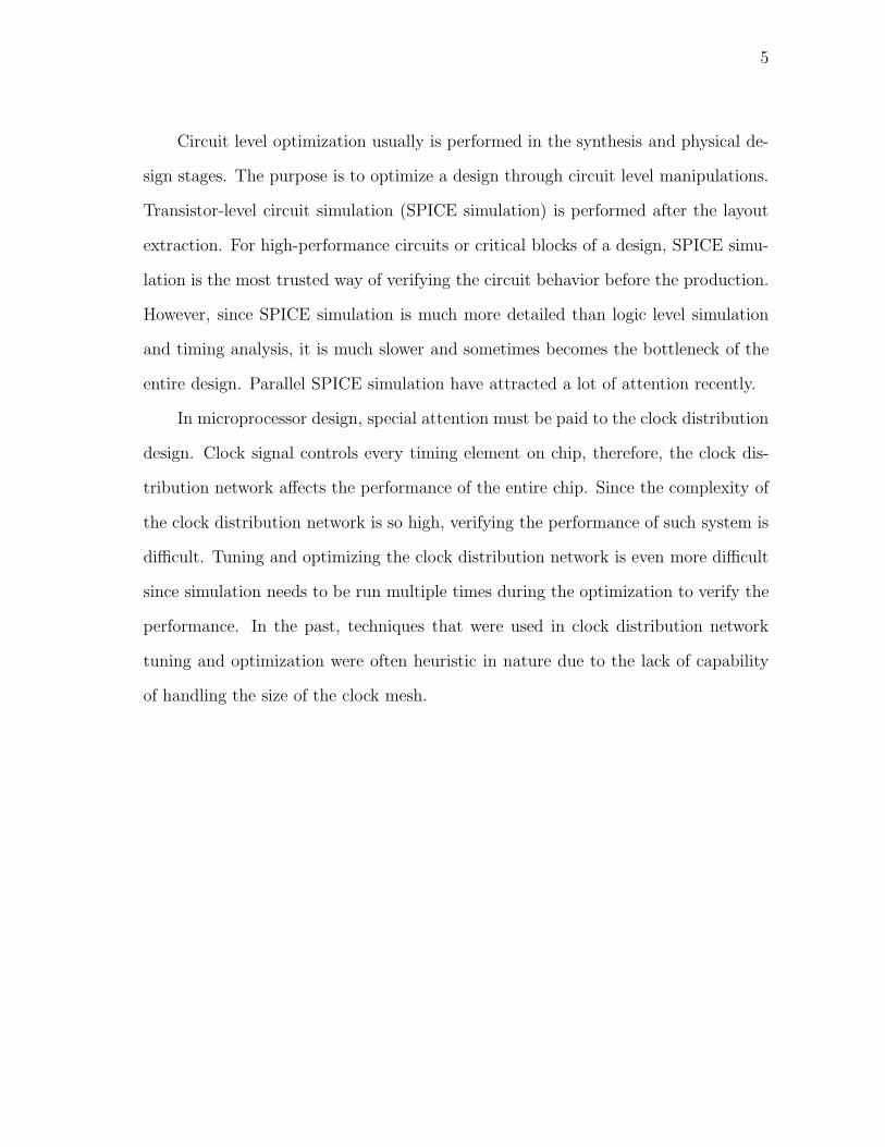
Circuit level optimization usually is performed in the synthesis and physical de-

sign stages. The purpose is to optimize a design through circuit level manipulations.

Transistor-level circuit simulation (SPICE simulation) is performed after the layout

extraction. For high-performance circuits or critical blocks of a design, SPICE simu-

lation is the most trusted way of verifying the circuit behavior before the production.

However, since SPICE simulation is much more detailed than logic level simulation

and timing analysis, it is much slower and sometimes becomes the bottleneck of the

entire design. Parallel SPICE simulation have attracted a lot of attention recently.

In microprocessor design, special attention must be paid to the clock distribution

design. Clock signal controls every timing element on chip, therefore, the clock dis-

tribution network affects the performance of the entire chip. Since the complexity of

the clock distribution network is so high, verifying the performance of such system is

difficult. Tuning and optimizing the clock distribution network is even more difficult

since simulation needs to be run multiple times during the optimization to verify the

performance. In the past, techniques that were used in clock distribution network

tuning and optimization were often heuristic in nature due to the lack of capability

of handling the size of the clock mesh.

6

CHAPTER II

OVERVIEW

This dissertation mainly addresses two CAD applications: 1, parallel analysis and

optimization of mesh based clock distribution network; 2, parallel circuit simulation.

An overview of these two applications and our work are presented in this chapter.

A. Clock Mesh Analysis and Optimization

Mesh based clock distribution network (also known as clock mesh) are used in high

performance microprocessor designs [8, 9, 10] as a way of distributing clock signals to

the entire chip. Due to the inherent wire redundancy introduced by the mesh struc-

ture, clock meshes have excellent performance (e.g. low clock skews) and immunity

to PVT (process-voltage-temperature) variations. However, the sheer complexity of

these clock networks, contributed by the large mesh structure and its tightly coupled

interactions with a large number of clock drivers, presents a daunting circuit analysis

problem. A typical topology of mesh-based clock distribution networks is shown in

Fig. 2 [8, 9]. The top-level clock distribution is routed through a tree and this tree

drives a large mesh spanning the whole chip. The mesh is driven by a large number

of mesh drivers at the leaves of the tree and distributes clock inputs to many bottom-

level clock drivers or flip-flops. An accurate mesh circuit model (e.g. considering

full inductive coupling with power/ground network) may consist of millions of circuit

unknowns and the mesh is tightly coupled with a large number of, say, a few hundred,

nonlinear mesh drivers. Simulating such circuit model alone could take up to hours

of runtime. Tuning/optimizing such network at a desirable accuracy level requires

even longer time since multiple simulations are needed during the optimization.

The ability to efficiently analyze and optimize clock mesh is critical to the design

7

Clock sinks/FFs

Clock drivers… … … …

Fig. 2. Clock distribution using mesh structures.

8

of clock distribution in microprocessors and the performance of the entire chip. SPICE

simulation is intractable for clock mesh analysis due to the problem size. Standard

model order reduction (MOR) algorithms [11, 12, 13, 14], which are powerful for

many large interconnect problems, are only applicable to systems with a limited

number of I/O ports. For clock mesh which could have a few hundred nonlinear

drivers/ports, standard model order reduction algorithms are not the viable solution.

In [15], a sliding window based approach which exploits the locality in the clock

mesh is proposed for fast clock mesh analysis, however, it lacks a systematic way of

controlling the error introduced by the approximation.

In our work, we propose a combination of a highly customized model order reduc-

tion technique called harmonic-weighted model order reduction and a locality based

technique called port sliding to analyze the clock mesh. Our harmonic-weighted model

order reduction technique gains its improved efficiency by analyzing and emphasizing

the harmonic frequency components which are important to the clock mesh perfor-

mance. The second technique, port sliding, exploits the strong locality of the mesh

structure at the output of each mesh clock driver. This technique allows us to com-

pute the clock waveform at the output of each clock driver individually. Therefore,

parallel computing can be naturally applied. In the subsequent step, clock waveforms

at the output of all clock drivers are propagated to clock sinks via fast frequency do-

main post-processing. The combination of harmonic-weighted model order reduction

algorithm and port-sliding technique offers a viable solution for clock mesh analysis.

The per-port based computation in the port sliding technique also allows us to use

parallel computing to expedite the process.

Besides clock mesh analysis, designers also need to perform clock mesh opti-

mization in order to achieve low clock skew. Tuning/optimizing of clock mesh at

a desirable accuracy level requires even more effort since multiple simulations are

9

needed during the optimization. Our fast clock mesh analysis techniques allow us to

perform simulation based clock mesh optimization within a reasonable time frame.

Compared to many other applications in physical design, clock mesh optimization has

been studied to a much less extend. In [8], a divide-and-conquer approach is employed

to tune the wire size in the clock mesh. First, the grid is cut into smaller indepen-

dent linear networks. Each smaller linear network is then optimized in parallel. To

compensate for the loss of accuracy induced by cutting the grid, capacitive loads are

smoothed/spreaded out on the grid. Although the efficiency of the optimization can

be improved by this approach, there is no systematic way of controlling the error.

In [16], very fast combinatorial techniques are proposed for clock driver placement.

These techniques are heuristics in nature. As an alternative to wire sizing and clock

driver placement, clock driver sizing can also be used in clock mesh optimization. For

non-uniform clock load distributions in the clock mesh, if changing the clock driver

placement is impossible due to blockage or other constraints, changing the sizes of

clock drivers can achieve the same or even better results. In our work, we focus on

clock driver sizing.

Since we need to size a large set of clock drivers that are coupled through a large

mesh network, the choice of optimization method is critical. Similar to many prac-

tical problems, the objective function value of the clock mesh optimization problem

is obtained through expensive simulation. Moreover, there is no explicit derivative

information. Standard continuous optimization methods such as sequential quadratic

programming method have many disadvantages in solving this optimization problem.

Due to the lack of explicit derivative information, continuous optimization methods

compute the derivative internally by using inefficient numerical differentiation. Fur-

thermore, these methods usually have small incremental step sizes which make the

progress slow. On the other hand, simulated annealing converges to good final so-

10

lution given sufficiently long time. And it has been parallelized for CAD problems

before [17]. However, the runtime required by simulated annealing to reach a good

final solution is often considered to be extreme long, thus impractical.

In our work, we propose to use the recent asynchronous parallel pattern search

(APPS) method [18, 19] for the clock driver sizing problem. The APPS method has

many advantages over the aforementioned optimization methods in solving the spe-

cific clock mesh optimization problem. First of all, APPS is fully parallelizable. In

the past, the excessive runtime of search based optimization methods often prevents

them from being used as the primary optimization method. In APPS, objective func-

tion value of multiple search points can be evaluated simultaneously. Since majority

of the runtime is spent on objective function value evaluation, running APPS in par-

allel mode gives close to linear speedup over the serial mode. This linear speedup

in runtime as a result of the parallel computing capability makes APPS attractable.

Second, no derivative information is needed in APPS. It is noteworthy that as a

search-based method, APPS has an appealing theoretical convergence property. Un-

der certain mild conditions, APPS is guaranteed to converge to a local optima [18, 19]

and hence it is well suited for tuning of clock driver sizes. Compared to the clock

driver placement and wire sizing problem, the number of variables and solution space

of the clock driver sizing problem are much smaller. This characteristic of the clock

driver sizing problem makes a search based optimization problem such as APPS very

applicable. Although the original APPS method is significantly more efficient com-

pared to other alternative optimization methods, we propose two domain-specific

enhancements: quick estimation and additional search directions to further improve

its speed. Our experimental results show that our domain-specific enhancements can

achieve more than 2x speedup over the original APPS method for a set of clock

meshes.

11

B. Parallel Circuit Simulation

The second application addressed in this dissertation is one of the most used yet

expensive CAD applications: transistor-level time domain circuit simulation. Cir-

cuit simulation is a pre-manufacturing design verification step where circuit behavior

and responses are computed/analyzed by supplying certain inputs to the circuit and

solving the corresponding system equations. Transistor-level time domain circuit sim-

ulation (transient simulation) involves computing the circuit responses as a function

of time.

Due to the ever-increasing complexity of modern VLSI circuits, detailed MOS-

FET models that are required to model the advanced process technology, high accu-

racy requirement for the results and demanding time-to-market requirement in the

semiconductor industry, circuit simulators are hard to keep up with the demands and

often viewed as the bottleneck in the entire design process. There is a persistent

need for better algorithms and techniques which can expedite the circuit simulation

without sacrificing the accuracy.

With the newly introduced parallel multi-core processors [3, 4, 5, 6], the inter-

ests toward parallel circuit simulation is renewed. Parallel circuit simulation is not

a completely new topic. Prior work [20, 21, 22] attempted to realize parallel cir-

cuit simulation from a variety of angles. A practical way to parallelize a SPICE-like

circuit simulator is to parallelize the device evaluation and matrix solve. However,

it has been shown in [23, 24] that the runtime of parallel matrix solvers does not

scale well with the number of processors. Although parallel device evaluation can

reduce the time spent on device evaluation, it introduces additional overhead related

to thread creation, termination, synchronization and merging etc. Therefore, if only

parallel matrix solve and parallel device evaluation are employed in a circuit simula-

12

tor, runtime speedup may stagnate once the number of processors reaches a certain

point. Multilevel Newton algorithm [21] and waveform relaxation algorithm [22] are

a different type of simulation algorithm that based on circuit decomposition. As a

result of circuit decomposition, some subcircuits can be naturally solved in parallel.

Decomposition based circuit simulation algorithms are guaranteed to converge under

certain conditions of the circuit. In practice, many convergence-aiding methods have

to be applied in order to enhance their convergence properties. Recently, a so-called

waveform pipelining approach is proposed to exploit parallel computing for transient

simulation on multi-core platforms [25]. One key observation of the existing parallel

circuit simulation approaches is that most of them can be viewed as Intra-algorithm

Parallelism, meaning that parallel computing is only applied to expedite intermediate

computational steps within a single algorithm. This type of fine grained parallel al-

gorithms often require significant amount of effort on the data and logic dependency

analysis, data and task decomposition, task scheduling and parallel programming

implementation.

In our work, we approach the problem from a completely orthogonal angle. We

exploit Inter-algorithm Parallelism as well as Intra-algorithm Parallelism. The Inter-

algorithm parallelism approach opens up new opportunities for us to explore advan-

tages that are simply not possible when working within one fixed algorithm.

In our Hierarchical Multi-Algorithm Parallel Simulation (HMAPS ) approach,

multiple different simulation algorithms are initiated in parallel using multi-threading

for a single simulation task. These algorithms are synchronized on-the-fly during

the simulation. Different simulation algorithms under the HMAPS framework have

diverse runtime vs. robustness tradeoff. The unique synchronization mechanism in

HMAPS allows us to pick the best performing algorithm at every time point. In

HMAPS, we include the standard SPICE-like algorithm as a solid backup solution

13

which guarantees that the worst case performance of HMAPS is not worse than a

standard serial SPICE simulation. We also include some aggressive and possibly non-

robust simulation algorithms which would normally not be considered in the typical

single-algorithm circuit simulator. In the end, this combination of algorithms in

HMAPS leads to favorable, sometimes, even superlinear speedup in practical cases.

Since the basic multi-algorithm framework is largely independent of other paral-

lelization techniques, we also uses more conventional approaches such as parallel de-

vice model evaluations and parallel matrix solvers to further reduce the runtime. This

combination of high-level multi-algorithm parallelism and low-level intra-algorithm

parallelism forms the unique HMAPS framework which achieves significant runtime

speedup as well as superior robustness in practice.

It is worth noting that our HMAPS approach is not a competitor to the intra-

algorithm parallel simulation approaches, rather, it is an exploration from a orthog-

onal angle which opens up new opportunities for further performance improvement.

HMAPS provides a high-level framework which most of the intra-algorithm paral-

lel simulation methods can be part of. Since the architecture of HMAPS is high-

modularized, simulation algorithms are just separate modules in HMAPS and can

be swapped into and out of HMAPS easily. Such unique architectural feature makes

the initial implementation of HMAPS as well as the possible upgrade of simulation

algorithms easy. A potential limiting factor of HMAPS is the memory usage. Since

HMAPS uses multiple simulation algorithms to solve the same circuit and each algo-

rithm has its own internal data structure, the memory usage of HMAPS is higher than

a single algorithm simulation. On the multi-core platform where all cores/threads

share the memory on a single machine, memory could become a limiting factor for

large circuits. To eliminate this memory limitation, we can migrate HMAPS onto a

distributed computing platform where each simulation algorithm is running on one

14

local machine and communication is through the network.

The combination of inter- and intra-algorithm parallelism in HMAPS creates

complex performance tradeoffs and leads to a very large configuration space. An

HMAPS configuration corresponds to selecting a subset of simulation algorithms from

an algorithm pool and allocating different amount of processing resource (e.g. number

of cores/threads) for each chosen algorithm. If each algorithm in HMAPS can use up

to 4 cores, there could be hundreds of configurations for HMAPS. Since algorithms

have different stepsizes, convergence properties, etc and some algorithms may use

cores more efficiently than others, the runtime of different HMAPS configurations

are vastly different. In our experiments, we have observed that a good configuration

can be 9x faster than a configuration with bad combination of algorithms and core

assignment. Without the performance modeling of HMAPS, it is very difficult to

select the fastest configuration for a simulation.

We propose a parallel performance modeling approach for HMAPS on a given

hardware platform with the primary goal of runtime performance optimization. To

predict the performance of an arbitrary configuration, we propose a systematic com-

posable approach where common computational entities (e.g. matrix solving, nonlin-

ear iteration, device model evaluation and numerical integration etc.) across all sim-

ulation algorithms are independently characterized. These models can then be pieced

together by using a statistical model to predict the performance of any HMAPS con-

figuration. Later, on-the-fly runtime information are combined with the static pre-run

performance models to form dynamic performance models which enable the dynamic

runtime optimization of HMAPS.

15

C. Summary

The techniques and algorithms we developed for these two applications are guided

by the common philosophy that we want to use parallel computing as a leverage to

provide better solutions to difficult CAD problems. If used wisely, parallel computing

can really bring benefits that would be impossible to achieve for sequential approaches.

In our work, parallel computing is used in different ways. In the clock mesh

analysis work, due to the per-port and per-sink nature of the computation, parallel

computing can be naturally applied to speedup the runtime. In modified APPS

for clock mesh optimization, again, due to the independent nature of the objective

function value evaluation process for different search points, parallel computing is

easily applied.

In parallel circuit simulation, there is no easy way of directly applying parallel

computing as we did for clock mesh analysis and optimization. Since the performance

of existing parallel circuit simulation approaches are really confined by the common

limitations and overhead of parallel computing, we develop HMAPS from ground

up with the ideas of truly utilizing the parallel computing powers and avoiding the

constraints faced by the existing fine-grained methods in mind at the very beginning.

As a result, HMAPS really brings some new aspects to the way people think of parallel

circuit simulation. And it achieves great results in practice.

The performance modeling and optimization of HMAPS provides an systematic

way of modeling the performance of parallel programs and tuning the performance of

parallel programs using the performance models.

The relationship between different pieces of research work in this dissertation

are shown in Fig. 3. Clock mesh analysis and modified APPS method for clock

mesh optimization are developed for the clock mesh application. Modified APPS for

16

Parallel VLSI Circuit

Analysis and Optimization

Parallel Circuit Analysis Parallel Circuit

Optimization

Chapter 3

Clock Mesh Analysis

Chapter 3 HMAPS:

Hierarchical Multi-Algorithm

Parallel Simulation

Chapter 5

Performance Modeling and

Optimization of HMAPS

Chapter 4

Modified APPS for

Clock Mesh

Optimization

Fig. 3. Connections between different pieces of research work in this dissertation.

clock mesh optimization uses the clock mesh analysis techniques developed earlier.

HMAPS, performance modeling and runtime optimization of HMAPS are developed

for the parallel circuit simulation application.

This dissertation is organized as follows: Chapter I talks about the background

information of the dissertation. Chapter II discusses the two CAD applications that

will be addressed in the dissertation and provides an overview of our research work.

Chapter III talks about our clock mesh analysis techniques and HMAPS. Chapter IV

discusses a modified Asynchronous Parallel Pattern Search (APPS) method [18, 19]

for the clock mesh optimization problem. Chapter V discusses the parallel program

performance modeling and optimization of HMAPS. Chapter VI concludes this dis-

sertation.

17

CHAPTER III

CIRCUIT ANALYSIS TECHNIQUES

This chapter is organized as follows: in subsection A, analysis techniques for clock

mesh are proposed. The clock mesh analysis techniques proposed in subsection A are

parallel in nature due to the per-port, per-sink computational procedures and will

be used in Chapter IV for parallel clock mesh optimization. In subsection B, a hier-

archical multi-algorithm parallel simulation (HMAPS) approach for general purpose

parallel circuit simulation is proposed.

A. Analysis of Clock Mesh

Clock meshes posses inherent low clock skews and excellent immunity to PVT (pro-

cess, voltage, temperature) variations, and have increasingly found their way to high-

performance IC designs. However, analysis of such massively coupled networks is

significantly hindered by the sheer size of the network and tight coupling between

non-tree interconnects and large numbers of clock drivers. While SPICE simulation

of large clock meshes is completely intractable, standard interconnect model order re-

duction (MOR) algorithms also fail due to the large number of I/O ports introduced

by clock drivers. The presented approach [26] is motivated by the key observation

of the steady-state operation of the clock networks while its efficiency is facilitated

by exploring new clock-mesh specific Harmonic-weighted model order reduction al-

gorithms and locality analysis via port sliding. The scalability of the analysis is

significantly improved by eliminating the need for computing infeasible multi-port

passive reduced order interconnect models with large port count and decomposing

the overall task into very tractable and naturally parallelizable model generation and

FFT/Inverse-FFT (fast fourier transform) operations, all on a per driver or per sink

18

basis. The per-driver and per-sink nature of the approach allows it to executed in

parallel. We demonstrate the application of our approach by feasibly analyzing large

clock meshes with excellent accuracy. Our clock mesh analysis approach will later be

used in Chapter IV for parallel clock mesh optimization.

1. Overview of the Approach

SPICE simulation is very difficult to be applied to clock mesh analysis due to the

excessive long runtime required to solve such massively coupled network. Standard

model order reduction (MOR) algorithms [11, 12, 13, 14], which are powerful for many

large interconnect problems, are only applicable to systems with a limited number of

I/O ports. In the past, the difficulty in analyzing massive networks such as non-tree

clocks and power grids has been recognized and interesting ideas have been proposed

in many ongoing work. Attempts have been made to address this challenge from a

point view of interconnect modeling. New model order reduction algorithms have

been proposed to cope with MOR scalability with respect to the number of ports

[27, 28, 29, 30, 31, 32, 33]. For instance, in [31, 32, 33], techniques have been proposed

to reduce the complexity of model order reduction via means of port compaction

and merging. From a simulation perspective, spacial locality of power grid analysis

has been observed in [34] and a sliding window approach is proposed to analyze

clock meshes via divide-and-conquer in [15]. Here, we shall emphasize that although

power grids and clock meshes share the same feature of high input/output count, the

accuracy requirement of clock network analysis is much more stringent. Despite these

on-going developments, accurate and scalable large clock mesh analysis remains as a

challenge.

One key observation behind our approach is that despite the fact that clock sink

waveforms are often looked at in time domain to evaluate the performances such as

19

Mesh…

Time-domain periodic signal

T0=1/f0

Frequency-domain harmonics0f0

2f0 3f0 …

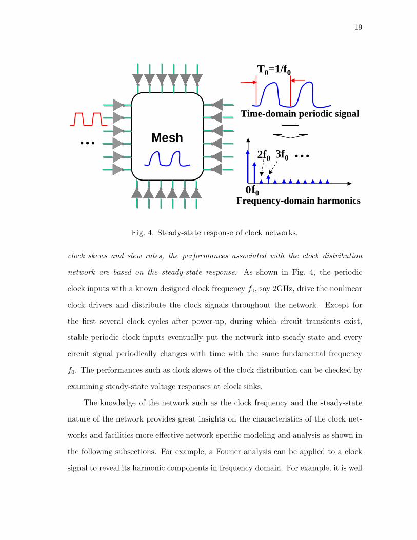
Fig. 4. Steady-state response of clock networks.

clock skews and slew rates, the performances associated with the clock distribution

network are based on the steady-state response. As shown in Fig. 4, the periodic

clock inputs with a known designed clock frequency f0, say 2GHz, drive the nonlinear

clock drivers and distribute the clock signals throughout the network. Except for

the first several clock cycles after power-up, during which circuit transients exist,

stable periodic clock inputs eventually put the network into steady-state and every

circuit signal periodically changes with time with the same fundamental frequency

f0. The performances such as clock skews of the clock distribution can be checked by

examining steady-state voltage responses at clock sinks.

The knowledge of the network such as the clock frequency and the steady-state

nature of the network provides great insights on the characteristics of the clock net-

works and facilities more effective network-specific modeling and analysis as shown in

the following subsections. For example, a Fourier analysis can be applied to a clock

signal to reveal its harmonic components in frequency domain. For example, it is well

20

known that a complete symmetric clock signal with 50% duty cycle does not exhibit

any even order harmonics. However, such network-specific knowledge has not been

exploited in prior work.

The insights on clock network operation allow us to develop a clock-network spe-

cific model order reduction algorithm where only signal transfers at discrete harmonic

frequencies with known fundamental clock frequency are preserved. Moving one step

further, a harmonic-weighted scheme is proposed to weight the harmonics that are

important to the time domain performance measures, such as clock skews and slew

rates, more significantly during projection-based model order reduction.

The second proposed technique, port sliding, exploits the locality of the mesh

structure in a spirit similar to [15]. However, this new port sliding scheme exploits a

much stronger locality observed right at the output of each mesh clock drive. Each

driving point waveform is computed individually with fine accuracy control while

the complexity introduced by the large number of faraway drivers is systematically

tackled using driver merging, and a combination of the harmonic-weighted model

order reduction and another new weighted model order reduction technique that is

based on the importance of faraway drivers on the driving point. The same steady-

state observation allows us to efficiently propagate all driving point waveforms to

the interested clock sinks via frequency-domain post-processing using efficient FFT

and IFFT (inverse FFT) operations. Our approach provides a systematic divide-and-

conquer methodology for large mesh analysis, wherein the overall task is broken down

into easily trackable small pieces, which can be further processed in parallel.

21

2. Harmonic-Weighted Model Order Reduction

An multi-input multi-output (MIMO) passive interconnect network can be described

using the following circuit equations

Cd

dt+Gx = Bu, y = LTx, (3.1)

where G,C ∈ Rn×n describe the resistive and energy storage elements in the circuit,

u ∈ Rm is the input vector, x ∈ Rn is the vector of unknown voltages and currents,

and B,L ∈ Rn×m are the input and output matrices, respectively.

The widely used passive model reduction algorithm PRIMA [14] generates a

reduced order model of (3.12) by computing an orthonormal basis V of the Krylov

subspace spanned by colspanR,AR,A2R, · · · , where A ≡ −G−1C and R ≡ G−1B,

and AiR is the i-th order block transfer function moment. The reduced order model

is given by a set of system matrices of a smaller dimension

G = V TGV, C = V TCV, B = V TBL = V TL, (3.2)

where the order of the reduced order model is determined by the column dimension

of V , denoted as q. To see why the standard PRIMA algorithm may fail to produce

a meaningfully sized reduced order model for a passive network with a large number

of I/Os, let us consider a clock mesh with 100 nonlinear clock drivers. Assuming that

20 moments are matched for each driver port in order to accurately match the system

transfer functions, then a reduced order model with a size q = 2, 000 will be computed.

However, the computation and simulation of such large dense 2, 000×2, 000 model are

extremely timing consuming, which may defeat the purpose of model order reduction.

Exploring the network-specific knowledge discussed in subsection 1, one would argue

that the reduced order model produced by PRIMA is generic in the sense that it

22

well matches the frequency responses of the network over a continuous frequency

range regardless the operation of the network. However, this is not needed for clock

meshes, where only a discrete set of harmonic frequency components with a known

fundamental frequency f0 are important.

This naturally leads to the use of a multi-point expansion based model order

reduction where the transfer functions (or zero-th order moments) at each harmonic

(corresponding to the expansion point s = j2πkf0) are computed and included into

the projection matrix V to facilitate projection-based model order reduction. It can

be shown that the resulting model will match the system transfer functions at all

these harmonic frequencies considered [35]. To generate a real reduced order model,

each complex transfer function vector needs to be split into the real and imaginary

parts and contributes two projection vectors in V . The use of multi-point projection

along the imaginary axis allows us to focus on useful frequency components relevant

to the operation of the clock mesh, however, it does not provide an immediate benefit

for controlling model complexity. To see this, let us go back to the previous example.

Now, assume that we need to match the frequency responses at DC and 10 other

harmonics. Since each complex transfer function vector contributes two projection

vectors, the final size of the 100-input reduced order model is 2, 100, providing a

similarly large sized model.

In the proposed harmonic-weighted model reduction algorithm, we move one

important step further: we not only look at the set of discrete harmonic frequencies

but also the importance of each harmonic component on the network performance

(e.g. clock skews) to guide model order reduction.

Without loss of generality, let us consider an arbitrary periodic clock signal,

possibly observed at one clock sink, in Fig. 5. The goal of the following analysis is to

find out the harmonic components that are critical to time-domain clock distribution

23

t

Vdd

0.5Vdd

0.8 Vdd

0.2 Vdd

T50%

Fig. 5. Voltage-crossing times of a clock signal.

performances (e.g. clock skew) and use this result to guide model order reduction.

If we target at of one of the most important performances, clock skew, then it is

instrumental to find out the sensitivities of the 50%Vdd crossing time, T50%, w.r.t. to

the variations of each harmonic component’s magnitude and phase. To do this, we

start from the Fourier series expansion of the clock signal

f(t) =∞

∑

k=−∞

Akejkω0t, (3.3)

where ω0 = 2πf0 and Ak is the Fourier coefficient at the frequency component kω0.

At t = t50%, we know that the clock signal crosses 0.5Vdd

f(T50%) =

∞∑

k=−∞

Akejkω0T50% = Vdd/2. (3.4)

Now use a phasor representation for each complex Fourier coefficient Ak = |Ak|ejφk

and (3.4) is rewritten as

f(T50%) =

∞∑

k=−∞

|Ak|ej(kω0T50%+φk) = Vdd/2. (3.5)

Next, the sensitivities of T50% with respect to the k-th harmonic component are

derived. Since the conjugate relationship |Ak| = |A−k| and φk = −φk must be

24

enforced for real time domain signals, the terms that are contributed by k-th and −k-

th harmonics in (3.5) are combined to generate 2|Ak|cos(kω0T50%+φk). Differentiating

both sides of the equation w.r.t |Ak| gives

2 cos(kω0T50% + φk)− 2|Ak|kω0 sin(kω0T50% + φk)∂T50%

∂|Ak|

∂T50%

∂|Ak|jω0

∞∑

n=−∞,n 6=±k

n|An|ejnω0T50%+φn = 0.

(3.6)

Finally, we get

∂T50%

∂|Ak|=

2 cos(kω0T50% + φk)

2kω0|Ak| sin(kω0T50% + φk)

−jω0

∑∞

n=−∞,n 6=±k n|An|ejnω0T50%+φn

(3.7)

Similarly the sensitivity w.r.t φk is

∂T50%

∂φk

=2|Ak| sin(kω0T50% + φk)

−2kω0|Ak| sin(kω0T50% + φk)

+jω0

∑∞n=−∞,n 6=±k n|An|e

jnω0T50%+φn

(3.8)

To consider the magnitude difference across all the harmonics, we modify (3.7)

to evaluate the sensitivity of T50% with respect to the relative change in|Ak|

∂T50%

∂|Ak|=∂T50%

∂|Ak||Ak|. (3.9)

To generate a single weight Wk for the k-th harmonic to guide the model order

reduction, (3.7) and (3.9) are normalized between 0 and 1.0, respectively and added

up

Wk =∂T50%

∂|Ak| nom

+∂T50%

∂φk nom

. (3.10)

Since clock delays and skews are obtained by checking the 50%Vdd crossing times of

25

0 0.5 1

x 10−9

0

0.5

1

Clock Signal

0 5 10 15 200

0.5

1Magnitude of Harmonics

0 5 10 15 200

0.2

0.4

0.6

0.8

1Partial Weights

MagPhase

0 5 10 15 200

0.5

1Final Weights

Fig. 6. Harmonic weighting for a clock signal.

clock signals at the sinks, Wk tells us quantitatively how important it is to preserve

the accuracy of the signal transfer at frequency kω0. The sensitivities of other perfor-

mance measures can be handled in a similar fashion. For instance, one can compute

the sensitivities of 20% and 80% Vdd crossing times to extract the sensitivities of the

slew rate with respect to multiple harmonic components.

In Fig. 6, magnitudes of the harmonic components, normalized magnitude and

phase T50% sensitivities (partial weights) and the final weights (W ′ks) are shown for a

clock signal. It is interesting to note that although the DC component has the largest

magnitude, T50% is most sensitive to the first harmonic. One question naturally arises:

The importance of each harmonic, or Wk, can be computed easily for a given clock

26

0 0.5 1

x 10−9

0

0.5

1

Clock Signal

0 5 10 15 200

0.5

1Magnitude of Harmonics

0 5 10 15 200

0.2

0.4

0.6

0.8

1Partial Weights

MagPhase

0 5 10 15 200

0.5

1Final Weights

Fig. 7. Harmonic weighting for a clock signal with overshoot.

signal as described before. But how to obtain these weights during the model order

reduction phase where the circuit response of the clock network is not known yet?

In practice, this problem can be addressed by noting that W ′ks are rather constant

across typical clock signal waveforms. To see this, the weights are re-computed for

another clock signal with overshoot in Fig. 7. As can be seen, the new W ′ks are rather

consistent with the previous ones. Therefore, W ′ks can be pre-computed based on

a typical clock waveform, and incorporated in the harmonic-weighted model order

reduction algorithm described as follows.

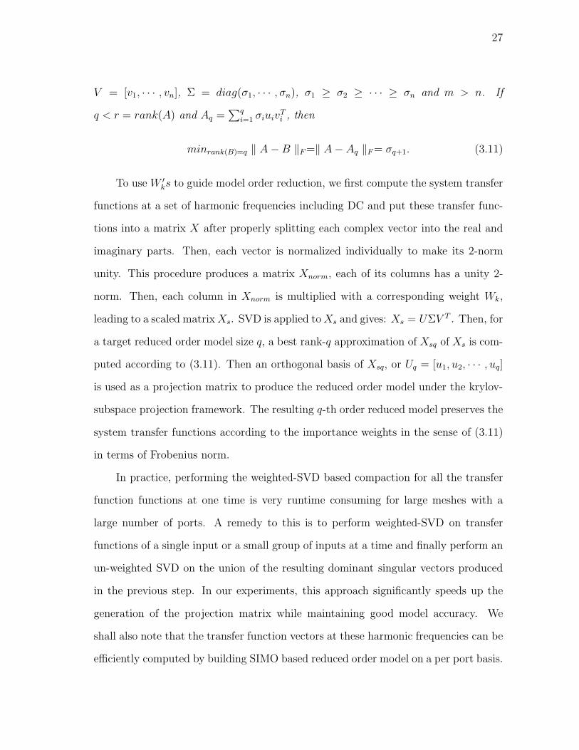
Note the well-known result on SVD [36]:

Theorem 1 Let A = UΣV T ∈ Rm×n be the SVD of A, where U = [u1, · · · , un],

27

V = [v1, · · · , vn], Σ = diag(σ1, · · · , σn), σ1 ≥ σ2 ≥ · · · ≥ σn and m > n. If

q < r = rank(A) and Aq =∑q

i=1 σiuivTi , then

minrank(B)=q ‖ A−B ‖F =‖ A− Aq ‖F= σq+1. (3.11)

To use W ′ks to guide model order reduction, we first compute the system transfer

functions at a set of harmonic frequencies including DC and put these transfer func-

tions into a matrix X after properly splitting each complex vector into the real and

imaginary parts. Then, each vector is normalized individually to make its 2-norm

unity. This procedure produces a matrix Xnorm, each of its columns has a unity 2-

norm. Then, each column in Xnorm is multiplied with a corresponding weight Wk,

leading to a scaled matrixXs. SVD is applied toXs and gives: Xs = UΣV T . Then, for

a target reduced order model size q, a best rank-q approximation of Xsq of Xs is com-

puted according to (3.11). Then an orthogonal basis of Xsq, or Uq = [u1, u2, · · · , uq]

is used as a projection matrix to produce the reduced order model under the krylov-

subspace projection framework. The resulting q-th order reduced model preserves the

system transfer functions according to the importance weights in the sense of (3.11)

in terms of Frobenius norm.

In practice, performing the weighted-SVD based compaction for all the transfer

function functions at one time is very runtime consuming for large meshes with a

large number of ports. A remedy to this is to perform weighted-SVD on transfer

functions of a single input or a small group of inputs at a time and finally perform an

un-weighted SVD on the union of the resulting dominant singular vectors produced

in the previous step. In our experiments, this approach significantly speeds up the

generation of the projection matrix while maintaining good model accuracy. We

shall also note that the transfer function vectors at these harmonic frequencies can be

efficiently computed by building SIMO based reduced order model on a per port basis.

28

Such choice only requires one LU factorization of the system conductance matrix G.

The complete algorithm flow is shown in Algorithm 1.

Algorithm 1 Harmonic-Weighted Model Order ReductionIn: Full model: G, C, B, L; f0, Ctrl fac: κ, Red-mod. size: SR

Out: Reduced order model:G, C, B, L .

1: Compute W ′ks using (3.6), (3.7), (3.8) and (3.9).

2: V ← [ ].3: for each input i do

4: Compute the transfer function at dc: Vi ← TF (0, i)5: for each harmonic k, k = 1, · · · ,Nh do

6: Compute the transfer function: TF(k, i).7: Vi ← [Vi, ReTF (k, i), ImTF (k, i)].8: end for

9: Normalize each column in Vi and multiply each column using the corresponding weightWk.

10: Perform SVD on the weighted Vi matrix: Vi,w = Pi

∑

i QTi .

11: Keep the first κ dominant singular vectors in Pi:V ← [V [pi,1, · · · , pi,κ]].

12: end for

13: Perform SVD on V : V = P∑

QT .14: Keep the first SR dominant singular vectors X of P , X = [p1, · · · , pSR

] for modelreduction:G = XT GX, C = XT CX, B = XT B, L = XT L

3. Port Sliding

To further increase the scalability of large clock mesh analysis, in this subsection we

present a port sliding scheme, which provides fast and efficient driving point waveform

computation at the output of each mesh clock driver as illustrated in Fig. 8. This

approach is based on the understanding that computing a compact and accurate

multi-port passive model for the complete mesh is rather challenging when the number

of ports is high. Hence, it is rather desired to facilitate efficient large mesh analysis

via localized computation.

29

Our localized analysis is based upon computing each driving point waveform

individually. Although our port sliding scheme looks similar to the sliding window

technique in [15], these two approaches are significantly different. In [15], a large

mesh is heuristically divided into smaller partitions and then each partition is solved

by completely neglecting circuit elements out side of the partition. The network

partitioning is critical for controlling the accuracy, however, it is done completely

based on heuristics.

Differently, our approach exploits a very strong locality effect in the network.

That is, the driving point voltage waveform is predominately determined by the

corresponding driver and its neighboring drivers, the influence of other drivers drop

off very quickly. In contrast, an internal mesh node that is not directly driven by

any driver may be influenced significantly by a large number of drivers. Another

important feature of our approach is that during each driving point computation, all

circuit elements including the mesh and all drivers are considered while the overall

analysis complexity is controlled by three possible methods as described as follows.

The first method is called driver merging. The strong locality allows us to reduce

the complexity of driving point waveform analysis by significantly approximating the

effects of faraway drivers. As shown in Fig. 9, the drivers that are far away from the

driving point are merged into a single ”effective” driver with an average size among

these merged drivers. This effective driver touches the mesh around the geometrical

center of driving points of the merger drivers and its input also represents an average

among the inputs of the merged drivers. The nearby drivers are retained to safeguard

the analysis accuracy. After driver merging, the effective number of I/O ports of the

mesh is significantly reduced, a reduced order model can be easily produced using

a standard algorithm like PRIMA. This reduced mesh model is simulated together

with all clock drivers. After this simulation, only the voltage response at the current

30

?

Fig. 8. Efficient driving point waveform computation using port sliding.

driving point is retained and responses at other ports of the network are neglected.

Then, the next driving point is selected and the whole process repeats until all the

driving point voltage waveforms are computed.

The second method is called importance-weighted model order reduction. As

an alterative approach to driver merging, signal transfers associated with faraway

ports are coarsely preserved for the purpose of driving point computation. As shown

in Fig. 10, a model order reduction procedure similar to what is in subsection 2 is

adopted. First, the harmonic-weighted scheme presented in subsection 2 is applied

to compress transfer functions associated with faraway ports. As described before,

this compression is guided by importance of different harmonic components. Further

compression can be achieved by computing another set of importance weights, but

in terms of the influence of each far away driver on the driving point that is being

31

?

Merged driver

ROM

for

Fig. 9. Merging of faraway drivers.

examined. This new importance can be rather efficiently obtained by computing the

DC and first order moments of the transfer function relating the faraway port to

the driving point. After the projection matrix is compressed by the combination of

two weighting scheme, a multi-port reduced order model is computed and simulated

with all nonlinear drivers to obtained the desired driving point voltage waveform.

In comparison to driver merging, the complexity of this approach is higher due to

the larger number of ports considered and the computational cost of the SVD-based

compaction. However, the advantage is that all the mesh drivers/ports are considered,

systematically, through the venue of systematic model order reduction.

The two previous approaches can be combined naturally to form the third ap-

proach called combined driver merging and MOR which achieves the best tradeoff be-

tween efficiency and robustness. Faraway mesh drivers can be first grouped according

to geometrical closeness. Then, drivers within each group are merged and multiple

faraway ”effective” drivers are resulted. Then, same as in the previous method, a

weighted-MOR approach can be then applied. Here, since the total number of drivers

that are considered in the model order reduction may be significantly reduced by

32

ROM

High-order moment matching/TF for neighboring ports

Use importance guided SVD to compress faraway ports

Fig. 10. Compaction of faraway ports using importance-weighted SVD.

merging, the runtime efficiency can be noticeably improved.

Once all the driving point voltage waveforms are obtained, the clock signal at

each sink can be computed by propagating all the driving point waveforms to the

sink through the passive mesh. As shown in Fig. 11, this procedure can be done on a

per port/sink basis as follows. First, the time-domain driving point voltage waveform

at a particular port is first converted back to frequency domain via FFT. Then the

FFT results can be simply multiplied with the transfer functions relating the port to

the sink so as to obtain the frequency domain contribution of this particular driving

point waveform to the sink node response. Once the frequency domain contributions

from all the ports are computed and summed up, a frequency domain representation,

or Fourier expansion, of the sink node response is obtained. Finally this frequency

domain representation is transformed to time domain using inverse FFT and then

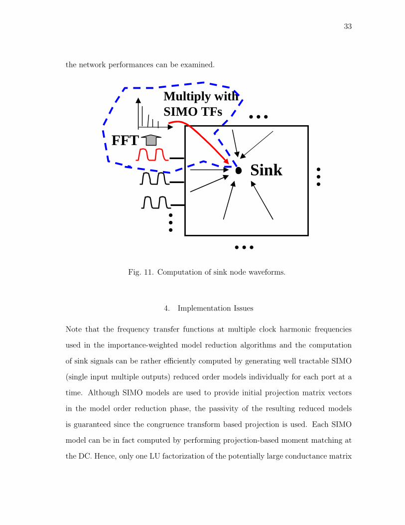
33

the network performances can be examined.

……

……

Sink

FFT

Multiply with SIMO TFs

Fig. 11. Computation of sink node waveforms.

4. Implementation Issues

Note that the frequency transfer functions at multiple clock harmonic frequencies

used in the importance-weighted model reduction algorithms and the computation

of sink signals can be rather efficiently computed by generating well tractable SIMO

(single input multiple outputs) reduced order models individually for each port at a

time. Although SIMO models are used to provide initial projection matrix vectors

in the model order reduction phase, the passivity of the resulting reduced models

is guaranteed since the congruence transform based projection is used. Each SIMO

model can be in fact computed by performing projection-based moment matching at

the DC. Hence, only one LU factorization of the potentially large conductance matrix

34

G is needed. The transfer functions used in the clock sink computation can be pro-

vided by the same set of SIMO models. Again, the passivity of the analysis is not any

issue since each clock sink signal is obtained by summing up contributions from all

ports using FFT/IFFT computations without involving simulation of a reduced order

model with nonlinear drivers. Importantly, the major steps of importance-weighted

model order reduction algorithms and the sliding port scheme can be naturally paral-

lelized. All these computations are on a per port and/or per sink basis. Therefore, the

efficiency of our techniques can be significantly improved through parallel processing.

5. Experimental Results

The efficiency and accuracy of the proposed harmonic-weighted model order reduction

algorithm and the port sliding scheme are demonstrated on a set of clock meshes.

These two schemes are tested on clock meshes with different sizes, different number

of inputs and different driver input skews. We compare our harmonic-weighted model

order reduction algorithm with PRIMA [14]. For the port sliding scheme, we show

the runtime and accuracy of the three different port sliding methods: driver merging,

importance-weighted model reduction, combined driver merging and MOR. We also

make comparison with the sliding window scheme [15]. The proposed algorithms have

been implemented in C++. The experiments were conducted on a PC running Linux

operating system with 4GB memory.

First we consider a mesh with 13k elements including resistors, capacitors and

inductors and 17 ports. All 17 ports are driven by clock buffers. Fig. 12(a) compares

the time domain response at one sink node for PRIMA, harmonic-weighted MOR

and full simulation. The size of the reduced model generated by PRIMA is 34 while

the size of the reduced model generated by harmonic-weighted MOR is 24. Although

harmonic-weighted MOR generates a smaller size reduced order model, it captures

35

Table I. Runtime(s) comparison for full simulation, PRIMA and Harmonic-weighted

MOR

Mesh Size #Drivers Full Simu. PRIMA WeightedGen. Simu. Gen. Simu.

mesh1 13k 17 47.5s 6.86s 30.43s 70.9s 28.41smesh2 27k 53 2h2min 199.4s 12min 49s 22min 5s 428.4s

the time domain response better than PRIMA. Fig. 12(b) zooms in the same plot in

Fig. 12(a). The error for PRIMA is around 6ps while the error for harmonic-weighted

MOR is negligible.

Next, we consider a larger mesh with 27k elements including resistors, capacitors

and inductors and 53 clock buffers. PRIMA generates a reduced order model of

size 159 while Harmonic-weighted MOR generates a reduced order model of size 111,

which is 30% less than the model from PRIMA. Fig. 13(a) and 13(b) show that

with a much smaller size reduced order model, harmonic-weighted MOR can achieve

the same accuracy compared with PRIMA. Table I shows the runtime comparison

between PRIMA, harmonic-weighted MOR and full simulation. For PRIMA and

harmonic-weighted MOR, runtime includes the model generation time and model

simulation time. The model generation time for Harmonic-weighted MOR is usually

longer than PRIMA, which is due to the SVD operations. However, this is one time

cost for passive mesh. The same reduced order model can be reused if the inputs or

sizes of the drivers are changed. It shall also be noted that the simulation time of

the reduced order model produced by harmonic-weighted MOR is less because of the

smaller size reduced order model.

As described before, we combine the harmonic-weighted MOR with port sliding

to provide analysis scalability for large mesh structures. We compare three port

sliding methods proposed in subsection 3: driver merging, importance-weighted MOR,

36

0 0.5 1 1.5 2

x 10−9

−0.2

0

0.2

0.4

0.6

0.8

1

1.2

Time(s)

Vol

tage

(v)

Exact PRIMAWeighted

(a)

1.62 1.64 1.66 1.68 1.7 1.72 1.74

x 10−10

0.495

0.5

0.505

0.51

0.515

Time(s)

Vol

tage

(v)

Full simulation

Weighted

PRIMA

(b)

Fig. 12. (a)Comparison of time domain response between PRIMA and Harmon-

ic-weighted MOR at one sink node of mesh1. (b)Zoomed-in view of Fig. 12(a).

0 5 10 15

x 10−10

0

0.2

0.4

0.6

0.8

1

1.2

Time(s)

Vol

tage

(v)

ExactPRIMA

Weighted

(a)

6.455 6.46 6.465 6.47 6.475 6.48 6.485

x 10−10

0.4995

0.5

0.5005

0.501

0.5015

Time(s)

Vol

tage

(v) Exact

PRIMA

Weighted

(b)

Fig. 13. (a)Comparison of time domain response between PRIMA and Harmon-

ic-weighted MOR at one sink node of mesh2. (b)Zoomed-in view of Fig. 13(a).

37

Table II. Comparison between three port sliding methodsckt Size #Drivers Spice Driver merging Importance.weighted Comb. merge and MOR

runtime ave. err max. err runtime ave. err max. err runtime ave. err max. errmesh2 27K 53 2h2mins 14min30s 2.3ps 4.0ps 32min20s 0.2ps 1.2ps 17min40s 0.4ps 2.2psmesh3 50K 100 3h 22min10s 2.6ps 4.7ps 45min37s 0.3ps 1.3ps 28min52s 0.8ps 2.5psmesh4 100K 100 6h30min 30min36s 2.4ps 4.2ps 1h2min 0.5ps 1.5ps 40min16s 0.6ps 1.9psmesh5 300K 200 NA 2h34min - - - - - 3h10min - -

combined driver merging and MOR. And we also make comparison between our port

sliding schemes and the sliding window scheme [15].

First, we test these three methods on the same mesh with 27k elements and 53

ports. For our port sliding scheme, the accuracy of the driving point waveform com-

putation is critical to the entire mesh analysis. First, we demonstrate the accuracy of

our driving point waveform analysis. Fig. 14(a) shows the comparison for a driving

point waveform obtained from four different methods: full simulation, driver merg-

ing, importance-weighted MOR, combined merging and MOR. Fig. 14(b) shows the

comparison for a sink node waveform obtained from four different methods. Table

II summarizes the runtime and accuracy for these four methods. The importance-

weighted model reduction gives the best accuracy compared with full simulation, and

it also takes the longest time to generate and simulate the model. The combined

driver merging and MOR gives the second best accuracy, and it is more runtime ef-

ficient than the importance-weighted method. Driver merging is the fastest method,

however, at a cost of lower accuracy.

We also compare our approaches with the sliding window scheme using mesh3.

And we use a typical window size as described in [15]. Fig. 15 shows a comparison at

the clock waveform at a sink node where the sliding window scheme has large error.

The example shows the heuristic nature of the accuracy control in the sliding window

scheme due to the non-systematic partitioning. In comparison, our approach provides

38

a very tight accuracy control as at any point time there is no circuit element being

discarded.

Fig. 16 illustrates the runtime breakdown for each operation step of the three

port sliding methods for mesh3. It includes the model generation time, simulation

time and the post-processing FFT/IFFT time. For large size meshes, the model

generation, driving point waveform computation and post-processing FFT/IFFT in

our sliding port scheme can be all fully parallelized to achieve further improvement

on runtime efficiency as our analysis is conducted on a per driver or per sink basis.

As a result, the total runtime of our algorithms can be linearly scaled down as the

number of parallel processing elements (CPUs) increases.

0 0.2 0.4 0.6 0.8 1

x 10−9

−0.2

0

0.2

0.4

0.6

0.8

1

1.2

Time(s)

Vol

tage

(v)

Exact,

Driver merging

Importance−weighted,Combined,

(a)

0 0.2 0.4 0.6 0.8 1

x 10−9

−0.2

0

0.2

0.4

0.6

0.8

1

1.2

Time(s)

Vol

tage

(v)

Exact,Importance−weighted,Combined,

Drivermerging

(b)

Fig. 14. (a)Comparison of driving point waveform between full simulation and three

different port sliding methods for mesh2. (b)Comparison of the time domain

waveform of a clock sink between full simulation and driver merging scheme

for mesh2.

39

0 0.1 0.2 0.3 0.4 0.5 0.6 0.7 0.8 0.9 1

x 10−9

−0.2

0

0.2

0.4

0.6

0.8

1

1.2

Time(s)

Vol

tage

(v)

Sliding window Importance−weighted

Exact

Combined

Fig. 15. Comparison of the time domain waveform of a clock sink between sliding

window scheme and port sliding scheme.

40

Fig. 16. Runtime breakdown for mesh3.

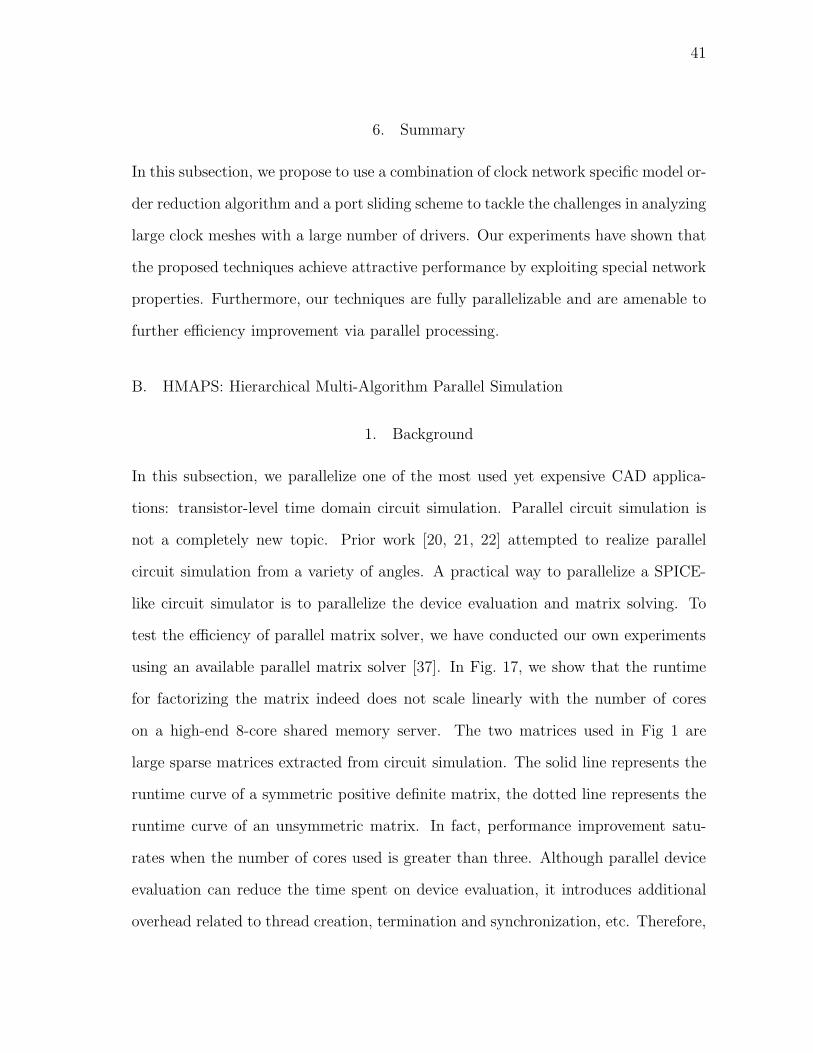
41

6. Summary

In this subsection, we propose to use a combination of clock network specific model or-

der reduction algorithm and a port sliding scheme to tackle the challenges in analyzing

large clock meshes with a large number of drivers. Our experiments have shown that

the proposed techniques achieve attractive performance by exploiting special network

properties. Furthermore, our techniques are fully parallelizable and are amenable to

further efficiency improvement via parallel processing.

B. HMAPS: Hierarchical Multi-Algorithm Parallel Simulation

1. Background

In this subsection, we parallelize one of the most used yet expensive CAD applica-

tions: transistor-level time domain circuit simulation. Parallel circuit simulation is

not a completely new topic. Prior work [20, 21, 22] attempted to realize parallel

circuit simulation from a variety of angles. A practical way to parallelize a SPICE-

like circuit simulator is to parallelize the device evaluation and matrix solving. To

test the efficiency of parallel matrix solver, we have conducted our own experiments

using an available parallel matrix solver [37]. In Fig. 17, we show that the runtime

for factorizing the matrix indeed does not scale linearly with the number of cores

on a high-end 8-core shared memory server. The two matrices used in Fig 1 are

large sparse matrices extracted from circuit simulation. The solid line represents the

runtime curve of a symmetric positive definite matrix, the dotted line represents the

runtime curve of an unsymmetric matrix. In fact, performance improvement satu-

rates when the number of cores used is greater than three. Although parallel device

evaluation can reduce the time spent on device evaluation, it introduces additional

overhead related to thread creation, termination and synchronization, etc. Therefore,

42

if only parallel matrix solving and parallel device evaluation are employed in a cir-

cuit simulator, runtime speedup may stagnate once the number of processors reaches

certain point. Multilevel Newton algorithm [21] and waveform relaxation algorithm

[22] are based on circuit decomposition. As a result of circuit decomposition, some

subcircuits can be naturally solved in parallel. Decomposition based circuit simula-

tion algorithms are guaranteed to converge under certain assumptions of the circuit.

There has been a successful implementation of the variant of the Multi-level Newton-

Raphson method: APLAC [38] which uses convergence aiding methods to enhance

the convergence properties. Note that most prior work targets traditional supercom-

puters and computer clusters, and do not explore the favorable characteristics of the

current multi-core processors such as shared-memory based communication scheme,

reduced inter-processor communication overhead, uniformed computing power among

cores, etc. Recently, a so-called waveform pipelining approach is proposed to exploit

parallel computing for transient simulation on multi-core platforms [25].

One key observation is that most of the existing parallel circuit simulation ap-

proaches can be viewed as Intra-algorithm Parallelism, meaning that parallel com-

puting is only applied to expedite intermediate computational steps within a single

algorithm. This choice often leads to fine grained parallel algorithms which require sig-

nificant amount of data dependency analysis and programming effort. In this work, we

approach the problem from a somewhat unorthodox angle, we explore Inter-algorithm

Parallelism as well as Intra-algorithm Parallelism. This combination of different lev-

els of parallelism not only opens up new opportunities, but also allows us to explore

advantages that are simply not possible when working within one fixed algorithm.

The presented Hierarchical Multi-Algorithm Parallel Simulation (HMAPS ) ap-

proach extends our earlier preliminary work [39, 40] along a similar direction. Mul-

tiple different simulation algorithms are initiated in parallel using multi-threading

43

1 2 3 4 5 6 7 80.2

0.4

0.6

0.8

1

Number of Cores/Threads

Nor

mal

ized

Run

time

SPD Matrix

Unsymmetric Matrix

Fig. 17. Performance evaluation of a parallel matrix solver.

44

for a single simulation task. These algorithms are synchronized on-the-fly during the

simulation. Because they have a diverse CPU-time vs. convergence property tradeoff,

we pick the best performing algorithm at every time point. We include the standard

SPICE-like algorithm as a solid backup solution which guarantees that the worst case

performance of HMAPS is no worse than a serial SPICE simulation. We also include

some aggressive and, possibly non-robust, simulation algorithms which would nor-

mally not be considered in the typical single-algorithm circuit simulator. In the end,

this combination of algorithms in HMAPS leads to favorable, sometimes, even super-

linear speedup in practical cases. In addition to exploiting diversities in algorithms,

the multi-algorithm framework also allows algorithms to share some useful realtime

information of the circuit in order to achieve better runtime performance.

Since the basic multi-algorithm framework is largely independent of other paral-

lelization techniques, we also uses more conventional approaches such as parallel de-

vice model evaluations and parallel matrix solvers to further reduce the runtime. This

combination of high-level multi-algorithm parallelism and low-level intra-algorithm

parallelism forms the hierarchical MAPS approach which not only utilizes the hard-

ware resources better but also achieves better runtime performance than MAPS [40].

2. Overview of the Approach

Before going into the details, we provide some observations of various parallel circuit

simulation approaches.

Fig. 18 illustrates four computation models and their corresponding computing

platforms. The scheme on the top left is a sequential computing model where a

single task/algorithm is running on a single core CPU. Traditional sequential SPICE

simulation falls into this category. The scheme on the top right is a parallel computing

model where one task is divided into smaller subtasks, and each subtask is running

45

single

core

single algorithm

Single algorithm on

single core CPU

core A

Single algorithm on

multi-core CPU

algorithm B

Multi-algorithm on

multi-core CPU

core B core C

core D

core A

core B core C

core D

A

BC

D

algorithm C

algorithm A algorithm D

algorithm Balgorithm C

algorithm A algorithm D

Hierarchical multi-algorithm on

multi-core CPU

Fig. 18. Four different computing models of circuit simulation approaches.

on a core of a multi-core CPU. Intra-algorithm parallel approaches such as parallel

device evaluation, parallel matrix solve fall into this category. The scheme on the

bottom left is another model for parallel computing where multiple algorithms are

being executed for a single simulation task on multiple cores and communication is

allowed between different algorithms. The MAPS approach [39, 40] belongs to this

category. The fourth model is the combination of the second and third model. The

hierarchical MAPS approach proposed in this paper implements this model.

In practice, a single simulation algorithm may behave differently within the entire

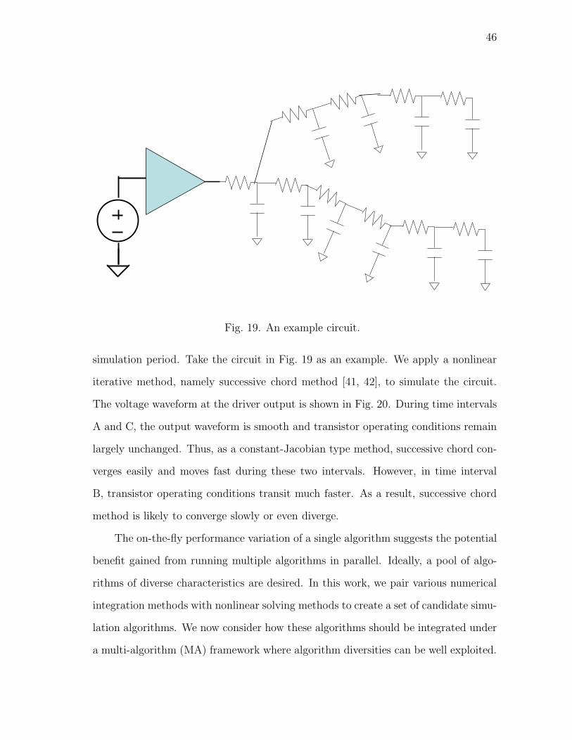
46

Fig. 19. An example circuit.

simulation period. Take the circuit in Fig. 19 as an example. We apply a nonlinear

iterative method, namely successive chord method [41, 42], to simulate the circuit.

The voltage waveform at the driver output is shown in Fig. 20. During time intervals

A and C, the output waveform is smooth and transistor operating conditions remain

largely unchanged. Thus, as a constant-Jacobian type method, successive chord con-

verges easily and moves fast during these two intervals. However, in time interval

B, transistor operating conditions transit much faster. As a result, successive chord

method is likely to converge slowly or even diverge.

The on-the-fly performance variation of a single algorithm suggests the potential

benefit gained from running multiple algorithms in parallel. Ideally, a pool of algo-

rithms of diverse characteristics are desired. In this work, we pair various numerical

integration methods with nonlinear solving methods to create a set of candidate simu-

lation algorithms. We now consider how these algorithms should be integrated under

a multi-algorithm (MA) framework where algorithm diversities can be well exploited.

47

0 0.2 0.4 0.6 0.8 1

x 10−8

−1

0

1

2

3

4

5

6

Time(s)

Vol

tage

(v)

A

B

C

Fig. 20. Waveform at one node in a nonlinear circuit.

Algorithm-1

Algorithm-2

Algorithm-3

t

…

…

0 T 2T 3T

Collaborative multi-algorithm simulation

synchronization

Fig. 21. Simple multi-algorithm synchronization scheme.

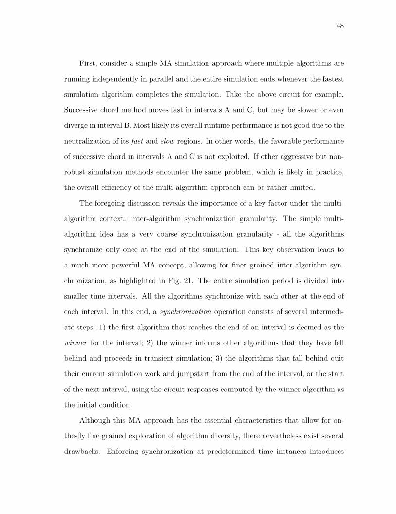
48

First, consider a simple MA simulation approach where multiple algorithms are

running independently in parallel and the entire simulation ends whenever the fastest

simulation algorithm completes the simulation. Take the above circuit for example.

Successive chord method moves fast in intervals A and C, but may be slower or even

diverge in interval B. Most likely its overall runtime performance is not good due to the

neutralization of its fast and slow regions. In other words, the favorable performance

of successive chord in intervals A and C is not exploited. If other aggressive but non-

robust simulation methods encounter the same problem, which is likely in practice,

the overall efficiency of the multi-algorithm approach can be rather limited.

The foregoing discussion reveals the importance of a key factor under the multi-

algorithm context: inter-algorithm synchronization granularity. The simple multi-

algorithm idea has a very coarse synchronization granularity - all the algorithms

synchronize only once at the end of the simulation. This key observation leads to

a much more powerful MA concept, allowing for finer grained inter-algorithm syn-

chronization, as highlighted in Fig. 21. The entire simulation period is divided into

smaller time intervals. All the algorithms synchronize with each other at the end of

each interval. In this end, a synchronization operation consists of several intermedi-

ate steps: 1) the first algorithm that reaches the end of an interval is deemed as the

winner for the interval; 2) the winner informs other algorithms that they have fell

behind and proceeds in transient simulation; 3) the algorithms that fall behind quit

their current simulation work and jumpstart from the end of the interval, or the start

of the next interval, using the circuit responses computed by the winner algorithm as

the initial condition.

Although this MA approach has the essential characteristics that allow for on-

the-fly fine grained exploration of algorithm diversity, there nevertheless exist several

drawbacks. Enforcing synchronization at predetermined time instances introduces

49

unnecessary inflexibility between the algorithms, particularly, when the time step is

controlled independently. It is also difficult to decide the optimal synchronization

granularity, the interval length, a priori. In HMAPS, a more flexible and concep-

tually cleaner synchronization model is adopted. Conceptually, the algorithms do

not directly interact with each other, rather, they asynchronously, or independently,

communicate with a global synchronizer as shown in Fig. 22. The global synchronizer

stores the circuit solutions at the k most time points, where k is determined by the

highest order of numerical integration formula used. With a communication granular-

ity controlled on a individual algorithm basis, each algorithm independently updates

the circuit solutions stored in the global synchronizer contingent upon the timeliness

of its work, and/or loads the most updated initial condition from the synchronizer to

start new work. Compared with the MA approach in Fig. 21, the use of the global

synchronizer provides a more transparent interface between multiple algorithms and

has a clear advantage when high-order integration methods are employed, as detailed

in subsection 7.

t

Continue or update the solutions viaglobal synchronizer

Quit & restart frombetter initial conditions computedby other algorithms

Algorithm-1

Algorithm-2

Algorithm-3

Fig. 22. Synchronization scheme in HMAPS.

50

The global synchronizer in the above MA approach is essentially a coarse grained

communication scheme which enables solution sharing between algorithms. Algo-

rithm diversity is naturally exploited when the best performing algorithm at every

time point writes its latest solution into the global synchronizer. Every algorithm

reads the global synchronizer to get the latest solution as its initial condition for

future time points. Since the write/read operations in the shared-memory based

communication scheme is easy to implement and inexpensive, we can introduce more

beneficial cooperations between algorithms. For example, the selection of the fixed

Jacobian matrix is the most critical point to the performance of the successive chord

method, which is one of the simulation algorithms included under HMAPS. Since

Newton’s method is also used in our MA approach, and it consistently updates its

Jacobian matrix, successive chord method can use the latest Jacobian matrix com-

puted by Newton’s method. The latest Jacobian matrix will make the successive

chord method more likely to converge or converge in less number of iterations. This

inter-algorithm matrix sharing is another communication scheme besides the solution

sharing in HMAPS.

Since there is a predictable trend that the number of cores of multi-core pro-

cessors will keep increasing, we can accommodate intra-algorithm fine grained paral-

lel approaches into the MA framework so that the hardware resources can be fully

utilized and the performance can be further increased. Each algorithm in the MA

approach uses parallel matrix solver [37] to solve the linear equation system during

the nonlinear iterations and parallel device evaluation when evaluating the expen-

sive mosfet model for large number of transistors. This combination of high-level

MA parallelism and low-level fine grained parallel approaches forms the hierarchical

MAPS. Table III compares MAPS [40] and HMAPS. Note that the parallel efficiency

achieved through inter-algorithm parallelisms comes at the expense of more mem-

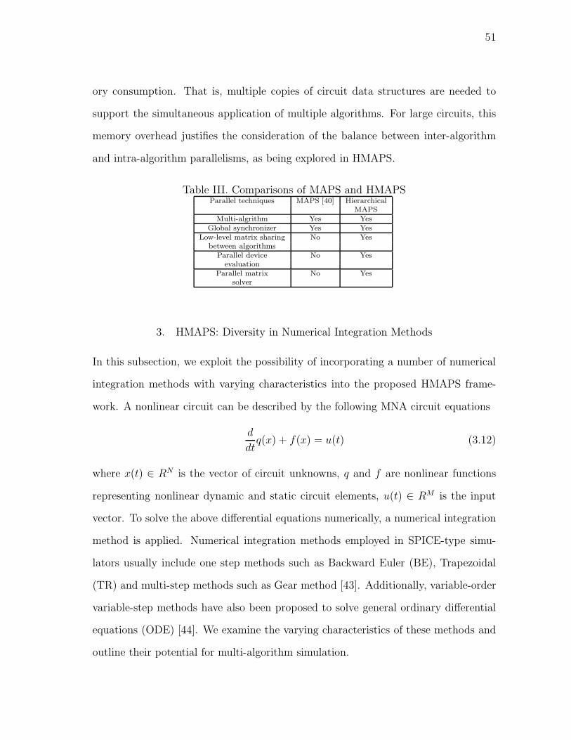
51

ory consumption. That is, multiple copies of circuit data structures are needed to

support the simultaneous application of multiple algorithms. For large circuits, this

memory overhead justifies the consideration of the balance between inter-algorithm

and intra-algorithm parallelisms, as being explored in HMAPS.

Table III. Comparisons of MAPS and HMAPSParallel techniques MAPS [40] Hierarchical

MAPSMulti-algrithm Yes Yes

Global synchronizer Yes YesLow-level matrix sharing No Yes

between algorithmsParallel device No Yes

evaluationParallel matrix No Yes

solver

3. HMAPS: Diversity in Numerical Integration Methods

In this subsection, we exploit the possibility of incorporating a number of numerical

integration methods with varying characteristics into the proposed HMAPS frame-

work. A nonlinear circuit can be described by the following MNA circuit equations

d

dtq(x) + f(x) = u(t) (3.12)

where x(t) ∈ RN is the vector of circuit unknowns, q and f are nonlinear functions

representing nonlinear dynamic and static circuit elements, u(t) ∈ RM is the input

vector. To solve the above differential equations numerically, a numerical integration

method is applied. Numerical integration methods employed in SPICE-type simu-

lators usually include one step methods such as Backward Euler (BE), Trapezoidal

(TR) and multi-step methods such as Gear method [43]. Additionally, variable-order

variable-step methods have also been proposed to solve general ordinary differential

equations (ODE) [44]. We examine the varying characteristics of these methods and

outline their potential for multi-algorithm simulation.

52

Backward Euler and Trapezoidal are one-step integration methods in that they

rely on the availability of the circuit solution at one preceding time point. They are

defined as , xn+1 = xn + hn+1x′n+1 and xn+1 = xn + hn+1

2(x′n + x′n+1), respectively.

The local truncation errors (LTEs) at time tn+1 introduced by BE and TR are

given as

LTEBE = −h2n+1

x′′(ξ)

2, LTETR = −h3

n+1

x′′′(ξ)

12(3.13)

where tn ≤ ξ ≤ tn+1. Variable time steps are used in SPICE simulators to improve

the runtime efficiency [43]. And local truncation error can be used to predict the

variable time step during the simulation. Take Backward Euler method for example,

if solutions at tn are computed, the next time step hn+1 can be computed as

hn+1 =

√

2ǫ

x′′(ξ)(3.14)

where hn+1 = tn+1−tn, ǫ is the user-defined bound for LTE, and x′′(ξ) is computed by

the second order divided difference DD2(tn) since solutions at tn are available. After

xn+1 is computed using hn+1, we can again use LTE formula (3.13) to decide whether

it should be accepted or re-computed. If LTE at tn+1 is within the given bound,

xn+1 is accepted, otherwise xn+1 needs to be re-computed using a smaller timestep.

In Trapezoidal method, the same time step control mechanism may be used except

that equation (3.14) should be replaced accordingly. For nonlinear circuits, slight

modification of the error bound in (3.14) is needed in order to avoid the timestep

“lock up” situation. Readers may refer to [43] for detailed explanation.

In comparison, we note that TR tends to have larger time steps than BE given

the same error bound. However, TR may cause self-oscillation and for stiff circuits

the timestep may need to be reduced. In some cases, numerical integration has to be

switched from TR to the more robust BE to maintain stability.

53

Gear methods [45] provide a different speed vs. robustness tradeoff compared

to the two methods described above. It has been shown that the first and second

order Gear methods are stiffly stable, hence they do not cause self-oscillation. Gear

methods are a family of multistep methods which rely on the circuit solutions at

multiple preceding time points. For example, the fixed time step size second order

Gear method (Gear2) is given by xn+1 = 43xn −

13xn−1 + 2

3hn+1x

′n+1.

If variable timesteps are used, the coefficients in the above formula will be decided

dynamically. The variable timestep Gear2 formula is [46]

xn+1 = −xn−1

h2n+1

hn(2hn+1 + hn)+ xn

(hn+1 + hn)2

hn(2hn+1 + hn)

+x′n+1

hn+1(hn+1 + hn)

2hn+1 + hn

(3.15)

where hn+1 = tn+1 − tn, hn = tn − tn−1. The local truncation error of (3.15) is

LTEGear2 = −h2

n+1(hn+1 + hn)2

6(2hn+1 + hn)x′′′(ξ), (3.16)

where tn ≤ ξ ≤ tn+1. In practise, if the magnitude of LTE exceeds an upper bound,

the stepsize is halved and solutions at xn+1 is recomputed; if the magnitude of LTE is

less than a lower bound, the stepsize is doubled. The lower and upper bound have to

be chosen carefully so that less solution re-computations are needed so as to maintain

a desirable accuracy level [46].

It is possible to integrate even more sophisticated high order methods into

HMAPS. Since only the first and second order Gear method are stiffly stable, higher

order Gear methods are not usually used in SPICE. However, there do exist other

robust high order integration methods. Despite the less familiarity to the CAD com-

munity, they have gained great success in the area of numerical analysis and scientific

computing. High order integration methods (order higher than two) could potentially

54

produce large time steps. However, it is well known that high order methods are un-

stable for some ODE’s. If a constant high order integration method, say fifth order,

is used to solve a stiff system, the step size could be reduced to be very small in order

to maintain stability. Hence, most of the efficient high order integration methods

have certain mechanisms to dynamically vary the order as well as time step. Among

these, DASSL [44] is one of the most successful ones. DASSL uses the fixed leading

coefficient BDF formulas [47] to solve differential equations.

DASSL incorporates a predictor and corrector to solve an ODE system. The

predictor essentially provides an initial guess for the solution and its derivative at a

new time point tn+1. For a kth order DASSL formula, a predictor polynomial ωPn+1 is

formed by interpolating solutions at the last k + 1 time points: (tn−k, · · · , tn−1, tn),

ωPn+1(tn−i) = xn−i, i = 0, 1, · · · , k. (3.17)

The predictor of x and x′ at tn+1 are obtained by evaluating the predictor polynomial

at tn+1

x(0)n+1 = ωP

n+1(tn+1), x′(0)n+1 = ω′P

n+1(tn+1). (3.18)

The predictor of xn+1 and x′n+1 are specially given by the following somewhat involved

interpolation scheme

x(0)n+1 =

k+1∑

i=1

φ∗i (n), x

′(0)n+1 =

k+1∑

i=1

γi(n + 1)φ∗i (n) (3.19)

55

where

ψi(n+ 1) = tn+1 − tn+1−i, i ≥ 1

αi(n+ 1) = hn+1/ψi(n + 1), i ≥ 1

β1(n+ 1) = 1

βi(n+ 1) =ψ1(n+ 1)ψ2n + 1 · · ·ψi−1(n+ 1)

ψ1(n)ψ2n · · ·ψi−1(n), i > 1

φ1(n) = xn

φi(n) = ψ1(n)ψ2(n) · · ·ψi−1(n)DD(xn, xn−1, · · ·

, xn−i+1), i > 1

γ1(n+ 1) = 0

φ∗i (n) = βi(n+ 1)φi(n)

γi(n+ 1) = γi−1(n+ 1) + αi−1(n + 1)/hn+1, i > 1

and DD(xn, xn−1, · · · , xn−i+1), i > 1 is the ith divided difference. The above inter-

mediate variables are computed by using the solutions and time points before tn+1.

The corrector polynomial ωCn+1 is a polynomial which satisfies following condi-

tions: first, it interpolates the predictor polynomial at k equally spaced time points

before tn+1,

ωCn+1(tn+1 − ihn+1) = ωP

n+1(tn+1 − ihn+1), 1 ≤ i ≤ k, (3.20)

where hn+1 is the predicted timestep for tn+1; second, the solution of the corrector

formula is the solution at tn+1,

ωCn+1(tn+1) = xn+1 (3.21)

By following the above two conditions, the corrector of the kth order DASSL formula

56

is given by

αs(xn+1 − x(0)n+1) + hn+1(x

′n+1 − x

′(0)n+1) = 0 (3.22)

where αs =k∑

j=1

1j

.

Then (3.22) is solved together with (3.23) to get the solutions at tn+1.

F (tn+1, ωCn+1(tn+1), ω

′Cn+1(tn+1)) = 0. (3.23)

DASSL uses local truncation error as a measure to control the stepsize as well

as the order. It estimates what the local truncation errors at tn would have been if

the step to xn were taken at orders k − 2, k − 1, k and k + 1, respectively. Based

on these error estimates, DASSL decides the order k′ for the next time step. If xn is

accepted, k′ will be used to compute the solutions at the future time point tn+1; if

xn is rejected, k′ will be used to re-compute xn. Due to the page limit and topic of

interest of this paper, we will not discuss the order and stepsize selection strategy of

DASSL in detail. Readers may refer to [44] for the complete discussion.

The basic procedure of DASSL can be stated as:

1. Calculate solutions at tn using predicted timestep hn, where hn = tn − tn−1;

2. Based on the error estimates at tn, decide order k′ for the next step;

3. Based on LTE at tn, decide whether xn should be accepted or re-computed.

4. Predict the next timestep: hn+1 if xn is accepted; a new hn if xn is re-computed.

From the foregoing discussion, it is evident that numerical integration methods

vary in complexity, speed and robustness. The one-step first-order BE method, is

robust, but has large LTEs. Variable-order variable-step size methods (e.g. DASSL)

have much smaller LTEs and potentially lead to much lager time steps. However,

57

they are significantly more complex and require numerous additional computations

and checks to maintain accuracy and stability. For stiff circuits or stiff periods of the

simulation, variable-order methods may decrease their orders to first order in order

to ensure stability after attempting to stay at higher orders. Under these cases, a

large amount of computed work may be rejected and wasted.

On the other hand, in practice it is difficult to choose a single optimal numerical

integration method for a simulation task a priori. The efficiency of a method is

decided by the nature of the circuits and input stimulus, and it varies over the time as

the circuit passes through various regimes. To this end, HMAPS favorably allows for

on-the-fly interaction of integration methods with varying order and time step control,

at a controllable communication granularity, so as to achieve the optimal results via

collaborative effort dynamically. In particular, as will be seen in subsection 7, our

algorithm synchronization scheme is completely transparent regardless of the choice of

numerical integration and allows for the integration of arbitrary numerical integration

methods.

4. HMAPS: Diversity in Nonlinear Iterative Methods

The nonlinear iterative methods are essential to nonlinear (e.g. transistor) circuit

analysis. Besides the standard Newton-Raphson method, a variety of other choices

exist, providing orthogonal algorithm diversity to numerical integration algorithms

that can be exploited in HMAPS.

The widely used Newton’s method solves a set of nonlinear circuit equations

F(v) = 0 iteratively as follows

J(k)∆v(k) = −F(v(k)) (3.24)

v(k+1) = v(k) + ∆v(k) (3.25)

58

where at the k-th iteration, J(k) is the Jacobian matrix of F, which needs to be

updated at every iteration; ∆v(k) is the solution increment; v(k) and v(k+1) are

the solution guesses at the k-th and (k + 1)-th iterations, respectively. Despite its

good robustness, Newton’s method tends to be expensive. At each iteration, a new

Jacobian matrix J(k) is assembled, which requires expensive computation of device

model derivatives. Note that derivative computation is much more expensive than

the evaluation of device equations and dominates the overall device model evaluation.

Moreover, at each iteration a new matrix solve is required to factorize the updated

Jacobian matrix J(k), which is expensive, especially for large circuits.

Different from Newton’s method, successive chord method is a constant Jacobian

matrix type iterative method [48]. Since a fixed Jacobian matrix Jsc ∈ RN×N is

constructed only once and then used throughout the simulation, no device model

derivatives need to be computed to update the Jacobian matrix during each nonlinear

iteration. As a result, there is a significant reduction in device model evaluation.

Additionally, the fixed Jacobian matrix Jsc is only factorized once and the LU factors

can be reused to solve (3.24) efficiently. However, the downside of not updating

the Jacobian matrix is that the convergence rate of successive chord method is linear,

which is inferior to the quadratic convergence rate of Newton’s method. The selection

of chord values (entries in the Jacobian matrix corresponding to transistors) is very

critical to the performance of successive chord method. Bad chord selection may

lead to excessive number of iterations or even divergence. The convergence criteria

of successive chord method [48] is

∥

∥I− J−1

scJF(v∗)

∥

∥ ≤ 1, (3.26)

where I is the N × N identity matrix, Jsc is the constant Jacobian matrix used in

successive chord method, JF(v∗) ∈ RN×N is the exact Jacobian matrix at solution

59

v∗, of F(v) = 0.

In principle, secant method provides a different efficiency vs. complexity tradeoff

compared with the above two methods. Secant method does form a new Jacobian

matrix at each iteration, but does so approximately. The Jacobian matrix at the k-th

iteration is approximated by Ak in (3.28):

A0 = J(v(0)) (3.27)

Ak = Ak−1 +1

STS(Y −Ak−1S)ST (3.28)

where S = v(k) − v(k−1) and Y = F(v(k))− F(v(k−1)), v(k) and v(k+1) are the solu-

tion guesses at the k-th and (k+1)-th iterations. Secant method also avoids the need

for device model derivative computation. However, a new factorization of Ak is still

needed at every iteration. Secant method has a superlinear convergence rate which

is also inferior to the quadratic convergence rate of Newton’s method.

Although other types of nonlinear iterative methods (e.g. nonlinear relaxation

methods) can also be considered, the three methods discussed above already show

distinguishing tradeoffs between per iteration cost vs. number of iterations, and

efficiency vs. robustness. Newton’s method has the highest per-iteration cost: com-

putation of device model derivatives and solve of a new linear system. However, it

has the favorable quadratic convergence rate, which helps reduce the total number

of iterations required for convergence. At each iteration, Secant method relaxes the

need for device model derivatives, but it only has a superlinear convergence rate.

Successive chord has the lowest per-iteration cost as it relaxes the need for both the

device model derivatives computation and factorization of a new Jacobian matrix.

However, it has a linear convergence rate that corresponds to a larger number of iter-

ations required to reach convergence. When the chord values are not chosen properly,

60

successive chord may not even be able to converge. In terms of robustness, Newton’s

method is the most robust while successive chord is the least robust.

Again, in practice it is difficult to choose a single optimal nonlinear iterative

method a priori. The relative performance of a method is determined by a complex

tradeoff between all the above factors in addition to the dependency on the circuit

type, mode of the circuit and input excitations applied. In addition, different method

is likely to prevail during different phases of a transient simulation. HMAPS allows

for a dynamic exploration of superior performances of multiple nonlinear iterative

methods occurring in different phases of the simulation, contributing to the overall

efficiency of the MA approach. We further emphasize the following key points. Being

applied as a standard alone method, the weak convergence property of a non-robust

iterative method can significantly constrain its application [41, 42]. For example, in

successive chord method it is difficult to find near optimal chord values that achieve

good efficiency while guaranteeing the convergence for the entire simulation. As a re-

sults, non-robust methods are usually discarded for general robust circuit simulation.

In HMAPS, since the standard Newton’s method is always chosen as a solid backup,

other non-robust methods no longer have to converge during the entire simulation,

significantly relaxing their convergence constraints. Moreover, non-robust methods

are employed with a rather different objective in HMAPS: they are purposely con-

trolled in an aggressive or risky way to possibly gain large runtime speedups during

certain phases of the simulation. This unique opportunism contributes to possible

superlinear runtime speedup of the parallel multi-algorithm framework.

5. Construction of Simulation Algorithms

In the current implementation of HMAPS, various numerical integration methods are

paired with nonlinear iterative methods to create a pool of simulation algorithms. In

61

terms of numerical integration methods, Backward Euler, Gear2 and our implemen-

tation of DASSL are included. In terms of nonlinear iterative methods, Newton’s

method is chosen as a solid backup and successive chord is included to gain oppor-

tunistic speedup. It is experimentally found that secant method has weak convergence

property and still requires factorizing a new approximated Jacobian matrix at each

iteration. Since it does not provide significant runtime benefit, secant method is

currently not adopted in HMAPS. The three numerical integration methods with in-

dependent dynamic time step control are all paired with Newton’s method to form

three complete simulation algorithms. Hence, the SPICE-like BE + Newton combi-

nation is selected, which provides a basic guarantee for the success of the simulation.

BE is paired with successive chord to create the fourth algorithm. To further

enhance the runtime benefit of successive chord in transient simulation, a dynamic

time step rounding technique [49] is used. The use of a constant Jacobian matrix in

successive chord method reduces the number of matrix factorizations to one for the

complete nonlinear solve at each time point. Note that the exact Jacobian matrix also

depends on the time step in numerical integration method. For example, in Backward

Euler, a grounded capacitor of value c contributes a stamp c/h to the Jacobian matrix,

where h is the time step. As h is dynamically changed according to dynamic time

step control, the Jacobian matrix varies over the time. To avoid frequent Jacobian

matrix factorizations along the entire time axis, a set of fixed Jacobian matrices are

pre-factorized before the simulation starts at a few geometrically-spaced time steps

hmin, 2hmin, 4hmin, · · · , hmax, where hmin and hmax are estimated min/max time

steps computed by dynamic time step control [49]. The total number of discrete time

steps is given by

1 + ⌈log2(hmax/hmin)⌉ (3.29)

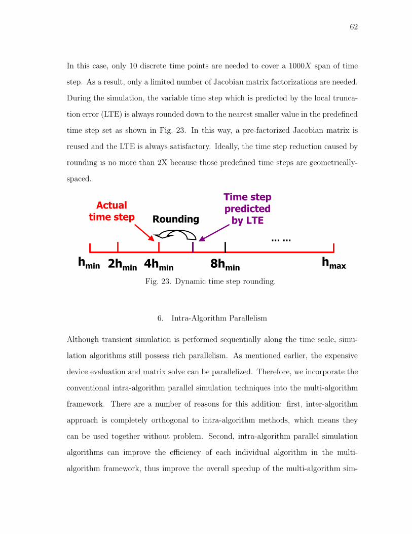
62

In this case, only 10 discrete time points are needed to cover a 1000X span of time

step. As a result, only a limited number of Jacobian matrix factorizations are needed.

During the simulation, the variable time step which is predicted by the local trunca-

tion error (LTE) is always rounded down to the nearest smaller value in the predefined

time step set as shown in Fig. 23. In this way, a pre-factorized Jacobian matrix is

reused and the LTE is always satisfactory. Ideally, the time step reduction caused by

rounding is no more than 2X because those predefined time steps are geometrically-

spaced.

hmin

……

hmax2hmin 4hmin 8hmin

Time step predictedby LTERounding

Actual time step

Fig. 23. Dynamic time step rounding.

6. Intra-Algorithm Parallelism

Although transient simulation is performed sequentially along the time scale, simu-

lation algorithms still possess rich parallelism. As mentioned earlier, the expensive

device evaluation and matrix solve can be parallelized. Therefore, we incorporate the

conventional intra-algorithm parallel simulation techniques into the multi-algorithm

framework. There are a number of reasons for this addition: first, inter-algorithm

approach is completely orthogonal to intra-algorithm methods, which means they

can be used together without problem. Second, intra-algorithm parallel simulation

algorithms can improve the efficiency of each individual algorithm in the multi-

algorithm framework, thus improve the overall speedup of the multi-algorithm sim-

63

ulation. Third, the combination of inter-algorithm and intra-algorithm parallelism

creates more parallelism and is capable of utilizing more cores than inter-algorithm

parallelism alone. By combining the multi-algorithm framework and intra-algorithm

parallel simulation techniques, we form the complete HMAPS approach.

During each iteration of the nonlinear equation solving, circuit elements in the

circuit are evaluated. In parallel device evaluation, the cost of evaluating all circuit el-

ements is divided equally among cores used in parallel device evaluation. In transistor

dominant circuits, mosfet devices are the most time-consuming part to be evaluated.

Therefore, they are divided equally among cores being used. In interconnect dominant

circuits, linear elements are also important. In HMAPS, each simulation algorithm

uses multiple threads to do parallel device evaluation. The total number of threads

used in parallel device evaluation by all algorithms does not exceed the number of

cores on the machine.

Within each iteration of the nonlinear equation solving, a system of linear equa-

tions (3.24) needs to be solved. Earlier circuit simulators use sparse 1.3 or other

sparse matrix solvers designed for circuit simulation. In this paper, we use parallel

matrix solver SuperLU [37] to solve the system of linear equations. SuperLU is a gen-

eral purpose parallel matrix solver with parallel computing capability. It has three

versions: SuperLU for sequential machines; SuperLU MT for shared memory par-

allel machines; SuperLU DIST for distributed memory. SuperLU MT uses threads

for parallel processing while SuperLU DIST uses MPI for interprocess communica-

tion. Based on our thread based HMAPS implementation, we choose SuperLU MT

for parallel matrix solve. Although SuperLU MT is not specifically built for circuit

simulation, it is sufficient for the purpose of verifying our proposed ideas and algo-

rithms. We can easily incorporate any new parallel matrix solver in our simulation

framework.

64

In HMAPS, SuperLU needs to be used with extreme caution since global and

static variables may cause false data sharing between different simulation algorithms

when multiple algorithms are calling the parallel matrix routines simultaneously.

Again, the total number of threads used in parallel matrix solve by all algorithms

does not exceed the number of cores on the machine.

An interesting problem in parallel computing is load balancing and resource allo-

cation. Algorithm designers face challenge of optimally assigning hardware resources

to different tasks in a parallel algorithm. In HMAPS, since each algorithm can utilize

more than one core for low-level parallelism, we need to allocate the cores to each

algorithm optimally to achieve good results.

In HMAPS, we favor the more effective algorithms when allocating the cores. We

follow the experimental observations to decide which algorithm is likely to contribute

more in HMAPS if given more cores for its low-level parallelism. This algorithm will

be given more cores than other algorithms in HMAPS in the hope that this specific

core allocation will result in a overall better performance of HMAPS.

Right now, the core allocation in HMAPS is done manually. Automatic core

assignment is possible if we can predict the performance of HMAPS with any core as-

signment. However, this would require us to build the performance model of HMAPS.

This is an interesting future research direction.

Since the hardware resources (e.g. number of cores, memory) on multi-core

processor computers are limited, tradeoff between inter-algorithm and intra-algorithm

parallelism exists. In thread based implementation of HMAPS, each algorithm is

initiated by one thread and it has to use it own private data structure including

device list, matrices, device models, etc. Otherwise, false data sharing will happen.

Therefore, the memory usage of the 4-algorithm HMAPS is larger than a sequential

algorithm. For circuits of very large size, memory could become a bottleneck. Take

65

the full-chip simulation as an example, simulating the entire chip using one algorithm

is already challenging, replicating the data structure four times will certainly put a

huge burden on the memory. If memory is fully occupied, the increase of read/write

operations on the hard disk will result in performance degradation. In this case, it

would be better to use less number of algorithms in HMAPS and assign more cores

to each algorithm. On the other hand, if the circuit size is small, intra-algorithm

parallelism may not be as beneficial and memory storage is not a limiting factor,

more emphasis can be put on the inter-algorithm parallelism.

Another important issue is the contention on cache and memory bus bandwidth.

If several threads in HMAPS are doing potentially non-useful work, they would still

compete for the cache and memory bandwidth. This contention would deteriorate

the cache and memory condition of all threads in the system, therefore, deteriorate

the performance of HMAPS as a whole.

All the above issues have to be considered when making the proper selection of

algorithms and core assignment in HMAPS. Based on our previous simulation exper-

iments, SC method is likely to contribute the most in HMAPS. Therefore, we assign

4 cores to it in HMAPS. All the other three algorithms use 1 core each. Automatic

algorithm selection and core assignment is possible with the performance model of

HMAPS. We are currently working on performance modeling of HMAPS.

7. Communications in HMAPS

To ensure algorithm diversities are well exploited during the transient simulation and

all algorithms are properly synchronized, a number of guidelines are followed:

• The latest circuit solutions computed by the fastest algorithm shall be passed

to all the slower algorithms as quickly as possible so that slower algorithms can

66

Algorithm-1

Solutions

Jacobian

matrix

Data

Matrix

solve

Device

evaluation

Routines

Algorithm-2

Solutions

Jacobian

matrix

Data

Matrix

solve

Device

evaluation

Routines

…

Algorithm-n

Solutions

Jacobian

matrix

Data

Matrix

solve

Device

evaluation

RoutinesProc1:Solve()

Proc2:Solve()

Proc3:Solve()

mutex

Circuit solution vectors at the K most recent time points

HeadTail

Jacobian

Matrix (t)

Load and Update

WriteRead

Proc1:

Eval()

Proc2:

Eval()

Proc3:

Eval()

Fig. 24. Communication scheme in HMAPS.

use them as initial conditions and keep up with the fastest algorithm;

• Every algorithm has the chance to contribute to the overall performance of

HMAPS as long as it completes certain useful work fast enough;

• Sufficient information shall be shared among all algorithms so that every algo-

rithm has the initial conditions it needs to move forward;

• Synchronization shall be independent of the number and choice of algorithms

(e.g. the order of the numerical integration method);

• Race condition must be avoided during synchronization.

We achieve all of these goals with the aid of a global synchronizer, which is visible

to all algorithms as shown in Fig. 24. It contains circuit solutions at k most recent

time points, where k is decided by the highest numerical integration order used among

67

all the algorithms. In HMAPS, k is set to be 6 since the highest integration order

used in our DASSL implementation is 5. The head and tail of these k time points

are denoted as thead and ttail (thead > ttail), respectively. Each algorithm works on its

own pace, and independently or asynchronously accesses the global synchronizer via

a mutex guard which prevents the potential race condition. Hence, there is no direct

interaction between the algorithms. When one algorithm finishes solving one time

point, it will access the global synchronizer (the frequency of access can be tuned).

If its current time point talg. is ahead of the head of the global synchronizer, i.e.

talg. > thead, the head is updated by this algorithm to talg. and the tail of the global

synchronizer is deleted. In this way, the global synchronizer still maintains k time

points and circuit solutions associated with them. If this algorithm does not reach as

far as the head, but it reaches a time point that is ahead of the tail, the new solution

is still inserted into the synchronizer and the tail is deleted. Additionally, before

each algorithm starts to compute the next new time point, it also checks the global

synchronizer to load the most recent initial conditions stored in the synchronizer so

as to move down the time axis as fast as it can.

The pseudocode of the synchronization algorithm is listed below Algorithm 2.

Every simulation algorithm in HMAPS uses Algorithm 2.

One favorable feature of this synchronization scheme is that it provides a trans-

parent interface between an arbitrary number of algorithms with varying character-

istics (e.g. independent dynamic time step control and varying numerical integration

order): the algorithms do not talk to each other directly, rather, through the global

synchronizer, they assist each other in a best possible way so as to collectively advance

the multi-algorithm transient simulation. The communication overhead of the scheme

is quite low. Each algorithm accesses the global synchronizer only after solving the

entire solution solution(s) at one (or several) time point(s). Moreover, no algorithm

68

is idle at any given time in this scheme, which avoids the time wasted in waiting,

possibly in a direct synchronization scheme.

Algorithm 2 Synchronization algorithm

1: while simulation not over do

2: Mutex lock.3: if talg. > thead then

4: Update global synchronizer.5: else if thead > talg. > ttail then

6: Insert solution into global synchronizer.7: Read global synchronizer as initial condition.8: else

9: Read global synchronizer as initial condition.10: end if

11: Mutex unlock.12: Solve for next time point.13: Update talg. and its solution.14: end while

The above communication scheme is essentially inter-algorithm solution shar-

ing. Since the communication cost is very low on the shared-memory based platform,

we can have more beneficial interactions between algorithms to further improve the

overall performance of HMAPS. According to (3.26), the fixed Jacobian matrix Jsc is

critical to the performance of successive chord method. If Jsc is close to the current

true Jacobian matrix, successive chord method will converge, otherwise it will prob-

ably diverge. During the transient simulation, circuit responses as well as the true

Jacobian matrix are changing. For example, within interval A and C in Fig. 20, the

circuit responses as well as the Jacobian matrix are not changing, therefore, successive

chord method will proceed very fast. Within interval B, since the circuit responses

and the Jacobian matrix is changing rapidly, successive chord method is likely to slow

down or diverge. So using a fixed Jacobian matrix Jsc for the entire simulation period

69

in successive chord method is not good. Since Newton’s method is used in HMAPS,

successive chord method can use the latest Jacobian matrix computed by Newton’s

method if its performance starts to degrade. In this way, successive chord method

can always use a better Jsc on-the-fly and there is no need to manually choose chord

values.

We also summarize the overall structure of HMAPS in Fig. 25. As a reference,

the overall structure of MAPS is shown in Fig. 26 where only coarser-grained inter-

algorithm parallelism is used. It shall be noted this multi-algorithm parallel paradigm

is not only applicable to circuit simulation. It is possible to extend it to exploit

algorithm diversity in a variety of parallel CAD applications.


We demonstrate various aspects of HMAPS including runtime speedup, accuracy,

synchronization overhead and the global synchronizer. As discussed in subsection 5,

we have four simulation algorithms in the current implementation of HMAPS: New-

ton’s method + Backward Euler, Newton’s method + Gear2, Newton’s method +

DASSL and successive chord method + dynamic time step rounding. In HMAPS,

each algorithm is also capable of utilizing parallel device evaluation and parallel ma-

trix solvers. Besides the four-algorithm HMAPS, we also implement the sequential

version of these four simulation algorithms and HMAPS with inter-algorithm paral-

lelism only as references.

We have two different types of circuits in the experiments. The first type of

circuits (CKT 1, 2, 3, 4) are the transistor dominant combinational circuits; the

second type (CKT 5, 6, 7, 8) is the mesh based clock distribution circuit [8]. For

the first type of circuits, they have very regular structure and large size. They are

dominated by MOSFET transistors. Mesh based clock distribution circuits have large

70

BEBE NewtonNewton

…

Numerical integration Nonlinear solving methods

Gear2Gear2

DASSLDASSL

…………

SCSC

SecantSecant

…………

Algorithm-1

Core 1

globalglobal synchronizersynchronizer

Jacobian matrixJacobian matrix

Shared

memory

Core 2 Core 3 Core 4 Core 5 Core 6 Core 7 Core 8

… …

time

HMAPS

Multi-core

processor

Algorithm-2 Algorithm-3

Fig. 25. Overall structure of HMAPS.

71

BEBE

Gear2Gear2

DASSLDASSL

…………

NewtonNewton

SCSC

SecantSecant

…………

…

Algorithm-1 Algorithm-2 Algorithm-3 …………

Simulation Algorithm pool

Core 1Core 1 Core 2Core 2 Core 3Core 3 Core 4Core 4

Algorithm-n

Core nCore n……

Multi-core

processor

MAPS

Numerical integration Nonlinear solving methods

globalglobal synchronizersynchronizerShared

memory

Algorithm-4

Fig. 26. Overall structure of MAPS.

72

number of linear elements and small number of transistors.

The parallel simulation code is multi-threaded using Pthreads. Experiments are

conducted on a Linux server with 8GB memory and two quad-core processors running

at 2.33GHz. It is a SMP (Symmetric multiprocessing) system.

Table IV summarizes the runtime (in seconds) of four sequential algorithms and

HMAPS with inter-algorithm parallelism only. It demonstrates the benefit of inter-

algorithm parallelism in the multi-algorithm framework. There is no intra-algorithm

parallelism in this implementation of HMAPS. Each algorithm is initiated by one

thread, and each thread is running on one cpu core. Therefore, this implementation

of HMAPS uses four cpu cores in total. The runtime speedup of HMAPS is with

respect to the standard SPICE-like implementation: Newton + BE. For 7 out of 8

examples (circuits 2, 3, 4, 5, 6, 7, 8), HMAPS achieves superlinear speedup (larger

than 4x).

Table IV. Runtime (in seconds) of four sequential algorithms and HMAPS with in-

ter-algorithm parallelism only (using 4 threads)HMAPS Speedup

CKT Description # of lin. # of Newton Newton Newton SC w/ inter- alg. overele. FETs +BE +Gear2 +DASSL parallelism only Newton+BE

1 comb. logic 1 200 400 105.1 25.1 45.8 80.3 33.8 3.11x2 comb. logic 2 1000 2000 947.5 579.5 837.1 123.5 128.3 7.39x3 comb. logic 3 4000 8000 1230.0 879.8 626.0 83.3 94.6 13.0x4 comb. logic 4 8000 16000 3103.1 3109.8 866.6 181.0 207.7 14.9x5 clock mesh 1 10k 20 120.8 34.7 N/A 10.5 11.4 10.6x6 clock mesh 2 20k 40 1231.3 489.0 N/A 62.5 63.6 19.36x7 clock mesh 3 25k 50 4227.0 1547.5 N/A 210.3 220.3 19.19x8 clock mesh 4 29.7k 60 3301.2 2951.9 1184.2 101.0 123.0 26.8x

For larger circuits (circuits 2, 3, 4, 5, 6, 7, 8), successive chord method is the

fastest sequential algorithm. This is because SC method avoids the costs of repeatedly

factorizing large Jacobian matrices and evaluating device model derivatives, which are

especially high for large circuits. For smaller circuit (circuit 1), the advantage of SC

method is smaller since the matrix size is small and there is smaller number of de-

vices, and the contribution in HMAPS is mainly from advanced numerical integration

73

methods (Gear2 and DASSL).

In Table V, we demonstrates the runtime and speedup of HMAPS with inter-

algorithm parallelism only (HMAPS implementation 1 ) and HMAPS with both inter-

algorithm parallelism and intra-algorithm parallelism (HMAPS implementation 2 ).

The last column in Table V includes the data for the speedup of HMAPS imple-

mentation 2 against HMAPS implementation 1. HMAPS implementation 1 has four

algorithms and uses four cores. In HMAPS implementation 2, each algorithm can

utilize many cores to do intra-algorithm parallelism. Due to the limited number of

cores on the machine, we have to assign the available cores wisely. According to

the principle mentioned in subsection 6, we assign four extra threads/cores for SC

method to do parallel device evaluation and parallel matrix solve. Other three algo-

rithms only use one thread/core respectively. Therefore, HMAPS implementation 2

utilizes all eight cores on the machine.

Table V. HMAPS implementation 1 (Inter-algorithm parallelism only, using 4 threads)

vs HMAPS implementation 2 (Inter- and Intra-algorithm parallelism, using

8 threads)# of threads used # of threads used HMAPS HMAPS HMAPS

CKT Description in HMAPS in HMAPS implementation 1 implementation 2 implementation 2implementation 1 implementation 2 runtime runtime speedup

1 comb. logic 1 4 8 33.8s 37.3s 0.91x2 comb. logic 2 4 8 128.3s 94.9s 1.35x3 comb. logic 3 4 8 94.6s 53.2s 1.78x4 comb. logic 4 4 8 207.7s 68.2s 3.05x5 clock mesh 1 4 8 11.4s 19.2s 0.59x6 clock mesh 2 4 8 63.6s 32.5s 1.96x7 clock mesh 3 4 8 220.3s 106.5s 2.07x8 clock mesh 4 4 8 123.0s 61.8s 1.99x

We can see from Table V both implementations of HMAPS achieves good speedup

in general. By creating more parallelism, HMAPS implementation 2 achieves larger

speedup than HMAPS implementation 1 for large circuits (circuit 2, 3, 4, 6, 7, 8).

However, for relatively small circuits (circuit 1, 5), HMAPS implementation 2 does

not improve the runtime compared with HMAPS implementation 1, sometimes, there

74

is even a slow down. This “unexpected” slow down in runtime brings up an interesting

problem in parallel circuit simulation, and even in parallel computing in general, that

is, more parallelism is not always better.

For our particular parallel circuit simulation problem, this situation can be more

carefully analyzed. First of all, the parallelizability of a simulation algorithm can be

limited due to the nature of the algorithm or implementation issues. Take the succes-

sive chord method as an example, the parallel matrix solver [37] we use in HMAPS

implementation 2 does not parallelize the matrix resolve routine which is a major cost

in SC method. Therefore, this implementation issue affects the parallelizability of SC

method so that its runtime does not scale well with the number of cores it uses. In

principle, the matrix resolve routine can be parallelized just as the matrix factoriza-

tion routine. If there is a parallel matrix solver available which can do parallel matrix

resolve, we can improve the performance of SC method as well as HMAPS. Second,

creating parallelism introduces overhead. Each thread is associated with its creation

and termination cost. More threads doing fine-grained parallelism means more mem-

ory access. For smaller circuits, these overhead can not be neglected compared with

the computational cost.

Results in Table V reveal the limitation of low-level parallelism which again

justifies the usefulness of inter-algorithm parallelism. Inter-algorithm parallelism cre-

ates more opportunities for parallel circuit simulation which are impossible to find in

intra-algorithm parallelism.

In Tables VI and VII, we compare HMAPS with the parallel version of New-

ton+Gear2 algorithm. In Table VI, we compare HMAPS implementation 1 (Inter-

algorithm parallelism only, using 4 threads) with Newton+Gear2 algorithm using 1

and 4 threads. Newton+Gear2 using 4 threads can be viewed as a standard way

of parallel circuit simulation. We can see from the last column that HMAPS im-

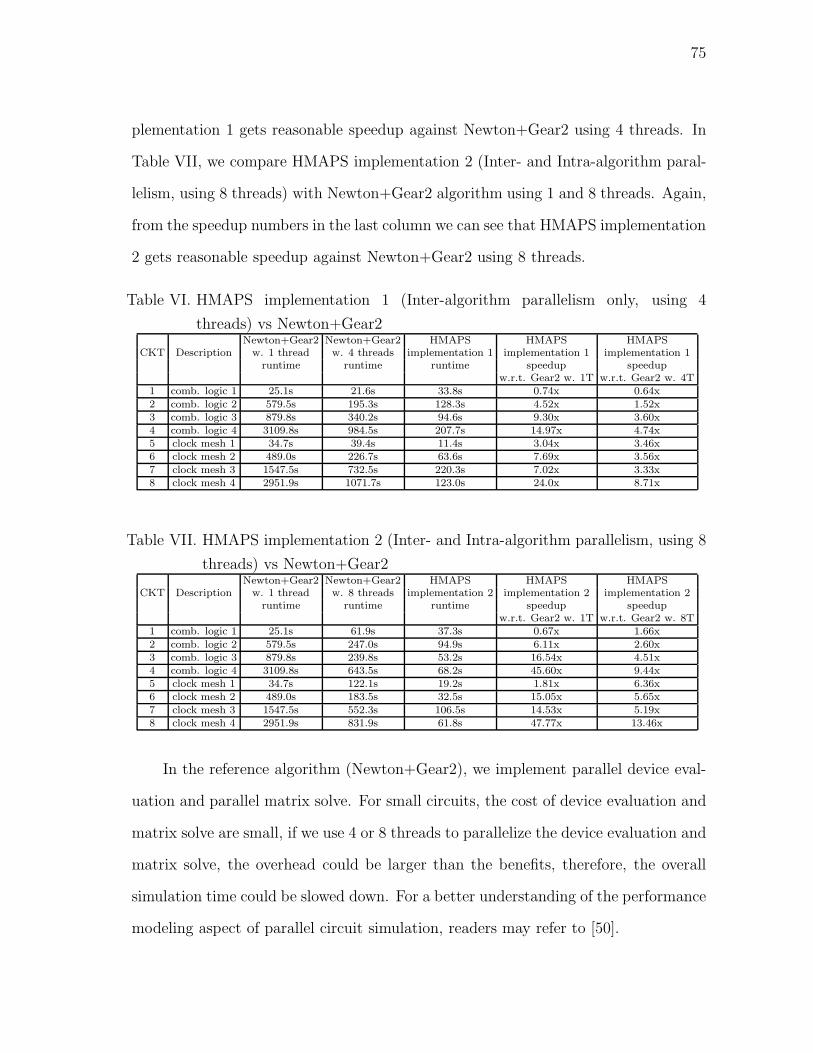
75

plementation 1 gets reasonable speedup against Newton+Gear2 using 4 threads. In

Table VII, we compare HMAPS implementation 2 (Inter- and Intra-algorithm paral-

lelism, using 8 threads) with Newton+Gear2 algorithm using 1 and 8 threads. Again,

from the speedup numbers in the last column we can see that HMAPS implementation

2 gets reasonable speedup against Newton+Gear2 using 8 threads.

Table VI. HMAPS implementation 1 (Inter-algorithm parallelism only, using 4

threads) vs Newton+Gear2Newton+Gear2 Newton+Gear2 HMAPS HMAPS HMAPS

CKT Description w. 1 thread w. 4 threads implementation 1 implementation 1 implementation 1runtime runtime runtime speedup speedup

w.r.t. Gear2 w. 1T w.r.t. Gear2 w. 4T1 comb. logic 1 25.1s 21.6s 33.8s 0.74x 0.64x2 comb. logic 2 579.5s 195.3s 128.3s 4.52x 1.52x3 comb. logic 3 879.8s 340.2s 94.6s 9.30x 3.60x4 comb. logic 4 3109.8s 984.5s 207.7s 14.97x 4.74x5 clock mesh 1 34.7s 39.4s 11.4s 3.04x 3.46x6 clock mesh 2 489.0s 226.7s 63.6s 7.69x 3.56x7 clock mesh 3 1547.5s 732.5s 220.3s 7.02x 3.33x8 clock mesh 4 2951.9s 1071.7s 123.0s 24.0x 8.71x

Table VII. HMAPS implementation 2 (Inter- and Intra-algorithm parallelism, using 8

threads) vs Newton+Gear2Newton+Gear2 Newton+Gear2 HMAPS HMAPS HMAPS

CKT Description w. 1 thread w. 8 threads implementation 2 implementation 2 implementation 2runtime runtime runtime speedup speedup

w.r.t. Gear2 w. 1T w.r.t. Gear2 w. 8T1 comb. logic 1 25.1s 61.9s 37.3s 0.67x 1.66x2 comb. logic 2 579.5s 247.0s 94.9s 6.11x 2.60x3 comb. logic 3 879.8s 239.8s 53.2s 16.54x 4.51x4 comb. logic 4 3109.8s 643.5s 68.2s 45.60x 9.44x5 clock mesh 1 34.7s 122.1s 19.2s 1.81x 6.36x6 clock mesh 2 489.0s 183.5s 32.5s 15.05x 5.65x7 clock mesh 3 1547.5s 552.3s 106.5s 14.53x 5.19x8 clock mesh 4 2951.9s 831.9s 61.8s 47.77x 13.46x

In the reference algorithm (Newton+Gear2), we implement parallel device eval-

uation and parallel matrix solve. For small circuits, the cost of device evaluation and

matrix solve are small, if we use 4 or 8 threads to parallelize the device evaluation and

matrix solve, the overhead could be larger than the benefits, therefore, the overall

simulation time could be slowed down. For a better understanding of the performance

modeling aspect of parallel circuit simulation, readers may refer to [50].

76

In Table VIII, we list the cost breakdown for each circuit in terms of device

evaluation, matrix solve and matrix resolve.

Table VIII. Computational component cost (in seconds) breakdown for each example

circuitJacobian

CKT Description matrix Matrix Matrixevaluation solve resolve

1 comb. logic 1 9.8e-3 3.8e-3 6.8e-52 comb. logic 2 7.0e-2 2.9e-1 3.3e-33 comb. logic 3 6.1e-1 2.2e1 5.7e-24 comb. logic 4 2.04 1.85e2 2.3e-15 clock mesh 1 1.3e-2 1.6e-2 4.7e-46 clock mesh 2 1.0e-1 1.5e1 4.0e-27 clock mesh 3 1.8e-1 5.1e1 9.6e-28 clock mesh 4 2.6e-1 8.2e1 1.31e-1

We demonstrate the accuracy of HMAPS in Figs. 27 and 28, where the transient

circuit waveforms simulated by HMAPS are compared with those obtained through

the serial simulation of Newton+BE algorithm. A minimum step size is purposely

chosen in the serial simulation such that the results may be considered as exact. The

results computed by HMAPS are indistinguishable from the exact.

0 1 2 3 4

x 10−9

0

1

2

3

4

5

Time(s)

Vol

tage

(v)

Serial, exactParallel

.

Fig. 27. Accuracy of HMAPS for a combinational logic circuit.

77

0 0.5 1 1.5

x 10−8

4.588

4.5885

4.589

4.5895

Time(s)

Vol

tage

(v)

Serial, exact Parallel

Fig. 28. Accuracy of HMAPS for a double-balanced mixer.

0

20

40

60

80

100

mes

h1

mes

h2

com

b.

log

ic 1

com

b.

log

ic 2

mix

er

lna+

mix

er

Per

cen

tag

e(%

)

synchronization cost other computational cost

Fig. 29. Synchronization cost vs. other computational cost.

78

Each simulation algorithm used in HMAPS has the same convergence check-

ing mechanism to ensure the computed results are accurate. We use both relative

tolerance and absolute tolerance to check the norm of the residual of the system

of nonlinear equations. Therefore, only accurate results are written into the global

synchronizer. The simulation result of HMAPS is always accurate.

Inter-algorithm parallelism in HMAPS has low synchronization overhead due

its coarse-grained nature. In Fig. 29, we compare the overall synchronization cost

associated with the inter-algorithm parallelism and the computational cost. The

synchronization usually takes about 1 ∼ 2% of the total runtime.

We provide real-time profiling data to demonstrate the interactions between the

four algorithms via the global synchronizer. Fig. 30 shows how often each individual

algorithm updates the global synchronizer during the entire simulation in HMAPS.

We can see that each algorithm has the chance to contribute to the global synchro-

nizer. Variations exist across different test circuits. Fig. 31 is a local view of the global

synchronization update within a time window. The y-axis marks the algorithm that

updates the global synchronizer at each time point.

020406080

100

mesh 3 comb.

logic 2

mixer

Per

cen

tag

e(%

)

BE

Gear2

DASSL

SC

Fig. 30. Overall global synchronizer update breakdowns.

79

6.55 6.6 6.65 6.7 6.75

x 10−9

BE

Gear2

DASSL

SC

Time(s)

Fig. 31. Synchronizer updates within a local time window.

In Fig. 32, for the simulation of a clock mesh, we take three snapshots of the

global synchronizer content with the relative time locations of the 6 most recent

circuit solutions marked. As can be seen, the stored 6 solutions may be contributed

by different algorithms and their relative locations evolve over the time.

In Table IX, we list the memory usage for every simulation. We can see that

for a single simulation algorithm, SC method has the largest memory usage. This is

because SC method needs to store multiple pre-factorized Jacobian matrices. HMAPS

has the largest memory usage among all simulation runs. This is expected since four

algorithms in HMAPS use their own private data structure. However, the memory

cost is still under control. For very large circuits, the challenge on the memory storage

could be a potential limitation for HMAPS. On the other and, there are also lots of

practical circuits, the storage requirement is not too demanding, yet the simulation

needs to be speeded up. HMAPS would be a nice fit for such cases. Also, due to

the inherent low communication overhead, HMAPS may be able to solve very large

80

Updated by SC

Updated by Newton+BE

Updated by Newton+DASSL

global synchronizer

Fig. 32. Snapshot of the global synchronizer.

circuits over the network, where each node has sufficient memory to keep a separate

copy of data structures.

Table IX. Memory usage for each simulationNewton Newton Newton Newton Newton

CKT Description +BE SC +DASSL +Gear2 +Gear2 +Gear2 HMAPS HMAPSw. 1T w. 1T w. 1T w. 1T w. 4T w. 8T impl. 1 impl. 2

1 comb. logic 1 22mB 24mB 22mB 22mB 23mB 23mB 25mB 26mB2 comb. logic 2 56mB 94mB 56mB 56mB 57mB 60mB 106mB 115mB3 comb. logic 3 330mB 801mB 330mB 330mB 335mB 340mB 997mB 1.1gB4 comb. logic 4 854mB 854mB 854mB 854mB 859mB 864mB 2.9gB 3.2gB5 clock mesh 1 122mB 128mB 122mB 122mB 122mB 129mB 135mB 137mB6 clock mesh 2 480mB 815mB 480mB 480mB 498mB 501mB 1.1gB 1.1gB7 clock mesh 3 750mB 1.5gB 750mB 750mB 757mB 765mB 2.0gB 2.0gB8 clock mesh 4 682mB 682mB 684mB 684mB 703mB 704mB 2.1gB 2.1gB

There is a lack of debugging tools which fully support multi-threaded based

programs. We take the divide-and-conquer approach in our debugging process. We

first make sure that individual algorithm used in HMAPS are implemented correctly,

then the communication scheme and interactions between algorithms.

81

9. Summary

A novel hierarchical multi-algorithm parallel simulation approach is presented to

achieve efficient coarse grained parallel computing via exploration of algorithm di-

versity. The unique nature of the approach makes it possible to achieve superlinear

runtime speedup and opens up new opportunities to utilize increasingly parallel com-

puting hardware. Additionally, our approach requires minimum parallel programming

effort and allows for reuse of existing serial simulation codes.

A potential limitation of HMAPS is the memory usage. Since HMAPS uses

multiple simulation algorithms and each algorithm has its own data structure, the

memory usage of HMAPS is higher than a single algorithm simulation. On the multi-

core platform where all cores/threads share the memory on a single machine, memory

could become a limiting factor for large circuits. To eliminate this memory limitation,

we can migrate HMAPS onto a distributed computing platform where each simulation

algorithm is running on one local machine and communication is through the net-

work. The inter-algorithm communication/synchronization over the network can be

implemented using message passing in MPI while intra-algorithm parallelism within a

local machine can be implemented in Pthreads. This MPI+Pthreads implementation

of HMAPS for the distributed platforms is an interesting future research topic.

82

CHAPTER IV

CIRCUIT OPTIMIZATION

In order to achieve the clock skew level given by the design specifications, designers

need to perform clock mesh optimization. Optimizing the clock mesh at a desirable

accuracy level requires more effort than clock mesh analysis since multiple simulations

need to be called during the optimization to verify the performance of clock mesh

after tunings. Due to the sheer size of clock mesh, previous attempts on clock mesh

optimization are largely heuristic in nature. In [8], a divide-and-conquer approach

is employed to tune the wire size in the clock mesh. The linear grid is cut into

smaller independent linear networks and each smaller linear network is optimized

in parallel. To compensate for the loss of accuracy induced by cutting the grid,

capacitive loads are smoothed/spreaded out on the grid. Although the runtime of

this approach is manageable, there is no systematic way of controlling the error. In

[16], very fast combinatorial techniques are proposed for clock driver placement. As

an alternative to wire sizing and clock driver placement, clock driver sizing can also

be used in clock mesh optimization. For non-uniform clock load distributions in the

clock mesh, if changing the clock driver placement is impossible due to blockage or

other constraints, changing the sizes of clock drivers can achieve the same or even

better results. In our work, we focus on clock driver sizing.

In many areas of science and engineering, there are a lot of optimization problems

similar to the clock mesh optimization problem which are characterized by objective

function obtained from expensive computer simulations and lack of explicit derivative

information. Standard continuous optimization methods such as sequential quadratic

programming method have many disadvantages in solving this kind of optimization

methods. Due to the lack of explicit derivative information, continuous optimization

83

methods compute the derivative internally by using inefficient numerical differenti-

ation. Furthermore, these methods usually have small incremental step sizes which

make the progress slow. On the other hand, simulated annealing converges to good

final solution given sufficiently long time. And it has been parallelized for CAD prob-

lems before [17]. However, the runtime required by simulated annealing to reach a

good final solution is often considered to be extreme long, thus impractical.

We propose to use asynchronous parallel pattern search (APPS) method [18, 19]

for clock mesh optimization [51]. To the best of our knowledge, this is the first re-

ported attempt to use APPS for physical design optimization. The APPS method

has many advantages over the traditional optimization methods in solving the specific

clock mesh optimization problem. First, no derivative information is needed. Sec-

ond, the pattern search based approach is fully parallelizable and its runtime almost

scales linearly with the number of processors. Third, under mild conditions, APPS is

guaranteed to converge to a local optimum [18, 19] and hence well suited for tuning

of clock driver sizes.

Although the original APPS method is significantly more efficient compared with

other alternative optimization methods, we propose two domain-specific enhance-

ments to further extend its efficiency. Our experimental results show that for the

clock driver sizing problem, APPS method significantly outperforms the traditional

sequential quadratic programming (SQP) based method. Furthermore, our applica-

tion specific enhancements can achieve more than 2x speedup over the original APPS

method.

84

A. Basic Description of APPS

APPS is a derivative free search based optimization method which is best suited for

solving problems whose objective functions are evaluated by complex simulations and

also lack explicit derivative information [18, 19]. APPS solves both unconstrained and

bound constrained nonlinear optimization problems. The bound constrained problem

is given by

minx∈Rn

f(x)

subject to l ≤ x ≤ u (4.1)

Here f : Rn → R and x ∈ Rn, l is a size n vector with entries in R∪ −∞ and u is

a size n vector with entries in R ∪ +∞. APPS can also handle linear constraints.

The complete algorithm is described in Algorithm 3. Notations used in Al-

gorithm 3 are explained as follows: Dk = d(1)k , d

(2)k , . . . , d

(pk)k is the set of search

directions at iteration k, superscripts denote the direction index, which range from 1

to pk at iteration k. ∆(i)k denotes the step length along the ith direction. Ak contains

the indices of search directions that have an associated trial point in the evaluation

queue at the start of iteration k, it may be reset or modified in Step 3 or 4. Ak is

also called “active” set. qmax is the max size of the evaluation queue.

APPS has a manager-worker paradigm and uses MPI to manage the parallel

tasks. There is a single manager processor controlling the optimization flow while

worker processors are doing objective function evaluations.

Fig. 33 is an illustrative example of using APPS for a 2 dimensional case to find

lower function value (darker part). The number of worker processors is assumed to

be three. In the first iteration, we begin with an initial point and generate four trial

points along the four axial directions. Only two of those four points get evaluated in

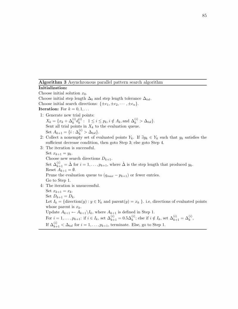
85

Algorithm 3 Asynchronous parallel pattern search algorithmInitialization:

Choose initial solution x0.Choose initial step length ∆0 and step length tolerance ∆tol.Choose initial search directions: ±e1,±e2, · · · ,±en.Iteration: For k = 0, 1, . . .

1: Generate new trial points:

Xk = xk + ∆(i)k d

(i)k : 1 ≤ i ≤ pk, i /∈ Ak, and ∆

(i)k > ∆tol.

Sent all trial points in Xk to the evaluation queue.

Set Ak+1 = i : ∆(i)k > ∆tol.

2: Collect a nonempty set of evaluated points Yk. If ∃yk ∈ Yk such that yk satisfies thesufficient decrease condition, then goto Step 3; else goto Step 4.

3: The iteration is successful.Set xk+1 = yk.Choose new search directions Dk+1.

Set ∆(i)k+1 = ∆ for i = 1, . . . , pk+1, where ∆ is the step length that produced yk.

Reset Ak+1 = ∅.Prune the evaluation queue to (qmax − pk+1) or fewer entries.Go to Step 1.

4: The iteration is unsuccessful.Set xk+1 = xk.Set Dk+1 = Dk.Let Ik = direction(y) : y ∈ Yk and parent(y) = xk . i.e, directions of evaluated pointswhose parent is xk.Update Ak+1 ← Ak+1\Ik, where Ak+1 is defined in Step 1.

For i = 1, . . . , pk+1: if i ∈ Ik, set ∆(i)k+1 = 0.5∆

(i)k ; else if i /∈ Ik, set ∆

(i)k+1 = ∆

(i)k ,

If ∆(i)k+1 < ∆tol for i = 1, . . . , pk+1, terminate. Else, go to Step 1.

86

Fig. 33. An illustrative example of APPS method.

87

iteration one. Since there is a trial point which provides sufficient decrease of the ob-

jective value, it becomes the starting point of iteration 2. In the second iteration, four

more points are generated. Unlike the previous iteration, we find that no evaluated

trial point decreases the objective function value. Hence, the unsuccessful direction

from the current iteration is step reduced and re-evaluated in iteration 3.

B. Quick Estimation

For the clock driver sizing problem, since the objective is to minimize clock skew, we

define f(x) as a performance metric for clock skew:

f(x) =∑

j∈S

(Tj − µ)2 (4.2)

where x is the vector containing the sizes of all clock drivers, Tj is the clock arrival

time at sink node j, S is the set contains all sink nodes, µ = (∑

j∈S Tj)/ |S| is the

average of all T s.

The purpose of the optimization is to find an optimal set of clock driver sizes to

minimize f(x). There are only axial search directions in the original APPS method,

which means each direction either sizes up or down only one clock driver. Apart from

providing the initial clock driver sizes, we also provide an initial step length ∆0. A

large initial step length will result in large change in driver sizes. For the purpose of

fine local tuning, it is better to have a well-controlled initial step size.

In the clock driver sizing problem, in order to evaluate the objective function

f(x) for a trial point x′, we have to do an accurate transient simulation for the entire

clock mesh using driver sizes in the vector x′. The transient simulation of the clock

mesh is the most time consuming part in the entire optimization flow.

We propose to use a quick estimation method to identify a smaller set of good

88

trial points, thus effectively reducing the number of full evaluations at each iteration.

Before we run the accurate simulation, all trial points are going through a quick

estimation step. This quick estimation step is like a “virtual evaluation” step in

which we estimate the objective function value for all trial points quickly. After the

estimated objective function value for all trial points are obtained, we sort them.

Trial points with smaller estimated objective function values will be placed before

trial points with larger estimated objective function values in the evaluation queue.

So, trial points will be sent to available worker processors in the ascending order of

the estimated objective function value.

Since we rank trial points after quick estimation, capturing the relative difference

in the objective function value between trial points is important. Despite the fact

that the quick estimated objective function values have some error, the chance for a

successful trial point to be among the top ranked points is very high.

The quick estimation method is similar to the driver merging method and harmonic-

weighted model order reduction method proposed in [26]. For fast clock mesh simu-

lation, we want to use model order reduction to reduce the size of the linear mesh.

1. Driver Merging

The bottleneck in the standard model order reduction algorithm is the large number

of ports of the linear part. Therefore, we need to aggressively reduce the number of

ports of the linear part of the clock mesh by using the driver merging method. After

the number of drivers is drastically reduced, we can apply the harmonic-weighted

model order reduction [26] to simulate the simplified clock mesh. As a result, two

orders of magnitude of speedup and certain level of accuracy are achieved by the

quick estimation routine.

The driver merging is done by exploiting the locality in the clock mesh. In the

89

driver merging step, the modified driver is retained as is so that the effect of its size

change is captured. All the other drivers are merged into fewer number of super

drivers according to their geometric locations on the clock mesh. For example, if

5 drivers are close together, we merge them into one super driver whose size is the

sum of all 5 drivers. The geometrical location of this super driver is the weighted

center location of those 5 drivers. In other words, the super driver will be placed

closer to larger drivers to reflect their relatively larger influence in the original clock

mesh. The driver merging scheme is formulated in (4.3). S is the size of a driver; L

is the location of a driver, which can be represented by its coordinates in the X-Y

coordinate system. Driver j through driver k are merged into a new driver with size

Snew and location Lnew. This driver merging approach is illustrated in Fig 34.

Snew =k

∑

i=j

Si, Lnew =k

∑

i=j

Si

Snew

Li (4.3)

Modified clock driver Super drivers

Driver

merging

Kept here

Fig. 34. Driver merging method where modified clock driver is kept.

Another more aggressive driver merging approach can also be used. In this

approach, there will be only one merging scheme for one clock mesh no matter which

90

driver is modified. This approach is illustrated in Fig. 35. The effect of individual

gate change can still be kept. For example, if two adjacent drivers are modified in

two trial points respectively, since their sizes are different, the location of super driver

into which these two drivers are merged will be different in these two cases. So the

relative difference between trial points is still captured.

Modified clock driver,

merged

Super drivers

Driver

merging

Fig. 35. Driver merging method where modified clock driver is merged.

In the driver merging, there is a tradeoff between the speedup and accuracy. More

super drivers in the resulting simplified clock mesh means better accuracy and worse

runtime while less super drivers in the simplified clock mesh means worse accuracy

and better runtime.

2. Harmonic Weighted Model Order Reduction

We use harmonic weighted model order reduction to simulate the resulting simplified

clock mesh. In the harmonic weighted model order reduction, a multi-point expansion

based model order reduction where the transfer functions at each harmonic (corre-

sponding to the expansion point s = j2πkf0) are computed and included into the

91

projection matrix V to facilitate projection-based model order reduction. It can be

shown that the resulting model will match the system transfer functions at all these

harmonic frequencies considered [35]. Transfer function vectors at these harmonic

frequencies can be computed by building SIMO (single input multiple output) based

model on a per port basis. Such choice leads to only one LU factorization of the sys-

tem conductance matrix G. Since each harmonic frequency has different impact on

the time-domain performance of the clock mesh, we apply weights on transfer func-

tion at different frequencies to reflect their relative important. This leads to further

reduction of the size of the reduced order model. The entire harmonic weighted model

order reduction algorithm is shown in Algorithm 4. A more detailed explanation of

this algorithm can be found in [26].

Algorithm 4 Harmonic-Weighted Model Order ReductionInput: Full model: G, C, B, L; fundamental frequency f0, Control factor: κ, Reducedorder model size: SR.Output: Reduced order model: G, C, B, L.

1: Compute weight Wk for each harmonic frequency.2: V ← [ ].3: for each input i do

4: Compute the transfer function at dc: Vi ← TF (0, i)5: for each harmonic k, k = 1, · · · ,Nh do

6: Compute the transfer function: TF(k, i).7: Vi ← [Vi, ReTF (k, i), ImTF (k, i)].8: end for

9: Normalize each column in Vi and multiply each column using the corresponding weightWk.

10: Perform SVD on the weighted Vi matrix: Vi,w = Pi

∑

i QTi .

11: Keep the first κ dominant singular vectors in Pi:V ← [V [pi,1, · · · , pi,κ]].

12: end for

13: Perform SVD on V : V = P∑

QT .14: Keep the first SR dominant singular vectors X of P , X = [p1, · · · , pSR

] for modelreduction:G = XT GX, C = XT CX, B = XT B, L = XT L

92

The entire quick estimation step is illustrated in Fig. 36. “TFs: port i” in

Fig. 36 should be interpreted as contributions from transfer functions at port i instead

of the actual transfer functions at port i since there will be weighting and SVD

based compression applied on transfer functions. Experimental results of the quick

estimation method are included in subsection D.

X= … … ……

TFs: port1 TFs: port2 TFs: port3

System matrices: G, C, B, L

T

T

T

T

G=X GX

C=X CX

B=X B

L=X L

ɶ

ɶ

ɶ

ɶ

Reduced system

matrices:

Driver

merging

ROM

Fig. 36. The complete quick estimation flow.

93

C. Additional Directions

In the APPS method, search directions Dk are the union of two subsets Gk and Hk.

The subset Gk is the core set of search directions and the subset Hk is a possibly empty

set of additional search directions which might accelerate the search. Gk is the key

to the convergence analysis and must satisfy Condition 1 for the bound constrained

optimization problem defined as (4.1). Gk is the set of plus and minus unit vectors.

Condition 1. For all k, Gk = ±e1,±e2, ...,±en.

The additional direction can be a linear combination of any axial directions.

And the step length of the additional direction should not exceed ∆k at iteration k.

Condition 2 guarantees that the trial point associated with the additional direction

is in the feasible region. ∆ is the longest possible feasible step for any direction.

Condition 2.

max ∆

subject to 0 ≤ ∆ ≤ ∆k,

xk + ∆d(i)k ∈ Ω,

where Ω denotes the feasible region defined by the bounds.

Fig. 37 illustrates the benefits of adding additional search directions. The trajec-

tory marked by the solid line only takes axial directions while the trajectory marked

by the dashed line takes non-axial directions. We can see that to reach the same final

point, solid line takes 4 steps while dashed lines takes only 3 steps.

In the modified APPS method for the clock driver sizing, additional search di-

rections are not along axial direction, therefore, their corresponding trial points have

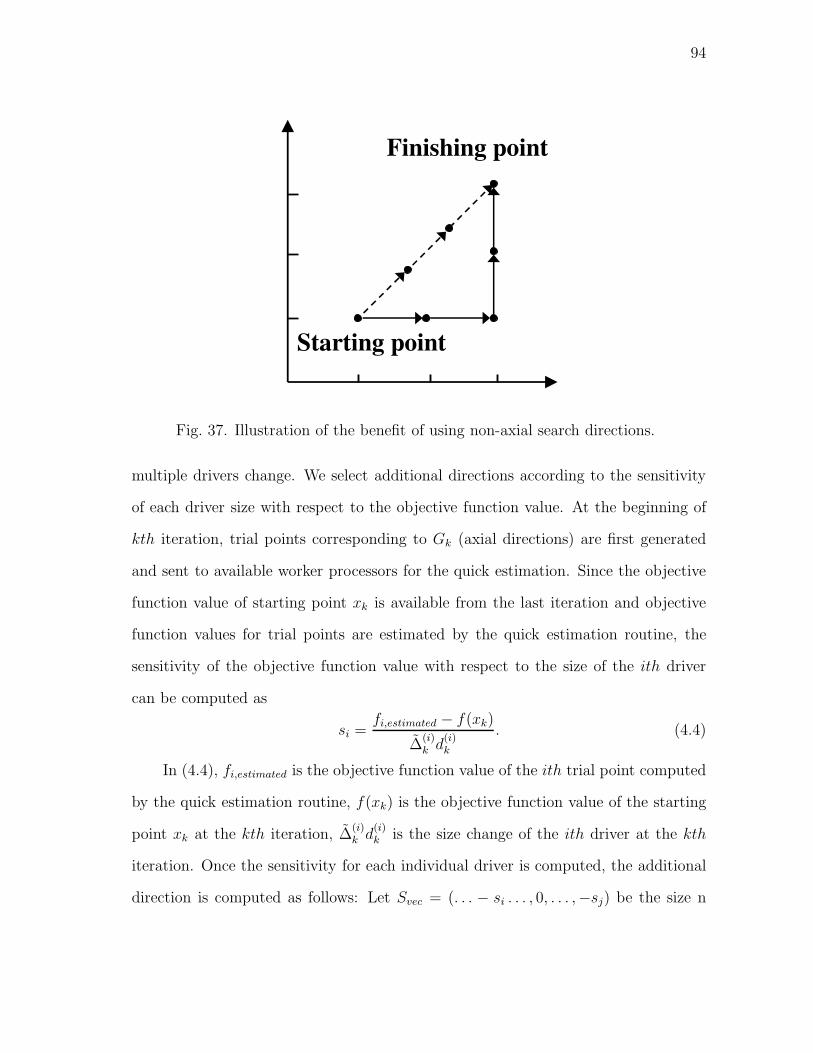
94

Starting point

Finishing point

Fig. 37. Illustration of the benefit of using non-axial search directions.

multiple drivers change. We select additional directions according to the sensitivity

of each driver size with respect to the objective function value. At the beginning of

kth iteration, trial points corresponding to Gk (axial directions) are first generated

and sent to available worker processors for the quick estimation. Since the objective

function value of starting point xk is available from the last iteration and objective

function values for trial points are estimated by the quick estimation routine, the

sensitivity of the objective function value with respect to the size of the ith driver

can be computed as

si =fi,estimated − f(xk)

∆(i)k d

(i)k

. (4.4)

In (4.4), fi,estimated is the objective function value of the ith trial point computed

by the quick estimation routine, f(xk) is the objective function value of the starting

point xk at the kth iteration, ∆(i)k d

(i)k is the size change of the ith driver at the kth

iteration. Once the sensitivity for each individual driver is computed, the additional

direction is computed as follows: Let Svec = (. . . − si . . . , 0, . . . ,−sj) be the size n

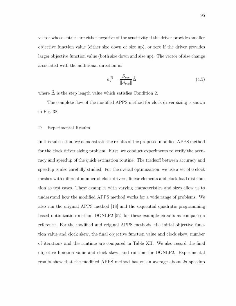
95

vector whose entries are either negative of the sensitivity if the driver provides smaller

objective function value (either size down or size up), or zero if the driver provides

larger objective function value (both size down and size up). The vector of size change

associated with the additional direction is:

h(l)k =

Svec

‖Svec‖∆ (4.5)

where ∆ is the step length value which satisfies Condition 2.

The complete flow of the modified APPS method for clock driver sizing is shown

in Fig. 38.

D. Experimental Results

In this subsection, we demonstrate the results of the proposed modified APPS method

for the clock driver sizing problem. First, we conduct experiments to verify the accu-

racy and speedup of the quick estimation routine. The tradeoff between accuracy and

speedup is also carefully studied. For the overall optimization, we use a set of 6 clock

meshes with different number of clock drivers, linear elements and clock load distribu-

tion as test cases. These examples with varying characteristics and sizes allow us to

understand how the modified APPS method works for a wide range of problems. We

also run the original APPS method [18] and the sequential quadratic programming

based optimization method DONLP2 [52] for these example circuits as comparison

reference. For the modified and original APPS methods, the initial objective func-

tion value and clock skew, the final objective function value and clock skew, number

of iterations and the runtime are compared in Table XII. We also record the final

objective function value and clock skew, and runtime for DONLP2. Experimental

results show that the modified APPS method has on an average about 2x speedup

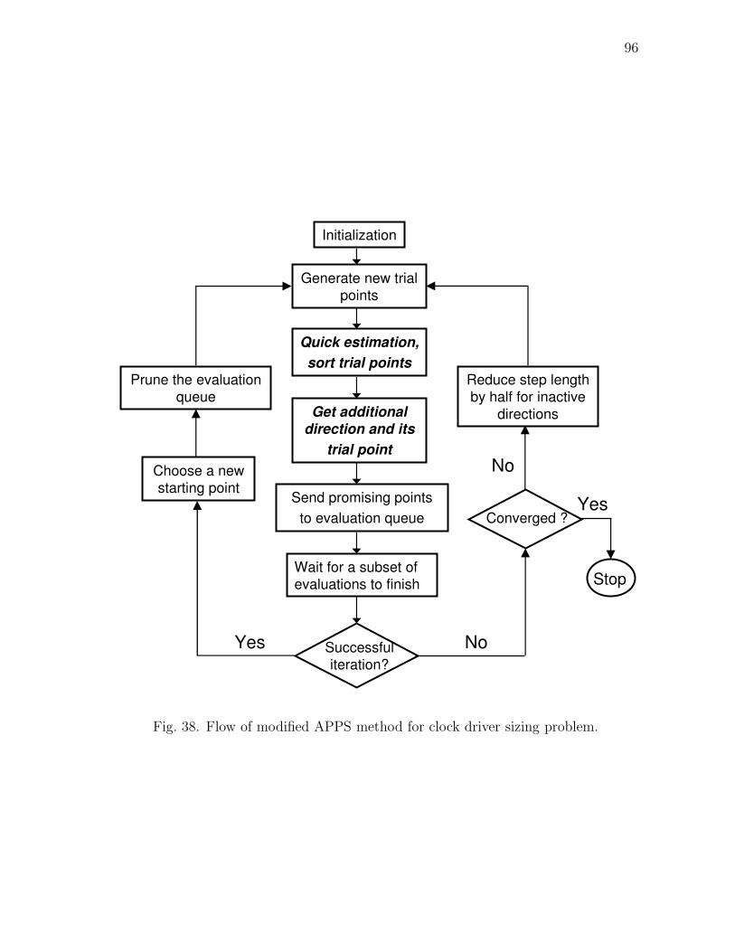
96

Initialization

Generate new trial

points

Wait for a subset of

evaluations to finish

Choose a new

starting point

Prune the evaluation

queue

Yes

Reduce step length

by half for inactive

directions

No

No

Stop

Yes

Successful

iteration?

Converged ?

Quick estimation,

sort trial points

Get additional

direction and its

trial point

Send promising points

to evaluation queue

Fig. 38. Flow of modified APPS method for clock driver sizing problem.

97

over the original APPS method while DONLP2 only works for very small test cases.

The driver merging step in the quick estimation routine is implemented using the Perl

scripting language. The model order reduction and transient circuit simulation pro-

gram is implemented in C++. The software package of the original APPS method is

freely available. We add the quick estimation and additional directions modifications

to the original APPS implementation. All experiments are conducted on a Linux

server with 8GB memory and two 2.33GHz quad-core processors. We use 7 proces-

sors for the original and modified APPS methods. 1 processor is the manager and 6

other processors are the workers.

The quick estimation routine needs to provide a fairly accurate estimation of the

objective function value for a trial point in much shorter time compared with the

full evaluation. The results of verifying the quick estimation routine are included in

Table X. We do both the quick estimation and full evaluation for three clock mesh

examples. Their corresponding runtimes, speedup of the quick estimation routine,

error of the quick estimation in objective function value are included. We can see that

for all three clock mesh examples, quick estimation routine achieves good accuracy

in objective function value in much shorter time compared with the full simulation.

In this way, it helps the modified APPS method to identify potentially successful

trial points before the full evaluations and provides estimated sensitivities which are

needed to decide the additional direction.

There is a tradeoff between the accuracy and runtime in the quick estimation

routine. In Table XI, we do the quick estimation for the same three clock mesh

examples. But we keep more drivers after the driver merging step. We can see that

the runtime of quick estimation is increased while the accuracy becomes better.

Next, we present the results of applying the original APPS method, our modified

APPS method and DONLP2 to the clock driver sizing problem. For every clock mesh

98

Table X. Verification of the quick estimation routine on three clock mesh examplesCkt # drivers # drivers # linear elements Runtime Runtime Speedup Error in objective

after merging full simu.(s) quick est.(s) function valuemesh1 15 5 2370 7.37 0.95 7.76 4.75%mesh2 20 5 16k 160.23 2.92 54.87 4.89%mesh3 25 5 25k 292.56 3.11 94.07 10.68%

Table XI. Tradeoff of quick estimation routine: more accuracy and less speedupCkt # drivers # drivers # linear elements Runtime Runtime Speedup Error in objective

after merging full simu.(s) quick est.(s) function valuemesh1 15 8 2370 7.37 1.93 3.82 3.17%mesh2 20 10 16k 160.23 8.05 19.90 0.98%mesh3 25 13 25k 292.56 19.95 14.66 4.52%

Table XII. Comparison between the original APPS method and the modified APPS

method on seven clock mesh examples# # linear Initial Initial Final Final Runtime Runtime Iterations Iterations

Ckt drivers elements function clock function clock original modified Speedup original modifiedvalue skew(ps) value skew(ps) APPS APPS APPS APPS

mesh1 15 2370 1.16e1 12.91 3.18e-1 2.82 6 mins 3 mins 2 48 35mesh2 20 16k 8.52e2 91.82 1.95 7.5 9 hrs 8 hrs 1.125 166 119mesh3 25 25k 7.02e2 100.98 1.57e1 21.7 25.75 hrs 11 hrs 2.34 225 76mesh4 25 27k 1.68e3 159.74 1.62e2 59.8 10.5 hrs 5.5 hrs 1.91 84 34mesh5 30 30k 5.07e2 103.88 4.30e1 38.6 27.5 hrs 12.5 hrs 2.2 158 62mesh6 50 40k 1.07e3 114.97 1.21e2 44 41 hrs 20 hrs 2.05 164 37

99

example, we start the three optimization methods with the same initial condition.

Original APPS method and modified APPS method use the same initial step length

and stopping criteria.

In Table XIII, we include the results of applying DONLP2 for the optimiza-

tion. We run DONLP2 for much longer time than APPS method for every example.

DONLP2 only reduces the objective function value for the smallest clock mesh. For all

the other larger ones, it does not effectively reduce the objective function value within

the time frame. The reason for the poor performance of DONLP2 is that DONLP2

needs to approximate the Hessian matrix of the Lagrangian internally, which requires

O(n2) full simulations of the clock mesh where n is the number of variables. For the

clock driver sizing problem where n is in the range of 20 to 50 and one simulation

takes a few minutes at least, approximating the Hessian matrix could take days.

Table XIII. Results of applying DONLP2 on the same set of clock mesh examples as

in Table XIIRuntime Initial Initial Final Final

Ckt DONLP2 function clock function clockvalue skew (ps) value skew (ps)

mesh1 20 hrs 1.16e1 12.91 6.04 9.83mesh2 47 hrs 8.52e2 91.82 8.49e2 90.78mesh3 48 hrs 7.02e2 100.98 7.01e2 100.95mesh4 48 hrs 1.68e3 159.74 1.68e3 159.72mesh5 58 hrs 5.07e2 103.88 5.07e2 103.84mesh6 58 hrs 1.07e3 114.97 1.07e3 114.96

Table XII summarizes the runtime and the number of iterations spent by the

original APPS method and the modified APPS method to reach the same objective

function value. For mesh1 and mesh2, the optimization process is carried to the

convergence. For all the other larger clock mesh examples, we stop the optimization

when it reaches a satisfying objective function value and clock skew. This is due to

practical considerations. At the later stages of the optimization, the APPS method

needs to spend much more time to find a successful trial point than it does in the

100

earlier stages. If the objective function value is already good enough, it would be

better to stop the optimization than continuing the optimization for a much longer

time to get a small improvement in objective function value. The modified APPS

method gets 2x speedup over the original APPS method on average. Also the modified

APPS method uses less number of iterations. The performance improvement is due

to the incorporation of the quick estimation step and additional directions.

From this comparison we can see that for this practical optimization problem

which is characterized by expensive objective function value evaluation and lack of

explicit derivative information, parallel pattern search based methods are much more

effective than sequential quadratic programming based method.

In Figs. 39 and 40, we show the relative clock arrival time distribution for a

clock mesh with smooth load distribution before and after the optimization. Here the

relative clock arrival time at each sink node is defined as Tj−µ, where Tj is the actual

clock arrival time at node j, µ is the average clock arrival time among all sink nodes.

We can see that after the clock driver size optimization, the clock arrival time at sink

nodes across the chip become much closer. In Figs. 41 and 42, we show the relative

clock arrival time distribution for a clock mesh with nonuniform load distribution

before and after the optimization. Again, after the optimization, the clock arrival

time across the chip become much closer.

E. Summary

In this chapter, we present a modified asynchronous parallel pattern search based

method for the clock mesh driver size optimization. The proposed method achieves

desirable results in terms of clock skew reduction and runtime. We believe this op-

timization method can be applied to other problems such as parameter tuning for

101

-6.00E-11

-4.00E-11

-2.00E-11

0.00E+00

2.00E-11

4.00E-11

6.00E-11

8.00E-11

1.00E-10

8.00E-11-1.00E-10

6.00E-11-8.00E-11

4.00E-11-6.00E-11

2.00E-11-4.00E-11

0.00E+00-2.00E-11

-2.00E-11-0.00E+00

-4.00E-11--2.00E-11

-6.00E-11--4.00E-11

Before optimization, smooth load distributionR

ela

tive c

lock

arr

ival

tim

e (

s)

Fig. 39. Clock arrival time distribution before optimization for smooth load distribu-

tion.

analog circuits.

102

-6.00E-11

-4.00E-11

-2.00E-11

0.00E+00

2.00E-11

4.00E-11

6.00E-11

8.00E-11

1.00E-10

8.00E-11-1.00E-10

6.00E-11-8.00E-11

4.00E-11-6.00E-11

2.00E-11-4.00E-11

0.00E+00-2.00E-11

-2.00E-11-0.00E+00

-4.00E-11--2.00E-11

-6.00E-11--4.00E-11

After optimization, smooth load distributionR

ela

tive c

lock

arr

ival

tim

e (

s)

Fig. 40. Clock arrival time distribution after optimization for smooth load distribution.

-1.50E-10

-1.00E-10

-5.00E-11

0.00E+00

5.00E-11

1.00E-10

1.50E-10

1.00E-10-1.50E-10

5.00E-11-1.00E-10

0.00E+00-5.00E-11

-5.00E-11-0.00E+00

-1.00E-10--5.00E-11

-1.50E-10--1.00E-10

Before optimization, non-uniform load distribution

Rela

tive c

lock

arr

ival

tim

e (

s)

Fig. 41. Clock arrival time distribution before optimization for non-uniform load dis-

tribution.

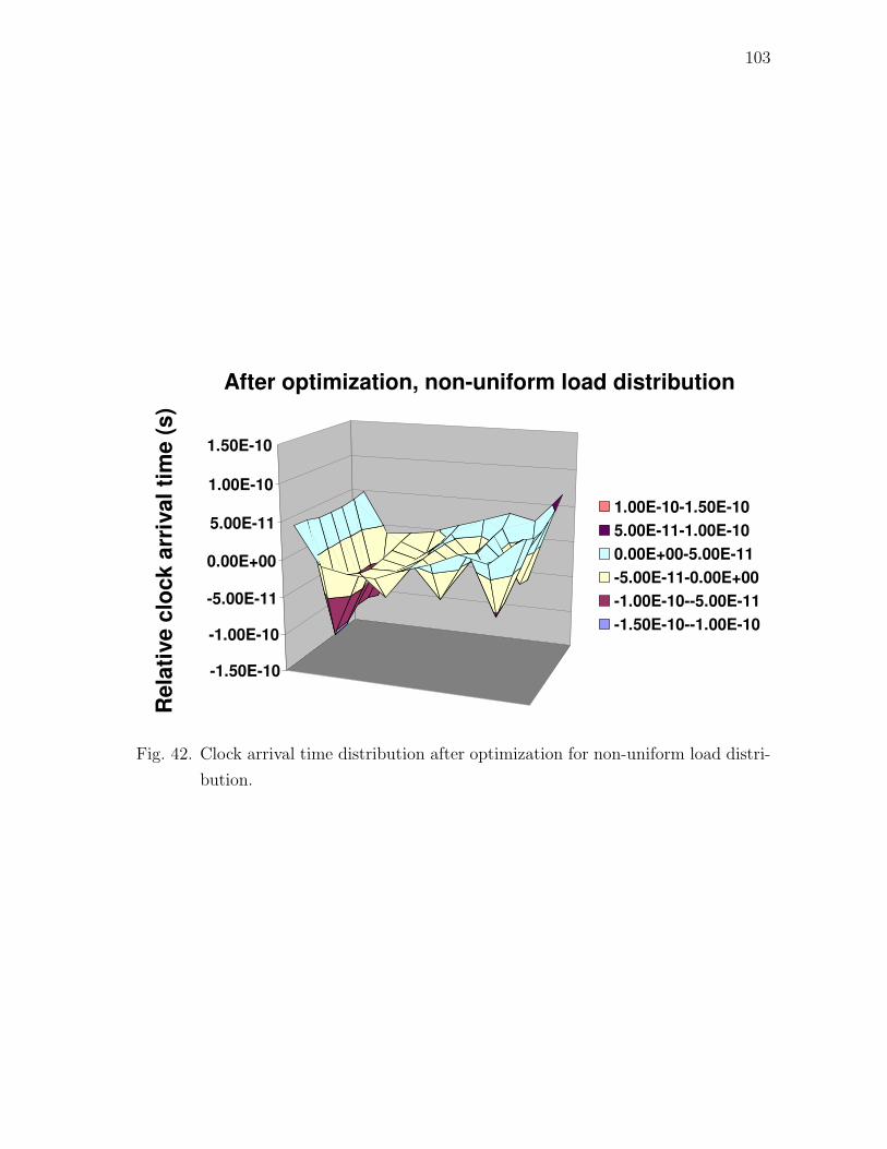
103

-1.50E-10

-1.00E-10

-5.00E-11

0.00E+00

5.00E-11

1.00E-10

1.50E-10

1.00E-10-1.50E-10

5.00E-11-1.00E-10

0.00E+00-5.00E-11

-5.00E-11-0.00E+00

-1.00E-10--5.00E-11

-1.50E-10--1.00E-10

After optimization, non-uniform load distribution

Rela

tive c

lock

arr

ival

tim

e (

s)

Fig. 42. Clock arrival time distribution after optimization for non-uniform load distri-

bution.

104

CHAPTER V

PARALLEL PERFORMANCE MODELING AND OPTIMIZATION

With the increasing popularity of multi-core processors and the promise of future

many-core systems, parallel CAD algorithm development has attracted a significant

amount of research effort. However, a highly relevant issue, parallel program perfor-

mance modeling has received little attention in the EDA community. Performance

modeling serves the critical role of guiding parallel algorithm design and provides a

basis for runtime performance optimization. In subsection A, we propose a system-

atic composable approach for the performance modeling of the hierarchical multi-

algorithm parallel circuit simulation (HMAPS) approach. The unique integration

of inter- and intra-algorithm parallelism allows a multiplicity of parallelism to be

exploited in HMAPS and also creates interesting modeling challenges in forms of

complex performance tradeoffs and large runtime configuration space. We model the

performance of key subtask entities as functions of workload and parallelism. We ad-

dress significant complications introduced by inter-algorithm interactions in terms of

memory contention and collaborative simulation behavior via novel penalty and sta-

tistical based modeling. In subsection B, we propose a runtime optimization approach

that allows for automatic on-the-fly reconfiguration of the parallel simulation code.

We show how the runtime information, collected as parallel simulation proceeds, can

be combined with the static parallel performance models to enable dynamic adapta-

tion of parallel simulation execution for improved runtime and robustness.

A. Performance Modeling of HMAPS

Since the hierarchical multi-algorithm parallel circuit simulation (HMAPS) approach

uses a combination of inter- and intra-algorithm parallel techniques, HMAPS can

105

choose from a variety of different configurations. More specifically, there are four

simulation algorithms to be chosen in HMAPS, each algorithm can use 0 or 1 or 2

or 4 cores, therefore, the total number of HMAPS configurations is 44 − 1 = 255.

Since different algorithms have different stepsizes, convergence properties, etc and

some algorithms may use cores more efficiently, the runtime of different HMAPS

configurations can be vastly different. In our experiments, we have observed that

a configuration with good combination of algorithms and core assignment can be

9x faster than a configuration with bad combination of algorithms and core assign-

ment. Without the performance modeling of HMAPS, the selection of configuration

is entirely based on prior experience.

1. Overview

The objectives of the performance modeling of HMAPS are two fold:

• We want to use the performance model to predict the runtime of HMAPS over

the large configuration space

• The performance modeling provides the basis for the adaptive configuration

selection in HMAPS during the runtime

In order to achieve these two objectives, several things need to be modeled. First

of all, we need to model the runtime of an individual algorithm which is the building

block of HMAPS. Second, we need to model the memory condition of the computing

platform. Third, the inter-algorithm collaboration in HMAPS has to be modeled.

To model the runtime of an individual algorithm, our strategy is to decompose the

simulation algorithm into four interrelated components: matrix solve, device evalua-

tion, nonlinear iteration and numerical integration. Nonlinear iteration is performed

at every time step to solve a set of nonlinear circuit equations. Within each nonlinear

106

iteration, one matrix solve and one model evaluation of all devices are performed.

After the convergence of the nonlinear iteration, numerical integration method com-

putes the stepsize ∆t for the next time point. We build the component-level model

for each of them. The composable approach is illustrated in Fig. 43.

Device

evaluation

Matrix

solve

T=T+∆t

Converged?

Algorithm-1

Algorithm-2

Algorithm-3

Algorithm-4

Core 1

Core 2

Core 3

Core 4

Core 5

Core 6

Core 7

Core 8

Shared

memory

Nonlinear

iteration

Numerical

integration

Memory

bus

Fig. 43. Illustration of modeling tasks.

Based on the above decomposition, the runtime of a simulation algorithm can

be computed as:

Runtime =Tsim

∆taverage

[N · (T (matrix) + T (device))], (5.1)

where Tsim is the total simulation time, ∆taverage is the average stepsize, N is the

average number of iterations at every time step, T (matrix) is the time spent on one

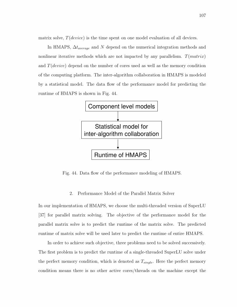
107

matrix solve, T (device) is the time spent on one model evaluation of all devices.

In HMAPS, ∆taverage and N depend on the numerical integration methods and

nonlinear iterative methods which are not impacted by any parallelism. T (matrix)

and T (device) depend on the number of cores used as well as the memory condition

of the computing platform. The inter-algorithm collaboration in HMAPS is modeled

by a statistical model. The data flow of the performance model for predicting the

runtime of HMAPS is shown in Fig. 44.

Component level models

Statistical model for

inter-algorithm collaboration

Runtime of HMAPS

Fig. 44. Data flow of the performance modeling of HMAPS.

2. Performance Model of the Parallel Matrix Solver

In our implementation of HMAPS, we choose the multi-threaded version of SuperLU

[37] for parallel matrix solving. The objective of the performance model for the

parallel matrix solve is to predict the runtime of the matrix solve. The predicted

runtime of matrix solve will be used later to predict the runtime of entire HMAPS.

In order to achieve such objective, three problems need to be solved successively.

The first problem is to predict the runtime of a single-threaded SuperLU solve under

the perfect memory condition, which is denoted as Tsingle. Here the perfect memory

condition means there is no other active cores/threads on the machine except the

108

core/thread used by SuperLU. Therefore, there is no memory contention of any kind.

That one core/thread used by SuperLU can have all the memory bandwidth and stor-

age. The second problem is to predict the speedup of SuperLU with different number

of cores/threads under the prefect memory condition, which is denoted as Sp(n), here

n is the number of threads used by SuperLU. Again, there is no active core/thread

on the machine except the cores/threads used by SuperLU. The third problem is to

predict the performance degradation factor of SuperLU under the imperfect memory

condition where there are other active cores/threads running on the machine at the

same time. The performance degradation factor is denoted as fp. If all three problems

are solved, the runtime of SuperLU under an HMAPS configuration can be computed

as

T (matrix) = Tsingle · Sp(n) · fp. (5.2)

Notice that different HMAPS configurations may cause different memory conditions

due to their distinct algorithm combinations and core assignments. Therefore, fp is

changing with the HMAPS configurations.

From our measurement data, we found that Tsingle is largely impacted by the

number of non-zeros in the LU factors of the matrix. However, it is impossible to know

the number of non-zeros in the LU factors without factorizing the matrix. Although

it is possible to write a symbolic factorization routine with the column preordering

algorithm which only computes the number of non-zeros in the LU factors, such

effort may derail the purpose of modeling and fast prediction of matrix solve time

from a SuperLU user’s point of view. Therefore, we decide that for a given circuit,

we perform a one time matrix solve to measure Tsingle.

To predict Sp(n), one has to understand how SuperLU works. In [37], a posteriori

performance model for estimating the optimal speedup of SuperLU is presented. That

109

performance model depends on the a lot of internal procedures of SuperLU such as

the updating sequence of the nodes, the partition of the matrix, etc. Therefore, it is

hard to build a performance model which only depends on a few parameters of the

matrix and still gives good prediction for speedup since many important factors about

the SuperLU solver are not considered. Given these facts, we decide that instead of

predicting Sp(n), we perform the matrix solve with different number of cores to get

Sp(n) upfront. Since each algorithm in HMAPS uses up to 4 cores to do parallel

matrix solve, only three additional matrix solve and measurement are needed to get

the Sp(n) for all the possible 255 HMAPS configurations. However, predicting Sp(n)

from a parallel matrix user’s perspective may be an interesting future research topic.

Then the last problem remaining is to predict the performance degradation factor

fp of SuperLU under various HMAPS configurations. In order to build a performance

model for fp, we have to understand what parameters can be used to quantitatively

describe the memory condition. From our measurement data, we observed that the

runtime of SuperLU is increasing with the number of additional active threads on

the machine. This is understandable since more active threads will generate more

memory traffic, therefore, the increased contention on the memory bus will decrease

the memory bandwidth of each thread. The decreased memory bandwidth of each

thread causes the slowdown of the solver. However, active threads influence the matrix

solver differently. For example, if an active thread seldom accesses the memory, it

would not cause any noticeable contention on the memory. If it does access memory

very often, it will cause higher memory contention and smaller memory bandwidth

for each thread on the machine.

Based on these observations, we propose a simple quantitative model for the

memory condition: for one additional active thread on the machine, there is a penalty

term p associated with this thread. This p is an abstract parameter which represents

110

the aggregated effect of that active thread on the overall memory condition of the

machine. Different active threads may have different penalties due to their distinct

memory access pattern. The penalty is additive. The total penalty P of all other

active threads is computed as

P =∑

i

(pi × ni), (5.3)

where pi is the per-thread penalty from the ith algorithm in HMAPS, ni is the number

of threads used in the ith algorithm in HMAPS. Fig. 45 demonstrates how the runtime

of matrix solve is changing with the penalty. We can see that under the worst memory

condition (largest penalty), the runtime of matrix solve can be 2x of the runtime under

perfect memory condition.

Another circuit-dependent factor for fp is the number of non-zeros in the LU

factors. Since SuperLU uses compressed form to store matrices, a bunch of non-

zeros can be fetched at the same time, therefore, the cost of data communication

is not proportionally increasing with the number of non-zeros in the LU factors.

However, the computational cost is still proportional to the number of non-zeros

in the LU factors. Therefore, the portion of the communication cost in the total

matrix solve time becomes smaller as the number of non-zeros in the LU factors

increase. While the data communication is impacted by the memory condition, the

data computation is not. This is why as the number of non-zeros in the LU factors

increases, the performance degradation factor fp is increasing more slowly with the

memory condition degradation. Fig. 46 demonstrates such characteristic. X-axis is

the index for a set of HMAPS configurations with increasing number of threads/cores

on the machine, which represents the gradually degraded memory condition. For the

same set of HMAPS configurations, fp is increasing more slowly for matrix with larger

number of non-zeros in the LU factors.

111

0 0.1 0.2 0.3 0.40.02

0.03

0.04

0.05

Penalty

Run

time

of m

atrix

sol

ve

Fig. 45. Runtime of matrix solve is increasing with the penalty from other active

threads.

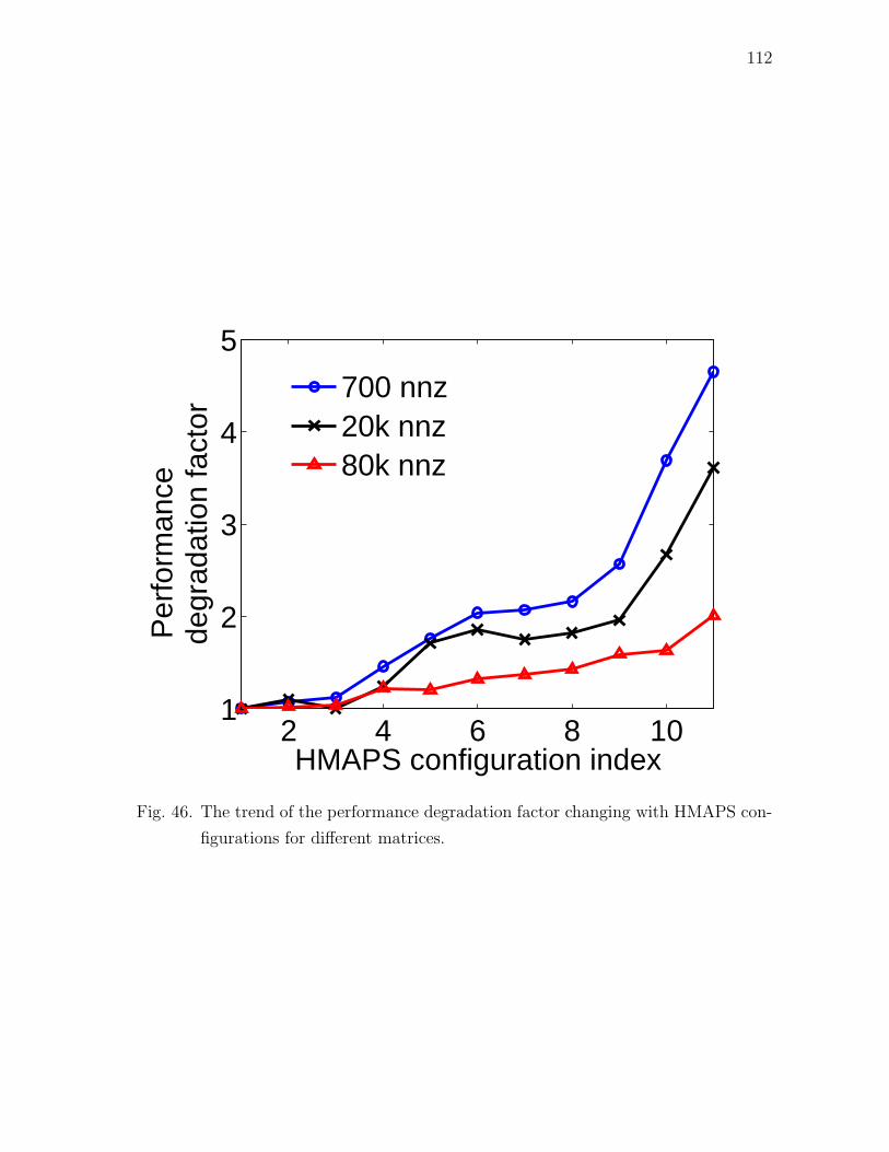
112

2 4 6 8 101

2

3

4

5

HMAPS configuration index

Per

form

ance

de

grad

atio

n fa

ctor

700 nnz20k nnz80k nnz

Fig. 46. The trend of the performance degradation factor changing with HMAPS con-

figurations for different matrices.

113

After we decide on the parameters that are important to fp, we perform extensive

pre-characterization of matrix solve on different matrices to build the lookup table

(LUT) for fp. The lookup table has four input parameters: the number of threads

used by matrix solver, the number of non-zeros in the LU factors, the total penalty

P computed by (5.3) and the total number of active threads on the machine. Usually

only the first three parameters are needed to locate an entry in the LUT. Then

interpolation can be used to compute fp for an HMAPS configuration. But it is

possible that for two HMAPS configurations in the LUT, the first three parameters

are the same, but they have different fps. In this case, we need the 4th parameter

which is the total number of threads to further distinguish them. Obviously we want

to cover a wide range of matrices in the lookup table. For the total penalty P , we

do not exhaustively sample all the possible HMAPS configurations. We only select

a few sample points which cover the entire range of penalty. The four-dimensional

lookup table is illustrated in Fig. 47.

Penalty

# of threads

in solver

# of threads

on system

# of non-zeros in LU factors

……Data

for fp

Fig. 47. Four-dimensional lookup table for the parallel matrix solver.

Below is the procedure of predicting the runtime of matrix solve for a new circuit

under an HMAPS configuration:

1. Do circuit-specific measurement to get Tsingle and Sp(n).

114

2. Interpolate to get pi for the current circuit from pre-characterized data of cir-

cuits with similar non-zero pattern in the LU factors of the system matrices.

3. Compute the total penalty P using (5.3) for the current configuration.

4. Use the number of threads used in SuperLU n, number of non-zeros in the LU

factors and P as inputs to locate entries in the pre-characterized lookup table

of fp.

5. Use interpolation to predict the performance degradation factor fp under such

HMAPS configuration.

6. Use the total number of threads to interpolate for fp if necessary.

7. Calculate Tsingle ·Sp(n) ·fp to get T (matrix) under such HMAPS configuration.

Notice that step 1 and 2 do not need to be repeated for the same circuit under

different HMAPS configurations. Step 3− 7 can be performed rather efficiently for a

new HMAPS configuration.

The performance modeling of the parallel device evaluation, matrix resolve rou-

tine in successive chord method are done in the similar fashion. The only difference

is that we do not perform any circuit-specific measurement like we did for Tsingle

and Sp(n) in parallel matrix solve modeling. We build the multi-dimensional lookup

table for the runtime and get the T (device) directly from the lookup table. Notice

that our performance models are built for a specific computing platform since our

measurements are performed on one platform. If we migrate HMAPS onto a different

platform, we need to rebuild all the lookup tables.

115

1 2 3 4 50

200

400

600

Number of Iterations

Fre

quen

cy

(a)

0 5 10 150

20

40

60

80

Number of Iterations

Fre

quen

cy

(b)

Fig. 48. (a)Number of iterations distribution for BE method. (b)Number of iterations

distribution for Dassl method.

3. Performance Modeling of Nonlinear Iterative Methods and Numerical

Integration Methods

We use discrete random variable to model the number of iterations of a simula-

tion algorithm since the iteration counts can only take discrete values. Fig. 48(a)

shows the distribution of iteration counts for the simulation algorithm: Newton+BE.

Fig. 48(b) shows the distribution of the iteration counts for the simulation algorithm:

Newton+Dassl. Newton+Dassl has larger iteration counts due to the larger stepsize

produced by Dassl.

For the same type of circuits, one simulation algorithm usually has similar dis-

tributions of iteration counts. In our model, we run each simulation algorithm for

different types of circuits. For the same type of circuits, we do profiling for each

simulation run to get the distribution of iteration counts. After we simulate suffi-

cient number of circuits within the same type, we compute the average of all profiled

distributions as the distribution of iteration counts for that type of circuits. The aver-

aged distribution is represented by a discrete random variable. Since successive chord

116

method is not robust as a stand-alone simulation algorithm, if it fails to converge at

some points during the simulation, we assign a large number (e.g. 1000) to the itera-

tion count. The probability associated with that large number is determined by the

probability of convergence failure of successive chord method. We have a distribution

of iteration counts for each of the four simulation algorithms for every circuit type.

The handling of numerical integration method is simpler. In (5.1), only the aver-

age stepsize ∆taverage is important. Therefore, we take the similar profiling approach

as we did for nonlinear iterative methods to characterize the average stepsize. After

the characterization, we will have an average stepsize for each simulation algorithm

for every circuit type.

4. Performance Modeling of Inter-Algorithm Collaboration

After the component level models for each of the four components are built, we are

now ready to model the inter-algorithm interaction of HMAPS. For each simulation

algorithm within an HMAPS configuration, the runtime of one iteration can be com-

puted as:

T (matrix) + T (device), (5.4)

where T (matrix) and T (device) are the runtime for one matrix solve and one model

evaluation of all devices. They are predicted by the component level models in sub-

section 2.

We use Di to denote the distribution of iteration counts , ∆taverage i to denote the

average stepsize for the ith simulation algorithm in HMAPS. Both of them are ob-

tained from the component level models described in subsection 3. Then the runtime-

per-unit simulation time for the the ith simulation algorithm (Tunit i) can be computed

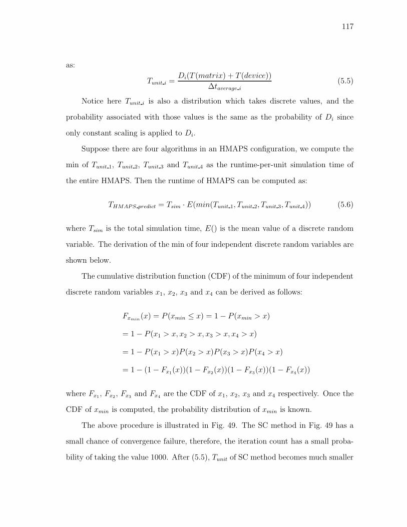
117

as:

Tunit i =Di(T (matrix) + T (device))

∆taverage i

(5.5)

Notice here Tunit i is also a distribution which takes discrete values, and the

probability associated with those values is the same as the probability of Di since

only constant scaling is applied to Di.

Suppose there are four algorithms in an HMAPS configuration, we compute the

min of Tunit 1, Tunit 2, Tunit 3 and Tunit 4 as the runtime-per-unit simulation time of

the entire HMAPS. Then the runtime of HMAPS can be computed as:

THMAPS predict = Tsim · E(min(Tunit 1, Tunit 2, Tunit 3, Tunit 4)) (5.6)

where Tsim is the total simulation time, E() is the mean value of a discrete random

variable. The derivation of the min of four independent discrete random variables are

shown below.

The cumulative distribution function (CDF) of the minimum of four independent

discrete random variables x1, x2, x3 and x4 can be derived as follows:

Fxmin(x) = P (xmin ≤ x) = 1− P (xmin > x)

= 1− P (x1 > x, x2 > x, x3 > x, x4 > x)

= 1− P (x1 > x)P (x2 > x)P (x3 > x)P (x4 > x)

= 1− (1− Fx1(x))(1− Fx2

(x))(1− Fx3(x))(1− Fx4

(x))

where Fx1, Fx2

, Fx3and Fx4

are the CDF of x1, x2, x3 and x4 respectively. Once the

CDF of xmin is computed, the probability distribution of xmin is known.

The above procedure is illustrated in Fig. 49. The SC method in Fig. 49 has a

small chance of convergence failure, therefore, the iteration count has a small proba-

bility of taking the value 1000. After (5.5), Tunit of SC method becomes much smaller

118

than Tunit of Newton+BE method since the runtime-per-iteration of SC method is

much smaller. However, there is still a faraway value for Tunit of SC which corresponds

to the case of convergence failure. After taking the min of the two discrete random

variables, that faraway value is filtered out. This is consistent with the inter-algorithm

collaboration in HMAPS where robust algorithm can help non-robust algorithm jump

out of its non-convergence area.

1 2 3 4 5 1 2 3 41000

Distribution of iteration

counts for SC

Distribution of iteration

counts for Newton+BE

Multiplied with runtime-per-iteration,

then divided by average stepsize

Min of two discrete random variables

Runtime-per-unit time

for both algorithms

Runtime-per-unit time

for HMAPS

……

Fig. 49. Illustration of the statistical model.


In this subsection, we demonstrate the accuracy of the component level models and

the performance model of HMAPS. Our implementation of HMAPS can choose four

119

simulation algorithms: Newton+Backward Euler, Newton+Gear2, Newton+Dassl,

Successive chord+ Dynamic timestep rounding. Each simulation algorithm in HMAPS

can use 1 or 2 or 4 cores to do the low-level parallel matrix solve and device eval-

uation. Since the machine on which we run HMAPS simulations only has 8 cores,

we do not use more than 8 threads in HMAPS. Therefore, there is no contention on

the cores. All the parallel implementations are done using Pthread APIs which are

especially suitable for the shared memory machine that we use.

First, we demonstrate the accuracy of the component level model for parallel

matrix solve described in subsection 2. The first test circuit is a combinational circuit

with 1200 transistors and 600 linear elements. We predict the matrix solve time for

its system matrix for 100 HMAPS configurations. Then we run HMAPS with these

100 different configurations and measure the actual matrix solve time. The actual

matrix solve time can vary up to 2x across different HMAPS configurations. The

relative errors of these 100 predicted matrix solve time are shown in Fig. 50(a). We

can see that the relative errors are within −10% ∼ 10%.

−0.1 −0.05 0 0.05 0.10

5

10

15

20

25

Relative error

Fre

quen

cy

(a)

−0.2 −0.1 0 0.10

5

10

15

20

25

Relative error

Fre

quen

cy

(b)

Fig. 50. (a)Relative error of the predicted matrix solve time for a matrix. (b)Relative

error of the predicted matrix solve time for a larger matrix.

120

The second test circuit is a combinational circuit with 2000 transistors and 1000

linear elements. The experimental procedure is similar to the previous example. The

relative error of 100 predicted matrix solve time are shown in Fig. 50(b). Again, most

of the errors are within −10% ∼ 10%.

Now, we demonstrate the validity and accuracy of the performance model of the

entire HMAPS. We use four circuits with different sizes and structures as test circuits.

The first circuit is a transistor dominant combinational circuit with 1000 transistors

and 500 linear elements. The second circuit is also a combinational circuit with 2200

transistors and 1100 linear elements. The third circuit is a clock mesh circuit with 18k

linear elements and 20 clock drivers. The fourth circuit is a larger clock mesh circuit

with 28k linear elements and 25 clock drivers. These four circuits were not used in the

profiling for generation of component level models. The HMAPS configurations we

use in the performance prediction are shown in Table XIV. Table XIV is interpreted

in this way: in the first HMAPS configuration (the 1st row), there are two algorithms:

Newton+BE and successive chord. Newton+BE uses 1 core and successive chord uses

4 cores. “− /−′′ for Newton+Gear2 and Newton+Dassl means they are not used in

this configuration. We can see that Newton+BE is always used because it serves as

a solid backup solution in case other simulation algorithms fail to converge. And it

never uses more than 1 core since we want to assign more cores to faster algorithms

to get larger speedup.

Table XIV. Algorithm composition for a set of HMAPS configurationsHMAPS Core allocationConfig Newton+BE SC Newton+Gear2 Newton+Dassl

1 1 4 -/- -/-2 1 2 -/- -/-3 1 1 -/- -/-4 1 -/- -/- 45 1 -/- 4 -/-6 1 4 2 -/-7 1 2 1 2

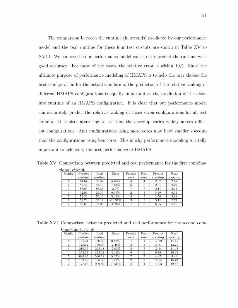
121

The comparison between the runtime (in seconds) predicted by our performance

model and the real runtime for these four test circuits are shown in Table XV to

XVIII. We can see the our performance model consistently predict the runtime with

good accuracy. For most of the cases, the relative error is within 10%. Since the

ultimate purpose of performance modeling of HMAPS is to help the user choose the

best configuration for the actual simulation, the prediction of the relative ranking of

different HMAPS configurations is equally important as the prediction of the abso-

lute runtime of an HMAPS configuration. It is clear that our performance model

can accurately predict the relative ranking of those seven configurations for all test

circuits. It is also interesting to see that the speedup varies widely across differ-

ent configurations. And configurations using more cores may have smaller speedup

than the configurations using less cores. This is why performance modeling is vitally

important to achieving the best performance of HMAPS.

Table XV. Comparison between predicted and real performance for the first combina-

tional circuitConfig Predict Real Error Predict Real Predict Real

runtime runtime rank rank speedup speedup1 64.67 69.57 -7.04% 4 4 2.87 2.672 80.44 83.46 -3.62% 6 6 2.31 2.223 88.09 86.36 2.0% 7 7 2.11 2.154 32.05 29.30 9.39% 2 1 5.79 6.335 74.36 70.49 5.49% 5 5 2.50 2.636 59.76 67.12 -10.97% 3 3 3.11 2.777 30.66 31.05 -1.26% 1 2 6.05 5.98

Table XVI. Comparison between predicted and real performance for the second com-

binational circuitConfig Predict Real Error Predict Real Predict Real

runtime runtime rank rank speedup speedup1 151.34 150.30 0.69% 1 1 17.29 17.412 176.62 190.90 -7.48% 3 3 14.81 13.713 210.36 228.48 -7.93% 5 5 12.44 11.454 264.55 253.31 4.44% 6 6 9.89 10.335 620.05 590.12 5.07% 7 7 4.22 4.436 168.36 166.36 1.20% 2 2 15.54 15.737 177.68 209.89 -15.35% 4 4 14.73 12.47

122

Table XVII. Comparison between predicted and real performance for the first clock

mesh circuitConfig Predict Real Error Predict Real Predict Real

runtime runtime rank rank speedup speedup1 34.59 33.33 3.78% 1 1 20.56 21.342 51.09 51.04 1.0% 3 3 13.92 13.933 84.17 80.83 4.13% 5 5 8.45 8.804 116.76 123.03 -5.10% 6 6 6.09 5.785 300.25 297.31 0.99% 7 7 2.37 2.396 38.54 36.11 6.73% 2 2 18.45 19.697 68.40 58.05 17.83% 4 4 10.40 12.25

Table XVIII. Comparison between predicted and real performance for the second clock


runtime runtime rank rank speedup speedup1 111.15 106.76 4.11% 1 1 16.17 16.832 165.86 167.77 -1.14% 3 3 10.83 10.713 288.63 266.07 8.48% 5 5 6.23 6.754 351.96 340.21 3.45% 6 6 5.11 5.285 947.69 901.87 5.08% 7 7 1.90 1.996 129.50 118.06 9.69% 2 2 13.87 15.227 207.88 201.95 2.94% 4 4 8.64 8.90

We also show the histogram of the relative error distribution for the performance

modeling. We run 300 configurations for each circuit and plot the relative error

distribution histogram. We can see from Figs. 51 and 52 that the relative error of

our performance modeling scheme is still small over a large configuration space.

6. Summary

In this subsection, we present a systematic approach for the performance modeling

of a hierarchical multi-algorithm parallel circuit simulator. Our performance models

can accurately predict the runtime of the parallel circuit simulator. The performance

modeling work provides the basis for the future exploration of the dynamic runtime

optimization of the simulator.

123

−0.3 −0.2 −0.1 0 0.1 0.2 0.3 0.40

10

20

30

40

50

60

70

80

Relative error

Occ

uren

ce

Fig. 51. Histogram of the relative error for one circuit example.

B. Runtime Optimization for HMAPS

A static performance modeling for HMAPS has been reported in subsection A. How-

ever, static, or pre-runtime, parallel performance modeling has several limitations.

Static modeling is geared towards characterizing the parallel simulation performance

over a generic class of circuit types and sizes. In some sense, the resulted performance

models only capture average simulation performances. As such, these models are

not best descriptive for a given simulation instance. Furthermore, complex runtime

characteristics are not being captured and the opportunity of runtime performance

optimization is not exploited.

124

−0.2 −0.1 0 0.1 0.2 0.3 0.40

10

20

30

40

50

60

Relative error

Occ

uren

ce

Fig. 52. Histogram of the relative error for another circuit example.

In this subsection, we take one-step further to develop an on-the-fly runtime op-

timization approach for HMAPS. We dynamically adapt the HMAPS configuration

over a large configuration space for a given circuit being simulated, and based upon

valuable runtime information gathered as the simulation proceeds. We specifically

focus on several key runtime characteristics of multi-algorithm parallel simulation: 1)

characterization of convergences/strengths of multiple nonlinear iterative methods, 2)

characterization of time step sizes of multiple numerical integration methods, and 3)

automatic detection of convergence failure and algorithm deselection. The collection

and processing of the above dynamic information plays a significant role in selecting

125

the best subset of simulation algorithms to launch on-the-fly; it also provides a basis

to determine the optimal amount of parallelism (e.g. number of threads) that shall

be assigned to each active algorithm dynamically. On the other hand, these runtime

characteristics are complex functions of the circuit being simulated, and temporal

activities of the circuit experienced during the simulation. It is impossible to capture

such information in pre-runtime performance modeling. Our results have shown that

the proposed runtime approach not only finds the near-optimal code configuration

over a large configuration space, it also outperforms simple parallel code execution as

well as multi-algorithm simulation code assisted only with static performance model-

ing.

1. On-the-fly Automatic Adaptation

While pre-runtime parallel performance models capture the baseline performance

characteristics of each HMAPS configuration, they provide a basis for optimal configu-

ration selection at the onset of simulation. However, since crucial runtime simulation

performance data become available as the simulation proceeds, leveraging runtime

knowledge will lead to improved runtime efficiency and robustness. Runtime infor-

mation is particularly helpful for modeling performance characteristics that are highly

circuit dependent and temporally varying.

Fig. 53 illustrates the basic idea of the proposed on-the-fly automatic adaptation

of HMAPS. Reconfiguration of HMAPS takes place with a user-defined time granu-

larity, which defines how frequently the code is adapted. As the simulation proceeds,

several key parallel runtime performance data from the executed HMAPS configura-

tions in the past history are measured and stored as part of the simulation. To select

the best configuration for the next reconfiguration time, key runtime information is

extracted. Instead of completely discarding the existing pre-runtime performance

126

models, the extracted runtime information is properly processed and combined with

the pre-runtime data to generate an updated (”instantaneous”) set of parallel per-

formance models. The next best HMAPS configuration is predicted and selected

using the updated performance models. We will explain in the following subsections

how the dynamic runtime information is used to predict the HMAPS configuration

on-the-fly.

Config 1 Config 2Config N

Next Best Configuration ??

T i t

User defined configuration update granularity

Config 3

Predict next

Transient

simulation

time point

User-defined configuration update granularity Predict next

best configuration

Fig. 53. Dynamic reconfiguration for runtime optimization.

a. Dynamically Updated Step Size

It is understood that the average step size of a numerical integration method is a

strong function of circuit characteristics and temporal circuit activities. For example,

as more hard switchings are experienced in the simulation, an automatic time step

control algorithm will cut down the step size to ensure the simulation accuracy. Such

information is only available during runtime and can be exploited to provide improved

parallel performance prediction.

However, defining a general circuit activity metric, which works under all possible

127

circuit types and operations, is difficult. Instead, we collect the historical step size

information and extract circuit activity implicitly from the history. To this end, it is

meaningful to implement a ”fading” memory for predicting future step size based on

historical data. It entails assigning a larger weight to step sizes that are collected at

time instances closer to the prediction time. It is meaningful since the circuit state

tends to evolve continuously in time.

Next Best Configuration ??

Weights decay

exponentially in distance Next Best Configuration ??

Step size for numerical

integration?

Forgotten step sizes exponentially in distance

to the prediction time

Memory Window

Fig. 54. Fading memory: dynamic updating of step size.

Our scheme is illustrated in Fig. 54. As described in subsection A, the average

step size ∆taverage i of each numerical integration method is important in the perfor-

mance model. During the simulation, for each algorithm that is currently running, all

the historical information of its step size are saved. And they are used to predict the

step size that it will be used for the future. We enforce a time window for the step size

selection. If the step size information is too old (out of a certain time window), we

do not use it. We only use the historical step size information that is within a certain

time window to the current time point. For all the valid step sizes that are within

the time window, we compute their weighted average using the following equation:

∆history =

n∑

l=1

αl∆l, (5.7)

128

where ∆l is the step size at the lth time point, αl is the weight for ∆l. αl is computed

as:

αl = e−distancel

T (5.8)

where distancel is the distance between the current time point and the lth time point,

T is the size of the time window. We can see that the weight is decreasing as distancel

increases. This is consistent with the understanding of circuit simulation that more

recent time points are more important to the future time points. We also need to

consider the static step size that comes from the pre-characterized data. The overall

dynamic step size is computed as:

∆dynamic = α0∆static +

n∑

l=1

α′l∆l, (5.9)

where ∆static is the static step size given by the pre-characterized data, its weight α0

is empirically set to 0.1, α′l are normalized αl from equation (5.8). Then this ∆dynamic

will be used in equation (5.5) as ∆taverage i at the next configuration update point.

b. Dynamically Updated Iteration Count

The handling of historical information for the iteration count is similar to the step

size. But updating the iteration count is slightly different from updating the step size

since the iteration count is a distribution rather than a scalar value. We update the

mean value of the iteration count. For example, if we collected the iteration count

data at some sample time points, the updated iteration count distribution is:

Di,dynamic = Di + (meannew −E(Di)) (5.10)

where Di is the iteration count distribution from the pre-characterized data, meannew

is the mean value of the iteration counts collected during the simulation. So we update

129

the iteration count distribution by shifting the values of Di by meannew − E(Di).

Again, at the next configuration update point, Di,dynamic will be used in (5.5) to

compute the cost per simulation time of the ith algorithm.

c. Failure Detection and Algorithm Deselection

Based on the mechanism in subsection b, an algorithm that takes much larger than the

expected number of iterations to converge or diverges will not be selected in the next

simulation interval since its Di,dynamic as well as Tunit i will be very large. However,

this ineffective algorithm will still be running and wasting computing resources until

the next configuration update point. To avoid this, we have a failure detection and

algorithm deselection mechanism in the dynamic runtime adaptation scheme. If an

algorithm does not converge for three consecutive nonlinear solves, it sets its number

of threads to 0, which is equivalent to disable itself from that point on. Then whether

it will be enabled or not will be decided by the configuration computed at the next

configuration update point.

d. Implementation Issues in Parallel Programming

Since we have many different mechanisms in the dynamic adaptation scheme and

algorithms are switching on and off dynamically, an efficient implementation is crit-

ical to the performance of the parallel program. In the original HMAPS [40, 53],

the global synchronizer is used to store and share the most recent initial conditions

among algorithms. In the dynamic adaptation scheme, the optimal configuration is

also stored in the global synchronizer. Each active algorithm (algorithm with nonzero

threads) can access the global synchronizer to update its number of threads if the op-

timal configuration is updated by the fastest algorithm. To avoid inactive algorithms

(algorithms with zero thread) continuously checking/polling the global synchronizer,

130

we use pthread condition variables to facilitate the configuration update. Once the

fastest algorithm reaches a configuration update point, it computes the optimal con-

figuration for the next time interval and signals other algorithms through the pthread

condition variables. Inactive algorithms update their number of threads upon re-

ceiving the signal from the fastest algorithm. The configuration update scheme is

illustrated in Fig. 55.

Time

Config 1 Config 2

Config 3

Config N

…

Algorithm-11, Compute next opt. config.

2, Signals other algorithms

through pthread condition var.

1, Update its # of threads upon

receiving the signal

2,Normal HMAPS operation

Algorithm-2

Algorithm-3

Config update point

Fig. 55. Dynamic configuration update in HMAPS.


In this subsection, we demonstrate the runtime benefit of the proposed dynamic

runtime adaptation approach for HMAPS. We show two types of comparisons: 1)

HMAPS with on-the-fly runtime adaptation vs HMAPS with configuration selected

by pre-run static performance modeling; 2) HMAPS with on-the-fly runtime adapta-

tion vs standard parallel circuit simulation (a single algorithm utilizes multiple CPU

cores). The first comparison shows the benefits of dynamically processing the run-

131

time information and adjusting the configuration accordingly in HMAPS. The second

comparison shows the strength of HMAPS with on-the-fly runtime adaptation as a

general purpose parallel circuit simulator.

We use two types of circuits in our experiments: transistor dominant digital

circuits and RC mesh based clock distribution circuits. The first type of circuits

mainly consists of transistors while RC mesh based clock circuits consists of a large

number of RC elements and a much smaller number of nonlinear clock drivers. They

pose different runtime cost distribution and convergence conditions to a simulation

algorithm.

All the parallel programs are written in C++ and Pthreads API. Experiments

are conducted on a shared memory Linux server with two quad-core processors with

2.33GHz clock speed and 8GB memory.

a. Dynamic HMAPS vs Static HMAPS

Here dynamic HMAPS refers to HMAPS with on-the-fly runtime adaptation; static

HMAPS refers to HMAPS using static pre-run performance modeling. This is how

the static performance models described in subsection A are used in static HMAPS:

before the actual simulation, we use the performance models described in subsection

A to predict the runtime of all HMAPS configurations, and then select the best

predicted HMAPS configuration for the actual simulation. This pre-selected HMAPS

configuration is used throughout the entire simulation in static HMAPS. To show

the accuracy of static prediction, for a clock mesh circuit, we randomly choose six

HMAPS configurations and for each case we predict its runtime and speedup over the

reference serial simulation algorithm composed of BE + Newton methods. We then

measure the real runtime of each fixed configuration through simulation. Finally, we

compare the actual and predicted runtimes in Table XIX. It can seen that while

132

the runtimes are predicted with some error, the relative ranking among these six

randomly chosen configurations is predicted correctly.

Table XIX. Comparison between statically predicted and real performance for a clock


runtime runtime rank rank speedup speedup1 34.59 33.33 3.78% 1 1 20.56 21.342 51.09 51.04 1.0% 3 3 13.92 13.933 84.17 80.83 4.13% 5 5 8.45 8.804 116.76 123.03 -5.10% 6 6 6.09 5.785 38.54 36.11 6.73% 2 2 18.45 19.696 68.40 58.05 17.83% 4 4 10.40 12.25

On the other hand, HMAPS with dynamic runtime adaptation starts with the

same configuration selected by the static performance models, then it automatically

collects runtime information and updates its configuration accordingly during the

simulation. Therefore, dynamic HMAPS may use different configurations in different

periods of the simulation. It always adaptively selects the best configuration for the

current simulation period, not just a good configuration in the average sense.

Table XX summarizes the runtime comparison between the static HMAPS and

dynamic HMAPS. We can see that from for all 8 examples, dynamic HMAPS is always

faster than static HMAPS. However, the speedup comes from different sources, thus

varies from case to case.

For the first circuit, the static configuration predicted by the static performance

models is successive chord method using 6 threads and Dassl using 2 threads. How-

ever, due to the non-robust nature of the successive chord method, it does not con-

verge during the actual simulation. Therefore, only Dassl solves the circuit in static

HMAPS. But successive chord method will keep running and competing for memory

resources with Dassl, which degrades the performance of Dassl. In dynamic HMAPS,

since we have a mechanism to detect convergence failure and disable useless algorithm,

successive chord method is disabled after three consecutive convergence failure. And

133

the configuration is switched to Dassl using 4 threads in the next configuration update

point.

For the second and third circuits, the algorithms selected by the static perfor-

mance models can converge all the time. But the configuration selected by the static

performance models may not be the fastest for different period of the simulation. The

component level models are coming from pre-characterized data for the same types

of circuits, although they are closely related to the performance of the circuit being

simulated, there are still differences between them. Furthermore, a circuit may have

different behavior (node voltages switch rapidly or stay quiescent) in different period

of the simulation. The configuration that is optimal in the average sense may not

be the fastest in a smaller simulation period. All those disadvantages of the static

HMAPS do not exist in dynamic HMAPS. In fact, the configuration of dynamic

HMAPS changed 4 times during the simulation. This is why we have speedup for the

second and third circuits, but the speedup is not as large as the first circuit. For the

last two clock distribution circuits, again algorithms selected in the static HMAPS

can converge. But we still gain some speedup from dynamic HMAPS.

Table XX. Runtime comparison between static HMAPS and dynamic HMAPSCKT Description # of xtors # of RC Static HMAPS Dynamic HMAPS Speedup

1 digital ckt 2200 1100 189.3s 116.8s 38.3%2 digital ckt 1000 500 32.4s 25.2s 22.2%3 digital ckt 4000 2000 310.0s 245.0s 21.0%4 digital ckt 1200 600 48.6s 36.1s 25.7%5 digital ckt 1800 900 145.0s 113.0s 22.1%6 clock mesh 50 18000 93.8s 85.2s 9.2%7 clock mesh 50 28000 199.0s 186.9s 6.1%8 clock mesh 50 25500 175.1s 165.2s 5.7%

We also profile the dynamic HMAPS run to show how the configuration of

HMAPS is evolving during a simulation. In Table XXI, we can see that the initial

configuration for this run is (0,4,2,2). At the time point 2.07e−10s, the configuration

is switched into (2,3,1,2). And the configuration changes twice later at time points

134

4.02e − 10s and 5.02e − 10s. Table XXII shows the configuration evolution for a

different circuit.

Table XXI. Profiling of configuration evolution for the dynamic HMAPS run for CKT

2Simulation Driver merging

time Newton+BE SC Newton+Gear2 Newton+Dassl0s 0 4 2 2

2.07e-10s 2 3 1 24.02e-10s 0 4 2 25.02e-10s 0 4 0 3

Table XXII. Profiling of configuration evolution for the dynamic HMAPS run for CKT

5Simulation Driver merging

time Newton+BE SC Newton+Gear2 Newton+Dassl0s 1 5 0 2

1.01e-10s 0 6 0 04.02e-10s 0 6 0 27.05e-10s 0 6 0 0

b. Dynamic HMAPS vs Standard Parallel Circuit Simulation

In this subsection, we compare dynamic HMAPS with the standard way of parallel

circuit simulation: a single simulation algorithm using multiple threads. Our choice

of the single simulation algorithm is Newton’s method + Gear2 integration method.

In Table XXIII, we compare the runtime of dynamic HMAPS with single simulation

algorithm using 1, 4 and 8 threads. We can see that dynamic HMAPS gains good

speedup compared with the standard parallel circuit simulation. Standard parallel

circuit simulation could not finish simulating the last clock mesh circuit within a

reasonable time frame.

3. Summary

In this subsection, we have investigated runtime optimization of a hierarchical multi-

algorithm parallel circuit simulation framework. The existence of the large code

135

Table XXIII. Runtime comparison between dynamic HMAPS and standard parallel

circuit simulationCKT Standard Standard Standard Dynamic HMAPS Speedup vs Speedup vs Speedup vs

1 thread 4 threads 8 threads stand. 1T stand. 4T stand. 8T1 610.6s 201.0s 212.3s 116.8s 5.23 1.72 1.822 52.7s 36.2s 36.0s 25.2s 2.09 1.44 1.433 2046.2s 611.5s 620.3s 245.0s 8.35 2.50 2.534 4378.4s 1684.2s 1347.2s 85.2s 51.39 19.77 15.815 -/- -/- -/- 186.9s -/- -/- -/-

configuration space has not only made pre-runtime performance modeling necessary,

but also justified dynamical reconfiguration of the simulation. The latter is very

meaningful as the optimal simulation configuration noticeably depends on the char-

acteristics of the circuit being simulated as well as temporal behaviors experienced

during simulation. Our results have initially demonstrated the improved parallel sim-

ulation efficiency achieved through runtime adaptation. Our future work will explore

other means of modeling temporal circuit behaviors and develop useful metrics such

as circuit activity factors for guiding dynamic reconfiguration and optimization of

parallel simulation.

136

CHAPTER VI

CONCLUSION

In this dissertation, we present a few parallel circuit analysis and optimization tech-

niques for two important VLSI CAD applications: mesh based clock distribution

network and parallel circuit simulation. The combination of a clock network specific

model order reduction algorithm and a port sliding method proposed in Chapter III

has shown attractive performance for large size clock meshes. A novel hierarchical

multi-algorithm parallel circuit simulation (HMAPS) approach that is completely dif-

ferent from the conventional parallel circuit simulation techniques is also presented in

Chapter III. This approach opens up opportunities to utilize parallel computing hard-

ware in applications potentially beyond circuit simulation. Superlinear speedup in the

simulation runtime is achieved by this approach for some test circuits. A circuit op-

timization approach based on the circuit analysis techniques proposed in Chapter III

and a modified asynchronous parallel pattern search method is presented in Chapter

IV. This approach is able to reduce the clock skews in the clock distribution network

much faster than a sequential quadratic programming based optimization approach.

In Chapter V, we build performance modeling of the hierarchical multi-algorithm par-

allel circuit simulation approach presented in Chapter III. The parallel performance

models help us understand the behavior of parallel programs better and design more

efficient parallel programs. A dynamic runtime optimization approach which utilizes

the performance models and dynamic runtime information to minimize the simula-

tion time is also presented in Chapter V. The combination of HMAPS in Chapter III

and its performance modeling and optimization work in Chapter V forms a complete

solution for parallel VLSI circuit simulation.

Future work includes migrating HMAPS from the multi-core platforms to dis-

137

tributed platform. The inter-algorithm communication over the network can be im-

plemented using message passing in MPI while intra-algorithm parallelism within a

local machine can be implemented in Pthreads. This MPI+Pthreads implementation

of HMAPS for the distributed platforms and the study for the related performance

tradeoff issues would provide some insights for a new computing paradigm.

138

REFERENCES

[1] R.M. Ramanathan, “Intel multi-core processors: making the move to

quad-core and beyond,” http://www.intel.com/technology/architecture/

downloads/quad-core-06.pdf, 2006, Intel White Paper.

[2] J. Held, J. Bautisa, and S. Koehl, “From a few cores to many: A tera-scale com-

puting research overview,” http://download.intel.com/research/platform/

terascale/terascale overview paper.pdf, 2006, Intel Research White Pa-

per.

[3] C. McNairy and R. Bhatia, “Montecito: A dua-core, dual-thread Itanium pro-

cessor,” IEEE Micro, vol. 25, no. 2, pp. 10–20, March 2005.

[4] J. Friedrich, B. McCredie, N. James, B. Huott, B. Curran, et al., “Design of

the Power6TM microprocessor,” in Proc. IEEE Int. Solid-State Circuits Conf.,

February 2007, pp. 96–97.

[5] J. Dorsey, S. Searles, M. Ciraula, S. Johnson, N. Bujanos, et al., “An integrated

quad-core OpteronTM processor,” in Proc. IEEE Int. Solid-State Circuits Conf.,

February 2007, pp. 102–103.

[6] U. M. Nawathe, M. Hassan, L. Warriner, K. Yen, B. Upputuri, et al., “An 8-

core 64-thread 64b power-efficient SPARC SoC,” in Proc. IEEE Int. Solid-State

Circuits Conf., February 2007, pp. 108–109.

[7] S. Borkar, “Thousand core chips: - a technology perspective,” in Proc.

IEEE/ACM Design Automation Conf., June 2007, pp. 746–749.

139

[8] P. J. Restle, T. G. McNamara, D. A. Webber, P. J. Camporese, K. F. Eng,

et al., “A clock distribution network for microprocessors,” IEEE J. of Solid-

State Circuits, vol. 36, no. 5, pp. 792–799, May 2001.

[9] P. J. Restle, C. A. Carter, J. P. Eckhardt, B. L. Krauter, B. D. McCredie,

et al., “The clock distribution of the power4 microprocessor,” in Proc. IEEE

International Solid-State Circuits Conference, Feb. 2002, pp. 144–145.

[10] R. Heald, K. Aingaran, C. Amir, M. Ang, M. Boland, et al., “Implementation

of a 3rd-generation sparc v9 64 b microprocessor,” in Proc. IEEE International

Solid-State Circuits Conference, 2000, pp. 412–413.

[11] L. Pillage and R. Rohrer, “Asymptotic waveform evaluation for timing analysis,”

IEEE Trans. Computer-Aided Design, vol. 9, pp. 352–366, April 1990.

[12] P. Feldmann and R. Freund, “Efficient linear circuit analysis by pade approxi-

mation via the lanczos process,” IEEE Trans. Computer-Aided Design, vol. 14,

pp. 639–649, May 1995.

[13] L. Silveira, M. Kamon, and J. White, “Efficient reduced-order modeling

of frequency-dependent coupling inductances associated with 3-d interconnect

structures,” in Proc. IEEE/ACM Design Automation Conf., June 1995, pp.

376–380.

[14] A. Odabasioglu, M. Celik, and L. Pileggi, “PRIMA: Passive reduced-order inter-

connect macromodeling algorithm,” IEEE Trans. Computer-Aided Design, vol.

17, no. 8, pp. 645–654, August 1998.

[15] H. Chen, C. Yeh, G. Wilke, S. Reddy, H. Nguyen, et al., “A sliding window

scheme for accurate clock mesh analysis,” in Proc. IEEE/ACM Intl. Conf. on

140

CAD, November 2005, pp. 939–946.

[16] G. Venkataraman, Z. Feng, J. Hu, and P. Li, “Combinatorial algorithms for fast

clock mesh optimization,” in Proc. IEEE/ACM Intl. Conf. on CAD, November

2006, pp. 563–567.

[17] A. Casotto, F. Romeo, and A. Sangiovanni-Vincentelli, “A parallel simulated

annealing algorithm for the placement of macro-cells,” IEEE Transactions on

Computer-Aided Design of Integrated Circuits and Systems, vol. 6, no. 5, pp.

838–847, September 1987.

[18] T. G. Kolda, “Revisiting asynchronous parallel pattern search for nonlinear

optimization,” SIAM J. OPTIM., vol. 16, no. 2, pp. 563–586, 2005.

[19] G. A. Gray and T. G. Kolda, “Algorithm 856: Appspack 4.0: asynchronous

parallel pattern search for derivative-free optimization,” ACM Trans. Math.

Softw., vol. 32, no. 3, pp. 485–507, 2006.

[20] G. Yang, “Paraspice: A parallel circuit simulator for shared-memory multipro-

cessors,” in Proc. ACM/IEEE Design Automation Conf., 1991, pp. 400–405.

[21] N. Rabbat, A. Sangiovanni-Vincentelli, and H. Hsieh, “A multilevel newton al-

gorithm with macromodeling and latency for the analysis of large-scale nonlinear

circuits in the time domain,” IEEE Transactions on Circuits and Systems, vol.

26, no. 9, pp. 733–741, Sep 1979.

[22] J. White and A. Sangiovanni-Vincentelli, Relaxation Techniques for the Simu-

lation of the VLSI Circuits, Kluwer Academic Publishers, Boston, 1987.

[23] S. Markus, S. B. Kim, K. Pantazopoulos, and A. L. Ocken, “Performance eval-

uation of mpi implementations and mpi basedparallel ellpack solvers,” in Proc.

141

MPI Developer’s Conference, July 1996, pp. 162–169.

[24] H. Kotakemori, H. Hasegawa, and A. Nishida, “Performance evaluation of a

parallel iterative method library using openmp,” in Proc. Eighth International

Conference on High-Performance Computing in Asia-Pacific Region, Dec. 2005,

pp. 5–10.

[25] W. Dong, P. Li, and X. Ye, “Wavepipe: Parallel transient simulation of

analog and digital circuits on multi-core shared memory machines,” in Proc.

IEEE/ACM Design Automation Conf., June 2008, pp. 238–243.

[26] X. Ye, P. Li, M. Zhao, R. Panda, and J. Hu, “Analysis of large clock meshes

via harmonic-weighted model order reduction and port sliding,” in Proc. Inter-

national Conference on Computer-Aided Design, November 2007, pp. 627–631.

[27] L. Silveira and J. Phillips, “Exploiting input information in a model reduction

algorithm for massively coupled parasitic networks,” in Proc. IEEE/ACM Design

Automation Conf., June 2004, pp. 385–388.

[28] J. Wang and T. Nguyen, “Extended krylov subspace method for reduced order

analysis of linear circuits with multiple sources,” in Proc. IEEE/ACM Design

Automation Conf., June 2000, pp. 247–252.

[29] S. Kapur and D. Long, “Ies3: A fast integral equation solver for efficient 3-

dimensional extraction,” in Proc. IEEE/ACM Intl. Conf. on CAD, November

1997, pp. 448–455.

[30] J. Kanapka and J. White, “Highly accurate fast methods for extraction and

sparsification of substrate coupling based on low-rank approximation,” in Proc.

IEEE/ACM Intl. Conf. on CAD, November 2001, pp. 417–423.

142

[31] P. Feldmann and F. Liu, “Sparse and efficient reduced order modeling of linear

subcircuits with large number of terminals,” in Proc. IEEE/ACM Intl. Conf. on

CAD, November 2004, pp. 88–92.

[32] P. Liu, S. Tan, H. Li, Z. Qi, J. Kong, et al., “An efficient method for ter-

minal reduction of interconnect circuits considering delay variations,” in Proc.

IEEE/ACM Intl. Conf. on CAD, November 2005, pp. 821–826.

[33] P. Li and W. Shi, “Model order reduction of linear networks with massive ports

via frequency-dependent port packing,” in Proc. IEEE/ACM Design Automa-

tion Conf., July 2006, pp. 267–272.

[34] S. Pant and E. Chiprout, “Power grid physics and implications for cad,” in

Proc. IEEE/ACM Design Automation Conf., July 2006, pp. 24–28.

[35] A. Ruhe, “The rational krylov algorithm for nonsymmetric eigenvalue problems

iii: Complex shifts for real matrices,,” BIT, vol. 34, pp. 165–176, 1994.

[36] G. H. Golub and C. F. Van Loan, Matrix Computations, Johns Hopkins Uni-

versity Press, 3rd ed, 1996.

[37] James W. Demmel, John R. Gilbert, and Xiaoye S. Li, “An asynchronous parallel

supernodal algorithm for sparse gaussian elimination,” SIAM J. Matrix Analysis

and Applications, vol. 20, no. 4, pp. 915–952, 1999.

[38] M. Honkala, J. Roos, and M. Valtonen, “New multilevel newton-raphson method

for parallel circuit simulation,” in Proc. European Conference on Circuit Theory

and Design, August 2001, pp. 113–116.

[39] X. Ye, W. Dong, and P. Li, “A multi-algorithm approach to parallel circuit

simulation,” in IEEE/ACM TAU workshop, February 2008, pp. 78–83.

143

[40] Xiaoji Ye, Wei Dong, Peng Li, and Sani Nassif, “Maps: Multi-algorithm parallel

circuit simulation,” International Conference on Computer-Aided Design, pp.

73–78, 2008.

[41] F. Dartu and L. Pilleggi, “Teta: Transistor-level engine for timing analysis,” in

IEEE/ACM Design Automation Conference, Jun. 1998, pp. 595–598.

[42] P. Li and L. Pilleggi, “A linear-centric modeling approach to harmonic balance

analysis,” in Proc. Design, Automation and Test in Europe, March 2002, pp.

634–639.

[43] L. W. Nagel, “Spice2: A computer program to simulate semiconductor circuits,”

Ph.D. dissertation, EECS Department, University of California, Berkeley, 1975.

[44] K. E. Brenan, S. L. Campbell, and L. R. Petzold, Numerical Solutions of Initial-

Value Problems in Differential-Algebraic Equations, Elsevier Science Publishing

Co., Inc., New York, 1989.

[45] C. W. Gear, Numerical Initial Value Problems in Ordinary Differential Equa-

tions, Prentice-Hall, Englewood Cliffs, New Jersey, 1971.

[46] H. Shichman, “Integration system of a nonlinear network analysis program,”

IEEE Trans. on Circuit Theory, vol. CT-17, no. 3, pp. 378–386, August 1970.

[47] K. R. Jackson and R. Sacks-Davis, “An alternative implementation of variable

step-size multistep formulas for stiff odes,” ACM Trans. Math. Software, vol. 6,

no. 3, pp. 295–318, 1980.

[48] J. Ortega and W. Rheinboldt, Iterative Solution of Nonlinear Equations in

Several Variables, Academic Press, Maryland Heights, Missouri, 1970.

144

[49] X. Ye, M. Zhao, R. Panda, P. Li, and J. Hu, “Accelerating clock mesh simulation

using matrix-level macromodels and dynamic time step rounding,” in Proc. Intl.

Symp. on Quality Electronic Design, March 2008, pp. 627–632.

[50] X. Ye and P. Li, “Parallel program performance modeling for runtime optimiza-

tion of multi-algorithm circuit simulation,” in IEEE/ACM Design Automation

Conf., June 2010, pp. 561–566.

[51] X. Ye, S. Narasimhan, and P. Li, “Leveraging efficient parallel pattern search for

clock mesh optimization,” in Proc. International Conference on Computer-Aided

Design, 2009, pp. 529–534.

[52] P. Spellucci, “An sqp method for general nonlinear programs using only equality

constrained subproblems,” Mathematical Programming, vol. 82, pp. 413–448,

1993.

[53] X. Ye, W. Dong, and P. Li, “A hierarchical multi-algorithm parallel circuit sim-

ulation framework,” in Proc. Semiconductor Research Corporation Technology

Conference, Sep. 2009, pp. 52–55.

145

VITA

Xiaoji Ye received the B.E. degree in electronic information science and technol-

ogy from Wuhan University, Wuhan, China, in 2004 and the M.S. degree in computer

engineering from Texas A&M University, College Station, TX, in 2007. He graduated

with his Ph.D degree in December 2010 from Texas A&M University.

His research interests include circuit simulation and analysis, interconnect mod-

eling, timing/leakage analysis and optimization, clock network analysis and optimiza-

tion, parallel circuit simulation and optimization, and organic transistor modeling.

He received a Best Paper Award at the 2008 Design Automation Conference and a

Best in Session Award in SRC Techcon 2009. His address is Department of Elec-

trical and Computer Engineering, Texas A&M University, 214 Zachary Engineering

Center, TAMU 3128, College Station, TX 77843-3128. His email address is yexi-

[email protected].

The typist for this dissertation was Xiaoji Ye..

PARALLEL VLSI CIRCUIT ANALYSIS AND OPTIMIZATION A ...

Documents

Transcript of PARALLEL VLSI CIRCUIT ANALYSIS AND OPTIMIZATION A ...