Parallel and Distributed Optimization with Gurobi Optimizer
38
Parallel and Distributed Optimization with Gurobi Optimizer
Transcript of Parallel and Distributed Optimization with Gurobi Optimizer

Parallel and Distributed Optimization with Gurobi Optimizer

Welcome

Our Presenter
Dr. Greg Glockner Director of Engineering, Gurobi Optimization, Inc.
Parallel & Distributed Optimization
4

Terminology for this presentation
Parallel computation
} One computer ◦ Multiple processor cores ◦ 1 or more processor sockets
} Part of Gurobi throughout our history ◦ MIP branch-and-cut ◦ Barrier for LP, QP and SOCP ◦ Concurrent optimization
Distributed computation
} Multiple computers, linked via a network
} Relatively new feature } Each independent computer
can do parallel computation!

Parallel algorithms and hardware
} Parallel algorithms must be designed around hardware ◦ What work should be done in parallel ◦ How much communication is required ◦ How long will communication take
} Goal: Make best use of available processor cores
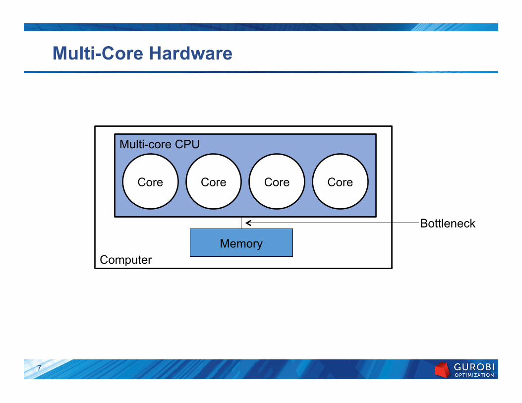
Computer
Multi-core CPU
Multi-Core Hardware
Core Core Core Core
Memory
Bottleneck
7
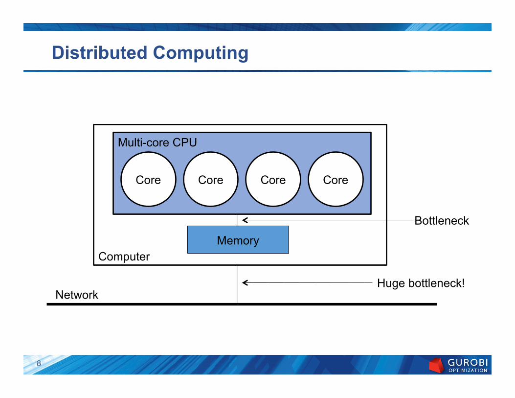
Computer
Multi-core CPU
Distributed Computing
Core Core Core Core
Memory
Network
Bottleneck
Huge bottleneck!
8
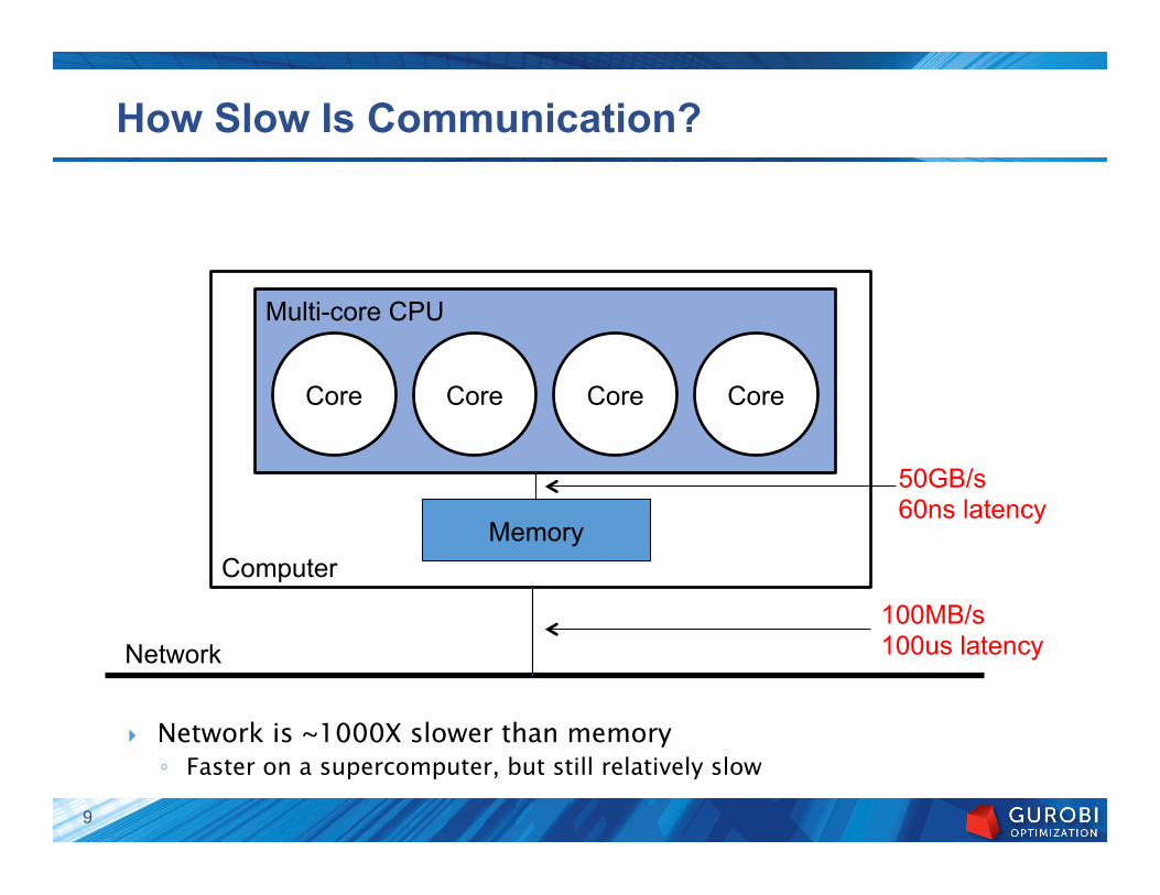
Computer
Multi-core CPU
How Slow Is Communication?
} Network is ~1000X slower than memory ◦ Faster on a supercomputer, but still relatively slow
Core Core Core Core
Memory
Network 100MB/s 100us latency
50GB/s 60ns latency
9

Distributed Algorithms in Gurobi 6.0
} 3 distributed algorithms in version 6.0 ◦ Distributed tuning ◦ Distributed concurrent
� LP (new in 6.0) � MIP ◦ Distributed MIP (new in 6.0)
10
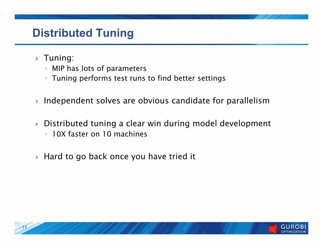
Distributed Tuning
} Tuning: ◦ MIP has lots of parameters ◦ Tuning performs test runs to find better settings
} Independent solves are obvious candidate for parallelism
} Distributed tuning a clear win during model development ◦ 10X faster on 10 machines
} Hard to go back once you have tried it
11

Concurrent Optimization
12

Concurrent Optimization
} Run different algorithms/strategies on different machines/cores ◦ First one that finishes wins
} Nearly ideal for distributed optimization ◦ Communication:
� Send model to each machine � Winner sends solution back
} Concurrent LP: ◦ Different algorithms:
� Primal simplex/dual simplex/barrier } Concurrent MIP: ◦ Different strategies ◦ Default: vary the seed used to break ties
} Easy to customize via concurrent environments
13

MIPLIB 2010 Testset
} MIPLIB 2010 test set… ◦ Set of 361 mixed-integer programming models ◦ Collected by academic/industrial committee
} MIPLIB 2010 benchmark test set… ◦ Subset of the full set - 87 of the 361 models
� Those that were solvable by 2010 codes � (Solvable set now includes 206 of the 361 models)
} Notes: ◦ Definitely not intended as a high-performance computing test set
� More than 2/3 solve in less than 100s � 8 models solve at the root node � ~1/3 solve in fewer than 1000 nodes
14
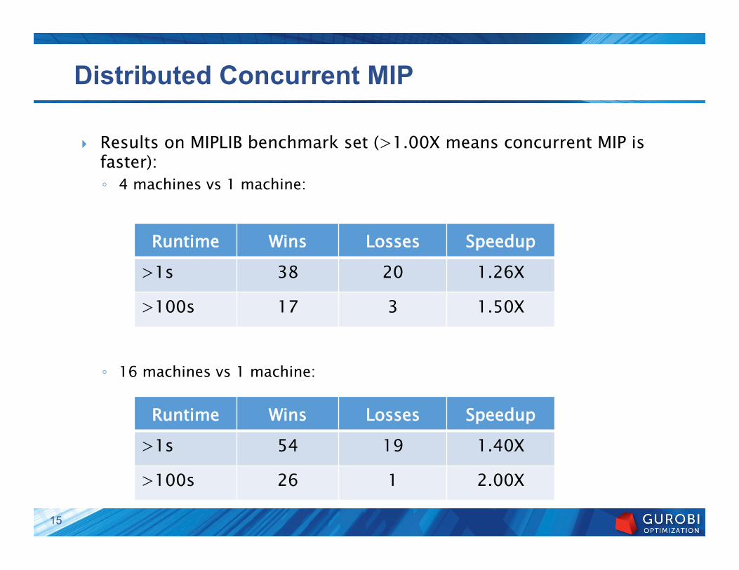
Distributed Concurrent MIP
} Results on MIPLIB benchmark set (>1.00X means concurrent MIP is faster): ◦ 4 machines vs 1 machine:
◦ 16 machines vs 1 machine:
Runtime Wins Losses Speedup >1s 38 20 1.26X
>100s 17 3 1.50X
Runtime Wins Losses Speedup >1s 54 19 1.40X
>100s 26 1 2.00X
15

Customizing Concurrent
} Easy to choose your own settings: ◦ Example – 2 concurrent MIP solves:
� Aggressive cuts on one machine � Aggressive heuristics on second machine
� Java example GRBEnv env0 = model.getConcurrentEnv(0);GRBEnv env1 = model.getConcurrentEnv(1);env0.set(GRB.IntParam.Cuts, 2);env1.set(GRB.DoubleParam.Heuristics, 0.2);model.optimize();model.discardConcurrentEnvs();
� Also supported in C++, .NET, Python and C
16
Distributed MIP
17
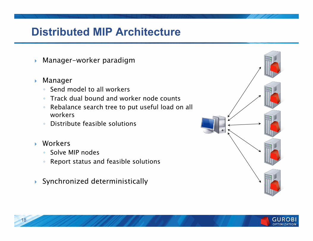
Distributed MIP Architecture
} Manager-worker paradigm
} Manager ◦ Send model to all workers ◦ Track dual bound and worker node counts ◦ Rebalance search tree to put useful load on all
workers ◦ Distribute feasible solutions
} Workers ◦ Solve MIP nodes ◦ Report status and feasible solutions
} Synchronized deterministically
18
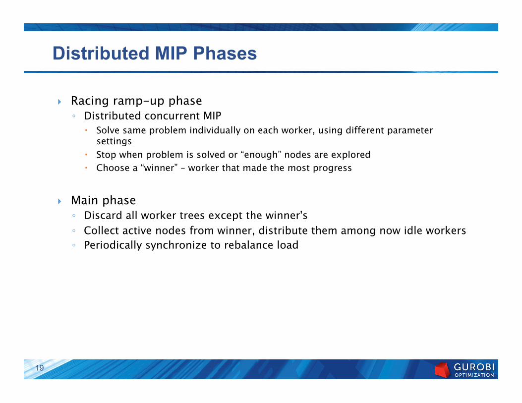
Distributed MIP Phases
} Racing ramp-up phase ◦ Distributed concurrent MIP
� Solve same problem individually on each worker, using different parameter settings
� Stop when problem is solved or “enough” nodes are explored � Choose a “winner” – worker that made the most progress
} Main phase ◦ Discard all worker trees except the winner's ◦ Collect active nodes from winner, distribute them among now idle workers ◦ Periodically synchronize to rebalance load
19

Bad Cases for Distributed MIP
} Easy problems ◦ Why bother with heavy machinery?
} Small search trees ◦ Nothing to gain from parallelism
} Unbalanced search trees ◦ Most nodes sent to workers will be solved immediately
and worker will become idle again
"neos3" solved with SIP (predecessor of SCIP)
Achterberg, Koch, Martin: "Branching Rules Revisited" (2004)
20

Good Cases for Distributed MIP
} Large search trees } Well-balanced search trees ◦ Many nodes in frontier lead to large sub-trees
"vpm2" solved with SIP (predecessor of SCIP)
Achterberg, Koch, Martin: "Branching Rules Revisited" (2004)
21

Performance
22
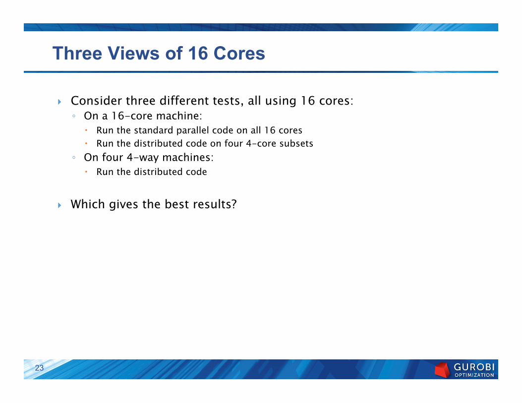
Three Views of 16 Cores
} Consider three different tests, all using 16 cores: ◦ On a 16-core machine:
� Run the standard parallel code on all 16 cores � Run the distributed code on four 4-core subsets
◦ On four 4-way machines: � Run the distributed code
} Which gives the best results?
23

Parallel MIP on 1 Machine
} Use one 16-core machine:
Computer
Multi-core CPU
Memory
Multi-core CPU
Memory
24

Computer
Multi-core CPU Multi-core CPU
Distributed MIP on 1 machine
} Treat one 16-core machine as four 4-core machines:
Memory Memory
25
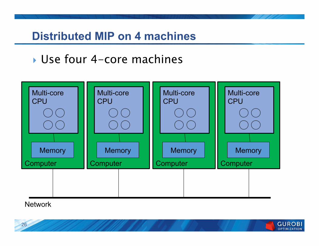
Distributed MIP on 4 machines
} Use four 4-core machines
Computer
Network
Multi-core CPU
Memory
Computer
Multi-core CPU
Memory
Computer
Multi-core CPU
Memory
Computer
Multi-core CPU
Memory
26
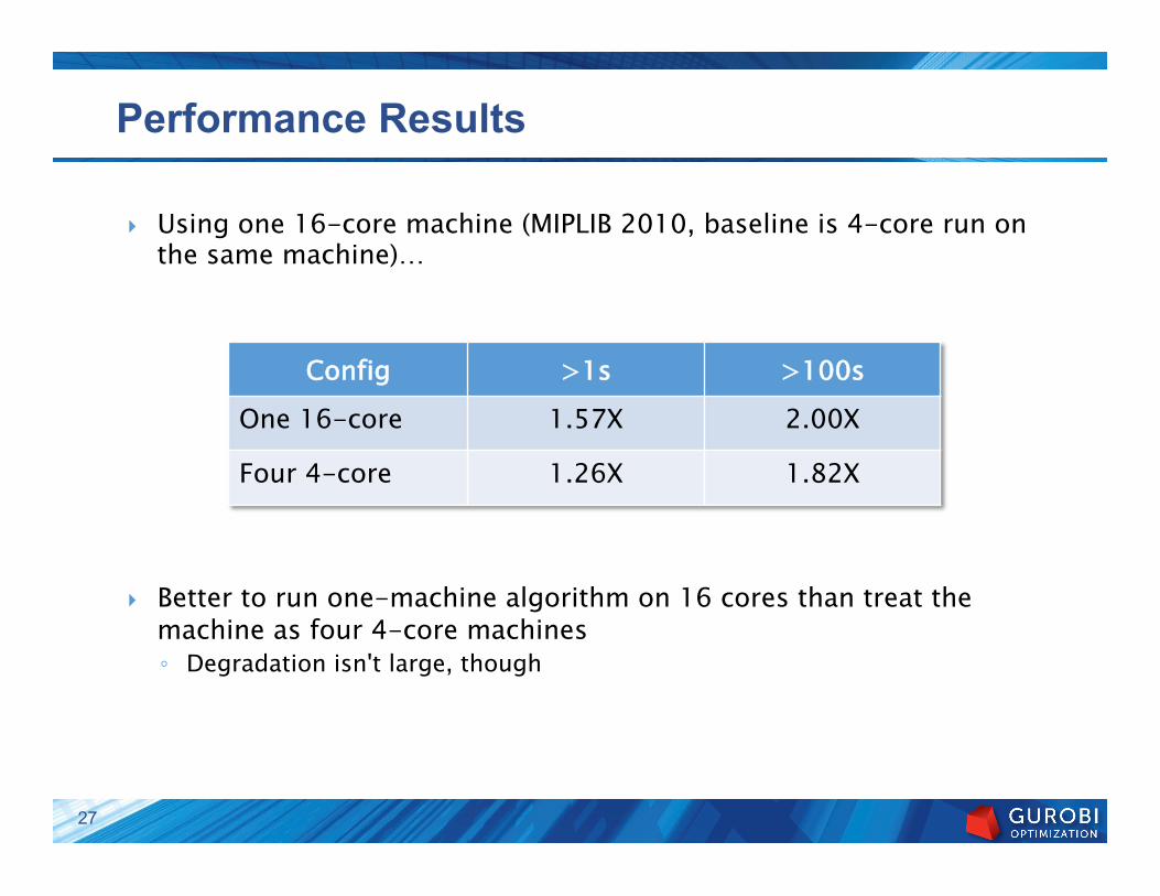
Performance Results
} Using one 16-core machine (MIPLIB 2010, baseline is 4-core run on the same machine)…
} Better to run one-machine algorithm on 16 cores than treat the
machine as four 4-core machines ◦ Degradation isn't large, though
Config >1s >100s One 16-core 1.57X 2.00X
Four 4-core 1.26X 1.82X
27

Performance Results
} Comparing one 16-core machine against four 4-core machines (MIPLIB 2010, baseline is single-machine, 4-core run)…
} Given a choice… ◦ Comparable mean speedups ◦ Other factors…
� Cost: four 4-core machines are much cheaper � Admin: more work to admin 4 machines
Config >1s >100s One 16-core machine 1.57X 2.00X
Four 4-core machines 1.43X 2.09X
28

Distributed Algorithms in 6.0
} MIPLIB 2010 benchmark set ◦ Intel Xeon E3-1240v3 (4-core) CPU ◦ Compare against 'standard' code on 1 machine
Machines >1s >100s
Wins Losses Speedup Wins Losses Speedup
2 40 16 1.14X 20 7 1.27X
4 50 17 1.43X 25 2 2.09X
8 53 19 1.53X 25 2 2.87X
16 52 25 1.58X 25 3 3.15X
29

Some Big Wins
} Model seymour ◦ Hard set covering model from MIPLIB 2010 ◦ 4944 constraints, 1372 (binary) variables, 33K non-zeroes
Machines Nodes Time (s) Speedup 1 476,642 9,267s -
16 1,314,062 1,015s 9.1X
32 1,321,048 633s 14.6X
30
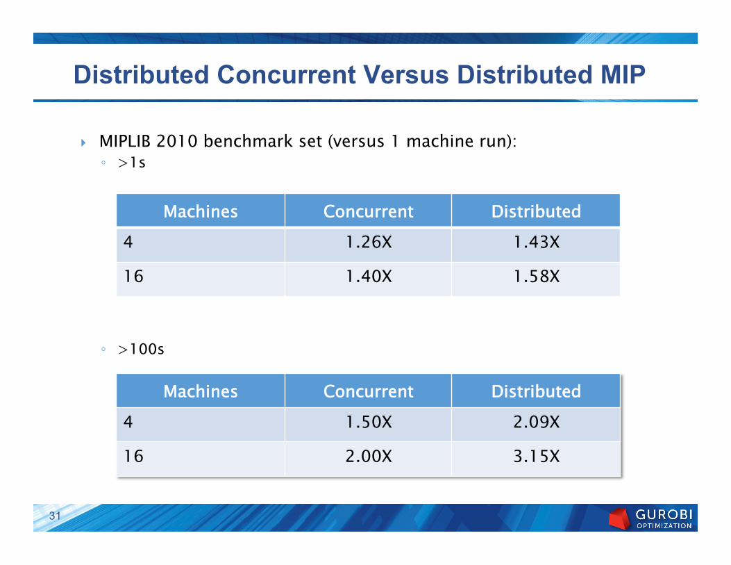
Distributed Concurrent Versus Distributed MIP
} MIPLIB 2010 benchmark set (versus 1 machine run): ◦ >1s
◦ >100s
Machines Concurrent Distributed 4 1.26X 1.43X
16 1.40X 1.58X
Machines Concurrent Distributed 4 1.50X 2.09X
16 2.00X 3.15X
31

} Makes huge improvements in performance possible
} Mean performance improvements are significant but not huge ◦ Some models get big speedups, but many get none ◦ Much better than distributed concurrent ◦ As effective as adding more cores to one box
} Effectively exploiting parallelism remains: ◦ A difficult problem ◦ A focus at Gurobi
Gurobi Distributed MIP
32

Mechanics
33
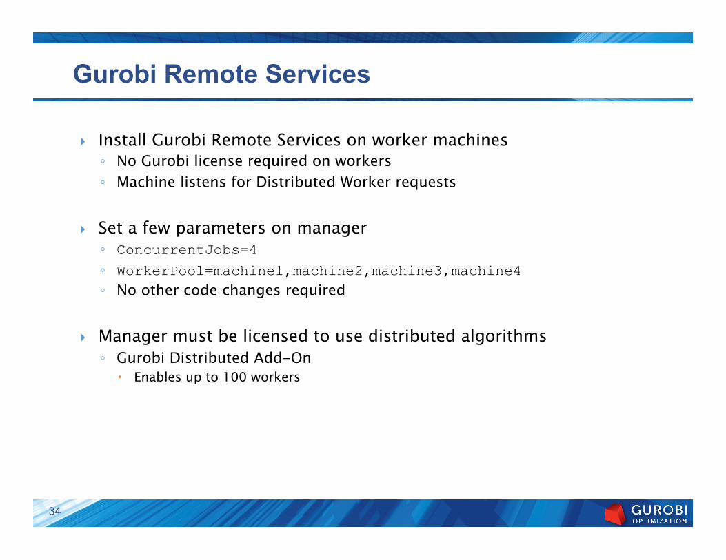
Gurobi Remote Services
} Install Gurobi Remote Services on worker machines ◦ No Gurobi license required on workers ◦ Machine listens for Distributed Worker requests
} Set a few parameters on manager ◦ ConcurrentJobs=4 ◦ WorkerPool=machine1,machine2,machine3,machine4 ◦ No other code changes required
} Manager must be licensed to use distributed algorithms ◦ Gurobi Distributed Add-On
� Enables up to 100 workers
34

Integral Part of Product
} Built on top of Gurobi Compute Server ◦ Only 1500 lines of C code specific to concurrent/distributed MIP
} Built into the product ◦ No special binaries involved
} Bottom line: ◦ Changes to MIP solver automatically apply to distributed code too
� Performance gains in regular MIP also benefit distributed MIP ◦ Distributed MIP will evolve with regular MIP
35
Footnote: GPGPU computing
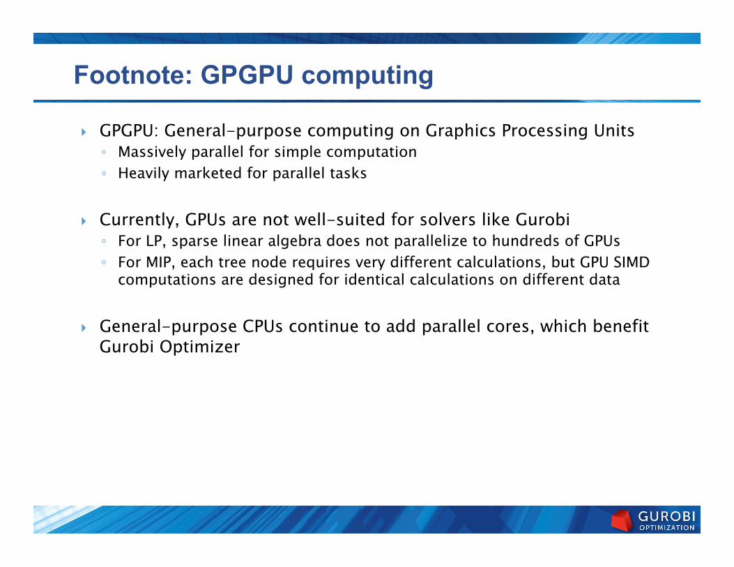
} GPGPU: General-purpose computing on Graphics Processing Units ◦ Massively parallel for simple computation ◦ Heavily marketed for parallel tasks
} Currently, GPUs are not well-suited for solvers like Gurobi ◦ For LP, sparse linear algebra does not parallelize to hundreds of GPUs ◦ For MIP, each tree node requires very different calculations, but GPU SIMD
computations are designed for identical calculations on different data
} General-purpose CPUs continue to add parallel cores, which benefit Gurobi Optimizer
Distributed Optimization Licensing
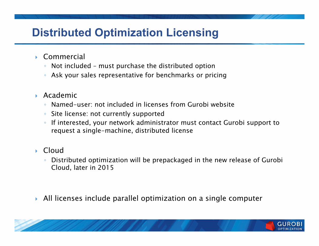
} Commercial ◦ Not included – must purchase the distributed option ◦ Ask your sales representative for benchmarks or pricing
} Academic ◦ Named-user: not included in licenses from Gurobi website ◦ Site license: not currently supported ◦ If interested, your network administrator must contact Gurobi support to
request a single-machine, distributed license
} Cloud ◦ Distributed optimization will be prepackaged in the new release of Gurobi
Cloud, later in 2015
} All licenses include parallel optimization on a single computer

Thank YouSend us an email at [email protected] if you have questions or would like additional information.


![The Gurobi Optimizer - NUOR · E.g., at the root node Initialize pseudo-costs [Linderoth & Savelsbergh, 1999] Always compute up/down cost (using strong branching) for new fractional](https://static.fdocuments.us/doc/165x107/602a28037e906a39a9689cc0/the-gurobi-optimizer-nuor-eg-at-the-root-node-initialize-pseudo-costs-linderoth.jpg)