What's New in Gurobi 9
41
What's New in Gurobi 9.0 Webinar Tobias Achterberg 17/18 December 2019
Transcript of What's New in Gurobi 9

What's New in Gurobi 9.0Webinar
Tobias Achterberg
17/18 December 2019

Highlights
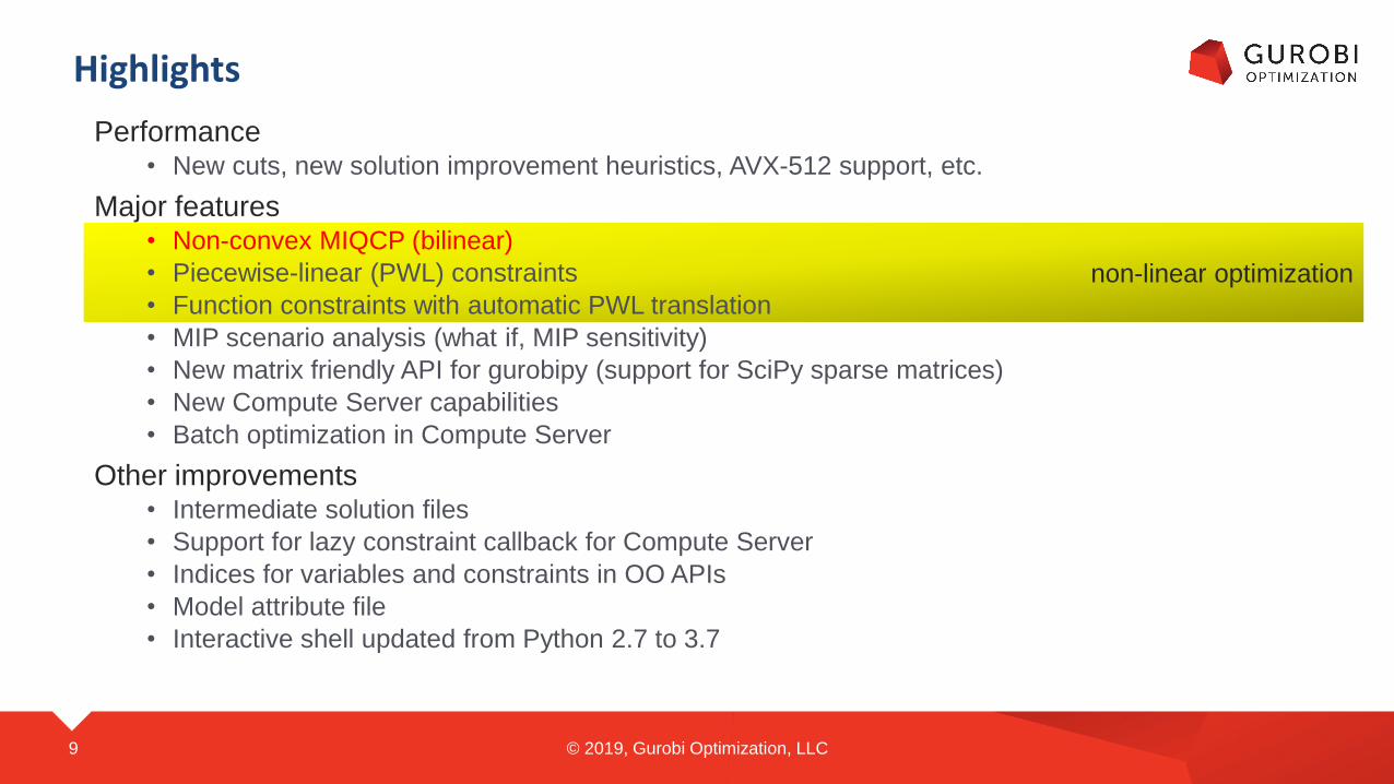
Performance• New cuts, new solution improvement heuristics, AVX-512 support, etc.
Major features• Non-convex MIQCP (bilinear)
• Piecewise-linear (PWL) constraints
• Function constraints with automatic PWL translation
• MIP scenario analysis (what if, MIP sensitivity)
• New matrix friendly API for gurobipy (support for SciPy sparse matrices)
• New Compute Server capabilities
• Batch optimization in Compute Server
Other improvements• Intermediate solution files
• Support for lazy constraint callback for Compute Server
• Indices for variables and constraints in OO APIs
• Model attribute file
• Interactive shell updated from Python 2.7 to 3.7
2 © 2019, Gurobi Optimization, LLC

Highlights
Performance• New cuts, new solution improvement heuristics, AVX-512 support, etc.
Major features• Non-convex MIQCP (bilinear)
• Piecewise-linear (PWL) constraints
• Function constraints with automatic PWL translation
• MIP scenario analysis (what if, MIP sensitivity)
• New matrix friendly API for gurobipy (support for SciPy sparse matrices)
• New Compute Server capabilities
• Batch optimization in Compute Server
Other improvements• Intermediate solution files
• Support for lazy constraint callback for Compute Server
• Indices for variables and constraints in OO APIs
• Model attribute file
• Interactive shell updated from Python 2.7 to 3.7
3 © 2019, Gurobi Optimization, LLC
LP Performance
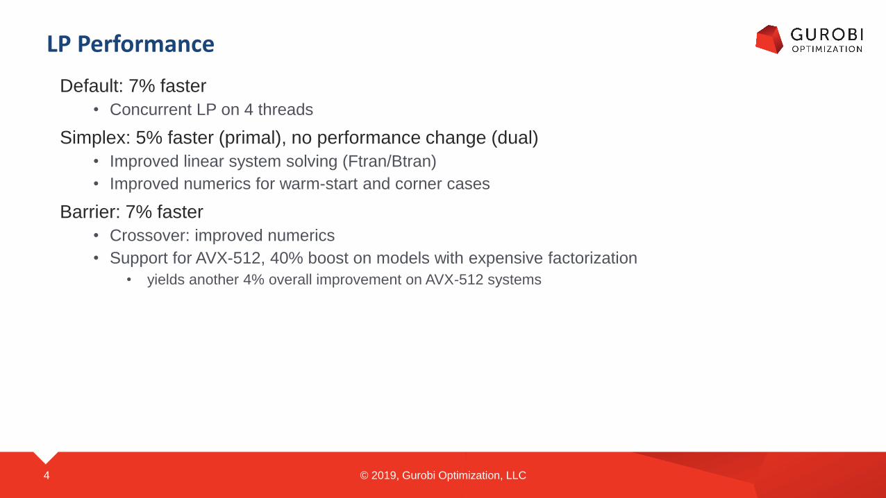
Default: 7% faster
• Concurrent LP on 4 threads
Simplex: 5% faster (primal), no performance change (dual)
• Improved linear system solving (Ftran/Btran)
• Improved numerics for warm-start and corner cases
Barrier: 7% faster
• Crossover: improved numerics
• Support for AVX-512, 40% boost on models with expensive factorization
• yields another 4% overall improvement on AVX-512 systems
© 2019, Gurobi Optimization, LLC4

MIP Performance
MILP: 18% faster (26% faster on models that take >100 seconds)
• Heuristics:• new solution improvement heuristic
• new "lurking bounds" heuristic
• extended some heuristics to work for models with SOS constraints
• Presolve:• implied product detection
• detect implicit piece-wise linear functions
• sparsify objective function
• substitute sub-expressions in presolve to sparsify constraints
• better work limits in constraint sparsification
• improved parallel column/row presolve reduction
• activate SOS2 to big-M translation in some cases
• Additional improvements:• improved disconnected components
• extended disconnected components detection to work for models with SOS constraints
• reduced wait time in parallel synchronization by more flexible work load distribution
• propagate objective function in node probing
© 2019, Gurobi Optimization, LLC5
• Cuts:
• new RLT cuts
• new BQP cuts
• new RelaxLift cuts
• second type of "SubMIP" cuts
• use LP to find another aggregation for MIR cut separator
• randomize aggregation order in MIR cut separator
• try more scaling factors in MIR cut separator
• more aggressive cover cut separation
• occasionally separate "close cuts"
• tuned cut loop abort criteria for main and parallel cut loops
• improved dual bound updates from parallel root cut loops
• improved cut selection
• improved performance of zero-half and mod-k cut separators
• limit effort in GUB cover and network cut separation procedures
• limit effort in some very expensive cut separation procedure
• fixed a performance issue in symmetry cuts

New Solution Improvement Heuristics
Heuristics have improved significantly
Still opportunities to do better
• Particularly when the relaxation isn’t a good guide
Better improvement heuristics
• ImproveStartGap, ImproveStartNodes, ImproveStartTime
• Comparison against old version on a set of difficult models
• New scheme finds better solution on 83% of models
© 2019, Gurobi Optimization, LLC6
Convex MIQP and MIQCP Performance
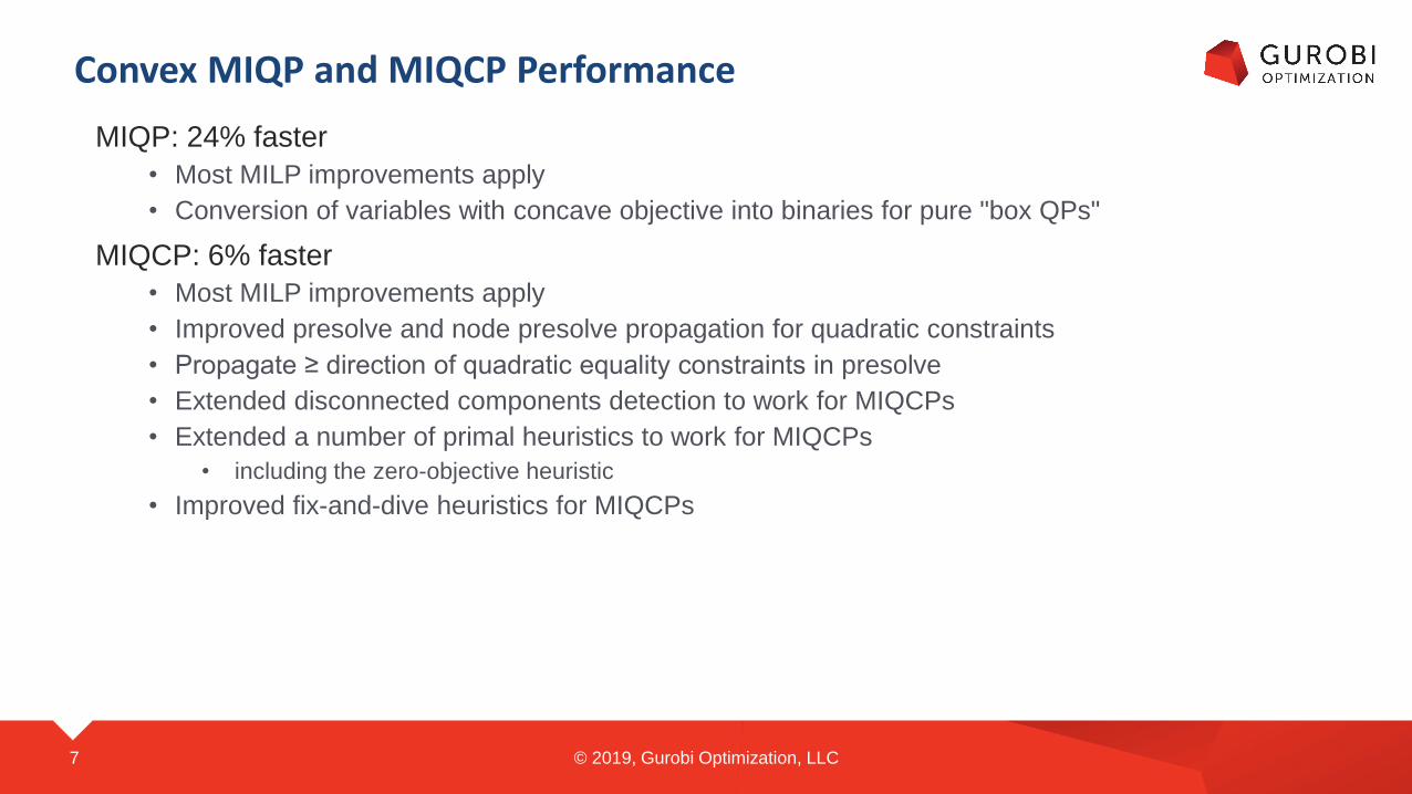
MIQP: 24% faster
• Most MILP improvements apply
• Conversion of variables with concave objective into binaries for pure "box QPs"
MIQCP: 6% faster
• Most MILP improvements apply
• Improved presolve and node presolve propagation for quadratic constraints
• Propagate ≥ direction of quadratic equality constraints in presolve
• Extended disconnected components detection to work for MIQCPs
• Extended a number of primal heuristics to work for MIQCPs
• including the zero-objective heuristic
• Improved fix-and-dive heuristics for MIQCPs
© 2019, Gurobi Optimization, LLC7

© 2019, Gurobi Optimization, LLC8
Major Features
non-linear optimization
Highlights
Performance• New cuts, new solution improvement heuristics, AVX-512 support, etc.
Major features• Non-convex MIQCP (bilinear)
• Piecewise-linear (PWL) constraints
• Function constraints with automatic PWL translation
• MIP scenario analysis (what if, MIP sensitivity)
• New matrix friendly API for gurobipy (support for SciPy sparse matrices)
• New Compute Server capabilities
• Batch optimization in Compute Server
Other improvements• Intermediate solution files
• Support for lazy constraint callback for Compute Server
• Indices for variables and constraints in OO APIs
• Model attribute file
• Interactive shell updated from Python 2.7 to 3.7
9 © 2019, Gurobi Optimization, LLC

Non-Convex QP, QCP, MIQP, and MIQCP
A lot of applications
• Pooling problem (blending problem is LP, pooling introduces intermediate pools → bilinear)
• Petrochemical industry (oil refinery: constraints on ratio of components in tanks)
• Wastewater treatment
• Emissions regulation
• Agricultural / food industry (blending based on pre-mix products)
• Etc.
10 © 2019, Gurobi Optimization, LLC

Non-Convex QP, QCP, MIQP, and MIQCP
Prior Gurobi versions: remaining Q constraints and objective after presolve needed to be convex
If 𝑄 is positive semi-definite (PSD) then 𝑥𝑇𝑄𝑥 ≤ 𝑏 is convex
• 𝑄 is PSD if and only if 𝑥𝑇𝑄𝑥 ≥ 0 for all 𝑥
But 𝑥𝑇𝑄𝑥 ≤ 𝑏 can also be convex in certain other cases, e.g., second order cones (SOCs)
Copyright © 2019, Gurobi Optimization, LLC11
convex
−𝑦 + 𝑥2 ≤ 0
𝑥𝑇𝑄𝑥 ≤ 𝑏
non-convex
−𝑦 − 𝑥2 ≤ 0
𝑥2 + 𝑦2 − 𝑧2 ≤ 0, 𝑧 ≥ 0: at level 𝑧, 𝑥, 𝑦 is a disc with radius 𝑧
SOC: 𝑥12 +⋯+ 𝑥𝑛
2 − 𝑧2 ≤ 0
Non-Convex QP, QCP, MIQP, and MIQCP
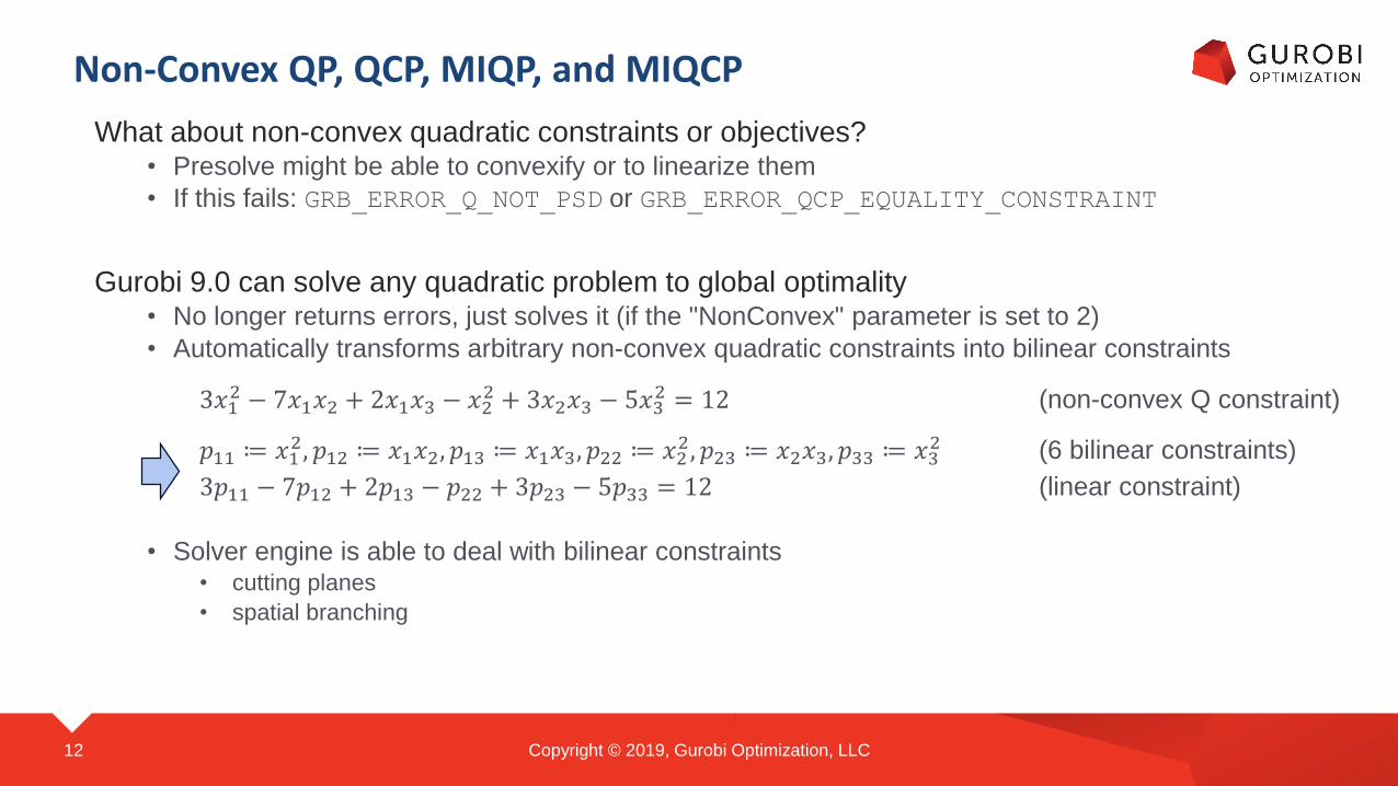
What about non-convex quadratic constraints or objectives?• Presolve might be able to convexify or to linearize them
• If this fails: GRB_ERROR_Q_NOT_PSD or GRB_ERROR_QCP_EQUALITY_CONSTRAINT
Gurobi 9.0 can solve any quadratic problem to global optimality• No longer returns errors, just solves it (if the "NonConvex" parameter is set to 2)
• Automatically transforms arbitrary non-convex quadratic constraints into bilinear constraints
3𝑥12 − 7𝑥1𝑥2 + 2𝑥1𝑥3 − 𝑥2
2 + 3𝑥2𝑥3 − 5𝑥32 = 12 (non-convex Q constraint)
𝑝11 ≔ 𝑥12, 𝑝12 ≔ 𝑥1𝑥2, 𝑝13 ≔ 𝑥1𝑥3, 𝑝22 ≔ 𝑥2
2, 𝑝23 ≔ 𝑥2𝑥3, 𝑝33 ≔ 𝑥32 (6 bilinear constraints)
3𝑝11 − 7𝑝12 + 2𝑝13 − 𝑝22 + 3𝑝23 − 5𝑝33 = 12 (linear constraint)
• Solver engine is able to deal with bilinear constraints• cutting planes
• spatial branching
Copyright © 2019, Gurobi Optimization, LLC12

Non-Convex QP, QCP, MIQP, and MIQCP
Algorithmic treatment of bilinear constraints
• General form: 𝑎𝑇𝑧 + 𝑑𝑥𝑦 ≦ 𝑏 (linear sum plus single product term, inequality or equation)
Consider square case (𝑥 = 𝑦):
convex
−𝑧 + 𝑥2 ≤ 0non-convex
−𝑧 − 𝑥2 ≤ 0
Copyright © 2019, Gurobi Optimization, LLC13

Non-Convex QP, QCP, MIQP, and MIQCP
Algorithmic treatment of bilinear constraints
• General form: 𝑎𝑇𝑧 + 𝑑𝑥𝑦 ≦ 𝑏 (linear sum plus single product term, inequality or equation)
Consider square case (𝑥 = 𝑦):
convex
−𝑧 + 𝑥2 ≤ 0non-convex
−𝑧 − 𝑥2 ≤ 0
easy: add tangent cuts
Copyright © 2019, Gurobi Optimization, LLC14

Non-Convex QP, QCP, MIQP, and MIQCP
Algorithmic treatment of bilinear constraints
• General form: 𝑎𝑇𝑧 + 𝑑𝑥𝑦 ≦ 𝑏 (linear sum plus single product term, inequality or equation)
Consider square case (𝑥 = 𝑦):
non-convex
−𝑧 − 𝑥2 ≤ 0
Copyright © 2019, Gurobi Optimization, LLC15

Non-Convex QP, QCP, MIQP, and MIQCP
Algorithmic treatment of bilinear constraints
• General form: 𝑎𝑇𝑧 + 𝑑𝑥𝑦 ≦ 𝑏 (linear sum plus single product term, inequality or equation)
Consider square case (𝑥 = 𝑦):
non-convex
−𝑧 − 𝑥2 ≤ 0
Copyright © 2019, Gurobi Optimization, LLC16

Non-Convex QP, QCP, MIQP, and MIQCP
Algorithmic treatment of bilinear constraints
• General form: 𝑎𝑇𝑧 + 𝑑𝑥𝑦 ≦ 𝑏 (linear sum plus single product term, inequality or equation)
Consider square case (𝑥 = 𝑦):
non-convex
−𝑧 − 𝑥2 ≤ 0
branching
𝑥 ≤ 0 or 𝑥 ≥ 0
update relaxation locally
Copyright © 2019, Gurobi Optimization, LLC17
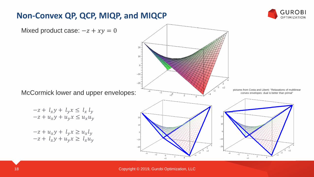
Non-Convex QP, QCP, MIQP, and MIQCP
Mixed product case: −𝑧 + 𝑥𝑦 = 0
McCormick lower and upper envelopes:
−𝑧 + 𝑙𝑥𝑦 + 𝑙𝑦𝑥 ≤ 𝑙𝑥 𝑙𝑦−𝑧 + 𝑢𝑥𝑦 + 𝑢𝑦𝑥 ≤ 𝑢𝑥𝑢𝑦
−𝑧 + 𝑢𝑥𝑦 + 𝑙𝑦𝑥 ≥ 𝑢𝑥𝑙𝑦−𝑧 + 𝑙𝑥𝑦 + 𝑢𝑦𝑥 ≥ 𝑙𝑥𝑢𝑦
pictures from Costa and Liberti: "Relaxations of multilinear
convex envelopes: dual is better than primal"
Copyright © 2019, Gurobi Optimization, LLC18

Non-Convex QP, QCP, MIQP, and MIQCP
Mixed product case: −𝑧 + 𝑥𝑦 = 0
McCormick lower and upper envelopes:
−𝑧 + 𝑙𝑥𝑦 + 𝑙𝑦𝑥 ≤ 𝑙𝑥 𝑙𝑦−𝑧 + 𝑢𝑥𝑦 + 𝑢𝑦𝑥 ≤ 𝑢𝑥𝑢𝑦
−𝑧 + 𝑢𝑥𝑦 + 𝑙𝑦𝑥 ≥ 𝑢𝑥𝑙𝑦−𝑧 + 𝑙𝑥𝑦 + 𝑢𝑦𝑥 ≥ 𝑙𝑥𝑢𝑦
coefficients depend
on local bounds
pictures from Costa and Liberti: "Relaxations of multilinear
convex envelopes: dual is better than primal"
Copyright © 2019, Gurobi Optimization, LLC19

Non-Convex QP, QCP, MIQP, and MIQCP
Algorithmic ingredients
• Presolve translation of general non-convex Q constraints into bilinear constraints
• McCormick relaxation
• Spatial branching (branching on continuous variables)
• "Adaptive constraints"
• automatically modify coefficients in McCormick relaxation after local bound change
• alternative to adding more and more locally valid cuts
• Cutting planes
• RLT cuts (RLT = Reformulation Linearization Technique)
• BQP cuts (BQP = Boolean Quadric Polytope)
• not yet in Gurobi: SDP cuts (SDP = Semi-Definite Program)
• ...
Can also use techniques for MILP
• Detection of linearization of products with a binary variable
• Results in performance improvement on MILP: RLT cuts and BQP cuts
Copyright © 2019, Gurobi Optimization, LLC20
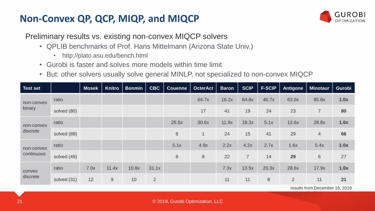
Non-Convex QP, QCP, MIQP, and MIQCP
Preliminary results vs. existing non-convex MIQCP solvers
• QPLIB benchmarks of Prof. Hans Mittelmann (Arizona State Univ.)
• http://plato.asu.edu/bench.html
• Gurobi is faster and solves more models within time limit
• But: other solvers usually solve general MINLP, not specialized to non-convex MIQCP
21 © 2019, Gurobi Optimization, LLC
Test set Mosek Knitro Bonmin CBC Couenne OcterAct Baron SCIP F-SCIP Antigone Minotaur Gurobi
non-convex
binary
ratio 64.7x 16.2x 64.8x 46.7x 63.0x 85.8x 1.0x
solved (80) 17 41 19 24 23 7 80
non-convex
discrete
ratio 25.5x 30.6x 11.9x 18.3x 5.1x 12.6x 28.8x 1.0x
solved (88) 8 1 24 15 41 29 4 66
non-convex
continuous
ratio 5.1x 4.9x 2.2x 4.2x 2.7x 1.6x 5.4x 1.0x
solved (49) 8 8 22 7 14 29 6 27
convex
discrete
ratio 7.0x 11.4x 10.8x 31.1x 7.3x 13.5x 20.3x 28.6x 17.9x 1.0x
solved (31) 12 9 10 2 11 11 8 2 11 21
results from December 16, 2019

non-linear optimization
Highlights
Performance• New cuts, new solution improvement heuristics, AVX-512 support, etc.
Major features• Non-convex MIQCP (bilinear)
• Piecewise-linear (PWL) constraints
• Function constraints with automatic PWL translation
• MIP scenario analysis (what if, MIP sensitivity)
• New matrix friendly API for gurobipy (support for SciPy sparse matrices)
• New Compute Server capabilities
• Batch optimization in Compute Server
Other improvements• Intermediate solution files
• Support for lazy constraint callback for Compute Server
• Indices for variables and constraints in OO APIs
• Model attribute file
• Interactive shell updated from Python 2.7 to 3.7
22 © 2019, Gurobi Optimization, LLC

Piecewise-Linear (PWL) Constraints
A new type of general constraint
Users specify the supporting points as a list of (x,y) tuples
23 © 2019, Gurobi Optimization, LLC
supporting
points
may have jump
extended towards
infinity with same slope
𝑦 = 𝑃𝑊𝐿 𝑥; 𝑥1, 𝑦1 , … , 𝑥𝑛, 𝑦𝑛

Piecewise-Linear (PWL) Constraints
A new type of general constraint
Users specify the supporting points as a list of (x,y) tuples
Example
• 𝑦 = 𝑒𝑥, 0 ≤ 𝑥 ≤ 1• To approximate this as PWL constraint with 100 pieces, generate 101 points (xpts, ypts):
0, 𝑒0 , 0.01, 𝑒0.01 , … , 1, 𝑒1
• Python code:n = 100xpts = [1.0*k/n for k in range(n+1)]ypts = [math.exp(xpts[k]) for k in range(n+1)]
model = Model("pwltest")x = model.addVar(lb=0, ub=1, name="x")y = model.addVar(name="y")gc = model.addGenConstrPWL(x, y, xpts, ypts, "gc")model.setObjective(-2*x + y)model.optimize()
24 © 2019, Gurobi Optimization, LLC

y exp x
x y
Piecewise-Linear (PWL) Constraints
© 2019, Gurobi Optimization, LLC25
Optimize a model with 0 rows, 2 columns and 0 nonzeros
Model fingerprint: 0xe289cdc2
Model has 1 general constraint
Variable types: 2 continuous, 0 integer (0 binary)
...
Nodes | Current Node | Objective Bounds | Work
Expl Unexpl | Obj Depth IntInf | Incumbent BestBd Gap | It/Node Time
0 0 cutoff 0 0.61372 0.61372 0.00% - 0s
...
Optimal solution found (tolerance 1.00e-04)
Violations: const 0.0000e+00, bound 0.0000e+00, int 0.0000e+00, genconstr 0.0000e+00
Best objective 6.137155332431e-01, best bound 6.137155332431e-01, gap 0.0000%
gurobi> print x.X
0.69
gurobi> print y.X
1.99371553324
(0.69, 1.9937)
min -2x+y
Function Constraints with Automatic PWL Translation
𝑦 = 𝑓(𝑥)
Support: polynomial, log 𝑥 , log𝑎(𝑥), 𝑒𝑥, 𝑎𝑥, 𝑥𝑎, sin(𝑥), cos 𝑥 , tan(𝑥)
Another new type of general constraint
Example
• 𝑦 = 𝑒𝑥, 0 ≤ 𝑥 ≤ 1
• Python code: gc = model.addGenConstrExp(x, y, name=“gc”)
Gurobi will automatically compute breakpoints and perform PWL translation
• Smart translation for periodic functions sin(), cos(), and tan()
• Use actual functions during presolve
• Bound strengthening in presolve may lead to more efficient PWL translation
26 © 2019, Gurobi Optimization, LLC
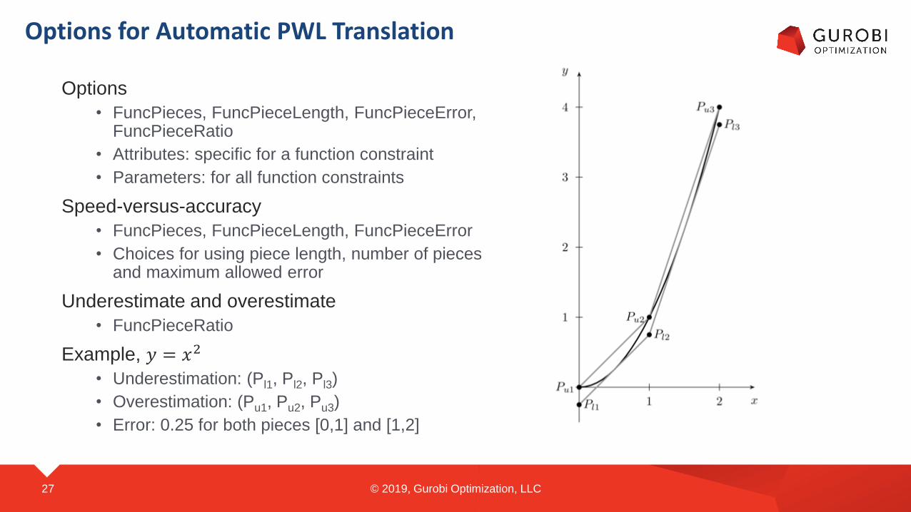
Options for Automatic PWL Translation
Options
• FuncPieces, FuncPieceLength, FuncPieceError, FuncPieceRatio
• Attributes: specific for a function constraint
• Parameters: for all function constraints
Speed-versus-accuracy
• FuncPieces, FuncPieceLength, FuncPieceError
• Choices for using piece length, number of pieces and maximum allowed error
Underestimate and overestimate
• FuncPieceRatio
Example, 𝑦 = 𝑥2
• Underestimation: (Pl1, Pl2, Pl3)
• Overestimation: (Pu1, Pu2, Pu3)
• Error: 0.25 for both pieces [0,1] and [1,2]
27 © 2019, Gurobi Optimization, LLC

Non-linear Capability
Theory• Multivariate polynomials can be decomposed into bilinear functions
• 𝑧 = 𝑥4𝑦2
• Let 𝑢 = 𝑥2, 𝑣 = 𝑢2, 𝑤 = 𝑦2 (bilinear)
• Then 𝑧 = 𝑣𝑤 (bilinear)
• PWL constraints allow to approximate single-variable non-linear functions
• Solve wide range of non-linear programming problems to global optimality
• e.g., z = 𝑠𝑖𝑛 𝑥2𝑦 ∙ 𝑒𝑥+𝑦2
Reality• Errors will amplify for decomposing/combining
• Errors for PWL approximation can be big
• Example:
• 𝑦 = 𝑥 − 0.25, 𝑦 = 𝑥2
• 𝑦 = 𝑥 − 0.25 is for line (Pl1, P, Pl2)
• 𝑃 = (𝑥, 𝑦) = (0.5, 0.25) is feasible
• PWL approximation of 𝑦 = 𝑥2 with line segments (Pu1, Pu2, Pu3)
• 𝑦 = 0.5 at 𝑥 = 0.5, Q(0.5, 0.5) is quite far from P(0.5, 0.25)
• Infeasible
• FuncPieceLength=1 is too big: largest error = 0.25 is too big to be feasible
28 © 2019, Gurobi Optimization, LLC
dealing with uncertainty
Highlights
Performance• New cuts, new solution improvement heuristics, AVX-512 support, etc.
Major features• Non-convex MIQCP (bilinear)
• Piecewise-linear (PWL) constraints
• Function constraints with automatic PWL translation
• MIP scenario analysis (what if, MIP sensitivity)
• New matrix friendly API for gurobipy (support for SciPy sparse matrices)
• New Compute Server capabilities
• Batch optimization in Compute Server
Other improvements• Intermediate solution files
• Support for lazy constraint callback for Compute Server
• Indices for variables and constraints in OO APIs
• Model attribute file
• Interactive shell updated from Python 2.7 to 3.7
29 © 2019, Gurobi Optimization, LLC

MIP Scenario Analysis
Motivation• Math model is usually an approximation for the real-world application
• Inputs are often approximations e.g. forecasted demands
• Business condition or environment may change
• Important to know the sensitivity of the computed solution to the changes, e.g.• What if the demand for this item increases from 10 to 12?
Wrong approach• Fix all integer variables, solve fixed model as LP, look at reduced costs and duals of fixed LP
• Gives bogus results! Does not make sense from mathematical point of view!
Our approach• Have a base model
• Use attributes to specify a set of scenarios• each scenario is described by changes to the base model
• currently supported changes: objective coefficients, variable bounds, linear constraint right hand sides
• Compute optimal solutions for all scenarios
• Solutions provide the insight into how the solution would change for different scenarios
30 © 2019, Gurobi Optimization, LLC

MIP Scenario Analysis
Simple approach
• Solve each scenario as an independent MIP
• Old example: sensitivity.py
New approach in Gurobi 9.0
• Convenient to define scenarios
• use attributes
• example sensitivity.py is rewritten by using the new feature
• Performance
• faster
• may add distributed version with Compute Server in a future version
• information, such as objective bounds, feasible solutions for each scenario, still available even if you stop early (e.g., due to time limit)
31 © 2019, Gurobi Optimization, LLC

Dealing With Uncertainty
MIP Scenario Analysis• Find optimal solution for each individual scenario
• Each solution may be infeasible for other scenarios
• Analyze business model: how sensitive are best decisions w.r.t. input data?
• MIP-version of LP sensitivity analysis
Stochastic Optimization• Find one solution that is optimal w.r.t. expected value over all scenarios
• User needs to specify probabilities for each scenario• or: provide probability density functions for random variables
Robust Optimization• Find one solution that is optimal in worst case scenario
• Model coefficients are not fixed but user specifies ranges• more generally: coefficients should be in a specified convex set
32 © 2019, Gurobi Optimization, LLC
data scientists, engineers
Highlights
Performance• New cuts, new solution improvement heuristics, AVX-512 support, etc.
Major features• Non-convex MIQCP (bilinear)
• Piecewise-linear (PWL) constraints
• Function constraints with automatic PWL translation
• MIP scenario analysis (what if, MIP sensitivity)
• New matrix friendly API for gurobipy (support for SciPy sparse matrices)
• New Compute Server capabilities
• Batch optimization in Compute Server
Other improvements• Intermediate solution files
• Support for lazy constraint callback for Compute Server
• Indices for variables and constraints in OO APIs
• Model attribute file
• Interactive shell updated from Python 2.7 to 3.7
33 © 2019, Gurobi Optimization, LLC

New Matrix Friendly API for gurobipy
About Python
• A very popular programming language
• Huge library
• Standard library
• 3rd party packages with simple package manager
• A top language for data science
Data scientists and engineers are used to work with matrices
• Large fraction of them use Python with NumPy and SciPy
gurobipy accepts NumPy’s ndarrays and scipy.sparse matrices as input
• More convenient if the underlying model is naturally expressed with matrices
• Faster because no modeling objects for individual linear expressions are created
• API offers two layers (only linear constraints shown here):
• Add matrix constraints directly from the data through Model.addMConstrs(A, x, sense, b)
• Use matrix variable modeling objects x = Model.addMVar(shape), add constraints through Model.addConstr(A @ x <= b)
34 © 2019, Gurobi Optimization, LLC

Python Matrix API – A Tiny Example
mip1.py: algebraic syntax
import gurobipy as gp
from gurobipy import GRB
m = gp.Model("mip1")
x = m.addVar(vtype=GRB.BINARY, name="x")
y = m.addVar(vtype=GRB.BINARY, name="y")
z = m.addVar(vtype=GRB.BINARY, name="z")
m.setObjective(x + y + 2 * z, GRB.MAXIMIZE)
m.addConstr(x + 2 * y + 3 * z <= 4, "c0")
m.addConstr(x + y >= 1, "c1")
m.optimize()
matrix1.py: matrix expressions
import numpy as npimport scipy.sparse as spimport gurobipy as gpfrom gurobipy import GRB
m = gp.Model("matrix1")
x = m.addMVar(shape=3, vtype=GRB.BINARY, name="x")
obj = np.array([1.0, 1.0, 2.0])m.setObjective(obj @ x, GRB.MAXIMIZE)
data = np.array([1.0, 2.0, 3.0, -1.0, -1.0])row = np.array([0, 0, 0, 1, 1])col = np.array([0, 1, 2, 0, 1])A = sp.csr_matrix((data, (row, col)), shape=(2, 3))
rhs = np.array([4.0, -1.0])
m.addConstr(A @ x <= rhs, name="c")
m.optimize()
© 2019 Gurobi Optimization, LLC35

corporate IT, private cloud, offline solves
Highlights
Performance• New cuts, new solution improvement heuristics, AVX-512 support, etc.
Major features• Non-convex MIQCP (bilinear)
• Piecewise-linear (PWL) constraints
• Function constraints with automatic PWL translation
• MIP scenario analysis (what if, MIP sensitivity)
• New matrix friendly API for gurobipy (support for SciPy sparse matrices)
• Cluster Manager
• Batch optimization in Compute Server
Other improvements• Intermediate solution files
• Support for lazy constraint callback for Compute Server
• Indices for variables and constraints in OO APIs
• Model attribute file
• Interactive shell updated from Python 2.7 to 3.7
36 © 2019, Gurobi Optimization, LLC

Cluster Manager
Administer cluster of Gurobi Compute Servers
• IT department can control and track cluster size and work-load
• Users can monitor and manage their jobs
User management
• Allows to assign users to different roles (user, admin, cluster admin)
• Improved security and API keys
Web UI for on-premise
• User-friendly graphical interface for administrators and users
Job history
• Statistics and logs for individual jobs
Batch mode support
• Offline optimization for long running jobs
• Client application may disconnect and retrieve results later
37 © 2019, Gurobi Optimization, LLC
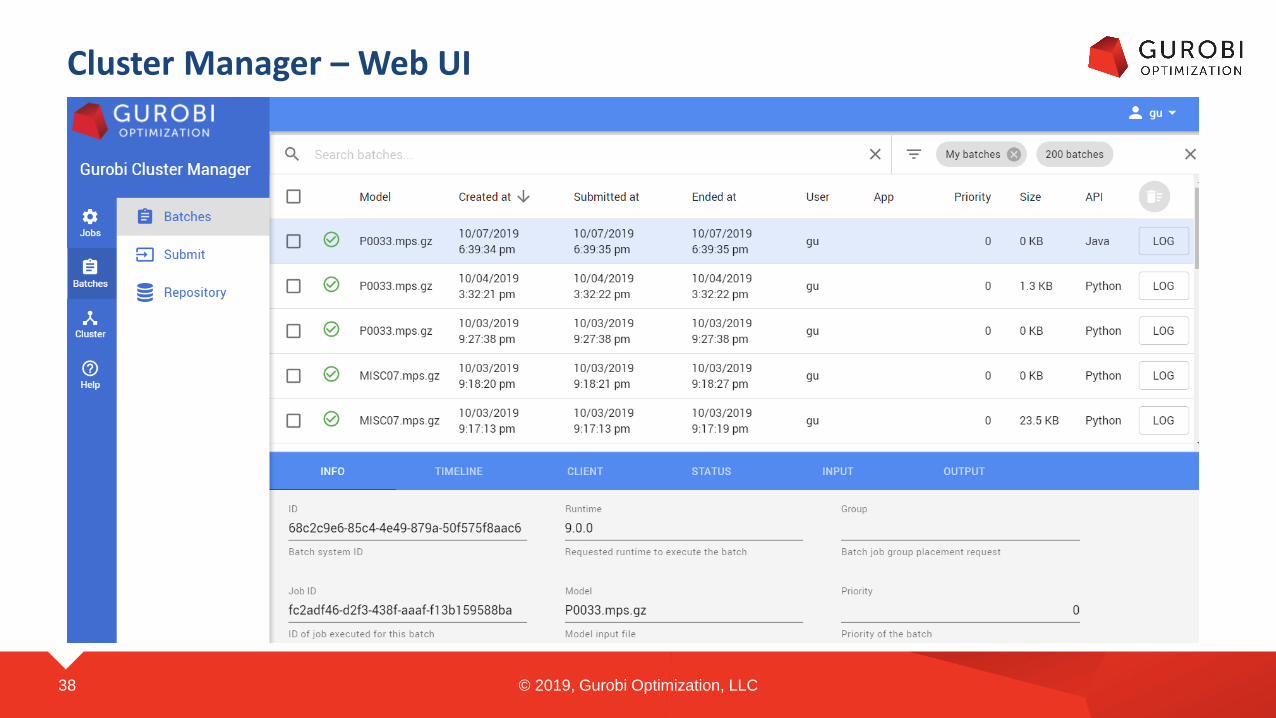
Cluster Manager – Web UI
38 © 2019, Gurobi Optimization, LLC

Batch Optimization in Cluster Manager
Motivation
• Compute Server allows the client code to off-load computing work to a server
• A MIP often takes very long to solve
• requiring the client code to wait may not be convenient
• Feature request
• allow client code to disconnect from the Compute Server and to shut down
• later, client code should be able to reconnect and retrieve results
Technical Problem
• Reconnecting to the server creates a mapping problem
• variable and constraint objects at client side are gone
Our solution
• Create models locally at client site
• Tag a set of relevant variables and constraints
• Submit the model to Compute Server, get batch ID and disconnect
• Use job ID to query status and solution in JSON format
39 © 2019, Gurobi Optimization, LLC

Highlights
Performance• New cuts, new solution improvement heuristics, AVX-512 support, etc.
Major features• Non-convex MIQCP (bilinear)
• Piecewise-linear (PWL) constraints
• Function constraints with automatic PWL translation
• MIP scenario analysis (what if, MIP sensitivity)
• New matrix friendly API for gurobipy (support for SciPy sparse matrices)
• Cluster Manager
• Batch optimization in Compute Server
Other improvements• Intermediate solution files
• Support for lazy constraint callback for Compute Server
• Indices for variables and constraints in OO APIs
• Model attribute file
• Interactive shell updated from Python 2.7 to 3.7
40 © 2019, Gurobi Optimization, LLC

Thank You – Questions?