Packing a Trunk – now with a Twist!

Friedrich EisenbrandMPI fur Informatik

Saarbrucken, Germanyeisen@mpi-sb.mpg.de

Stefan FunkeComputer Science Department

Stanford Universitysfunke@stanford.edu

Andreas KarrenbauerMPI fur Informatik

Saarbrucken, Germanykarrenba@mpi-sb.mpg.de

Joachim ReichelMPI fur Informatik

Saarbrucken, Germanyreichel@mpi-sb.mpg.de

Elmar SchomerJohannes Gutenberg Universitat

Mainz, Germanyschoemer@informatik.uni-mainz.de

Abstract

In an industry project with a German car manufacturer we are facedwith the challenge of placing a maximum number of uniform rigidrectangular boxes in the interior of a car trunk. The problem is ofpractical importance due to a European industry norm which re-quires car manufacturers to state the trunk volume according to thismeasure.

No really satisfactory automated solution for this problem has beenknown in the past. In spite of its NP hardness, combinatorial opti-mization techniques, which consider only grid-aligned placements,produce solutions which are very close to the one achievable by ahuman expert in several hours of tedious work. The remaining gapis mostly due to the constraints imposed by the chosen grid.

In this paper we present a new approach which combines the grid-based combinatorial method withSimulated Annealingon a con-tinuous model. This allows us to explore arbitrary orientations andplacements of boxes, hence closing the gap even further, and – insome cases – even surpass the manual expert solution.

The implemented software system allows our industrial partner toincorporate the trunk volume in a very early stage of the car de-sign process without relying on a repeated and cumbersome manualevaluation of the volume.

CR Categories: J.6 [Computer-aided Engineering]: Computer-aided Design; G.1.6 [Numerical Analysis]: Optimization—Simulated Annealing I.6.8 [Simulation and Modeling]: Types ofSimulation—Monte Carlo; General Terms: Algorithms, Design,Measurement

Keywords: Trunk Packing, Car Design, Simulated Annealing,Combinatorial Optimization, Computational Geometry

1 Introduction

Geometric packing problems are of great interest to the communi-ties of Computational Geometry (see for example [Baur and Fekete2001; Chan 2003]) and Combinatorial Optimization (see for exam-ple [Erdos and Graham 1975; Nelissen 1993; Dyckhoff 1990; Iko-nen et al. 1997]) due to their great importance for industrial appli-cations. The packing problem considered in this paper arose from

c©ACM, 2005. This is the authors version of the work. It isposted here by permission of ACM for your personal use. Not forre-distribution. The definitive version was published inProceedings ofthe 2005 ACM Symposium on Solid and Physical Modeling (SPM 2005)http://doi.acm.org/10.1145/1060244.1060266.

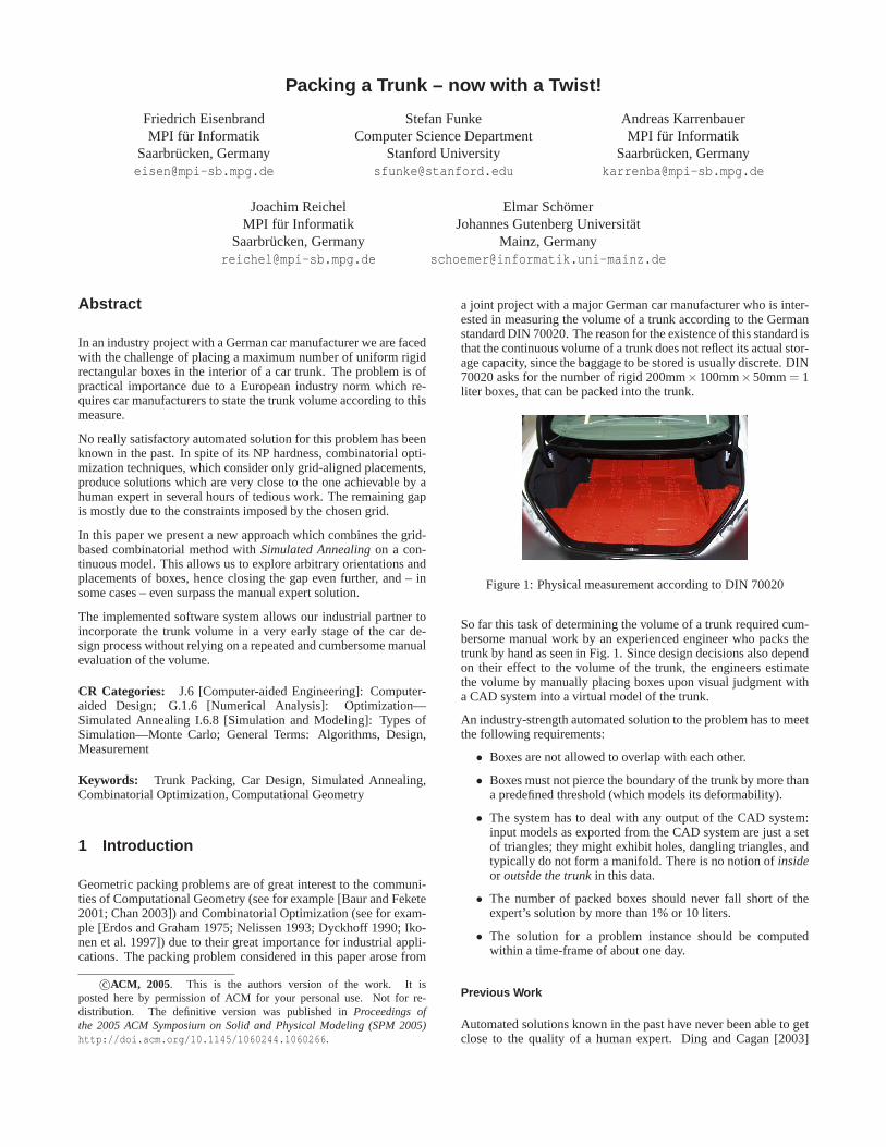
a joint project with a major German car manufacturer who is inter-ested in measuring the volume of a trunk according to the Germanstandard DIN 70020. The reason for the existence of this standard isthat the continuous volume of a trunk does not reflect its actual stor-age capacity, since the baggage to be stored is usually discrete. DIN70020 asks for the number of rigid 200mm×100mm×50mm= 1liter boxes, that can be packed into the trunk.

Figure 1: Physical measurement according to DIN 70020

So far this task of determining the volume of a trunk required cum-bersome manual work by an experienced engineer who packs thetrunk by hand as seen in Fig. 1. Since design decisions also dependon their effect to the volume of the trunk, the engineers estimatethe volume by manually placing boxes upon visual judgment witha CAD system into a virtual model of the trunk.

An industry-strength automated solution to the problem has to meetthe following requirements:

• Boxes are not allowed to overlap with each other.

• Boxes must not pierce the boundary of the trunk by more thana predefined threshold (which models its deformability).

• The system has to deal with any output of the CAD system:input models as exported from the CAD system are just a setof triangles; they might exhibit holes, dangling triangles, andtypically do not form a manifold. There is no notion ofinsideor outside the trunkin this data.

• The number of packed boxes should never fall short of theexpert’s solution by more than 1% or 10 liters.

• The solution for a problem instance should be computedwithin a time-frame of about one day.

Previous Work

Automated solutions known in the past have never been able to getclose to the quality of a human expert. Ding and Cagan [2003]

published an approach that is suited for the Society of AutomotiveEngineers (SAE) standard used in the USA. This standard differssignificantly from the European norm. It defines a luggage set con-sisting of objects varying from 6 to 67 liters. Therefore, our soft-ware has to handle far more objects than in the SAE case.

NP-Hardness of our packing problem was established in a recentresult ([Eisenbrand et al. 2003]), but still, in the same paper a firstalmost industry-strength solution was presented that using a dis-cretization model and techniques from combinatorial optimizationproduced solutions very close to the ones achievable by a humanexpert. It only rarely fell short of the prescribed bounds for the so-lution quality, which was due to the fact that this algorithm onlyallowed axis-aligned and discrete placements of the boxes in a grid.For these “bad” problem instances – which for example arise intrunks with side-compartments holding tightly a few boxes (seeFig. 2)–, there was also no hope to obtain a better solution usingthis approach, as the discretization would have had to adapt locallyto the geometry of the trunk1.

Figure 2: Arbitrary placement necessary in side-compartments nextto the wheelhouse

On the theory side, results in this area have been rather discourag-ing. [Fowler et al. 1981] have shown that already the 2-dimensionalproblem of packing axis-parallel unit squares into a polygon withholes is NP-complete, even though approximation schemes areavailable [Hochbaum and Maass 1985]. For polygons withoutholes, it is conjectured ([Baur and Fekete 2001]) that the problemis polynomially solvable. The more general problem of packing(a×b) axis-aligned rectangles inside a polygon, is not even knownto be in NP, partly because the representation of an optimum solu-tion might be arbitrarily complex (see [Nelissen 1993] for a elabora-tion on the topic). The ’Open Problem Project’ website ([Demaineet al. 2005a; Demaine et al. 2005b], problems 55, 56) keeps trackof the current status of these problems.

Our Contribution

In this paper we overcome the weakness of the previous algorithmand present an industry-strength solution to the trunk packing prob-lem which almost always comes very close to the manual solutionand in some cases even surpasses it. This breakthrough is achievedby allowingarbitrary orientation and placements of the boxes, notrestricting to axis-aligned placements on a grid as in the algorithmfrom [Eisenbrand et al. 2003].

Allowing such a continuous model leads to a very high-dimensionalglobal optimization problem for which standard methods likeSim-ulated Annealing[Kirkpatrick et al. 1983] are typically used. Un-fortunately, applying these techniques in a straightforward manneryields solutions far worse than the discretization algorithm. Onlyby combining both techniques we were able to obtain the industry-strength system.

1These pathological instances were discovered when evaluating the sys-tem from [Eisenbrand et al. 2003] in the industrial production environment.

This paper elaborates on the details of the synthesis of both meth-ods. Roughly speaking, we were able to eliminate the heating pro-cess typical for a simulated annealing procedure by using a solutionfrom the discretization algorithm as a starting configuration. Fur-thermore we devised special procedures for creation of new boxes,a relaxation by a Monte Carlo simulation, and pruning of undesiredboxes. Due to physical analogies, we call our methodSpecializedGrand Canonical Simulated Annealing.

The resulting software system meets all requirements of our indus-trial partner and is currently being installed for use in the actualdesign process of new cars.

2 Modeling the Problem

We are provided with the digital data of the car trunk by a set of tri-angles exported from a free-form CAD system. Since the originalmodel in the CAD system often consists of many parts which arenot necessarily tightly joined, the resulting set of output trianglesneither bound a closed volume nor do they form a manifold. This’low quality’ of the input data requires additional care in the pro-cessing of our algorithms. In the following section we will presenttwo ways to model the trunk packing problem such that optimiza-tion techniques can be successfully applied.

2.1 Discretizing Space and Box Orientations – a Com-binatorial Approach

The approach used in [Eisenbrand et al. 2003] proposes a dis-cretization of space and box orientations by constructing a three-dimensional cubic grid which approximates the interior of thetrunk. Boxes can only be placed anchored at a grid cube and inalignment with the grid axes, so the placement of a box is deter-mined by six parameters: the anchor cube with coordinates(x,y,z),and the orientation(w,h,d) which describe the extension of the boxin width, height and depth (measured in unit cubes). The spacingw of the cubic grid is chosen such thatk · w = 50mm for some inte-gerk, and hence the orientation(w,h,d) can be any permutation ofthe set{1k,2k,4k}. As the following stages are very sensitive to a“good” initial placement and orientation of the cubic grid, the latteris chosen such that the number of cubes contained in the interior ofthe original trunk volume is maximized. See Fig. 3 for an example.

Figure 3: Cubic grid approximating the interior of a trunk

The slightly modified goal is now to place as many boxes in thecubic grid such that each box consists only of cubes approximat-ing the interior of the trunk, and no two boxes share a cube. Thisproblem can be formalized using the following construction: LetG(V,E) be the graph with node setV and edge setE. There is anodevx,y,z,w,h,d ∈V iff the box anchored at(x,y,z) and orientation(w,h,d) consists only of cubes in the interior of the trunk. Thereis an edgee= (v,w) ∈ E iff the two corresponding box placementsof v and w intersect, i.e. share a common cube.G is called theconflict graph. Packing the largest number of boxes in the cubicgrid is then equivalent to determining themaximum independentormaximum stableset in the conflict graphG.

In [Eisenbrand et al. 2003], several techniques from integer linearprogramming and combinatorial optimization were applied to solvethis stable set problem. This approach produced packings whichmost of the time were sufficiently close to the prescribed qual-ity bound of our industrial partner. Though, when evaluating thissystem in the industrial production environment, some instancesshowed up, where the results were not satisfactory.

The inherent problem of this approach is that it chooses right at thebeginning a discretization of space and orientations which mightnot accommodate to the local geometry of the trunk. While somechoice of the grid axes might be suitable for most regions of thetrunk (e.g. typically it is reasonable to have two grid axes parallelto the bottom of the trunk), there are areas where a different orien-tation is necessary if no space should be wasted. This happens inparticular along curved parts of a trunk, see for example in Fig. 4,where the restriction to one cubical grid system wastes a lot of vol-ume along the curved lid (left picture) compared to a solution witharbitrary rotations (right picture).

Figure 4: Curved lid

Similar difficulties arise in trunks with side compartments whichtightly hold a few boxes. If the grid is not aligned with these places,volume is wasted, see also Fig. 2.

2.2 Arbitrary Placement of Boxes – a Simulated Anneal-ing Approach

To overcome the problems with these pathological cases, we haveto extend our model to account for arbitrary positions and orienta-tions of the boxes. In such a model the placement of a box can becharacterized by a 6-tuple(x,y,z,θ ,ϕ ,ψ) ∈ R

6 (not Z6 as in the

discrete model). We are interested in a collection ofn such 6-tuplessuch that their corresponding box placements do not overlap andare completely contained in the interior of the trunk. The valuenshould be as large as possible such that a valid placement still exists.

Let us first focus on the case wheren is fixed, and we are only look-ing for a valid placement ofn boxes. This 6n-dimensional problemis far too complicated to be solved using techniques from convexoptimization, hence generic optimization techniques likeSimulatedAnnealing (SA)are the method of choice. This technique can be

implemented by designing a suitablepotentialor energy functionU : R

6n → R+0 from possible configurations, i.e. placements of the

n boxes, to the real numbers. Valid configurations should result ina low potential or energy value whereas invalid configurations dueto overlap or non-containment in the trunk should be assigned highpotential values. The goal is to find a global minimum (also calledground state) of this potential functionU . The approach of SA isto define transitions from one configuration to another and then ba-sically start a random walk on the implicitly defined (potentiallyinfinite) graph. At the beginning, at “high temperature”, transitionsmight happen even to configurations with a higher energy value,but with decreasing temperature, configurations of lower energy arepreferred. In our solution we enhance the basic SA approach witha method for growing and shrinking the size of a configuration (i.e.the valuen).

Both, a suitable definition of a potential function for our problemas well as some extensions to the basic SA process will be the topicof the rest of this paper. The latter extensions were crucial for ob-taining solutions superior to the discretization approach.

3 Simulated Annealing – Potential Functionand Basics

In this section we will derive a potential function for the trunk pack-ing problem, give a brief overview of the employed simulated an-nealing process and provide some details about an efficient evalua-tion procedure for the potential function.

3.1 The Potential Function

It is natural to split the potential into two parts. On one hand wehave the penetration of the exterior that we measure by the so calledwall potential UW. On the other hand we have a contribution frompairwise interaction of the boxes. The interaction term consists oftheintersection volume UV and theinterpenetration depth UI of twoboxes. We define our potential as a convex combination of thesethree parts. Letx = (x1, . . . ,xn) be the coordinates of a configura-tion wherexi is the set of the coordinates for boxi. Then, we havefor the potential

U(x) = λW

n

∑i=1

UW(xi)+λV

n

∑i=1

i−1

∑j=1

UV(xi ,x j )+λI

n

∑i=1

i−1

∑j=1

UI (xi ,x j ),

whereλW,λV ,λI ≥ 0 are the respective weights for the three contri-butions. The conditionλW +λV +λI = 1 for the convexity ensuresthat we do not effectively change the temperature of the system byreweighting the contributions during the algorithm.

In the next paragraph we develop the contribution of the pairwisebox interaction to the potential. For the sake of simplicity, we re-strict ourselves to the two-dimensional case. The extension to threedimensions should be straight forward.

Interaction Given two boxes by the open setsBi ,B j defined bytheir coordinatesxi ,x j for position and orientation, we define theintersection volume UV as

UV(xi ,x j ) =∫

Bi∩B j

dV.

Using only the intersection volumeUV and neglecting the interpen-etration depthUI in the potential would be sufficient in theory. But

the overlap is not qualified very intuitively in some exceptional sit-uations. Therefore we do not only consider the intersection volume,but also the penetration depth of two boxes.

b

ε ϕ

Figure 5: Motivation for penetration depth

Consider two rectangles that touch at an edge with lengthb. Ifwe now push the rectangles into one another byε orthogonallyto that edge, we get an overlapUV = b · ε as depicted in Fig. 5.Now assume that the two rectangles touch by an edge and a ver-tex. The overlap that results from a penetration ofε is given byUV = ε2

sin2ϕ . Sinceε ≪ b the overlap resulting from the same pen-etration is much smaller in the second case opposing our intuition.Therefore, we define an additional measure that is more adequatein such situations.Definition 1. Given a metric space(X, |·|), the penetration depthof two open sets A,B⊂ X is defined as

min{|t| : A∩ (t +B) = /0, t ∈ X}.

Informally speaking, the penetration depth is the distance that oneobject needs to be translated in order to dissolve the intersection.We set theinterpenetration depth UI (xi ,x j ) of two boxes to theirpenetration depth and get a further contribution to the potential inaddition to the intersection volumeUV . We cannot simply replaceUV by UI because the latter has also its drawbacks. Consider theleft situation depicted in Fig. 5. The penetration depth is the smallvertical distanceε. If the rectangles are blocked in that direction,i.e. that vertical moves are not permitted by the boundary or otherrectangles, then the only way to reduce the overlap is by movinghorizontally. But for a great deal of horizontal moves the potentiallooks the same with respect to the penetration depth, namelyε andthus involving a lot of iterations to get out.

Wall Potential In two-dimensional packing problems one oftenhas a polygon that defines the container. There it is possible totake its complement and treat it like an obstacle. In that case thepenetration depth of the boxes with the boundary is well defined.

But this does not hold in our particular case. The data of the trunk isgiven as a triangular mesh with a penetration thresholdpT for eachtriangle. We may not assume any further properties on the mesh,e.g. that it is a manifold, watertight or that the normals are orientedconsistently.

Though, we can use the principle of the penetration depth similar tothe two dimensional case, but we must adjust it to our setting. Thepenetration depth for each box is defined per triangle instead of thewhole body. Thereby, it is also possible to treat certain regions

differently, e.g. the bottom of a trunk would hardly give way incontrast to the sides where a few millimeters are always acceptable.

This introduces some problems with respect to the total potential.We cannot just sum up the values for each triangle since then thevalue would increase if the boundary is triangulated finer. There-fore, we use the maximum of all triangles. It is also possible to usethe mean of all positive contributions.

The penetration depth for a triangle with respect to a given box isalso defined as the minimum distance to pull it apart from that box.

Thereby, the wall-potential is positive only for those boxes touchingthe boundary. But this is definitely not what we want for boxeslocated completely outside.

pR

p

pT

UW

outsideinside boundary

Figure 6: Wall potential of a box moving through the boundary

It is even more counter-intuitive if we think of a box moving fromthe inside to the outside like illustrated in Fig. 6. Its potential in-creases to a maximum attained when the center crosses the bound-ary and then decreases symmetrically to zero again until it does nottouch the trunk anymore.

Therefore, we define therestricted penetration depth pR that onlyconsiders translations that would move the box back inside thetrunk. Hence, we have to define what is inside and outside withrespect to the trunk in a way we can use it for computation. Butas pointed out earlier, there is an ambiguity in the representation ofthe trunk since we cannot expect the model to be watertight.

Thus, the restricted penetrationpR is infeasible to compute. Butsince it coincides with the penetration depthp in certain regions,we just use the latter and ensure that we report “infinity” in case ofp < pR.

We define thewall potential UW in terms of a predicate that tellsus whether a box should be treated as outside the trunk and use themaximal penetration depth otherwise, i.e.

UW(xi) =

{∞ if outside(xi)

max{p(xi ,τ) : τ ∈ Triangles} otherwise,

wherep(xi ,τ) is the minimum distance that the triangleτ has to betranslated such that it does not intersect the box. We must designtheoutside predicate very carefully such that it is robust but nev-ertheless efficient to evaluate. This issue is addressed in Sect. 4.3

Observe that the contribution of a particular box to the potentialhas a short range, i.e. it is completely determined by objects inthe neighborhood. We can benefit from this when evaluating thepotential.

3.2 Monte Carlo algorithm

In 1953, Metropolis et al. introduced the Monte Carlo importance-sampling algorithm [Metropolis et al. 1953]. It’s a method that isused in statistical physics to predict or check macroscopic proper-ties of complex, i.e. many-body, systems that result from an as-sumed potential.

In nature, realizations with different energies of such a statisticalensemble do not appear with the same probability. The configura-tions that lead to a lower potential energy are much more likely tooccur. In our case we consider the Boltzmann distribution that sug-gest a probability for a configuration with potential energyU that isproportional toe−βU whereβ is the inverse temperature. We treatβ simply as a parameter and only refer to its physical meaning toget an intuition.

Since it is infeasible to enumerate all configurations, we try to limitthe evaluations of the potential to important configurations. Given astarting configuration, we want to “walk” through the configurationspace guided by our potential. Therefore, we propose trial movesthat are accepted depending on the change in the potential. If theproposed configuration has a lower energy we accept it with prob-ability 1. Otherwise, we accept it with a probabilityp = e−β ·∆U

where∆U is positive. This scheme is depicted in Fig. 7.

evaluatePotentialU1

- trial move - evaluatePotentialU2

-else

��

��

��3

p = e−β ·∆U

accept

-else

reject

?

∆U = U2−U1 > 0

oracle

Figure 7: Metropolis Monte Carlo Scheme

It is absolutely necessary to take steps that preliminary lead to ahigher energy in order to escape from local minima. This behavioris controlled by the parameterβ . The higher its value is the moreunlikely is the worsening in terms of the potential energy.

Since the boxes in the middle are much less flexible than the boxesat the boundary, each box has its own range from that we chooseour trial moves. We dynamically adapt these ranges by increasingit if a move is accepted and decreasing it otherwise. Thereby, weachieve that the acceptance settles down at 50 %.

Since the potential seen by a box does not look like the same inevery direction, we do not adjust the ranges for all coordinates inthe same way. We rather distribute the amount of the change to thecoordinates with respect to the suggested trial move.

We do not move all boxes simultaneously but one randomly pickedin each iteration.

3.3 Evaluating the Potential Function efficiently

This is the most time-consuming task in our algorithm. Profiling ex-periments have shown that more than 90 percent of the CPU-time isspent in the routines for the computation of the intersection volumeand the penetration depth. Again, we consider the two dimensionalcase to illustrate the idea.

First, we describe a method that decides whether two rectanglesoverlap. Afterwards we slightly modify that procedure by addinglittle costs so that it also tells us the penetration depth. At the endof this section, we illustrate how to compute the overlapping area.

It can be easily shown that the definition of the penetration depth isequivalent to

min{|~t| :~t ∈ A⊕ (−B)},i.e. in the complement of the Minkowski sum of both sets. Actually,we do not compute any Minkowski sums here but use this techniqueto prove the correctness of our approach.

By the definition of the penetration-depth of two rectanglesRi andRj , the minimum is attained at the borderB of the setRi ⊕ (−Rj)which is determined by at most eight constraints that are parallel tothe sides of the two rectangles as seen in Fig. 8.

$R_i$

$R_j$$\vec{t}$

$R_I \oplus (−R_j)$

Ri

Rj

~t

B

Figure 8: Determining the penetration depth

Since we consider the penetration depth with respect to the Eu-clidean distance, it coincides with the radius of the maximal circlecentered at the origin that fits intoB.

By elementary geometry the vector pointing from the origin to theboundary point is perpendicular to the corresponding face. Hence,the direction of a translation that determines the penetration depthis a normal of one of the faces that defineB.

By the separating axis theorem for convex polyhedra [Gottschalket al. 1996], these normals are either the ones of the two polyhedraor are parallel to the cross product of an edge of the first polyhe-dron and an edge of the second one. Since we consider rectanglesin 2D those normals are exactly the directions of the edges of therectangles.

Ri

Rj

Figure 9: Separating axis

We consider the projections of the objects on one of those directionsnow. Hence, we have two intervals each corresponding to one of thepolyhedra. The separating axis theorem tells us further that the twopolyhedra are disjoint iff for at least one of those directions the twointervals are disjoint.

Thus, we have a test that tells us two rectangles apart. In the worstcase it requires to test four directions since at least half of the eight

edges are parallel. As soon as we get two disjoint intervals we aredone and report that there is no overlap or the penetration depth iszero respectively.

Furthermore, we can modify this test slightly in order to get amethod that computes the penetration depth directly at not muchmore cost. Assume we test in directionk = 1, . . . ,4 and observe anoverlap oftk of the intervals that result from the projection.

Without loss of generality, we may assume thattk is positive sinceotherwise we swap the roles of the rectangles. We construct a trans-lation~tk with |~tk| = tk pointing in the direction of the projection.

~t

Rj

Ri

Figure 10: Penetration depth by projection

If we translate the corresponding rectangle by~tk the two rectanglesbecome disjoint because then we can place a separating hyperplanewith normal~tk between them. Recall that the value for the penetra-tion depth is attained by a vector that points into one of the testeddirection. Thus, we simply report the minimum absolute value ofall thosetk.

Intersection volume of two boxes Since boxes are convex poly-hedra their intersection can be simply computed by solving a halfs-pace intersection problem. In general the intersection body consistsof trimmed facets originating from both boxes. In order to findthese trimmed facets, we triangulate the boundary of every box andclip its triangles by the three pairs of parallel planes defining theother box. Clipping a triangle by a plane may produce a quadranglewhich we decompose into two triangles for further clipping. Thisbasic geometric operation can be implemented very easily and re-sults in a highly specialized and effective routine for determininga setT of oriented triangles which form the boundary of the in-tersection body. Connectivity information among these triangles isnot required for computing the desired volume: Let∆ = (~a∆,~b∆,~c∆)denote an oriented triangle ofT then the volumeV is given by

V =16 ∑

∆∈T

∣∣∣∣1 1 1 1~o ~a∆ ~b∆ ~c∆

∣∣∣∣ ,

where~o is an arbitrary fixed reference point.

Because of the short range of interaction, only boxes in the directneighborhood of a moving box constitute to its intersection volumeand penetration depth. That is why we use a uniform grid as a spacepartitioning scheme to locate all potentially interfering boxes andpenetrated boundary triangles. The relatively expensive computa-tion of the intersection volume for two boxes is only executed if thefast disjointness test (based on the separating axes theorem) fails.In this way we succeed in performing thousands of trial moves persecond in the Monte Carlo simulation.

Figure 11: Intersection figure by iterative clipping

4 Simulated Annealing – The Efficient Imple-mentation

This section is dedicated to our extensions and modifications of thesimulated annealing approach. At the beginning, we take a com-binatorial solution from the discrete model to eliminate the heatingprocess, i.e. we avoid to equilibrate the system at a very high tem-perature leading to strongly disordered configurations. This issue isdescribed in Sect. 4.5 in more detail.

In our algorithm, we iteratively apply a sequence consisting of

• a special creation procedure for new boxes,

• a relaxation period by a Monte Carlo simulation, and

• a randomly triggered destruction of the “worst” box.

Before we explain the special creation procedure and the destruc-tion of boxes in Sect. 4.4, we give some implementation detailsthat are necessary for an efficient simulation. During the relaxationperiod, we select with probability of12 between translational androtational moves.

4.1 Translational Trial Moves

Let ∆x,∆y,∆z be three parameters defining the range

R= (−∆x,∆x)× (−∆y,∆y)× (−∆z,∆z)

from which the displacements~t 6= 0 for the trial moves are pickeduniformly at random. We do nothing in the stationary case becauseit gets trivially accepted and does not give any useful information.The potential change∆U is given by

∆U = U(~r +~t)−U(~r),

where~r is the old position and~t ∈ R the displacement of the box.Now we consider the two cases “Accepted” and “Rejected” sepa-rately.

Accepted In the case of an accepted trial move, we update theposition of the box and increase the parameters∆x,∆y and∆z bymultiplying by a factor of 1+ |tx|/|~t|, 1+ |ty|/|~t| and 1+ |tz|/|~t|respectively.

Rejected If the trial move is rejected, we discard the trial moveand decrease the parameters∆x,∆y and∆z by division by a factorof 1+ |tx|/|~t|, 1+ |ty|/|~t| and 1+ |tz|/|~t| respectively.

4.2 Rotational Trial Moves

We choose quaternions as representation for orientations and ro-tations instead of the Eulerian anglesθ ,ϕ ,ψ because they easilyallow choosing rotations uniformly at random. For this purpose,we consider the interpretation

q = (cosϑ ,~u·sinϑ)

which is a rotation by an angle 2ϑ about an axis represented by theunit vector~u.

We pick a point uniformly distributed in the three dimensional unitball by choosing three independent uniformly distributed randomnumbersp1, p2, p3 ∈ [0,1) and rejecting every triple withp2 :=p2

1 + p22 + p2

3 ≥ 1. Then we generate a quaternion

δq =1√

1+ p2(1, p1, p2, p3)

which defines a rotation about a uniformly distributed axis.Whereas,ϑ ∈ [0, π

4 ) covers rotations between zero and 2·45= 90degrees. By scaling the vector~p we can control the magnitude ofthe rotation, too.

Given a trial rotationδq∈ R4, the potential change∆U is given by

∆U = U(q·δq)−U(q),

whereq∈ R4 is the old orientation. Similar to the case of transla-

tional moves we maintain parameters∆1,∆2,∆3 to scale the com-ponents of~p. Thereby, we effectively choose the rotational axis outof an ellipsoid instead of a ball.

4.3 Prevention of Boxes from Escaping

As we have seen in Sect. 2.2, the penetration depthp does not suf-fice to model the wall potential. We are interested in the restrictedpenetration depthpR, but cannot compute this value due to the de-ficiencies of the representation of the trunk. Actually, it suffices todistinguish the casesp = pR ≤ 1

2 lmin andp < 12 lmin < pR in Fig. 6

wherelmin is the shortest side length of a box. In the following wedescribe an approach to overcome this problem.

The goal is to develop a predicate calledoutside(~c), that reflectsthe position of a box with center~c with respect to the trunk. Thepredicate should returnfalse for boxes completely contained inthe trunk or for boxes with small restricted penetration depth. If therestricted penetration depth exceeds a certain threshold, the predi-cate should returntrue. This predicate is used to distinguish bothcases in the definition of the wall potentialUW.

We use a three-dimensional grid that segments the bounding box ofthe trunk into cells. The purpose of the grid is to approximate thespace with respect to the trunk. Each grid cell belongs to exactlyone of three sets, namelyinterior, boundaryandexterior cells. Thespacingd of the grid is discussed later.

The set of boundary cells can be easily determined by computingthe intersections between grid cells and the triangular mesh of thetrunk. Next we want to identify the interior and exterior cells. Wecompute connected components of grid cells not yet identified asboundary cells. For this computation, cells are viewed as nodes ofa graph and cells next to each other are handled as adjacent nodes.

In order to ensure that regions in the interior and exterior of thetrunk do not end up in the same component, we demand that theholes in the triangular mesh do not exceed a rectangle of sized×d.

All cells of the connected component(s) that contain(s) the outmostlayer of the grid cells clearly belong to the outside (or boundary)and are marked as such.

Since our model is not a manifold we might still have two or morecomponents not yet assigned to one of the tree sets. Therefore werequire the user to specify one point in the interior of the trunk. Thecells in the corresponding component are marked as inside, all otherremaining components (if any) are marked as outside.

Given this data structure, we implement the predicateoutside(~c)as follows. We returntrue if the center~c is not contained in thebounding box. Otherwise, we look up the grid cell corresponding tothe query point~c and returntrue iff the cell is marked as boundaryor outside.

What remains to be discussed is the choice of the spacing parame-terd and its influence on the predicate with respect to the restrictedpenetration depth of a box. This relation is established by the fol-lowing proposition.Proposition 1. Given a grid with spacing d> 0 and a box withcenter~c and minimum side length lmin. If outside(~c) returnstrue, we have for the the restricted penetration depth pR

pR ≥ 12

lmin−d√

3.

Proof. Consider the case that the cell corresponding to the center~cis marked as boundary (see Fig. 12). The distance between~c andthe boundary is at most the diagonal of the cell, which isd

√3. Thus

the restricted penetration depth is at least12 lmin−d

√3.

lmin/2

d

outside

inside~c

≤ d√

3

pR

boundary

Figure 12: Box center lies in boundary cell

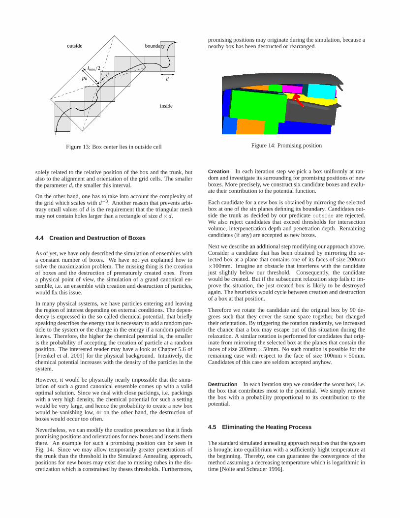
Now consider the case that the cell of the center~c is marked asoutside (see Fig. 13). The restricted penetration depthpR is greateror equal than the distance of the center~c to the boundary of the box,hencepR ≥ 1

2 lmin.

The case that the center~c is not contained in the bounding boxcan be handled as the second case for a grid augmented with oneadditional outmost layer of cubes marked as outside.

The contraposition yields that our predicate reportsfalse forpR < 1

2 lmin− d√

3. Additionally, the predicate returnstrue forpR > 1

2 lmin (since the center of such a box lies in a cell marked asboundary or outside). Hence the spacing parameterd adjusts theinterval of “uncertainty” in which the result of the predicate is not

d

outside

pR

lmin/2

inside

boundary

~c

Figure 13: Box center lies in outside cell

solely related to the relative position of the box and the trunk, butalso to the alignment and orientation of the grid cells. The smallerthe parameterd, the smaller this interval.

On the other hand, one has to take into account the complexity ofthe grid which scales withd−3. Another reason that prevents arbi-trary small values ofd is the requirement that the triangular meshmay not contain holes larger than a rectangle of sized×d.

4.4 Creation and Destruction of Boxes

As of yet, we have only described the simulation of ensembles witha constant number of boxes. We have not yet explained how tosolve the maximization problem. The missing thing is the creationof boxes and the destruction of prematurely created ones. Froma physical point of view, the simulation of a grand canonical en-semble, i.e. an ensemble with creation and destruction of particles,would fix this issue.

In many physical systems, we have particles entering and leavingthe region of interest depending on external conditions. The depen-dency is expressed in the so called chemical potential, that brieflyspeaking describes the energy that is necessary to add a random par-ticle to the system or the change in the energy if a random particleleaves. Therefore, the higher the chemical potential is, the smalleris the probability of accepting the creation of particle at a randomposition. The interested reader may have a look at Chapter 5.6 of[Frenkel et al. 2001] for the physical background. Intuitively, thechemical potential increases with the density of the particles in thesystem.

However, it would be physically nearly impossible that the simu-lation of such a grand canonical ensemble comes up with a validoptimal solution. Since we deal with close packings, i.e. packingswith a very high density, the chemical potential for such a settingwould be very large, and hence the probability to create a new boxwould be vanishing low, or on the other hand, the destruction ofboxes would occur too often.

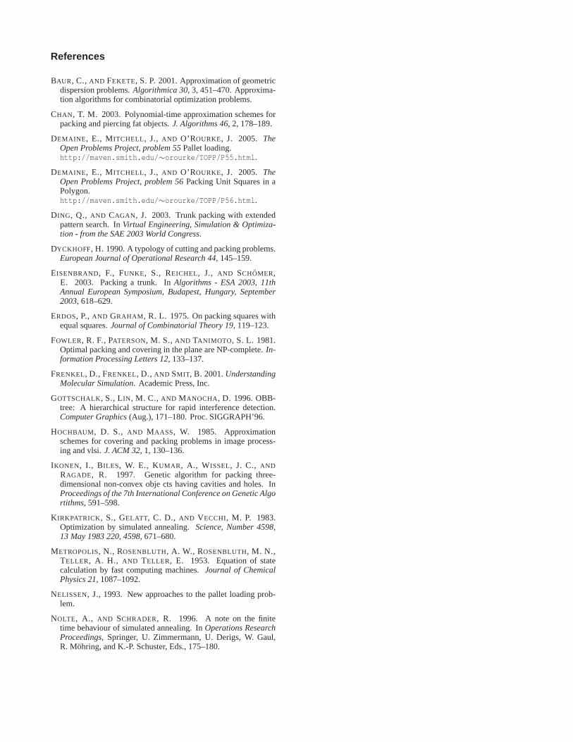
Nevertheless, we can modify the creation procedure so that it findspromising positions and orientations for new boxes and inserts themthere. An example for such a promising position can be seen inFig. 14. Since we may allow temporarily greater penetrations ofthe trunk than the threshold in the Simulated Annealing approach,positions for new boxes may exist due to missing cubes in the dis-cretization which is constrained by theses thresholds. Furthermore,

promising positions may originate during the simulation, because anearby box has been destructed or rearranged.

Figure 14: Promising position

Creation In each iteration step we pick a box uniformly at ran-dom and investigate its surrounding for promising positions of newboxes. More precisely, we construct six candidate boxes and evalu-ate their contribution to the potential function.

Each candidate for a new box is obtained by mirroring the selectedbox at one of the six planes defining its boundary. Candidates out-side the trunk as decided by our predicateoutside are rejected.We also reject candidates that exceed thresholds for intersectionvolume, interpenetration depth and penetration depth. Remainingcandidates (if any) are accepted as new boxes.

Next we describe an additional step modifying our approach above.Consider a candidate that has been obtained by mirroring the se-lected box at a plane that contains one of its faces of size 200mm×100mm. Imagine an obstacle that interferes with the candidatejust slightly below our threshold. Consequently, the candidatewould be created. But if the subsequent relaxation step fails to im-prove the situation, the just created box is likely to be destroyedagain. The heuristics would cycle between creation and destructionof a box at that position.

Therefore we rotate the candidate and the original box by 90 de-grees such that they cover the same space together, but changedtheir orientation. By triggering the rotation randomly, we increasedthe chance that a box may escape out of this situation during therelaxation. A similar rotation is performed for candidates that orig-inate from mirroring the selected box at the planes that contain thefaces of size 200mm×50mm. No such rotation is possible for theremaining case with respect to the face of size 100mm× 50mm.Candidates of this case are seldom accepted anyhow.

Destruction In each iteration step we consider the worst box, i.e.the box that contributes most to the potential. We simply removethe box with a probability proportional to its contribution to thepotential.

4.5 Eliminating the Heating Process

The standard simulated annealing approach requires that the systemis brought into equilibrium with a sufficiently hight temperature atthe beginning. Thereby, one can guarantee the convergence of themethod assuming a decreasing temperature which is logarithmic intime [Nolte and Schrader 1996].

Since this implies an exponential running time, one has to use fasterschedules, e.g. a geometric one. But thereby, we experienced lotsof canting of the boxes like depicted in Fig. 15.

Figure 15: Canting of boxes

Therefore, we came up with the idea to use a combinatorial solutionas starting configuration in connection with our creation procedure.In the following, we give a model of the configuration space thatexplains the success of our method.

Lets assume that we only have uniform objects to pack like in ourreal world problem. Therefore, the potential does not change byswapping the identity of two boxes. Hence, it is sufficient to con-sider only one representative configurationx = (s1, . . . ,sn) for allits n! permutations wheren is the number of boxes andsi the set ofparameters that describe one box.

If we consider the statessi ,sj of two boxes in a common subspace,then their “distance” cannot be arbitrarily close in a valid packing.Therefore, we may assume that each state occupies a certain volumeof the configuration space. Since we are interested in a maximalpacking, i.e. a packing with a high density of states, an optimalsolution would be a close packing.

optimal solutionstarting config

occupied space

Figure 16: Model of states in the configuration space

Our heuristics consists of choosing a starting configuration in away that yields a closest packing because thereby we can map eachstate of the starting configuration to one state of an optimal solutionsuch that each distance is bounded. Therefore, an appropriate start-ing configuration would be a combinatorial solution to the discretemodel with the additional constraint that it is dense in its interior.

Since the starting configuration is “near” an optimal solution butdoes not match exactly, we have an additional requirement that thecombinatorial solution should be “flexible” enough, i.e. rather ho-mogeneous in the orientation of the boxes.

Note that we still follow a cooling schedule in the course of our al-gorithm. But by using the combinatorial solution, we are allowed tostart at a lower temperature that does not lead to a randomization ofthe whole starting configuration and the related canting problems.

5 Project Overview and Evaluation

The complete project has been implemented in C++ and is portableacross today’s major system platforms. Several external librarieshave been used supporting the implementation of the user inter-face, the visualization part as well as providing some low-level al-gorithms and datastructures. Since our system is employed in anindustrial production environment, ease-of-use has been a major re-quirement of our industrial partner.

5.1 Evaluation

Here we briefly report on the results we achieved with our approachof theSpecialized Grand Canonical Simulated Annealingheuristic.

The plain results are summarized in Tab. 1 where we oppose the val-ues achieved by a human expert, our best combinatoric solutions,and the novel approach which is abbreviated by SGCSA. Just to getan impression, we also added an approximate value for the continu-ous volume in the last column. This value is the average of an innerand outer approximation by a cubic grid with a spacing of 6.25 mmor 12.5 mm and has been rounded to a precision of 5 liters.

A, B, C, and D denote different trunk types, ’C w/ extras’ the sametrunk as C but with a reduced volume due to control units for addi-tional equipment like air-conditioning.

expert combinatoric SGCSA continuousA 62 l 61 l 64 l ≈95 lB 80 l 80 l 81 l ≈120 lC 513 l 507 l 510 l ≈595 lC w/ extras 480 l 475 l 479 l ≈555 lD 499 l 491 l 493 l ≈595 l

Table 1: Some test cases

Recall that the quality restrictions of our industrial partner requireus to achieve least 99% of their best manual packing and not morethan 10 liters less. One can see in Tab. 1 that for modelsA andB,our implementation even outperforms the expert’s solution. All so-lutions were computed within a time-frame of one day allowed byour industrial partner; since no user interaction is required after ini-tializing the optimization process, this fits very well into the designprocess.

6 Conclusion

We have presented an industrial-strength system which enables carmanufacturers to estimate reliably the volume of car trunks evenat an early stage of the design process. Compared to the previ-ous system presented in [Eisenbrand et al. 2003], the main noveltyis the possibility to place boxes in arbitrary orientations and posi-tions. The lack of the latter has shown to be a weakness of the oldsystem when it was evaluated in the actual production environment.The new system has been certified using a large number of differenttrunk types and proven to be of industrial strength. It is currentlybeing installed for use in the actual design process of the car manu-facturer.

References

BAUR, C., AND FEKETE, S. P. 2001. Approximation of geometricdispersion problems.Algorithmica 30, 3, 451–470. Approxima-tion algorithms for combinatorial optimization problems.

CHAN , T. M. 2003. Polynomial-time approximation schemes forpacking and piercing fat objects.J. Algorithms 46, 2, 178–189.

DEMAINE , E., MITCHELL , J., AND O’ROURKE, J. 2005. TheOpen Problems Project, problem 55Pallet loading.http://maven.smith.edu/∼orourke/TOPP/P55.html.

DEMAINE , E., MITCHELL , J., AND O’ROURKE, J. 2005. TheOpen Problems Project, problem 56Packing Unit Squares in aPolygon.http://maven.smith.edu/∼orourke/TOPP/P56.html.

DING, Q., AND CAGAN , J. 2003. Trunk packing with extendedpattern search. InVirtual Engineering, Simulation & Optimiza-tion - from the SAE 2003 World Congress.

DYCKHOFF, H. 1990. A typology of cutting and packing problems.European Journal of Operational Research 44, 145–159.

EISENBRAND, F., FUNKE, S., REICHEL, J., AND SCHOMER,E. 2003. Packing a trunk. InAlgorithms - ESA 2003, 11thAnnual European Symposium, Budapest, Hungary, September2003, 618–629.

ERDOS, P.,AND GRAHAM , R. L. 1975. On packing squares withequal squares.Journal of Combinatorial Theory 19, 119–123.

FOWLER, R. F., PATERSON, M. S.,AND TANIMOTO , S. L. 1981.Optimal packing and covering in the plane are NP-complete.In-formation Processing Letters 12, 133–137.

FRENKEL, D., FRENKEL, D., AND SMIT, B. 2001.UnderstandingMolecular Simulation. Academic Press, Inc.

GOTTSCHALK, S., LIN , M. C., AND MANOCHA, D. 1996. OBB-tree: A hierarchical structure for rapid interference detection.Computer Graphics(Aug.), 171–180. Proc. SIGGRAPH’96.

HOCHBAUM, D. S., AND MAASS, W. 1985. Approximationschemes for covering and packing problems in image process-ing and vlsi.J. ACM 32, 1, 130–136.

IKONEN, I., BILES, W. E., KUMAR , A., WISSEL, J. C., ANDRAGADE, R. 1997. Genetic algorithm for packing three-dimensional non-convex obje cts having cavities and holes. InProceedings of the 7th International Conference on Genetic Algortithms, 591–598.

K IRKPATRICK, S., GELATT, C. D., AND VECCHI, M. P. 1983.Optimization by simulated annealing.Science, Number 4598,13 May 1983 220, 4598, 671–680.

METROPOLIS, N., ROSENBLUTH, A. W., ROSENBLUTH, M. N.,TELLER, A. H., AND TELLER, E. 1953. Equation of statecalculation by fast computing machines.Journal of ChemicalPhysics 21, 1087–1092.

NELISSEN, J., 1993. New approaches to the pallet loading prob-lem.

NOLTE, A., AND SCHRADER, R. 1996. A note on the finitetime behaviour of simulated annealing. InOperations ResearchProceedings, Springer, U. Zimmermann, U. Derigs, W. Gaul,R. Mohring, and K.-P. Schuster, Eds., 175–180.