Package ‘SpATS’ - The Comprehensive R Archive Network · Package ‘SpATS’ March 6, 2018 Type...

Package ‘SpATS’May 30, 2018

Type Package

Title Spatial Analysis of Field Trials with Splines

Version 1.0-8

Date 2018-05-29

Imports stats, grDevices, graphics, fields, plot3Drgl, spam,data.table

Description Analysis of field trial experiments by modelling spatial trends using two-dimensional Penalised spline (P-spline) models.

License GPL

NeedsCompilation no

Author Maria Xose Rodriguez-Alvarez [aut, cre],Martin Boer [aut],Paul Eilers [aut],Fred van Eeuwijk [ctb]

Maintainer Maria Xose Rodriguez-Alvarez <[email protected]>

Repository CRAN

Date/Publication 2018-05-30 18:36:06 UTC

R topics documented:SpATS-package . . . . . . . . . . . . . . . . . . . . . . . . . . . . . . . . . . . . . . . 2controlSpATS . . . . . . . . . . . . . . . . . . . . . . . . . . . . . . . . . . . . . . . . 3getHeritability . . . . . . . . . . . . . . . . . . . . . . . . . . . . . . . . . . . . . . . . 4obtain.spatialtrend . . . . . . . . . . . . . . . . . . . . . . . . . . . . . . . . . . . . . . 5plot.SpATS . . . . . . . . . . . . . . . . . . . . . . . . . . . . . . . . . . . . . . . . . 7plot.variogram.SpATS . . . . . . . . . . . . . . . . . . . . . . . . . . . . . . . . . . . 8predict.SpATS . . . . . . . . . . . . . . . . . . . . . . . . . . . . . . . . . . . . . . . . 9print.SpATS . . . . . . . . . . . . . . . . . . . . . . . . . . . . . . . . . . . . . . . . . 10PSANOVA . . . . . . . . . . . . . . . . . . . . . . . . . . . . . . . . . . . . . . . . . 11SAP . . . . . . . . . . . . . . . . . . . . . . . . . . . . . . . . . . . . . . . . . . . . . 13SpATS . . . . . . . . . . . . . . . . . . . . . . . . . . . . . . . . . . . . . . . . . . . . 16summary.SpATS . . . . . . . . . . . . . . . . . . . . . . . . . . . . . . . . . . . . . . 19

1

2 SpATS-package

variogram . . . . . . . . . . . . . . . . . . . . . . . . . . . . . . . . . . . . . . . . . . 21wheatdata . . . . . . . . . . . . . . . . . . . . . . . . . . . . . . . . . . . . . . . . . . 23

Index 25

SpATS-package Spatial analysis of field trials with splines

Description

This package allows the use of two-dimensional (2D) penalised splines (P-splines) in the context ofagricultural field trials. Traditionally, the modelling of the spatial or environmental effect in the ex-pression of phenotypes has been done assuming correlated random noise (Gilmour et al, 1997). We,however, propose to model the spatial variation explicitly using 2D P-splines (Rodriguez-Alvarez etal., 2018). Besides the existence of fast and stable algorithms for estimation (Rodriguez-Alvarez etal., 2015; Lee et al., 2013), the direct and nice interpretation of the spatial trend that this approachprovides makes it attractive for the analysis of field experiments.

Details

Package: SpATSType: PackageVersion: 1.0-8Date: 2018-05-29License: GPL

Author(s)

Maria Xose Rodriguez-Alvarez, Martin Boer, Paul Eilers, Fred van Eeuwijk

Maintainer: Maria Xose Rodriguez-Alvarez <[email protected]>

References

Gilmour, A.R., Cullis, B.R., and Verbyla, A.P. (1997). Accounting for Natural and Extraneous Vari-ation in the Analysis of Field Experiments. Journal of Agricultural, Biological, and EnvironmentalStatistics, 2, 269 - 293.

Lee, D.-J., Durban, M., and Eilers, P.H.C. (2013). Efficient two-dimensional smoothing with P-spline ANOVA mixed models and nested bases. Computational Statistics and Data Analysis, 61, 22- 37.

Rodriguez-Alvarez, M.X., Lee, D.-J., Kneib, T., Durban, M., and Eilers, P.H.C. (2015). Fastsmoothing parameter separation in multidimensional generalized P-splines: the SAP algorithm.Statistics and Computing, 25, 941 - 957.

controlSpATS 3

Rodriguez-Alvarez, M.X, Boer, M.P., van Eeuwijk, F.A., and Eilers, P.H.C. (2018). Correcting forspatial heterogeneity in plant breeding experiments with P-splines. Spatial Statistics, 23, 52 - 71.https://doi.org/10.1016/j.spasta.2017.10.003.

controlSpATS Used to set various parameters controlling the fitting process

Description

This function can be used to modify some default parameters that control the estimation of anSpATS model.

Usage

controlSpATS(maxit = 200, tolerance = 0.001, monitoring = 2, update.psi = FALSE)

Arguments

maxit numerical value indicating the maximum number of iterations. Default set to200 (see Details).

tolerance numerical value indicating the tolerance for the convergence criterion. Defaultset to 0.001 (see Details).

monitoring numerical value determining the level of printing which is done during the esti-mation. The value of 0 means that no printing is produced, a value of 1 meansthat only the computing times are printed, and a value of 2 means that, at eachiteration, the (REML) deviance and the effective dimensions of the random com-ponents are printed. Default set to 2.

update.psi logical. If TRUE, the dispersion parameter of the exponential family is up-dated at each iteration of the estimation algorithm. Default is FALSE, except forfamily = gaussian(), where the dispersion parameter (or residual variance),is always updated jointly with the rest of variance components.

Details

The estimation procedure implemented in the SpATS package is an extension of the SAP (Separa-tion of anisotropic penalties) algorithm by Rodriguez - Alvarez et al. (2015). In this case, besidesthe spatial trend, modelled as a two-dimensional P-spline, the estimation algorithm allows for the in-corporation of both fixed and (sets of i.i.d) random effects on the (generalised) linear mixed model.For Gaussian response variables, the algorithm is an iterative procedure, with the fixed and randomeffects as well as the variance components being updated at each iteration. To check the conver-gence of this iterative procedure, the (REML) deviance is monitored. For non-Gaussian responsevariables, estimation is based on Penalized Quasi-likelihood (PQL) methods. Here, the algorithmis a two-loop algorithm: the outer loop corresponds to the Fisher-Scoring algorithm (monitored onthe basis of the change in the linear predictor between consecutive iterations), and the inner loopcorresponds to that described for the Gaussian case.

4 getHeritability

Value

a list with components for each of the possible arguments.

References


See Also

SpATS

Examples

library(SpATS)data(wheatdata)wheatdata$R <- as.factor(wheatdata$row)wheatdata$C <- as.factor(wheatdata$col)

# Default control parametersm0 <- SpATS(response = "yield", spatial = ~ SAP(col, row, nseg = c(10,20)),genotype = "geno", fixed = ~ colcode + rowcode, random = ~ R + C,data = wheatdata)

# Modified the number of iterations, the tolerance, and the monitoringm1 <- SpATS(response = "yield", spatial = ~ SAP(col, row, nseg = c(10,20)),genotype = "geno", fixed = ~ colcode + rowcode, random = ~ R + C,data = wheatdata, control = list(maxit = 50, tolerance = 1e-06, monitoring = 1))

getHeritability Calculate heritabilities from SpATS objects

Description

For the genotype (when random), the function returns the generalized heritability proposed byOakey (2006).

Usage

getHeritability(object, ...)

Arguments

object an object of class SpATS as produced by SpATS()

... further arguments passed to or from other methods. Not yet implemented.

obtain.spatialtrend 5

Details

A numeric vector (usually of length 1) with the heritabilities.

References

Oakey, H., A. Verbyla, W. Pitchford, B. Cullis, and H. Kuchel (2006). Joint modeling of additiveand non-additive genetic line effects in single field trials. Theoretical and Applied Genetics, 113,809 - 819.


See Also

SpATS, summary.SpATS

Examples


m0 <- SpATS(response = "yield", spatial = ~ SAP(col, row, nseg = c(10,20), degree = 3, pord = 2),genotype = "geno", genotype.as.random = TRUE,fixed = ~ colcode + rowcode, random = ~ R + C, data = wheatdata,control = list(tolerance = 1e-03))

getHeritability(m0)

obtain.spatialtrend Predictions of the spatial trend from an SpATS object

Description

Takes a fitted SpATS object produced by SpATS() and produces predictions of the spatial trend on aregular two-dimensional array.

Usage

obtain.spatialtrend(object, grid = c(100, 100), ...)

Arguments


grid a numeric vector with the number of grid points along the x- and y- coordinatesrespectively. Atomic values are recycled. The default is 100.


6 obtain.spatialtrend

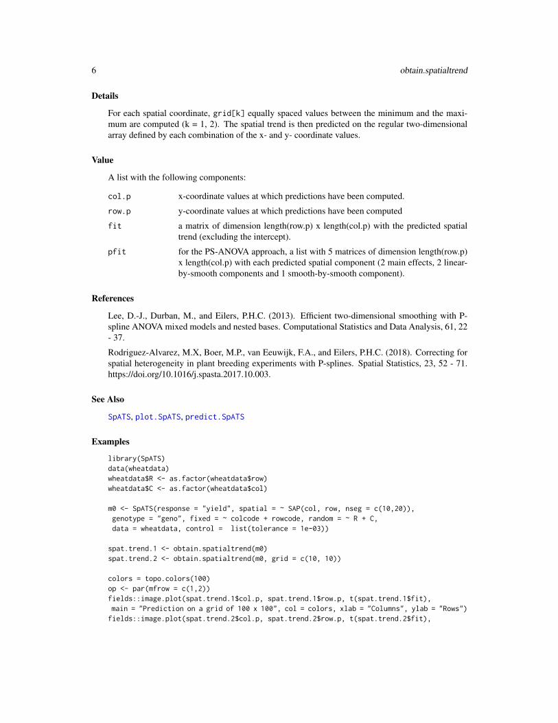
Details

For each spatial coordinate, grid[k] equally spaced values between the minimum and the maxi-mum are computed (k = 1, 2). The spatial trend is then predicted on the regular two-dimensionalarray defined by each combination of the x- and y- coordinate values.

Value

A list with the following components:

col.p x-coordinate values at which predictions have been computed.

row.p y-coordinate values at which predictions have been computed

fit a matrix of dimension length(row.p) x length(col.p) with the predicted spatialtrend (excluding the intercept).

pfit for the PS-ANOVA approach, a list with 5 matrices of dimension length(row.p)x length(col.p) with each predicted spatial component (2 main effects, 2 linear-by-smooth components and 1 smooth-by-smooth component).

References



See Also

SpATS, plot.SpATS, predict.SpATS

Examples


m0 <- SpATS(response = "yield", spatial = ~ SAP(col, row, nseg = c(10,20)),genotype = "geno", fixed = ~ colcode + rowcode, random = ~ R + C,data = wheatdata, control = list(tolerance = 1e-03))

spat.trend.1 <- obtain.spatialtrend(m0)spat.trend.2 <- obtain.spatialtrend(m0, grid = c(10, 10))

colors = topo.colors(100)op <- par(mfrow = c(1,2))fields::image.plot(spat.trend.1$col.p, spat.trend.1$row.p, t(spat.trend.1$fit),main = "Prediction on a grid of 100 x 100", col = colors, xlab = "Columns", ylab = "Rows")fields::image.plot(spat.trend.2$col.p, spat.trend.2$row.p, t(spat.trend.2$fit),

plot.SpATS 7

main = "Prediction on a grid of 10 x 10", col = colors, xlab = "Columns", ylab = "Rows")par(op)

plot.SpATS Default SpATS plotting

Description

Takes a fitted SpATS object produced by SpATS() and plots six different graphics (see Details).

Usage

## S3 method for class 'SpATS'plot(x, all.in.one = TRUE, main = NULL, annotated = FALSE, depict.missing = FALSE, ...)

Arguments

x an object of class SpATS as produced by SpATS().

all.in.one logical. If TRUE, the four plots are depicted in one window. Default is TRUE

main character string specifying the main title to appear on the plot. By default (i.e.when main = NULL), the variable under study is incorporated in the title of theplot.

annotated logical. If TRUE, the variable under study and the models used is added to theplot. Only applied when argument all.in.one is TRUE.

depict.missing logical. If TRUE, the estimated spatial trend is depicted for all plots in the field,even for those with missing values.


Details

The following graphics are depicted: the raw data, the fitted data (on the response scale), the (de-viance) residuals, the estimated spatial trend (excluding the intercept), the genotypic BLUEs (orBLUPs) and their histogram. Except for the histogram, the plots are depicted in terms of the spatialcoordinates (e.g., the rows and columns of the field).

References


See Also

SpATS

8 plot.variogram.SpATS

Examples


m0 <- SpATS(response = "yield", spatial = ~ SAP(col, row, nseg = c(10,20), degree = 3, pord = 2),genotype = "geno", fixed = ~ colcode + rowcode, random = ~ R + C, data = wheatdata,control = list(tolerance = 1e-03))

# Default plottingplot(m0)# Annotatedplot(m0, annotated = TRUE, main = "Wheat data (Gilmour et al., 1997)")

plot.variogram.SpATS Default variogram.SpATS plotting

Description

Takes a fitted variogram.SpATS object produced by variogram.SpATS() and plots the associatedsample variogram using an RGL 3D perspective plot (package plot3Drgl).

Usage

## S3 method for class 'variogram.SpATS'plot(x, min.length = 30, ...)

Arguments

x an object of class variogram.SpATS as produced by variogram.SpATS().

min.length numerical value. The sample variogram is depicted including only those pairswith more than min.length observations (see variogram.SpATS).


Details

This function as well as function variogram.SpATS() can only be used for regular two dimensionaldata.

References


Stefanova, K.T., Smith, A.B., and Cullis, B.R. (2009). Enhanced Diagnostics for the Spatial Anal-ysis of Field Trials. Journal of Agricultural, Biological, and Environmental Statistics, 14, 392 -410.

predict.SpATS 9

See Also

SpATS, variogram.SpATS

Examples



# Compute the variogramvar.m0 <- variogram(m0)# Plot the variogramplot(var.m0)

predict.SpATS Predictions from an SpATS object

Description

Takes a fitted SpATS object produced by SpATS() and produces predictions.

Usage

## S3 method for class 'SpATS'predict(object, newdata = NULL, which = NULL, ...)

Arguments

object an object of class SpATS as produced by SpATS().

newdata an optional data frame to be used for obtaining the predictions.

which an optional character string with the variables that define the margins of themultiway table to be predicted (see Details).


Details

This function allows to produce predictions, either specifying: (1) the data frame on which to obtainthe predictions (argument newdata), or (2) those variables that define the margins of the multiwaytable to be predicted (argument which). In the first case, all fixed components (including genotypewhen fixed) and the spatial coordinates must be present in the data frame. As for the randomeffects is concerned, they are excluded from the predictions when the value is missing in the dataframe. In the second case, predictions are obtained for each combination of values of the specified

10 print.SpATS

variables that is present in the data set used to fit the model. For those variables not specified in theargument which, the following rules have been considered: (a) random factors and the spatial trendare ignored in the predictions, (b) for fixed numeric variables, the mean value is considered; and (c)for fixed factors, the reference level is used.

Value

The data frame used for obtaining the predictions, jointly with the predicted values and the cor-responding standard errors. The label “Excluded” has been used to indicate those cases where acovariate has been excluded or ignored for the prediction (as for instance the random effect).

References

Welham, S., Cullis, B., Gogel, B., Gilmour, A., and Thompson, R. (2004). Prediction in linearmixed models. Australian and New Zealand Journal of Statistics, 46, 325 - 347.

See Also

SpATS, obtain.spatialtrend

Examples


m0 <- SpATS(response = "yield", spatial = ~ SAP(col, row, nseg = c(10,20)),genotype = "geno", fixed = ~ colcode + rowcode, random = ~ R + C,data = wheatdata, control = list(tolerance = 1e-03))

# Fitted values: prediction on the dataset used for fitting the modelpred1.m0 <- predict(m0, newdata = wheatdata)pred1.m0[1:5,]

# Genotype predictionpred2.m0 <- predict(m0, which = "geno")pred2.m0[1:5,]

print.SpATS Print method for SpATS objects

Description

Default print method for objects fitted with SpATS() function.

PSANOVA 11

Usage

## S3 method for class 'SpATS'print(x, ...)

Arguments

x an object of class SpATS as produced by SpATS()


Details

A short summary is printed including: the variable under study (response), the variable containingthe genotypes, the spatial model, and the random and fixed components (when appropriate). Besidesthis information, the number of observations used to fit the model, as well as of those deleted dueto missingness or zero weights are reported. Finally, the effective degrees of freedom (effectivedimension) of the fitted model and the (REML) deviance is also printed.

See Also

SpATS, summary.SpATS

Examples



m0

PSANOVA Define a two-dimensional penalised tensor-product of marginal B-Spline basis functions based on the P-spline ANOVA (PSANOVA) ap-proach.

Description

Auxiliary function used for modelling the spatial or environmental effect as a two-dimensionalpenalised tensor-product of marginal B-spline basis functions with anisotropic penalties on the basisof the PSANOVA approach by Lee et al. (2013).

Usage

PSANOVA(..., nseg = c(10,10), pord = c(2,2), degree = c(3,3), nest.div = c(1,1))

12 PSANOVA

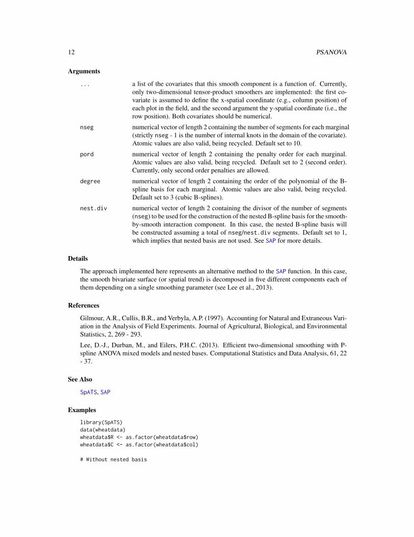
Arguments

... a list of the covariates that this smooth component is a function of. Currently,only two-dimensional tensor-product smoothers are implemented: the first co-variate is assumed to define the x-spatial coordinate (e.g., column position) ofeach plot in the field, and the second argument the y-spatial coordinate (i.e., therow position). Both covariates should be numerical.

nseg numerical vector of length 2 containing the number of segments for each marginal(strictly nseg - 1 is the number of internal knots in the domain of the covariate).Atomic values are also valid, being recycled. Default set to 10.

pord numerical vector of length 2 containing the penalty order for each marginal.Atomic values are also valid, being recycled. Default set to 2 (second order).Currently, only second order penalties are allowed.

degree numerical vector of length 2 containing the order of the polynomial of the B-spline basis for each marginal. Atomic values are also valid, being recycled.Default set to 3 (cubic B-splines).

nest.div numerical vector of length 2 containing the divisor of the number of segments(nseg) to be used for the construction of the nested B-spline basis for the smooth-by-smooth interaction component. In this case, the nested B-spline basis willbe constructed assuming a total of nseg/nest.div segments. Default set to 1,which implies that nested basis are not used. See SAP for more details.

Details

The approach implemented here represents an alternative method to the SAP function. In this case,the smooth bivariate surface (or spatial trend) is decomposed in five different components each ofthem depending on a single smoothing parameter (see Lee et al., 2013).

References



See Also

SpATS, SAP

Examples


# Without nested basis

SAP 13

m0 <- SpATS(response = "yield", spatial = ~ PSANOVA(col, row, nseg = c(10,20)),genotype = "geno", fixed = ~ colcode + rowcode, random = ~ R + C, data = wheatdata,control = list(tolerance = 1e-03))

summary(m0)

# With nested basism1 <- SpATS(response = "yield", spatial = ~ PSANOVA(col, row, nseg = c(10,20), nest.div = 2),genotype = "geno", fixed = ~ colcode + rowcode, random = ~ R + C, data = wheatdata,control = list(tolerance = 1e-03))

summary(m1)

SAP Define a two-dimensional penalised tensor-product of marginal B-Spline basis functions.

Description

Auxiliary function used for modelling the spatial or environmental effect as a two-dimensionalpenalised tensor-product of marginal B-spline basis functions with anisotropic penalties. The ap-proach implemented here corresponds to the Separation of Anisotropic Penalties (SAP) algorithmintroduced by Rodriguez-Alvarez et al. (2015).

Usage

SAP(..., nseg = c(10,10), pord = c(2,2), degree = c(3,3), nest.div = c(1,1),ANOVA = FALSE)

Arguments

... a list of the covariates that this smooth component is a function of. Currently,only two-dimensional tensor-product smoothers are implemented: the first co-variate is assumed to define the x-spatial coordinate (e.g., column position) ofeach plot in the field, and the second argument the y-spatial coordinate (i.e., therow position). Both covariates should be numerical.

nseg numerical vector of length 2 containing the number of segments for each marginal(strictly nseg - 1 is the number of internal knots in the domain of the covariate).Atomic values are also valid, being recycled. Default set to 10.

pord numerical vector of length 2 containing the penalty order for each marginal.Atomic values are also valid, being recycled. Default set to 2 (second order).

degree numerical vector of length 2 containing the order of the polynomial of the B-spline basis for each marginal. Atomic values are also valid, being recycled.Default set to 3 (cubic B-splines).

nest.div numerical vector of length 2 containing the divisor of the number of segments(nseg) to be used for the construction of the nested B-spline basis for the smooth-by-smooth interaction component. In this case, the nested B-spline basis will

14 SAP

be constructed assuming a total of nseg/nest.div segments. Default set to 1,which implies that nested basis are not used. See details.

ANOVA logical. If TRUE, four different smoothing parameters are considered: two forthe main effects and two for the smooth interaction. See details.

Details

Within the P-spline framework, anisotropic low-rank tensor-product smoothers have become thegeneral approach for modelling multidimensional surfaces (Eilers and Marx 2003; Wood 2006).In this package, we propose to model the spatial or environmental effect by means of the tensor-product of B-splines basis functions. In other words, we propose to model the spatial trend as asmooth bivariate surface jointly defined over the the spatial coordinates. Accordingly, the currentfunction has been designed to allow the user to specify the spatial coordinates that the spatial trend isa function of. There is no restriction about how the spatial coordinates shall be specified: these canbe the longitude and latitude of the position of the plot on the field or the column and row numbers.The only restriction is that the variables defining the spatial coordinates should be numeric (incontrast to factors).

As far as estimation is concerned, we have used in this package the equivalence between P-splinesand linear mixed models (Currie and Durban, 2002). Under this approach, the smoothing param-eters are expressed as the ratio between variance components. Moreover, the smooth componentsare decomposed in two parts: one which is not penalised (and treated as fixed) and one with ispenalised (and treated as random). For the two-dimensional case, the mixed model representationleads also to a very interesting decomposition of the penalised part of the bivariate surface in threedifferent components (Lee and Durban, 2011): (a) a component that contains the smooth maineffect (smooth trend) along one of the covariates that the surface is a function of (as, e.g, the x-spatial coordinate or column position of the plot in the field), (b) a component that contains thesmooth main effect (smooth trend) along the other covariate (i.e., the y-spatial coordinate or rowposition); and (c) a smooth interaction component (sum of the linear-by-smooth interaction compo-nents and the smooth-by-smooth interaction component). The default implementation used in thisfunction (ANOVA = FALSE) assumes two different smoothing parameters, i.e., one for each covari-ate in the smooth component. Accordingly, the same smoothing parameters are used for both, themain effects and the smooth interaction. However, this approach can be extended to deal with theANOVA-type decomposition presented in Lee and Durban (2011). In their approach, four differ-ent smoothing parameters are considered for the smooth surface, that are in concordance with theaforementioned decomposition: (a) two smoothing parameter, one for each of the main effects; and(b) two smoothing parameter for the smooth interaction component. Here, this decomposition canbe obtained by specifying the argument ANOVA = TRUE.

It should be noted that, the computational burden associated with the estimation of the two-dimensionaltensor-product smoother might be prohibitive if the dimension of the marginal bases is large. Inthese cases, Lee et al. (2013) propose to reduce the computational cost by using nested bases. Theidea is to reduce the dimension of the marginal bases (and therefore the associated number of pa-rameters to be estimated), but only for the smooth-by-smooth interaction component. As pointedout by the authors, this simplification can be justified by the fact that the main effects would infact explain most of the structure (or spatial trend) presented in the data, and so a less rich repre-sentation of the smooth-by-smooth interaction component could be needed. In order to ensure thatthe reduced bivariate surface is in fact nested to the model including only the main effects, Lee etal. (2013) show that the number of segments used for the nested basis should be a divisor of thenumber of segments used in the original basis (nseg argument). In the present function, the divisor

SAP 15

of the number of segments is specified through the argument nest.div. For a more detailed reviewon this topic, see Lee (2010) and Lee et al. (2013).

References

Currie, I., and Durban, M. (2002). Flexible smoothing with P-splines: a unified approach. StatisticalModelling, 4, 333 - 349.

Eilers, P.H.C., and Marx, B.D. (2003). Multivariate calibration with temperature interaction usingtwo-dimensional penalised signal regression. Chemometrics and Intelligent Laboratory Systems,66, 159 - 174.


Lee, D.-J., 2010. Smothing mixed model for spatial and spatio-temporal data. Ph.D. Thesis, De-partment of Statistics, Universidad Carlos III de Madrid, Spain.

Lee, D.-J., and Durban, M. (2011). P-spline ANOVA-type interaction models for spatio-temporalsmoothing. Statistical Modelling 11, 49 - 69.



Wood, S.N. (2006). Low-rank scale-invariant tensor product smooths for generalized additive mod-els. Journal of the Royal Statistical Society: Series B, 70, 495 - 518.

See Also

SpATS, PSANOVA

Examples


# Original anisotropic approach: two smoothing parametersm0 <- SpATS(response = "yield", spatial = ~ SAP(col, row, nseg = c(10,20)),genotype = "geno", fixed = ~ colcode + rowcode, random = ~ R + C,data = wheatdata, control = list(tolerance = 1e-03))

summary(m0)

# ANOVA decomposition: four smoothing parameters## Not run:m1 <- SpATS(response = "yield", spatial = ~ SAP(col, row, nseg = c(10,20), ANOVA = TRUE),genotype = "geno", fixed = ~ colcode + rowcode, random = ~ R + C, data = wheatdata,control = list(tolerance = 1e-03))

16 SpATS

summary(m1)

## End(Not run)

SpATS Spatial analysis of field trials with splines

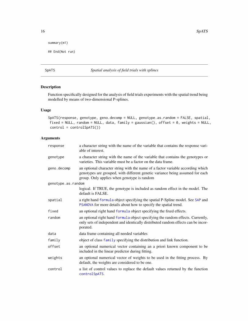
Description

Function specifically designed for the analysis of field trials experiments with the spatial trend beingmodelled by means of two-dimensional P-splines.

Usage

SpATS(response, genotype, geno.decomp = NULL, genotype.as.random = FALSE, spatial,fixed = NULL, random = NULL, data, family = gaussian(), offset = 0, weights = NULL,control = controlSpATS())

Arguments

response a character string with the name of the variable that contains the response vari-able of interest.

genotype a character string with the name of the variable that contains the genotypes orvarieties. This variable must be a factor on the data frame.

geno.decomp an optional character string with the name of a factor variable according whichgenotypes are grouped, with different genetic variance being assumed for eachgroup. Only applies when genotype is random

genotype.as.random

logical. If TRUE, the genotype is included as random effect in the model. Thedefault is FALSE.

spatial a right hand formula object specifying the spatial P-Spline model. See SAP andPSANOVA for more details about how to specify the spatial trend.

fixed an optional right hand formula object specifying the fixed effects.

random an optional right hand formula object specifying the random effects. Currently,only sets of independent and identically distributed random effects can be incor-porated.

data data frame containing all needed variables

family object of class family specifying the distribution and link function.

offset an optional numerical vector containing an a priori known component to beincluded in the linear predictor during fitting.

weights an optional numerical vector of weights to be used in the fitting process. Bydefault, the weights are considered to be one.

control a list of control values to replace the default values returned by the functioncontrolSpATS.

SpATS 17

Details

This function fits a (generalised) linear mixed model, with the variance components being estimatedby the restricted log-likelihood (REML). The estimation procedure is an extension of the SAP (Sep-aration of anisotropic penalties) algorithm by Rodriguez - Alvarez et al. (2015). In this package,besides the spatial trend, modelled as a two-dimensional P-spline, the implemented estimation al-gorithm also allows for the incorporation of both fixed and (sets of i.i.d) random effects on the(generalised) linear mixed model. As far as the implementation of the algorithm is concerned, thesparse structure of the design matrix associated with the genotype has been taken into account. Thecombination of both the SAP algorithm and this sparse structure makes the algorithm computationalefficient, allowing the proposal to be applied for the analysis of large datasets.

Value

A list with the following components:

call the matched call.

data the original supplied data argument with a new column with the weights usedduring the fitting process.

model a list with the model components: response, spatial, genotype, fixed and/or ran-dom.

fitted a numeric vector with the fitted values.

residuals a numeric vector with deviance residuals.

psi a two-length vector with the values of the dispersion parameter at convergence.For Gaussian responses both elements coincide, being the (REML) estimate ofdispersion parameter. For non-Gaussian responses, the result depends on the ar-gument update.psi of the controlSpATS function. If this argument was spec-ified to FALSE (the default), the first component of the vector corresponds to thedefault value used for the dispersion parameter (usually 1). The second element,correspond to the (REML) estimate of the dispersion parameter at convergence.If the argument update.psi was specified to TRUE, both components coincide(as in the Gaussian case).

var.comp a numeric vector with the (REML) variance component estimates. These vectorcontains the variance components associated with the spatial trend, as well asthose related with the random model terms.

eff.dim a numeric vector with the estimated effective dimension (or effective degrees offreedom) for each model component (genotype, spatial, fixed and/or random)

dim a numeric vector with the (model) dimension of each model component (geno-type, spatial, fixed and/or random). This value corresponds to the number ofparameters to be estimated

nobs number of observations used to fit the model

niterations number of iterations EM-algorithm

deviance the (REML) deviance at convergence (i.e., - 0.5 times the restricted log-likelihood)

coeff a numeric vector with the estimated fixed and random effect coefficients.

terms a list with the model terms: response, spatial, genotype, fixed and/or random.The information provided here is useful for printing and prediction purposes.

18 SpATS

vcov inverse of the coefficient matrix of the mixed models equations. The inverse isneeded for the computation of standard errors. For computational issues, theinverse is returned as a list: C11_inv corresponds to the coefficient matrix as-sociated with the genotype; C22_inv corresponds to the coefficient matrix asso-ciated with the spatial, the fixed and the random components; and C12_inv andC21_inv correspond to the “combination” of both.

References

Currie, I., and Durban, M. (2002). Flexible smoothing with P-splines: a unified approach. StatisticalModelling, 4, 333 - 349.

Eilers, P.H.C., and Marx, B.D. (2003). Multivariate calibration with temperature interaction usingtwo-dimensional penalised signal regression. Chemometrics and Intelligent Laboratory Systems,66, 159 - 174.

Eilers, P.H.C., Marx, B.D., Durban, M. (2015). Twenty years of P-splines. SORT, 39(2), 149 - 186.





See Also

SpATS-package, controlSpATS, SAP, PSANOVA

Examples

library(SpATS)data(wheatdata)summary(wheatdata)

# Create factor variable for row and columnswheatdata$R <- as.factor(wheatdata$row)wheatdata$C <- as.factor(wheatdata$col)


# Brief summarym0# More information: dimensions

summary.SpATS 19

summary(m0) # summary(fit.m2, which = "dimensions")# More information: variancessummary(m0, which = "variances")# More information: allsummary(m0, which = "all")

# Plot resultsplot(m0)plot(m0, all.in.one = FALSE)

# Variogramvar.m0 <- variogram(m0)plot(var.m0)

summary.SpATS Summary method for SpATS objects

Description

Default summary method for objects fitted with SpATS() function.

Usage

## S3 method for class 'SpATS'summary(object, which = c("dimensions", "variances", "all"), ...)

Arguments


which character vector indicating the information to be shown on the screen. “dimen-sions”: prints the dimensions associated to each component of the fitted model(see details), “variances”: prints the variance components and standard devi-ation (SD), the residual variance, and the ratio between the residual varianceand the variance components (in log10 scale); and, “all”: both dimensions andvariances are printed.


Details

This function provides relevant information about the fitted model. The dimensions associated toeach model term, as well as the variance components (jointly with the standard deviation), can beobtained. Specifically, the following information is shown:

dimensions dimensions associated to each model term (genotype, spatial, fixed and/or random):

• Effective: the effective dimension or effective degrees of freedom. The concept of effec-tive dimension is well known in the smoothing framework. However, its use has beenless recognized in the mixed model framework. The effective dimension of a fitted modelis defined as the trace of the so-called hat matrix (Hastie and Tibshirani, 1990). For each

20 summary.SpATS

model term, the effective dimension is then defined as the trace of the block of the hatmatrix corresponding to this term. For fixed effects, the effective dimension coincideswith the model dimension (see below). For random and smooth terms, however, the ef-fective dimension is usually lower than the model dimension. In these cases, the effectivedimension or effective degrees of freedom can be interpreted as the effective number ofestimated parameters. It is worth nothing that for the specification of the spatial trendusing the SAP function, the effective dimension associated to each spatial coordinates isshown (see Rodriguez-Alvarez et al. (2015) for details), as well as the global effectivedimension (the sum of these two values). For the ANOVA-type decomposition usingSAP, besides the former information, the effective dimension associated to each main ef-fect is also shown. This is in concordance with the number of smoothing parameters (orvariance components in the mixed model framework), used to model the spatial trend.Accordingly, for the spatial trend specified using the function PSANOVA, the effective di-mension of each of the five components is shown (and no global summary is reported).More information can be found in Rodriguez-Alvarez et al. (2018).

• Model: the model dimension corresponds to the number of parameters to be estimated.For the specification of the spatial trend using the SpATS function, the model and nominaldimensions are only specified for the global term (and for the main effects when usingthe ANOVA-type decomposition).

• Nominal: for the random terms of the model, the nominal dimension corresponds to themodel dimension minus one, “lost” due to the implicit constraint that ensures the meanof the random effects to be zero.

• Ratio: ratio between the nominal dimension and the model dimension. For the genotype(when random), this ratio corresponds to the generalized heritability proposed by Oakey(2006). A deeper discussion can be found in Rodriguez - Alvarez et al. (2018)

• Type: Model term type ’F’ Fixed, ’R’ Random, and ’S’ Smooth (spatial trend).

variances variance components associated to the random terms and the smooth spatial trend, aswell as the ratio between the residual variance and the variance components (in log10 scale).In the smoothing framework, this ratio corresponds to the smoothing parameter.

Value

Returns an object of class summary.SpATS with the same components as an SpATS object (seeSpATS) plus:

p.table.dim a matrix containing all the information related to the dimensions of the fittedmodel.

p.table.vc a matrix containing all the information related to the variance components of thefitted model

References

Hastie, T., and Tibshirani, R. (1990). Generalized Additive Models. In: Monographs on Statisticsand Applied Probability, Chapman and Hall, London.

Oakey, H., A. Verbyla, W. Pitchford, B. Cullis, and H. Kuchel (2006). Joint modeling of additiveand non-additive genetic line effects in single field trials. Theoretical and Applied Genetics, 113,809 - 819.

variogram 21



See Also

SpATS

Examples


# Create factor variable for row and columnswheatdata$R <- as.factor(wheatdata$row)wheatdata$C <- as.factor(wheatdata$col)


# Brief summarym0# More information: dimensionssummary(m0) # summary(fit.m2, which = "dimensions")# More information: variancessummary(m0, which = "variances")# More information: allsummary(m0, which = "all")

variogram Sample variogram

Description

Computes the sample variogram from an SpATS object.

Usage

## S3 method for class 'SpATS'variogram(x, ...)

Arguments

x an object of class SpATS as produced by SpATS().

... further arguments passed to or from other methods. Not yet implemented

22 variogram

Details

The present function computes the sample variogram on the basis of the (deviance) residuals of thefitted model. Currently, the function can only be applied for regular two-dimensional data, i.e, whenthe plots of the field are arranged in a regular two-dimensional array (usually defined by the columnand row positions). For each pair of (deviance) residuals ei and ej , the half-squared difference iscomputed

vij = 0.5(ei − ej)2,

as well as the corresponding column (cdij) and row displacements (rdij), with

cdij = |ci − cj |

andrdij = |ri − rj |,

where ck and rk denote the column and row position of plot k respectively. The sample variogramis then defined as the triplet

(cdij , rdij , v̄ij),

where v̄ij denotes the average of the vij that share the same column and row displacements. For amore detailed description, see Gilmour et al. (1997).

Value

An object of class variogram.SpATS with the following components:

data data frame including the following information: “value”: the value of the samplevariogram at each pair of column and row displacements; and “length”: the num-ber of observations used to compute the sample variogram at the correspondingpair of displacements.

col.displacement

numerical vector containing the column displacements

row.displacement

numerical vector containing the row displacements

References


Stefanova, K.T., Smith, A.B. and Cullis, B.R. (2009). Enhanced Diagnostics for the Spatial Analysisof Field Trials. Journal of Agricultural, Biological, and Environmental Statistics, 14, 392 - 410.

See Also

SpATS, plot.variogram.SpATS

wheatdata 23

Examples



# Compute the variogramvar.m0 <- variogram(m0)# Plot the variogramplot(var.m0)

wheatdata Wheat yield in South Australia

Description

A randomized complete block experiment of wheat in South Australia (Gilmour et al., 1997).

Usage

data("wheatdata")

Format

A data frame with 330 observations on the following 7 variables

yield yield, numeric

geno wheat variety, a factor with 107 levels

rep replicate factor, 3 levels

row row position, numeric

col column position, a numeric vector

rowcode a factor with 2 levels. This factor is related to the way the trial and the plots were sown(see Details).

colcode a factor with 3 levels. This factor is related to the way the plots were trimmed to anassumed equal length before harvest (see Details).

24 wheatdata

Details

A near complete block design experiment. In this experiment, a total of 107 varieties were sown in3 replicates in a near complete block design (3 varieties were sown twice in each replicate). Eachreplicate consisted of 5 columns and 22 rows. Accordingly, the field consists on 15 columns and22 rows (i.e. a total of 330 plots or observations). Trimming was done by spraying the wheat withherbicide. The sprayer travelled in a serpentine pattern up and down columns. More specifically,the plots were trimmed according to four possible combinations: up/down, down/down, down/up,and up/up. The colcode factor describe this 4-phase sequence. With respect to the way the trialwas sown, the procedure was done in a serpentine manner with a planter that seeded three rows ata time (Left, Middle, Right). This fact led to a systematic effect on the yield due to sowing. Thevariable rowcode describes the position of each plot in the triplet (Left, Middle, Right). Level 1was used for the middle plot, and 2 for those on the right or on the left of the triplet (see Gilmour etal. (1997) for more details).

Source


Kevin Wright (2015). agridat: Agricultural datasets. R package version 1.12. http://CRAN.R-project.org/package=agridat

Examples


Index

∗Topic datasetswheatdata, 23

∗Topic packageSpATS-package, 2

controlSpATS, 3, 16–18

family, 16formula, 16

getHeritability, 4

obtain.spatialtrend, 5, 10

plot.SpATS, 6, 7plot.variogram.SpATS, 8, 22predict.SpATS, 6, 9print.SpATS, 10PSANOVA, 11, 15, 16, 18, 20

SAP, 12, 13, 16, 18, 20SpATS, 4–7, 9–12, 15, 16, 20–22SpATS-package, 2summary.SpATS, 5, 11, 19

variogram, 21variogram.SpATS, 8, 9

wheatdata, 23

25

Package ‘SpATS’ - The Comprehensive R Archive Network · Package ‘SpATS’ March 6, 2018 Type...

Documents

Transcript of Package ‘SpATS’ - The Comprehensive R Archive Network · Package ‘SpATS’ March 6, 2018 Type...