Package ‘RAM’ · 6 assist.ado Arguments data an OTU table or a taxonomy abundance matrix....

Package ‘RAM’May 15, 2018

Type Package

Title R for Amplicon-Sequencing-Based Microbial-Ecology

Version 1.2.1.7

Date 2018-05-13

Author Wen Chen, Joshua Simpson, C. Andre Levesque

Maintainer Wen Chen <[email protected]>

Description Characterizing environmental microbiota diversity using amplicon-based next genera-tion sequencing (NGS) data. Functions are developed to manipulate operational taxo-nomic unit (OTU) table, perform descriptive and inferential statistics, and generate publication-quality plots.

License MIT + file LICENSE

Copyright Government of Canada

Depends vegan, ggplot2, stats

Imports RColorBrewer, gplots, plyr, reshape2, scales,labdsv, grid, gridExtra, ggmap, permute, VennDiagram, data.table, FD,MASS, RgoogleMaps, lattice, reshape, ade4, phangorn, phytools, utils,graphics, grDevices, ape

Suggests testthat, mapproj, gtable, indicspecies, Heatplus

Repository CRAN

URL https://cran.r-project.org/package=RAM, https://bitbucket.org/Wen_Chen/ram_releases/src/

BugReports https://bitbucket.org/Wen_Chen/ram_releases/issues/

NeedsCompilation no

R topics documented:RAM-package . . . . . . . . . . . . . . . . . . . . . . . . . . . . . . . . . . . . . . . . 3alignment . . . . . . . . . . . . . . . . . . . . . . . . . . . . . . . . . . . . . . . . . . 5assist.ado . . . . . . . . . . . . . . . . . . . . . . . . . . . . . . . . . . . . . . . . . . 5assist.NB . . . . . . . . . . . . . . . . . . . . . . . . . . . . . . . . . . . . . . . . . . 7

1

https://cran.r-project.org/package=RAM

https://bitbucket.org/Wen_Chen/ram_releases/src/

https://bitbucket.org/Wen_Chen/ram_releases/src/

https://bitbucket.org/Wen_Chen/ram_releases/issues/

2 R topics documented:

assist.ordination . . . . . . . . . . . . . . . . . . . . . . . . . . . . . . . . . . . . . . . 8col.splitup . . . . . . . . . . . . . . . . . . . . . . . . . . . . . . . . . . . . . . . . . . 9combine.OTU . . . . . . . . . . . . . . . . . . . . . . . . . . . . . . . . . . . . . . . . 10core.OTU . . . . . . . . . . . . . . . . . . . . . . . . . . . . . . . . . . . . . . . . . . 11core.OTU.rank . . . . . . . . . . . . . . . . . . . . . . . . . . . . . . . . . . . . . . . 12core.Taxa . . . . . . . . . . . . . . . . . . . . . . . . . . . . . . . . . . . . . . . . . . 14correlation . . . . . . . . . . . . . . . . . . . . . . . . . . . . . . . . . . . . . . . . . . 15data.clust . . . . . . . . . . . . . . . . . . . . . . . . . . . . . . . . . . . . . . . . . . 17data.revamp . . . . . . . . . . . . . . . . . . . . . . . . . . . . . . . . . . . . . . . . . 18data.subset . . . . . . . . . . . . . . . . . . . . . . . . . . . . . . . . . . . . . . . . . . 19dissim . . . . . . . . . . . . . . . . . . . . . . . . . . . . . . . . . . . . . . . . . . . . 20dissim.heatmap . . . . . . . . . . . . . . . . . . . . . . . . . . . . . . . . . . . . . . . 22dissim.plot . . . . . . . . . . . . . . . . . . . . . . . . . . . . . . . . . . . . . . . . . . 24diversity.indices . . . . . . . . . . . . . . . . . . . . . . . . . . . . . . . . . . . . . . . 26envis.NB . . . . . . . . . . . . . . . . . . . . . . . . . . . . . . . . . . . . . . . . . . 28factor.abundance . . . . . . . . . . . . . . . . . . . . . . . . . . . . . . . . . . . . . . 29filter.META . . . . . . . . . . . . . . . . . . . . . . . . . . . . . . . . . . . . . . . . . 30filter.OTU . . . . . . . . . . . . . . . . . . . . . . . . . . . . . . . . . . . . . . . . . . 31filter.Taxa . . . . . . . . . . . . . . . . . . . . . . . . . . . . . . . . . . . . . . . . . . 32fread.meta . . . . . . . . . . . . . . . . . . . . . . . . . . . . . . . . . . . . . . . . . . 33fread.OTU . . . . . . . . . . . . . . . . . . . . . . . . . . . . . . . . . . . . . . . . . . 34get.rank . . . . . . . . . . . . . . . . . . . . . . . . . . . . . . . . . . . . . . . . . . . 35group.abund.Taxa . . . . . . . . . . . . . . . . . . . . . . . . . . . . . . . . . . . . . . 36group.abundance . . . . . . . . . . . . . . . . . . . . . . . . . . . . . . . . . . . . . . 37group.abundance.meta . . . . . . . . . . . . . . . . . . . . . . . . . . . . . . . . . . . 39group.diversity . . . . . . . . . . . . . . . . . . . . . . . . . . . . . . . . . . . . . . . 40group.heatmap . . . . . . . . . . . . . . . . . . . . . . . . . . . . . . . . . . . . . . . 42group.heatmap.simple . . . . . . . . . . . . . . . . . . . . . . . . . . . . . . . . . . . . 44group.indicators . . . . . . . . . . . . . . . . . . . . . . . . . . . . . . . . . . . . . . . 45group.OTU . . . . . . . . . . . . . . . . . . . . . . . . . . . . . . . . . . . . . . . . . 47group.rich . . . . . . . . . . . . . . . . . . . . . . . . . . . . . . . . . . . . . . . . . . 49group.spatial . . . . . . . . . . . . . . . . . . . . . . . . . . . . . . . . . . . . . . . . . 50group.spec . . . . . . . . . . . . . . . . . . . . . . . . . . . . . . . . . . . . . . . . . . 51group.Taxa.bar . . . . . . . . . . . . . . . . . . . . . . . . . . . . . . . . . . . . . . . 52group.Taxa.box . . . . . . . . . . . . . . . . . . . . . . . . . . . . . . . . . . . . . . . 54group.temporal . . . . . . . . . . . . . . . . . . . . . . . . . . . . . . . . . . . . . . . 55group.venn . . . . . . . . . . . . . . . . . . . . . . . . . . . . . . . . . . . . . . . . . 56ITS1/ITS2 . . . . . . . . . . . . . . . . . . . . . . . . . . . . . . . . . . . . . . . . . . 58LCA.OTU . . . . . . . . . . . . . . . . . . . . . . . . . . . . . . . . . . . . . . . . . . 59location.formatting . . . . . . . . . . . . . . . . . . . . . . . . . . . . . . . . . . . . . 60match.data . . . . . . . . . . . . . . . . . . . . . . . . . . . . . . . . . . . . . . . . . . 61meta . . . . . . . . . . . . . . . . . . . . . . . . . . . . . . . . . . . . . . . . . . . . . 62META.clust . . . . . . . . . . . . . . . . . . . . . . . . . . . . . . . . . . . . . . . . . 63network_data . . . . . . . . . . . . . . . . . . . . . . . . . . . . . . . . . . . . . . . . 64OTU.diversity . . . . . . . . . . . . . . . . . . . . . . . . . . . . . . . . . . . . . . . . 65OTU.ord . . . . . . . . . . . . . . . . . . . . . . . . . . . . . . . . . . . . . . . . . . . 66OTU.rarefy . . . . . . . . . . . . . . . . . . . . . . . . . . . . . . . . . . . . . . . . . 68OTU.recap . . . . . . . . . . . . . . . . . . . . . . . . . . . . . . . . . . . . . . . . . . 69

RAM-package 3

pcoa.plot . . . . . . . . . . . . . . . . . . . . . . . . . . . . . . . . . . . . . . . . . . . 71percent.classified . . . . . . . . . . . . . . . . . . . . . . . . . . . . . . . . . . . . . . 73phylog_taxonomy . . . . . . . . . . . . . . . . . . . . . . . . . . . . . . . . . . . . . . 74phylo_taxonomy . . . . . . . . . . . . . . . . . . . . . . . . . . . . . . . . . . . . . . 75RAM.dates . . . . . . . . . . . . . . . . . . . . . . . . . . . . . . . . . . . . . . . . . 77RAM.factors . . . . . . . . . . . . . . . . . . . . . . . . . . . . . . . . . . . . . . . . 77RAM.input.formatting . . . . . . . . . . . . . . . . . . . . . . . . . . . . . . . . . . . 78RAM.pal . . . . . . . . . . . . . . . . . . . . . . . . . . . . . . . . . . . . . . . . . . 79RAM.plotting . . . . . . . . . . . . . . . . . . . . . . . . . . . . . . . . . . . . . . . . 79RAM.rank.formatting . . . . . . . . . . . . . . . . . . . . . . . . . . . . . . . . . . . . 81read.meta . . . . . . . . . . . . . . . . . . . . . . . . . . . . . . . . . . . . . . . . . . 81read.OTU . . . . . . . . . . . . . . . . . . . . . . . . . . . . . . . . . . . . . . . . . . 82reset.META . . . . . . . . . . . . . . . . . . . . . . . . . . . . . . . . . . . . . . . . . 83sample.locations . . . . . . . . . . . . . . . . . . . . . . . . . . . . . . . . . . . . . . . 84sample.map . . . . . . . . . . . . . . . . . . . . . . . . . . . . . . . . . . . . . . . . . 85sample.sites . . . . . . . . . . . . . . . . . . . . . . . . . . . . . . . . . . . . . . . . . 87seq_var . . . . . . . . . . . . . . . . . . . . . . . . . . . . . . . . . . . . . . . . . . . 88shared.OTU . . . . . . . . . . . . . . . . . . . . . . . . . . . . . . . . . . . . . . . . . 90shared.Taxa . . . . . . . . . . . . . . . . . . . . . . . . . . . . . . . . . . . . . . . . . 91tax.abund . . . . . . . . . . . . . . . . . . . . . . . . . . . . . . . . . . . . . . . . . . 92tax.fill . . . . . . . . . . . . . . . . . . . . . . . . . . . . . . . . . . . . . . . . . . . . 93tax.split . . . . . . . . . . . . . . . . . . . . . . . . . . . . . . . . . . . . . . . . . . . 95Taxa.ord . . . . . . . . . . . . . . . . . . . . . . . . . . . . . . . . . . . . . . . . . . . 96theme_ggplot . . . . . . . . . . . . . . . . . . . . . . . . . . . . . . . . . . . . . . . . 98top.groups.plot . . . . . . . . . . . . . . . . . . . . . . . . . . . . . . . . . . . . . . . 99transpose.LCA . . . . . . . . . . . . . . . . . . . . . . . . . . . . . . . . . . . . . . . 100transpose.OTU . . . . . . . . . . . . . . . . . . . . . . . . . . . . . . . . . . . . . . . 101valid.OTU . . . . . . . . . . . . . . . . . . . . . . . . . . . . . . . . . . . . . . . . . . 102valid.taxonomy . . . . . . . . . . . . . . . . . . . . . . . . . . . . . . . . . . . . . . . 102write.data . . . . . . . . . . . . . . . . . . . . . . . . . . . . . . . . . . . . . . . . . . 103

Index 105

RAM-package Analysis of Amplicon-Based Metagenomic Data

Description

The RAM package provides a series of functions to make amplicon based metagenomic analysismore accessible. The package is designed especially for those who have little or no experience withR. This package calls heavily upon other packages (such as vegan and ggplot2), but the functionsin this package either extend their functionality, or increase the ease-of-use.

4 RAM-package

Details

Package: RAMType: PackageVersion: 1.2.0Date: 2014-12-10License: MIT License, Copyright (c) 2014 Government of Canada

Load data from .csv-formatted OTU files with read.OTU or fread.OTU, then process the data withother commands. Type the command library(help = RAM) for a full index of all help topics, orls("package:RAM") to get a list of all functions in the package. Type data(ITS1, ITS2, meta)to load sample data sets of RAM, which include the following data of 16 samples: 1) ITS1: OTUtable of fungal internal transcribed spacer region1 3) ITS2: OTU table of fungal internal transcribedspacer region2 3) meta: associated metadata 4) alignment for seq_var Type citation("RAM") forhow to cite this package. This pacakge contains information licensed under the Open GovernmentLicence - Canada. See group.spatial for further details.

Author(s)

Wen Chen and Joshua Simpson. Maintainer: Wen Chen <[email protected]>

See Also

vegdist, ggplot

Examples

## Not run:# load data from your own files...otu1 <- fread.OTU("path/to/OTU/table")otu2 <- read.OTU("path/to/OTU/table")meta1 <- fread.meta("path/to/meta/table")meta2 <- read.meta("path/to/meta/table")# ...or use the included sample datadata(ITS1, ITS2, meta)data <- list(ITS1=ITS1, ITS2=ITS2)dissim.heatmap(ITS1, meta, row.factor=c(City="City"))dissim.alleig.plot(data)data(alignment)# type library(help = RAM) to get a full listing of helpdocuments

## End(Not run)

alignment 5

alignment Sample Alignment

Description

This is an alignment for seq_var package.

Usage

data(alignment)

Format

An alignment with sequence ID being formatted as follows: genus_name:accession:genus:species:strain_info/seqBegin-seqEnd. The location of each party can be rearranged, and the separator can be other speciall char-acters, such as "|".

Source

Wen Chen

Examples

data(alignment)str(alignment)alignment

assist.ado Perform ADONIS Analysis for OTU Tables Or Taxonomic AbundanceMatrix

Description

This function simplifies ADONIS analysis by abstracting away some of the complexity and return-ing a list of useful measures.

Usage

assist.ado(data, meta, is.OTU=TRUE, ranks=NULL,data.trans=NULL, dist=NULL, meta.strata=NULL,perm=1000, top=NULL, mode="number")

6 assist.ado

Arguments

data an OTU table or a taxonomy abundance matrix.

is.OTU logical. If the data is an OTU table, set is.OTU TRUE; otherwise, set it as FALSE.

meta the metadata table to be used (must have same samples as data.

ranks optional. If ranks is not provided, will test for OTUs, otherwise, will test ontaxa at defined ranks. If data is a taxonomic abundance matrix, ranks can beNULL

data.trans optional. Transform the data using method from the function decostand

dist optional. the name of any method used in vegdist to calculate pairwise dis-tances. See also adonis and vegdist.

meta.strata optional. A metadata variable within which to constrain permutations. See alsoadonis

perm a numeric number of replicate permutations used for the hypothesis test used inadonis.

top optional. Select the top taxa or OTUs. See also data.revamp

mode a character vector, one of "percent" or "number". If number, then top groupswill be selected based on total sequence count. If percent, then top groups willbe selected based on relative abundance. See also data.revamp

Value

This function returns a list containing outputs from adonis test.

• If is.OTU is TRUE and ranks is not given: the output is a length one list named LCA_OTU.

• If is.OTU is TRUE and ranks is given: the output is a list with a length same as the number oftaxonomic ranks provided. Each member of the list is named after the rank it processed at.

• If is.OTU is FALSE, the output is a length one list named Taxa.

Author(s)

Wen Chen.

See Also

adonis

Examples

data(ITS1, meta)## Not run:# test OTUsdata <- list(ITS1=ITS1, ITS2=ITS2)assist.ado(data=data, is.OTU=TRUE,meta=meta, ranks=NULL,

data.trans="log", dist=NULL)# test taxa at different ranksranks <- c("p", "c", "o", "f", "g")

assist.NB 7

ado <- assist.ado(data=data, is.OTU=TRUE,meta=meta, ranks=ranks,data.trans="log", dist="bray" )

# test generag1 <- tax.abund(otu1=ITS1, rank="g", drop.unclassified=TRUE)data <- list(g1=g1)assist.ado(data=data, is.OTU=FALSE,

meta=meta, ranks=NULL,data.trans="log", dist="bray" )

## End(Not run)

assist.NB Negative Binomial Test For OTUID or Taxon

Description

This function does negative binomial test for a given otuID or taxon

Usage

assist.NB(data, meta, is.OTU=TRUE, rank=NULL, meta.factors=NULL,anov.fac=NULL, taxon="")

Arguments

data an ecology data set to be analyzed.

meta the metadata table to be analyzed.

is.OTU logical. If an OTU table was provided, is.OTU should be set as TRUE; otherwise,it should be set as FALSE.

rank optional. If no rank was provided, the data will be used as it is, if rank isprovided, if data is an OTU table, it will be converted to taxonomic abundancematrix at the given rank, no change will be made for a data that has already beena taxonomic abundance matrix. See also tax.abund and data.revamp

meta.factors optional. If provided, will only test the model on selected metadata variables;otherwise, will test all variables in the metadata table.

anov.fac optional. Whether or not to do anova test on a metadata variable.

taxon a length one charactor. Can either be an otuID or a taxon name.

Value

This function return a list of outputs of the negative bionomial modeling for a selected otuID ortaxa. Members of this output list are: "NB.model", "tax.met", "taxon", "factors", "anova".

NB.model is the negative bionomial model

tax.met is a dataframe with combined the taxon and metadata

8 assist.ordination

taxon is either a taxon name or in LCA_otuID format, see also LCA.OTU

factors shows which metadata variable had significant impact

anova shows anova test of a metadata variable, this will not be available if anov.facis NULL

Author(s)

Wen Chen

Examples

data(ITS1, meta)m <- meta[, c(2,3,5,7)]## Not run:# for usage demonstration purpose only, may not fit the negative# binomial distribution model.nb <- assist.NB(ITS1, meta=m, rank="g",

anov.fac="Harvestmethod",taxon=rownames(ITS1)[1])

## End(Not run)

assist.ordination Perform CCA and RDA Analysis for OTU Tables

Description

This function simplifies CCA and RDA analysis by abstracting away some of the complexity andreturning a list of useful measures.

Usage

assist.cca(otu1, otu2 = NULL, meta, full = TRUE, exclude = NULL,rank, na.action=na.exclude)

assist.rda(otu1, otu2 = NULL, meta, full = TRUE, exclude = NULL,rank, na.action=na.exclude)

Arguments

otu1 the first OTU table to be used.

otu2 the second OTU table to be used.

meta the metadata table to be used (must have same samples as otu1/otu2).

full logical. Should a full model be considered? (If not, a restricted model is used).

exclude A vector, either numeric or logical, specifying the columns to be removed frommeta. If a character vector, columns with those names will be removed; if anumeric vector, columns with those indices will be removed.

col.splitup 9

rank a character vector representing a rank. Must be in one of three specific formats(see ?RAM.rank.formatting for help).

na.action choice of one of the following: "na.fail", "na.omit" or "na.exclude", see na.actionin cca for detail.

Value

If both otu1 and otu2 are given, a list of length 2 will be returned with the following items (if onlyotu1 is given, a list of length 1 will be returned with these items):

$GOF the goodness of fit scores for the model.

$VIF the VIF scores for the model.$percent_variation

the percent variation explained by each axis

$CCA_eig Eigenvalues for CCA axes.

$CA_eig Eigenvalues for CA axes.

$anova the ANOVA results for the model.

Author(s)

Wen Chen and Joshua Simpson.

See Also

cca, anova.cca

Examples

data(ITS1, meta)cca.help <- assist.cca(ITS1, meta=meta, rank="p")cca.help$anova

col.splitup Split Column Of Data Frame

Description

This function output consumes a data frame and split one by defined separator.

Usage

col.splitup(df, col="", sep="", max=NULL, names=NULL, drop=TRUE)

10 combine.OTU

Arguments

df a data frame.col name of a column in df.sep the separator to split the column. It can be regular expression.max optional. The number of columns to be split to.names optional. The names for the new columns.drop logical. Whether or not to keep the original column to be split in the output.

Value

The value returned by this function is a data frame. The selected column is split each separator andappended to the original data frame. The original column may may not to be kept in the output asdefined by option drop.

The number of columns to be split to depends on three factors, 1) the maximum columns that theoriginal column can be split to by each separator; 2) the user definde max; and 3) the length of thecolumn names defined by names. This function will split the column to the maximun number of the3, empty columns will be filled with empty strings.

Author(s)

Wen Chen.

Examples

data(ITS1)# filter.OTU() returns a listotu <- filter.OTU(list(ITS1=ITS1), percent=0.001)[[1]]# split and keep taxonomy columnotu.split <- col.splitup(otu, col="taxonomy", sep="; ",

drop=FALSE)## Not run:# give new column namestax.classes <- c("kingdom", "phylum", "class",

"order", "family", "genus")otu.split <- col.splitup(otu, col="taxonomy", sep="; ",

drop=TRUE, names=tax.classes)

## End(Not run)

combine.OTU Combine Non Overlapped OTU tables From The Same Community

Description

This function combines otu tables from the same community but based on independent sequencingruns. Such combined otu table gives a more complete profile of the microbial community than eachindividual otu table does. This function should NOT be used to combine ITS1 and ITS2 otu tablesif they were extracted from long NGS sequences.

core.OTU 11

Usage

combine.OTU(data, meta)

Arguments

data a list of otu tables to be combined.

meta the metadata that should have the same number and order of the samples as theotu tables do.

Value

combine.OTU returns a data frame of combined otu tables which have the same samples. Samplesin the output will match those in the metadata provided.

Author(s)

Wen Chen

See Also

match.data

Examples

data(ITS1, ITS2, meta)meta.new <- head(meta)## Not run:# for demonstration purposes only, Not recommend to combine# ITS1 and ITS2 otu tables that both regions were extracted from# long NGS sequencescomb <- combine.OTU(data=list(ITS1=ITS1, ITS2=ITS2), meta=meta.new)stopifnot(identical(colnames(comb)[1:(ncol(comb)-1)],

rownames(meta.new)))

## End(Not run)

core.OTU Summary Of Core OTUs

Description

This function returns a list showing otus that present in a pre-defined percent of samples in eachlevel of a given metadata category.

Usage

core.OTU(data, meta, meta.factor="", percent=1)

12 core.OTU.rank

Arguments

data a list of OTU tables to be analyzed. See RAM.input.formatting.


meta.factor the metadata qualitative variable

percent the percent of samples in each level of the given metadata variable

Value

core.OTU returns a list containing otus that present in a pre-defined percent of samples in each levelof a given metadata category. The outputs describe the following information for each level of agiven metadata variable: 1) core otuID; 2) taxa the core otus assigned to; and 3) percent of core otussequences vs. total sequences in each levels of the given metadata variable. The last item in the listshow the same information of otus that in all levels.

Note

The OTUs are determined to be absent/present using the "pa" method from the function decostand.

Author(s)

Wen Chen

See Also

decostand

Examples

data(ITS1, meta)## Not run:data <- list(ITS1=ITS1)core <- core.OTU(data=data, meta=meta,

meta.factor="City", percent=0.90)

## End(Not run)

core.OTU.rank Summary Of Core OTUs

Description

This function returns a list showing otus that present in a pre-defined percent of samples in eachlevel of a given metadata category.

Usage

core.OTU.rank(data, rank="g", drop.unclassified=TRUE,meta, meta.factor="", percent=1)

core.OTU.rank 13

Arguments

data a list of OTU tables to be analyzed. See also RAM.input.formatting.

rank the taxonomic rank(s) of otu classification (see ?RAM.rank.formatting for for-matting details).

drop.unclassified

logical, whether or not exclude unclassified groups.




Value

core.OTU.rank returns a list containing otus that present in a pre-defined percent of samples ineach level of a given metadata category. The outputs describe the following information for eachlevel of a given metadata variable: 1) core otuID; 2) taxa the core otus assigned to; and 3) percentof core otus sequences vs. total sequences in each group. The last item in the list show the sameinformation of otus that in all levels.

Note

The taxon groups are determined to be absent/present using the "pa" method from the functiondecostand.

Author(s)

Wen Chen

See Also

decostand

Examples

data(ITS1, meta)## Not run:core <- core.OTU.rank(data=list(ITS1=ITS1), rank="g", meta=meta,

meta.factor="City", percent=0.90)

## End(Not run)

14 core.Taxa

core.Taxa Show Summary of Core Taxa

Description

This function returns a list showing taxa at the given taxonomic rank that present in a pre-definedpercent of samples in each level of a given metadata category.

Usage

core.Taxa(data, is.OTU=FALSE, rank="g",drop.unclassified=TRUE,meta, meta.factor="", percent=1)

Arguments

data a list of OTU tables or taxonomy abundance matrices.

is.OTU logical. If TRUE, data is an OTU table; otherwise a taxonomy abundance matrixshould be provided.

rank the taxonomic rank of classification (see ?RAM.rank.formatting for formattingdetails).

drop.unclassified

logical, whether or not exclude unclassified groups. See also tax.abund




Value

core.Taxa returns a list containing taxa at a given rank that present in a pre-defined percent ofsamples in each level of a given metadata category. The outputs describe the following informationfor each level of a given metadata variable: 1) core taxa; 2) percent of core taxa sequences vs. totalsequences in each levels of the given metadata variable. The last item in the list show the sameinformation of taxa that in all levels.

Note

The taxa are determined to be absent/present using the "pa" method from the function decostand.

Author(s)

Wen Chen

See Also

decostand

correlation 15

Examples

data(ITS1, meta)# taxa shared by 50 percent samples of each citycore <- core.Taxa(data=list(ITS1=ITS1), is.OTU=TRUE, meta=meta,

rank="g", meta.factor="City", percent=0.5)## Not run:data(ITS1, ITS2, meta)core <- core.Taxa(data=list(ITS1=ITS1, ITS2=ITS2), is.OTU=TRUE,

meta=meta, rank="g", meta.factor="City",percent=0.7)

# use taxonomy abundance matrixg1<-tax.abund(ITS1, rank="g")core <- core.Taxa(data=list(genus_ITS1=g1), is.OTU=FALSE,

meta=meta, rank="g", meta.factor="City",percent=0.9)

## End(Not run)

correlation Plot Of Correlation Coefficient

Description

This function plot correlation relationship among taxa at a give rank and / or numeric variables ofmetadata.

Usage

correlation(data=NULL, is.OTU=TRUE, meta=NULL, rank="g",sel=NULL, sel.OTU=TRUE, data.trans=NULL,method="pearson", main=NULL, file=NULL,ext=NULL, width=8, height=8)

Arguments

data a data frame that either an OTU table or taxonomy abundance matrix, can bemissing but if metadata is also missing, an error message will be raised.

is.OTU logical. Whether or not the data is an OTU table.

meta the metadata table to be used.

rank the taxonomic rank to use (see ?RAM.rank.formatting for formatting details).

sel optional. It is a character vector of selected otuIDs or taxa names at a giventaxonomic rank. If provided, sel.OTU should be set to decribe the type of IDs,i.e. TRUE means otuIDs, FALSE means taxa names. If provide, only the selectedtaxa will be ploted; otherwise, all taxa will be ploted.

sel.OTU logical. Whether or not the selected items from data are otuIDs. If FALSE, selshould be a string vector of taxa names at a given rank.

16 correlation

data.trans a character string of one of the following, "total", "log", "hellinger" etc, see?vegan::decostand for details and other data transformation methods.

method a character string, can be one of the following, "pearson", "kendall", "spearman"for the calculation of correlation coefficient (or covariance) is to be computed(see ?stats::cor for details)

main a character string. The title of the plot.

file the file path where the image should be created (see ?RAM.plotting).

ext filename extension, the type of image to be saved to. (see ?RAM.plotting).

height the height of the image to be created (in inches).

width the width of the image to be created (in inches).

Details

This function uses stats::cor to calculate correlation coefficient (or covariance), and uses lattice::levelplotto generate the graph. (see References) Option sel is optional, however, it raises an error if the totalnumber of variables to be plotted was too big, and no plot will be generated.

Value

This function generates a graph showing correlation relationship among OTUs or taxa at a givenrank, and numeric variables of metadata

Author(s)

Wen Chen.

References

Sarkar, Deepayan (2008) _Lattice: Multivariate Data Visualization with R_, Springer. <URL:http://lmdvr.r-forge.r-project.org/>

Becker, R. A., Chambers, J. M. and Wilks, A. R. (1988) _The New S Language_. Wadsworth &Brooks/Cole.

See Also

cor levelplot

Examples

data(ITS1, meta)# only plot the first 10 OTUssel <- rownames(ITS1)[1:10]correlation(data=ITS1, meta=meta, is.OTU=TRUE, sel.OTU=TRUE,

sel=sel)## Not run:sel <- c("Fusarium", "Cladosporium", "Alternaria")correlation(data=ITS1, meta=meta, is.OTU=TRUE, sel.OTU=FALSE,

sel=sel, rank="g", data.trans="total",

data.clust 17

file="test.pdf", ext="pdf")

## End(Not run)

data.clust Plot Hierarchical Cluster Of Samples Based on OTU Table or Taxo-nomic Abundance Matrix

Description

This function plot hierarchical cluster Of ecology data set.

Usage

data.clust(data, is.OTU=TRUE, meta, rank=NULL, top=NULL,mode="number", group=4, data.trans=NULL,dist=NULL, clust=NULL, type=NULL, main=NULL,file=NULL, ext=NULL, width=8, height=8)

Arguments

data an ecology data set to be analyzed.


meta the metadata table associated with ecology data set.


top the top otuIDs or taxa to be considered for the clustering analysis. See alsodata.revamp

mode either be "number" or "percent". See also data.revamp

group an integer or a metadata variable. If an integar, will cut tree into correspondinggroups and color them accordingly; if a metadata variable was provided, treeleaves (sampleIDs) will be colored by each level.

data.trans optional. If was provided, numeric data will be transformed. See also decostand

dist optional. If was provided, distance matrix will be calculated using the givenmethod; otherwise use vegdist default Bray-Curtis method. See also vegdistand gowdis.

clust optional. If was not provided, will use the default agglomeration method used byhclust, i.e. "complete". Otherwise, will used user defined method for clustering.See also hclust.

type optional. Can be one of the following: "triangle", "rectangle", "phylogram","cladogram", "fan", "unrooted", "radial".

18 data.revamp

main The title of the plot.

file optional. Filename that the plot to be saved to.

ext optional. File type that the plot to be saved to.

width an integer, width of the plot.

height an integer, height of the plot.

Value

This function returns a tree plot of the hierarchical cluster of the samples based on ecological data.

Author(s)

Wen Chen

Examples

data(ITS1, meta)## Not run:data.clust(data=ITS1, is.OTU=TRUE, data.trans="total",

dist="bray", type="fan", meta=meta, group="Plots")

## End(Not run)

data.revamp Transform OTU Table

Description

This function consumes and transforms either an OTU table or a taxonomy abundance matrix. Ifan OTU table was provided, it will be either transposed without the "taxonomy" column, but eachotuID will be renames with it’s LCA classification appended; or being transformed to be taxonomicabundance matrix at the ranks set by ranks. If a taxonomic abundance matrix is provided, it willbe kept the same with proper data transformation as defined by stand.method option.

Usage

data.revamp(data, is.OTU=TRUE, ranks=NULL, stand.method=NULL,top=NULL, mode="number")

Arguments

data an OTU table or a taxonomic abundance matrix.


data.subset 19

ranks optional. If no ranks was provided, the OTU table will be processed by LCA.OTUand then transposed with sampleIDs being row names and otuIDs being columnnames. If ranks was provided, the OTU table will be processed by tax.abund ateach given taxonomic ranks. See also RAM.rank.formatting. The unclassifiedtaxon groups are removed.

stand.method optional. Transform the output using method from the function decostand

top optional. Select the top taxa or OTUs.

mode a character vector, one of "percent" or "number". If number, then top manygroups will be selected. If percent, then all groups with relative abundance inat least one sample above top will be selected.

Value

The value returned by this function is a list, so for convenience, any nested lists have been givendescriptive items names to make accessing its elements simple (see Examples).

• If is.OTU is TRUE and ranks is not given: the output is a length one list named LCA_OTU.

• If is.OTU is TRUE and ranks is given: the output is a list with a length same as the number oftaxonomic ranks provided. Each member of the list is named after the rank it processed at.

• If is.OTU is FALSE, the output is a length one list named Taxa.

Author(s)

Wen Chen

Examples

data(ITS1, ITS2, meta)data.new <- data.revamp(data=list(ITS1=ITS1), is.OTU=TRUE,

ranks=c("f", "g"), stand.method="log")## Not run:data.new <- data.revamp(data=list(ITS1=ITS1), is.OTU=TRUE,

ranks=NULL, stand.method="log")data.new <- data.revamp(data=list(ITS1=ITS1, ITS2=ITS2),

is.OTU=TRUE, ranks=c("f", "g"), stand.method="total")names(data.new)

## End(Not run)

data.subset Subset OTU And Metadata

Description

This function subset OTUs and metadata based on user defined values of metadata variables.

20 dissim

Usage

data.subset(data, meta, factors="", values="", and=TRUE)

Arguments

data a list of otu tables to be processed. See also RAM.input.formatting.

meta the metadata for subset.

factors a vector containing metadata variables.

values a vector containing values of interest in metadata variables.

and logical. Determine whether all conditions needs to be met or not.

Value

The value returned by this function is a list containing otu tables matching the filtering requirement.The last item in the output list is the associated new metadata table fit the requirement.

Author(s)

Wen Chen

Examples

data(ITS1, ITS2, meta)names(meta)factors <- c("City", "Harvestmethod")values <- c("City1", "Method1")# match all requirements, and=TRUEsub <- data.subset(data=list(ITS1=ITS1, ITS2=ITS2), meta=meta,

factors=factors, values=values, and=TRUE)# match either of the requirements, and=FALSEsub <- data.subset(data=list(ITS1=ITS1, ITS2=ITS2), meta=meta,

factors=factors, values=values, and=FALSE)## Not run:names(sub)ITS1.sub <- sub[["ITS1"]]ITS2.sub <- sub[["ITS2"]]meta.sub <- sub[["meta"]]

## End(Not run)

dissim Calculate Dissimilarity Matrix Data

Description

These functions calculate different measures related to dissimilarity matrices. All of these functionsallow you to specify one of many dissimilarity indices to be used.

dissim 21

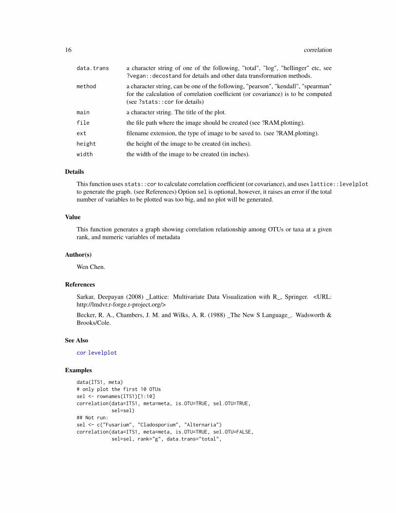
Usage

dissim.clust(elem, is.OTU=TRUE, stand.method=NULL,dist.method="morisita", clust.method="average")

dissim.eig(elem, is.OTU=TRUE, stand.method=NULL,dist.method="morisita")

dissim.ord(elem, is.OTU=TRUE, stand.method=NULL,dist.method="morisita", k=NULL)

dissim.GOF(elem, is.OTU=TRUE, stand.method=NULL,dist.method="morisita")

dissim.tree(elem, is.OTU=TRUE, stand.method=NULL,dist.method="morisita", clust.method="average")

dissim.pvar(elem, is.OTU=TRUE, stand.method=NULL,dist.method="morisita")

Arguments

elem an ecology data set that can be an OTU table or a taxonomy abundance table.See RAM.input.formatting for details.

is.OTU logical, whether the ecology data sets are OTU tables or taxonomy abundancematrices. See RAM.input.formatting for details.

stand.method optional, if is.null, the standardization method for data transforamtion; mustbe one of the following: "total", "max", "frequency", "normalize", "range","standardize", "pa", "chi.square", "hellinger", "log". See also decostand.

dist.method the dissimilarity index to be used; one of "manhattan", "euclidean", "canberra","bray", "kulczynski", "jaccard", "gower", "altGower","morisita", "horn","mountford", "raup", "binomial", "chao", or "cao". See also vegdist.

k the number of dimensions desired. If NULL, the maximum value will be calcu-lated and used.

clust.method the method used for clustering the data. Must be one of "ward", "single","complete", "average", "mcquitty", "median", or "centroid". See also hclust.

Value

dissim.clust returns a hierarchical clustering of the dissimilarity matrix.dist.eigenval returns the eigenvalues of the dissimilarity matrix.dissim.ord returns a list: the first item is the the ordination distances, the second is the

dissimilarity matrix distances.dissim.GOF returns the goodness of fit values of the dissimilarity matrix, for various numbers

of dimensions used.dissim.tree returns a list: the first item is the tree distances, the second is the dissimilarity

matrix distances.dissim.pvar returns a numeric vector containing the percent variation explained by each axis

(where each sample corresponds to an axis).

Author(s)

Wen Chen and Joshua Simpson

22 dissim.heatmap

See Also

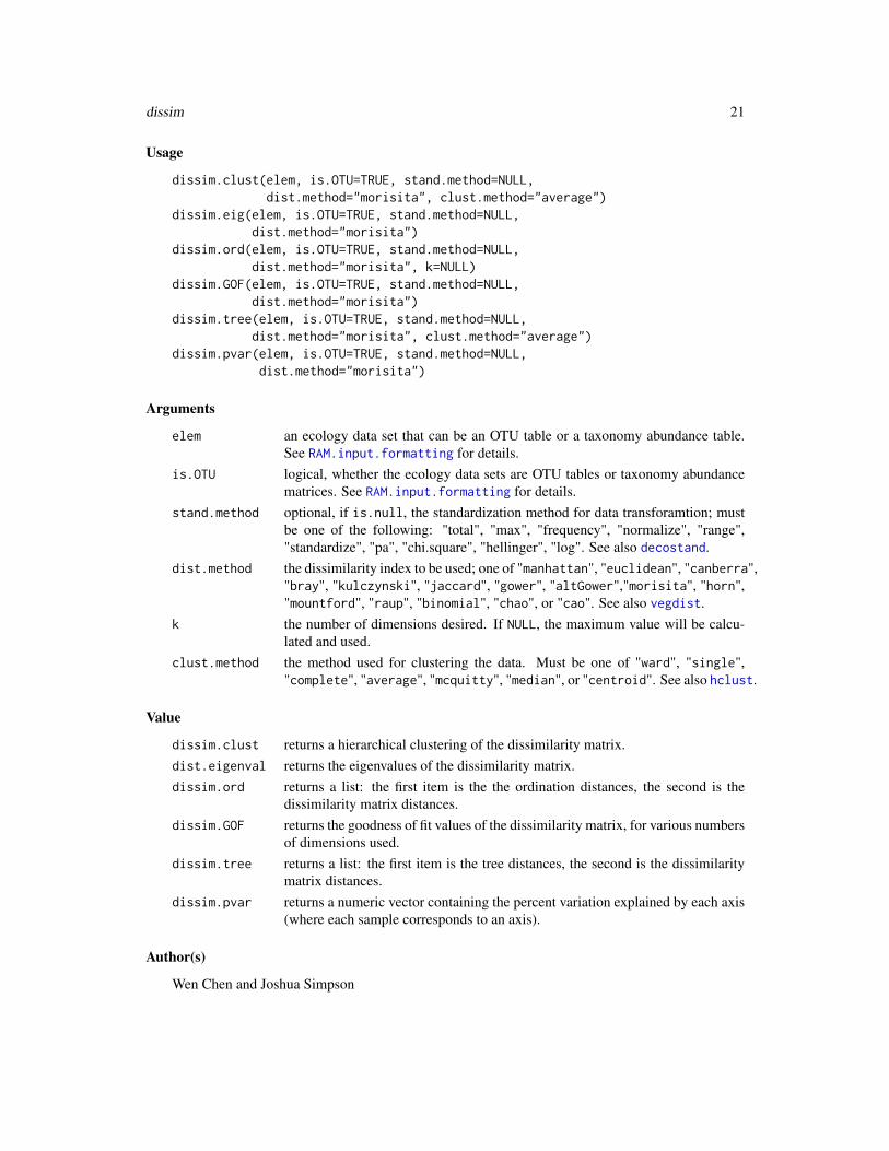
decostand, vegdist, hclust, dissim.plot

Examples

data(ITS1)# calculate clustering, using default methoddissim.clust(ITS1)# calculate tree distances, specifying a distance method# (but use default clustering method)dissim.tree(ITS1, dist.method="euclidean")# calcualte ordination distances, specifying both distance# and ordination methodsdissim.ord(ITS1, dist.method="bray", k=3)

dissim.heatmap Plot Distance Matrix Heatmap for OTU Samples

Description

This function consumes an OTU table, along with some optional parameters, and creates a heatmapshowing the distance matrix for the samples of the given OTU table.

Usage

dissim.heatmap(data, is.OTU=TRUE, meta=NULL, row.factor=NULL,col.factor=NULL, stand.method="chi.square",dissim.method="euclidean",file=NULL, ext=NULL, height=8, width=9,leg.x=-0.05, leg.y=0)

Arguments

data the OTU table to be used.



row.factor a factor from the metadata to show along the rows of the heatmap (see Detailsbelow).

col.factor a factor from the metadata to show along the columns of the heatmap (see Detailsbelow).

stand.method a method used to standardize the OTU table. One of "total", "max", "freq","normalize", "range", "standardize", "pa", "chi.square", "hellinger" or"log" (see ?decostand).

dissim.method the dissimilarity index to be used; one of "manhattan", "euclidean", "canberra","bray", "kulczynski", "jaccard", "gower", "altGower","morisita", "horn","mountford", "raup", "binomial", "chao", or "cao" (see ?vegdist).

dissim.heatmap 23


ext the file type to be used; one of "pdf", "png", "tiff", "bmp", "jpg", or "svg".



leg.x how far the legend should be inset, on the x axis.

leg.y how far the legend should be inset, on the y axis.

Details

Both row.factor and col.factor should be named character vectors specifying the names of therows to be used from meta (see RAM.factors). They should also be factors; if they are not, awarning is raised and they are coerced to factors (see factor). A warning is also raised when afactor has more than 8 levels, as that is the most colours the current palettes support. The factormust also correspond to the OTU table; i.e. they should have the same samples. If not, an error israised.

Note

This function creates the heatmap using the heatmap.2 function from the gplots package. Thatfunction calls layout to set up the plotting environment, which currently prevents plotting two datasets side by side, or to automatically place the (metadata) legend. Unfortunately, this means that theleg.x and leg.y parameters must be used to adjust the legend by trial and error. It is possible tomove the legend outside of the plotting area; if not legend appears, try with small leg.x and leg.yvalues.

Author(s)


See Also

decostand, vegdist, factor, heatmap.2, RAM.factors

Examples

data(ITS1, meta)# plot to the screen with one meta factor and standard# calculation methodsdissim.heatmap(ITS1, is.OTU=TRUE, meta=meta,

row.factor=c(Plot="Plots"))## Not run:# plot the heatmap to a .tiff file using Hellinger# standardization and Manhattan distancesdissim.heatmap(ITS1, dissim.method="manhattan",

stand.method="hellinger",file="my/sample/path", ext="tiff")

## End(Not run)

24 dissim.plot

dissim.plot Plot Dissimilarity Matrix Data for Different Methods

Description

These functions all produce a plot of some measure related to dissimilarity matrices. All of thesefunctions allow you to specify a vector of methods to be used when creating the plot.

Usage

dissim.clust.plot(data, is.OTU=TRUE, stand.method=NULL,dist.methods=NULL,clust.methods=NULL, file=NULL)

dissim.eig.plot(data, is.OTU=TRUE, stand.method=NULL,dist.methods=NULL, file=NULL)

dissim.alleig.plot(data, is.OTU=TRUE, stand.method=NULL,dist.methods=NULL, file=NULL)

dissim.ord.plot(data, is.OTU=TRUE, stand.method=NULL,dist.methods=NULL, k=NULL, file=NULL)

dissim.GOF.plot(data, is.OTU=TRUE, stand.method=NULL,dist.methods=NULL, file=NULL)

dissim.tree.plot(data, is.OTU=TRUE, stand.method=NULL,dist.methods=NULL,clust.methods=NULL, file=NULL)

dissim.pvar.plot(data, is.OTU=TRUE, stand.method=NULL,dist.methods=NULL, file=NULL)

Arguments

data a list of ecology data. See also RAM.input.formatting

is.OTU logical, whether the ecology data sets are OTU tables or taxonomy abundancematrices.

stand.method optional, if is.null, the standardization method for data transforamtion; mustbe one of the following: "total", "max", "frequency", "normalize", "range","standardize", "pa", "chi.square", "hellinger", "log". See also decostand.

dist.methods a character vector representing the dissimilarity indices to be used; each ele-ment must be one of one of "manhattan", "euclidean", "canberra", "bray","kulczynski", "jaccard", "gower", "altGower","morisita", "horn", "mountford","raup", "binomial", "chao", or "cao".

clust.methods a character vector representing the methods used for clustering the data. Each el-ement must be one of "ward", "single", "complete", "average", "mcquitty","median", or "centroid".

k the number of dimensions desired. If NULL, the maximum value will be calcu-lated and used.

file the file path for the plot. If not provided (defaults to NULL), then the plot isdisplayed to the screen. If file is provided, that is where the .tiff file will becreated.

dissim.plot 25

Details

All of these functions (other than dissim.alleig.plot) call dissim.X counterparts and plot thedata. If file is given, a .tiff file will be created at file; otherwise the plot is displayed to thescreen.

Value

All functions create a plot and return the plotted data invisibly.

dissim.clust.plot

plots a hierarchical clustering of the dissimilarity matrix.dissim.eig.plot

plots a bar plot of the eigenvalues of the dissimilarity matrix.dissim.alleig.plot

plots a line plot showing the relative importance of all eigenvalues for a varietyof methods.

dissim.ord.plot

plots a scatter plot comparing the "euclidean" distances among all samples inordination space to the dissimilarity matrix distances.

dissim.GOF.plot

plots a scatter plot of the goodness of fit values of the dissimilarity matrix, forvarious numbers of dimensions used.

dissim.tree.plot

plots a scatter plot comparing the tree distances to the dissimilarity matrix dis-tances.

dissim.pvar.plot

plots a bar plot showing the percent variation explained by each axis (whereeach sample corresponds to an axis).

Note

If file does not end in ".tiff", then ".tiff" will be appended to the end of file. Function dissim.alleig.plotuses the ggplot2 package for creating the plot, and returns the plot object. This means that you canstore this plot and add other features manually, if desired (see Examples).

Author(s)


See Also

vegdist, hclust, dissim, ggplot

Examples

data(ITS1, ITS2)data <- list(ITS1=ITS1, ITS2=ITS2)# show percent variation for only ITS1 with default methodsdissim.pvar.plot(data=list(ITS1=ITS1))

26 diversity.indices

## Not run:# show clustering for ITS1 and ITS2 for set methodsdissim.clust.plot(data=data, is.OTU=TRUE, stand.method=NULL,

dist.methods=c("morisita", "bray"),clust.methods=c("average", "centroid"))

dissim.ord.plot(data=data, is.OTU=TRUE, stand.method="total",dist.method="bray")

# dissim.alleig.plot returns a ggplot2 object:my.eig.plot <- dissim.alleig.plot(data)class(my.eig.plot) # returns "gg" "ggplot"my.eig.plot # view the plot# update the title, then view the updated plotmy.eig.plot <- my.eig.plot + ggtitle("My New Title")# update ggplot themerequire("grid")new_theme <-RAM.color()my.eig.plot <- my.eig.plot + new_thememy.eig.plot# save an image (named file.pdf) with GOF values for ITS1 and# ITS2, using default methodsdissim.GOF.plot(data=data, file="~/Documents/my/file")

## End(Not run)

diversity.indices Calculate True Diversity and Evenness

Description

These functions calculate true diversity and evenness for all samples.

Usage

true.diversity(data, index = "simpson")evenness(data, index = "simpson")

Arguments

data a list of otu tables to be processed. See RAM.input.formatting.

index the index to use for calculations; partial match to "simpson" or "shannon".

Details

For the following sections, S represents the number of species, λ represents the Simpson index, andH ′ represents the Shannon index.

The formulas for the true diversity of the indices are as follows:

• Simpson: D2 = frac1λ

• Shannon: D1 = expH ′

diversity.indices 27

The formulas for the evenness of the indices are as follows:

• Simpson:1λ

S

• Shannon: H′

lnS

Value

Both functions return a numeric data frame, where the rows are the given OTUs, and the columnsare the samples.

Note

Credit goes to package vegan for the partial argument matching (see References).

Author(s)


References

Jari Oksanen, F. Guillaume Blanchet, Roeland Kindt, Pierre Legendre, Peter R. Minchin, R. B.O’Hara, Gavin L. Simpson, Peter Solymos, M. Henry H. Stevens and Helene Wagner (2013). vegan:Community Ecology Package. R package version 2.0-10. http://CRAN.R-project.org/package=vegan

Diversity index. (2014, May 7). In Wikipedia, The Free Encyclopedia. Retrieved 14:57, May 28,2014, from http://en.wikipedia.org/w/index.php?title= Diversity_index&oldid=607510424

Blackwood, C. B., Hudleston, D., Zak, D. R., & Buyer, J. S. (2007) Interpreting ecological diversityindices applied to terminal restriction fragment length polymorphism data: insights from simulatedmicrobial communities. Applied and Environmental Microbiology, 73(16), 5276-5283.

Examples

data(ITS1, ITS2)# true diversity, using default index (Simpson)true.diversity(data=list(ITS1=ITS1))# true diversity for ITS1 and ITS2, using Shannontrue.diversity(data=list(ITS1=ITS1, ITS2=ITS2), index="shannon")# default evenness (Simpson) for ITS1/ITS2evenness(data=list(ITS1=ITS1, ITS2=ITS2))# Shannon evennessevenness(data=list(ITS1=ITS1), index="shannon")

28 envis.NB

envis.NB Visualize The Negative Binomial Model OF A Given Taxon OR OTUID

Description

This function plot the negative binomial model for a given otuID or taxon

Usage

envis.NB(NB.model="", tax.meta, taxon="",x="", num.col=NULL, group=NULL, group.order=NULL,xlab=NULL, ylab=NULL, fill=NULL, facet=NULL,file=NULL, ext=NULL, width=8, height=8)

Arguments

NB.model the negative binomial model. Can be obtained by using assist.NB

tax.meta the combined taxon/otuID and metadata. Can be obtained by using assist.NB

taxon the taxon or otuID. Can be obtained by using assist.NB

x a metadata variable name for x axis.

num.col optional. A metadata numerical variable that will be used as predictor.

group optional. A metadata factor variable that will be used as predictor.

group.order optional. The desired order for the group.

xlab optional. X axis label.

ylab optional. Y axis label.

fill optional. Color for fill different categories.

facet optional. Metadata category variables as faceting variables.


ext optional. Filename extension, type of image to be saved.

width an integer. Filter OTU table by counts.

height an integer. Filter OTU table by counts.

Value

This function plot predicted taxon/otuID under the impact of metadata variables.

Author(s)

Wen Chen

factor.abundance 29

Examples

data(ITS1, meta)# filter otu tableits1 <- filter.OTU(data=list(ITS1=ITS1), percent=0.01)[[1]]m <- meta[, c(2,3,5,7)]## Not run:# test the modelnb <- assist.NB(its1, meta=m, rank="g",

anov.fac="Harvestmethod",taxon=rownames(its1)[1])

NB.model<-nb[[1]]tax.meta<-nb[[2]]taxon<-nb[[3]]envis.NB(NB.model=NB.model, tax.meta=tax.meta, taxon=taxon,

x="Ergosterol_ppm", num.col="Ergosterol_ppm",group="Crop", group.order=NULL,xlab="Ergosterol (ppm)", ylab=NULL,fill="Harvestmethod", facet=c("City","Crop"))

## End(Not run)

factor.abundance Plot the Abundance of OTUs by Classification at a Given TaxonomicRank For Each Level of A Metadata Category Variable.

Description

This function consumes an OTU, and a rank, as well as various optional parameters. It creates astacked bar plot showing the abundance of all classifications at the given taxonomic rank for eachlevel of a metadata category variable.

Usage

factor.abundance(data, rank, top=NULL, count=FALSE,meta=meta, meta.factor="",drop.unclassified=FALSE, file=NULL,ext=NULL, height=8, width=16, main="")

Arguments

data a list of OTU tables with names.

rank the taxonomic rank to use. See RAM.rank.formatting.

top the number of groups to select, starting with the most abundant. If NULL, all areselected.

count logical. If TRUE, the numerical counts for each OTU will be shown; otherwisethe relative abundance will be shown.

meta metadata.

30 filter.META

meta.factor a category variable in metadata

drop.unclassified

logical. Should unclassified samples be excluded from the data?





main the title of the plot

Author(s)

Wen Chen

Examples

data(ITS1, ITS2, meta)data=list(ITS1=ITS1, ITS2=ITS2)# plot the relative abundance at the class level to the screen,# ignoring the unclassifiedfactor.abundance(data=data, rank="family", meta=meta,

meta.factor=c("Crop"), top=20,drop.unclassified=TRUE)

## Not run:# plot the count abundance at the phylum level to path.tifffactor.abundance(data=data, rank="family", meta=meta,

meta.factor=c("Crop"), top=20, count=FALSE,drop.unclassified=TRUE, main="",file="path/to/tiff", ext="tiff",height=8, width=12)

## End(Not run)

filter.META Select METADATA Variables

Description

This function will remove metadata variables with only one level and /or remove variables withmissing data or neither numeric nor factor/character (NNF).

Usage

filter.META(meta=meta, excl.na=TRUE, excl.NNF=TRUE,exclude=NULL)

filter.OTU 31

Arguments


excl.na logical. Whether or not remove variables that contain missing data.

excl.NNF logical. Whether or not remove variables that neither are numeric nor fac-tor/character.

exclude optional. If is NULL, the function only removes variables with only one level orNNF. Otherwise, the variables in the exclude will also be removed from themetadata table.

Value

The value returned by this function is a data frame with the following metadata variables beingremoved: 1) with missing data; 2) NNF if excl.NNF is TRUE; and 3) in the exclude list.

Author(s)

Wen Chen

Examples

data(meta)## Not run:# add a new column with NAmeta.nw <- metameta.nw$na <- c(rep(NA, nrow(meta.nw)-3), c(1, 3, 5))meta.nw$nf <- rep("Canada", nrow(meta.nw))meta.fil <- filter.META(meta.nw)meta.fil <- filter.META(meta.nw, excl.na=FALSE, excl.NNF=FALSE,

exclude=c("Province", "Latitude"))

## End(Not run)

filter.OTU Filter OTU

Description

This function filter OTU table by counts or relative abundance. If filter by counts, otus having totalcounts more than a threshhold will be kept. If filter by relative abundance, otus with the maximumrelative abundance greater than a threshhold in at least one subject will be kept.

Usage

filter.OTU(data, percent=NULL, number=NULL)

32 filter.Taxa

Arguments

data a list of otu tables to be processed. See also RAM.input.formatting

percent a floating point greater than 0 and less or equals to 1. Filter OTU table by relativeabundance.

number an integer. Filter OTU table by counts.

Value

The value returned by this function is a list of filtered otu tables provided by the user

Author(s)

Wen Chen

Examples

data(ITS1, ITS2, meta)data<-list(ITS1=ITS1, ITS2=ITS2)## Not run:otu.001 <- filter.OTU(data=data, percent=0.01)length(otu.001)names(otu.001)otu.50 <- filter.OTU(data=data, number=50)

## End(Not run)

filter.Taxa Filter Taxonomic Abundance Matrix by Total Counts Or MaximumRelative Abundance

Description

This function filter taxa group by counts or relative abundance. If filter by counts, taxa having totalcounts more than a threshhold will be kept. If filter by relative abundance, taxa with the maximumrelative abundance greater than a threshhold in at least one subject will be kept.

Usage

filter.Taxa(taxa, drop.unclassified=TRUE,percent=NULL, number=NULL)

Arguments

taxa the taxonomy abundance matrix: sample x species data frame. See also tax.abunddrop.unclassified

logical, whether or not remove unclassified groups. See also tax.abund

percent a floating point greater than 0 and less or equals to 1. Filter Taxa table by relativeabundance.

number an integer. FilterTaxa table by total sequence counts.

fread.meta 33

Value

The value returned by this function is a data frame with taxa met the filter requirement only.

Author(s)

Wen Chen

Examples

data(ITS1)g1 <- tax.abund(ITS1, rank="g", drop.unclassified=TRUE)taxa.fil <- filter.Taxa(g1, percent=0.01)

fread.meta Load Metadata Table

Description

This function is same as read.meta to read in data; except using fread for loading large data sets.

Usage

fread.meta(file, sep="auto")

Arguments

file a character vector specifying the file path to your file.

sep the character used to separate cells in the file.

Value

Returns a data frame with the information from the file. The first row and column are used for thenames of the other rows and columns.

Author(s)

Wen Chen

See Also

read.meta, fread

Examples

## Not run:my.meta <- fread.meta("path/to/meta")

## End(Not run)

34 fread.OTU

fread.OTU Fast Load Large OTU Table

Description

This function is same as read.OTU except using fread for loading large data sets.

Usage

fread.OTU(file, sep="auto")

Arguments



Value


Note

The OTU table should only contain classifications for the seven major taxonomic ranks, additionalranks will break some functions in the package. To remove those other classifications, try bashcommand sed -i.backup -e 's/s[a-z]__[^;]*; //g' -e 's/t__[^;]*; //g' $FILE where$FILE is your OTU table. The letter t can be replaced in the second expression for any other letterwhich appears as a prefix. For example, adding -e 's/u__[^;]*; //g' before $FILE wouldremove any entries formatted like u__test_classification; . Additionally, if your OTU tablestarts with the entry #OTU ID, that cell needs to be removed before the table can be read withfread.OTU.

Author(s)

Wen Chen.

See Also

read.OTU, fread

Examples

## Not run:my.OTU <- fread.OTU("path/to/otu")

## End(Not run)

get.rank 35

get.rank Get OTUs Classified at Taxonomic Rank(s)

Description

This function returns the OTUs of the given OTU table(s) which areclassified at the given taxonomicrank.

Usage

get.rank(otu1, otu2 = NULL, rank = NULL)

Arguments



rank a character vector representing a rank. Must be in one of three specific formats(see RAM.rank.formatting for help). If omitted, the function will repeat for allseven major taxonomic ranks.

Value

The value returned by this function may become nested lists, so for convenience, any nested listshave been given descriptive items names to make accessing its elements simple (see Examples).

• If otu2 is given:

– If rank is given: a list containing two data frames (otu1 and otu2 selected at the givenrank).

– If rank is not given: a list containing two lists. The first sublist represents otu1, thesecond otu2. The sublists contain seven data frames, which are the OTU tables selectedat each taxonomic rank (see Examples).

• If otu2 is not given:

– If rank is given: a single data frame (otu1 selected at the given rank).

– If rank is not given: a list containing seven data frames (otu1 selected at each taxonomicrank).

Author(s)


36 group.abund.Taxa

Examples

data(ITS1, ITS2)# the following are equivalent:ITS1.p <- get.rank(ITS1, rank="p")# this list has get.rank(ITS1, rank="k"),# get.rank(ITS1, rank="p"), ...lst <- get.rank(ITS1)stopifnot(identical(ITS1.p, lst$phylum))# true# get a list of length 2: the item holds all ITS1 data, the# second holds ITS2 datalst.all <- get.rank(ITS1, ITS2)stopifnot(identical(ITS1.p, lst.all$otu1$phylum))

group.abund.Taxa Barplot Of Distribution Of Taxa In Groups

Description

This function do a barplot to show the distribution of selected taxa in each level of a given metadatavariable

Usage

group.abund.Taxa(data, is.OTU=TRUE, rank="g", taxa,drop.unclassified=FALSE, bar.width=NULL,meta, meta.factor="", RAM.theme=NULL,col.pal=NULL, main="",file=NULL, ext=NULL, height=8, width=16)

Arguments

data a list of otu tables or taxonomic abundance matrices. See also RAM.input.formatting.


rank a single taxonomic rank. See also RAM.rank.formatting

taxa a vector containing taxa names for plotting.drop.unclassified

logical. Whether or not drop the unclassified taxon groups.

bar.width width of bars


meta.factor a character string. Must be one of the metadata variables.

RAM.theme customized ggplot_theme in RAM. See also ?theme_ggplot.

col.pal color palettes to be used.

main a character string. The title of the plot, default is an empty string.

group.abundance 37

file filename to save the plot.ext filename extension, the type of image to be saved to.width an integer, width of the plot.height an integer, height of the plot.

Value

This function returns a Barplot of the distribution of seleted taxa within each level of a given meta-data variable.

Note

This funtion provide an alternative view of taxa distribution as group.Taxa.bar.

Author(s)

Wen Chen.

Examples

data(ITS1, ITS2, meta)taxa <- c("Fusarium", "Alternaria", "Cladosporium")#otu tablesdata <- list(ITS1=ITS1, ITS2=ITS2)group.abund.Taxa(data=data, taxa=taxa, meta=meta,

meta.factor="Crop", drop.unclassified=TRUE)#abundance tablesITS1ab <- tax.abund(ITS1, rank="g")ITS2ab <- tax.abund(ITS2, rank="g")group.abund.Taxa(data=list(ITS1ab=ITS1ab, ITS2ab=ITS2ab),

is.OTU=FALSE, taxa=taxa,meta=meta, meta.factor="Crop",drop.unclassified=TRUE)

group.abundance Plot the Abundance of OTUs by Classification at a Given TaxonomicRank

Description

This function consumes an OTU, and a rank, as well as various optional parameters. It creates astacked bar plot showing the abundance of all classifications at the given taxonomic rank for eachsample.

Usage

group.abundance(data, rank,top=NULL, count=FALSE, drop.unclassified=FALSE,cex.x=NULL, main=NULL, file=NULL, ext=NULL,height=8, width=16, bw=FALSE, ggplot2=TRUE)

38 group.abundance

Arguments

data a list of OTU tables.




drop.unclassified


cex.x optional. The size of x axis names.






bw logical. Should the image be created in black and white?

ggplot2 logical. Should the ggplot2 package be used to produce the plot, or should thebase graphics be used? (see ?RAM.plotting).

Author(s)


Examples

data(ITS1, ITS2)# plot the relative abundance at the class level to the screen,# ignoring the unclassifiedgroup.abundance(data=list(ITS1=ITS1), rank="phylum",

drop.unclassified=TRUE)## Not run:# plot the count abundance at the phylum level to path.tiffgroup.abundance(data=list(ITS1=ITS1, ITS2=ITS2), rank="g",

top=10, count=FALSE, drop.unclassified=TRUE,main="", file=NULL, ext=NULL,height=8, width=16, bw=FALSE, ggplot=TRUE)

## End(Not run)

group.abundance.meta 39

group.abundance.meta Plot the Abundance of OTUs by Classification at a Given TaxonomicRank

Description

This function is an updated version of group.abundance, which groups samples by metadata cate-gory variables if provided.

Usage

group.abundance.meta(data, rank,top=NULL, count=FALSE, drop.unclassified=FALSE,cex.x=NULL, main=NULL, file=NULL, ext=NULL,height=8, width=16, bw=FALSE, meta=NULL,meta.factor=NULL)

Arguments





drop.unclassified









meta optional, associated metadata of the otu tables, sampleIDs and their orders inotu tables should be identical to those in metadata

meta.factor optional, category variables in meta

Author(s)

Wen Chen

40 group.diversity

Examples

data(ITS1, ITS2, meta)## Not run:# plot the relative abundance at the class level to the screen,# drop unclassified taxadata=list(ITS1=ITS1, ITS2=ITS2)group.abundance.meta(data, top=10, rank="family",

drop.unclassified=TRUE, meta=meta,meta.factor=c("Crop", "City"))

## End(Not run)

group.diversity Boxplot To Compare Diversity Indices Among Groups

Description

This function first use OTU.diversity to calculate the diversity indices for each sample and thendo a boxplot to compare the selected indices among different groups.

Usage

group.diversity(data, meta, factors="", indices="",diversity.info=FALSE,x.axis=NULL, compare=NULL,facet=NULL, facet.y=TRUE, facet.x.cex=NULL,facet.y.cex=NULL, scale.free=NULL,xlab=NULL, ylab=NULL,legend.title=NULL, legend.labels=NULL,file=NULL, ext=NULL, width=8, height=8)

Arguments

data a list, containing otu tables. See also RAM.input.formatting


factors a character vector. Must be variables in the metadata

indices a character vector. Must be one or more of the following: "spec", "sim", "in-vsim", "shan", "sim_even", "shan_even", "sim_trudiv", "shan_trudiv", "chao","ACE". See also OTU.diversity, true.diversity, evenness, and diversity.

diversity.info logical. Whether the diversity indices have calculated and included in the meta-data table. The diversity indices should be processed by OTU.diversity for thesame otu tables and metadata table.

x.axis optional. If NULL, will use the first variable in factors; otherwise, must be onefactor in the metadata or ’SampleID’

compare optional. If NULL, will use the first variable in factors; otherwise, must be onefactor in the metadata

group.diversity 41

facet optional. If provided, must be one factor in the metadata or ’SampleID’

facet.y logical, whether the facet being used as strip text of y axis or x axis.

facet.x.cex optional, an integer, the font size of the stip.text.x in ggplot

facet.y.cex optional, an integer, the font size of the strip.text.y in ggplot.

scale.free optional. Whether use free scale for y axis.

xlab optional. If not provided, the x.axis will be used as the title of the x axis,otherwise, will use the provided string.

ylab optional. If not provided, "value" will be used as the title of the y axis, otherwise,will use the provided string.

legend.title optional. If not provided, compare will be used as the title of the legend, other-wise, will use the provided string.

legend.labels optional. If not provided, will use the levels of compare for the legends, other-wise, will use the provided vector of strings. The length of the provided vectorof strings must equals to the levels of compare.

file the filename to save the plot.

ext the extention (file type) of the plot to saved.

width the width of the plot to be saved.

height the heigth of the plot to be saved.

Value

This function returns a boxplot to compared selected diversity indices among different groups.

Author(s)

Wen Chen.

See Also

OTU.diversity, true.diversity, evenness and diversity

Examples

data(ITS1, ITS2, meta)## Not run:RAM.theme<-RAM.color()group.diversity(data=list(ITS1=ITS1, ITS2=ITS2), meta=meta,

factors=c("Crop", "City"),indices=c("sim_trudiv", "shan_trudiv"),x.axis="Crop", compare="Harvestmethod",facet="City", facet.y=FALSE) + RAM.theme

## End(Not run)

42 group.heatmap

group.heatmap Plot OTU Abundance at a Given Rank with Metadata Annotation

Description

This function plots the abundance for all taxon groups at a given rank. Additionally, it can displaymetadata for the samples as annotations along the rows of the heatmap.

Usage

group.heatmap(data, is.OTU=TRUE, meta, rank, factors,top=25, remove.unclassified=TRUE,stand.method=NULL,dist.method="bray",hclust.method="average",dendro.row.status="yes",dendro.col.status="hidden",row.labels=TRUE, row.cex=1,cut=NULL, file=NULL, ext=NULL,width=9, height=9)

Arguments




rank the taxonomic rank to use (see RAM.rank.formatting for formatting details).

factors a named character vector indicating the columns of the metadata table to be used(see RAM.factors).


remove.unclassified

logical. Define whether OTUs labelled "unclassified" or missing classificationat the given taxonomic rank should be excluded.

stand.method optional. Data standardization methods specified in decostand.

dist.method distance matrix calculation methods specified vegdist.

hclust.method the agglomeration methods specified in hclust. This should be unambiguousabbreviation of one of the following: ’ward.D’, ’ward.D2’, ’single’, ’complete’,’average’, ’mcquitty’, ’median’ or ’centroid’.

dendro.row.status

whether or not to use the dendrogram to re-order the rows. It should be oneof the following: ’yes’ that use the dendrogram to re-order the rows/columnsand display the dendrogram; ’hidden’ means re-rorder, but do not display; ’no’means do not use the dendrogram at all. See also annHeatmap2

group.heatmap 43

dendro.col.status

whether or not to use the dendrogram to re-order the columns. It should be oneof the following: ’yes’ that use the dendrogram to re-order the rows/columnsand display the dendrogram; ’hidden’ means re-rorder, but do not display; ’no’means do not use the dendrogram at all. See also annHeatmap2

row.labels logical. Whether or not to plot the row labels.

row.cex the size of row labels if row.labels is TRUE

cut the height at which to cut the sample tree, this will create distinct colouredgroups. Currently this will allow for at most nine groups (see Details).





Details

A warning from brewer.pal indicating "n too large, allowed maximum for palette Pastel1 is 9"means that the cut height is too low to allow for that many groups. This should be fixed in a futurerelease.

Author(s)


See Also

decostand, annHeatmap2

Examples

data(ITS1, meta)## Not run:#library("Heatplus")#library("RColorBrewer")#group.heatmap(ITS1, is.OTU=TRUE, meta=meta, rank="c",

factors=c(Crop="Crop", City="City"),stand.method="chi", dist.method="euc",hclust.method="mcquitty", cut=0.5)

### End(Not run)

44 group.heatmap.simple

group.heatmap.simple Plot a Heatmap Showing OTU Abundance by Taxonomic Classifica-tion

Description

This function consumes an OTU table and a rank, as well as some optional parameters, and createsa heatmap showing the abundance of the OTUs at the given taxonomic rank for each sample.

Usage

group.heatmap.simple(data, is.OTU=TRUE, meta=NULL, rank,row.factor=NULL, top=NULL, count=FALSE,drop.unclassified=FALSE,dendro="none", file=NULL, ext=NULL,width=9, height=8, leg.x=-0.08, leg.y=0)

Arguments




rank the taxonomic rank to use (see ?RAM.rank.formatting for formatting details).

row.factor a factor from the metadata to show along the rows of the heatmap. (see Detailsbelow).

dendro a character vector specifying on which axes (if any) a dendrogram should beplotted. Must be one of "none", "both", "column", or "row".


count logical. Should the actual count of each OTU be shown, or should the relativeabundances be shown?

drop.unclassified

logical. Should OTUs labelled "unclassified" or missing classification at thegiven taxonomic rank be excluded?





leg.x how far the legend should be inset, on the x axis.

leg.y how far the legend should be inset, on the y axis.

group.indicators 45

Details

row.factor should be a named character vector specifying the name of the row to be used frommeta (see RAM.factors).

It should also be a factor; if it is not, a warning is raised and it is coerced to a factor (see factor).A warning is also raised when a factor has more than 8 levels, as that is the most colours the currentpalettes support. The factor must also correspond to the OTU table; i.e. they should have the samesamples. If not, an error is raised.

Note

This function creates the heatmap using the heatmap.2 function from the gplots package. Thatfunction calls layout to set up the plotting environment, which currently prevents plotting two datasets side by side, or to automatically place the (metadata) legend. Unfortunately, this means that theleg.x and leg.y parameters must be used to adjust the legend by trial and error. It is possible tomove the legend outside of the plotting area; if no legend appears, try with small leg.x and leg.yvalues.

Author(s)


See Also

factor, heatmap.2, RAM.factors

Examples

data(ITS1, meta)# plot the abundance of all observed classes for each sample,# displaying it to the screen and adding a dendrogram on the# column and the Collector on the rowgroup.heatmap.simple(ITS1, is.OTU=TRUE, meta=meta,

row.factor=c(Crop="Crop"), dendro="row",rank="g", top=10, drop.unclassified=TRUE,leg.x=-0.06)

## Not run:# plot the genus for all OTUs, add a dendrogram to the row and# column, and save the plot in path.tiffgroup.heatmap.simple(ITS1, is.OTU=TRUE, meta=meta, rank="genus",

dendro="both", file="my/file/path")## End(Not run)

group.indicators Plot Indicator Taxon Groups for Metadata Trends

Description

This function conumes one or two OTU tables, along with a metadata facotr, and creates a barplotshowing the relative abundance of all groups which are statistical indicators of that factor.

46 group.indicators

Usage

group.indicators(data, is.OTU=TRUE, meta, factor, rank,thresholds = c(A = 0.85,

B = 0.8,stat = 0.8,p.value = 0.05),

cex.x=NULL, file = NULL, ext = NULL,height = 12, width = 12)

Arguments

data a list of OTUs or taxonomic abundance matrices. see also RAM.input.formatting

is.OTU logical. Whether the input data are OTU tables.


factor a named character vector (of length 1) giving the name of the column in meta tobe used when performing the analysis (see RAM.factors).

rank the taxonomic rank to use (see ?RAM.rank.formatting for formatting details). ifrank is NULL, will use otus as indicators which are annotated by the lca assignedto the otus, otherwise will use taxon names as indicators at the given taxonomicrank.

thresholds a character vector of length 4 specifying the thresholds for the A, B, stat, and pvalues (see Details).






Details

This function uses indicspecies::multipatt to determine the indicators. After this analysis isperformed, there will likely be some species determined to be ’significant,’ but to varying degrees.To control how many groups are selected, you can adjust the thresholds argument. It consists offour components: (quotations taken from vignette("indicspeciesTutorial"), see References):

A the specificity of the indicator; ’the probability that the surveyed site belongs to the target sitegroup given the fact that the species has been found’

B the fidelity of the indicator; ’the probability of finding the species in sites belonging to the sitegroup’

stat the association strength for the combinations.

p.value ’the degree of statistical significance of the association’

Only the species with A, B, and stat values above, and p.value below those given in thresholdswill be kept.

group.OTU 47

Value

This function returns a stacked barplot and a vector of identified indicators, including the ones inthe plot and the ones being excluded from the plot.

Author(s)


References

De Caceres, M., Legendre, P. (2009). Associations between species and groups of sites: indices andstatistical inference. Ecology, URL http://sites.google.com/site/miqueldecaceres/

See Also

multipatt

Examples

data(ITS1, ITS2, meta)## Not run:# inputs are OTU tablesgroup.indicators(data=list(ITS1=ITS1, ITS2=ITS2), is.OTU=TRUE,

meta, factor = c(Province="Province"),rank="g")

group.indicators(data=list(ITS1=ITS1), is.OTU=TRUE, meta,factor = c(Province="Province"),rank=NULL)

group.indicators(data=list(ITS1=ITS1), is.OTU=TRUE, meta,factor = c(Province="Province"),rank=NULL)

# inputs are taxonomic abundance matricesg1 <- tax.abund(ITS1, rank="g")g2 <- tax.abund(ITS2, rank="g")group.indicators(data=list(g1=g1, g2=g2), is.OTU=FALSE, meta,

factor = c(Province="Province"),rank="g")

## End(Not run)

group.OTU Plot Distribution of OTUs

Description

This function plot the distributon of otus in each level of a given metadata variable. The plot canbe boxplot of barplot. The boxplot shows the range of relative abundance of a given otuID in eachlevel of metadata category. The barplot shows the relative abundance of the total counts of a givenotuID in each level of metadata category.

48 group.OTU

Usage

group.OTU(otu, rank="g", otuIDs="", meta, meta.factor="",boxplot=TRUE, main="", file=NULL, ext=NULL,height=8, width=16)

Arguments

otu the OTU table to be analyzed.

rank optional. if NULL, the lca of the OTUs will be retrieved; otherwise, the usershould provide a valid taxonomic rank that an otu being classified to (see ?RAM.rank.formattingfor formatting details).

otuIDs an vector of otuIDs in the OTU table



boxplot logical. If TRUE, generate boxplot; otherwise generate barplot.

main title of the plot.





Value

group.OTU returns boxplot or barplot for the distribution of a list of otuIDs.

Note


Author(s)

Wen Chen

See Also

ggplot

Examples

data(ITS1, meta)# otuIDsotuIDs=rownames(ITS1)[1:10]# names(meta)theme <- RAM.color()group.OTU(otu=ITS1, rank="g", otuIDs=otuIDs,

meta=meta, meta.factor="City", boxplot=TRUE,file=NULL, ext=NULL) + theme

group.rich 49

## Not run:group.OTU(otu=ITS1, rank="g", otuIDs=otuIDs,

meta=meta, meta.factor="City", boxplot=FALSE,file=NULL) + theme

## End(Not run)

group.rich Barplot Of Richness For Each Level Of A Given Metadata Variable

Description

This function first use specpool to estimate the extrapolated species richness in a species pool(levels of metadata variable), and the number of unobserved species, then do a barplot.

Usage

group.rich(otu, meta, factor, file=NULL, ext=NULL,width=8, height=8)

Arguments

otu an OTU table.


factor a character string. Must be one of the metadata variables.





Value

This function returns a barplot of species richness for a given metadata variable.

Author(s)

Wen Chen.

See Also

specpool, specpool

Examples

data(ITS1, meta)group.rich(ITS1, meta, "Crop")

50 group.spatial

group.spatial Plot Spatial Collection Trends for Taxon Groups

Description

This function consumes an OTU table and its associated metadata table, and uses that informa-tion to produce a choropleth (essentially a heatmap, but superimposed imposed on an actual, car-tographic map) to show how many counts of each taxon group were detected in each Canadianprovince/territory.

Usage

group.spatial(data, meta, date.col, province.col, rank, group,breaks = "year", file = NULL, ext = NULL,height = 8, width = 10)

Arguments



date.col a character vector specifying which column in metadata contains the date infor-mation (see RAM.dates).

province.col a character vector specifying which column in metadata contains the provinceinformation (see Details).

rank a character vector specifying the rank of the desired taxon groups. Note that allgroups should come the same rank. (see RAM.rank.formatting).

group a character vector giving the names of the groups to be plotted.

breaks how many time segments should be plotted; see Details.

file the file path where the image should be created. (see ?RAM.plotting).




Details

This function currently only supports Canadian data. The entries in meta$province.col should bespecified as provinces, using the standard postal abbreviations (e.g. "Ontario" would be "ON").

The breaks argument is slightly buggy at the moment, possibly due to how R tries to split Dateobjects. breaks can be either an integer, in which case it will attempt to create that many levels(i.e. setting breaks=3 should split the data into three date ’blocks’.) breaks can also be a charactervectors, such as "quarter" or "year" which attempts to split the date information accordingly. Seecut.Date for more details and a complete specification of what is allowed for breaks.

http://en.wikipedia.org/wiki/Canadian_postal_abbreviations_for_provinces_and_territories

group.spec 51

Author(s)


References

The file used to create the map of Canada is from GeoBase and is licensed under the Open Govern-ment License - Canada.

Examples

data(ITS1, meta)## Not run:group.spatial(ITS1, meta, date.col="Harvestdate",

province.col="Province", rank="p",group=c("Ascomycota", "Basidiomycota"),breaks=2)

## End(Not run)

group.spec Boxplot Of Richness For Each Level Of A Given Metadata Variable

Description

This function first use specpool to estimate the extrapolated species richness in a species pool(levels of metadata variable), and the number of unobserved species, then do a boxplot for percentof observed richness.

Usage

group.spec(otu, meta, factor, file=NULL, ext=NULL,width=8,height=8)

Arguments

otu an OTU table.


factor a character string. Must be one of the metadata variables.





Value

This function returns a boxplot of species richness for a given metadata variable.

http://www.geobase.ca/geobase/en/index.html

http://data.gc.ca/eng/open-government-licence-canada

http://data.gc.ca/eng/open-government-licence-canada

52 group.Taxa.bar

Author(s)

Wen Chen.

See Also

specpool, specpool

Examples

data(ITS1, meta)group.spec(ITS1, meta, "Crop")

group.Taxa.bar Barplot Of Taxa Distribution In Groups

Description

This function do a barplot to show the distribution of selected taxa in each level of a given metadatavariable

Usage

group.Taxa.bar(data, is.OTU=TRUE, rank="g", taxa="",meta, meta.factor="", func="sum", cex.y=5,cex.x=5, cex.main=10, bar.width=NULL,RAM.theme=NULL, col.pal=NULL, main="",file=NULL, ext=NULL, height=8, width=16)

Arguments




taxa a vector containing taxa names for plotting.



func function to be used to aggregate count data, e.g. "sum" or "mean", default is"sum"

cex.y size of y axis tick labels.

cex.x size of x axis tick labels.

cex.main size of title.

bar.width width of bars


group.Taxa.bar 53



file filename to save the plot.

ext filename extension, the type of image to be saved to.



Details

To use customized color palettes, must pass a vector of color names or hexadecimals. See examplesfor detail.

Value

This function returns a barplot.

Author(s)

Wen Chen

Examples

data(ITS1, ITS2, meta)taxa <- c("Fusarium", "Alternaria", "Cladosporium")group.Taxa.bar(data=list(ITS1=ITS1, ITS2=ITS2), is.OTU=TRUE,

rank="g", taxa=taxa, meta=meta,meta.factor="City", cex.y=5, cex.x=5,bar.width=1, RAM.theme=RAM.color())

## Not run:# change default color schemescol <- c("dodgerblue1", "darkcyan")taxa.1 <- c("Fusarium", "Alternaria", "Cladosporium",

"Verticillium", "Kondoa")group.Taxa.bar(data=list(ITS1=ITS1, ITS2=ITS2), is.OTU=TRUE,

rank="g", taxa=taxa.1, meta=meta,meta.factor="City", cex.y=5, cex.x=5,bar.width=1, RAM.theme=NULL, col.pal=col)

group.Taxa.bar(data=list(ITS1=ITS1, ITS2=ITS2), is.OTU=TRUE,rank="g", taxa=taxa.1, meta=meta,meta.factor="City", cex.y=5, cex.x=5,bar.width=1, RAM.theme=NULL,col.pal=col, func="mean")

# change ggplot themegroup.Taxa.bar(data=list(ITS1=ITS1, ITS2=ITS2), is.OTU=TRUE,

rank="g", taxa=taxa.1, meta=meta,meta.factor="City", cex.y=5, cex.x=5,bar.width=1, col.pal=col, RAM.theme=RAM.border())

# save the plotgroup.Taxa.bar(data=list(ITS1=ITS1, ITS2=ITS2), is.OTU=TRUE,

rank="g", taxa=taxa.1, meta=meta,

54 group.Taxa.box

meta.factor="City", cex.y=5, cex.x=5,bar.width=1, RAM.theme=NULL,col.pal=col,main="", file="path/to/filename.pdf",ext="pdf", height=8, width=16)

## End(Not run)

group.Taxa.box Boxplot Of Taxa In Each Level of A Metadata Variable

Description

This function do a boxplot to show the distribution of selected taxa in each level of a given metadatavariable

Usage

group.Taxa.box(data, is.OTU=TRUE, rank="g",taxa="", meta, meta.factor="",cex.y=5, cex.x=5, cex.main=10,RAM.theme=NULL, col.pal=NULL, main="",file=NULL, ext=NULL, height=8, width=16)

Arguments




taxa a vector containing taxa names for plotting.



cex.y size of y axis tick labels.

cex.x size of x axis tick labels.

cex.main size of title.








group.temporal 55

Value

This function returns a boxplot of the distribution of seleted taxa within each level of a given meta-data variable.

Author(s)

Wen Chen.

Examples

data(ITS1, ITS2, meta)taxa <- c("Fusarium", "Alternaria", "Cladosporium")group.Taxa.box(data=list(ITS1=ITS1, ITS2=ITS2),

is.OTU=TRUE, rank="g",taxa=taxa, meta=meta, meta.factor="City")

## Not run:taxa.1 <- c("Fusarium", "Alternaria", "Cladosporium",

"Verticillium", "Kondoa")group.Taxa.box(data=list(ITS1=ITS1, ITS2=ITS2),

is.OTU=TRUE, rank="g",taxa=taxa.1, meta=meta, meta.factor="City")

## End(Not run)

group.temporal Plot Temporal Trends for Metadata and Taxon Groups

Description

This function consumes an OTU table and its associated metadata, and creates a plot showing howthe collections of taxonomic groups, as well as metadata factors, evolve over time.

Usage

group.temporal(data, meta, date.col, factors, rank, group,file = NULL, ext = NULL, height = 8, width = 12)

Arguments



date.col a character vector specifying which column of the metadata has date information(see RAM.dates).

factors a named character vector specifying the names of the metadata columns to beplotted with the taxon group data. (see RAM.factors). NOTE: these factorsmust be numeric variables.

56 group.venn

rank a character vector specifying the rank of the desired taxon groups. Note that allgroups should come the same rank. (see RAM.rank.formatting).

group a character vector giving the names of the groups to be plotted.





Details

The image created will contain several plots. It will always contain a large panel showing the countscollected for the specified taxon groups over time, and above that panel (on a common x-axis) willbe a line graph for each metadata factor specified.

Note

If your data has collections being taken roughly annually, you may have a large amount of "emptyspace" in the middle of your plot. Consider subsetting the data by year, and plotting each yearindividually using this function.

Author(s)


Examples

data(ITS1, meta)group.temporal(ITS1, meta, date.col="Harvestdate",

factors=c(Ergosterol="Ergosterol_ppm"),rank="p", group=c("Ascomycota", "Basidiomycota"))

group.venn Plot Venn Diagram For Two To Five Sets With Item Labels

Description

This function use draw.pairwise.venn to creates a venn diagram for two vectors

Usage

group.venn(vectors, cat.cex=1.5, cex=1,cat.pos=NULL, cat.dist=NULL,label=TRUE, lab.cex=1,lab.col= "black", fill=NULL,file=NULL, ext=NULL, width=8, height=8)

group.venn 57

Arguments

vectors a list of vectors with names. See also RAM.input.formatting.

cat.cex size of the category names. (see venn.diagram for details).

cex size of the label of the circles. (see venn.diagram for details).

cat.pos optional. Location of the category names along the circles. (see venn.diagramfor details).

cat.dist optional. Distance of the category names to the circles. (see venn.diagram fordetails).

label logical. If TRUE, will plot the item labels for 2 data sets. For more than 2datasets or this is set as FALSE, the labels will be numbers for each circle. (seevenn.diagram for details).

lab.cex size of the labels.

lab.col color of the labels.

fill optional, color of the circles. (see venn.diagram for details).





Value

group.venn returns a venn diagram for 2 to 5 sets. The user can choose to place item labels for 2sets of data, however, the label locations can be wrong if the the smaller data set is part of the biggerdata set, in this case, set label as FALSE. If the input datasets is more than 2, label will be ignored.

Author(s)

Wen Chen

See Also

see venn.diagram

Examples

data(ITS1, meta)# core OTUscore <- core.OTU.rank(data=list(ITS1=ITS1), meta=meta, rank="g",

meta.factor="Crop", percent=1)# taxa that core OTUs assigned tocore.Crop1 <- core$ITS1$Crop1$taxacore.Crop2 <- core$ITS1$Crop2$taxa# venn plotvectors <- list(Core_Crop1=core.Crop1, Core_Crop2=core.Crop2)group.venn(vectors=vectors, label=TRUE, cat.pos=c(330, 150),

lab.cex=0.7)

58 ITS1/ITS2

## Not run:group.venn(vectors=vectors, label=FALSE, cat.pos=c(330, 150),

lab.cex=0.7, cex=3)

## End(Not run)

ITS1/ITS2 Sample ITS1 and ITS2 Data

Description

Sample ITS1 and ITS2 OTU tables.

Usage

data(ITS1)data(ITS2)

Format

A data frame with 4704 observations on the following 17 variables.

P1001.1M1, P1001.1M2, P1001.1M3, P1001.1M4, P1001.1M5, P1001.1M6, P1001.1M7, P1001.1M8, P1001.1M9, P1001.1M10, P1001.1M11, P1001.1M12, P1001.1M13, P1001.1M14, P1001.1M15, P1001.1M16Collection samples.

taxonomy the taxonomic classification of the OTU.

Source

Wen Chen, AAFC-AAC

Examples

data(ITS1, ITS2)str(ITS1)str(ITS2)

LCA.OTU 59

LCA.OTU Lowest Common Ancestor (LCA) OF EACH OTU

Description

This function consumes an OTU table and extract the LCA (lowest common ancestor) that each otuassigned to. See also tax.split.

Usage

LCA.OTU(otu, strip.format=FALSE, drop=TRUE)

Arguments

otu the OTU table to be used.

strip.format logical. Whether or not to remove the prefix of the taxonomy assignment at eachrank. see

drop logical. Whether or not drop taxonomic columns other than LCA.

Value

This function return a data frame same as the input OTU table, except the last column is the LCAof each otu, not the lineage. The taxonomy column can be kept, by using drop.

Note

tax.split returns the same OTU table with classification at a given taxonomic rank, which canbe missing if an otu was not classified a that that taxonomic level. LCA.OTU, guaranteed that allOTUs will be preserved in the returned data table and provide the LCA for each OTU, althoughonly higher taxonomic ranks were available.

Author(s)

Wen Chen

See Also

tax.split

Examples

data(ITS1)## Not run:# compare the following 2 commands:# keep the rank prefix of the LCA columnITS1.LCA <- LCA.OTU(ITS1, strip.format=TRUE, drop=TRUE)# remove the rank prefix of the LCA columnITS1.LCA <- LCA.OTU(ITS1, strip.format=FALSE, drop=TRUE)

60 location.formatting

## End(Not run)

location.formatting Location Formatting

Description

Some functions in RAM expect to find a column with provincial/territorial data in the metadata. Thisdata should use the standard Canadian provincial/territorial abbreviations:

• Alberta - AB

• British Columbia - BC

• Manitoba - MB

• New Brunswick - NB

• Newfoundland and Labrador - NL

• Novia Scotia - NS

• Northwest Territories - NT

• Nunavut - NU

• Ontario - ON

• Prince Edward Island - PE

• Quebec - QC

• Saskatchewan - SK

• Yukon - YT

Support for other locations is not available at this time.

Author(s)


match.data 61

match.data Match Samples In Ecology Data Sets and Metadata

Description

This function will match samples in ecology data sets, either OTU tables or taxonomy abundancematrices, and those in metadata. It makes sure that datasets contains same samples in the sameorder.

Usage

match.data(data, is.OTU=TRUE, meta)

Arguments

data a list of ecology data sets. if is.OTU is TRUE, they should be OTU tables, other-wise should be taxonomy abundance matrices. See also RAM.input.formatting.

is.OTU logical, whether or not the ecology data sets are OTU tables.

meta metadata associated with input ecology data sets.

Author(s)

Wen Chen

See Also

RAM.input.formatting

Examples

## Not run:data(ITS1, ITS2, meta)meta <- meta[1:8, ]# use otu tablesmatched <- match.data(data=list(otu_ITS1=ITS1, otu_ITS2=ITS2),

is.OTU=TRUE, meta=meta)# use taxonomy abundance matricesg1 <- tax.abund(ITS1, rank="g")g2 <- tax.abund(ITS2, rank="g")matched <- match.data(data=list(genus_ITS1=g1, genus_ITS2=g2),

is.OTU=FALSE, meta=meta)# class(matched)# names(matched)

## End(Not run)

62 meta

meta Sample Metadata for ITS1/ITS2

Description

This data frame provides sample metadata for the ITS1/ITS2 data included in this package.

Usage

data(meta)

Format

A data frame with 16 observations on the following 10 variables.

Sample a factor with levels Sample1 Sample2 Sample3 Sample4 Sample5 Sample6 Sample7 Sample8

City a factor with levels City1 City2

Crop a factor with levels Crop1 Crop2

Plots a factor with levels 1 2

Harvestmethod a factor with levels Method1 Method2

Harvestdate a Date

Ergosterol_ppm a numeric vector

Province a character vector

Latitude a numeric vector

Longitude a numeric vector

Source


Examples

data(meta)str(meta)

META.clust 63

META.clust Plot Hierarchical Cluster Of Metadata

Description

This function plot hierarchical cluster Of metadata.

Usage

META.clust(meta, group=4, data.trans=NULL, dist=NULL,clust=NULL, type=NULL, main="", file=NULL,ext=NULL, width=8, height=8)

Arguments

meta the metadata table to be clustered.

group an integer or a metadata variable. If an integar, will cut tree into correspondinggroups and color them accordingly; if a metadata variable was provided, treeleaves (sampleIDs) will be colored by each level.

data.trans optional. If provided, numeric data will be transformed. See also decostand

dist optional. If provided, distance matrix will be calculated using the give methodfor numeric variables; otherwise use vegdist default Bray-Curtis method. Ifmetadata include qualitative variables, distance matrix will be calculated bygowdis.

clust optional. If not provided, will use the default agglomeration method used byhclust, i.e. "complete". Otherwise, will used user defined method for clustering.See also hclust.

type optional. Can be one of the following: "triangle", "rectangle", "phylogram","cladogram", "fan", "unrooted", "radial".



ext optional. File type that the plot to be saved to.



Value

This function return a plot of the hierarchical cluster analysis on a set of metadata.

Author(s)

Wen Chen

64 network_data

See Also

vegdist and gowdis.

Examples

data(meta)META.clust(meta=meta, type="fan")META.clust(meta=meta, type="fan", group="City")META.clust(meta=meta, type="rectangle", group="Harvestmethod")META.clust(meta=meta, type="triangle", group="City",

clust="average")

network_data Creates Nodes and Edge-List For An OTU Table

Description

This function creates nodes and edge-list for an otu table, which can be used for network plotting

Usage

network_data(data, is.OTU=TRUE, metadata)

Arguments

data an otu table of a species abundance matrix

is.OTU whether or not data is an otu table

metadata associated metadta of the otu table, should have same sampleIDs

Value

Return a list of network nodes and edges based on an otu table and the associated metadata

Author(s)

Wen Chen

Examples

data(ITS1, meta)## Not run:ITS1.01<-filter.OTU(data=list(ITS1=ITS1), percent=0.01)[[1]]

# create nodes and edges listsb<-network_data(ITS1.01, is.OTU=TRUE, meta)b_node<-b[[1]]b_edge<-b[[2]]head(b_node)

OTU.diversity 65

head(b_edge)

library(igraph)b1<-graph.data.frame(b_edge, directed=FALSE)lev <- levels(factor(E(b1)$Crop))

# vertices sizeV(b1)$size<-degree(b1)

# vertices colorCrop1<-rownames(meta)[meta$Crop=="Crop1"]Crop2<-rownames(meta)[meta$Crop=="Crop2"]

## vertices representing samples from crop1 will be in red,## vertices representing samples from crop2 will be in blue;## vertices representing taxa will be in pinkV(b1)$color[which(is.element(V(b1)$name, Crop1))]<-"red"V(b1)$color[which(is.element(V(b1)$name, Crop2))]<-"blue"V(b1)$color[-which(is.element(V(b1)$name, c(Crop1, Crop2)))]<-"pink"V(b1)$color

# edges colorcol<-c("red", "blue")for (i in 1:length(lev) ) {

E(b1)$color[E(b1)$Crop==lev[i]] <- col[i]}

# plotplot(b1, vertex.label.font=2,

vertex.label.cex=0.5,layout=layout.kamada.kawai)

## End(Not run)

OTU.diversity Summarize Diversity Indices for OTU Tables

Description

These functions calculate diversity indices for all samples and append outputs as new columns tometadata table.

Usage

OTU.diversity(data, meta)

Arguments


meta the metadata to append the outputs.

66 OTU.ord

Details

This function summarize the following diversity indices: specnumber, shannon, simpson, invsimp-son, true diversity, evenness, chao and ACE indices, for a given otu table. See diversity.indices)

Value

This function return vectors of diversity indices for each sample, which are appended to a givenmetadata table.

Note

Credit goes to package vegan for the partial argument matching (see References), and for the cal-culation of all diversity indices except for true diversity and evenness.

Author(s)

Wen Chen.

References

Jari Oksanen, F. Guillaume Blanchet, Roeland Kindt, Pierre Legendre, Peter R. Minchin, R. B.O’Hara, Gavin L. Simpson, Peter Solymos, M. Henry H. Stevens and Helene Wagner (2013). vegan:Community Ecology Package. R package version 2.0-10. http://CRAN.R-project.org/package=vegan

Diversity index. (2014, May 7). In Wikipedia, The Free Encyclopedia. Retrieved 14:57, May 28,2014, from http://en.wikipedia.org/w/index.php?title= Diversity_index&oldid=607510424

Blackwood, C. B., Hudleston, D., Zak, D. R., & Buyer, J. S. (2007) Interpreting ecological OTU.diversityapplied to terminal restriction fragment length polymorphism data: insights from simulated micro-bial communities. Applied and Environmental Microbiology, 73(16), 5276-5283.

Examples

data(ITS1, ITS2, meta)data=list(ITS1=ITS1, ITS2=ITS2)## Not run:meta.diversity<-OTU.diversity(data=data, meta=meta)

## End(Not run)

OTU.ord Ordination Plot For OTUs Using CCA or RDA Analysis

Description

This function consumes an OTU table, metadata factors, and graphing options, then produces a plotshowing the cca or rda analysis of the OTU table.

OTU.ord 67

Usage

OTU.ord(otu, meta=meta, factors=NULL, group=NULL,na.action=c("na.fail", "na.omit", "na.exclude"),rank="g", taxa=NULL, data.trans="total",plot.species=TRUE, plot.scaling=-1,biplot.scale=NULL, biplot.sig=NULL, biplot.label= TRUE,mode=c("rda", "cca"), choice=c(1,2),main="", cex.point=3, cex.leg=12, cex.bp=3,file=NULL, ext=NULL, width=10, height=10)

Arguments

otu the OTU table to be used.meta the metadata table to be used.factors a named character vector of length 1 or 2 specifying metadata factors for the

samples in the OTU table (see Details).group a named character vector of length 1 or 2 specifying metadata factors for the

samples in the OTU table (see Details).na.action choice of one of the following: "na.fail", "na.omit" or "na.exclude", see na.action

in cca for detail.rank the rank to select the taxon groups at.taxa an integer or a character vector of taxa names at the given rank. If it’s an integer,

will display the top most abundant taxa; if it’s a vector of taxa names, will plotthe selected taxa.

data.trans a method used to standardize the OTU table. One of "total", "max", "freq","normalize", "range", "standardize", "pa", "chi.square", "hellinger" or"log" (see ?decostand).

plot.species whether plot sites or taxa, should be reflex to plot.scaling

plot.scaling one of the following: 1, 2, 3, or -1. See scaling in plot.cca for detail. Seealso ordiplot

biplot.scale a numeric number, length of the biplot arrowsbiplot.sig significance cutoff for biplot to be displayed. Currently disabled because in the

function, calculated ordination model cannot be passed to anova test.biplot.label whether or not to plot biplotmode one of the following: "cca" or "rda".choice the chosen axesmain title of the plotcex.point size of pointscex.leg size of lengend namecex.bp size of biplot labelsfile the file path where the image should be created (see ?RAM.plotting).ext the file type to be used; one of "pdf", "png", "tiff", "bmp", "jpg", or "svg".width the width of the image to be created (in inches).height the height of the image to be created (in inches).

68 OTU.rarefy

Details

group should be a named character vector specifying the names of the columns to be used frommeta (see RAM.factors). The values on the axes denote what fraction of the sum of all eigenvalues(i.e. from all axes) is explained by that (single) axis.

Value

return a list of following: 1) ggplot object; 2) ordination model; 3) commodity data and 4) metadataused for the ordination model.

Author(s)

Wen Chen.

See Also

decostand, Taxa.ord, pcoa.plot

Examples

data(ITS1, meta)its1<- filter.OTU(data=list(ITS1=ITS1), percent=0.001)[[1]]factors=c("City", "Crop", "Harvestmethod", "Ergosterol_ppm")## Not run:# plot sitesord1 <- OTU.ord(its1, meta=meta, data.trans="total",

factors=factors, mode="cca", biplot.sig=0.1,taxa=20, biplot.scale=1.5, cex.point=5,plot.species=FALSE, rank="f", plot.scaling=3,group=c(City="City", Crop="Crop"))

# plot taxaord2 <- OTU.ord(its1, meta=meta, data.trans="total",

plot.scaling=-1,factors=factors, mode="cca", biplot.sig=0.1,taxa=20, biplot.scale=3, cex.point=3,plot.species=TRUE, rank="g")

## End(Not run)

OTU.rarefy Create Rarefied OTU Tables

Description

This function output rarefied OTU tables using rrarefy. This function may take long time for largedataset, e.g. over 100k otus x 45 samples.

OTU.recap 69

Usage

OTU.rarefy(data, sample=NULL)

Arguments

data a list of otu tables. See also RAM.input.formatting.

sample an integer represent the sampling size.

Value

This function returns a list of rarefied otu tables.

Note

See also rrarefy

Author(s)

Wen Chen

See Also

RAM.input.formatting.

Examples

## Not run:data(ITS1, ITS2)otus.rf <- OTU.rarefy(data=list(ITS1=ITS1, ITS2=ITS2),

sample=NULL)

## End(Not run)

OTU.recap Summarize OTU

Description

This function summarize OTU table at each given taxonomic ranks.

Usage

OTU.recap(data, ranks=c("p", "c", "o", "f", "g"),brewer.pal="Pastel1", file=NULL, ext="pdf",width=12, height=8)

70 OTU.recap

Arguments

data a list of otu tables. See also RAM.input.formatting.

ranks a vector of taxonomic ranks. See also RAM.rank.formatting

brewer.pal one of the color patterns available in RColorBrewer. See brewer.pal for avail-able selections.


ext extention of the filename to save the plot.

width width of the plot

height heigth of the plot

Value

This function returns either a data frame or a list of data frames. If a single otu was provided, itreturns the a dataframe with information of how many otuIDs and sequences being classified atselected taxonomic ranks. If more than 1 otu tables being provided, it returns a list, with the first afew are data frames of classification summary of each otu table, the last is a list showing taxa foundonly in one of the otu data set. This function also generates a barplot for the percent classified otusand sequences at each given rank.

Note

warning is raised when run strsplit() and can be ignored.

Author(s)

Wen Chen

See Also

RAM.rank.formatting and RAM.input.formatting.

Examples

data(ITS1, ITS2)ranks <- c("p", "c", "o", "f", "g")df <- OTU.recap(data=list(ITS1=ITS1, ITS2=ITS2), ranks=ranks)class(df)

pcoa.plot 71

pcoa.plot Create a PCoA plot for an OTU Table

Description

This function consumes an OTU table, metadata factors, and graphing options, then produces a plotshowing the PCoA analysis of the OTU table.

Usage

pcoa.plot(data, is.OTU=TRUE, meta, factors, rank,stand.method = NULL, dist.method = "morisita",sample.labels = TRUE, top = 20,ellipse = FALSE, main = NULL, file = NULL, ext = NULL,height = 8, width = 10, ggplot2 = TRUE, bw = FALSE)

Arguments

data an OTU table or taxonomic abundance matrix to be used.

is.OTU logical. Whether or not the input data an OTU table.


factors a named character vector of length 1 or 2 specifying metadata factors for thesamples in the OTU table (see Details).

rank the rank to select the taxon groups at. For an OTU table, if rank is set NULL,distance matrix will be calcuated using all OTUs, otherwise, the OTU table willbe transformed to taxonomic abundance matrix before the calculation of thedistance matrix. If a taxonomic abundance matrix is provided, i.e. is.OTU is setTRUE, then the rank will be ignored.

stand.method a method used to standardize the OTU table. One of "total", "max", "freq","normalize", "range", "standardize", "pa", "chi.square", "hellinger" or"log" (see ?decostand).

dist.method the dissimilarity index to be used; one of "manhattan", "euclidean", "canberra","bray", "kulczynski", "jaccard", "gower", "altGower","morisita", "horn","mountford", "raup", "binomial", "chao", or "cao" (see vegdist).

sample.labels logical. Should the labels for the samples be displayed?

top how many taxon groups should be displayed, starting from the most abundant.

ellipse which of the metadata factors (if any) should have ellipses plotted around them.Must be one of 1, 2, or FALSE (see Details).






72 pcoa.plot



Details

This function uses pco in the labdsv package for the Principal coordinates analysis (PCoA). The dis-tance matrix was square rooted before being passed to pco to avoid negative eigenvalues. factorsshould be a named character vector specifying the names of the columns to be used from meta (seeRAM.factors). Those columns should be factors; if they are not, a warning is raised and they arecoerced to factors (see factor). A warning is also raised when a factor has more than 9 levels, asthat is the most colours the current palettes support.

The values on the axes denote what fraction of the sum of all eigenvalues (i.e. from all axes)is explained by that (single) axis. When ellipse = FALSE, no ellipses will be plotted. Whenellipse is a number, that ’number’ metadata factor will have ellipses plotted.

For example, if factors = c(Crop="Crop", City="City") and ellipse = 1, ellipses willbe plotted for the different crops, but NOT the cities. Setting factors = c(City="City") andellipse = 2 is invalid, since there is no second metadata factor given. Ellipses can only be plottedfor one factor currently. Furthermore, there need to be at least 3 samples for every level in everyitem in factors, otherwise ellipses cannot be plotted.

Value

When ggplot2 = TRUE, a ggplot object is returned; otherwise nothing ism returned (but the plot isshown on screen).

Note

The labels for the sample points are placed above, below, or next to the point itself at random. Iflabels are outside of the plotting area, or overlapping with each other, run your command again(without changing any arguments!) and the labels should move to new positions. Repeat until theyare placed appropriately. This is done to ensure even tightly-grouped samples, or samples near theedge of the plot, have their labels shown. If the labels are too distracting, remember that they canbe turned off by setting sample.labels = FALSE.

Author(s)


See Also

vegdist

Examples

data(ITS1, meta)# The argument for factors is a vector of length two; the first# item is # Crop, which is a column from meta, and the second# item is City, another # column from meta.

percent.classified 73

pcoa.plot(ITS1, meta=meta, rank="c",factors=c(Crop="Crop", City="City"))

## Not run:# If you want to customize legend labels and plot the top 20# taxon groups at genus:pcoa.plot(ITS1, meta=meta, rank="g", main="PCoA plot",

factors=c(Place="City",Harvest_Method="Harvestmethod"))

# In black & white, using base graphics:pcoa.plot(ITS1, meta=meta, rank="c", factors=c(Plot="Plots"),

ggplot=F, bw=T)pcoa.plot(ITS1, meta=meta, rank="c", factors=c(Plot="Plots"),

ggplot=F, bw=T, dist.method="euc",stand.method="hell")

# Focus on the samples: hide all groups and plot ellipses# for Crop:pcoa.plot(ITS1, meta=meta, rank="g",

factors=c(Crop="Crop", City="City"),ellipse=1, sample.labels=FALSE, top=0)

# Standardize the data before calculating distances:pcoa.plot(ITS1, meta=meta, rank="g", factors=c(City="City"),

stand.method="chi.square",dist.method="euclidean")

## End(Not run)

percent.classified Calculate Percent of OTUs Classified at a Given Taxonomic Rank

Description

This function consumes an OTU table, and a vector containing taxnomic ranks, then returns whatpercent of OTUs in the given table are classified at each taxonomic rank.

Usage

percent.classified(data, ranks=c("f","g"))

Arguments

data a list of OTU tables to be processed. See also RAM.input.formatting

ranks a vector containing the taxonomic ranks you are interested in (see ?RAM.rank.formattingfor formatting details).

Value

A list of numeric vectors, containing the result for each taxonomic rank.

74 phylog_taxonomy

Author(s)


Examples

data(ITS1, ITS2)data <- list(ITS1=ITS1, ITS2=ITS2)# find what percent of OTUs classified at family and genus# levelspercent.classified(data=data, ranks=c("f","g"))

phylog_taxonomy Plot Hierarchical Taxonomic Tree

Description

This function plots hierarchical taxonomic tree, the leaves are taxa at a give rank, nonsplitting nodesare not collapsed as ape::plot.phylo does.

Usage

phylog_taxonomy(otu, rank="order", rank.sep="; ", meta,factors=NULL, sel.taxon=NULL, sel.rank=NULL,root="root", cleaves=1, cnodes=1,clabel.leaves = 0.5, clabel.nodes = 0.5,f.phylog = 0.5, sub = TRUE, csub = 1.25,possub = "bottomleft", draw.box = TRUE)

Arguments

otu an otu table.


rank.sep the delimiter that separate the taxonomic ranks in the otu table; default is "; "(semi colon and a white space)

meta the metadata table associated with otu table, samples must be in the same orderin both otu table and metadata.

factors the metadata variables, must be categories

sel.taxon optional, a selected taxon at higher taxonomic rank (i.e. at phylum level). Ifgiven, only descendents of this taxa will be plotted.

sel.rank the rank of sel.taxon

root optional, the name of the root of the tree. If not given, will use "root"

cleaves see ?ade4::plot.phylog

phylo_taxonomy 75

cnodes see ?ade4::plot.phylog

clabel.leaves see ?ade4::plot.phylog

clabel.nodes see ?ade4::plot.phylog

f.phylog see ?ade4::plot.phylog

sub see ?ade4::plot.phylog

csub see ?ade4::plot.phylog

possub see ?ade4::plot.phylog

draw.box see ?ade4::plot.phylog

Author(s)

Wen Chen

Examples

data(ITS1, meta)## Not run:ITS1.1<-filter.OTU(data=list(ITS1=ITS1), percent=0.01)[[1]]factors=c("Crop", "City")phylog_taxonomy(otu=ITS1.1, rank="family", rank.sep="; ",

meta=meta, factors=NULL, sel.taxon=NULL,sel.rank=NULL, cleaves=1, cnodes=.5,root="k__Fungi", clabel.leaves = 0.5,clabel.nodes = 0.5,f.phylog = 0.8, sub = TRUE, csub = 1.25,possub = "bottomleft", draw.box = TRUE)

phylog_taxonomy(otu=ITS1.1, rank="family", rank.sep="; ",meta=meta, factors=c("Crop", "City", "Plots"),sel.taxon=NULL, sel.rank=NULL, cleaves=1,cnodes=.5, clabel.leaves = 0.5,clabel.nodes = 0.5,f.phylog = 0.8, sub = TRUE, csub = 1.25,possub = "bottomleft", draw.box = TRUE)

## End(Not run)

phylo_taxonomy Plot Hierarchical Taxonomic Tree with Relative Abundance

Description

This function plots hierarchical taxonomic tree with relative abundance of all taxa at a give rank ifcategory variables are provided. Nonsplitting nodes are collapsed as ape::plot.phylo does.

76 phylo_taxonomy

Usage

phylo_taxonomy(otu, rank="order", rank.sep="; ", meta, factors,plot.type="phylogram", edge.width=1, cex=0.7,font = 1, x.lim = NULL, tip.offset=0, tip.cex=0.5,thermo=FALSE, thermo.horiz=TRUE, thermo.width=0.5,thermo.height=1, node.frame="r", node.bg="white",node.col="black", node.width=0.5, node.height=0.6,node.cex=0.6, node.font=1)

Arguments

otu an otu table.

rank taxonomic ranks, see ?RAM.rank.formatting

rank.sep the delimiter that separate the taxonomic ranks in the otu table; default is "; "(semi colon and a white space)

meta the metadata table associated with otu table, samples must be in the same orderin both otu table and metadata.

factors the metadata variables, must be categories

plot.type tree type, default is phylogram. see ?plot.phylo

edge.width see ?ape::plot.phylo

cex size of tip labels.

font font of tip labels

x.lim a numeric vector of length one or two giving the limit(s) of the x-axis. see?ape::plot.phylo

tip.offset the distance between tips of the phylogeny and their corresponding labels, see?plot.phylo

tip.cex size of the pies

thermo add pies or thermometers to the tips

thermo.horiz orientiation of the thermometers

thermo.width width of the thermometers

thermo.height height of the thermometers

node.frame type of frame around the nodes

node.bg background color of text frames of nodes

node.col color of the nodes

node.width width of the text frames of nodes

node.height height of the text frames of nodes

node.cex size of text of nodes

node.font font of text of nodes

Author(s)

Wen Chen

RAM.dates 77

Examples

data(ITS1, meta)## Not run:ITS1.1<-filter.OTU(data=list(ITS1=ITS1), percent=0.01)[1]factors=c("Crop", "City")res<-phylo_taxonomy(otu=ITS1, meta=meta, factors=factors,

rank="order", rank.sep="; ", tip.offset=0,x.lim=NULL, thermo=FALSE, cex=0.5,tip.cex=0.5)

names(res)require("plotKML")par(mfrow=c(1,2))for (i in 1:length(factors)) {

display.pal(res[[1]][[i]])}par()

## End(Not run)

RAM.dates Date Formatting for RAM

Description

This help page details the expected format for dates in RAM.

Details

For all functions expecting some type of date data, you will need to specify which column ofthe metadata table contains that information. The date information will likely be encoded as acharacter vector from read.meta, so these functions will try to coerce it to a Date object (see Dateand as.Date), with a warning. These functions are expecting the date information to be in YYYY-MM-DD format.

RAM.factors Factor Formatting for RAM

Description

This help page details how to pass metadata arguments in RAM.

78 RAM.input.formatting

Details

Many functions will expect arguments such as meta and factors (possibly row.factor or col.factor).These functions are expecting the full metadata table for meta (which you probably read into R us-ing read.meta). The other argument, factor, should be a named character vector. The values ofthis vector should be the columns to be used from meta, while the names of the vector should be thelabels you wish to have displayed in the plots. There are several ways to name a character vector:> my.vec <- c(This = "is", a = "named", character = "vector")> names(my.vec)[1] "This" "a" "character"> cat(my.vec)is named vector Notice that myvec has names "This", "a", "character", but has values "is","named", "vector". It is the names that will be used to label graphs in RAM, but the values thatwill be used to extract the actual data. This is useful if you have more complicated names; say wewant the data from the column named "Precip_14d_before_harvest", but we want a nicer label forthe plot. We can do the following:> my.vec <- "Precip_14d_before_harvest"> names(my.vec) <- "Precipitation (14 d. prior to Harvest, mm)"

Now we will be able to plot the value of the "Precip_14d_before_harvest" column, but we willhave the (much nicer!) label "Precipitation (14 d. prior to Harvest, mm)" appear in our plots.

RAM.input.formatting Data Input Formatting

Description

When use some RAM functions for the comparison of multiple OTU tables or taxonomic abundancematrices, the user needs to privde all input data sets as list with names being provided.

one data set: data=list(data=otu)

multiple data sets: data=list(data1=otu1, data2=otu2, data3=otu3)

an OTU table: a data frame of otuIDs x sampleIDs with the last column named "taxonomy"

a taxonomy abundance matrix: a data frame of sampleIDs x taxa (e.g. species)

is.OTU: logical, many functions in RAM require the user to set is.OTU to be TRUE for OTU tablesor FALSE for a taxonomy abundance matrices.

Author(s)

Wen Chen.

Examples

data(ITS1, ITS2, meta)# use otu tablesmatched <- match.data(data=list(otu_ITS1=ITS1, otu_ITS2=ITS2),

is.OTU=TRUE, meta=meta)# taxonomy abundance matrices

RAM.pal 79

g1 <- tax.abund(ITS1, rank="g")g2 <- tax.abund(ITS2, rank="g")matched <- match.data(data=list(genus_ITS1=g1, genus_ITS2=g2),

is.OTU=FALSE, meta=meta)

RAM.pal Creat Color Palette

Description

This function creates color palette, especially if the number of colors required is more than 12.

Usage

RAM.pal(cols.needed=20)

Arguments

cols.needed an integer.

Author(s)

Wen Chen

Examples

col <- RAM.pal(40)

RAM.plotting Creating Plots with RAM

Description

This help page details the standards for RAM plotting functions.

Overview

The RAM package contains many functions to produce plots and visualizations for metagenomicdata. Currently, the plotting functions are grouped into ’casual’ and ’publication’ categories. The’casual’ plotting functions only accept a file argument and produce a .tiff file automatically.They are meant to quickly highlight certain aspects of the data, but are not meant to be published.The ’publication’ quality plots accept many more graphing parameters, and should be of suitablequality for future publication. All ’publication’ plots should accept the following parameters, inaddition to those required to produce the plot:

• "file" the file name for the plot.

80 RAM.plotting

• "ext" the file type for the plot (see below).

• "height" the height of the plot, in inches.

• "width" the width of the plot, in inches.

Additionally, the following parameters are accepted by some functions:

• "bw" should the plot be in black and white?

For ’casual’ plots, if file is not provided, the plot is displayed to the default graphics device(usually a new window), otherwise a .tiff file is created. For ’publication’ plots, if neither filenor ext are provided, the plot is displayed to the default graphics device (usually a new window).If both file and ext are provided, a file of type ext is created at file. If only one of file orext is given, an error is raised. In either case, the file extension will automatically be appendedto the end of file, if file does not already end in the appropriate extension. For example, iffile = ~/my/path.tiff and ext = png, the file will be called ~/my/path.tiff.png; but iffile = ~/my/path.png, the file will just be called ~/my/path.png. Finally, if file = ~/my/path,the file will be called ~/my/path.png.

ggplot2

Furthermore, some of the ’publication’ quality plots allow for a ggplot2 argument. If ggplot2is TRUE, then the plot will be produced using the ggplot2 package, and a ggplot object will bereturned. This allows for additional, personal customization of the plot for those who have used thepackage before. If ggplot2 is FALSE, then the plot will be created using the base plotting functions.

File Types

For ’publication’ quality plots, the following file types are supported (use any of the followingvalues for the ext argument): "pdf", "png", "tiff", "svg", "bmp", "jpeg".

Note

If file is given without a directrory (e.g. file = my_fancy_file), then that file will be created inthe current working directory (see ?getwd and ?setwd for more information). The current defaultresolution is 1000 dpi for all plots.

See Also

ggplot

Author(s)


RAM.rank.formatting 81

RAM.rank.formatting Taxonomic Rank Formatting

Description

In all RAM functions requiring the user to input a taxonomic rank, three different formats for thistaxon are accepted. All of these formats are simple character vectors (strings), and are providedfor readability and convenience. The user only needs to specify any single element from any of theformats below. The formats are as follows:

Format 1: "kingdom", "phylum", "class", "order", "family", "genus", "species"

Format 2: "k", "p", "c", "o", "f", "g", "s"

Format 3: "k__", "p__", "c__", "o__", "f__", "g__", "s__"

Author(s)


See Also

get.rank, tax.abund

read.meta Open Metadata Table

Description

Opens the given file and return a data frame representing the metadata. This function use read.tableto read in data; for large data sets, we recommend read.meta.

Usage

read.meta(file, sep=",")

Arguments



Value


82 read.OTU

Author(s)


See Also

read.meta, read.table

Examples

## Not run:my.meta <- read.meta("path/to/meta")

## End(Not run)

read.OTU Open OTU Table

Description

Opens the given file and returns a data frame representing the OTU table. This function useread.table function so is quite slow for large data sets, for which we recommend to use fread.OTUinstead.

Usage

read.OTU(file, sep=",")

Arguments



Value


Note

The OTU table should only contain classifications for the seven major taxonomic ranks, additionalranks will break some functions in the package. To remove those other classifications, try runningsed -i.backup -e 's/s[a-z]__[^;]*; //g' -e 's/t__[^;]*; //g' $FILE where $FILEis your OTU table. The letter t can be replaced in the second expression for any other letter whichappears as a prefix. For example, adding -e 's/u__[^;]*; //g' before $FILE would remove anyentries formatted like u__test_classification;. Additionally, if your OTU table starts with theentry #OTU ID, that cell needs to be removed before the table can be read with read.OTU.

reset.META 83

Author(s)


See Also

getwd, setwd, read.table

Examples

## Not run:my.OTU <- read.OTU("path/to/otu", sep=",")## End(Not run)

reset.META Reset OTU

Description

This function reset data type of metadata variables.

Usage

reset.META(meta, factor=NULL, numeric=NULL, date=NULL)

Arguments

meta data frame. The metadata table to reset variable data type.

factor a string or charactor vector, containing the column names of metadata variablesto be set as factor. reset.META

numeric a string or charactor vector, containing the column names of metadata variablesto be set as numeric.

date a string or charactor vector containing the column names of metadata variablesto be set as date.

Value

This function returns the same metadata with variables being reset to desired data type. Warningsor errors may be raise if the format of the original data cannot be recognized by R.

Author(s)

Wen Chen

84 sample.locations

Examples

data(meta)str(meta)## Not run:# for demonstration purpose onlymeta.new <- reset.META(meta, factor=c("Plots"),

numeric=c("City", "Province"))str(meta.new)

## End(Not run)

sample.locations Plot the Geographic Location of Samples

Description

This function consumes an OTU table, along with its associated metadata, and plots all the samplesfrom that data as points on a map. The size of a point indicates the number of counts collected fromthat sample, while the colour of the point (optionally) shows a metadata factor for that sample.

Usage

sample.locations(otu1, otu2=NULL, meta, factor = NULL,zoom = 5, source = "google",labels = c("ITS1", "ITS2"),lat.col = "Latitude",long.col = "Longitude",file = NULL, ext = NULL,height = 10, width = 12)

Arguments

otu1 the OTU table to be used.otu2 the (optional) second OTU table to be used.meta the metadata table to be used.factor (optional) a named character vector of length one specifying a column from the

metadata table to be used to colour the points.zoom a positive integer in the range 3-21 (if source="google") or 3-18 (if source == "osm")

specifying the zoom for the map (low number means zoomed out).source the source to be used for the map; either "google" or "osm".labels a character vector giving one label per OTU.lat.col the name of the column in meta containing the latitude information.long.col the name of the column in meta containing the longitude information.file the file path where the image should be created (see ?RAM.plotting).ext the file type to be used; one of "pdf", "png", "tiff", "bmp", "jpg", or "svg".height the height of the image to be created (in inches).width the width of the image to be created (in inches).

sample.map 85

Details

Please note that this function is getting map information using either the Google Maps API or theOpenStreetMap API, and your usage is subject to the terms of those APIs.

Note

If you are getting a 403/503 error, that likely means that the current map provider is currentlyunavailable. This can be for a variety of reasons: if source == "google", you have likely maxedout your API call limit (this can be due to multiple users sharing an IP address; contact your systemadministrator for further details). If source == "osm", the server is likely under heavy load andunable to process your request. You can check the server load online. In either case, the issue willlikely resolve itself. Try calling the function again in a few hours. If you get a warning message ofthe form "Removed X rows containing missing values (geom_point).", this means that thecurrent zoom level is too high to display some or all of the points. Try using a lower value forzoom.

Author(s)


See Also

RAM.factors

Examples

data(ITS1, meta)## Not run:sample.locations(otu1=ITS1, otu2=ITS2, meta=meta,

factor=c(Crop="Crop"))## End(Not run)

sample.map Plot The Geographic Location of Samples

Description

This function plot the number of samples collected from different locations that are DISTANT fromeach other, e.g. samples that collected from distant cities. This function is similar but not the sameas sample.locations and sample.sites. The plot will also show the sample size of each location.

Usage

sample.map(meta, siteID="City", maptype="roadmap",shape=16, colour=c("red", "blue"),lat="Latitude", lon="Longitude", zoom=3,file=NULL, ext=NULL, width=10, height=10)

http://munin.openstreetmap.org/openstreetmap/yevaud.openstreetmap/load.html

86 sample.map

Arguments

meta the OTU table to be used.

siteID IDs of sampling sites for each unique pair of longitude and latitude.

maptype maptype to use, see also get_map.

shape shape to be used, default is 16 (solid round dot).

colour smooth gradient between two colours, default is c("red", "blue")

lat latitude of each sampling location

lon longitude of each sampling location

zoom map zoom, an integer from 3 (continent) to 21 (building). see also get_map.





Details

Please note that this function is getting map information using either the Google Maps API or theOpenStreetMap API, and your usage is subject to the terms of those APIs.

Note

If you are getting a 403/503 error, that likely means that the current map provider is currentlyunavailable. Try calling the function again in a few hours. If you get a warning message of the form"Removed X rows containing missing values (geom_point).", this means that the currentzoom level is too high to display some or all of the points. Try using a lower value forzoom.

Author(s)

Wen Chen.

See Also

sample.locations, sample.sites

Examples

data(meta)## Not run:sample.map(meta=meta, zoom=8)

## End(Not run)

sample.sites 87

sample.sites Plot The Geographic Location of Samples

Description

This function plot the number of samples collected from different locations that are close to eachother. This function is similar but not the same as sample.locations and sample.map.

Usage

sample.sites(meta, siteID="City", marker.size="small",lat="Latitude", lon="Longitude", maptype="hybrid",zoom=5, file=NULL, ext=NULL, width=8, height=8)

Arguments

meta the OTU table to be used.

siteID IDs of sampling sites for each unique pair of longitude and latitude.

marker.size maptype to use, see also get_map.

lat latitude of each sampling location

lon longitude of each sampling location

maptype maptype to use, see also get_map.

zoom map zoom, an integer from 3 (continent) to 21 (building). see also get_map.





Note

This function is more suitable for plot sampling sites that are close to each other. If you are gettinga 403/503 error, that likely means that the current map provider is currently unavailable. Try callingthe function again in a few hours. If you get a warning message of the form "Removed X rowscontaining missing values (geom_point).", this means that the current zoom level is toohigh to display some or all of the points. Try using a lower value forzoom.

Author(s)

Wen Chen.

See Also

sample.locations, sample.map

88 seq_var

Examples

data(meta)## Not run:sample.sites(meta=meta, zoom=8)

## End(Not run)

seq_var Plot Intra And Inter Specific Variation For An Alignment

Description

This function calculates and plots inter- and intra- specific variation for an alignment.

Usage

seq_var(taxon=NULL, region="ITS", align=NULL, file.align=NULL,file.align.format="fasta", outgroup.name=NULL,taxa.sep=":", col.total=5, col.genus=1,col.genus.syn=3, col.species=4, col.strain=5,box.cex.axis.text.x=6, box.cex.axis.text.y=6,box.cex.xlab=8, box.cex.ylab=8,intra.fill="purple", inter.fill="orange",den.cex.axis.text.x=6, den.cex.axis.text.y=6,den.cex.xlab=6, den.cex.ylab=6, frame.col="blue",table.cex=8, main=FALSE, main.cex=14,file=NULL, width=8, height=8)

Arguments

taxon the name of the genus to be analyzed.

region the DNA region of the alignment

align optional, an alignment object in R environment

file.align optional, a file of an alignmentfile.align.format

alignment file format, default is in FASTA format

outgroup.name the genus/genera names

taxa.sep the separator used to split alignment ID, default is ’:’. e.g. genus_name:seq_identifier:genus_synonym:species:strain

col.total using the taxa.sep, how many columns the alignment ID can be split in to.

col.genus genus name location

col.genus.syn generic synonyms location

col.species species name location

col.strain strain information location

seq_var 89

box.cex.axis.text.x

size of labels on x-axis of the boxplotsbox.cex.axis.text.y

size of labels on y-axis of the boxplot

box.cex.xlab size of the xlab of boxplots

box.cex.ylab size of ylab of boxplots,

intra.fill color to fill the intra specific variation boxplot and density plot. Default is "pur-ple".

inter.fill color to fill the intra specific variation boxplot and density plot. Default is "or-ange",

den.cex.axis.text.x

size of labels on x-axis of the density plotsden.cex.axis.text.y

size of labels on y-axis of the density plots

den.cex.xlab size of the xlab of density plots

den.cex.ylab size of the ylab of boxplots

frame.col color of the frames separating inter- and intra-specific variation plots and tables

table.cex the font size of the summary table

main whether or not to give a title to the plot, can be "FALSE", "TRUE", or a string

main.cex font size of the title of the plot

file whether or not save the plot to a PDF file.

width width of the plot

height height of the plot

Details

The sequence ID of the alignment to be analyzed should be in a similar format as follows: Al-ternaria:gb_AF229477:Bipolaris:tetramera:strain_BMP_51_31_01, the separator, ’:’, and the lo-cation of genus/species/strain names can be changes or rearranged, as long as you provide suchinformation to the function properly.

Value

This function calculate and plot inter/intra specific variation for an alignment.

Author(s)

Wen Chen & C. Andre Levesque

Examples

data(alignment)## Not run:seq_var(taxon="Claviceps", region="ITS", align=alignment,

file.align=NULL, outgroup.name=c("Talaromyces"),

90 shared.OTU

box.cex.axis.text.x=6, box.cex.axis.text.y=6,box.cex.xlab=8, box.cex.ylab=8, intra.fill="purple",inter.fill="orange", den.cex.axis.text.x=6,den.cex.axis.text.y=6, den.cex.xlab=6, den.cex.ylab=6,table.cex=8, frame.col="blue", main=TRUE, main.cex=14)

seq_var(taxon="Claviceps", region="ITS", align=NULL,file.align="/path/to/alignment_file",outgroup.name=c("Talaromyces"), box.cex.axis.text.x=6,box.cex.axis.text.y=6, box.cex.xlab=8,box.cex.ylab=8, intra.fill="purple",inter.fill="orange", den.cex.axis.text.x=6,den.cex.axis.text.y=6, den.cex.xlab=6, den.cex.ylab=6,table.cex=8, frame.col="blue", main=TRUE, main.cex=14)

## End(Not run)

shared.OTU Summary of Shared OTUs Across ALL Subjects

Description

This function consumes OTU tables and returns a list summarizing information about the presenceof the OTUs in samples.

Usage

shared.OTU(data)

Arguments

data a list of OTU tables to be analyzed.

Value

shared.OTU returns a list containing the information calculated. The names associated with the listdescribe what that number represents; i.e. "#_of_OTUs_in_all_samples" shows how many OTUsin the given table were found to be present in all samples. The last item in the list is a charactervector, containing the OTU number and taxonomic information of each OTU which was present inall samples. All entries in that column are of the form "OTU-taxonomic_classification".

Note


Author(s)


shared.Taxa 91

See Also

decostand

Examples

data(ITS1)## Not run:shared <- shared.OTU(data=list(ITS1=ITS1))shared <- shared.OTU(data=list(ITS1=ITS1, ITS2=ITS2))

## End(Not run)

shared.Taxa Summary of Shared Taxa Across ALL Subjects

Description

This function consumes OTU tables or a taxonomy matrices and returns a list summarizing infor-mation about the presence of the taxa in that table at a given taxonomic rank.

Usage

shared.Taxa(data, is.OTU=TRUE, rank="g")

Arguments

data a list of OTU tables or taxonomy abundance matrices.

is.OTU whether or not the input data are otu tables

rank the taxonomic rank to be investigated

Value

shared.Taxa returns a list containing the information calculated. The names associated with the listdescribe what that number represents; i.e. "#_of_families_in_all_samples" shows how many taxaat the family level were found to be present in all samples. The last item in the list is a charactervector, containing the taxon names of which were present in all samples.

Note

The taxa are determined to be absent/present using the "pa" method from the function decostand.

Author(s)

Wen Chen.

See Also

decostand

92 tax.abund

Examples

data(ITS1)shared.Taxa(data=list(ITS1=ITS1))## Not run:g1 <- tax.abund(ITS1, rank="g", drop.unclassified=TRUE)shared.Taxa(data=list(genus_ITS1=g1), rank="g", is.OTU=FALSE)

## End(Not run)

tax.abund Aggregate OTU Data Based on Taxonomy

Description

This function consumes OTU table(s) and (optionally) a taxonomic rank, then extracts the classifi-cation of each OTU at the given taxonomic rank, groups by classification at the given rank, removesall groups with only 0 counts, optionally removes all unclassified groups, sorts groups based onabundance, and then returns the transpose.

Usage

tax.abund(otu1, otu2=NULL, rank=NULL, drop.unclassified=FALSE,top=NULL, count=TRUE, mode="number")

Arguments



rank a character vector representing a rank. Must be in one of three specific formats(see ?RAM.rank.formatting for help). If omitted, the function will repeat for allseven major taxonomic ranks.

drop.unclassified

logical. Determine whether or not the OTUs labelled "unclassified" or missingclassification at the given taxonomic rank should be excluded.


count logical. Should the actual count of each OTU be shown, or should the relativeabundances be shown?

mode a character vector, one of "percent" or "number". If number, then top manygroups will be selected. If percent, then all groups with relative abundance inat least one sample above top will be selected.

tax.fill 93

Value



– If rank is given: a list containing two data frames (otu1 and otu2 aggregated at the givenrank).

– If rank is not given: a list containing two lists. The first sublist represents otu1, thesecond otu2. The sublists contain seven data frames, the aggregation of the data at eachtaxonomic rank (see Examples).


– If rank is given: a single data frame (otu1 aggregated at the given rank).– If rank is not given: a list containing seven data frames (otu1 aggregated at each taxo-

nomic rank).

Author(s)


See Also

RAM.rank.formatting

Examples

data(ITS1, ITS2)# aggregate based on phylumITS1.p <- tax.abund(ITS1, rank="p")# aggregate based on all ranks; ignoring all unclassified OTUsITS1.taxa <- tax.abund(ITS1, drop.unclassified=FALSE)# aggregate for one rank for both ITS1 and ITS2lst <- tax.abund(ITS1, ITS2, rank="class")# aggregate for all ranks for both ITS1 and ITS2lst.all <- tax.abund(ITS1, ITS2)stopifnot(identical(lst.all$otu1$phylum, ITS1.p))# get the counts for all genera with relative abundance > 25%tax.abund(ITS1, rank="g", top=25, mode="percent", count=TRUE)

tax.fill Fill Missing Taxonomic Information

Description

This function consumes an OTU table and returns a new OTU table where the taxonomic classifi-cations which are unidentified, unclassified, incertae sedis, or simply missing, are replaced with amore descriptive entry.

94 tax.fill

Usage

tax.fill(data, downstream = TRUE)

Arguments


downstream logical. Should the replacement occur downstream, or upstream? (see Details)

Details

If downstream == TRUE, the function will start at the kingdom level and work its way down. When-ever an invalid group is encountered (i.e. one of "unclassified", "unidentified", "incertae_sedis", orsimply missing, ignoring capitalization), the last known ’good’ group will be substituted in the form"p__belongs_to_k_Fungi." If downstream == FALSE, the function will begin at the species leveland work up. This example should help clarify: given the taxonomy "k__Fungi; p__unidentified;c__Tremellomycetes", the new taxonomy is as follows (recall that an OTU table is required as input,and will be returned as output; this example simply shows the effect on the taxonomy):

• Downstream (Kingdom -> Species): "k__Fungi; p__belongs_to_k_Fungi; c__Tremellomycetes;o__belongs_to_c_Tremellomycetes; f__belongs_to_c_Tremellomycetes; g__belongs_to_c_Tremellomycetes;s__belongs_to_c_Tremellomycetes"

• Upstream (Species -> Kingdom): "k__Fungi; p__belongs_to_c_Tremellomycetes; c__Tremellomycetes;o__belongs_to_no_taxonomy; f__belongs_to_no_taxonomy; g__belongs_to_no_taxonomy;s__belongs_to_no_taxonomy"

Usually, downstream = TRUE will provide a more useful output, however if the species is oftenknown for your data, but other ranks are unknown, downstream = FALSE will provide a moredescriptive taxonomy.

Value

Returns an OTU table as a data frame with the exact same numerical counts as data, but an updatedtaxonomy column.

Author(s)


See Also

RAM.rank.formatting

Examples

data(ITS1)#\code{filter.OTU} returns a listotu <- filter.OTU(data=list(ITS1=ITS1), percent=0.001)[[1]]tax.fill(otu)

tax.split 95

tax.split Split OTU Tables By Taxonomic Rank

Description

This function consumes an OTU table and splits its taxonomy columns into the seven major tax-onomic ranks. It returns a data frame preserving all numerical data, but changing the ’taxonomy’column to the name of the appropriate rank, and preserving only the classifications at that rank.

Usage

tax.split(otu1, otu2 = NULL, rank = NULL)

Arguments



rank the (optional) rank to split at and return (see ?RAM.rank.formatting for format-ting details).

Value



– If rank is given: a list containing two data frames (otu1 and otu2 split at the given rank).– If rank is not given: a list containing two lists. The first sublist represents otu1, the

second otu2. The sublists contain seven data frames, which are the data split at eachtaxonomic rank (see Examples).


– If rank is given: a single data frame (otu1 split at the given rank).– If rank is not given: a list containing seven data frames (otu1 split at each taxonomic

rank).

Note

This function may seem similar to get.rank, but they are distinct. get.rank only returns theentries classified at that taxonomic rank, and so some OTUs might be omitted in the returned dataframe. With tax.split, it is guaranteed that all OTUs will be preserved in the returned data table(although they may be missing taxonomic classification at that rank). If no OTUs are classified atthe given rank, the taxonomy column for that rank will be filled with empty strings.

Author(s)


96 Taxa.ord

See Also

get.rank

Examples

data(ITS1, ITS2)# split only ITS1 data at a single rankITS1.tax.p <- tax.split(ITS1, rank="phylum")# split only ITS1 data at all ranksITS1.tax.all <- tax.split(ITS1)# split ITS1 and IST2 data at a given ranklst <- tax.split(ITS1, ITS2, rank="c")# split ITS1 and ITS2 at every ranklst.all <- tax.split(ITS1, ITS2)stopifnot(identical(lst.all$otu1$phylum, ITS1.tax.p))

Taxa.ord Ordination Plot For Taxa Groups Using CCA or RDA Analysis

Description

This function consumes an ecology data set, metadata factors, and graphing options, then producesa plot showing the vegan::cca or vegan::rda analysis.

Usage

Taxa.ord(data, is.OTU=TRUE, meta=meta, factors=NULL,group=NULL, rank="g", taxa=10, data.trans="total",plot.species=TRUE, plot.scaling=-1,biplot.scale=NULL, biplot.sig=NULL, biplot.label= TRUE,mode=c("rda", "cca"), choice=c(1,2), main="",cex.point=3, cex.label=1, cex.leg=12, cex.bp=3,cex.text=3, file=NULL, ext=NULL, width=10, height=10)

Arguments

data an ecology data set, either an otu table or a taxonomy abundance matrix.

is.OTU whether or not the data an otu table


factors a named character vector of length 1 or 2 specifying metadata factors for thesamples in the OTU table (see Details).

group a named character vector of length 1 or 2 specifying metadata factors for thesamples in the OTU table (see Details).

rank the rank to select the taxon groups at.

taxa an integer or a character vector of taxa names at the given rank. if integer, plotthe top most abundant taxa, otherwise plot the taxa in the vector.

Taxa.ord 97

data.trans a method used to standardize the OTU table. One of "total", "max", "freq","normalize", "range", "standardize", "pa", "chi.square", "hellinger" or"log" (see ?decostand).

plot.species whether plot sites or taxa, should be reflex to codeplot.scaling

plot.scaling one of the following: 1, 2, 3, or -1. See scaling in plot.cca for detail. Seealso ordiplot

biplot.scale a numeric number, length of the biplot arrows

biplot.sig significance cutoff for biplot to be displayed. Currently disabled because in thefunction, ordination model calcuated cannot be passed to anova test.

biplot.label whether or not to plot biplot

mode one of the following: "cca" or "rda".

choice the chosen axes

main title of the plot

cex.point size of points

cex.label size of taxa lables

cex.leg size of lengend name

cex.text size of taxon names if plot.species is set TRUE

cex.bp size of biplot labels





Details

group should be a named character vector specifying the names of the columns to be used frommeta (see RAM.factors). The values on the axes denote what fraction of the sum of all eigenvalues(i.e. from all axes) is explained by that (single) axis.

Value

return a list of following: 1) ggplot object; 2) ordination model; 3) commodity data and 4) metadataused for the ordination model.

Note

The labels for the taxa points are placed above, below, or next to the point itself at random. If labelsare outside of the plotting area, or overlapping with each other, run your command again (withoutchanging any arguments!) and the labels should move to new positions. Repeat until they are placedappropriately. This is done to ensure even tightly-grouped samples, or samples near the edge of theplot, have their labels shown. If the labels are too distracting, remember that they can be turned offby setting plot.species = FALSE.

98 theme_ggplot

Author(s)

Wen Chen.

See Also

decostand, OTU.ord, pcoa.plot

Examples

data(ITS1, meta)its1<- filter.OTU(data=list(ITS1=ITS1), percent=0.001)[[1]]factors=c("City", "Crop", "Harvestmethod", "Ergosterol_ppm")## Not run:ord <- Taxa.ord(its1, meta=meta, data.trans="total",

factors=factors, mode="cca", biplot.sig=0.1,taxa=20, biplot.scale=1.5, cex.point=5, cex.label=1,plot.species=TRUE, rank="g", plot.scaling=3,group=c(City="City", Crop="Crop"), biplot.label=FALSE)

names(ord)

## End(Not run)

theme_ggplot Customized Themes For GGPLOT

Description

RAM provides some customized ggplot themes to spice up your plots for presentations, but someof these addtional features might be distractive and not be ideal for publications

Author(s)

Wen Chen

See Also

ggplot

Examples

## Not run:data(ITS1, ITS2, meta)data <- list(ITS1=ITS1, ITS2=ITS2)# dissim.alleig.plot returns a ggplot2 object:my.eig.plot <- dissim.alleig.plot(data)my.eig.plot # view the plot# update ggplot themerequire("grid")new_theme <-RAM.color()

top.groups.plot 99

my.eig.plot <- my.eig.plot + new_thememy.eig.plot

## End(Not run)

top.groups.plot Plot the Top Taxon Groups

Description

These functions consume two OTU tables, along with (optionally) a file name and a parametertop. They create a box plot of the top number of OTUs (for plot.top.number), or all OTUs withrelative abundance above top percent (for plot.top.percent) at the taxonomic ranks phylum,class, order, family, and genus.

Usage

group.top.number(data, top=10, ranks=c("p","c","o","f","g"),drop.unclassified=FALSE, cex.x=NULL,main=NULL,file=NULL, ext=NULL, height=8,width=16, bw=FALSE, ggplot2=TRUE)

group.top.percent(data, top=10, ranks=c("p","c","o","f","g"),drop.unclassified=FALSE, cex.x=NULL,main=NULL, file=NULL, ext=NULL, height=8,width=16, bw=FALSE, ggplot2=TRUE)

Arguments


top the number of OTUs to select (for top.number), or the minimum relative abun-dance threshold to use for selecting OTUs (for top.percent).

ranks a vector of the taxonomic ranks. See also RAM.rank.formatting

drop.unclassified

logical. Should OTUs labelled "unclassified" or missing classification at thegiven taxonomic rank be excluded?

cex.x optional. The size of the x axis names.








100 transpose.LCA

Note

Please be aware that the ’whiskers’ in the plot may differ depending on the setting of ggplot2.Please see geom_boxplot boxplot, and boxplot.stats for more information on how the whiskersare calculated.

Author(s)


See Also

RAM.plotting

Examples

## Not run:data(ITS1, ITS2)# plots the top 10 OTUs (by default) at five ranksgroup.top.percent(data=list(ITS1=ITS1, ITS2=ITS2), top=10)# plots all OTUs w/ relative abundance > 10% (as specified) at# five ranks and saves the result as a .tiff file# (only using ITS1 data)group.top.percent(data=list(ITS1=ITS1, ITS2=ITS2), top=10,

file="my/file/path", ext="tiff")## End(Not run)

transpose.LCA Transpose OTU Tables With LCA Annotation For Each OTU

Description

Similar to transpose.OTU, but each OTU is annotated by the lowest common ancestor it was as-signed to.

Usage

transpose.LCA(data)

Arguments

data The OTU tables to be transposed. See also RAM.input.formatting.

Value

Returns a transposed OTU table, but the colname is formatted as: LCA_otuID.

Author(s)

Wen Chen.

transpose.OTU 101

Examples

data(ITS1, ITS2)## Not run:lca.t <- transpose.LCA(data=list(ITS1=ITS1, ITS2=ITS2))

## End(Not run)

transpose.OTU Take the Transpose of an OTU Table

Description

Returns the transpose of the given OTU table, excluding the last column (which should containtaxonomic information).

Usage

transpose.OTU(data)

Arguments

data The OTU table to be transposed.

Value

Returns a data frame with rows equal to the columns of the original OTU, and columns equal to therows of the original OTU. (Excluding the taxonomy column).

Author(s)


Examples

data(ITS1)ITS1.t <- transpose.OTU(ITS1)

102 valid.taxonomy

valid.OTU Validate an OTU Table

Description

This function consumes one or two OTU tables and checks if they are formatted properly andcontain valid data.

Usage

valid.OTU(otu1, otu2 = NULL)

Arguments

otu1 the first OTU table to check.

otu2 the second OTU table to check.

Value

If the table is not valid, an error will be raised with a description explaining the problem. If the tableis valid, NULL will be returned invisibly.

Author(s)


Examples

data(ITS1, ITS2)valid.OTU(ITS1)valid.OTU(ITS1, ITS2)

valid.taxonomy Validate And Reformat The OTU Taxonomy Column

Description

A properly formatted taxonomy column of an otu table is critical for RAM functions to run properly.The taxonomy column of an otu table is composed of taxonomic lineages for otuIDs. RAM accept 7ranks, including kingdom, phylum, class, order, family, genus and species, sub ranks are not sup-ported. Taxa names at each rank should have prefix as "k__", "p__", "c__", "o__", __", "g__", and"s__", each rank should be separated by "; ", i.e. a semi colon and a white space, NOT just ";". Thisfunction will check the format of the taxonomy column of the input otu table and give suggetionsthat whether or not it needs to be reformatted using reformat.taxonomy of RAM. However, RAMdoes accept missing ranks in lineages, as long as each rank is separated by "; " with proper prefix.

write.data 103

Usage

valid.taxonomy(data)reformat.taxonomy(data, input.ranks, sep="; ")

Arguments

data a list of otu tables, see RAM.input.formatting.

input.ranks the ranks of the taxonomic lineages in the input otu tables.

sep the separator between each taxonomic rank in the lineage.

Author(s)

Wen Chen.

See Also

get.rank, tax.abund

Examples

data(ITS1)## Not run:# for demonstration purpose only# the ITS1 dataset missing species rank, but it's ok# the problematic taxonomy lineages are those missing proper# prefix at each rank# see ?RAM.rank.formattingvalid.taxonomy(data=list(ITS1=ITS1))input.ranks <- c("kingdom", "phylum", "class", "order",

"family", "genus")reform.ITS1 <- reformat.taxonomy(list(ITS1=ITS1),

input.ranks=input.ranks,sep="; ")[[1]]

## End(Not run)

write.data Write Data To CSV File

Description

Creates a .csv-formatted file with the data. The file will be created in your current working directory(see ?getwd and ?setwd), unless specified otherwise by file. Note that if the file field does notend in .csv, ".csv" will be appended to the end of file

Usage

write.data(data, file)

104 write.data

Arguments

data a data frame or matrix etc.

file The name of the .csv file to be created.

Author(s)


See Also

write.csv, getwd, setwd

Examples

data(ITS1)## Not run:write.data(ITS1, "my_file_name.csv")

## End(Not run)

Index

∗Topic IOfread.meta, 33fread.OTU, 34match.data, 61read.meta, 81read.OTU, 82write.data, 103

∗Topic arraytranspose.OTU, 101

∗Topic datagencombine.OTU, 10core.OTU, 11core.OTU.rank, 12core.Taxa, 14data.revamp, 18data.subset, 19dissim, 20filter.OTU, 31filter.Taxa, 32shared.OTU, 90

∗Topic datasetsalignment, 5ITS1/ITS2, 58meta, 62

∗Topic errorvalid.OTU, 102

∗Topic filefread.meta, 33fread.OTU, 34match.data, 61read.meta, 81read.OTU, 82write.data, 103

∗Topic hplotcorrelation, 15dissim.heatmap, 22dissim.plot, 24envis.NB, 28factor.abundance, 29

group.abund.Taxa, 36group.abundance, 37group.abundance.meta, 39group.diversity, 40group.heatmap, 42group.heatmap.simple, 44group.indicators, 45group.OTU, 47group.rich, 49group.spatial, 50group.spec, 51group.Taxa.bar, 52group.Taxa.box, 54group.temporal, 55group.venn, 56META.clust, 63OTU.ord, 66pcoa.plot, 71RAM.pal, 79sample.locations, 84sample.map, 85sample.sites, 87Taxa.ord, 96theme_ggplot, 98top.groups.plot, 99

∗Topic manipcol.splitup, 9diversity.indices, 26filter.META, 30get.rank, 35LCA.OTU, 59OTU.diversity, 65percent.classified, 73reset.META, 83tax.abund, 92tax.fill, 93tax.split, 95transpose.LCA, 100

∗Topic math

105

106 INDEX

OTU.rarefy, 68OTU.recap, 69shared.Taxa, 91

∗Topic modelsassist.ado, 5assist.NB, 7assist.ordination, 8data.clust, 17network_data, 64phylo_taxonomy, 75phylog_taxonomy, 74seq_var, 88

∗Topic packageRAM-package, 3

adonis, 6alignment, 5annHeatmap2, 42, 43anova.cca, 9as.Date, 77assist.ado, 5assist.cca (assist.ordination), 8assist.NB, 7, 28assist.ordination, 8assist.rda (assist.ordination), 8

boxplot, 100boxplot.stats, 100brewer.pal, 70

cca, 9, 66, 67col.splitup, 9combine.OTU, 10cor, 16core.OTU, 11core.OTU.rank, 12core.Taxa, 14correlation, 15cut.Date, 50

data.clust, 17data.revamp, 6, 7, 17, 18, 74data.subset, 19Date, 77decostand, 6, 12–14, 17, 19, 21–24, 42, 43,

48, 63, 68, 90, 91, 98dissim, 20, 25dissim.alleig.plot (dissim.plot), 24dissim.clust.plot (dissim.plot), 24

dissim.eig.plot (dissim.plot), 24dissim.GOF.plot (dissim.plot), 24dissim.heatmap, 22dissim.ord.plot (dissim.plot), 24dissim.plot, 22, 24dissim.pvar.plot (dissim.plot), 24dissim.tree.plot (dissim.plot), 24diversity, 40, 41diversity.indices, 26, 66draw.pairwise.venn, 56

envis.NB, 28evenness, 40, 41evenness (diversity.indices), 26

factor, 23, 45, 72factor.abundance, 29filter.META, 30filter.OTU, 31filter.Taxa, 32fread, 33, 34fread.meta, 33fread.OTU, 34, 82

geom_boxplot, 100get.rank, 35, 81, 96, 103get_map, 86, 87getwd, 83, 104ggplot, 4, 25, 48, 80, 98gowdis, 17, 63, 64group.abund.Taxa, 36group.abundance, 37, 39group.abundance.meta, 39group.diversity, 40group.heatmap, 42group.heatmap.simple, 44group.indicators, 45group.OTU, 47group.rich, 49group.spatial, 4, 50group.spec, 51group.Taxa.bar, 37, 52group.Taxa.box, 54group.temporal, 55group.top.number (top.groups.plot), 99group.top.percent (top.groups.plot), 99group.venn, 56

hclust, 17, 21, 22, 25, 42, 63

INDEX 107

heatmap.2, 23, 45

ITS1 (ITS1/ITS2), 58ITS1/ITS2, 58ITS2 (ITS1/ITS2), 58

LCA.OTU, 8, 19, 59, 59levelplot, 16location.formatting, 60

match.data, 11, 61meta, 62META.clust, 63multipatt, 47

network_data, 64

ordiplot, 67, 97OTU.cca (OTU.ord), 66OTU.diversity, 40, 41, 65OTU.ord, 66, 98OTU.rarefy, 68OTU.rda (OTU.ord), 66OTU.recap, 69

pco, 72pcoa.plot, 68, 71, 98percent.classified, 73phylo_taxonomy, 75phylog_taxonomy, 74plot.cca, 67, 97

RAM (RAM-package), 3RAM-package, 3RAM.border (theme_ggplot), 98RAM.color (theme_ggplot), 98RAM.dates, 50, 55, 77RAM.factors, 23, 42, 45, 46, 55, 68, 72, 77,

85, 97RAM.input.formatting, 12, 13, 20, 21, 24,

26, 32, 36, 40, 46, 52, 54, 57, 61, 69,70, 73, 78, 100

RAM.pal, 79RAM.plotting, 79, 100RAM.rank.formatting, 19, 29, 35, 36, 38, 39,

42, 50, 52, 54, 56, 70, 81, 93, 94, 99rda, 66read.meta, 33, 78, 81, 81, 82read.OTU, 34, 82read.table, 81–83

reformat.taxonomy, 102reformat.taxonomy (valid.taxonomy), 102reset.META, 83rrarefy, 68, 69

sample.locations, 84, 85–87sample.map, 85, 87sample.sites, 85, 86, 87seq_var, 4, 5, 88setwd, 83, 104shared.OTU, 90shared.Taxa, 91specpool, 49, 51, 52

tax.abund, 7, 14, 17, 19, 32, 74, 81, 92, 103tax.fill, 93tax.split, 59, 95Taxa.cca (Taxa.ord), 96Taxa.ord, 68, 96Taxa.rda (Taxa.ord), 96theme_ggplot, 98top.groups.plot, 99transpose.LCA, 100transpose.OTU, 100, 101true.diversity, 40, 41true.diversity (diversity.indices), 26

valid.OTU, 102valid.taxonomy, 102vegdist, 4, 6, 17, 21–23, 25, 42, 63, 64, 71, 72venn.diagram, 57

write.csv, 104write.data, 103

Package ‘RAM’ · 6 assist.ado Arguments data an OTU table or a taxonomy abundance matrix....

Documents

Transcript of Package ‘RAM’ · 6 assist.ado Arguments data an OTU table or a taxonomy abundance matrix....