P5 Computing Laboratory and DBT

5 Sessions in Michaelmas, Hilary,and Trinity

2017-2018

Original design: Paul Newman Revised by: David Murry Revised and updated for 2017 by: Eric PeasleyWith thanks to: Renping Liu (ECSG) Lab Organizer 2017: Eric Peasley (TDSG)

Typos, Bugs & Queries Eric.Peasley@eng.ox.ac.uk

Course Website www.eng.ox.ac.uk/~labejp/Courses/1P5

Contents

Introduction 1

Session 1 7

Introduction to Unix 8

Basic MATLAB Skills 19

Basic Arithmetic 22

Built-in Functions 31

Getting Help 34

Complex Numbers 37

Vectors and Matrices 39

Array Operators 49

Functions of Arrays and Matrices 52

Indexing 53

Scripts 56

Basic 2D Plotting 58

End of Session Exercises 63

Practice 1 69

Session 2 79

Programming 77

Characters and Strings 77

For Loops 81

Relational Operators 88

If Statements 91

While Loops 93

Functions 95

End of Session Exercises 100

Session 3 109

DBT Part A 109

Introduction 109

Euler's Method 113

Simulating a Rocket Launch 120

Practice 2 131

i

Session 4 & 5 137

DBT Part B 137

Introduction 137

Example: A Ball Thrown Upwards 139

The Lander Simulator and Controller 142

ii

Introduction to the P5 Computing Lab

Welcome to the the 1st year Computing Laboratory and Design-Build-Test exercise! We hope you enjoy these five sessions and having completed them, will feel that you've improved your computing and software skills. This course is important both because it will equip you with computing competencies you will need throughout your four years at Oxford, and because computing is such a central part of the professional engineer's working life no matter which speciality you eventually pursue.

There are many packages to help engineers. While at Oxford, you will come across professional engineering software packages for Computer Aided Design, Computational Fluid Dynamics, Finite Element Analysis and many other applications. However, there are many other occasions when the software you need does not exist. So you will need to be able to write your own software.

Course Objective

The objective of the Laboratory is to give students the programming skills and computer competence they will need as an engineer.

Learning Outcomes:1. Understand the basics of a computer operating system.

2. The ability to organise and maintain the storage of your own files on a computer system.

3. To be able to use the programmable mathematics computer program MATLAB.

4. To understand and use the basic programming concepts such as variables, statements, loops and functions.

5. The ability to devise and write your own programs.

6. Understand why program design is needed.

7. Know how to write a program using top down design and understand the design cycle.

1

What to do before the first session

1. Read this introduction.

2. Read through the notes for session 1b.Unfortunately, there is a lot of information to pass on in the first session. So there isa lot to read and take in. Getting a head start will make the laboratory session easier. If you are short of time, read as much as you can.

3. Install MATLAB on your own computer. For most of the laboratories, you will be using a software package called MATLAB. This is a powerful programming language and programming environment, ideally suited for engineers. The Department pays for a MATLAB license that you can install onto your own computers, so please do take full advantage of this. The instructions to install MATLAB can be downloaded from the following web site.https://register.oucs.ox.ac.uk/self/software

In addition to MATLAB, there are about 80 additional MATLAB toolboxes available for you to install. If you are downloading on a wireless connection or low speed broadband, it will take many hours to download all 80 toolboxes. In the Laboratories, we do not use any toolboxes. SIMULINK and the Symbolic Math toolbox are introduced in Lecture 4. So I would recommend that you only install MATLAB and perhaps SIMULINK and the Symbolic Math toolbox. Other toolboxes can be added later if you need them.

Do not worry if you do not have access to a computer. Just read through the notes.

If your laboratory session is in week 1, it is more important to read through the notes before the session than to install MATLAB. You can always install MATLAB later.

Where do the laboratories take place?

The Laboratories all take place in Software Laboratory B.

This is in the north west corner of level 6 of theThom building.

2

Sixth Floor of Thom Building

SoftwareLaboratory

A

SoftwareLaboratory

B

ComputerSupport

Lifts

N

Sta

irsSta

irs

What is required of you?

• You are expected to work steadily through these notes, trying out the various suggested examples, but also exploring for yourself. Use MATLAB's interactivity to your benefit. The lab session is not a race to get to the exercises.

• The examples may seem too easy at the start but they do get progressively harder. By the time you finish, you'll be simulating complex dynamic systems.

• Ask for help when you need it. The demonstrators are here to help you. However, do try to define what is causing you difficulty and pose your question precisely.

• Within this document you'll find more formal exercises. You are expected to complete the exercises in a timely fashion to your own satisfaction and that of a demonstrator. The demonstrators will want to reassure themselves that you have a firm grasp of the operating system and of programming in MATLAB. They will want to see your code in action. Be prepared to present your work.

• You must arrive on time (no later than 11.05am and 2.05pm) with these notes and your MATLAB Quick Reference. There are no spare copies of the notes. You will find a pdf file containing the notes on the desktop of the computer when you log in.

• Attendance is recorded (both in the morning and afternoon) on the cover sheet and in the lab register. It should happen, but make sure you are not missed. Keep your cover sheet safe.

• You must contact the lab organiser by email if you are unable to make a session through illness or some other serious unavoidable commitment. The Email address is Eric.Peasley@eng.ox.ac.uk. Please include P5 in the subject line. The organiser will in turn contact your college tutor for confirmation.

• You should switch mobile phones off during the lab, and you must not listen to music while at the keyboard.

• On departure, logout, turn off the monitor (NOT the computer), put the chair under the desk, and take all your stuff with you.

• Please do not eat or drink in the Laboratory. Clear up any rubbish before you leave.

3

Timetable of Labs

Session When Purpose Marks

1MichaelmasWeek 1 to 4

Basic Unix Skills

4

Basic MATLAB Skills

Assessment

2MichaelmasWeek 5 to 8

MATLAB Programming

6Assessment

3Hilary

Week 1 to 4

DBT Part ASimulating a Rocket Launch

Informal Assessment

4 & 5

Hilaryweek 5 to 8

TrinityWeek 1 to 4

DBT Part BThe Lander Controller

15Assessment

Formal Assessments

There are three formal assessments.

The first assessment takes place at the end of session 1. Your mark will be based on your Exercises solutions. This assessment will take place at the end of the first session and no later than 11.30am of your 2nd session.

The second assessment is based on your solutions of the exercises at the end of session 2. For the last question you will be expected to design and write your own program. Manyof you will want to spend time in the huge gap between session 2 and session 3 to developyour program. You can then get your work assessed at the start of session 3.

Your solution to DBT Part B will be used to assign a mark for your final assessment. This will take place not later than 3.00pm of your 5th session.

4

Computer and Software Access

There are a total of 25 hours of Computing Laboratories in the first year. This may sound like a very long time, but it is a very short time to learn how to program. While learning a computer language is easier than learning a foreign language, it still requires practice to become familiar with a computer language, particularly if you have never programmed a computer before.

Fortunately, unlike other laboratories, computing does not have to be restricted to scheduled laboratory sessions. The best way to learn MATLAB is to use it. Play with MATLAB, explore what it can do. Use MATLAB to check your tutorial answers. Try writingyour own programs. To help you with this, there are two practical activities in the notes. One of these is between sessions 1 & 2, the other is between sessions 3 & 4. With a little practice and ingenuity, you will find that computing can be fun and really useful.

Using the Software LaboratoriesWhen the computers in the laboratory are not being used for a laboratory class, they are available for you to use. You can use the computers throughout the normal Engineering Departmental opening period. In addition to the computers in Software Laboratory B, you can also use Software Laboratory A, which is next door to Laboratory B, and the Design Office, where you do the Drawing and Design classes. Obviously, scheduled formal laboratories and 3rd and 4th year projects take precedence over casual use.

MATLAB for your own ComputerIf you have your own computer, don't forget that you can install MATLAB on your own personal computer. https://register.oucs.ox.ac.uk/self/software

MATLAB OnlineMATLAB Online allows you to use MATLAB through a web browser, without downloading and installing MATLAB. It is an online version of MATLAB. For more information, seehttps://uk.mathworks.com/products/matlab-online.html

To use MATLAB Online, you first need an account on the MathWorks web site that has been associated with the Oxford University Student license. To see how to do this, download the MATLAB installation instructions fromhttps://register.it.ox.ac.uk/self/software

Undergraduate IT Support

This site contains instruction on mounting your home directory on your own personal computer. http://www.eng.ox.ac.uk/ecsg/machines/undergraduate-it-support

5

MATLAB Quick Reference.

In your first lab, you will be given a copy of the “MATLAB Quick Reference”, a small booklet with a very brief summary of the most commonly used MATLAB commands. The booklet will act as a reminder of how to use the basic MATLAB commands. After each of the first two sessions, you are advised to look through the section of the booklet related to the work carried out in that session, so that you become familiar with what is in the bookletand to make sure you understand the description of each of the commands.

You can download the MATLAB Quick Reference from the Course web pagehttp://www.eng.ox.ac.uk/~labejp/Courses/1P5/

Other Resources

The only resources you need for the Computing Laboratory are these notes and the MATLAB documentation. The MATLAB documentation is available within MATLAB and onthe MathWorks web site. MathWorks are the makers of MATLAB.

uk.mathworks.com/help/matlab/index.html

A google search for a question about MATLAB can be very productive.

If you want a different introduction to MATLAB, then I would suggest that you first look at the MATLAB Academy and the MATLAB primer.

MATLAB Academy Online Training SuiteAs part of the Oxford University student MATLAB license, you have free access to MATLAB Academy online training courses. MATLAB On Ramp is good for beginners.

More advanced courses are available at https://trainingenrollment.mathworks.com/selfEnrollment?code=6MBJMDQHWIYM

The MATLAB PrimerThe primer is MathWorks introduction for new users. You will need an account on the MathWorks website. Creating an account is part of the MATLAB installation procedure.

You can download it from here.

https://www.mathworks.co.uk/help/pdf_doc/matlab/getstart.pdf

The primer is just one of many pdf documents available for you to download.

https://uk.mathworks.com/help/pdf_doc/matlab

There are links to these sites directly within MATLAB help.

There is no recommended book for the Laboratory. There are plenty of free resources thatyou can use, so you do not need a spend money on a book. However, Blackwell's book shop in Broad Street has a selection of books on MATLAB.

6

Session 1

Unix Basics and Matlab Basics

What to do the minute you arrive at Session One

1. Find a computer of your own. (You don't always have to sit at the same machine.)

2. Log in using your single sign-on user name and a password as follows.

A. If you have attended a laboratory session in the Design Office and have already changed your password, use your new password to log in.

B. If you have not already changed your departmental password in the Design

Office use the password ugrad2017.

Then change your password. To change your password, move the mouse pointer onto the window background and press and hold the right hand mouse button. Select Open terminal and release the button. At the prompt type

press return, and follow the instructions.

For security reasons, your new password will not be displayed as you type it in.

A member of Department's Computing Support Group will be on hand to help in case of difficulty.

In these notes, if you see a box like this

It means type the text into the computer, then press the return key.

Now start reading through the notes on the next page. This will take you through the basics of using the computers. If there is anything you don't understand or if you get stuck, please do hesitate in asking for help.

7

passwd

(current) UNIX password: ugrad2017

Enter new UNIX password: your-new-password

Retype new UNIX password: your-new-password

passwd

Introduction to Unix An operating system is a large complex collection of software that manages the computer. All communication between the central processor and the keyboard, mouse, screen, computer disk and network is controlled by the operating system. It is the operating systemthat detects the click of a button or the movement of the mouse. Other programs cannot communicate with these peripheral devices directly. They have to ask the the operating system to carry out these tasks.

The machine you are sitting at runs an operating system called Linux. Linux is a flavour of Unix, an operating system first developed in 1969 at Bell Labs in New Jersey.

Understanding the Unix File System A file is just a lot of ones and zeros stored in apermanent store on the computer. Each file isused to store a particular type of object. It couldcontain a picture, a document, a program or manyother types of object. Each file has a name, whichmay also include a suffix which indicates what thefile contains. For example.

File Name withsuffix

Type of File

Lecturenotes.pdf A document

ReadMe.txt Plain Text

photo.jpg A Picture

MyScript.m A MATLAB Program

The are thousands upon thousands of files on atypical computer. So a file system is used to keeptrack of all the files. This splits the files intodirectories. A directory can hold files and otherdirectories. The whole file system is a hierarchy ofdirectories. The diagram on the right represents avery small portion of the file system. At the top ofthe file system is the root directory which is specified with a simple forward slash “/”. The root directory contains many other directories, far more than the three shown here.

You have been allocated a section of the file system for your own files. This is called your home directory. The diagram shows the location and contents of the home directory of a fictitious first year student, with single sign-on user name abc0123.

The diagram above looks a bit like a family tree. This is used to describe the relationship between directories. So for example, in the diagram the directory P5Comp is the parent ofSess1 and Sess2. Sess1 and Sess2 are the children of P5Comp.

8

ENG

abc0123

home

/

u17

xyz0456

usretc

SolidWorks

Pump.prt

P5comp

Sess1 Sess2

prog1.m prog2.m

Root DirectorRoot Director

Your Home Directory

Directories are also called folders. In the windows system the name folder is used, the name directory is used at the lower levels. However, a folder and a directory are exactly the same thing.

Your personal files are available to you whichever machine you sit at. They are not tied to one particular workstation. Indeed the files live on a dedicated file server which sits humming to itself in some dark corner of the Department. Whenever you log into a computer in Software Laboratory B, you'll be immediately deposited in your home directory, surrounded by your own files. On windows computers in Software Laboratory A, or in the Design Office, your home directory will be mounted onto drive H:

The Window Manager Modern versions of Unix usually have an intuitive graphical interface (or window manager) layered on top of the operating system. The computers in the Laboratory uses the Gnome window manager. If you are familiar with navigating your way around a PC running Windows, then it should take you no time to feel at home with the Gnome window manager.

Have a look at what is available under Applications on the menu bar at the top of the screen.

Under Accessories look up a word in the Dictionary. Try to think of a word it will not know. See if you can work out how to get the Calculator to be a scientific calculator. Youwill also find gedit which we will use later to create a file.

9

In Games, have a go at kapman. Use arrow keys to eat all the yellow dots, avoiding the ghosts. kblocks is a Tetris like game and kmines is a mine field type game. There is a lotto get through in the first session, so please do not spend too long playing games. Have alook at one or two games, there is just not time to explore all the games in the lab session. The computers in this laboratory are available for you to use at any time during normal Department opening hours. You can return in your own time if you wish.

Under System Tools your will find File Browser. You could open the file browserfrom here. However, on the left hand of the screen you will find a home directoryicon. Double click on this icon. This will open a File Browser window showing thecontents of your home directory.

• In this window, right click on the white background and select Create Folder. Namethe folder P5Computing.

• Double click on the P5computing folder to open another File Browser window, showing the contents of P5Computing. In the P5Computing window, right click onthe white background and select Create document ► Empty File. Name the new file FileA.

• Double click on the FileA to open it in an editor. This is gedit which you saw in the Accessories menu. Type something into the file such as “My first file”. Save the file and close the editor.

• Right click on the FileA and select Copy. Right click on the white background of theP5Computing File Browser and select Paste.

• Right click on the copy of the file and and select Rename. Rename the copy to FileB.

10

Using the Terminal Originally all commands to the operating system were typed into the keyboard, known as the command line. This has mostly been superseded by the windowing system, because it is easier to use. However, the old command line interface has not disappeared. Linux in particular uses this interface a lot. There are many different commands that you can use. These commands can be adapted and combined to produce much more flexibility than provided by a windowing system. The commands can also be put into a file and used as aprogram.

Unfortunately, it would take far too long to give you a comprehensive understanding of howto use the command line interface, so this is a very brief taster. We are going to concentrate on the file management commands.

Mac OS-X, is also based on Unix. So the commands you will learn about today will also work on an Apple Mac. Some of the Microsoft Windows commands are similar. For example, the cd the mkdir command also exist in windows. However, to list the contents of a directory you use ls on Linux and MACS, but on windows you use dir. See the last two pages of the Quick Reference. Most of these commands are also available within MATLAB. Both ls and dir will work in MATLAB, regardless of which operating system you are using.

In the P5Computing window, right click on the white background and select Open in Terminal. In the terminal enter :

This command Prints your Working Directory. Consider your working directory as your location within the file system. In this case your working directory should be

/home/ENG/u17/abc0123/P5Computing

replacing abc0123 with your own single sign-on user name. This is the Absolute Path of your current working directory. This is the path you would have to take from the root directory to get to the current working directory. Starting at the root directory, you would first have to go into the home directory, then ENG, then u17, then your own personal home directory, then into P5Computing. We can then list the contents of the current working directory.

The directory should contain FileA and FileB that were created earlier. ls being an abbreviation for list.

Now make another new directory inside P5Computing using the command mkdir.

11

pwd

ls This is a lower case L followed by a lower case s

mkdir UnixExercises

If you look at the P5Computing file browser you were using earlier, you will see a new folder (directory) has appeared. You may have to select View then Reload to update the contents of the file browser. To help understand what is going on next, double click on theUnixExercises and arrange the windows so that you can see the two File Browser windows displaying the contents of P5Computing and UnixExercises while you are entering commands into the terminal.

The copy command cp can copy a file into a directory.

It can also be used to copy a file to another file.

The move command mv is similar to copy, except that the original files is removed.

The cat command is short for concatenate. The content of each file specified after the cat command is displayed in the terminal window.

All of the commands by default, send their output to the terminal display. If you want to, you can store the output of any command into a file. For example, you can join the two files together by redirecting the output of the concatenation above into a file called FileAD.First, press the up arrow key to recall the previous command. Then redirect the output intothe file.

The cat can also be used to display the contents of a file.

12

cp FileA UnixExercises

cp FileA FileC

mv FileB UnixExercisesmv FileC FileD

cat FileA FileD

cat FileA FileD > FileAD

cat FileA

The Path to a File or Directory

So far you have used files and directories in the current working directory. For example, previously you used cat to show what is in FileA.

This will only work if FileA is in the current working directory. It is also possible to use any of the commands with any file, anywhere in the file system. You can use the absolute pathof the file.

Replacing abc0123 with your own single sign on user name.

All absolute paths start with a forward slash. If the path does not start with a forward slash, it is assumed that the path starts at the current working directory. For example :-

This is called a relative path. It is relative to the current working directory.

You can also use the tilde character (tilde looks like this ~) to represent your home directory. So that you can specify a path relative to your home directory.

You can also change the working directory, using cd for change directory.

If you do not specify a directory, the cd command will take you to your home directory.

13

pwdcat /home/ENG/u17/abc0123/P5Computing/UnixExercises/FileA

cat UnixExercises/FileA

cat ~/P5Computing/UnixExercises/FileA

cd UnixExercisespwdls

cd pwd

cat FileA

Command Options

Many of the commands have different options available to change the way the command works.Try the options below

ls -a : lists contents of a directory and shows hidden files. The hidden files are used by the operating system and applications to keep your personal preferences. Hidden files begin with a single dot '.' and are normally not displayed.

ls -l : lists contents of a directory with additional file information. This includes the file size and the last modification time and date.

You can find what options are available by looking at the manual for the command. You can open multiple terminal windows at the same time. So right click on the screen background and open another terminal window and use this to look at the manual.

Use the space bar to move forward one page. Use q to quit.

Tab Completion

Tab completion is a way of cutting down on typing. In your home directory, there is only one directory that begins with P5. Also, in P5Computing there is only one directory that starts with U.So instead of typing the whole directory name, you can just type the start and press the tab key. The rest of the directory name will be filled in for you. Try the following

Where <tab> means press the tab key.This key has two white arrows on it, as shown on the right.It is on the left of the key board, above the Caps Lock.

14

cd P5<tab>/U<tab>

lsls -als -l This is a lower case Lls -alls -l P5Computing

man ls

Addressing the Parent Directory

Two dots are used to indicate the parent directory. So for example, you can list the contents of the parent directory.

Or you can list the grandparent directory.

Or you can move a file to the parent directory.

To move the file back to the current directory, you use a single dot to indicate the current working directory.

Wild Card

It is now time to tidy up some of the surplus files. Move back to P5computing and have a look at what files you have.

You could remove each file one at a time. Or you could use a single command and provide a list of each of the file names you want to delete. Or you can use a wild card. For example try this :-

The question mark is the wild card for a single character. So ls File? will show all file names that begin with File and are followed by a single character. ls File?? will show all file names that begin with File and are followed by two characters. The asterisk (*) is the wild card for multiple characters. So ls File* will list any file name that begins with File.

Now we can use a wild card to remove all the files.

The remove command (rm) will ask for confirmation that you really want to remove each ofthe files. Enter y to remove and n to keep.

15

ls ..ls ..

ls ../..ls ../..ls ../..

mv FileB ..

mv ../FileB .

cd ..ls

ls File?ls File??ls File*

rm File*

Redirection

Enter the following the command.

This lists all the home directories of all first year engineering students.

Use the up arrow key to recall the command and redirect the output into a file.

Now you can display the contents of the file using cat.

As this is a large file, it is probably better to use the more command that displays the file one page at a time.

Press the space bar to show the next page.

16

ls -l /home/ENGS/u17

ls -l /home/ENGS/u17 > FirstYears.txt

cat FirstYears.txt

more FirstYears.txt

cd ~/P5<tab>/Un<tab>

Getting Help We haven't even scratched the surface. If you want to know more information about any of the commands, use the man command.

But what do you do if you don't know the name of the command you should be using. Well, help is still available through the apropos command. This looks through all the help pages looking for related commands. For example

This prints a whole load of commands that, according to their help pages, have something to do with edit.

There is lots of information about Linux on the web. So if you want to find out more about Linux, using Google to search for information is a very good way to proceed. If you do this, you are bound to come across the Linux Documentation Project http://www.tldp.org.

In particular, have a look at the GNU Linux Tools Summary.http://www.tldp.org/LDP/GNU-Linux-Tools-Summary/GNU-Linux-Tools-Summary.pdf

Logging Out To log out of the system, you first click on System on the top banner. Then you click on Log Out in the menu. A confirmation box appears in the centre of the screen. Confirm thatyou really want to log out by clicking on the Log Out button.

Please do remember to log out otherwise you leave your files and work vulnerable to abuse. Not recommended.

17

apropos edit

Unix Summary File and Directory Paths

/var/tmp Absolute path from root

p5computing/exercise1 Relative path from current working directory.

. The current directory cp /tmp/myfile .

.. The directory above. cd ../exercise2

cd ../../..

~ Your home directory cp /tmp/myfile ~

cd ~/p5Computing

Commands

ls List the contents of the current directory.

ls -a List current directory, showing hidden files.

ls -l List current directory, long format. More information.

ls <directory path> List the contents of the specified directory.

ls -al <directory path> As above showing hidden files and long format.

mkdir <directory name> Make a new directory with the given name.

cd <directory path> Change the current working directory.

pwd Print the current working directory.

cp <file path> <new file name> Copy a file to a new file.

cp <file path> <directory path> Copy a file into the specified directory.

mv <file path> <new file name> Change the name of a file to a new file name.

mv <file path> <directory path> Move a file into the specified directory.

rm <list of files> Remove all files in the list.

rm -i <list of files> Remove all files in the list, asking for confirmation.

rm -R <directory path> Remove a directory and its contents.

rmdir <directory path> Remove an empty directory.

cat <file path> Type file to screen.

more <file path> Type file to screen a page at a time.

man <command> Display manual pages for the command.

Wild Cards

? A single character rm prog?.m Remove prog1.m, prog2.m etc

* A character string cp *.m MatlabFiles Copy all files ending .m to a directory

18

Session 1B: Basic MATLAB Skills

Introduction to MATLAB

For the remainder of this session, you will be learning how to use a software package called MATLAB. This is used in many different areas of engineering for mathematical computation. At its most fundamental level, MATLAB is like a programmable scientific calculator, but with the file and memory resources of a computer at its disposal.

• MATLAB can store hundreds of millions of numbers. It is only limited by the amountof memory available on your computer.

• A good scientific calculator will have a few hundred functions, Matlab has thousandsof functions.

• MATLAB can mathematically operate on complex numbers, matrices and arrays.

• It is very easy to plot 2D and 3D graphs using MATLAB.

• MATLAB is also a fully functioning programming language, with all the features you would expect in any programming language.

It is the last feature that is the most important for these laboratories. For the remaining laboratory sessions, you will be learning how to program, using MATLAB to write your ownprograms.

Also MATLAB is used by many engineers and scientists throughout the University of Oxford and around the world. You will be using MATLAB in various projects and laboratories while studying here in Oxford. So it is a useful package to learn about in its own right.

Before that, we are going look at the other features. You need to understand how to use MATLAB before you can use it to learn how to program.

19

Initial tidy up Always before starting something new, it is worth while thinking about where you are goingto store any files associated with the task. I recommend that you create a new directory tostore the files you are going to create.

The Matlab working space will appear. Find the Command Window with the >> prompt.

For the moment, just concentrate on the command window. The other windows are useful,but nowhere near as important as the command window. Anything that can be done using MATLAB can be achieved by entering a command into the command window.

20

cd ~/P5Computingmkdir Session1cd Session1matlab

What you need to do.

Read through the notes and try out the examples. If you see a box like this :-

which contains >>, the MATLAB prompt at the start. It means enter 1+2 at the MATLAB prompt and then press enter.

You cannot learn how to program by just reading about it. It is important that you actually type in the example and try it out for yourself.

Later in the session, you will learn how to open the MATLAB editor and enter commands into a program. If you see a box like this :-

which does not contain the MATLAB prompt >>, then this should be entered into the MATLAB editor.

Throughout the notes you will find a number of questions. These questions are not marked, but are to test your understanding of the notes, so it is important that you try to answer these questions. If you cannot answer a question, ask for help.

On page 63, you will find the End of Session Exercises. These exercises are a part of the assessment for this session. You will need to show a demonstrator how you answeredthe exercises. You should create a new file containing a MATLAB program for each of the exercises 1-9.

If you do not know what to do at any point in the session, ask one of the demonstrators for help.

21

>> 1+2

y1 = sin(x); plot(x,y1)

Basic Arithmetic from the Command Prompt At its most basic level, MATLAB is just like a calculator. Just enter the following at the prompt in the command window, then press enter.

Things behave pretty much as you might expect. Type in a mathematical expression and the answer is calculated and displayed.

Operators and Operands

Before we proceed, we are going to take a moment to look at the way an expression is evaluated. An expression is constructed using mathematical operators.

For example, in the expression on the right, theaddition operator acts on the two operands, the twonumbers.

• A binary operator acts on two operands.• A unary operator acts on one operand.

The basic MATLAB mathematical operators are :-

Operator Symbol ExampleMathematical

Equivalent

Addition + 1 + 2 1 + 2

Subtraction - 4 - 3 4 − 3

Multiplication * 2 * 5 2 × 5

Division / 4 / 747

Raise to a power

^ 3^2 32

Unary plus + + 2 +2

Unary minus - - 2 −2

22

>> 1+2

1 + 2

Operator

Operand Operand

A limitation of computers is that you are entering mathematical expressions on a keyboard designed for a typewriter. There is no key for multiply, so we use an * instead. Division and fractions are also a problem. So we use the forward slash key / to signify division. Also, the command input is limited to a single line of text, so you cannot enter 32 and haveto use 3^2 instead.

This is far from being a complete list of MATLAB operators. There are many more that we will encounter later.

Operator Precedence

The operator precedence defines the order in which operators are evaluated.For example, if you enter the following into MATLAB

you will not be surprised that 4 * 3 is evaluated before 2 is added to the result. That is because multiply has a higher precedence than addition.

Precedence

highest Parentheses ( )

Raise to the power(^)

Unary plus (+) Unary minus(-)

Multiplication(*) Division(/)

lowest Addition (+) Subtraction (-)

Using the above table, can you explain the following results.

23

>> 2 + 4 * 3

>> -3^2>> (-3)^2>> 5+-3>> 8^1/3>> 8^(1/3)

If operators are at the same level of precedence, they are evaluated from left to right.

Is equivalent to 123

×4 and not 12

3×4.

It is important that your code is easy to understand by both humans and computers. So a better way to enter the expression above would be :-

Which looks less ambiguous.

Likewise,

is a perfectly acceptable MATLAB expression. However, I think the following is easier to understand.

Scientific NotationYou can use the letter “e” to enter numbers using scientific notation. For example, the speed of light c is 3×108 m/s and the Planck constant h is 6.626×10-34 Js. In MATLAB youenter

NumbersBy default, MATLAB uses Double Precision, Floating Point numbers. Known as doubles for short. This is an international standard for numbers. (IEEE 754) . It is used by many computer languages. The processors in desktop computers have special hardware to do double arithmetic.

Each double requires 8 bytes (64 bits). Accuracy is to 52 significant binary digits, which is approximately 16 decimal digits.

24

>> 12/3*4

>> 12*4/3

>> 6*8*9/3/4/3

>> (6*8*9)/(3*4*3)

>> 3e8>> 6.626e-34

>> (1+1e-16)-1>> realmax>> realmin

The Format CommandBy default, MATLAB only displays data to 4 decimal places. To see the full precision, use the long format.

>> pi

>> format long Full precision

>> pi

>> format long e Full precision with scientific notation

>> pi

>> format long g Which ever of the two above is more readable.

>> pi

>> format long eng Engineering, powers in multiples of 3.

>> pi

>> format short e Short precision with scientific notation

>> pi

>> format short Short precision

>> pi

>> format Default, same as above.

>> pi

The long format becomes a bit confusing when displaying arrays and matrices. So I would recommend that you use the default format.

25

Variable Assignment

A variable is a location in the memory of the computer used to store something. For example, you can create a variable called x to store a number, and set the value in the variable to 7. To do this enter

This is called an assignment. It assigns the value 7 to the variable x. What it does is allocate space in memory to store a double, then it puts 7 into that space.

The variable x can then be used in an expression.

The expression can also be used in another assignment.

In general an assignment consists of a variable name on the left, followed by an equal signwith an expression on the right. The value of the expression is calculated and the result is stored into the variable. So all the variables used in the expression must have been assigned values beforehand.

You cannot write

The variable must be on the left <variable> = <expression>

You can assign a new value to a variable by repeating the assignment with a different number.

The assignment above is equivalent to the mathematical expression:Let x = 5

It is not like an equation where the left and right sides of an equation are the same. This means you can do things like this.

One is added to x, then the result is written back into x . In mathematics x = x + 1 does not make sense, but Let x = x + 1 does make sense.

The command whos lists all your variables.

To remove a variable, you can use the clear command.

The command clear without any variable name will clear all variables.

26

>> y = x^2 + 5*x -3

>> x^2 + 5*x -3

>> x = 7

>> x = 5

>> 7 = x This will produce an error

>> x = x + 1

>> whos

>> clear x>> whos

Variable names

The first character of a variable name must be a letter. Other characters may be letters, numbers or underscores. The variable name has a maximum length of 63 characters. You can have longer variable names, but any character after the 63rd character is ignored.

MATLAB is case sensitive. It distinguishes between upper and lower case letters. So you can have two variables called x and X.

Multiplication

To multiply two variables, you must use the multiplication sign.

Algebraically, you would write the last statement as force = mg. If you tried entering this into MATLAB, it would assume that there is a variable called mg and not two separate variables that need to be multiplied together.

Even when you want to multiply the contents of a bracket, you must still use *.

The variable ans

If you just enter an expression, without assigning the expression to a variable, the result of the expression is automatically assigned to a variable called ans. The variable ans can be used in subsequent expressions. Try the following.

You need to be very cautious about storing numbers in ans. The variable is overwritten every time you enter an expression.

27

>> g = 9.81>> m = 10>> force = m * g

>> 1+2>> ans>> ans + 1>> ans^2

>> 3(1+2) Does not work>> 3*(1+2)

The semicolon

You will have noticed that each time you enter an assignment, the result is printed in the command window. This is not always desirable. For example, the assignment may be in a program where you don’t want to print intermediate results. Later we will be using arraysand matrices. Results from these calculations may cover several pages. To suppress the result being printed out, place a semicolon at the end of an expression. For example enterthe following :-

If you look at the value of the variables in the Workspace Window to the right of the Command window, you will see that the values of x and a are as expected.

Command Line Editing

You can use the up and down arrow keys to recall previous commands.• Press the up arrow arrow key a few times. • Then try the down arrow key.

Once you have recalled a command, you can use the left and right arrow keys or the mouse to move the cursor. You can then type in more text or use the delete key to removetext.

28

>> x = 1+2;>> a = 5^2;

Syntax and Parse Errors

Computers are very good at arithmetic, they are not so good at understanding plain English. Computer programs have to be very clear and precise for the computer to understand what it is you want. They have their own language that is much stricter than written English. The syntax of a language is the grammatical rules that define how the language is written and understood. MATLAB has its own language and syntax that is used for entering commands and to write programs. If you enter a command that is syntactically wrong, then you get a syntax error. So if you get an error message that says Invalid syntax, you have entered the command incorrectly.

The parser is the program that takes a command line and tries to interpret what it is you want to do. When you consider that the parser can take any expression and convert it to aform that the computer can understand, you begin to appreciate that it is a very clever piece of software. However, if you get a message that says Parse error, the parser has given up.

Sometimes the parser is clever enough to work out what has gone wrong and tries to correct the error.Try entering the following.

However, there are limitations to what it can do. It is not very difficult to confuse the parser. For example

With one space before the + and no space after the +. The parser is happy if there is a space on both sides of the operator or there are no spaces in the expression at all. So whatever you do, be consistent with the spacing around operators.

When you get an error message, it is very important that you read the error message and try to understand what it is telling you.

29

>> x = 3>> 2x>> Sin(Pi)

>> a = 1>> b = 2>> a +b

Use MATLAB to answer the following questions.

Question 1It is 150 million kilometres to the sun, how long does it take sunlight to reach us?

The speed of light c is 3×108 m/s

Question 2c = λf Where λ is the wave length and f is the frequency. What is the frequency of green light? Take the wave length of green light to be 530 nm (nanometres).

Question 3The energy of a photon of light in Joules is given by E = hf. What is the energy of a photonof green light in electron volts.

The Planck constant h is 6.626×10-34 Js. 1 eV = 1.6 ×10-19 J

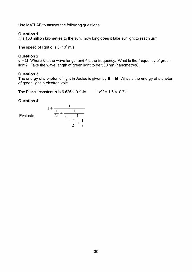
Question 4

Evaluate

1 +1

124

+1

2 +1

124

+18

30

Built-in Functions

Try the following

Just like your calculator, there are functions that you can use in your calculations. Below is a list of some of the more commonly used functions.

abs(x) The absolute value. Modulus ∣x∣

sqrt(x) The square root. √ x

exp(x) The exponential base e. e x

log(x) The natural logarithm. loge(x)

log10(x) The log base 10. log10( x)

round(x) Round to the nearest integer.

ceil(x) Round up.

floor(x) Round down.

fix(x) Round towards zero.

rem(x,b) Remainder of x divided by b.

31

>> pi>> x = cos(pi)>> sqrt(3^2 + 4^2)>> exp(2*log(3) + 3*log(2))

There are two versions of trigonometric functions. There are those that use radians.

The functions that use degrees have an extra d appended to the end of their name.

sin(x) Sine x in radians.

sind(x) Sine x in degrees.

asin(x) The arcsine. The inverse of sin(x). Radians

asind(x) The arcsine. Degrees

sinh(x) Hyperbolic Sine.

asinh(x) The inverse Hyperbolic Sine.

The above variations are also available for the following functions.

cos(x) Cosine

tan(x) Tangent

cot(x) Cotangent

sec(x) Secant

csc(x) Cosecant

Question 5Check that cosh2

( x)−sinh2( x)=1 ?

When x = -1 , x = 0 and x = 1.Why does it not work when x = 20 ? Is the identity wrong or is MATLAB wrong?Hint: Have a look at cosh2

(20) and sinh2(20)

32

>> x = pi/6>> sin(x)>> y = cos(x)>> acos(y)

>> x = 30>> sind(x)>> y = cosd(x)>> acosd(y)

Pass By Value

Lets look in a bit more detail about what happens when you call a function.As an example, we are going to use the square root function. Type the following into the command window.

What happens is this :-• The expression in the brackets is evaluated.• The value of the expression is then passed to the function input.• The function returns the square root of the input.• The output of the function is written into the variable y.

This is called pass by value, because the sqrt function does not know anything about the variables x or y. It only sees the value 49 on the input and it returns the value 7.

Because MATLAB uses pass by value, we can put any expression we like inside the brackets.

Because we just get a value back from the function, we can use the function anywhere in another expression, where you would use a value.

33

Evaluate theexpression

in the bracketssqrt y49 7x

>> x = 49>> y = sqrt(x)

>> y = sqrt(36) >> y = sqrt(5^2)>> y = sqrt(sind(30))

>> sqrt(36) >> 9* sqrt(36)>> log(9*sqrt(36))

Getting Help There are literally thousands of functions available within MATLAB. You are never going toremember all of what is available or how to use them. However, you do not need know all of them. To be a competent MATLAB programmer, you only need to know a small subset of all the functions available. The functions that are used most often.

There will always be a huge number of commands and functions that you do not know anything about. Within this vast collection of commands and functions there could very well be something that does exactly what it is you want to do. As a MATLAB programmer, you will not know all the functions, but you should be able to find out which functions and commands are available and learn how to use them, when you need to. Fortunately, thereare many ways to explore what is available within MATLAB and learn how to use what youfind.

The Function BrowserClick on the fx to the left of the prompt in the command window.

This is the function browser. This allows you to find a function and its documentation and to enter the function into the command window. Try

MATLAB►Mathematics►Elementary Math►Trigonometry

Move the pointer over the functions and wait for the help to appear. Double click on a function to insert at the prompt.

Also have a look at MATLAB►Mathematics►Elementary Math►Exponents and Logarithms

34

The Help CommandYou can get help from the command prompt by typing help followed by the command name. For example, try the following

Later you will be learn how to get help to work with your own programs.

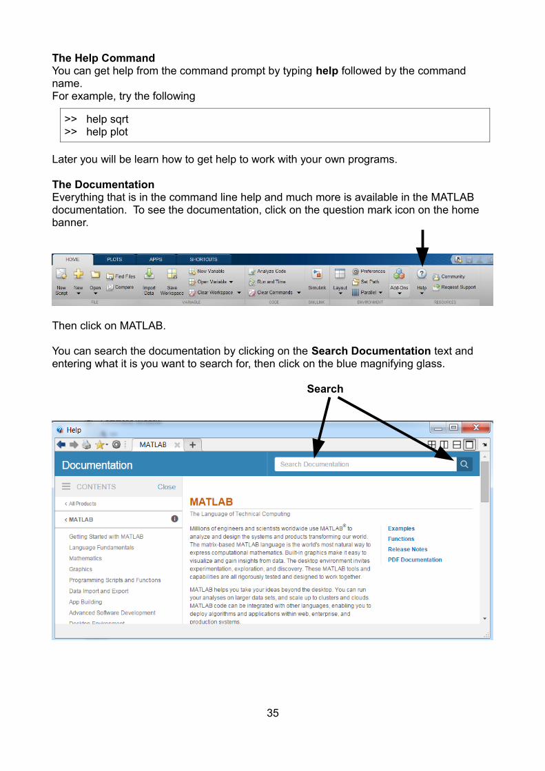
The DocumentationEverything that is in the command line help and much more is available in the MATLAB documentation. To see the documentation, click on the question mark icon on the home banner.

Then click on MATLAB.

You can search the documentation by clicking on the Search Documentation text and entering what it is you want to search for, then click on the blue magnifying glass.

Search

35

>> help sqrt>> help plot

Try searching for logarithm. Until you are a competent MATLAB user, I recommend going to the Refine by Product box on the left and refining your searches to just MATLAB. This cuts out all the help for the various additional toolboxes we have. For the time being you will find more than enough items just in the MATLAB help.

Find the entry for log10 and click on it. Have a look at the help so you have some idea of the style and format of the documentation pages. In particular, note that there are examples. At the end, under See Also, there are links to similar functions. Click on the link to the documentation on the log function and find the difference between the two functions.

Now click on CONTENTS a few times to see what it does.

With the contents visible, click on MATLAB.

Have a look at Getting Started with MATLAB. Here you will find tutorials and videos.

Click on MATLAB again, and then click on Examples on the right. There are lots of examples.

Click on Basic Matrix Operations. Have a quick look.

Return to the help window and click on MATLAB again, and then click on Functions on the right. Try scrolling through the functions available and click on the categories on the left.

Close down the help window and return to the command window. If you need to read the documentation on a particular function, you can open the documentation directly from the command window. Try this

Find the MATLAB functions to answer the following question.

Question 6If you divided 576 by 37, what is the remainder?

Question 7What are the prime factors of 995?

36

>> doc floor

Complex Numbers A complex number is a number of the form

z=a+ib Where i = √ −1

a is the real part of z and b is the imaginary part of z.

A real number can be represented by a point on aline. A complex numbers can be represented by avector on an Argand diagram.

z = r (cosθ+i sinθ )is the polar form of a complex number.

z = r eiθ Is the exponential form.

There are many applications of complex numbers in Engineering, particularly in Electronics and Control. The letter i is used in Electronics to represent an electric current, so Electronic Engineers write complex numbers with a j instead of an i.

z=a+ jb Where j = √ −1

In MATLAB, a variable can be real or complex. You can use an i or a j for the imaginary part. Complex arithmetic is carried out with the normal arithmetic operators. MATLAB automatically detects if a calculation contains complex numbers and carries out the appropriate calculation. Avoid using i and j for non-complex variables.Try the following.

Complex numbers can be entered in either Cartesian, polar or exponential form. Try

37

>> z = 2 + 4j>> w = 5 *(cos(pi/6) + j*sin(pi/6))>> w = 5 * exp(j * pi/6)

>> a = 1 + 2j>> b = 3 + j>> a + b>> a/b

a

b

Real

Ima

gin

ary

r

θ

Argand Diagram

Now try whos again.

Notice that the variables are of type complex. A complex variable requires 16 bytes of memory, twice the size of a double. Two doubles are used to store a complex number. One for the real part and the other for the imaginary part.

Complex numbers have not just been added to MATLAB, the whole package has been designed to work with complex numbers from the very start. So when a function is added to the MATLAB package, the ability to operate on complex numbers is included, provided that a definition of what the function does with complex numbers can be found.

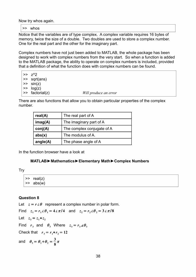
There are also functions that allow you to obtain particular properties of the complex number.

real(A) The real part of A

imag(A) The imaginary part of A

conj(A) The complex conjugate of A

abs(x) The modulus of A.

angle(A) The phase angle of A

In the function browser have a look at

MATLAB►Mathematics►Elementary Math►Complex Numbers

Try

Question 8

Let z = r θ represent a complex number in polar form.

Find z1 = r1θ 1 = 4π /4 and z2 = r2θ 2 = 3π /8

Let z3 = z1∗z2

Find r 3 and θ 3 Where z3 = r3∠θ 3

Check that r 3 = r1∗r2 = 12

and θ 3 = θ 1+θ 2 =38π

38

>> real(z)>> abs(w)

>> z^2>> sqrt(ans)>> sin(z)>> log(z)>> factorial(z) Will produce an error

>> whos

Vectors and Matrices Some of you will not have come across matrices before. There are lectures on matrices and vectors, but perhaps after your first computing laboratory session. So this document includes a brief introduction to matrices sufficient to understand what is going on in the laboratory.

A matrix is a two dimensional array of numbers.

[1 56 7 8.8 7.42

4.6 72 5 92 445 65 77 63 4.23 22 4.11 54 54

]The individual numbers are called the elements of the matrix. When specifying the position of an element or the size of a matrix, the convention is to specify the row before the column. To remember this, I remember R before C like in “Roman Catholic”. The above matrix has 4 rows and 5 columns, so it is a 4 by 5 matrix.

There are ways of adding, subtracting and multiplying matrices together. However, matrix calculations on paper are both limited and tedious. You need to multiply together n3 pairs of numbers to multiply together two n by n matrices. So it is not really practical to multiply very large matrices on paper. To really appreciate matrices, you need a computer.

MATLAB started in the 1970s as a Matrix Laboratory. It was designed to help students do matrix mathematics. Although MATLAB can now be used in many other areas, it is still really easy to do matrix calculations with MATLAB. You can multiply together two large matrices as easily as you can multiply two numbers.

A matrix element can be an integer, a real or a complex number. You do not have to worry about element types. MATLAB will set the element type to what is required.

[1 5 7 8.8 7.42

4.6 72 5i 92 447i 65 77 63 4.2

3+5i 22 4.11 54 5483.2 230 12 41 16

] [12188.817

1.01]

Matrix Column Vector

[12 15 2i −17 3.89 ] 34.2

Row Vector Single Number

Matrices that contain a single row or column are called vectors. In MATLAB, ordinary numbers are regarded as a one by one matrix.

39

MATLAB stores a matrix in an array. Most programming languages use arrays in one formor another. They are a convenient way of handling groups of numbers in a single variable. Unlike matrices, they are not limited to two dimensions. An array in MATLAB can have one, two or more dimensions or be empty. Later in this session, we will look at other operators that are specifically designed to operate on arrays.

Entering Matrices To enter the contents of a matrix :

• Enclose the contents in square brackets.• Separate each element by a space or comma.• Separate each row by a semicolon or new line.

Here are various ways of entering into x a matrix containing [1 2 34 5 67 8 9]

Try whos again.

Notice that the size of the matrix is shown. This can be useful if errors occur.

40

>> whos

>> x = [ 1 2 3; 4 5 6; 7 8 9 ]>>>> x = [ 1, 2, 3

4, 5 67 8 9 ]

>>>> a = [ 1 2 3 ]>> b = [ 4 5 6 ]>> c = [ 7 8 9 ]>> x = [ a ; b ; c ]>>>> x = [ 1 2 3

b ; c ]

When you enter a matrix, you can include other matrices.For Example, try the following :

When adding a row to a matrix, the number of elements in the additional row must be the same as the number of elements in each row of the matrix. The same is true for columns.

Although most of the examples here use numbers, you can use any MATLAB expression to enter a matrix element.

Question 9Add an extra row to D containing 9 and 10.

Question 10

Create a row vector called b containing 22, log10(105) and π

sin−1(1 /2).

Create a new row vector called c, containing a on the left and b on the right.

41

>> x = [ x ; 10, 11, 12 ]>> A = [1 2; 3 4]>> B = [5 6; 7 8]>> C = [ A B]>> D = [ A ; B]

>> a = [ exp(0), sqrt(4) , 1+2 ]

Matrix Operations

Matrix Addition +

These operations treateach of the operands

as a matrix

Matrix Subtraction -

Matrix Multiplication *

Right Matrix Division /

Left Matrix Division \

Raise to a power ^

Transpose matrix ‘

To understand how these work, try the examples below.If you have not done so already, create the two matrices A and B.

>> A = [1 2; 3 4]>> B = [5 6; 7 8] A = [1 2

3 4] B = [5 67 8]

This produces two matrices that we can use in the examples.

>> A + 5 [1 23 4]+5 = [1+5 2+5

3+5 4+5]= [6 78 9]This adds 5 to each element of A.

>> A + B [1 23 4]+[5 6

7 8]= [1+5 2+63+7 4+8]= [ 6 8

10 12]This adds each element of A to the corresponding element in B.

>> A - B [1 23 4]−[5 6

7 8]= [1−5 2−63−7 4−8]= [−4 −4

−4 −4]This subtracts each element of Bfrom the corresponding element in A.

42

>> A * 5 [1 23 4]×5 = [1×5 2×5

3×5 4×5]= [ 5 1015 20]This multiplies each element in A by

5.

>> A'

[1 23 4]

'= [1 3

2 4]Transpose matrix A. Swap rows with columns.

>> M = A * B [1 23 4]×[5 6

7 8]= [1×5+2×7 1×6+2×83×5+4×7 3×6+4×8]= [19 22

43 50]Multiply matrix A by B.

To find the element on the j th row and the k th column of M ( Mjk ) , multiply each of the elements on the j th row of A, by the corresponding element on the k th column of B. Then add all the products together. For this to work, the number of columns of the first matrix must be the same as the number of rows in the second matrix. If the rows and columns do not match, then MATLAB will give you the error Inner matrix dimensions must agree.

Try

In general, A∗B ≠ B∗A Matrix multiplication is not commutative.

>> A ^ 2 [1 23 4]×[1 2

3 4]= [1×1+2×3 1×2+2×43×1+4×3 3×2+4×4]= [ 7 10

15 22]Multiply A by itself

This will only work if the matrix is square matrix. It must have the same number of rows ascolumns.

43

>> B * A

The Identity Matrix

The identity matrix is the matrix equivalent of one.

1× x = x In standard arithmetic

I ×x = x In matrix arithmetic

Where I is the identity matrix.The identity matrix is all zeros, except for a diagonal which is all ones. There is a MATLABfunction for I. It is called eye.

Try your own 2 by 1 matrix.

The Inverse of a Matrix

A ∗ A−1 = I

Where A−1is the inverse of A

The function inv can be used to find the inverse of a matrix.

44

>> eye(5)>> I = eye(2)>> x = [3;4]>> I * x

>> inv(A)>> A^-1>> A * inv(A)>> inv(A) * A

Using Matrices to Solve a Set of Linear Equations

You will all have solved two simultaneous equations in two variables such as the ones below.

x1+2 x2 = 53 x1+4 x2 = 11

You may have also solved three equations in three variables or four equations in four variables, but as the amount of calculations required increases cubically with the number of variables, you will not be expected to solve much larger problems by hand. In the real world of Engineering, there is no such limit on the size of the problem. The only practical way to solve those types of problem is to use a computer. You can use MATLAB to solve large sets of simultaneous equation. To see how you can do this, start by solving the pair of equations above using matrices and MATLAB.

x1+2 x2 = 53 x1+4 x2 = 11

In matrix form this becomes :

[1 23 4][x1

x2]= [ 5

11]Or simply

A x = b Where A= [1 23 4] x = [x1

x2] b= [511]

If you multiply both sides by A−1(the inverse matrix of A ).

A−1 A x = A−1b

I x = A−1b

x = A−1b

Then check that you have the correct solution.

You don't need a computer to solve the above, but when you have much more than two sets of equations, it becomes a lot harder to solve by hand.

45

>> A = [1 2; 3 4]>> b = [5 ; 11]>> x = inv(A)*b

>> A * x

It would be very tedious indeed to attempt to solve the following problem by hand.

2 x1+4 x2+7 x3+9 x4+8 x5 = 1076 x1+9 x2+2 x3+5 x4+2 x5 = 606 x1+3 x2+5 x3+1 x4+8 x5 = 71

x1+5 x2+6 x3+x4+2 x5 = 43x1+2 x2+8 x3+2 x4+9 x5 = 82

However, it is very easy to solve this in MATLAB.

Matrix division is not something that you will find in normal mathematical text books. As you would expect, matrix division is the inverse of matrix multiplication. Try this

This is the equivalent to inv(A) * b, but Matrix division is performed using Gaussian elimination, which is a bit more efficient than finding the inverse of the Matrix.

Because matrix multiplication is not commutative :

inv (A) B ≠ B inv(A)

there are two division operators.

Left Division Right Division

The inverse is to the left The inverse is to the right

A \ B ≡ A-1 B B / A ≡ B A-1

46

>> A = [2 4 7 9 8; 6 9 2 5 2; 6 3 5 1 8; 1 5 6 1 2; 1 2 8 2 9] >> b = [107; 60; 71; 43; 82]>> x = inv(A)*b

>> x = A\b

It is not always possible to find an answer. For example

Let A= [1 −2 3

−2 4 −61 5 9 ] and b = [

1−23 ]

Try to find an x such that A x = b

If A is singular, there is either no solution or an infinite number of solutions.The determinant of a singular matrix is zero.

A singular matrix has no inverse.

Question 11

Find x when [5 9 −41 −9 65 −2 2 ]x = [

−348047 ]

47

>> det(A)

>> inv(A)

>> A = [ 1 -2 3 ; -2 4 -6 ; 1 5 9 ]>> b = [ 1 ; -2 ; 3 ]>> x = A \ b

The Colon : Notation

This is used to generate vectors for graphs and it is also used for loops. You can think of itas an arithmetic series generator. For example.

This statement produces a vector containing [1, 2, 3, 4, 5]. In general

a : b Is a row vector. The first element is a, the last is b.Each element is one larger than the element to its left.

There is a second form where you can specify the spacing between the elements.a : s : b Is a row vector. The first element is a, the last is b.

Each element is s larger than the element to its left.

Try the following examples.

Linspace

The linspace function is an alternative to the colon notation. It creates a row vector with a specified number of points. Suppose that you want a row vector with 5 elements, evenly spaced between zero and 10.

Which is equivalent to x = [0 2.5 5 7.5 10]

In general, if you want a specific number of elements, linspace is easier to use. If you wanta specific spacing then the colon notation is easier to use.

An example of using linspace to plot a pentagon.

Try plotting a hexagon.

48

>> k = 1:5

>> k = 1:10>> v = 0:5:20>> w = 0:0.25:1>> y = -pi:pi/5:pi>> z = 6:-1:1

x = linspace(0,10,5) x = linspace(0,10,5) >> x = linspace(0,10,5)

>> n = 6>> t = linspace(0,2*pi,n)>> x = cos(t)>> y = sin(t)>> plot(x,y)

Array Operators Very often you need to perform the same mathematical procedure on lots of different numbers. Suppose that you want to plot a function. You need to evaluate the function for many different values so that the points can be plotted onto a graph.

For example, to plot y = x 2

You can use the colon notation to generate a vector containing all the values of x.

The raise to a power operator (^) by default tries to square a matrix, which will not work on a vector. Try it.

We cannot use the matrix operator because x is not a square matrix. However, we do not want to square a matrix, we want to square each of the individual elements. That is just what the array operator does.

The operator symbol has two characters ( .^ ). To distinguish the array operator from the matrix operator, each of the array operators has a dot at the front.

Look at y and make sure that it is what you expect. Now we can plot the graph.

You can get a much better graph if you use a smaller step size. Do that now.

49

>> x = -5 : 5

>> y = x^2

>> y = x .^ 2

>> plot(x,y)

Array operations act on corresponding pairs of elements in each of the operands. They are some times called Element by Element Operators or Element-Wise Operators.

Array Multiplication .*Right Array Division ./Left Array Division .\Raise to a power .^

The operands must be the same size, unless one of the operands is a single number. Enter the following examples and compare with the examples of matrix operations.

You will probably have to recreate the two matrices A and B.

>> A = [1 2; 3 4]>> B = [5 6; 7 8]

A = [1 23 4] B = [5 6

7 8]>> A .* B [1 2

3 4] .∗[5 67 8]= [1×5 2×6

3×7 4×8]= [ 5 1221 32]Multiply each element in A

by the corresponding element in B.

>> A ./ B [1 23 4] . /[5 6

7 8]= [1 /5 2 /63 /7 4 /8]= [ 0.2 0.3333

0.4286 0.5 ]Divide each element in A by the corresponding element in B.Array operations are commutative. Therefore A./B = B.\A

>> A .^ 2

[1 23 4] .∧ 2 = [12 22

32 42]= [1 49 16]Square each element in A

>> A .^ B

[1 23 4] .∧[5 6

7 8]= [15 26

37 48]= [ 1 642187 65536]Raise each of the elements in A

to the power of the corresponding element in B.

To remember which operators are which, think of MATLAB as the Matrix Laboratory. Therefore the default action is for the operators to do matrix arithmetic.

There is no distinction between matrix and array variables. There is only one type of variable that can be used for arrays or matrices.

As you get more experience of using MATLAB, you will find that most of the time you will be using array arithmetic. It is not a bad idea to get into the habit of inserting a dot before all multiplications, divisions and raising to the power operators, unless you know that you want a matrix operation.

50

Question 12Plot y = x3

−13 x + 12 between -5 and 5.

Example

Meshgrid is a function that returns two arrays. The first contains the x coordinates the second the y coordinates.

The variable z contains points of an Argand diagram. Now we can draw 3-D plots of complex functions.

Click on the icon Rotate 3D icon and drag the mesh.

51

>> [x,y] = meshgrid(-5:5)

>> z = x + j*y

>> f = z.^2>> mesh(x,y,abs(f))

Functions of Arrays and MatricesMost functions are designed to work on arrays. If you apply an arithmetic function to a array, then the function is applied to each of the elements in the array.

>> sin(A)sin[1 2

3 4]= [sin (1) sin (2)sin (3) sin (4)]

>> exp(A)exp[1 2

3 4]= [e1 e2

e3 e4]>> sqrt(A)

sqrt[1 23 4]= [√1 √2

√3 √4]These functions are specifically designed to operate on matrices.

>> inv(A) The inverse of A

>> det(A) The determinant of A

>> norm(A) The norm of A

>> [v,d]=eig(A) d = Eigenvalues v = Eigenvectors

>> S = sqrtm(A) Matrix square root

>> S * S

Then there are array generating functions

>> zeros(3) 3 by 3 array of zeros

>> zeros(3,4) 3 by 4 array of zeros

>> zeros(3,4,2) 3 by 4 by 2, 3 dimensional array of zeros

>> ones(3,4) 3 by 4 array of ones

>> rand(3,4) 3 by 4 array of random numbers

>> eye(3) 3 by 3 identity matrix

In the function explorer, look at MATLAB►Mathematics►Linear Algebra

There are a lot of functions here that you will not be able to understand. You will learn about things like Eigenvalues and Eigenvectors in the Mathematics Lectures. A lot of the Mathematics here is outside the scope of the course.

Question 13Plot the function f (x )= sin( x) between 0o and 360o.

52

Accessing Elements in a Matrix (Indexing)Supposing you have a row vector.

In mathematics you use an index to refer to a particular element of the vector. The third element would be a3, where 3 is the index. To do the same in MATLAB, you place the index in round brackets after the name of the variable.

In MATLAB, indexing starts at one. So the first element is a(1), the second a(2) etc.You can use indexing in any MATLAB expression.

If you put a vector of index values in the brackets, you can obtain a new vector with just the specified elements. Try the following.

>> a([3,5]) [10 11 12 13 14 15]

>> a(3:5) [10 11 12 13 14 15]

>> a(3:end) [10 11 12 13 14 15]

You can also replace specified elements within the original vector.

>> a(3) = 5 a = [10 11 5 13 14 15]

>> a(3:5) = 7 a = [10 11 7 7 7 15]

>> a(3:5) = [9 4 2] a = [10 11 9 4 2 15]

Question 14

(a) Display the 2nd to 6th elements of a.

(b) Display the 2nd and 6th elements of a.

(c) Set the 6th element equal to the 1st element.

53

>> a = 10:15

>> a(3)

If you want to index into a matrix, we simply add another index, the first specifies the row and the second the column.

>> M = [1 2 3 4 5 6 7 8 9 10 11 12]

M = [1 2 3 45 6 7 89 10 11 12]

>> M(2,3) [1 2 3 45 6 7 89 10 11 12]

>> M(2,[1 2 4]) [1 2 3 45 6 7 89 10 11 12]

>> M(2,2:4) [1 2 3 45 6 7 89 10 11 12]

>> M([1 2],3) [1 2 3 45 6 7 89 10 11 12]

>> M(:,3) [1 2 3 45 6 7 8

9 10 11 12]A single colon is used to specify all rows. A single colon in the column section specifies all columns.

>> M(1,:) [1 2 3 45 6 7 89 10 11 12]

>> M(2,3)=99 M = [1 2 3 45 6 99 89 10 11 12]

>> M(1:2,3)=0 M = [1 2 0 45 6 0 89 10 11 12]

>> M(1:2,[3 4])= [21 22;23 24] M = [1 2 21 225 6 23 249 10 11 12]

>> M(3,:)= M(3,4:-1:1) M = [1 2 21 225 6 23 2412 11 10 9 ]

54

Question 15

(a) Display the 2nd to 4th elements on row 1 of M.

(b) Display the 2nd and 4th elements on row 1 of M.

(c) Display the 2nd and 4th elements on row 1 and row 3 of M.

(d) Display the 2nd and 4th columns.

(c) set M14 to M34 + 5.

Question 16

Use the meshgrid function to generate two matrices x and y.

Using the appropriate operator, multiply x and y to get an infant school type multiplication table.

Use indexing to find 5 x 7 from the table.

Display the 7 times table by using indexing to display the 1st and 7th row of the table.

55

>> [x,y] = meshgrid(1:12)

Scripts Typing commands at the MATLAB prompt is bearable for small sets of operations and for checking how a command works. However it is hopeless for carrying out anything more elaborate. Supposing that you are doing something that requires many MATLAB commands. If you make a mistake or want to change something, you may have to enter every command again. It does not take very long for this to become tedious. The solutionis to put all the commands required into a file. A script is a text file containing a list of MATLAB commands. Essentially it is a Matlab program. When you ask MATLAB to run the script, it starts at the top of the file and carries out each of the commands, one after theother, in sequence. The file will have a name something like myscript.m, with an .m file name extension to show that it is a MATLAB file.

You can use any text editor such as gedit to write a script, but Matlab has its own editor which makes it very much easier to write, and check for errors.

Using the Matlab editor

1. Type edit at the Matlab's command prompt to start the MATLAB editor.

2. Type the code below into the editor.

3. Save the file as mygraph.m by selecting Save on the left side of the banner at the top of MATLAB, then selecting Save As...

4. At the command prompt type

Matlab will seek out the file called mygraph.m and execute each of the commands within the file one at a time starting at the top. Any command that you have used in the command window can be used in a script.

56

>> mygraph

%plot a cosine wave

x = linspace(0,2*pi,100); %100 points between 0 and 2 pi y = cos(x); plot(x,y)

>> edit

Comments

The percent sign %, is used to indicate a comment.

Any text after the percent sign is ignored by MATLAB. In all branches of Engineering, documentation is required so that you can inform other people what and why you have done something. Programmers use comments in their programs to add extra explanation to make the program understandable. For the short three line script we have just entered itis hardly needed, but as your programs get longer and more complex, it will become essential.

At the beginning of any program, you should state what the program is for and how to use it. In MATLAB, this first block of comments is particularly significant, as it is the helpfor the program.

57

%plot a cosine wave

>> help mygraph

Basic 2D Plotting We are going to use the script mygraph created earlier to explore the various ways of plotting graphs. First add a second plot command at the end of the script.

Click on the green arrow on the icon banner ofthe editor to save and run the script.

At the moment, the first graph is immediately overwritten by the second. So you cannot see the first graph. We can plot the second graph in another window. The window that contains the image of the graph is called a figure. The figure command creates a second figure. In the script, between the two plot commands, enter :

You will have to drag the top figure to one side to see the figure underneath.

We can also plot both graphs separately in the same figure. Delete the figure command that you entered above. Above the first plot enter

and above the second plot add :

And see what effect it has. Try changing the arguments so that you get one row and two columns.

You can also plot both functions onto the same graph. Delete the two subplot commands and place

between the two plots. This holds the plot on the graph while the new graph is plotted over the top.

58

y1 = sin(x); plot(x,y1)

figure

subplot(2,1,1); % Two rows, one column, first graph

subplot(2,1,2); % Two rows, one column, second graph

hold on

The problem is now that as both graphs are the same colour, it is difficult to distinguish them. So next, specify the colour of each of the plots. Change the first plot to

and the second to

This plots the cosine wave in red and the sin wave in green.

The tables below show different ways of using the plot function.

plot(y) Plot y against index number.

plot(x,y) Plot y against x

plot(x1,y1,x2,y2) Plot y1 against x1 and y2 against x2.

plot(x,y,'r+') Plot y against x using red plus signs.

plot(x1,y1,'r+',x2,y2,'go') Red plus signs for x1 and y1, Green circles for x2 and y2.

There is much more information about plot in the online documents.

There are lots of different line styles and colours that you can use.

Symbol Line Type or Mark Symbol Colour

. Point r Red

o Circle g Green

x X mark b Blue

+ Plus sign y Yellow

* Stars m Magenta

- Solid line c Cyan

: Dotted line w White

-. Dash dot line k Black

-- Dash Line

This is not the complete list of what is available. Look at the MATLAB documentation, to see all the symbols you can use.

59

plot(x,y1,'g')

plot(x,y,'r')

doc lineSpec

doc plot

There are many different types of graphs.

Other Types of Plot

fill(x,y,'r') Red filled graph

bar(x,y) Bar graph

stem(x,y) Stem plot

loglog(x,y) x & y log scale

semilogx(x,y) x log, y linear

semilogy(x,y) x linear, y log

polar(theta,r) Polar plot

surf(x,y,z) 3D surface

mesh(x,y,z) 3D mesh

plot3(x,y,z) 3D line plot

Example

Example

The first definition used for the constant e is e = limn →∞

(1+ 1n)

n

This example explores how fast this converges.

60

% Convergence of Euler's definition of e k = 0:19; n = 2.^k; % n starts at 1 and stops at 524288 e = ( 1 + 1./n).^n; % approximation of e semilogx(n,e,'rx') grid

% Calculate the number of operations required to solve n equations % using Gaussian Elimination n = 1:12; % Number of equations op = n.*(4.*n.^2 + 9.*n - 7)./6; % Number of operations required bar(n,op);

Other Graphics Commands

Matlab will automatically scale the graph, but sometimes this is not what you want. Returning to the script mygraph and look at the graph displayed. You will notice a gap on the right hand side where MATLAB has scaled the graph to the nearest whole unit. So nowwe are going to change the limits of the graph so that there is no gap. At the bottom of thescript, add the following:-

The axis command takes one four element vector as an argument. [minX maxX minY maxY]In this case the range of the x axis is from zero to 2π, and the y axis is from -1.1 to 1.1

Title and label the graph by adding the following to the end of the script.

Add a grid

and add a legend

You can drag the legend about the graph. Your graph should now look like this.

61

xlabel('Angle (rads)'); ylabel('Value'); title('My Graph');

grid on

legend('cos(x)','sin(x)');

axis([0 2*pi -1.1 1.1]);

The following table is in the MATLAB quick reference

Other Graphics Commands

title('Title') Graph title.

xlabel('X axis') Label the x-axis.

ylabel('Y axis') zlabel('Z axis')

Label y and z axis.

text(x,y,'My Text') Place text at coordinates x,y.

grid Place a grid on the graph.

hold on Add any new plot to the current graph.

hold off Replace current plot with any new plot.

subplot(r,c,n) Split figure into r rows by c columns of subplots.

subplot(2,3,1) subplot(2,3,2) subplot(2,3,3)

subplot(2,3,4) subplot(2,3,5) subplot(2,3,6)

axis([minX maxX minY maxY]) Set the limits of the graph in X and Y.

h = figure New graphics window.

figure(h) Change to plotting in figure h.

delete(h) Delete figure h.

clf Clear current figure.

drawnow Force the graph to update now.

62

End of Session ExercisesWork through the following questions. These exercises are a part of the assessment for this session. You will need to show a demonstrator how you answered the questions. For each question, put the solution into its own script. Suggested script names are q1.m q2.m etc.

File management is part of the assessment. All files produced must be in a directory designated for this set of exercises and only for these exercises. The recommended location for these exercises is P5computing/Session1/Exercises.

Exercise 1

Find w, x, y and z when

2 w+3 x+7 y+ z = 21w+0.5 x+y+2 z = 113 w+x+y−3 z =−8−w+x+3 y+z = 10

Check that the answer is correct.

Exercise 2(a) Set the variable a to all the integers from 1 to 5.

(b) Set b to a + 10

(c) Form a new 2 by 5 matrix called c, with a on the top row and b underneath.

(d) Form a new 2 by 10 matrix called d, with c on the left and c + 5 on the right.

(e) Form a 10 by 10 matrix called M. The top two rows of M will be d. Below that will be d + 20 and below that will be d + 40, then d + 60, then finally d + 80.

(f) Set x to the 4th element on the 9th row of M.

(g) Set y to M3,7

(h) Set z to the 5th column of M.

(i) Set Me to the even numbered columns of M and Mo to the odd columns.Me should contain all the even numbers and Mo the odd numbers.

(j) Multiply Me by Mo using array multiplication.

(k) Multiply Me by the transpose of Mo using matrix multiplication.

63

Exercise 3

Plot a graph of y = x3−2 x2−x+2 between x =−3 and x = 3 .

Exercise 4Jν (z) is the Bessel function of first kind of order ν , where ν is the Greek letter nu.Plot J1 (z), a Bessel function of the first kind of order one, between 0 and 20.

This exercise tests your ability to use the MATLAB help. Find the MATLAB function for theBessel function of the first kind and how to use it and plot the graph, just like you would plot sin(x).

• It must be a MATLAB function that you use, not a symbolic math toolbox function or a function from any other toolbox.

• There are several different types of Bessel function, make sure you find the correct one. A modified Bessel function is something different.

Exercise 5Write a script that calls the scripts that your wrote for the previous two exercises, so that both graphs are displayed in the same figure. The graph for exercise 3 should be in the top half of the figure with the graph for exercise 4 in the lower half.Give each graph a title and a grid.

64

Exercise 6The Trapezoidal Rule is a method of performing numerical integration. The integral of a function is equal to the area under the curve. We can split the area under the curve of a function into a series of strips, each h wide.

We can approximate each strip by a trapezium. By finding the area of each trapezium, we can find the approximate area under the curve.

∫x1

x n

f ( x)dx ≈f 1+ f n

2h + h ∑

k = 2

n−1

f k

Using the trapezoidal rule to find

y =∫0

13 x2

+1 dx with h = 0.1

Hint: Use subscripting to find f1, fn and [ f2, f3, - - - , fn-1]Find out what the sum function does.

On paper, calculate the actual value of y.At the bottom of the script calculate the error.

Change h to 0.01 and see what happens to the error.

Note

∑k = 2

n−1

f k = f 2 + f 3 + f 4 +⋯+ f n−1

65

x1 x2 x3 xn x

f k = f (xk)h

f 2

f 1

f 3 f n

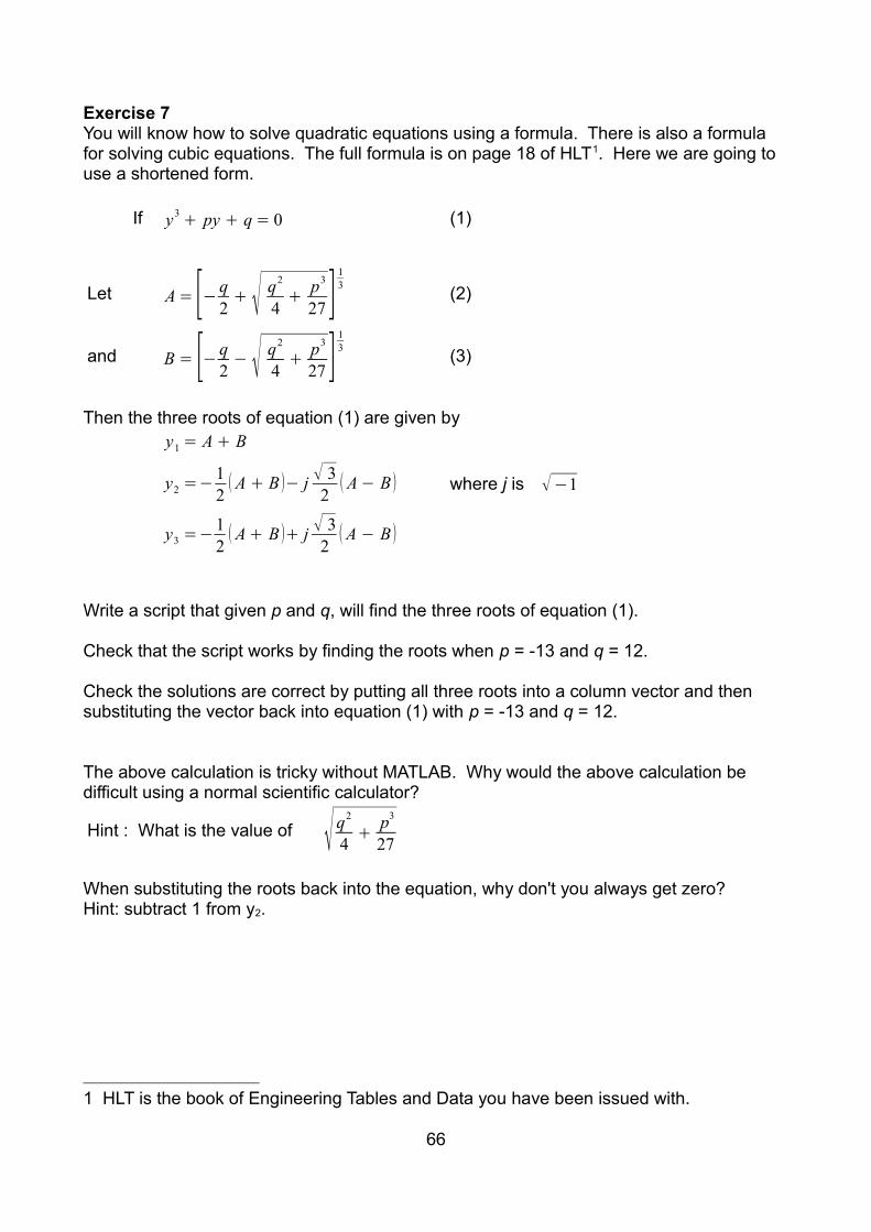
Exercise 7You will know how to solve quadratic equations using a formula. There is also a formula for solving cubic equations. The full formula is on page 18 of HLT1. Here we are going to use a shortened form.

If y3+ py + q = 0 (1)

Let A = [− q2

+ √ q2

4+

p3

27 ]13

(2)

and B = [− q2

− √ q2

4+

p3

27 ]13

(3)

Then the three roots of equation (1) are given byy1 = A + B

y2 =−12

( A + B )− j √ 32

( A − B ) where j is √−1

y3 =−12

( A + B )+ j √ 32

( A − B )

Write a script that given p and q, will find the three roots of equation (1).

Check that the script works by finding the roots when p = -13 and q = 12.

Check the solutions are correct by putting all three roots into a column vector and then substituting the vector back into equation (1) with p = -13 and q = 12.

The above calculation is tricky without MATLAB. Why would the above calculation be difficult using a normal scientific calculator?

Hint : What is the value of √ q2

4+

p3

27

When substituting the roots back into the equation, why don't you always get zero?Hint: subtract 1 from y2.

1 HLT is the book of Engineering Tables and Data you have been issued with.

66

Exercise 8 In this exercise, you will process data from an experiment. The data is from a tensometer. A tensometer is a device for testing the strength of a specimen. The specimen is slowly stretched and the applied load and the displacement (the amount the specimen has been stretched) are both recorded. You will be using a tensometer in the Mechanical Laboratory.

In a terminal window copy the file.

Assuming that you are working in ~/P5computing/Session1/Exercises.Open the file with gedit. You will see that on each line there are two numbers. The first number is the Displacement in mm. The second number is the applied load in kilonewtons. This is a comma separated variable file (csv).

In MATLAB enter

The load function has copied the whole of the file contents into the array, TestData.

(a) Write a script that will • Load in the test data from the file. • Separate the displacement and the load.• Plot the load against displacement.• Label the axes, add a title and a grid.

(b) Try the following in the command window.

Look up the function max in the MATLAB documentation to find out what M and I are.

(c) Use the max function to find the coordinates of the point on the graph where the loadis maximum.

(d) Plot the point on the graph where the load is maximum using a red cross.

(e) Use the text function to write “maximum load” next to the red cross.

67

cd ~/P5computing/Session1/Exercisescp /Documentation/P5comp/TestData.csv .

>> load TestData.csv>> whos TestData

>> A = [ 1 2 6 4 7 5 2]>> max(A)>> [M,I] = max(A)

Exercise 9Write a script that will plot the four coordinates (-1,4), (0,2), (1,0), (2,4) as red crosses.Hint : Collect the x and y coordinates and plot a single graph.

Use the function polyfit to find the coefficients of a cubic equation that goes through all fourpoints. Then use polyval to plot the cubic equation between x = -3 and x = 3, in green, over the top of the four red points in the same graph. The green line should go through the centre of each cross.

Assessment When you have finished ask a demonstrator to assess your work. The demonstrator will want to see the results of the exercises.

If you finish early, start on the next session. It will be to your benefit to make an early start on session 2.

68

Practice 1There is now a four week gap before Session 2. This is more than sufficient time for you to forget everything you have learned about MATLAB in the first session. This will make Session 2 difficult. So between now and session 2, you need to consolidate what you have learned in Session 1. The best way of doing this is to start using MATLAB.

• If you have not done so already, install MATLAB onto your own computer. Download the installation instructions from :-https://register.oucs.ox.ac.uk/self/software

• If you do not have a computer, you can use a computer in Software Laboratory A, B or the Design Office. Even when a scheduled laboratory is running, there are nearly always spare computers for you to use.

• If you do have your own computer, try accessing your home area on the Departmental file server on your own computer. There are instructions on doing this on the Departmental web site.http://www.eng.ox.ac.uk/ecsg/machines/undergraduate-it-support

The more you use MATLAB, the easier it becomes. There are several things you can do between now and the next session.

• Play with MATLAB. You cannot do any damage by just messing around with MATLAB. Challenge yourself. Try writing your own programs. Have fun.

• Use MATLAB for other course activities. It is not cheating to check your answers are correct by using MATLAB.

• Try out the activity on the next page.

69

Practice ActivityThis activity will allow you to get more practise using MATLAB. It will also introduce you tosome of the things that you will learning about in session 2. Don't take it too seriously. I hope that you will enjoy this activity and have some fun doing it.

Imagine a disc of radius b, rolling around the inside ofa circle of radius a. On the disc there is a point p thatis a distance r from the centre of the disk. The track ofthe point p as the disk rolls around inside the circle isa hypotrochoid. By varying a,b and r, you obtain ahuge variety of different patterns.

This activity is about plotting hypotrochoids. You willlearn how to combine several hypotrochoids to form apattern. You will also learn how to do animation.

Plotting a hypotrochoid

Write a script to plot a hypotrochoid. The coordinates of the point p can be found using the following formula.

x =(a + b)cosϕ − r cos( a + bb

ϕ )y = (a + b)sinϕ − r sin( a + b

bϕ )

Where ϕ is the angular distance that the disc has moved.

Write a script that plots a hypotrochoid.• To start with set a to one, b to -1/5 and r to 1/5.

• You will need over a hundred values of ϕ between zero and 2π.

• Evaluate x and y for all the different values of ϕ.

• Plot y against x.

• Add the command axis equal after the plot. This gives the axes an equal scaling, otherwise the plot will be distorted.

If b is positive, you get a different shape called a epitrochoid. This is what you get if you roll the disc on the outside of the circle.

70

a

b

rp

Unfortunately, the script as it is at the moment will not work for all hypotrochoids. Sometimes, the disc has to go completely around the circle several times for the curve to join up. Try changing b to -2/5.

The disc needs to go around twice, so change ϕ so there are two hundred points between zero and 4π. Then run the script.

Now change b to -3/5, and rerun the script.

This time, the disc needs to go around three times, so change ϕ so there are three hundred points between zero and 6π.

I hope that you can see that it is the numerator of the fraction that determines how many times the disc needs to go around. So do the following :-

• Set b to – p/q.

• Set the number of points n to 100 x p.

• Change ϕ so that it goes between zero and 2πp.

• Set p to 4 and q to 5

Now play around with the values of p, q and r and see what different patterns you get.

A hypotrochoid function

The next objective is to produce a plot with lots of different hypotrochoids. To make it easier to do this, we are going to turn the script into a function.

• Save the script you produced for the above as hypotrochoid.m

• Insert the following at the very top of hypotrochoid.m

This turns the script into a function.

• Remove any assignments of p,q and r from the script.

To check that the function works, enter the following into the command window.

This should plot a hypotrochoid with p set to 1, q to 3 and r to 0.3.

Try testing with your own values of p,q and r.

71

function hypotrochoid(p,q,r)

>> hypotrochoid(1,3,0.3)

For Loop

What does r do to the shape of the hypotrochoid?To find out, we can use a for loop to plot several hypotrochoids, with different values of r.Enter the following into a script.

This is a 'for loop'. The two lines between the for and the end are said to be within the for loop. They are repeated 5 times, once for each value in the vector 0.1:0.1:0.5.The value of r is different for each loop, taking each value in the vector in turn. So for the first time around the loop, r =0.1, then 0.2, then 0.3 etc.

Animation

Sometimes it is easier to see what is happening when the graphs are one after the other, instead of on top of each other.

Save the previous script to a new file and change it to the following.

• The number of graphs plotted has been increased from 5 to 200. A 5 frame animation is too brief.

• Try commenting out the axis command (put a % at the start of the line). Then you can see what happens if you allow the graph to autoscale. You many need to increase the size of the graph for different hypotrochoids.

• Uncomment the axis command and comment out the drawnow and the pause. Without the drawnow, you only see the very last graph. The pause command is useful for slowing down the animation.

Set p to 1, instead of 3 and see what effect it has.

72

% Plot many hypotrochoids with different values of r for r = 0.1:0.1:0.5 % for each value in [0.1,0.2,0.3,0.4,0.5] hypotrochoid(3,4,r) % Plot a hypotrochoid with the next r hold on % We want to see all the hypotrochoidsend legend('0.1','0.2','0.3','0.4','0.5')

% Plot many hypotrochoids with different values of r for r = 0.01:0.01:2 hypotrochoid(3,4,r) % Plot a hypotrochoid with the next r axis([-2 2 -2 2] ) % Keep the same scale for each plot drawnow % Force the graph to display now pause(0.05) % A delay, in secondsend

Now try p = 1 and q = 57. Although the pattern produced is interesting, this is not a hypotrochoid. The graphs do not have a sufficient number of points to show the plot in detail. Hence, there are lots of straight lines.

Edit the function hypotrochoid.m and change the number of points plotted to 1000 x p, instead of 100 x p. Save the function and run the script again.

You will notice that even with 1000 points per revolution, you can still see the straight sections on some of the curves. In general, you need more points for higher values of q. On the other hand, if it is interesting patterns you want, you may want to experiment with fewer points.

Orientation

Now we are going to change the function so that you can rotate the hypotrochoid. • Edit hypotrochoid.m and change the formula for x and y to add an extra angle t.

x =(a + b)cos(ϕ+t )− r cos(a + bb

ϕ)y = (a + b)sin (ϕ+t )− r sin(a + b

bϕ)

• Change the function definition at the top of the file to include angle t.

Save the previous script to a new file and change to the following.

73

function hypotrochoid(p,q,r,t)

% Plot many hypotrochoids with different values of angle t for t = linspace(0,2*pi,200); hypotrochoid(3,4,1,t) % Plot a hypotrochoid with the next t axis([-2 2 -2 2] ) % Keep the same scale for each plot drawnow % We want to see all the hypotrochoids pause(0.05) % A delay, in secondsend

Location

You can also change the location of the hypotrochoid. • Edit hypotrochoid.m and change the plot line to :

• Change the function definition at the top of the file to include the location.

Then test the new function with the following script.

The problem with using linspace directly for the vector of a for loop, is that you can only change one quantity at a time. In the example below, several different quantities are changed on every loop. The loop variable k is the index of the vectors. Within the for loop, the index is used to look up the value of each quantity, in the relevant vector.

74

function hypotrochoid(p,q,r,t,x0,y0)

% Plot many hypotrochoids at different locations for L = linspace(0,10,6) hypotrochoid(3,4,1,0,L,L) % plot a hypotrochoid at the next location hold on % We want to see all the hypotrochoidsend

plot(x+x0,y+y0)

% Plot many different hypotrochoids in a spiral n = 50; %The number of hypotrochoids to plot. R = linspace(2,1,n); % The radius of the circle.theta = linspace(0,3*pi/2,n); % The angular position of the hypotrochoidX = R .* cos(theta); % The x coordinates Y = R .* sin(theta); % The y coordinatesT = linspace(0,2*pi,n); % orientations for each hypotrochoidRh = linspace(0.01,1,n); % the values of little r for k = 1:n t = T(k); r = Rh(k); x=X(k); y=Y(k); hypotrochoid(1,4,r,t,x,y) % Plot the next hypotrochoid axis([-3 3 -3 3]) % Keep the same scale for each plot drawnow % We want to see all the hypotrochoids pause(0.1) % A delay, in seconds hold onend

Now it is up to you

• You now have a function that can plot different hypotrochoids at various locations and orientations.

• You know how to plot many hypotrochoids with different properties using a for loop.

• You know how to animate hypotrochoids.

Have a go at writing your own programs to make your own patterns and animations.

If you would like to get even more practice, have a look at :-

www.eng.ox.ac.uk/~labejp/Courses/1P5/Practise1Extra.pdf

75

76

Session 2

Programming In this session you are going to learn much more about programming. You will learn aboutloops, conditional statements and functions. Although you will be using MATLAB, all of these programming features are also found in most programming languages.

You are going to create many MATLAB programs. Before you start, create a new directory (folder) to store these programs. You can do this within the MATLAB Command Window.

cd P5computingmkdir Session2 cd Session2

Or you can use the far left hand window in MATLABwhich is just like a file browser, or Windows explorer.

By now you should realize that you are expected to keepyour file system neat and tidy. At the end of the day, weexpect your P5computing directory structure to looksomething like the diagram on the right.

Work through the notes as you did in session 1. Remember, if you see a box like this :-

it means enter commands at the MATLAB prompt >>, in the command window.

If the box does not contain a MATLAB prompt

then this should be entered into a MATLAB program using the MATLAB editor.

77

>> a = 'P'>> whos

for k = [1,-2,47,4] fprintf('k = %d \n',k);end

abc0123

P5compting

Session1 Session2

Your Home Directory

Exercises Exercises

Character and String Variables

In addition to manipulating numbers, many programming languages allow you to manipulate text. Variables of type char hold a single text character.

What is actually stored in a is the number 80, the ASCII1 character code of the letter P. Tosee this, there is a function for converting data to type double.

There is also a function to convert data into a char.

88 is the ASCII code for the letter X.

Strings

A string variable is used to hold a piece of text.

A string is the equivalent of a one row array of chars.

This means that you can use indexing on a string.

You can join several strings together.

1 ASCII is the American Standard Code for Information Interchange. It is a standard code for representing text on digital devices.

78

>> a = 'P'>> whos

>> double(a)

>> c = char(88)

>> T = 'P5 Computing'

>> S = [ 'A' 'B' 'C' ] >> whos T S

>> T(4)>> T(4:7)

>> W1 = 'Engineering'>> W2 = 'Science'>> space = ' '>> W = [ W1 space W2 ]

You can display text in the command window,

or in a message box,

or on a graph.

Where (0.2,0.6) are the (x,y) coordinates of the text on the graph.

Formatted Output

The fprintf function is used to provide “formatted output” rather than the untidy output one gets from the prompt. In its simplest form, it will just print out a line of text. Try the following:- Remember that you can use the up arrow key to recall and edit previous commands.

The \n inserts a new line. You can also use \t to insert a tab.

You can also include the value of a variable in the text.

79

>> fprintf ('Hello World' )>> fprintf ('Hello\n World\n' )

>> fprintf ('Hello\t World\n' )

>> x=pi>> fprintf ('x = %f\n',x )

>> disp(W)

>> msgbox(W)>> msgbox(W,'My Title')

>> title(W)>> text(0.2,0.6,T)

For each variable whose value you wish to print, there must be a matching field in the formatting string starting with %. The %s is for a string, the %d prints an integer, and %f prints a fixed point number. Try

You can also specify the number of decimal places you want.

fprintf Formats %d Integer %5f 5 characters wide \n New line

%f Fixed point %5.2f 2 decimal places \t Horizontal tab

%e Exponential Notation %-5.2f Left justify \\ Back slash

%s String of Characters %+5.2f Print sign (+ or -) %% Percent character

For more information, see

You can form a string that contains numerical values by using sprintf function. This is almost identical to the printf function, except that the output is a string.

80

>> x = 42>> str = sprintf( 'The value of x is %d', x)>> msgbox(str)

>> x=pi;>> y = 42;>> z = 'Hello World';>> fprintf ('\t x = %f\n \t y = %d\n \t z = %s\n',x,y,z)

>> fprintf('\t x = %0.2f\n \t y = %d\n \t z = %s\n',x,y,z)

>> doc fprintf

Flow Control Program flow describes the order in which statements in the program are executed. If you look back at the scripts that you wrote in session one, they consist of a simple sequence of statements, one statement per line.

A statement could be an assignment, an expression or a MATLAB command. The statements are executed one after the other, starting at the top of the script and proceeding to the end.

Most programs are not like this. They contain loops where a sequence of statements are repeated. There will also be statements that will only be executed if a specified condition istrue. The program constructs introduced in this section will enable you to change the flow of a program to whatever you need.

For Loops The commonest form of loop is the “for loop”. Also know as an enumerated loop. They look like this

The loop begins with a for and ends with an end. All the statements between for and end will be repeated for each element in the vector. Here the variable c is called the control variable. The control variable is set to each element in the vector in turn, one at a time, for each loop.

For example type the following into loop.m and run it.

The control variable k is first set to one. Then all the statements in the loop are executed with k equal to one. In this case there is only one statement that prints out the value of k. Then k is set to minus two and the statements are repeated with k equal to minus two. Then all the statements are executed with k equal to forty seven, then four.

You can produce the vector in any way that you want. However, most for loops use the

81

for c = vectorstatementstatementstatement ...

end

% loop.m for k = [1,-2,47,4] fprintf('k = %d \n',k);end

statement statement statement statement etc

colon notation to generate the vector. Edit loop.m to the following.

Change the vector from 1:11 to 1:2:11 so that just odd numbers are displayed.

Enter the following into a script called oddsum.m

Save and run the script. If everything is correct, y should be equal to n2 .

82

% loop.m for k = 1:11 fprintf('k = %d \n',k);end

% oddsum%Find the sum of the series 1 + 3 + 5 ... clear all n = 0;y = 0; %x will be the sequence of odd numbersfor x = 1:2:19 n = n + 1; y = y + x; fprintf('%d \t %d \n',n,y)end

One of the best ways to understand flow control is to single step through the program using the debugger. In computer speak, a bug is an error and a debugger is a program that allows you to run through a program at your own pace and observe what is happeningand find the bugs.

In the editor, find the line containing “clear all”. Between the line number, and the line, you will find a “-” sign on its own vertical bar. Clicking on the “-” sign turns it into a red dot.

The red dot marks a break point in the program, where it will stop so that you can use the debugger.

Run the script. It will stop at the break point. A green arrow will show where you are in the program.

Single step through the program a line at a time, using the Step icon on the icon bar of theeditor.

Notice how the green arrow moves down the program so that it always points to the next line to be executed. Note what is happening to the x and n variables in the workspace window as you step through the program.

83

ClickHere

When you have gone around the loop a few times, click on the Quit Debugging icon to get out of the debug mode. Click on the red dot to remove the break point.

For loops can be used to animate graphs. Try the program below.

The program plots 360 sin waves, one after the other. Each plot is shifted by k degrees to the right. So each graph is one degree to the right of the previous graph. As the time taken to plot a graph is less than 1/20th of a second, it looks like the graph is moving.

The drawnow command forces the graph to be displayed now. To see why this it is needed, comment out drawnow (put a % in front of drawnow) and run the program again.

84

% show phase% plot 360 sin waves, one after the other, each with a different phase. x = 0:360; for k = 0:360

y = sind(x-k); plot(x,y) drawnow end

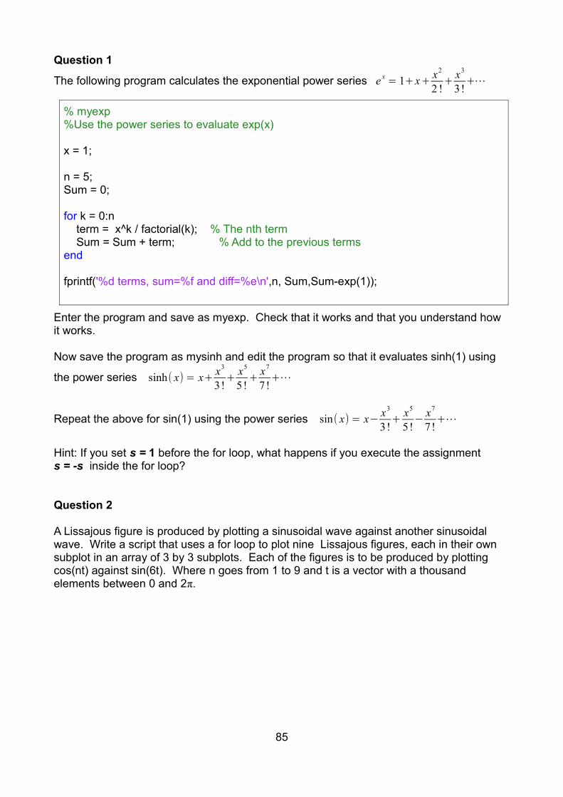
Question 1

The following program calculates the exponential power series e x = 1+x+ x2

2 !+x3

3!+⋯

Enter the program and save as myexp. Check that it works and that you understand how it works.

Now save the program as mysinh and edit the program so that it evaluates sinh(1) using

the power series sinh( x) = x+ x3

3!+x5

5!+x7

7!+⋯

Repeat the above for sin(1) using the power series sin( x) = x− x3

3!+x5

5!−x7

7!+⋯

Hint: If you set s = 1 before the for loop, what happens if you execute the assignment s = -s inside the for loop?

Question 2

A Lissajous figure is produced by plotting a sinusoidal wave against another sinusoidal wave. Write a script that uses a for loop to plot nine Lissajous figures, each in their own subplot in an array of 3 by 3 subplots. Each of the figures is to be produced by plotting cos(nt) against sin(6t). Where n goes from 1 to 9 and t is a vector with a thousand elements between 0 and 2π.

85

% myexp%Use the power series to evaluate exp(x) x = 1; n = 5;Sum = 0; for k = 0:n term = x^k / factorial(k); % The nth term Sum = Sum + term; % Add to the previous termsend fprintf('%d terms, sum=%f and diff=%e\n',n, Sum,Sum-exp(1));

Accessing array elements using a loop

Often the loop variable in a for loop is used to access the the kth element of an array. For example, enter the following into a script called graph2.m

The function called length tells us the length of the vector x. So the loop goes round for k = 1, then 2, then 3, up to n. Each time around the loop, we read the kth value of x and use it to calculate the kth value of y .

In many programming languages, this is the only way to populate an array. In Matlab it is easier and much more efficient to do this :-

There are however situations when a loop has to be used.

ExampleThe Fibonacci sequence is defined by

F1=0

F2=1

F n+1=F n + Fn−1Find the first 20 terms of the sequence.

86

x = linspace(0,2*pi,100);

n = length(x); for k = 1:n y(k) = cos(x(k));end plot(x,y)

x = linspace(0,2*pi,100);y = cos(x);plot(x,y)

%The Fibonacci sequencen = 20; % number of termsF = zeros(1,n); % reserve space for F F(1) = 0; % 1st termF(2) = 1; % 2nd term for k = 2:n-1 % The remaining n-2 terms F(k+1) = F(k) + F(k-1); % The recurrence relation fprintf(' %d %d \n', k+1, F(k+1))end

Notice that the variable F is created with the correct dimensions, at the top of the script. The function zeros is used to do this. If the zeros function is removed, the size of the vector will increase by one, each time around the loop. To do this, MATLAB has to create a new space in memory to hold the variable, then copy the content of the variable into the new memory space.

It is not absolutely necessary to create a variable of the correct size, but it does make the program run faster.

Also notice that the program output is not very neat. The columns do not line up because some output lines require more space for the larger numbers. This is why it is sometimes useful specify the width in fprintf. Change the fprint line in the script to the following.

This sets the width of each column to 6 characters. You can give each column a name.Add the following line to the beginning on the script.

See if you can also print out a row when k =1 and when k = 2.

Question 3A sequence is defined by the following recurrence relationship

f 1=0

f 2=0.0628

f n+1=1.996 f n − f n−1Find the first 100 terms of the sequence and plot f.

87

fprintf(' %6d %6d \n', k+1, F(k+1))

fprintf(' %6s %6s \n', 'k', 'F')

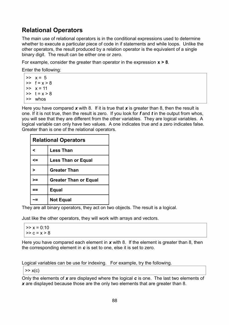
Relational OperatorsThe main use of relational operators is in the conditional expressions used to determine whether to execute a particular piece of code in if statements and while loops. Unlike the other operators, the result produced by a relation operator is the equivalent of a single binary digit. The result can be either one or zero.

For example, consider the greater than operator in the expression x > 8.

Enter the following:

Here you have compared x with 8. If it is true that x is greater than 8, then the result is one. If it is not true, then the result is zero. If you look for f and t in the output from whos, you will see that they are different from the other variables. They are logical variables. A logical variable can only have two values. A one indicates true and a zero indicates false. Greater than is one of the relational operators.

Relational Operators

< Less Than

<= Less Than or Equal

> Greater Than

>= Greater Than or Equal

== Equal

~= Not Equal

They are all binary operators, they act on two objects. The result is a logical.

Just like the other operators, they will work with arrays and vectors.

Here you have compared each element in x with 8. If the element is greater than 8, then the corresponding element in c is set to one, else it is set to zero.

Logical variables can be use for indexing. For example, try the following.

Only the elements of x are displayed where the logical c is one. The last two elements of x are displayed because those are the only two elements that are greater than 8.

88

>> x = 5>> f = x > 8>> x = 11>> t = x > 8>> whos

>> x = 0:10>> c = x > 8

>> x(c)

There is no need for a separate logical variable. The logical expression can be placed directly in the round brackets.

You need to use a double equals sign to avoid confusion with an assignment.

x=8 Assigns the value 8 to x.

x==8 Compares the value 8 with x.It is very common to forget to use a double equals for a comparison.

You can compare two characters using the == relational operator.

There are two function to compare two strings

>> strcmp('Yes','yes') Is case sensitive.

>> strcmpi('Yes','yes') Is case insensitive.

There are also logical operators that are used to combine logical variables.

Logical Operators

& AND

| OR

~ NOT

>> x(x>=4 & x<8) x>=4 AND x<8

>> x(x<=4 | x>8) x<=4 OR x>8

Use shift \ to get the vertical line.

>> x(~(x>=8)) NOT (x >=8)

You need to use brackets with the NOT operator. If you do not use brackets, the NOT is applied to just x instead of the expression x >=8. To see why, enter :-

89

>> x(x>8)>> x(x<8)>> x(x==8)

>> doc operator precedence

>> a = 'P'>> a == 'P'>> a == 'p'

Common Mistakes

>> x== 4 | 8 Will not work.

Logical operators only act on logical variables. They do not work for numbers.

If you want to test if x is 4 or 8 use.

>> x== 4 | x == 8

Here or is operating on two logicals. The result of x==4 and the result of x==8.

>> 4 < x < 8 Will not work.

This will always be true, regardless of the value of x. 4 < x will be either one or zero. Both are less than 8.

To test if x is between 4 and 8 use.

>> 4 < x & x < 8

Example

Plot f (x) for −5 ≤ x ≤ 5

when f (x) = {x+3, x ≥ 0x , x < 0.

Question 4Plot f (x) for −5 ≤ x ≤ 5

when f (x) = { x2 , x ≥ 1x , −1< x < 1

−x 2 , x ≤−1.

90

x = -5:0.01:5; f = x + 3; p = x < 0; % p is a logical that is true when x<0f(p) = x(p); % Operate only on the points where x < 0 plot(x,f)

Conditional Execution (The IF statement) The simplest form of an if statement is as follows.

The if statement consists of a block of statements which is enclosedbetween if and end, and a condition in round brackets. The block ofstatements is only executed if the condition is true.

As an example, enter the following script into wave.m.

Run the script and observe the plot.

91

if (condition)statement1statement2

end

%wave%produce a waveform n = 100; % Size of the output x = 0;Y = zeros(n,1); % create vector for result for k = 1:n x = x + 1; % count up if (x == 8) x = 0; % reset to zero at 8 end Y(k) = x; % Store result into a vectorend plot(Y)

condition

statement1

statement2

True

False

Slightly more advanced is the if else statement.

Where block1 is executed if the condition is true and block2 isexecuted if the condition is false.

Edit the script wave. Replace

with

Run the script. This time you should get a triangular wave. Single step through the script, if you want to.

ExampleWrite the code below into a script

92

if (condition)statement block1

elsestatement block2

end

condition

statement1.1

statement1.2

True

False

statement2.1

statement2.2

if ( x<4) Y(k) = x; else Y(k) = 8-x; end

Y(k) = x; % Store result into a vector

% Create a question dialogue box.

T = 'A Silly Question'; % The dialogue box titleQ = 'Do you understand this program'; % The question being asked

answer = questdlg(Q,T) % Leave the semicolon off if (strcmp(answer,'Yes')) % If the answer is Yes message = 'Move on to the next part';else message = 'Ask a demonstrator for help';end msgbox(message); % Display the message

While loops The while loop is a conditional loop.

A while loop will keep looping WHILE the condition is true. At theend of each loop, the while loop returns to the top of the loop andtests the condition. If the condition is true, it will loop again. If thecondition is false, it jumps to the MATLAB code after the end at thebottom of the loop.

ExampleHow long does it take for prices to double when the inflation rate is2% per year ?

Use the following script to find the solution.

We could have used a FOR loop, but we would have had to make an estimate of the number of loops required. That is the main difference between a FOR and WHILE loop. We know exactly how many loops a FOR loop will do before we run the program. A WHILE loop can be adjusted to the the number of loops required.

If the condition is never true, then the WHILE loop will loop forever. To stop a run away WHILE loop:

• Click into the command window.• Hold down the ctrl key and press c. You may have to do this several times.

Change 1.02 to .999 in the above script and try this now.

93

while (condition)statement1statement2 ...

end

condition

statement

statement

True

False

% Time for prices to double with 2% inflation.

price = 1; % The initial cost of the itemyear = 0; % the time in years fprintf('\t Years \t Price \n\n'); %The column headers while (price < 2) price = price * 1.02; %Increase the price by 2% year = year + 1; %Increase the year by one fprintf('\t %-4d \t %0.2f \n',year,price); %Add the next row to the table end

IterationIteration is a mathematical procedure for solving equations. For example, to solve the equation

x − cos( x)= 0 (1)

We could rearrange the equation to give x.x = cos( x) (2)

Guess the value of x, then repeatedly recalculate equation (2) and hope the value of x getscloser to the correct solution.

A while loop is a natural choice to implement an iteration program.

Write the above into a script and see how many steps are required to get an acceptable solution.

If the function you are trying to solve is differentiable, then the Newton Raphson method is an extremely good way of finding a solution.

If f (x) = 0 then iterate with x = x−f ( x )f ' (x )

For the problem above

x = x−x − cos( x)1 + sin( x)

Change the program above to solve the problem using the Newton Raphson method.

Question 5Write a script to solve x2−7=0 , using the Newton Raphson method.

94

% solve the equation x - cos(x) = 0 x = 0; % The initial value of xk = 0; % The number of iterationserr = 1; % The initial error to get things started while (err >= 1e-6) x = cos(x); %find the next x. err = abs(cos(x) - x); % calculate the error k = k + 1; %Increase number of iterations by 1 fprintf('\t %-4d \t %0.7f \t %0.5e \n',k,x,err); %Display results so far end

Functions You may want to run your program many times with different values. It is cumbersome to have to edit the script every time you use a different number. What is required is a piece of code that you can run at will (as with a script), but where at the same time you can specify the values to use for the calculation. This is the precisely the role of a function in MATLAB and other programming languages. You have already used inbuilt functions like sin(x). Now it is time for you to write your own functions.

Functions, like scripts, are a succession of MATLAB statements stored in a text file. However, there are important differences. A function has a specified number of inputs andoutputs. For example, look at the function below.

The first line of the file tells MATLAB that we are about to define a function by using the function keyword and declares what the input and output of the function are called.

F2C is the name of the function. This should be the same as the file name.

F is the input into the function. In this case it is the temperature in Fahrenheit. This is called an input parameter or argument. A function can have zero, one or many input arguments.

C is the output from the function. In this case the temperature in Centigrade. This is called the return value.

Enter the above function into a file called F2C.m. Then in the command window, enter the following :-

95

function C = F2C(F)%Temperature conversion, Fahrenheit to Centigrade. C = (F - 32)*5/9;

>> F2C(212)>> x = 68>> y = F2C(x)>> F2C(59) + F2C(77)>> F2C(x^2)>> (F2C(x))^2>> t = F2C(10 + 7^2)>> help F2C

>> f = 32:9:212>> c = F2C(f)>> plot(c,f)

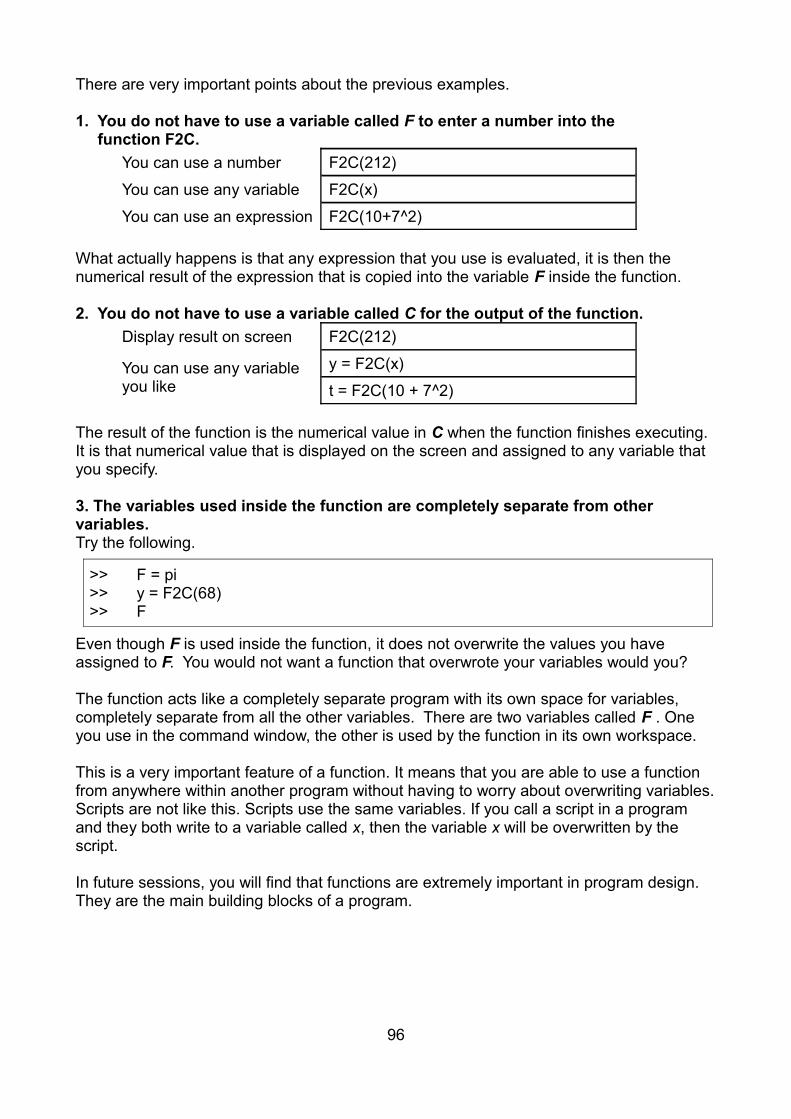
There are very important points about the previous examples.

1. You do not have to use a variable called F to enter a number into the function F2C.

You can use a number F2C(212)

You can use any variable F2C(x)

You can use an expression F2C(10+7^2)

What actually happens is that any expression that you use is evaluated, it is then the numerical result of the expression that is copied into the variable F inside the function.

2. You do not have to use a variable called C for the output of the function.

Display result on screen F2C(212)

You can use any variable you like

y = F2C(x)

t = F2C(10 + 7^2)

The result of the function is the numerical value in C when the function finishes executing. It is that numerical value that is displayed on the screen and assigned to any variable that you specify.

3. The variables used inside the function are completely separate from other variables.Try the following.

Even though F is used inside the function, it does not overwrite the values you have assigned to F. You would not want a function that overwrote your variables would you?

The function acts like a completely separate program with its own space for variables, completely separate from all the other variables. There are two variables called F . One you use in the command window, the other is used by the function in its own workspace. This is a very important feature of a function. It means that you are able to use a function from anywhere within another program without having to worry about overwriting variables.Scripts are not like this. Scripts use the same variables. If you call a script in a program and they both write to a variable called x, then the variable x will be overwritten by the script.

In future sessions, you will find that functions are extremely important in program design. They are the main building blocks of a program.

96

>> F = pi>> y = F2C(68)>> F

How t = F2C(10 + 7^2) is evaluated.

10 + 7^2 The input expression is evaluated.

59 The numerical value of the expression is passed to the function.

The function is like a self contained program. It cannot read or write to any variables outside the function.

F2C

15 The function returns the numerical result.

t The result is copied into the variable.

The consequences of this are 1. You cannot set a variable in the command window or a script and use it inside a

function.

2. You cannot set a variable inside a function and use it in the command window or a script.

3. You should only use input parameters to get numbers into a function.

4. Only use return values to get numbers back from a function.

Question 6Write a function called C2F that converts Centigrade to Fahrenheit.

Question 7(a) Covert the script you wrote for question 5 into a function to find the solution of

x2−A=0

Where A is an input argument to the function and the solution x is the returned value.Call the function mysqrt.m I hope that you can see that x will be the square root of A. A must be a positive number.

(b) Write a script that uses mysqrt in a for loop to evaluate all the square roots of all the integers from one to one hundred. Then plot them in a graph.

97

Functions with more than one argument

Enter the function below.

To avoid confusion, always store a function in a file with the same name as the function. So in this case, save the function into a file called fn.m. Try the following.

If you don't understand this, try putting in a break point and see what is copied into a and b.The first expression is copied into the first argument a, the second expression is copied into the second argument b. It is the order in which the expressions are entered that determines which parameter they are used for, not the variable name that you use.Try these

Functions with more than one output

In most programming languages, a function can only return one item. MATLAB functions also only return one item, but that item can be an array of variables. Change the function fn so that it returns two numbers in an array.

Then try the following

It is the order of the variables, not their names that determines what result is copied into which variable. In this case, the sum is copied to the first variable and the difference is copied to the second. If you do not provided a second variable, only the sum, the first variable is returned.

98

function diff = fn(a,b)diff = a - b;

>> a = 4>> b = 1>> s = fn(a,b)>> s = fn(b,a)

>> x = 2;>> s = fn(x^3,x^2)>> s = fn(1:10,1)

function [sum diff] = fn(a,b)sum = a + b;diff = a - b;

>> [s,d] = fn(5,4)>> fn(5,4)>> s = fn(5,4)>> [x,y] = fn(5,4)

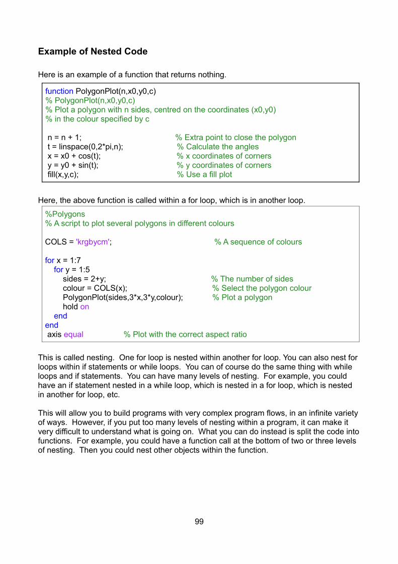
Example of Nested Code

Here is an example of a function that returns nothing.

Here, the above function is called within a for loop, which is in another loop.

This is called nesting. One for loop is nested within another for loop. You can also nest for loops within if statements or while loops. You can of course do the same thing with while loops and if statements. You can have many levels of nesting. For example, you could have an if statement nested in a while loop, which is nested in a for loop, which is nested in another for loop, etc.

This will allow you to build programs with very complex program flows, in an infinite varietyof ways. However, if you put too many levels of nesting within a program, it can make it very difficult to understand what is going on. What you can do instead is split the code intofunctions. For example, you could have a function call at the bottom of two or three levels of nesting. Then you could nest other objects within the function.

99

function PolygonPlot(n,x0,y0,c)% PolygonPlot(n,x0,y0,c)% Plot a polygon with n sides, centred on the coordinates (x0,y0)% in the colour specified by c n = n + 1; % Extra point to close the polygon t = linspace(0,2*pi,n); % Calculate the angles x = x0 + cos(t); % x coordinates of corners y = y0 + sin(t); % y coordinates of corners fill(x,y,c); % Use a fill plot

%Polygons% A script to plot several polygons in different colours COLS = 'krgbycm'; % A sequence of colours for x = 1:7 for y = 1:5 sides = 2+y; % The number of sides colour = COLS(x); % Select the polygon colour PolygonPlot(sides,3*x,3*y,colour); % Plot a polygon hold on endend axis equal % Plot with the correct aspect ratio

Session 2 Exercises

The objective of these exercises is to write a program that includes animated shapes moving about the screen. You can choose what the program actually does. It could be a very simple game, a simulation or just an animated pattern.

Before you write your program, you are going to write a set of functions that will make writing your program easier. A common programming technique is to define your own datatype and then write a set of functions that will do what you need to do with the data.

The data type you are going to use, we will call a shape. The data consists of a set of coordinates that describe a path around the outside of a shape. In exercise 1, you write afunction to draw a shape onto a graph. Then you write a set of functions to perform graphical transformations. Graphical transformations move objects around a graph, while maintaining their size and shape. You are going to write functions to perform translation, reflection and rotation.

The shape is going to be stored in a 2 by n matrix. Take for example the arrow below :-

This is represented by the matrix.

[0 1 1 3 3 1 1 00 1 1 /2 1 /2 −1/2 −1/2 −1 0]

• The x coordinates are on the top row of the matrix. • The y coordinates are on the bottom row.• Each column represents the coordinates of a point on the arrow.

The first column is the point at the tip of the arrow. The second column is the next point moving clockwise around the arrow. The third column is the next point after that and so on, moving around the arrow to define the path of the perimeter of the arrow. The very lastcoordinate returns to the arrow tip again to close the shape.

100

(1,1)

(1,-1)

(1,-1/2)

(1,1/2)

(0,0)

(3,-1/2)

(3,1/2)

Exercise 1

(a) Create a new directory to contain all your programs associated with this set of exercises.In the new directory, write a function that given the matrix of the path around the outside ofa shape, will plot the object. Name the function drawshape.

• The function should have one input, the shape to draw, such as the matrix of the arrow.

• No title or other graphic annotation are required in this function. You will understand why later.

• The function will plot the shape and return nothing.

• The function must be able to plot different shapes with a different numbers of points.

So to draw a shape, you would enter :-

Hint: You just need to plot the x and y coordinates. See indexing in session 1.

(b)Write a script called transform, that draws an arrow. The script should do two things

• Assign the arrow matrix to a variable.

• Draws the shape in the variable using drawshape.

Try creating and drawing a square. Don't remove the arrow matrix, you will need it later.

(c)Add a second argument c to the function drawshape to set the line colour of the shape.Hint: Look at the function PolyPlot in the example before the exercises.

Edit the script transform so that it contains something like :-

101

>> drawshape(shape)

>> drawshape(shape,'g')

Exercise 2

(a)A translation moves an object to a new location. It maps the original origin to a point (a, b). Write a function called translate that translates the shape to (a, b).

• The function should have three arguments, the shape to move, a and b.

• The function should return the new translated shape.

• The function MUST NOT plot the translated shape.

The functions that perform the transformations must not draw the shapes. Later we will beperforming several transforms on a shape before using drawshape to plot the result.

Hint: By now you should know how to extract the x and y coordinates. Add a to x and b to y. Then reform the new shape matrix. How can you make a two row matrix from two row vectors ?Think back to session 1.

(b)Edit the script transform. At the bottom of the script, use the function that you wrote for part (a) to translate the arrow to (2, 3). Then use drawshape to draw the new arrow in red, still showing the original arrow in green.

102

Exercise 3

(a)Write a new function called reflectx, to reflect a shape about the x axis.

• The function should have one argument, the shape to reflect.

• The function should return the new reflected shape.

You can do this with matrix multiplication. newshape= [1 00 −1] × shape

(b)Write a new function called reflecty, to reflect a shape about the y axis.

The equation this time is newshape= [−1 00 1] × shape

(c)Write a third function just called reflect. This will have two inputs. The shape and a character variable. When the character is x, it will use reflectx to reflect the shape, otherwise it will use reflecty.

(d)In transform, use the function defined in part (c) to reflect the translated shape (the shape that was drawn in red in exercise 2) about the y axis and draw it in cyan. Then reflect it again about the x axis and draw it in magenta.

At this stage, I suggest that you add the following to the bottom of the script to force MATLAB to scale properly.

(e)Edit the file reflect.m. At the very end of the file, below everything else, copy the entire contents of the file reflectx.m. Below that copy the the entire contents of reflecty.m.

Rename the file reflectx.m to OLDreflectx.m and reflecty.m to OLDreflecty.m. Run transform again to make sure that everything still works.

The two functions reflectx and reflecty are now “Local” functions, defined at the end of reflect. The advantage is that this has reduced the number of files. The disadvantage is that reflectx and reflecty can now ONLY be called in the function reflect, not in the command window or in any other script or function.

(f)Change reflect so the both lower case x and capital X will select reflection about the x-axis.

103

axis([-10 10 -10 10])axis square

Exercise 4

(a)The last of our fundamental transformations is a rotation. Write a function called rotate that returns a shape rotated about the origin by angle a, an input. It is very similar to a reflectx, but with a different matrix.

newshape= [cos(a) −sin (a)sin (a) cos(a) ] × shape

(b)In transform, rotate the last shape by π/4 and draw it in blue.

Exercise 5

More complex transformations can be performed using combinations of the fundamental transformations.

(a)Write a function called rotateabout which rotates by an angle a about a specified coordinate (x , y).

This can be easily achieved by using the functions translate and rotate.Use these functions to :

• Translate the shape to (-x , -y ).

• Rotate by a.

• Translate to (x , y ).

(b)Write a new script called transform2 that rotates the original arrow about (1.5,-4), n times.Each copy rotated by a different angle, evenly distributed between 0 and 2π. Where n is a variable.

104

Exercise 6

Now we can animate the motion, by displaying just one arrow at a time for a short period. In transform2 :-

• Remove any hold commands.

• Move the axis commands inside the loop.

• Add the following to the end of the loop :-

drawnow forces the graph to display now, without waiting for any further graphics commands.

pause(0.1) waits 0.1 seconds.

For smoother animation, make n larger and the pause shorter.

105

drawnowpause(0.1)

Exercise 7

Use the functions developed in the previous exercise in your own program. You can produce your own shapes. You can place them where you like and you can move them around. It can be a very simple game or a simulation or just produce a complex pattern or an animation. What the program does is your choice. Please, nothing offensive or tasteless.

This is your opportunity to show us what you can do. Start with something simple, then you can develop it into something more complex if you wish.

For those that have the time and want to put a bit more into their program.

• You can make shapes larger or smaller by multiplying the matrix by a constant.

• If you want solid shapes, replace plot with fill .

• In addition to the single letter colour codes used by plot, the fill command can also take a row vector containing the amount of red, green and blue. MATLAB also has functions that return a sequence of n colours. For example gray(64), summer(50), cool(100). There is an example of how to use the cool function on the next page.See doc colormap for more maps.

• More elaborate shapes can be produced by functions. For example, a regular polygon function could be used to produce a circle. See the function on the next page.

• If you want text, you can use the function text(x,y,'my text').

• [x ,y , button] = ginput(1) waits for a mouse button press on the graph. ◦ (x,y) is the coordinates of the mouse pointer. ◦ button is either 1, 2 or 3 for left, middle or right mouse buttons. See the example on the next page.

It is NOT compulsory to put any item from the above list into you program.

To get top marks for this session, you need to show that you have developed your own ideas into a working program.

Assessment 2

Now ask to be assessed. You will be assessed on your results for the exercises, but you may be asked the odd question to test your proficiency.

106

Example of using the cool function

A polygon generating function

Example of how to use ginput

107

% draw n triangles, each with a slightly different colourshape = [0 2 1 0 ; 0 0 2 0] ; % A triangle n = 20; % Number of trianglesY = linspace(0,40,n); % Y coordinatescolours = cool(n); % n different colours for k = 1:n shape1 = translate(shape,0,Y(k)); col = colours(k,:); %Each colour is a row of the matrix. fillshape(shape1,col) % col will only work with fill hold onendaxis equal

%function shape = polygon(r,n)% generate a regular n sided polygon of radius r. t = linspace(0,2*pi,n+1);x = r * cos(t);y = r * sin(t); shape = [ x ; y];

%function shape = polygon(r,n)% generate a regular n sided polygon of radius r. t = linspace(0,2*pi,n+1);x = r * cos(t);y = r * sin(t); shape = [ x ; y];

% left mouse button draws a triangle, right button to quit.shape = [0 2 1 0 ; 0 0 2 0] ; % A triangle axis([-10 10 -10 10])hold on[x,y,button] = ginput(1); %find coordinates of pointer while (button == 1) %While left mouse button used shape1 = translate(shape,x,y); %Move shape to pointer drawshape(shape1,'g') %draw shape [x,y,button] = ginput(1); %Get next coordinateend

108

Session 3

DBT Part A: Simulating a Rocket Launch

Introduction In the remaining sessions 3-5, you will reinforce and apply what you have learnt in sessions 1-2 in a more open-ended Design, Build and Test project. Your tasks are to build simulators for the launch of a Saturn V rocket and for the landing of a interplanetary probe.

DebuggingYou will learn how to write large complicated programs. If you have a large program, debugging is where things can go badly wrong. It is very easy to become completely overwhelmed by a program if care is not taken. Suppose that you write a MATLAB script with approximately a thousand lines of code. What do you think are the chances of writinga thousand lines of code with out any mistakes? There are bound to be spelling errors, syntax errors or things that are just wrong. In general, the larger the program, the more errors there will be.

It can be difficult to find an error in a few lines of code. Can you imagine how much more difficult it is going to be to find an error in a thousand lines of code? Using the debugger will not be easy. Single stepping through a thousand lines is going to be very tedious. There are bound to be loops that will increase the steps required.

So not only do you have a lot of errors, it is going to very difficult to find each error. The larger the program, the more difficult and time consuming it gets. This is a very serious problem. In the worst case scenario, you never finish the program. It just becomes too difficult to work on.

In practice, you don't even attempt to debug hundreds of lines of code in one go. Instead you split the program into separate functions. Each function is tested and debugged separately. For example, you could split a thousand lines of code into 5 functions. It does not have to be an even split, but lets assume for simplicity that each function has about 200 lines of code. That is still a lot of code to debug, so we split the functions again and again until each function has a sufficiently small amount of code.

There will probably be over a hundred functions, so it will still take a long time to write. However, as you will be testing each function separately, at the lower level you will only be debugging ten to twenty lines of code at a time. That is going to be much easier than debugging a thousand lines of code. At higher levels, the functions will consist mostly of calls to functions at a lower level. Provided that each of these lower functions has been tested already, they should be fairly easy to debug.

109

f4()f5()

f3()f2()f1()

f34()f33()f32()f31()

f3()f2()f1()

f35()f324()f323()f322()f321()

Using functions makes it much easier to single step through the program. At each functioncall you have the choice of executing the whole function as a single step or stepping into the function and stepping through the function line by line. By stepping over the majority ofthe functions, you can easily home in on any part of the program in a few steps.

Program IntelligibilityIf you have a program with hundreds of functions, you will not be able to keep a detailed description of each function in your head. If you return to a function after several weeks, you do not want to waste time working out how the function works all over again. It does not help if your program looks like gobbledygook. The neatness and clarity of your code are much more than optional “window dressing”.

Add comments to your code. Adopting a consistent style will clarify your thinking, and will make it easier for other people to understand your code.

• Use variable names which convey some meaning to the reader: a1, a2, a3 are rarely the best choices of name! (But don't use over long names either.)

• Code indentation makes code easy to read. MATLAB will do this for you. In the editor, right click and choose Select All. On the icon bar, under the EDITOR tab, you will find the Smart Indent icon. This is the icon, just to the left of the word indent.

• Insert empty lines to break up blocks of code. Use comments to indicate the purpose of a block of code. Add more detailed comments to a particular line if it is noteworthy.

• Avoid stating the obvious. “This line adds a and b" is not helpful. You don't have to add a comment on every line.

• If you have comments on the same line as program code, try to keep them separate.

• When you use help on your program or function, it should be clear what it does and how to use it.

• If you find yourself repeating code it should probably be put into in a function.

• Don't bury “magic numbers” in your code. If your code needs constants declare them at the top of the file and assign them to variables names. This way you won't have constant numbers appearing all over your code, which if you need to change will undoubtedly lead to misery. It is very easy to miss a constant assignment deep within your code.

110

Top Down DesignTop down design helps you to break down a program into smaller functions. It can also make your program more readable.

A top down design is written in plain English. You start by putting in a title. Then you write down and number the main steps that the program needs to carry out. These steps need to be very broad. You do not want too much detail at the top level. You are aiming for a minimal number of steps.

Then you look at each step in turn and try to split it up into simpler steps. For example step one could be split in step 1.1, 1.2, 1.3 and step 1.4. When you have done this for all the steps on the top level, you repeat the procedure for the steps at the next level down. For example, step 1.3 could be split into step 1.3.1 and step 1.3.2.

Program to draw a person

1 Draw head 2 Draw body 3 Draw legs 4 Draw arms

Program to draw a person

1 Draw head 1.1 Draw circle 1.2 Draw mouth 1.3 Draw eyes 1.4 Draw nose 2 Draw body 3 Draw legs 4 Draw arms

Program to draw a person

1 Draw head 1.1 Draw circle 1.2 Draw mouth 1.3 Draw eyes 1.3.1 Draw left eye 1.3.2 Draw right eye 1.4 Draw nose 2 Draw body 3 Draw legs 4 Draw arms

You continue to do this until your steps are sufficiently simple to convert into code.

The Design CycleTo make things easier, we are going to start with the simplest designwe can. Then after we have that working, we return to the designstage and make the design a little bit more complex. We keep goingaround the loop until the design does everything we want.

This is called the design cycle. The idea is that we make it easier totest and debug the code by added the minimum amount of code to theprogram in each cycle. Testing simple mathematical models is easierthan more complex models. So some of the code can be validatedusing simple tests.

The design cycle can be applied to the whole program or any of thefunctions.

111

Design

Build

Test

Debug

TestingYou should test code as you go along. When youhave written a function, check that it behaves asexpected. When all your code appears to “work”,stress-test it by changing input parameters,checking that the output changes as expected.Regard the code not as an end in itself, but ratheras a piece of apparatus that allows you to performexperiments.

Your testing should be rigorous. If there are severaldifferent paths which the code can take within thefunction, you have to make sure that each differentpath is tested. For example, in the flow chart on theright, the code in blocks A to F must each be tested.

Backing up your programEven the best programmers occasionally completely mess up a working program. You need to make sure that if this happens, you have saved the working version of your program.

Suppose you are developing your program in a folder called Rocket. First create a folder inside Rocket called version1. Write your program within the version1 folder. Then when you have completed the first design cycle, copy the whole of version1 directory to a new directory. Rename the directory version2.

You can do this by cut and paste in the Current Folder window in MATLAB. • Go to the Rocket folder• Select version1, then right click and select Copy.• then right click again and select Paste. • then select the copied directory and right click again and select Rename.

An alternative is to use a terminal window. You would enter.

If you still have the editor open, you will probably still have version1 programs open. To avoid confusion, shut down the editor. Double click on the version2 directory. Then double click on any files that you want to open. Then carry on working in version2.

But if the major rewrite you make turns out to be a big mistake then you still have a copy ofthe original version1. So you would then copy version1 to version3. Notice that the disaster version2 is not immediately deleted. Never delete in haste. You may find later thatversion2 was not such a big mistake after all.

The logical organization of your file store (folder structure, folder and file names) is just as important as the logical organization of your program.

112

cp -r version1 version2

A D

B C

E

F

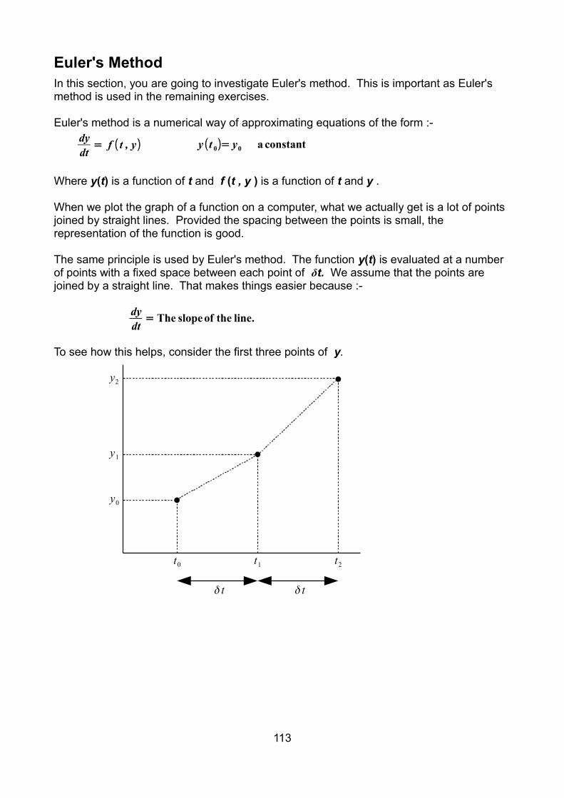
Euler's Method In this section, you are going to investigate Euler's method. This is important as Euler's method is used in the remaining exercises.

Euler's method is a numerical way of approximating equations of the form :- dydt

= f ( t , y) y (t 0)= y0 a constant

Where y(t) is a function of t and f (t , y ) is a function of t and y .

When we plot the graph of a function on a computer, what we actually get is a lot of points joined by straight lines. Provided the spacing between the points is small, the representation of the function is good.

The same principle is used by Euler's method. The function y(t) is evaluated at a number of points with a fixed space between each point of δt. We assume that the points are joined by a straight line. That makes things easier because :-

dydt

= The slopeof the line.

To see how this helps, consider the first three points of y.

113

t0 t1

δ t

y0

y1

t2

y2

δ t

We know the value of the y0, that was given in the original problem. The first objective is to find y1.

We also know

f (t 0, y0) =dydt

(1) From the original problem.

dydt

= Slope (2)Because the derivative of a straight line is the slope of the line.

Slope=y1 − y0

δ t(3) The basic definition of the slope of a straight line.

Putting (1), (2) and (3) together we get.

f (t 0, y0) =dydt

= slope =y1 − y0

δ t

f (t 0, y0) =y1 − y0

δ t(4)

The only unknown is y1, so rearranging (4) in terms of y1, we gety1 = y0 + δ t f ( t0, y0) (5)

So now that we know y1, we can use the same procedure to find y2.y2 = y1 + δ t f ( t1, y1)

And so on. y3 = y2 + δ t f ( t 2, y2)

In general. yk+1 = yk + δ t f (t k , yk) (6)

On the next few pages is an example of how to use Euler's method to solve a differential equation. Read through the example and then try the questions on page 117.

114

Top Down Design of Euler's Method

Using Euler's method to solve y'(t) = f(t,y) y(0) = y0

1. Initialise the values.

2. Repeat for each time step.

3. Store the current values for plotting later.

4. Evaluate the current value of f(t,y).

5. User Euler's formula to evaluate y for the next step. y = y + dt*f(t,y)

6. End of repeat.

7. Plot the data.

Example(a) Use the top down design of Euler's method to write a program that solves.

dydt

= f ( t , y) =− y y (0)= y0=1

For 0 ≤t ≤ 1 with a step size δ t = 0.1

(b) Compare the solution above with the analytic solution.

y (t )=e−t

115

%Using Euler's method to solve y'(t) = f(t,y) y(0) = y0 %1. Initialise the values% 1.1 set the initial value of y.y = 1; % 1.2 set the start and end value of ttstart = 0;tend = 1; % 1.3 set the step size (using dt for delta t)dt = 0.1;

Notice that the program itself contains the top down design as comments. If you have a top down design, start your program by writing the top down design into your program as comments. Then you add the code after each comment. This means you have a very good description of what the codes does, even before you start to write the code. It is much easier than trying to describe what the code does after you have written it.

116

% 1.4 Initialise vectors to store the data to plotT = tstart:dt:tend; % Vector of values of t.n = length(T); % Find the total number of pointY = zeros(1,n); % Vector to store the values of y. %2. Repeat for each time stepfor k = 1:n %3. Store the current values for plotting later Y(k) = y; %4. Evaluate the current value of f(t,y) f = -y; %5. User Euler's formula to evaluate y for the next step y = y + dt*f; end %6. End repeat %7. Plot the dataplot(T,Y,'r') xlabel('t')ylabel('y')grid %Plot the analytic solution as a comparison Y2 = exp(-T);hold onplot(T,Y2,'b'); legend({'Euler's Method','Actual value'})

Question 1Enter the example code and test the program. Try changing the step size 0.01 and see if you get a better results.

The approximation works if the step size δt, is small. If the step size is too large, the approximation will not hold and the error will be large. To keep the error small, you use lotsof small steps.

Question 2(a) Write a program that solves.

dydt

= f ( t , y) = cos( t) y (0)= y0=0

For 0 ≤t ≤ 2π with a step size δ t = 0.01

(b) Compare the solution above with the analytic solution.y (t )=sin( t )

Hint : To start, copy the previous program.

Question 3(a) The velocity of the object dropped from hight is defined by the differential equation

dvdt

= g−cmv2 v (0)=0

Where

The acceleration due to gravity g = 9.81 m/s2

The drag constant c = 0.3 Ns2/m2

The mass m = 80 kg

Write a program that uses Euler's method to calculate the velocity of the object.For 0 ≤t ≤ 25 with a step size δ t = 0.01

(b) Use the data cursor to measure the velocity after 25 seconds. The velocity should approach, but not be greater than the terminal velocity.

dvdt

is zero when v = terminal velocity.

Calculate the terminal velocity and compare it with v(25).

117

Modelling Dynamic Systems

We are now going to model a ball thrown vertically upwards.

y = the height of the ballv = the velocity of the balla = the acceleration of the ball

This time we need to solve two differential equations for each step. dydt

= v dvdt

= a

That means that that we need to use equation (6) twice. So the top down design looks like this.

Using Euler's Method to Plot a Ball Thrown Upwards.

1. Initialise the values

2. Repeat for each time step

3. Store the current values of both y and v for plotting later

4. Use Euler's method to find the position at the next step y = y + dt * v

5. Use Euler's method to find the velocity at the next step v = v + dt * a

6. End of repeat

7. Plot the data

Question 4Use the above top down design to write a program to plot the velocity and height of the ball.

• The acceleration is a constant a = -9.81 m/s2 . • The initial value of v = 25 m/s . • The initial value of y = 0.

Plot both v and y in separate graphs on the same figure. Each graph should be labelled.

The height should be an inverted parabola. The ball should hit the ground before 6 seconds.

118

A principle of Euler's method is that :-

Use the values of the variablesat step k → To predict the the values of the

variables at the next stepk+1

That is why the value of y is calculated in item 4, before v is calculated in item 5, in the topdown design. If the two items were placed in the opposite order, then the new value of v would be used to calculate the new value of y.

In the ball simulation, if the step size is small, the order in which you calculate v and y is not going to make much difference to the result. However, it is a good principle to stick to. In the exercises that follow and those in the next two sessions, there are a lot more variables. It can get very confusing about what is being used to calculate what. It is easy to get into circular argument, if you are not careful.

119

Simulating a Rocket Launch

Initial Mass 2900 tonnes

Total Thrust at Launch

34000 kN

Stage 1 Burn Time 150 s

Stage 1 Propellant Mass

2,150,000 kg

Max Diameter 10 m

Length 110 m

The Saturn V rocket used in the Apollo 11 Mission, and some of the flight parameters.

For the remainder of this session, you are going to write a program to simulate the launch of a Saturn V rocket. The Saturn V rocket is the largest rocket ever built. It was used for the first manned missions to the moon. The table above gives some specifications of a typical Saturn V rocket (read these carefully, it was a monster).

You are given a top down design of the program. In the exercises that follow, you will produce the program code using the top down design.

There is no mark for session 3, but your work will still be assessed by a demonstrator to provide feedback on your software. This will show you where you would have lost marks and help you understand how to get good marks in your final assessment, at the end of session 5.

120

How to get good marksTo obtain good marks in the final assessment, it is not sufficient just to get the program working. The program must be intelligible and usable by another Engineer. Imagine what it would be like to receive all the files in an Email. Would you be able to understand what the program does, how it works and how to use it?

Essential items the Demonstrators will expect to see are:

1. Different working versions of the software. Only the final version will be fully assessed, but earlier version should be available for inspection and testing if required.

2. A well organised file structure for the project. ◦ There should be a top level directory containing all other files and directories

associated with the project.

◦ All the files for a particular version of the software should be stored together in their own directory.

◦ The files and directories should have sensible names.

◦ A ReadMe.txt file in a directory, is useful for giving information.

3. Well commented and well structured code. ◦ Regard your program files as documents that are to be read and understood.

◦ There should be a clear description at the top describing what the file is for. This should work with the MATLAB help.

◦ It should be clear what each of your variables is being used for and what units are being used. The variables should have sensible names.

◦ Parameters should all be initialized in one place, at the top of the main script and not set multiple times deep in the code.

◦ We expect indentation to be used to show the the structure of the program.

◦ Extra blank lines to help define the different sections of the program, with a comment to explain what each section is for.

4. All graphs should be labelled and annotated.

In addition, demonstrators will also look out for ingenuity, invention, and the unexpected.

121

What to doLook at the top down design for the program below and then read through the additional information on the next page. Then work your way through the questions in Exercise Set 3a.

Top Down Design of the Program

You are going to use this design to write your program.The following symbols are used in the design

t Time in seconds

h Height in metres

v Velocity m/s

a Acceleration m/s2

Model a Saturn V rocket using Euler's Method.

1. Initialise the values

1.1 Set the initial value of a, v and h.

1.2 Set the start and end value of t.

1.3 Set the step size (using dt for delta t).

1.4 Initialise vectors to store the data to plot.

2. Repeat for each time step.

3. Store the current values for plotting later.

4. Calculate the acceleration.

4.1 Calculate the force acting on the object.

4.2. Use Newton's second law (F = ma) to find the acceleration.

5. Use Euler's method to find the height at the next step. h = h + dt * v

6. Use Euler's method to find the velocity at the next step. v = v + dt * a

7. End of repeat.

8. Plot the data.

122

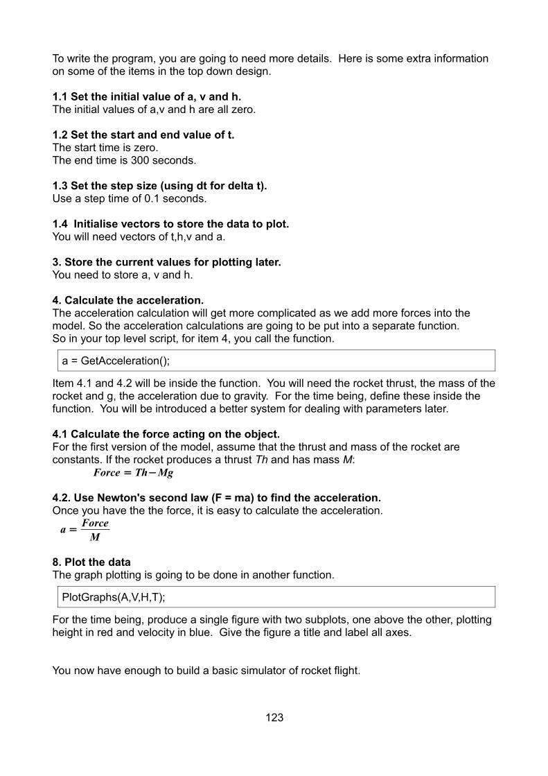
To write the program, you are going to need more details. Here is some extra information on some of the items in the top down design.

1.1 Set the initial value of a, v and h.The initial values of a,v and h are all zero.

1.2 Set the start and end value of t.The start time is zero.The end time is 300 seconds.

1.3 Set the step size (using dt for delta t).Use a step time of 0.1 seconds.

1.4 Initialise vectors to store the data to plot.You will need vectors of t,h,v and a.

3. Store the current values for plotting later.You need to store a, v and h.

4. Calculate the acceleration.The acceleration calculation will get more complicated as we add more forces into the model. So the acceleration calculations are going to be put into a separate function.So in your top level script, for item 4, you call the function.

Item 4.1 and 4.2 will be inside the function. You will need the rocket thrust, the mass of therocket and g, the acceleration due to gravity. For the time being, define these inside the function. You will be introduced a better system for dealing with parameters later. 4.1 Calculate the force acting on the object. For the first version of the model, assume that the thrust and mass of the rocket are constants. If the rocket produces a thrust Th and has mass M:

Force = Th−Mg

4.2. Use Newton's second law (F = ma) to find the acceleration. Once you have the the force, it is easy to calculate the acceleration.

a =ForceM

8. Plot the dataThe graph plotting is going to be done in another function.

For the time being, produce a single figure with two subplots, one above the other, plotting height in red and velocity in blue. Give the figure a title and label all axes.

You now have enough to build a basic simulator of rocket flight.

123

a = GetAcceleration();

PlotGraphs(A,V,H,T);

Exercise Set 3a Assuming constant thrust and constant mass and use the parameters in the table on page 120.

1. In an appropriate place in your home directory, create a directory called Rocket.Inside Rocket, create a directory called version1, for version1 of the rocket simulator.

2. Write a script, called rocket.m, using the top down design and notes on the previoustwo pages. Hint: Start by inserting the top down design as comments.

3. Write a function GetAcceleration(). Remember that the function has to be put in a file with the name GetAcceleration.m Hint: Again, use the top down design as comments.

4. Write the function PlotGraph.m.

5. Check that model is correct.Calculate the acceleration, using MATLAB as a calculator.

Use v=u+a t To calculate the velocity at 150 seconds.

Use s=u t +12a t 2 To calculate the hight after 150 seconds.

Check these values on the graph using the data cursor.

The expected output from exercise.

124

Increasing Simulation Complexity The code you have just written can be made more realistic by considering:

• A rocket's mass does not remain constant. The weight is reduced as the fuel is burnt off.

• After a time, it runs out of fuel.

• The faster a rocket moves, the greater the air resistance.

An analytic approach would be daunting, you could write down the differential equation butwould have no hope of solving it. However, the numerical approach using Euler's Method can very easily account for these. Begin by writing down the force balance on the rocket.

Force = Th+D−Mgwhere

Th is the thrust.M is the mass.D is the drag on the rocket.

Now just as before we can solve for the instantaneous acceleration:

a =ForceM

The acceleration at a time t must be some complicated function of time. This is no problemas you simply evaluate the numerical value of each of the terms on the right hand side at each step of the iteration.

The hard way of doing this is to try to do it all in one go. This makes it difficult to judge if the results produced by your model are reasonable. It also makes it easier to debug your code if you keep the size of any changes as small as possible. So there will be four new versions, each with their own design, build and test stages.

Exercise Set Version Incremental Change

3b 2 Variable Thrust

3c 3 Use Structures

3d 4 Variable Mass

3e 5 Include Drag

125

Exercise Set 3b In the first version, we assumed that the rocket thrust is always constant. However, we know that after the first stage of the rocket has burnt out, there will be no thrust. In this version we assume the thrust is constant during the burn period and zero after the burn period. We are only concerned with modelling stage 1 of the rocket. We could go on to model the other two stages later. The models should almost be identical, but with different starting parameters.

1. Create a new directory for version 2 of the program. The easiest way to do this is tocopy the directory for version 1. You can do this in a terminal window.

Or you can right click on a directory to copy and rename it in the left hand window inMATLAB.

2. Write a function called GetThrust. This function will be used to calculate the thrust of the rocket. The thrust will be constant for the whole of the burn time. After the burn time, all the fuel will have been burnt, so the thrust will be zero. The function will need the time as an input argument and it will return the thrust.

3. Use the function GetThrust in GetAcceleration to calculate the thrust. You will need to make time an input argument for GetAcceleration, so that it can be passed on to GetThrust. Test and debug your new code.

4. To see better what is happening, add a third subplot for the acceleration.

5. Check the graphs.◦ Use the data cursor to measure the acceleration before and after 150 seconds.

Is the acceleration graph what you would expect ?◦ Given the shape of the acceleration graph, do the velocity and height graphs

look reasonable?

This is a good point to step through your code, using the debugger. Place a break point inside rocket.m and use the Step and Step In icons.

What is the difference between the Step and the Step In ?What do you think Step Out does ?If you don't know, put the cursor on the icon and wait for a message to show.

Remember, within a function only local variables and parameters passed to the function are visible. Make sure you can reconcile what appears in the Workspace window with your understanding of functions and variables available within a function.

126

cp -r version1 version2

Organization of InformationYou probably found the last task required you to embed important magic numbers deep within your code. The burn time and the initial thrust are required inside GetThrust. This is always bad news. What if you wanted to simulate a different rocket or the second stage, you would have to remember to edit the GetThrust function. As the number of functions increases, it becomes harder to make changes. It also becomes easier to miss a particular magic number in one of the functions.

The standard is to define all such numbers in one location, at the top of your main program. However, then you have the problem of how to access them in your functions. You could supply more parameters to the function GetAcceleration, so that at run time you pass it all the parameters it could ever need. That is, something like

function acc=GetAcceleration(t,v,h,M0,MFinal,DragCoeff,Area, ...)

However, that soon starts to look cumbersome. You would have to repeat the same procedure for each function within GetAcceleration. In a large model, there could be over 100 parameters. Instead of making it easier, it starts to make it harder and more error prone.

Fortunately there is a better way. All the parameters can be stored together into a structure. A structure is a group of variables with a single variable name. They are very easy to create. Type the following into the command window.

You have created a structure called S. It has three fields called n, v and name. Each fieldcan hold anything that you can put into a conventional variable. So S is like a bag that contains three other variables.

You can treat S as a single entity or you can access the individual fields.

Try creating your own structure using your own field names. Copy the new structure to another variable. Then try displaying the individual fields from the copy of your structure.

127

>> S.n = 42>> S.v = [1,2,3,4]>> S.name = 'John'

>> S>> S.n >> S.v >> U = S>> U.name

Exercise Set 3c1. Create a new version.

2. Add the following to the top of rocket.m

3. Pass Mdata as an argument to GetAcceleration.

Rewrite GetAcceleration so that the value of g is obtained from the argument Mdata.

Or you can substitute Mdata.g into your calculations. Check that the program still works.

4. Edit both GetAcceleration and GetThrust so that no constants (magic numbers) appear anywhere apart from at the top of rocket.m

5. Modify your code and relevant functions by introducing a state structure which will contain a snap-shot of time varying properties of the rocket. Such as the current mission time, velocity and height. So instead of passing t ; v ; h around you'll pass asingle structure which contains these fields.

128

% Model ParametersMdata.initialMass = 2.9e6; % kgMdata.initialFuelMass = 2.15e6; % kgMdata.burnTime = 150; % SecondsMdata.initialThrust = 34e6; % NewtonsMdata.dragConstant = 0.6; % Ns ^2 m^-2Mdata.g = 9.81; % Acceleration due to gravity m/s^2

a = GetAcceleration(t,Mdata);

g = Mdata.g;

state.t = t; state.h = h; state.v = v; % store state variablesa = GetAcceleration(state,Mdata); % get acceleration

Exercise Set 3d Almost 75% of the initial mass of the rocket is the fuel for the first stage. So there will be aconsiderable mass reduction as this fuel is burnt off, in the first 150 seconds. This needs to be taken into consideration to obtain a reasonable model of the rockets performance.

So in this version, we are going to assume that there is a linear reduction in the rocket mass, while the fuel is being burnt. Then the mass will be constant, after all the fuel has gone. Please note that the initial mass of the rocket given in the table on page 120 includes the mass of the fuel.

1. Create a new version.

2. Add two more model parameters to Mdata in the top of rocket.burnRate The rate at which the fuel is used in kg/s.finalMass The rocket mass without the fuel.

Add these two parameters to the end of the model parameters block at the top of rocket. The values must be calculated in the program, using the model parameters already available.

3. Write a function called GetMass. This function will be used to calculate the mass of the rocket as the fuel is burnt off. The burn rate will be constant for the whole of theburn time. After the burn time, the mass will be constant. The function will return the mass.

4. Use the function GetMass in GetAcceleration to calculate the mass. Test and debug your new code.

5. To see what is happening, add a fourth subplot for the mass of the rocket.At the moment, the mass does not exist in the top level of the program. How are you going to obtain a vector of the rocket mass so that it can be plotted ?

129

Exercise Set 3e We are going to use a very simple model for drag. The resistance is proportional to the square of the velocity and is always opposite to the direction of the velocity.

drag=−k v2

The drag constant k you should find in the model parameters that you entered earlier. In reality, the constant will get smaller as the rocket gets higher and the air gets thinner. This could be included in future models.

The above equation is not entirely correct. What happens if the velocity is negative, will the drag still be in the opposite direction to the velocity?

Is the following any better ? drag=−k v∣v∣

1. In a new version, write a function called GetDrag to calculate the drag. Use this function in GetAcceleration.

2. In PlotGraph, use the max function to find the maximum acceleration and the time when it occurs. Then use the text function to write “maximum acceleration” on the acceleration graph at the appropriate place.

3. Use the sprintf function to include the actual value of maximum acceleration in the text written on the acceleration graph.

4. Repeat the above for the minimum acceleration.

5. Is the drag function working correctly? When there is no fuel, what would the acceleration would be if there was no drag. Look at the velocity graph and then think about the difference the drag is making to the acceleration.

6. Change the model so you can observe the graphs 400 seconds after take off. Use the data cursor to find the point where the velocity goes negative. Make a note of the time the velocity goes negative. Use the data cursor to find the same point on the acceleration graph and the height graph. What do you notice ? Is this what youwould expect ?

7. Try runs with different drag coefficients.

AssessmentGet a demonstrator to look at your programs, how they work and your programming style. This will give you a valuable insight into how you will be assessed at the end of session 5.

This is not a formal assessment. There are no marks for session 3.

130

Practice 2

This practice activity is for you to test your ability to design programs before session 4. This is just for fun. So if you get stuck or find it too challenging, do not worry.

The solutions programs can be download from the course web site. Please do look through the solutions. They will help you understand how to lay out your own programs in the final two session.

Practice ActivityThere are two gliders on an air track connected together by a spring.

The gliders can only move backwards and forwards in the x direction. As there is no friction between the gliders and the air track, the only force on the gliders is from the spring.

Force onGlider1 = F1 = ( x2− x1−nl )k

Force onGlider2 = F 2=−F 1

Where nl is the natural length of the spring

and k is the spring constant.

PTO

131

Glider 1 Glider 2

xx2

x1

Top Down Design

Write a top down design for a program to plot the position of the two gliders using Euler's Method.

HintYou can cut down on the amount of work required by using arrays to hold the information about the gliders. For example, you could use Euler's Method to find the position of each glider separately.

x1= x1+ v1dt

x2= x2 + v 2dt

or you could do both the above with one line.

x = x + v dt Where x = [ x1x 2] and v = [v1v2]This also makes it easier to modify the program to simulate systems with more gliders.

132

Version 1

Write a MATLAB program using the top down design.

Usingm1= m2 = 0.1 kg The mass of the gliders.

k = 0.1 N /m The spring constant.

nl = 0.1 metres The natural length of the spring

x1 = 0.1 metres The initial position of glider 1

x2 = 0.2 metres The initial position of glider 2

v1 =−0.05 m / s The initial velocity of glider 1

v2 = 0 m / s The initial velocity of glider 2

tstart = 0 seconds The start time

tstop= 20 seconds The stop time

dt = 0.001 seconds The step size

• Put the code to plot the graph into a function. Plot both x1 and x2 in red on the same graph. Also plot the average of x1 and x2 in blue.

• The average of x1 and x2 is the centre of mass of the system. As there are no external forces on the system, the centre of mass should obey Newton's first law and move with a constant velocity.

• One thousand steps a second may seem like an excessively small step size. However, if you have a larger step size, the error in the model makes the oscillations of the system grow. To see this, try setting dt to 0.02 and 0.1.

133

Version 2

Now assume that there is buffer at x = 0 to stop the glider from coming of the end of the airtrack. Change the program to simulate what happens after the glider hits the buffer.

You can simulate a buffer at the end of the air track by changing the program so that both x1 and v1 are set to zero when x1 goes negative.

Change the initial conditions so thatv1 =−0.05 m / s The initial velocity of glider 1

v2 =−0.05 m /s The initial velocity of glider 2

134

Version 3 Animation

The previous version produced an array of data to plot a graph. Instead of using this data to plot a graph, use it to produce an animation of the motion of the gliders.

• You can use the functions drawshape, fillshape and translate from the exercises at the end of session 2.

• You can represent the gliders by a simple oblong block.

• If you want to animate the spring, the following script shows you how.

• With 1000 steps per second, the animation is going to be very slow. To speed things up you can use decimation. Only using every tenth step or every seventh step or every nth step. As an example, change n in the program above to 2500.Then run the program. It will be 5 times slower.

Now change the for loop so that only every 5th step is animated.

The speed will be similar to the original program.

When you have the program working, play around with different initial conditions.

135

%Demonstrate how to animate the spring. n = 500; % the number of framest = linspace(0,6*pi,n);X = 2 + sin(t); % Define the shape of the springspring = [ 0:0.1:1 ;-0.5 0.5 -0.5 0.5 -0.5 0.5 -0.5 0.5 -0.5 0.5 -0.5]; %Repeat for every framefor k = 1:n x = X(k); sp2 = [x 0; 0 1] * spring; % Stretch the spring by x drawshape(sp2,'k'); % Display the spring axis([0,5,-1,1]) axis('equal') drawnowend

for k = 1:5:n

There is a video on the web of two gliders on an air track connected by a spring.

http://techtv.mit.edu/videos/674-push-me-pull-you

Or search in google for Air track push me pull you.

If you want to do more

There are lots of things you can do to extend the model. If you want to

• Simulate a second buffer at the other end of the air track.

• Simulate three or more gliders connected by springs.

• Simulate what happens if the air track is slopping, so that gravity has to be taken into account.

136

Session 4 & 5

DBT Part B: The Lander Controller

Introduction

The second part of the Computing Design Build and Test is more open-ended, and you will have to make your own decisions and then implement them.

The picture on the right shows the Phoenix Lander about to make touch down on the surface of Mars. In this part of the DBT, you will be designing the software to safely land a vehicle such as this on the surface of a planetor moon.

The problem shares many of the features of the Saturn V launcher in Part A. The difference is that the amount of thrust at any time is crucial.If not enough thrust is used, the lander will hit the surface at high speed and wreck the vehicle. If too much thrust is used, the lander will start going up.

A control system will be used to set the amount of rocket thrust. The problem is to design a control system to get the lander safely to the surface of a planet or moon.

The controller will repeatedly inspect the height and velocity and calculates a sensible thrust to be generated by the rocket motor.

137

ControllerRocketMotor

Thrust

Computer

Height

Instrumentation

Velocity

Obviously, testing the controller using a real rocket and lander is just not practical. So you will also need to design a lander simulator.

The lander simulator will use a dynamic model to predict how the lander will behave. The simulator will use the same methods as used in the rocket simulator in Part A

138

Controller Simulator

Thrust

Velocity

Height

Example, A Ball Thrown UpwardsBefore starting the lander exercises, we are going to look back at the program to model the ball being thrown into the air. The approach taken here is slightly different to the modelused in session 3. This new version has more of the features that will be required for the Lander Simulator exercises.

The top down design of the program is

Using Euler's Method to Plot a Ball Thrown Upwards.

1. Initialise the values.

1.1 Set the Model Parameters.

1.2 Initialise vectors to store the data to plot.

2. Repeat for each time step while above the ground.

3. Store the current values of both h and v for plotting later.

4. Run the simulator to predict what will happen over the next time step.

4.1 Use Euler's method to find the position at the next step.

4.2 Use Euler's method to find the velocity at the next step.

4.3 Increase the time by dt.

5. End of repeat.

6. Plot the data.

The program looks like thisball2.m

139

%Using Euler's Method to Plot a Ball Thrown Upwards. %1. Initialise the values%1.1 set the Model Parametersstate.a = -9.81; % Acceleration m/s^2state.dt = 0.01; % The step size in secondsstate.v = 25; % The initial velocity m/sstate.h = 1e-9; % The initial height meters. Must be >0 to start.state.t = 0; % Start time in seconds % 1.2 Initialise vectors to store the data to plotn = 600; % The total number of pointV = zeros(1,n); % Vector to store the values of v.H = zeros(1,n); % Vector to store the values of h.T = zeros(1,n); % Vector to store the values of t. k = 0; % the step counter

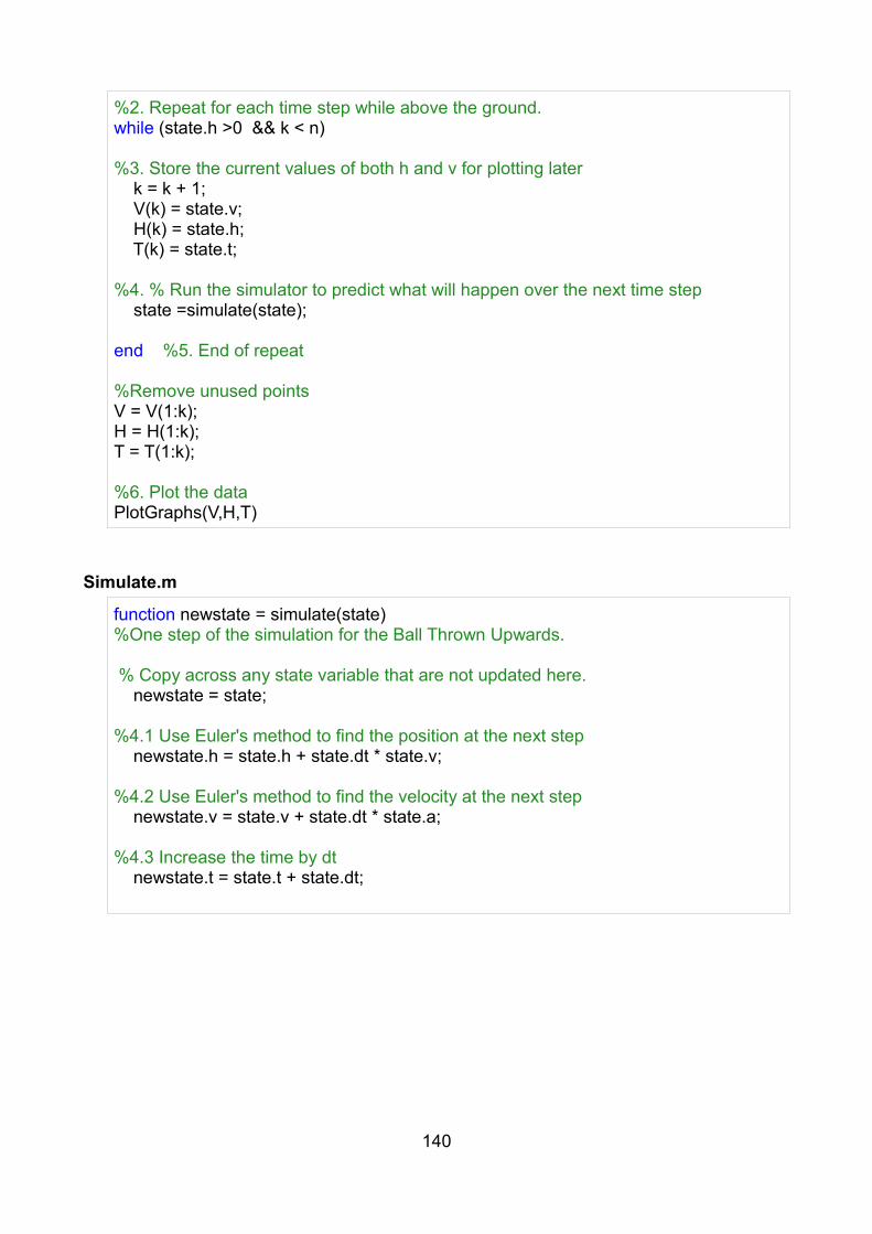
Simulate.m

140

%2. Repeat for each time step while above the ground.while (state.h >0 && k < n) %3. Store the current values of both h and v for plotting later k = k + 1; V(k) = state.v; H(k) = state.h; T(k) = state.t; %4. % Run the simulator to predict what will happen over the next time step state =simulate(state); end %5. End of repeat %Remove unused pointsV = V(1:k);H = H(1:k);T = T(1:k); %6. Plot the dataPlotGraphs(V,H,T)

function newstate = simulate(state)%One step of the simulation for the Ball Thrown Upwards. % Copy across any state variable that are not updated here. newstate = state; %4.1 Use Euler's method to find the position at the next step newstate.h = state.h + state.dt * state.v; %4.2 Use Euler's method to find the velocity at the next step newstate.v = state.v + state.dt * state.a; %4.3 Increase the time by dt newstate.t = state.t + state.dt;

Copy the code into the appropriate files and write your own PlotGraphs function.

Then run ball2.

Question 1

Why can we not set the initial value of h to zero?

Question 2

The purpose of the code after the while loop is to remove unused points. What would happen if this code is commented out?

Question 3

Why is there a test for k<n in the while loop?

What would happen if we changed this to

Question 4

Increase the initial velocity to 30 m/s. Why does the program stop before the ball hits the ground? What can you do to correct this?

Warning

Before starting the final project, read through How to get good marks on page 121 again.If you do not follow of the advise on page 121, YOU WILL LOSE MARKS.

141

while (state.h >0 && k < n)

while (state.h >0 )

The Lander Simulator and ControllerWe now return to the problem of simulating and controlling a planetary lander. Read through the description of the problem on this and the next page, then start on the exercises on page 137.

The top level program design will look something like this.

The lander simulator and controller

1. Initialise the values.

1.1 Set the Model Parameters.

1.2 Initialise vectors to store the data to plot.

2. Repeat for each time step while above the ground.

3. Store the data to plot later.

4. Get the thrust from the controller.

5. Run the simulator to predict what will happen over the next time step.

5.1 Calculate the acceleration.

5.1.1 Calculate the total mass.

5.1.2 Calculate the force.

5.1.3 Use Newton's second law to calculate the acceleration.

5.2 Use Euler's method to find the position at the next step.

5.3 Use Euler's method to find the velocity at the next step.

5.4 Increase the time by dt.

6. End of repeat.

7. Plot the data.

I hope that you can see that steps 5, 5.1 and 7 are going to require a lot more code. These are going to be functions.

You can test a simulator without a controller, but you cannot test the controller without a simulator. So the first versions of the program are going to concentrate on designing the simulator. For the very first version we are going to keep things as simple as possible. Assume that the only force is gravity. There will be no drag or thrust.

142

Top Level Design Details

You will need more detail for some of the steps in the top level of the program.

1. Initialise the model variablesWe are going to use structures to make it easier to pass the data to the functions.

4. Get the thrust from the controllerJust set the thrust to zero for now:-

5. Run the simulator to predict what will happen over the next time stepThe first few versions are going to develop a simple simulator. In many ways, the simulator is very like the Saturn V rocket simulator is session 3. The simulator function is going to be called simulator(). It takes a copy of the structure state and returns a new version of state containing all the updated variables.

Hint: See the previous example

3. Store the data to plot later and 6. Plot the dataUse the same method as in the previous example.

5.1 Calculate the AccelerationThis is going to be a function called GetAcceleration(). The function will need the state and the thrust. It will return the acceleration.

Have a look back at GetAcceleration(), used in session 3 for more guidance. In the first version, the only force acting on the lander will be gravity. This function is going to get more complex in later versions when we start to bring in other forces.

143

thrust = 0;

% Initialise Lander structurestate.fixedmass = 500; % kg Mass with no fuelstate.fuelmass = 1500; % kg state.g = 9.81; % Acceleration due to gravity m s^-2state.a = -state.g; % Acceleration m s^-2state.v = -300; % Velocity m /sstate.h = 3000; % Height mstate.t = 0; % Time sstate.dt = 0.1; % Step size s

state = simulator(thrust,state);

Building the simulator: Exercise Set 4a

1. Produce the first version of the Lander program using the model on the previous pages. To start with, assume that there is no thrust or drag and that the mass is constant. Plot the height, velocity, acceleration and fuel mass against time.

2. The model so far has constant acceleration. So you can use the constant acceleration equations to check that the model is working. In the MATLAB command window use

v2=u2+2a s To calculate the velocity when the lander hits the ground.

s=12(v+u) t To calculate the time when the lander hits the ground.

Compare these values with those obtained from the graphs. Click on the Data Cursor icon on the figure, then click on a point on the graph to displayvalues of the graph at that point. You can drag along the graph to the pointwhere the lander crashes.

3. Create a second version of the program with non zero, constant thrust. Test the model with different values of thrust.

For large values of thrust, the Lander will go upwards forever. So the program may never end. To stop the program, click in the command window, hold down the Ctrl key and press the C key.

Hint: This is the last time that you will be told to create a new version. From now on you decide when to create a new version.

4. At the moment the mass of the Lander is a constant 2000 kg. In the command window, calculate the weight of the Lander. Set the thrust equal to the weight of theLander. Check the behaviour of the model is what you would expect.

5. In the real world, the rocket will run out of fuel after a period of constant thrust. Alsothe weight of the fuel is a large portion of the total weight of the Lander. So the dynamics of the Lander will change considerably as the fuel is used. The Lander consumes fuel at a rate of 0.001 kg per Newton of thrust per second. Change the function simulator() so that when the Lander has fuel, the new fuel mass is calculated.

When there is no fuel, what should the thrust be set to ?

Hint: Is it possible for the fuel mass to be negative in your model? What should happen if the fuel mass is negative? If the thrust is negative, would you expect the fuel mass to increase ?

144

6. It is important to test the model works with and without fuel. To do this, set the thrust to a large value(say 50000 Newtons) so that the Lander goes up. Are the graphs what you would expect?

7. At what time does the fuel run out ?Calculate the time by hand and compare with the time on your graph.

8. Find the peak height and calculate the potential energy.Potential Energy= m g h

Find the velocity at impact and calculate the kinetic energy.

KineticEnergy =12mv2

Are the results consistent with what you would expect?

9. The final part of the simulator development is to add drag. Use the following equation to write a drag function.

drag=−∣v∣v3

where v is the velocity of the Lander.

10.Test the model with drag and a constant thrust of 50000 Newtons. How does the acceleration change at the peak height?

11. Calculate the terminal velocity of the Lander without fuel. This occurs when the drag is equal to the weight of the lander.

drag =v2

3=mg

Terminal Velocity = v = √3m g

As the Lander approaches its terminal velocity, drag will cancel out the force of gravity and the acceleration will reduce to zero. Is this consistent with what happens in your simulation?

12.Can you explain the large change in acceleration when the fuel runs out ?

145

The ControllerControl is an important area in Information Engineering. You start learning about this seriously next year. Before moving on to the next set of exercises, you need to understand some of the principles of control theory.

The overall objective of the controller is a gentle touch down on the ground. In theory, if everything was known ahead of time, you could write a differential equation and solve it in advance. However, in practise this does not work. There are always uncertainties due to unmodelled and unpredictable disturbances, such as a sudden down draught in the atmosphere or a slight difference between the actual and calculated thrust. You need to beable to recompute the required thrust from moment to moment.

This is where automatic control comes in. A control system compares a process output with what you desire it to be. It then alters the input into the system to correct the error.

The diagram below illustrates the idea.

In a real system, the controller is most likely to be a piece of software running on a computer, but the process being controlled (the rocket vehicle) is the physical mechanism itself. The outputs from the process are measured using sensors (altimeters, radar, star fixes, etc). Later in the course, you get to control real mechanisms, but here you have to simulate the behaviour of the mechanism. In case this seems disappointing, it is what happens in “real” engineering design too.

146

ControllerOutput

ProcessErrorDesired

Output -+

Control System

Negative Feedback

We are going to be using a very simple type of controller called a proportional controller.

Here x represents the desired output and y the actual output. So the error e is

e = x − y

A proportional controller simply multiplies the error by a constant k.

u= k e

To simplify things even more, I have represented the process to be controlled by a function.

y = f (u)

f −1( y) = u Where f −1( y) is the inverse of f (u)

f −1( y) = k e

f −1( y )k

= e

So if k is very large, the error e will be small.

Although the above gives you an idea of how a proportional controller works, in practice the process is more complicated than a simple function. There is normally a delay while the process adjusts to the new input. For example, you control the speed of a bus using the accelerator pedal. It takes time for the bus to get to the desired speed.

A large value of k may not be desirable. In the case of the bus, high acceleration would make the passengers uncomfortable. In the case of the lander, this will produce very largeamounts of thrust for a very small error. The acceleration rate will be huge. This could damage the instrumentation, or kill the occupants if it is a manned mission.

147

yf(u)

uex -+

Proportional Control

Negative Feedback

k

We wanted the lander to descend at some desired velocity, lets call it vd . The simplest thing we could do would be to set the rocket thrust to be proportional to the difference between our actual velocity v and our desired velocity vd.

Error = vd − v ; thrust = k × ErrorWhere k is a suitably chosen “gain” constant to be found by experiment.

There is a built in MATLAB function called “error”, so avoid using this as a variable name. Built in MATLAB function names nearly all use lower case letters, the variable name “Error” is fine. There is one slight problem here: when the velocity is correct ( vd = v ) the engine generates no thrust, but the vehicle is still accelerating under gravity. So although the lander velocity matches the desired velocity exactly, the Lander will still accelerate due to gravity. The controller will automatically adjust to compensate for gravity, but this will produce a large error. In other words, the control system needs a large error to generate the thrust required to overcome gravity. You could compensate for this by making k very large. However, as mentioned earlier, very large k is not always desirable.

In exercise set 4A, question 4, you set the thrust equal to the weight of the Lander. This cancelled out the acceleration due to gravity. The controller can use the same principle. We will assume that it is able to measure or calculate the mass of the Lander and calculate the thrust required to overcome gravity. This can then be added to the output of the proportional controller.

Error = vd − v ; thrust = k × Error + mg

If the error is now zero, the controller will generate enough thrust to overcome gravity, so the error should stay at zero.

148

Velocity vSimulator

ThrustErrorDesiredVelocity

vd

-+

Proportional Control

Negative Feedback

k

Thrust = k×Error

Velocity vSimulator

ThrustErrorDesiredVelocity

vd

-+

Negative Feedback

k

Thrust = k×Error + mg

++

mg

Remembering that the controller could be required to work with the real system and not with a simulator, it is desirable to keep the control parameters in their own separate structure.

149

%Initialise Controller structurectrl.vdesired = 0; % m/s Hover to start with ctrl.gain = 1000; % A guess to start with

Building the Controller: Exercise Set 4b

1. Write a function called Controller() which makes the vehicle hover at some positive height (but don't specify the height yet). When the vehicle runs out of fuel it should crash. To get started, make the controller gain k 1000.

2. You'll need to play around with your choice of the controller gain k . To avoid damaging any occupants of a manned lander, we need to keep the acceleration to under 6g.

• What is the maximum acceleration attained by your Lander model ?

• Why does the maximum acceleration occur where it does ?

• Reduce the value of k to see what happens to the maximum acceleration.

3. As you reduce k, it takes longer for the controller to get the lander under control. The height at which the lander hovers becomes lower and lower. If k is too small, the lander will hit the ground before the controller can bring it under control.

The landing struts on the Apollo Lunar Module could withstand no more than 2 m/s. Try to adjust the the value of k so that the lander hits the ground at less than 2 m/s.Is reducing the ability of the controller to bring the lander under control in this way a good thing to do?

4. The way to answer the above question is to stress test the model.

• Test the model with a initial velocity of -290 and -310 m/s.

• Try changing the initial height to 3100 and then to 2900 metres.

I hope that you can see that the controller has lost the ability to compensate for small changes. As you work through the remainder of this laboratory, you must stress test your models. The whole point of having a controller is that it can compensate for small changes and disturbances. The above test will be part of the assessment of your program.

150

5. Try setting the desired velocity to -2 m/s and k = 500.You should find that the descent takes too long. The lander runs out of fuel long before touchdown. You could reduce k, but then you get the same problem as above. I hope that by now you are convinced that trying to maintain a constant desired velocity is not going to work.

6. Although the model with small k was not very resilient, it does point the way to a better model. Reducing the value of k allowed the lander to maintain a higher speed for longer. This meant it took less time to reach the ground. So it did not runout of fuel. Instead of achieving this by destroying the ability of the controller to maintain a speed, the desired velocity needs to be larger when the lander is high up. The desired velocity needs to be a function of height. The lander needs to descend faster when it is high up, and slow to less than 2 m/s as it gets near to the ground.

Assume that the desired velocity is a linear function of height.

• What do you think the desired velocity should be at touch down and at a height of 3000m ?

• Sketch a graph of desired velocity against height.

• What is the slope and the intercept ?

Change Controller() so that the desired velocity is dependent on the height.You will probably have to increase the controller gain k .

7. Annotate the graphs so that the values of maximum acceleration, the landing velocity and the fuel mass remaining at touch down are shown.

151

8. Now see if you can find a way of getting down safely using less fuel. Here are some ideas you may want to consider :

• Different values of controller gain k.

• Use a different function for the desired velocity.

• Let the Lander drop for longer before bringing it under control.

• Limiting the maximum thrust to prevent large amount of acceleration.

• Stopping the controller from producing negative thrust.

Compare the results with the linear model produced for question 6.None of the above are guaranteed to improve your model.

You do not have to try all the above suggestions in question 8. Try coming up with your own ideas. What you do is your choice.

Please keep a working version of everything you try. A good idea that has been well modelled and tested can get good marks, even if the result is not as good as the linear model.

AssessmentBy early afternoon of your final session you should be ready to be assessed. Before being assessed, read through How to get good marks on page 121 and make sure you that you are not going to lose marks.

In the final assessment you demonstrate your working code. You will need to show :

• The simulator and controller working together, driven by a top level script or function, to bring the vehicle to a smooth landing.

• That your model can withstand the stress test in question 4.

• Graphs which show the vehicle landing. The demonstrator will need to know the landing velocity, the maximum acceleration and the amount of fuel remaining.

• Evidence that this is your own work. Explain your program, particularly what you didfor question 8.

152