Ozone ﬂ ux measurements over a Scots pine forest using eddy covariance method ... ·...

BOREAL ENVIRONMENT RESEARCH 8: 425–443 ISSN 1239-6095Helsinki 10 December 2003 © 2003

Ozone fl ux measurements over a Scots pine forest using eddy covariance method: performance evaluation and comparison with fl ux-profi le method

Petri Keronen1), Anni Reissell1)2)3), Üllar Rannik1), Toivo Pohja4), Erkki Siivola1), Veijo Hiltunen1), Pertti Hari4), Markku Kulmala1) and Timo Vesala1)

1) University of Helsinki, Department of Physical Sciences, P.O. Box 64, FIN-00014 University of Helsinki, Finland

2) University of Helsinki, Department of Chemistry, P.O. Box 55, FIN-00014 University of Helsinki, Finland

3) Finnish Meteorological Institute, Air Quality Research, Sahaajankatu 22 E, FIN-00880 Helsinki, Finland

4) University of Helsinki, Department of Forest Ecology, P.O. Box 27, FIN-00014 University of Helsinki, Finland

Keronen, P., Reissell, A., Rannik, Ü., Pohja, T., Siivola, E., Hiltunen, V., Hari, P., Kulmala, M. & Vesala, T. 2003: Ozone fl ux measurements over a Scots pine forest using eddy covariance method: performance evaluation and comparison with fl ux-profi le method. Boreal Env. Res. 8: 425–443. ISSN 1239-6095

Ozone fl uxes were measured over a forest in southern Finland between August 2001 and July 2002 using the eddy covariance method. Systematic errors due to the imper-fect frequency response of the instrumentation and random errors due to the stochastic nature of turbulence were estimated. Flux underestimation correction factors for unsta-ble stratifi cation were 1.03–1.19. Random errors of the fl ux estimates were most fre-quently about 20% of the fl ux value. Fluxes were highest during the summer, declining to near zero during the winter. In summer, fl uxes were higher during daytime than at night coinciding with higher turbulence and higher rate of stomatal uptake. Maximum summertime deposition velocities were 6–7 mm s–1. During winter, the diurnal pattern in ozone fl ux was weak and the deposition velocity was 0.5–1.5 mm s–1. Comparison between eddy covariance and profi le fl ux measurement results generally showed good agreement during daytime.

426 Keronen et al. • BOREAL ENV. RES. Vol. 8

Introduction

In order to understand the transfer of ozone (O

3) between the atmosphere and vegetation,

atmospheric chemistry, meteorology, transport and vegetation uptake mechanisms need to be considered. That is, several processes affect the ambient air mixing ratios of ozone, as well as fl uxes and deposition velocities. Ambient air mixing ratios depend on transport, local for-mation and destruction in photochemical and other reactions, and on the volume and mixing conditions of the boundary layer. Uptake by vegetation through stomata is considered to be a large sink for surface ozone, and therefore the factors affecting the opening and closing of stomata (light, temperature, humidity, wetness, water availability) have often been examined (e.g. Meyers et al. 1998, Wesely and Hicks 2000). However, recent studies provide evidence that non-stomatal routes for O

3 deposition may

account for a considerable portion of the total uptake by a forest ecosystem (e.g. Zeller and Nikolov 2000, Lamaud et al. 2002).

Several techniques have been used to meas-ure fl uxes of chemical species between the atmosphere and the surface (Wesely et al. 1989, Dabberdt et al. 1993, Zeller 1993, Rinne et al. 2001, Altimir et al. 2002, Guenther 2002). Aero-dynamic (or micro-meteorological) methods rely on measuring the vertical concentration profi le (profi le method), the concentration difference between up- and downward directed air-drafts (eddy accumulation and relaxed eddy accumula-tion methods) or the concurrent turbulent fl uc-tuations of vertical wind speed and concentration (eddy covariance and disjunct eddy covariance methods). In the profi le and accumulation meth-ods fl ux-profi le and fl ux-concentration difference relationships are needed to calculate the fl uxes. In the eddy covariance (EC) methods the fl ux is obtained directly from the covariance between the wind speed and concentration data. Non-aerodynamic methods determine the change of concentration in an enclosure or measure the mass deposited on or evaporated from a natural or a surrogate surface.

Aerodynamic methods require relatively large uniform fl ux source areas, stationary atmospheric conditions and fl at topography. On the other

hand, these methods are more representative in a larger scale than non-aerodynamic methods, since they can be used to quantify the average vertical fl ux over several hundred square meters extending both upwind and crosswind from the measurement point.

The profi le technique requires accurate meas-urements of concentration differences. With the eddy accumulation, relaxed eddy accumulation and disjunct eddy covariance techniques rela-tively slow sensors can be used (Wesely et al. 1989, Rinne et al. 2001). The eddy covariance technique requires measurements of very rapid turbulent fl uctuations and therefore the used sen-sors and analysers should have a short response time combined with a high selectivity. The eddy covariance technique is considered as a reliable measurement method for turbulent exchanges of momentum and heat in the atmosphere. It is also suitable for fl ux measurements in the vicinity of uneven terrain, such as hills, and in slightly non-stationary situations (McMillen 1988), and it is the only method suitable for fl ux measurements inside forest canopies (Arya 2001).

Ozone fl ux measurements over Scots pine (Pinus sylvestris L.) forests are scarce (Rondon et al. 1993, Aurela et al. 1996, Tuovinen et al. 2001) but fl uxes over other coniferous trees encountered in the northern boreal region, such as the Norway spruce (Picea abies), have been reported (Pilegaard et al. 1995, Mikkelsen et al. 2000). Duyzer et al. (1995) reported ozone fl ux measurements above Douglas fi r. Suni et al. (2003) compared ozone fl ux results with fl uxes for CO

2, latent heat, and particles. Pos-

sible sources of errors in micrometeorological techniques have been reported (Businger 1986, Wesely et al. 1989, Kaimal and Finnigan 1994, Lenschow et al. 1994, Foken and Wichura 1996), but few publications have actually presented an error analysis (Businger 1986, Rannik 1998a, Finkelstein and Sims 2001) or compared the dif-ferent fl ux measurements methods (Zeller 1993, Guenther et al. 1996, Mikkelsen et al. 2000).

In this paper, we present ozone fl ux results obtained by eddy covariance method. This study covers the measurement period from August 2001 to July 2002. To our knowledge, no winter-time ozone fl ux or deposition velocity data over Scots pine forests have previously been reported.

BOREAL ENV. RES. Vol. 8 • Ozone fl ux measurements over a Scots pine forest 427

We describe the eddy covariance measurement system, estimate the magnitude of systematic and random errors, and compare the eddy cov-ariance fl ux results with results from profi le fl ux measurements. The diurnal and seasonal varia-tions of ozone fl ux and deposition velocity are discussed. The ozone concentration profi les are also discussed in relation to turbulence.

Experimental

Site description and infrastructure

The SMEAR II measurement site (Station for Measuring Forest Ecosystem–Atmosphere Rela-tions) at the Hyytiälä Forestry Field Station of the University of Helsinki is located in south-ern Finland, 220 km northwest from Helsinki. The measurement station (61°51´N, 24°17´E, 181 m above sea level) was established in July 1995 and the continuous measurements started in January 1996. The forest stand surrounding the SMEAR II station was established in 1962 by sowing and the most homogeneous area is predominantly Scots pine with other species accounting for only 1% of the stand. The homo-geneous area extends approximately 200 m in all directions and the mean height of the domi-nant trees in the stand is 14 m. A more detailed description of the site is given in Rannik et al.

(2002). The site has been evaluated to be suit-able for micrometeorological fl ux measurements in unstable or near-neutral conditions (Rannik 1998b). The site is located in a background area, but a nearby source of pollution is the Forestry station building complex approximately 600 m to the southwest of the site. About 10 km to the southeast, two possible sources of regional pol-lution are a saw mill and local power plant in the village of Korkeakoski. About 60 km west to southwest from the station is Tampere, a city of about 200 000 inhabitants.

Eddy covariance measurements of momen-tum (t), sensible heat (H ), carbon dioxide (CO

2),

latent heat (LE) and ozone fl uxes were carried out at 23-m height, approximately 10 m above the top of the canopy, by means of a low tower (height 18 m) equipped with an extension rod (Fig. 1). Measurements of solar radiation were carried out also in this low tower. O

3 profi le

measurements were performed at six heights (67.2, 50.4, 33.6, 16.8, 8.4 and 4.2 m) in a high tower (height 73 m). The horizontal separation between the low tower and the high tower is about 25 m. Eddy covariance measurements of momentum, sensible heat, CO

2, latent heat and

aerosol particle fl uxes were carried out also in the high tower (at the height 23 m). More information on the infrastructure of the station is given in Vesala et al. (1998) and Kulmala et al. (2001).

Fig. 1. The measurement towers and instrumenta-tion set-up at the SMEAR II site in Hyytiälä.


Eddy covariance method

Turbulent fl ux may be considered as a superpo-sition of eddies of different sizes (frequencies). Generally the vertical mass fl ux of a substance (F

c) is given as the time average of the product

of the con-current vertical wind velocity (w) and concentration of the substance (c) (e.g. Arya 2001). The instantaneous values of w and c can be decomposed into a mean and a fl uctuating component (so called Reynolds decomposition). The fl ux of the substance is thus

(1)

The over-bars denote the time average and the primes the fl uctuating part. The time aver-ages of the fl uctuating components (w´ and c´) are zero.

With eddy covariance method the fl ux (Eq. 1) at the measurement height is obtained as a direct result. The frequently used formulation for dry deposition assumes that the deposition fl ux is directly proportional to the local concentration at the measurement height

F = –vdc (2)

where F is the fl ux, c is the concentration at the measurement height and v

d is a proportional-

ity constant known as deposition velocity (e.g. Seinfeld and Pandis 1998). By convention a fl ux downwards has a negative sign, giving a positive deposition velocity (Eq. 2) for a depositing sub-stance. The deposition velocity gives an indica-tion of the combined magnitude of all the physi-cal, chemical and physiological processes caus-ing the fl uxes regardless of the concentration.

There are several requirements that should be met when applying the eddy covariance method (McMillen 1988, Kaimal and Finnigan 1994, Foken and Wichura 1996). A common assumption is that the mean vertical wind speed is zero. If the area around the measurement point is fl at, this assumption holds suffi ciently well even though the wind speed is strictly not zero. The deviation from zero is however very small. The eddy covariance method can, however, be applied also in a sloping terrain, because it allows mathematically to force the vertical wind

speed to zero by coordinate rotations, that is by rotating the mean wind vector to local stream-lines. The time series should also be stationary during the measurement period, but eddy cov-ariance method can also be applied in slightly non-stationary conditions (McMillen 1988). Furthermore, for the measured fl ux to represent the surface fl ux around the measurement site, a horizontal homogeneity is required within the fl ux measurement source area. The eddy covari-ance method requires fast measurements of wind speed and concentration. Ideally, the frequency response of the sensors and analyzers should be at least 10 Hz (Wesely et al. 1989, Kaimal and Finnigan 1994). Measurement resolution for wind speed and temperature should be at least ±0.05 m s–1 and 0.05 °C, respectively (Kaimal and Finnigan 1994), and the measurement reso-lution of the concentration should give a signal-to-noise ratio of at least 30 (Wesely et al. 1989). When using a tower to reach the layer above a canopy, the sensors should be at least three lat-eral dimensions above the top of the tower and supported by a thinner mast or rod (Kaimal and Finnigan 1994).

Measurements

Wind speed and air temperature

An acoustic anemometer (Solent Research HS1199 ultrasonic anemometer, Gill Ltd., Lym-ington, Hampshire, England) has been installed at a height of 23 m by means of an 18-m-high tower (dimensions 2 ¥ 3 m) and 6-m-long rect-angular (dimensions 50 ¥ 50 mm) extension rod. Above 16 m the tower is relatively unobstructed with a ratio of obstructed-to-unobstructed area of the order of 10%. The anemometer is of a horizontal design, with transducers placed at the end of a 1.25-m-long rod (diameter 25.4 mm). In practice the measuring volume (about 0.0013 m3) is at a distance of about 1 m from the extension rod. Another acoustic anemometer (Solent Research 1012R2, Gill Ltd., Lymington, Hampshire, England) is located in the higher tower also at a height of 23 m.

The measurement rate of the anemometer is 100 Hz. For EC measurements the anemometer


has been set to calculate an average of ten sam-ples before converting the signals to actual wind speed and speed of sound results. Therefore the effective measurement rate is 10 Hz. The ane-mometerʼs internal software evaluates all three wind components and also the velocity of sound. It applies a calibration to take into account the effects of transducers and head framework. A crosswind (the wind normal to the measurement axis) correction is also applied.

The wind speed and speed of sound reso-lutions given by the manufacturer are both 0.01 m s–1. Using the calculated sonic tem-perature and the speed of sound resolution, the calculated resolution for the air temperature is 0.02 °C.

Ozone

The O3 and CO

2/H

2O analyzers have a common

main sample line (length 12 m, diameter 10 ¥ 8 mm, Tefl on® PTFE). The sample intake has been installed along the anemometerʼs support-ing rod at a distance of about 0.25 m from the centre point of the measuring volume. The inlet protecting the sample intake against rain has an opening (5 ¥ 15 mm) directed downwards. As a protection against insects and due to the risk of contaminating the main sample line with particulate matter, a coarse fi lter (FW series SS-316 pleated mesh element, mesh size range 5–10 µm, Nupro Company, Willoughby, USA) has been placed at the intake between the inlet and the sample line. To avoid the condensation of water vapor on the tube surfaces, the sample line is slightly heated (ca. 3.5 W m–1). Similarly the inlet and the fi lter are heated to minimize the risk of ice/frost formation. Instrument boxes housing the gas analyzers and other instrumenta-tion are installed at a height of about 15 m. The O

3 analyzer is connected to the main sample

line at about 10 m from the sample intake with Tefl on® FEP tubing (length 0.5 m, diameter 3.18 ¥ 1.59 mm). The analyzer line contains a fi lter to protect it from particulate contamination. The fi lter in the O

3 analyzer sampling line is a mem-

brane fi lter (Mitex PTFE Membrane, diameter 47 mm, pore size 5.0 µm, Millipore Corporation, Bedford, MA, USA).

Fast measurements of ozone concentration were performed with a chemiluminescence gas analyzer (LOZ-3 Ozone analyzer, Unisearch Associates Inc., Concord, Ontario, Canada). The nominal sampling rate of the analyzer is 10 Hz. Inside the analyzer the sample air fl ows across a fabric wick saturated with a reagent solution containing Eosin-Y in ethylene glycol. The reac-tion at the air/liquid interface between ozone and Eosin-Y produces light (chemiluminescense) in proportion to the concentration. Because the reaction coeffi cient is temperature dependent, the wick area of the reaction vessel is thermo-statically controlled to 35 °C and the analyzerʼs internal software also compensates for the effect by taking into account the measured sample cell temperature. The analyzer also compensates for changes in sample pressure by taking into account the measured sample pressure. The sample air inlet to the reaction chamber has a capillary to create a slight vacuum (~100 hPa). This vacuum then causes the reagent solution to fl ow from its reservoir to the wick. The solution is re-circulated by removing it from the exhaust air fl ow in a separation chamber, which in turn is periodically emptied to the feed reservoir. According to the manufacturer, water vapour, hydrocarbons and nitrogen oxides do not result in observable interferences in concentrations.

The ozone fl uxes were corrected for air den-sity fl uctuations due to the simultaneous water vapour transfer (Webb et al. 1980), because the analyzer does not automatically correct the ozone reading for water vapour concentration. In practice a term given by Eq. 3 was added to each half hour O

3 fl ux value.

Ma(c/r

a)E (3)

Here Ma is the molecular weight of air

(g mol–1), c is the concentration of ozone (mol m–3), r

a is the density of air (g m–3) and E is

the water vapour fl ux (mol m–2 s–1).

Data collection and processing

Analog signal outputs of the analyzers were con-nected to the anemometerʼs data logger, which then sends the combined wind and concentration


data to a computer located in the main measure-ment building at the station. The data collection, on-line calculation of fl ux data and turbulence statistics, and storing of calculated fl ux data and raw signal data is performed with a program described by Rannik (1998a). Disturbances in the time series are removed on-line by the pro-gram by comparing instantaneous values with a running mean (300 s) and discarding those values that deviate from the mean more than empirical limit values. The disturbances appear as spikes in the raw data and usually originate from temporary faults in the data transmission. The spikes are not frequent but removing them essentially improves the quality of the on-line calculated fl ux data (Rannik 1998a). The limits are set for values of concentration, wind speed and sonic temperature. They are chosen so that real, albeit large and sudden, changes in the values that may exist during stable stratifi cation are accepted. In practice non-stationary time series and intermittent turbulence are thus not removed. All the original turbulence raw data is saved. These raw data are post-processed, that is, the fl ux calculations are performed afterwards using the original saved instrument signals in order to remove incorrect raw data (sensor or other instrumental malfunctions) and to correct for systematic errors, caused by the (non-ideal) measurement system. Also the calibration of the gas analyzers is taken into account during the post-processing by linear interpolation between the calibration checks.

Maintenance, calibration and performance of instrumentation

Anemometer

The anemometer required no maintenance during the summer time. During ice forming conditions at winter the transducer heads became easily inoperative. This is a common problem with anemometers. As the model 1199HS anemom-eter does not have any transducer heating, there was nothing very effi cient that could be done to resume the operation. During November, December and January the anemometer was unfortunately inoperative for several weeks due

to a solid ice cover on the transducers. A couple of times the ice was melted by heating with warm air. But as the weather conditions during the period were characterized by temperatures around 0 °C and rainy days were immediately followed by below-zero temperatures, the melt-ing helped only for short time periods.

Ozone analyzer

The maintenance of the O3 analyzer required that

the amount of the reagent liquid solvent (ethyl-ene glycol) was monitored and adding in after every few months to keep the reservoir bottle full or almost full. Without this preventive opera-tion the re-circulation function seemed to fail, causing the separator to be fi lled with the liquid which was then drawn into the exhaust line. This malfunction stopped the instrumentʼs operation completely. Also the sample pressure needed to be monitored, because if the pressure difference against the ambient pressure exceeded 200 hPa, the reagent liquid fl ow rate increased too much so that the re-circulation function failed. Keep-ing the pressure difference below this limit was also important to prevent the liquid from being drawn into the sample line. This could cause not only the malfunctioning of the O

3 analyzer but

also the contamination of the main sample line. The fi lter at the analyzer inlet was changed every few months during other service/repair work. The fi lter was not observed to be visibly dirty, and the change of the fi lter did not show any remarkable and/or long lasting (more than half hour) change in the concentration data and no noticeable change in the fl ux data.

Regular calibration checks included check-ing the span coeffi cient and zero offset. For determining the span correction coeffi cient for the ozone reading, the ambient O

3 concentration,

measured by an ultraviolet photometric analyzer (TEI 49, Thermo Environmental Instruments Inc., Franklin, MA, U.S.A.), was used as the ref-erence. As the LOZ-3 ozone analyzer measured at a height of 23 m and the reference concentra-tion was measured at several heights, but not exactly at 23 m, the geometric mean of the con-centrations measured at heights 16.8 and 33.6 m was calculated and used in the calibration check.


The TEI 49 reference analyzer is calibrated regularly against a transfer standard photometer (Dasibi 1008 PC, Dasibi Environmental Corp., Glendale, CA, USA), which in turn is calibrated at the Finnish Meteorological Institute against the Ozone Photometer (S/N 63718-341) trace-able to the Standard Reference Photometer (SRP #15, Certifi cate No 01/2, 12.7.2001, EMPA). For determining the zero offset, the analyzerʼs internal activated carbon containing scrubber was used to purify the sample air. Since the span stability of the O

3 analyzer was observed

to be drifting quite a lot, it was decided that the calibration should be checked weekly. This way the span stability could be kept within the ±10% value. Generally the sensitivity of the analyzer decreases when the reagent liquid ages. Accord-ing to the manufacturer, one full bottle (100 cm3) should maintain its calibration for at least one month. Because of the rather low ambient O

3

concentrations at the station, this amount seemed to be usable for a longer time. On the other hand the sensitivity increased when the reagent became more concentrated. This change in con-centration happened because the solvent ethylene glycol was drawn out of the liquid re-circulation system as small droplets to the exhaust line.

The O3 analyzer had some malfunctions

during the year mainly because of the problems with the liquid fl ow causing the lack of data between 21 October and 29 November in 2001 and between 27 May and 17 June in 2002. The main reason for the liquid fl ow problems was clogging of the coarse fi lter at the intake of the main sample line. During winter clogging was caused by ice build-up and in summer by small insects.

Results and discussion

Measurement error analysis

The accuracy of the measured EC fl ux estimates is determined by both systematic and random errors. Reasons for the systematic errors include fl ow distortion by the anemometer, time shift between the wind speed and gas concentration data, imperfect frequency response of the con-centration measurement instrumentation, changes

in analyzerʼs sensitivities, concentration fl uctua-tions caused by air temperature and water vapour concentration fl uctuations, and horizontal inho-mogeneity (McMillen 1988, Wesely et al. 1989, Kaimal and Finnigan 1994, Foken and Wichura 1996, Rannik 1998a). The stochastic nature of turbulence combined with the fi nite sampling time (Lenschow et al. 1994) and un-correlated analyzer noise (Lenschow and Christensen 1985) are the main reasons for the random errors.

Systematic errors

The anemometer affects the air fl ows that it is used to measure. The anemometerʼs internal cor-rection software, installed by the manufacturer, takes into account the transducer shadowing and thus no extra correction was performed. The installation of the anemometer 5 m above the top of the tower (at 18 m height) does not quite fulfi ll the criteria given by Kaimal and Finnigan (1994). However, the wind speed, wind direc-tion, sensible heat fl ux and momentum fl ux data obtained with this EC measurement system and the corresponding data obtained with the EC measurement system installed in the high tower agreed well (Pearson correlation coeffi cients (R2) 0.92, 0.98, 0.88 and 0.90, respectively). The deviations and variations of the results were small and the systematic differences between the results obtained with the two measurement systems were reasonable, being smaller than the standard errors of the difference between the two systems (A. Kelloniemi, pers. comm.). Because the EC measurement system installed in the high tower was demonstrated to give reliable results (Rannik 1998a), it was concluded that the EC measurement system described in this paper worked equally reliably.

The sloping ground at the measurement site would lead to a non-zero average vertical wind speed without a coordinate rotation to set the wind vector to the local streamlines. The measurement/data collection program performed a three-dimensional coordinate rotation “on-line” according to Kaimal and Finnigan (1994). The time shift between the wind speed and gas concentration time series because of the gas sample line was taken into account to be able to


calculate the covariance. This so-called lag-time was determined “on-line” by the measurement/data collection program by maximising the cross correlation between vertical wind velocity and concentration time series.

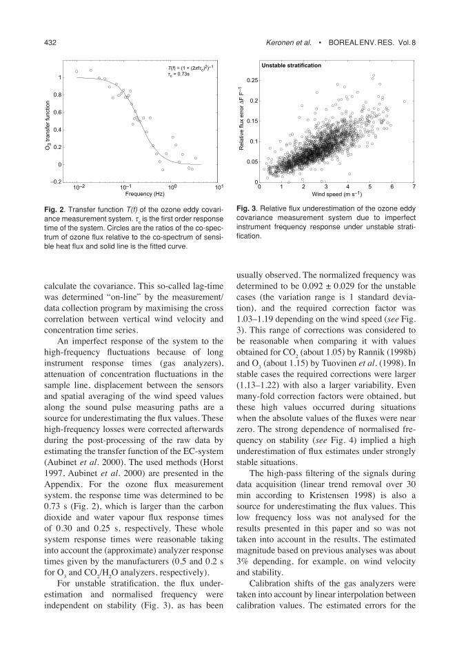
An imperfect response of the system to the high-frequency fl uctuations because of long instrument response times (gas analyzers), attenuation of concentration fl uctuations in the sample line, displacement between the sensors and spatial averaging of the wind speed values along the sound pulse measuring paths are a source for underestimating the fl ux values. These high-frequency losses were corrected afterwards during the post-processing of the raw data by estimating the transfer function of the EC-system (Aubinet et al. 2000). The used methods (Horst 1997, Aubinet et al. 2000) are presented in the Appendix. For the ozone fl ux measurement system, the response time was determined to be 0.73 s (Fig. 2), which is larger than the carbon dioxide and water vapour fl ux response times of 0.30 and 0.25 s, respectively. These whole system response times were reasonable taking into account the (approximate) analyzer response times given by the manufacturers (0.5 and 0.2 s for O

3 and CO

2/H

2O analyzers, respectively).

For unstable stratifi cation, the fl ux under-estimation and normalised frequency were independent on stability (Fig. 3), as has been

usually observed. The normalized frequency was determined to be 0.092 ± 0.029 for the unstable cases (the variation range is 1 standard devia-tion), and the required correction factor was 1.03–1.19 depending on the wind speed (see Fig. 3). This range of corrections was considered to be reasonable when comparing it with values obtained for CO

2 (about 1.05) by Rannik (1998b)

and O3 (about 1.15) by Tuovinen et al. (1998). In

stable cases the required corrections were larger (1.13–1.22) with also a larger variability. Even many-fold correction factors were obtained, but these high values occurred during situations when the absolute values of the fl uxes were near zero. The strong dependence of normalised fre-quency on stability (see Fig. 4) implied a high underestimation of fl ux estimates under strongly stable situations.

The high-pass fi ltering of the signals during data acquisition (linear trend removal over 30 min according to Kristensen 1998) is also a source for underestimating the fl ux values. This low frequency loss was not analysed for the results presented in this paper and so was not taken into account in the results. The estimated magnitude based on previous analyses was about 3% depending, for example, on wind velocity and stability.

Calibration shifts of the gas analyzers were taken into account by linear interpolation between calibration values. The estimated errors for the

10–2 10–1 100 101

0

0.2

0.4

0.6

0.8

1

Frequency (Hz)

O3 tra

nsfe

r fu

nction

T(f) = (1 + (2pftc)2)–1

tc = 0.73s

–0.2

Fig. 2. Transfer function T(f) of the ozone eddy covari-ance measurement system. tc is the fi rst order response time of the system. Circles are the ratios of the co-spec-trum of ozone fl ux relative to the co-spectrum of sensi-ble heat fl ux and solid line is the fi tted curve.

0 1 2 3 4 5 6 70

0.05

0.1

0.15

0.2

0.25

Wind speed (m s–1)

Rela

tive flu

x e

rror D

F F

–1

Unstable stratification

Fig. 3. Relative fl ux underestimation of the ozone eddy covariance measurement system due to imperfect instrument frequency response under unstable strati-fi cation.


corresponding fl ux values after the correction were 5% for O

3, 5% for H

2O and 1% for CO

2.

Air density fl uctuations, related to simultane-ous heat and water vapour transfer, are a source for apparent fl uxes of gaseous compounds (Webb et al. 1980). No correction for density fl uctuations due to heat fl ux was needed in our measurement system because temperature fl uc-tuations were expected to be dampened in the sample line (Rannik et al. 1997). The ozone fl uxes were, however, corrected for density fl uc-tuations arising from simultaneous water vapour transfer. In most cases, this correction was less than 3% of the fl ux values.

Different source and/or sink areas at differ-ent wind direction sectors and during different atmospheric stability conditions were not taken into account. The storage or release of gas below the eddy measurement level was also not taken into account.

During the winter time, freezing conditions affected the measurements by causing the build-up of ice/frost on the anemometer transducer heads. This either completely stopped the opera-tion of the anemometer or at least induced large measurement errors making the data unusable. These phenomena were the reason for (in prac-tice) a complete lack of data during November and December. During January they most prob-ably also caused bias in the wind speed data as the situations with low wind speed were also most affected by the ice/frost build-up.

Random errors

Turbulent fl uxes averaged over a limited time period have random errors because of the stochastic nature of turbulence (Lenschow et al. 1994). The random uncertainty of each 30-minute-average fl ux was obtained as presented in the Appendix. The random errors of ozone fl uxes were most frequently around 20% of the fl ux value (Fig. 5).

Analyzer noise also contributed to the random error. Its magnitude was estimated to be less than 0.1 nmol m–2 s–1 according to Lenschow and Christensen (1985) and thus the instrumental noise was low as compared with other random errors.

Ozone concentration profi les

Comparison between fl uxes obtained with the EC and profi le methods

Ozone fl uxes were also determined by the profi le technique by applying the atmospheric surface layer similarity theory for concentra-tion profi les (measured at 16.8, 33.6, 50.4 and 67.2 m heights). The concentration profi les could be measured with the measurement system and therefore the results could be used to estimate the fl uxes with the fl ux-profi le method (Fig. 6).

10–3 10–2 10–1 100 1010

0.2

0.4

0.6

0.8

Stability (z – d)L–1

Fre

quency n

m

Stable stratification

Fig. 4. Normalized frequency response corresponding to the maximum of the co-spectrum under stable strati-fi cation (Obukhov stability length L > 0).

0 20 40 60 80 1000

0.5

1

Relative random error (%)

Fre

quency o

f occure

nce

Fig. 5. Distribution of the random error of the half hour average ozone fl uxes. The scale is obtained by normal-ising the data with the mode value. The data is from the period May–July 2003.


Similar to Rannik (1998b), the fl uxes and error estimates were obtained by applying a linear regression technique to the observed and similar-ity profi les: the fl ux concentration values were obtained by using the measured profi les and by using the Obukhov stability length obtained from EC measurements. Flux was then calcu-lated as given by Kaimal and Finnigan (1994). In general, a reasonably good correspondence between EC and profi le fl uxes was observed (Fig. 7). Random errors in the fl ux estimates caused scatter in both EC and profi le fl ux data (Fig. 8). However, for profi le fl uxes the random errors were larger.

In order to compare the diurnal variation in ozone fl uxes obtained by the two methods, average diurnal curves based on the measured half-hour fl ux values were calculated (Fig. 9). The variation range, presented by vertical bars, includes differences between days as well as random errors of fl ux estimates. The average values obtained by the two techniques were quite

similar after about 08:00. During night-time and early morning the two techniques gave fl uxes with signifi cantly different patterns: the ozone fl uxes obtained from the profi le technique indi-cated larger deposition. Generally the fl ux-profi le method is thought to be quite uncertain around sunrise and sunset hours, and this could be the reason for the large discrepancy. However, we believe that this discrepancy originated from the infl uence of ozone chemistry on the vertical fl ux, which the applied profi le technique ignored. For example Vilà-Gerau de Arellano and Duynkerke (1995) reported that in the case of a reactive compound, the vertical fl ux becomes a func-tion of height because of chemical production/depletion of the compound and so a modifi ca-tion of the fl ux-profi le similarity relationship is needed. The infl uence of chemistry was probably important during early morning hours when the chemistry time scale became comparable to the time scale of turbulent transport. The chemistry could be accelerated in the morning because of the accumulation of chemical compounds par-ticipating ozone chemistry in near-surface layer during the night.

Diurnal and seasonal variation in O3 concentrations and concentration profi les

Only the data for three above canopy heights (67.2, 33.6 and 16.8 m) and one below canopy height (4.2 m) are presented (Fig. 10). The height of the EC measurements was 23 m. The measured ozone concentrations as well as con-

19 19.5 20 20.5 21 21.5 22 22.5 23

–16

–12

–8

–4

0

Time (days)

O3 f

lux (

nm

ol m

2 s

–1)

EC

Prof.

Fig. 7. Simultaneous half hour average ozone fl uxes measured by eddy covariance and profi le method, 19–22 June 2002.

0 0.15 0.3 0.45 0.6 0.75 0.9 1.05 1.2 1.35 1.5 1.65 1.8

–30

–25

–20

–15

–10

–5

0

5

10

15

Friction velocity (m s–1)

Co

nce

ntr

atio

n d

iffe

ren

ce

[p

pb

]

–30

–25

–20

–15

–10

–5

0

5

10

15

Co

nce

ntr

atio

n d

iffe

ren

ce

[p

pb

]

(O3)16.8 m – (O3)4.2 m

(O3)16.8 m – (O3)67.2 m

(O3)16.8 m – (O3)4.2 m

(O3)16.8 m – (O3)67.2 m

February 2002

0 0.15 0.3 0.45 0.6 0.75 0.9 1.05 1.2 1.35 1.5 1.65 1.8

June 2002

Fig. 6. Differences in half-hour-average ozone concen-trations between the 16.8 and 67.2-m measurement heights and between the 16.8 and 4.2-m heights as a function of turbulence (expressed as friction velocity) in February 2002 and June 2002.


centration profi les showed both diurnal and sea-sonal behaviour (see also Fig. 6).

During summertime there was a distinct and systematic decrease in ozone concentra-tions during the dark hours of the day. This was particularly obvious for the lowest measurement height (4.2 m) when the friction velocity was low. In January, that is winter time, the diurnal variability in concentrations was not as clear. However, it became discernible already in Feb-ruary.

In October there was a clear concentration profi le above the canopy during the dark hours of the day (about 17:00–07:00). The profi le started to build up early in the afternoon even before friction velocity started to decrease, and it persisted several hours after the friction veloc-ity started to increase the next morning. Between about 11:00 and 14:00 the profi le was almost undetectable except between 4.2 m and heights above the canopy. The concentrations had a clear diurnal cycle.

Throughout February the concentration profi le was hardly detectable and there was no diurnal behaviour in the concentrations. Also the friction velocity showed only a weak diurnal pattern.

In March there was again a detectable con-centration profi le during the dark hours (about 18:00–06:00). For this month, however, the behaviour was different from that in October: the profi le started to build-up and vanished almost simultaneously with the decrease and increase of the friction velocity, respectively. The concentra-tions showed again a diurnal cycle.

In June there was a very clear concentration profi le during the dark hours (about 22:00–02:00), and it was already detectable during the afternoon. The profi le started to build up several hours before the friction velocity started to decrease. In the morning the profi le persisted several hours after the friction velocity started to increase. Between about 08:00 and 12:00 the profi le was almost undetectable. The concentra-tions had a strong diurnal cycle.

The inverse dependence of concentration profi les on turbulence, evident during the winter time, was consistent with the weakness of the vegetation uptake processes during the winter dormancy. The stronger diurnal variation in ozone concentrations and concentration profi les during summer time in comparison with that in winter time was consistent with the fact that more intense solar radiation and higher air tem-perature lead to stronger photochemically initi-ated ozone formation and destruction processes and plant stomatal activity.

–20 –15 –10 –5 0–20

–15

–10

–5

0

O3 flux, EC (nmol m2 s–1)

O3 flu

x, P

rofile

(nm

ol m

2 s

–1)

Fig. 8. Comparison between half hour average ozone fl uxes measured by eddy covariance and profi le method, 19–22 June 2002. The vertical and horizontal bars represent ± 1 standard error calculated by Eq. A6 in the Appendix.

0 3 6 9 12 15 18 21 24–15

–10

–5

0

Time (hour)

O3 f

lux (

nm

ol m

–2 s

–1)

EC

Profile

Fig. 9. Diurnal variation of ozone fl uxes during June and July 2002 as measured by eddy covariance and profi le method. Variation range (standard deviation for an hour, illustrated by vertical bars) includes differences between days as well as random errors of the fl ux estimates. Data are presented as medians of hourly average values.


5

10

15

20

25

30

35

40

45

October 2001 February 2002

0.15

0.30

0.45

0.60

0.75

0.90

1.05

1.20

1.35

Fric

tion v

elo

city

(m s

–1)

Fric

tion v

elo

city

(m s

–1)

0 2 4 6 8 10 12 14 16 18 20 22

5

10

15

20

25

30

35

40

45

Time (hours)

Concentr

ation (

ppb)

Concentr

ation (

ppb)

Concentrations: 67.2 m 33.6 m 16.8 m 4.2 m

March 2002

Friction velocity

0 2 4 6 8 10 12 14 16 18 20 22 24

Time (hours)

June 2002

0.15

0.30

0.45

0.60

0.75

0.90

1.05

1.20

1.35

Fig. 10. Diurnal profi les for ozone concentration and friction velocity in October 2001, February 2002, March 2002 and June 2002. Dash, continuous, dot and dash-dot line are for 67.2 m, 33.6 m, 16.8 m and 4.2 m measurement heights, respectively. Data are presented as medians of half-hour average values.


Ozone fl uxes

The EC method gave deposition fl ux as a direct result. Because the fl ux depends on the concen-tration, the deposition velocity was also calcu-lated in order to study the diurnal and seasonal changes. The data for O

3 concentration was

taken from the profi le measurements (geomet-ric mean of concentrations at heights 16.8 and 33.6 m) because the analyzer used in those mea-surements had a better absolute accuracy.

Both the fl ux and deposition velocity were higher during the growing season, declin-ing to values close to zero in winter. The deposition velocity had values of up to about 10 mm s–1 from June until the middle of Octo-ber (Fig. 11). Between January and April the deposition velocity was less than 1 mm s–1 but was not observed to have negative values (meaning a fl ux upwards). The deposition fl ux had a similar seasonal pattern as the deposition velocity.

During the growing season (approximately April–October) both fl ux and deposition velocity

were distinctively higher during daytime while in winter the diurnal pattern was either almost or completely missing (Fig. 12).

In October (autumn) a difference between the day and night was evident. The fl ux had a maximum at midday. The deposition velocity showed a maximum a couple of hours earlier, at about 10:00. The fl ux and deposition veloc-ity were smaller during the night-time (about 17:00–07:00) than during daytime but did not reach zero values. The daytime deposition velocities were in the range 4–6 mm s–1, whereas night-time deposition velocities were about 4 mm s–1 with the lowest values reaching almost 2 mm s–1. The fl uxes ranged from –2 to –4 nmol m–2 s–1.

In February (winter) there was no detect-able differences between the night-time (about 17:00–08:00) and daytime values. Both the deposition velocity and fl ux were small, about 1 mm s–1 and –1 nmol m–2 s–1, respectively.

In March (spring) there were no distinctive daytime peaks in the fl uxes or deposition veloci-ties. For the deposition fl ux, a slight maximum

0

10

20

30

40

50

60

70

Concentr

ation (

ppb)

–25

–20

–15

–10

–5

0

5

10

15

Flu

x (

nm

ol m

–2s

–1)

Aug. Sep. Oct. Nov. Dec. Jan. Feb. Mar. Apr. May June July

2001 2002 2002

Date

Flux

–25

–20

–15

–10

–5

0

5

10

15

Depositio

n v

elo

city

(mm

s–

1)

Aug. Sep. Oct. Nov. Dec. Jan. Feb. Mar. Apr. May June July

2001 2002 2002

Date

Deposition velocity

Fig. 11. Ozone concentrations, fl uxes and calculated deposition velocities between August 2001 and July 2002. Data are given as half-hour average values.


Fig. 12. Diurnal profi les of ozone fl uxes and deposition velocities given as medians of half-hour average values in October 2001, February 2002, March 2002 and June 2002.

–9

–7

–5

–3

–1

0

1

3

5

7

Flu

x (

nm

ol m

–2 s

–1)

Flux

October 2001

Deposition velocity

February 2002

–9

–7

–5

–3

–1

0

1

3

5

7

0 2 4 6 8 10 12 14 16 18 20 22

–9

–7

–5

–3

–1

0

1

3

5

7

Time (hours)

Flu

x (

nm

ol m

–2 s

–1)

March 2002

0 2 4 6 8 10 12 14 16 18 20 22 24

Time (hours)

June 2002

–9

–7

–5

–3

–1

0

1

3

5

7

De

po

sitio

n v

elo

city

(mm

s–

1)D

ep

ositio

n v

elo

city

(mm

s–

1)


extended from about 09:00 to 15:00, whereas for the deposition velocity the maximum was not so evident. The daytime deposition velocity was about 1 mm s–1 and during the night it decreased to slightly below 0.5 mm s–1. The daytime fl ux ranged from –1 to –2 nmol m–2 s–1. During night time the fl ux decreased to values below (towards zero) –0.4 nmol m–2 s–1.

In June (summer), the diurnal cycle was strong for both fl ux and deposition velocity. In comparison with that in October, the maximum of the fl ux was broader extending a couple of hours before and after 12:00. The maximum of the deposition velocity occurred a couple of hours earlier (at about 08:00) than in October. The daytime (about 02:00–22:00) deposition velocity ranged from 2 to 6 mm s–1. During night-time the deposition velocity was about 2 mm s–1 with even the lowest values clearly above zero. The daytime fl ux ranged from –2 to –9 nmol m–2 s–1. During night-time the fl ux was about –2 nmol m–2 s–1.

The clear difference in the deposition veloc-ity and fl ux between the summer and wintertime implies that ozone deposition was controlled by plant stomatal activity at the measurement site. However, also surface deposition could be totally different between the winter and in summer. The clear difference in their diurnal behaviour between summer and autumn was consistent with the different physiological activities of the vegetation due to the longer daytime in summer than in late autumn.

Eddy covariance ozone fl ux measurements performed by Aurela et al. (1996) over a Scots pine stand in Eastern Finland in August showed similar diurnal fl ux and deposition velocity profi les to this study. The daytime deposition velocity during the two-day measurement period was 1–5 mm s–1 (30-minute averages), compared with the median values of 2–6 mm s–1 (calculated from 30-minute averages) obtained for June in this study. Night-time values were typically less than 0.5 mm s–1 (Aurela et al. 1996). Our results indicated higher night-time deposition velocity with values of about 2 mm s–1.

Pilegaard et al. (1995) and Mikkelson et al. (2000) reported diurnal behaviours of ozone fl ux, deposition velocity and concentration above Norway spruce (Picea abies) similar to

our results above Scots pine. Pilegaard et al. (1995) conducted EC measurements at a Danish forest site that consisted of 12-m high Norway spruce. The diurnal variation of the fl ux and dep-osition velocity during ten days in June showed a broad midday peak in the fl ux and a correspond-ing peak in the deposition velocity a couple of hours earlier. The deposition velocity ranged from 3.5 mm s–1 at night to 7 mm s–1 during the day with a sharp rise at dawn and a maximum in the morning. The diurnal mean O

3 fl ux and

deposition velocity measured at a Danish site in September (Mikkelsen et al. 2000) showed a maximum at approximately the same time in the morning. Duyzer et al. (1995) reported a diurnal behaviour for the canopy resistance of ozone above an 18 to 20-m high Douglas fi r stand. The diurnal variation of the resistance to uptake during two days in July showed a broad minimum between about 10:00 and 12:00 with a sharp decrease in the morning and a slower increase during afternoon and evening. The concept “canopy resistance” used by the Duyzer et al. group comes from the widely-used resist-ance model where the deposition processes are interpreted in terms of an electrical resistance analogy, in which the transport to the surface is assumed to be governed by three resistances in series: an aerodynamic resistance for transport through the atmosphere, quasi-laminar layer resistance for transport across the layer adjacent to the vegetation surface and canopy resistance for deposition at the vegetation surface (see e.g. Seinfeld and Pandis 1998, Wesely and Hicks 2000). The inverse of the sum of the resistances is then by defi nition deposition velocity. During the day in summertime the canopy resistance is the major parameter controlling ozone deposi-tion at a maritime pine forest (Lamaud et al. 2002). Assuming that the total resistance was mainly due to the canopy resistance at our meas-urement site allowed us to compare the diurnal behaviour of the deposition velocity reported in this study and the canopy resistance reported by the Duyzer et al. group. The diurnal behaviour of the canopy resistance for ozone reported by the Duyzer et al. group was similar to our results for the ozone deposition velocity. A more detailed investigation of O

3 deposition processes is pre-

sented in Suni et al. (2003).


Conclusions

The EC instrumentation and measurement setup used in this study at the SMEAR II site in Hyytiälä worked well giving results comparable to other studies using both different and similar instrumentation. The systematic errors due to imperfect frequency response of the instrumen-tation and random errors arising from the sto-chastic nature of turbulence were estimated and found to be within reasonable limits. The ozone analyzer required regular maintenance and cali-bration. Several weeks of wintertime data was lost due to ice forming conditions rendering the anemometer inoperative.

Flux results obtained using the EC method agreed well with results from a gradient method, particularly during daytime. At night and towards the morning the fl ux results were signifi cantly dif-ferent, being indicative of an infl uence of ozone chemistry on the concentration profi les and fl uxes making the fl uxes to be a function of height.

The seasonal variation of ozone concentra-tions during the time period August 2002–July 2002 (excluding November 2001, December 2001 and part of June 2002) showed a generally higher concentration in spring as compared with those in summer and winter. The ozone fl ux and deposition velocity started to increase at the end of April and had maximum values during the summertime until the end of August. Maximum deposition velocities in October were compara-ble to the maximum values during summertime.

Distinct diurnal profi les of ozone concen-trations, fl uxes, and deposition velocities were observed in summer with highest values during daytime and lowest values at night. The fl ux and deposition velocity had maxima in the morning and before noon in contrast to the ozone concen-trations that had highest values in the afternoon. Very little diurnal variation was seen in winter.

Further studies will include analysis of ozone uptake mechanisms using the measurement data more extensively for separate evaluation of aero-dynamic, quasi-laminar layer and canopy resist-ances. Stomatal resistance will be determined and compared with non-stomatal canopy resist-ance in order to study the relative importance of these two deposition pathways. Also the observed discrepancy between the results obtained by fl ux-

profi le and EC method will be examined in order to study the signifi cance of chemistry on the ozone concentration profi les and fl uxes.

Acknowledgements: We gratefully acknowledge support from the European Commission (NOFRETETE, contract no. EVK2-CT2001-00106), the Academy of Finland (project FIGARE/CORE), and the University of Helsinki Environ-mental Research Center.

References

Altimir N., Vesala T., Keronen P., Kulmala M. & Hari P. 2002. Methodology for direct fi eld measurements of ozone fl ux to foliage with shoot chambers. Atmos. Envi-ron. 36: 19–29.

Arya S.P. 2001. Introduction to micrometeorology, 2nd ed. International Geophysics Series, vol. 79, Academic Press, London, Great Britain.

Aubinet M., Grelle A., Ibrom A., Rannik Ü., Moncrieff J., Foken T., Kowalski A.S., Martin P.H., Berbigier P., Bernhofer Ch., Clement R., Elbers J., Granier A., Grün-wald T., Morgenstern K., Pilegaard K., Rebmann C., Snijders W., Valentini R. & Vesala T. 2000. Estimates of the annual net carbon and water exchange of European forests: the EUROFLUX methodology. Advances in Ecological Research 30: 113–175.

Aurela M., Laurila T. & Tuovinen J.-P. 1996. Measurements of O

3, CO

2 and H

2O fl uxes over a Scots pine stand in

Eastern Finland by the micrometeorological eddy cova-riance method. Silva Fennica 30: 97–108.

Businger J.A. 1986. Evaluation of the accuracy with which dry deposition can be measured with current micromete-orological techniques. J. Appl. Meteorol. 25: 1100–1124.

Dabberdt W.F., Lenschow D.H., Horst T.W., Zimmerman P.R., Oncley S.P. & Delany A.C. 1993. Atmosphere sur-face exchange measurements. Science 260: 1472–1481.

Duyzer J., Westrate H. & Walton S. 1995. Exchange of ozone and nitrogen oxides between the atmosphere and conif-erous forest. Water, Air, Soil Pollut. 85: 2065–2070.

Finkelstein P.L. & Sims P.M. 2001. Sampling error in eddy correlation fl ux measurements. J. Geophys. Res. 106: 3503–3509.

Foken T.H. & Wichura B. 1996. Tools for quality assessment of surface-based fl ux measurements. Agric. For. Mete-orol. 78: 83–105.

Guenther A., Baugh W., Davis K., Hampton G., Harley P., Klinger L., Vierling L., Zimmerman P., Allwine E., Dilts S., Lamb B., Westberg H., Baldocchi D., Geron C. & Pierce T. 1996. Isoprene fl uxes measured by enclosure, relaxed eddy accumulation, surface layer gradient, mixed layer gradient, and mixed layer mass balance techniques. J. Geophys. Res. 101: 18555–18567.

Guenther A. 2002. Trace gas emission measurements. In: Burden F.R., McKelvie I., Förstner U. & Guenther A. (eds.), Environmental monitoring handbook, McGraw-Hill, chapter 24, pp. 1–12.


Horst T.W. 1997. A simple formula for attenuation of eddy fl uxes measured with fi rst-order-response scalar sensors. Boundary-Layer Meteorol. 82: 219–233.

Kaimal J.C. & Finnigan J.J. 1994. Atmospheric boundary layer fl ows. Their structure and measurement. Oxford University Press, New York.

Kristensen L. 1998. Time series analysis. Dealing with imper-fect data. Risø National Laboratory, Roskilde, Denmark.

Kulmala M., Hämeri K., Aalto P.P., Mäkelä J.M., Pirjola L., Nilsson D., Buzorius G., Rannik Ü, Dal Maso M., Seidl W., Hoffman T., Janson R., Hansson H.-C., Viisanen Y., Laaksonen A. & OʼDowd C.D. 2001. Overview of the international project on biogenic aerosol formation in the boreal forest (BIOFOR). Tellus 53B: 324–343.

Lamaud E., Carrara A., Brunet Y., Lopez A. & Druilhet A. 2002. Ozone fl uxes above and within a pine forest canopy in dry and wet conditions. Atmos. Environ. 36: 77–88.

Lenschow D.H. & Christensen L. 1985. Uncorrelated noise in turbulence measurements. J. Atmos. Oceanic Tech. 2: 68–81.

Lenschow D.H., Mann J. & Kristensen L. 1994. How long is long enough when measuring fl uxes and other turbulence statistics? J. Atmos. Oceanic Tech. 18: 661–673.

McMillen R. 1988. An eddy correlation technique with extended applicability to non-simple terrain. Boundary-Layer Meteorol. 43: 231–245.

Meyers T.P., Finkelstein P., Clarke J., Ellestad T.G. & Sims P.F. 1998. A multilayer model for inferring dry deposi-tion using standard meteorological measurements. J. Geophys. Res. 103: 22645–22661.

Mikkelsen T.N., Ro-Poulsen H., Pilegaard K., Hovmand M.F., Jensen N.O., Christensen C.S. & Hummelshøj P. 2000. Ozone uptake by evergreen forest canopy: temporal variation and possible mechanisms. Environ. Pollut.109: 423–429.

Pilegaard K., Jensen N.O. & Hummelshøj P. 1995. Seasonal and diurnal variation in the deposition velocity of ozone over a spruce forest in Denmark. Water, Air, Soil Pollut. 85: 2223–2228.

Rannik Ü., Vesala T. & Keskinen R. 1997. On the dampening of temperature fl uctuations in a circular tube relevant to the eddy covariance measurement technique. J. Geo-phys. Res. 102: 12789–12794.

Rannik, Ü. 1998a. Turbulent atmosphere: Vertical fl uxes above a forest and particle growth. Report Series in Aerosol Science. N:o 35, Finnish Association for Aero-sol Research, Helsinki, Finland.

Rannik, Ü. 1998b. On the surface layer similarity at a com-plex forest site. J. Geophys. Res. 103: 8685–8697.

Rannik Ü., Altimir N., Raittila J., Suni T., Gaman A., Hus-sein T., Hölttä T., Lassila H., Latokartano M., Lauri A., Natsheh A., Petäjä T., Sorjamaa R., Ylä-Mella H., Keronen P., Berninger F., Vesala T., Hari P. & Kulmala M. 2002. Fluxes of carbon dioxide and water vapour over Scots pine forest and clearing. Agric. For. Meteorol. 111: 187–202.

Rinne H.J.I., Guenther A.B., Warneke C., de Gouw A.D. & Luxembourg S.L. 2001. Disjunct eddy covariance tech-

nique for trace gas fl ux measurements. Geophys. Res. Lett. 28: 3139–3142.

Rondon A., Johansson C. & Granat L. 1993. Dry deposition of nitrogen dioxide and ozone to coniferous forests. J. Geophys. Res. 98: 5159–5172.

Seinfeld J.H. & Pandis S.N. 1998. Atmospheric chemistry and physics. From air pollution to climate change. John Wiley & Sons, Inc., New York, 1326 pp.

Suni T., Rinne J., Reissell A., Altimir N., Keronen P., Rannik Ü., Dal Maso M., Kulmala M. & Vesala T. 2003. Long-term measurements of surface fl uxes above a Scots pine forest in Hyytiälä, Southern Finland, 1996–2001. Boreal Env. Res. 8: 287–301.

Tuovinen J.P., Aurela M. & Laurila T. 1998. Resistances to ozone deposition to a fl ark fen in the northern aapa mire zone. J. Geophys. Res. 103: 16953–16966.

Tuovinen J.-P., Simpson D., Mikkelsen T.N., Emberson L.D., Ashmore M.R., Aurela M., Cambridge H.M., Hovmand M.F., Jensen N.O., Laurila T., Pilegaard K. & Ro-Poulsen H. 2001. Comparison of measured and modeled ozone deposition to forests in Northern Europe. Water, Air, Soil Pollut., Focus 1: 263–274.

Vesala T., Haataja J., Aalto P., Altimir N., Buzorius G., Garam E., Hämeri K., Ilvesniemi H., Jokinen V., Keronen P., Lahti T., Markkanen T., Mäkelä J.M., Nikinmaa E., Palmroth S., Palva L., Pohja T., Pumpanen J., Rannik Ü, Siivola E., Ylitalo H., Hari P. & Kulmala, M. 1998. Long-term fi eld measurements of atmosphere-surface interac-tions in boreal forest combining forest ecology, microm-eteorology, aerosol physics and atmospheric chemistry. Trends in Heat, Mass and Momentum Transfer 4: 17–35.

Vilà-Gerau de Arellano J. & Duynkerke P.G. 1995. Atmos-pheric surface layer similarity theory applied to chemi-cally reactive species. J. Geophys. Res. 100: 1397–1408.

Webb E.K., Pearman G.I. & Leuning R. 1980. Correction of fl ux measurements for density effects due to heat and water vapour transfer. Quart. J. Royal Meteorol. Soc. 106: 85–100.

Wesely M.L., Lenschow D.H. & Denmead O.T. 1989. Flux measurement techniques. In: Lenschow D.H. & Hicks B.B. (eds.), Global tropospheric chemistry, chemical fl uxes in the global atmosphere. Report of the Workshop on Measure-ments of Surface Exchange and Flux Divergence of Chemi-cal Species in the Global Atmosphere, Prepared by National Center for Atmospheric Research, Boulder, Colorado, USA, for the National Science Foundation, the National Aeronautics and Space Administration and the National Oceanic and Atmospheric Administration, pp. 31–46.

Wesely M.L. & Hicks B.B. 2000. A rewiew of the current status of knowledge on dry deposition. Atmos. Environ. 34: 2261–2282.

Zeller K.F. 1993. Eddy diffusivities for sensible heat, ozone and momentum from eddy correlation and gradient measurements. Res. Pap. RM-313. Fort Collins, CO: US Department of Agriculture, Forest Service, Rocky Mountain Forest and Range Experiment Station, 44 pp.

Zeller K.F. & Nikolov N.T. 2000. Quantifying simultaneous fl uxes of ozone, carbon dioxide and water vapor above a subalpine forest ecosystem. Environ. Pollut. 107: 1–20.

Received 28 February 2003, accepted 31 August 2003


Appendix

Correction for high-frequency losses

High-frequency losses were corrected during post-processing of the raw data by estimating the transfer function of the EC-system (Aubinet et al. 2000) and by estimating the ratio of the observed and not-attenuated fl ux (Horst 1997). The co-spectral transfer function (T( f )) of an EC system for a system behaving as a fi rst order response sensor can be described by

(A1)

where f is natural frequency and tc the (fi rst order) response time of the attenuator (sensor) (Horst

1997). The effective transfer function of the EC system can be determined experimentally by (co-)spectral analysis of measurements. The transfer function can be estimated as a ratio of co-spec-tral density of scalar fl ux relative to co-spectrum of sensible heat fl ux (Aubinet et al. 2000). Such a procedure assumes that temperature measurements are not affected by attenuation (true for a sonic anemometer) and includes normalisation with integral over frequencies not affected by attenuation (Aubinet et al. 2000).

The observed fl ux (Fm) can be formally presented as the integral over multiplication of the true co-

spectrum (Co, unaffected by frequency attenuation) with the co-spectral transfer function as

(A2)

In cases of atmospheric turbulence and transfer function a good approximation for the attenuated (observed) fl ux is (Horst 1997)

(A3)

where Ft is the true (un-attenuated) fl ux and f

m is the frequency at which the co-spectrum f Co( f )

attains its maximum value. The frequency fm

is determined by average wind speed (U), observation level (z) above displacement height (d) and also by atmospheric stability via dependence on the nor-malised frequency (n

m)

(A4)

By applying the transfer function T with a time constant 0.7 s to the co-spectrum of temperature (estimated by Fast Fourier Transform technique), the fl ux underestimation was determined. In stable cases, the dependence of n

m on the stability was established as

(A5)

where L is the Obukhov stability length and d = 10.5 m. The measured fl uxes were then corrected for frequency attenuation on a 30 min basis using the expression for fl ux underestimation (Eq. A3).

Random error due to turbulence

Turbulent fl uxes averaged over a limited time period have random errors because of the stochastic nature of turbulence (Lenschow et al. 1994). The random uncertainty of each 30-minute-average fl ux


Fm was obtained as

(A6)

where

(A7)

is the standard deviation of fl ux estimates calculated for six sub-records (N = 6) of fi ve minute dura-tion F

i, i = 1,…, N. In Eq. A7 < > denote averaging over sub-records.

Ozone ﬂ ux measurements over a Scots pine forest using eddy covariance method ... ·...

Documents

Transcript of Ozone ﬂ ux measurements over a Scots pine forest using eddy covariance method ... ·...