Overview of Wireless LAN based IndoorPositioning Systems

Kai Eckert

eckertk@rumms.uni-mannheim.de

MOBILE BUSINESS SEMINAR

Department of Computer Science IVProf. Dr. Wolfgang Effelsberg

University of Mannheim, Germany

Supervisor: Thomas King

Dec. 14, 2005

1

Contents

1 Motivation and Overview 41.1 Motivation . . . . . . . . . . . . . . . . . . . . . . . . . . . . . . 41.2 Overview . . . . . . . . . . . . . . . . . . . . . . . . . . . . . . . 5

2 Basics 52.1 Positioning Systems . . . . . . . . . . . . . . . . . . . . . . . . . 52.2 Wireless LAN . . . . . . . . . . . . . . . . . . . . . . . . . . . . . 72.3 Wireless LAN Positioning . . . . . . . . . . . . . . . . . . . . . . 8

2.3.1 General Setup . . . . . . . . . . . . . . . . . . . . . . . . 82.3.2 The mathematical model . . . . . . . . . . . . . . . . . . 92.3.3 Common aspects . . . . . . . . . . . . . . . . . . . . . . . 92.3.4 Installation Costs . . . . . . . . . . . . . . . . . . . . . . . 102.3.5 Infrastructure vs. Client . . . . . . . . . . . . . . . . . . . 102.3.6 Anonymity . . . . . . . . . . . . . . . . . . . . . . . . . . 102.3.7 Scalability . . . . . . . . . . . . . . . . . . . . . . . . . . . 112.3.8 The Signal Strength . . . . . . . . . . . . . . . . . . . . . 11

3 Wireless LAN based Positioning Systems 123.1 RADAR . . . . . . . . . . . . . . . . . . . . . . . . . . . . . . . . 13

3.1.1 Empirical method . . . . . . . . . . . . . . . . . . . . . . 133.1.2 Signal propagation model . . . . . . . . . . . . . . . . . . 143.1.3 Results . . . . . . . . . . . . . . . . . . . . . . . . . . . . 153.1.4 Experimental Setup . . . . . . . . . . . . . . . . . . . . . 15

3.2 Rice . . . . . . . . . . . . . . . . . . . . . . . . . . . . . . . . . . 163.2.1 Markov localization . . . . . . . . . . . . . . . . . . . . . 163.2.2 Tracking with Markov Chains . . . . . . . . . . . . . . . . 173.2.3 Calibration . . . . . . . . . . . . . . . . . . . . . . . . . . 183.2.4 Results . . . . . . . . . . . . . . . . . . . . . . . . . . . . 183.2.5 Experimental Setup . . . . . . . . . . . . . . . . . . . . . 18

3.3 Horus . . . . . . . . . . . . . . . . . . . . . . . . . . . . . . . . . 193.3.1 Correlation Handling . . . . . . . . . . . . . . . . . . . . . 193.3.2 Continuous Space Estimator . . . . . . . . . . . . . . . . 193.3.3 Small-Scale Compensator . . . . . . . . . . . . . . . . . . 203.3.4 Incremental Triangulation Clustering . . . . . . . . . . . 203.3.5 Results . . . . . . . . . . . . . . . . . . . . . . . . . . . . 213.3.6 Experimental Setup . . . . . . . . . . . . . . . . . . . . . 21

4 Applications and Practical Issues 214.1 Implementations and Applications . . . . . . . . . . . . . . . . . 214.2 Clues to achieve better results . . . . . . . . . . . . . . . . . . . . 23

5 Conclusion 26

1 Motivation and Overview

This paper gives an overview of Indoor Positioning Systems based on WirelessLAN. Different techniques, used by three different positioning systems, are de-scribed and compared with respect to their contribution to the robustness andaccuracy of the resulting position.

1.1 Motivation

The increasing distribution of mobile devices leads to a higher demand for the socalled location based services (LBS). LBS are a subset of context aware services.The context aware services use the context of a user to provide the service.Within this category are the personalized services in e-commerce, like the ama-zon book suggestions based on the buyers interests or last buys, but also datingplatforms for people or peronalized newsletters.LBS as special context aware services provide information using the spatialcontext of the user, for example in a car navigation system, an electronic touristguide or an emergency system. In general, a lot of locations based services giveanswer to questions like “Where am I?” or “Where is the next cinema, phone cell,gas station?” and so on. Often, more than one context is used, leading to morecomplex applications pointing a person to persons with the same interests inher environment or to a cinema, which is not only open, but where also a moviestarts within 15 minutes that perfectly meets the users flavour. An overviewon LBS can be found in [Küpper, 2005] and [Schiller and Voisard, 2004], forexample.A LBS depends heavily on the underlying positioning system, that determinesthe current location of the user. There are dedicated positioning systems like theGlobal Positioning System (GPS) or the upcoming European positioning systemGalileo (planned start: 2010) [Wikipedia, 2005a]. They calculate the positionof the user with an accuracy of about twenty meters [Wikipedia, 2005b]. Themain drawback of these systems is their dependence on a line-of-sight to thesatellites, so they are typically not usable for indoor positioning.A different approach is the localization of a user via her mobile phone in theGSM/UMTS net. This localization is mainly based on the currently used basestation. This simple approach with an accuracy of about 200 meters in citiesdown to three to four kilometers in rural areas can be approved by severaltechniques to an accuracy of up to 50 meters. This is enough for most outdoorapplications (like guiding you to the next cinema near you), but in many casesnot enough for indoor applications (like guiding you to a book in a library).There are special positioning systems for indoor purposes, based on Infrared,Ultrasound or RFID. A short overview with references to further readings canbe found at [Küpper, 2005, p. 241 ff.]. All of these systems require installationsin the building and special devices weared by the users.The increasing proliferation of wireless local area networks (Wireless LAN) leadto the development of positioning systems that solely use the existing data

provided in a Wireless LAN to determine the position of a user. There is noneed for additional installations if a Wireless LAN infrastructrure already exists(thats the case in more and more company and public buildings). Moreover,a lot of mobile devices like notebooks, Personal Digital Assistants (PDAs) andsmart phones have built-in support for Wireless LANs. The accuracy of WirelessLAN based systems is in general not as high as the accuracy of dedicated indoorpositioing systems based on Infrared or Ultrasound, but it is high enough for alot of applications.One of the most important facts of Wireless LAN based positioning is that theuser is already connected to a Wireless LAN. Location based services typicallyneed a communication infrastructure to provide the user with information. In aWireless LAN environment you can use the same infrastructure for positioningand communication.

1.2 Overview

This paper gives an overview of Wireless LAN based indoor positioning sys-tems. In Section 2, we give a short introduction to location based services andpositioning systems as part of LBS. We also mention the technical basics of po-sitioning systems, as far as they are related to Wireless LAN based positioning.At last, we provide you with a rough understanding of the technical backgroundof Wireless LANs and the common techniques used by the different positioningsystems. These systems are presented in Section 3. We focus on the similaritiesand differences of the presented systems and how they performed in the tests.Finally we have a look at some applications and other systems beyond the directscope of this paper in Section 4.

2 Basics

With this section, we describe some common aspects of positioning systems andWireless LANs.

2.1 Positioning Systems

To use the spatial context of a user, the LBS needs information about thecurrent position of the user. Their are a lot of positioning systems to determinethe absolute position of a user to a certain degree, but as mentioned in Section1.1, especially for indoor purposes most of them are not suitable. On the otherside, there is no need for an absolute positioning for some applications. TheNearMe Project described in Section 4 is an example of such an approach.The focus of this paper lies on positioning systems providing an absolute positionestimation. To gain an absolute position, there are three basic approaches:

(a) Triangulation (b) Trilateration, Source: [Wikipedia, 2005c]

Figure 1: Triangulation can be used, if two locations are known together withthe angles of each line-of-sight to a reference direction (usually north). With Tri-lateration, a position is determined by three distances to three known locations.

Triangulation, Figure 1(a). Triangulation is used, if the angles to knownlocations are given. With two known locations, the absolute position in 2D canbe determined. This approach is also known as cross bearing in the nautic.The two angles are used to determine the line-of-sights to each of the knownlocations. With the position of the locations, these lines are unique in thetwo-dimensional space and intersect in the desired position.

Trilateration, Figure 1(b). If the distance to three known locations isknown, the absolute position in 2D can be determined by the section of thethree circles around these locations.Often, combinations of angulation and lateration are used. In a GSM environ-ment for example, the angle and the distance of the mobile phone according tothe base station can roughly be estimated. This is used to increase the accuracyof positioning compared to just using the associated base station as locationestimate.

Fingerprinting. With fingerprinting, the location is estimated by comparingsome observations at the current location with observations in a database. Com-pared to the former two approaches, this requires a lot more prior knowledgeabout the environment. Fingerprinting is the most natural way of a localizationfor a human being, for example in the case of a localization by room numbersthat you compare with a building plan, by reading signs in a city and matchingthem to a city map or just by looking at a front side of a house and trying to

remember, where you have seen this house last time. From the computationalpoint of view, using fingerprinting for localization is similar to face recognition.So most of pattern recognition approaches can be used for this purpose.

2.2 Wireless LAN

Generally, if we talk about Wireless LANs, we talk about the IEEE 802.11standards group [IEEE, 2005]. Today, the most widely used standards are IEEE802.11b and IEEE 802.11g. The IEEE 802.11b standard provides a maximumraw data rate of 11MBit/s. The newer IEEE 802.11g standard is backwardscompatible with IEEE 802.11b and provides a maximum raw data rate of 54MBit/s. Both standards use an adaptive rate selection, so the maximum datarate scales back to 48, 36, 24, 18, 12, 9 and 6 MBit/s in an IEEE 802.11gnetwork and to 5.5, 2 and 1 MBit/s in IEEE802.11b networks.A Wireless LAN uses the ISM band at 2.4 GHz (ISM: free for industrial (I),scientific (S) and medical (M) use). The 802.11 standard describes 14 overlap-ping channels whose center frequencies are 5 MHz apart from the next channels.Depending on national differences, a subset of these channels are actually used,for example channels 1 to 11 in the USA and 1 to 13 in Europe.Wireless LAN clients can communicate in two modes, the infrastructure modeand the ad-hoc mode. The ad-hoc mode can be used to establish a WirelessLAN without a dedicated access point.

Infrastructure mode. In infrastructure mode the clients communicate withan access point (AP) in a point-to-multipoint configuration. To determine theAP to use, a client sends a ProbeRequest packet over every channel and checks forProbeResponse packets from one or more APs. Both client and AP measure thesignal strength (s) and the signal-to-noise ratio (SNR) of every transmission.The client simply associates with the AP providing the best s and SNR.

The signal strength and signal-to-noise ratio. The measured s and SNRcan be obtained from the hardware device driver of a Wireless LAN client. s isreported in units of dBm, the signal level according to a signal power of 1 mW:

s mW ≡ 10 log10 s dBm (1)

The SNR is expressed in dB and a signal power of s mW and a noise power ofn mW gives us a SNR of

SNR = 10 log10

( s

n

)dB (2)

According to [Haeberlen et al., 2004, p. 3], the process of probing each channeland measuring the s and SNR of each AP takes about 1.6 seconds (see Section3.2.5 for the used hardware).

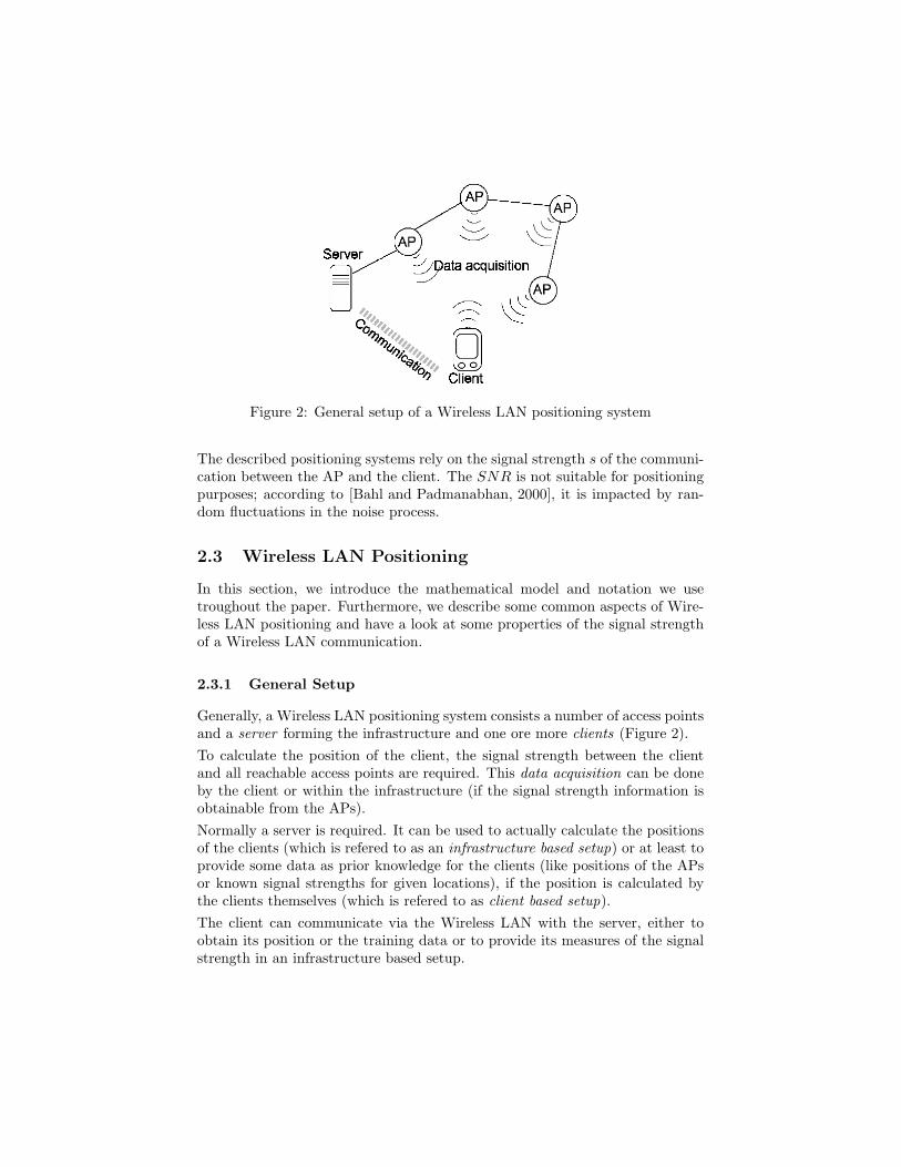
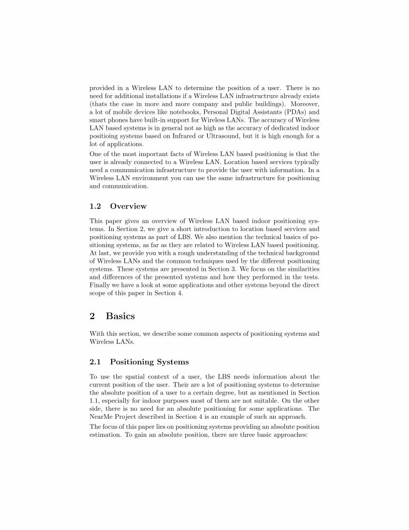
Figure 2: General setup of a Wireless LAN positioning system

The described positioning systems rely on the signal strength s of the communi-cation between the AP and the client. The SNR is not suitable for positioningpurposes; according to [Bahl and Padmanabhan, 2000], it is impacted by ran-dom fluctuations in the noise process.

2.3 Wireless LAN Positioning

In this section, we introduce the mathematical model and notation we usetroughout the paper. Furthermore, we describe some common aspects of Wire-less LAN positioning and have a look at some properties of the signal strengthof a Wireless LAN communication.

2.3.1 General Setup

Generally, a Wireless LAN positioning system consists a number of access pointsand a server forming the infrastructure and one ore more clients (Figure 2).To calculate the position of the client, the signal strength between the clientand all reachable access points are required. This data acquisition can be doneby the client or within the infrastructure (if the signal strength information isobtainable from the APs).Normally a server is required. It can be used to actually calculate the positionsof the clients (which is refered to as an infrastructure based setup) or at least toprovide some data as prior knowledge for the clients (like positions of the APsor known signal strengths for given locations), if the position is calculated bythe clients themselves (which is refered to as client based setup).The client can communicate via the Wireless LAN with the server, either toobtain its position or the training data or to provide its measures of the signalstrength in an infrastructure based setup.

2.3.2 The mathematical model

The mathematical description in the different papers was unified in this overview.Throughout this paper, we assume the following mathematical model:Generally, the localization is done by the analysis of samples of the signalstrength of the APs in communication range to an mobile device. If we have nAPs in our setup, this reads

sT = (s1, . . . , sn). (3)

All vectors s belong to the n-dimensional signal space S. On the other side, wehave the two- or three-dimensional physical space X with locations x ∈ X as

xT = (x1, x2). (4)

X can be three-dimensional with xT = (x1, x2, x3) if we want to determine alocation in three dimensions, like in a multistorey building.The localization process L itself can then be seen as

x = L(s). (5)

2.3.3 Common aspects

Proximity sensing. Proximity sensing is the simplest Wireless LAN posi-tioning system. It uses only the associated AP as information and estimates theposition of the client as the position of the AP. The accuracy is as low as therange of an AP, typically between 10 and 300 meters depending on the obstaclesbetween the AP and the client. Despite the simplicity of this approach, theirare a lot of applications that need not more accuracy than this (the GUIDEproject for example, mentioned in Section 4).

Symmetry of AP to client communication. Wireless LAN positioningsystems can calculate the position on the clients using data obtained by the clientor the position can be calculated on an external system (in the infrastructure)using data obtained by the APs. However, [Bahl and Padmanabhan, 2000, p.2] mentioned, that this decision has no impact on the accuracy of user locationand tracking; their tests showed only litte asymmetry within the precision ofmeasurements at both ends. [Ekahau, Inc., 2002, p. 2] prefers measuring onthe client side. They argue that the signals of the APs are stronger and moreconsistent as the APs are hooked up to an electricity outlet.

The multipath problem. An RF signal in an indoor environment is alwaysinfluenced by reflections, diffraction and scattering caused by obstacles withinbuildings. So in general, the signal reaches the receiver via several paths, whichis refered to as the multipath problem. The multipath problem is one reason, whya triangulation or trilateration with Wireless LAN signals is almost impossible.

Aliasing. Another problem for Wireless LAN positioning is aliasing. Alias-ing means, that there are several distinct locations receiving the same signalstrength of an AP. Even worse, due to variations in the signal strength causedby obstacles, the two locations need not to be in the same distance to the AP.This partly explains, why a trilateration of the position via the signal strengthleads not to an accurate estimate.

2.3.4 Installation Costs

The installation costs of such a positioning system are in general not as muchas for other positioning systems, assuming that there already is a Wireless LANinstallation. To get a high accuracy, the APs should overlap so that at everyposition at least two APs are reachable. But this is prefered for a stable networkcommunication, anyway. Under certain conditions, it could be reasonable toplace additional APs just to increase the positioning accuracy, see Figure 8.Every Wireless LAN compatible client should be usable for positioning. How-ever, for a client based setup, the clients need to be able to run a client softwareto calculate their positions. Most PDAs and of course every notebook shouldfulfill these requirements.In the infrastructure, a server is needed, either to provide the training datafor the clients or to perform the actual positioning. The needed performancedepends on the number of clients and if the server is dedicated for positioning,instead of being used for additional (location-based) services.

2.3.5 Infrastructure vs. Client

As mentioned in the last section, we distinguish between infrastructure basedand client based setups. The techniques proposed in this paper can be used tocalculate the position within the former or the latter. As the measured signalstrength is symmetric between the client and the AP, this decision depends onlyon application requirements. As we will see in the next sections, a client basedsetup is preferable with respect to anonymity and scalability. But if the clientsare not capable performing the calculations for positioning or if the trackingof clients without their knowledge is specially required, an infrastructure basedsetup is needed.

2.3.6 Anonymity

In an anonymous system, the client can obtain its position without knowledgeof the system. GPS, for example, is such an anonymous system. The anonymityof a Wireless LAN based positioning system depends on the general setup. Aninfrastructure based system provides no anonymity, as the position is calculatedby a central server in the infrastructure.With a client based setup, the position is calculated on the client side and isnot known by the infrastructure. However, a client cannot be anonymous if

(a) An example of the normalized signalstrength histogram from an access point.

(b) An example of the autocorrelation be-tween samples from an access point (onesample per second). The subfigure showsthe autocorrelation for the first 10 seconds.

Figure 3: Characteristics of the signal strength. [Youssef and Agrawala, 2005]

it uses the Wireless LAN, as at least the used MAC address of this client isknown in this case. In the setups mentioned in this paper, the client needs thecommunication with the infrastructure, at least to receive the training data.Furthermore, the infrastructure could calculate the position of the client on itsown and without knowledge of the client. So in general it is possible to track aclient in a Wireless LAN without its knowledge.

2.3.7 Scalability

Scalability is an issue in Wireless LAN positioning systems. Apart from thegeneral scalability of Wireless LANs, in an infrastructure based setup, the scal-ability depends on the performance of the server that calculates the position.With respect to this, a client based setup should be prefered. But the distribu-tion of the training data still restricts the scalability and needs a sophisticatedapproach like incremental updates or peer to peer distributions.

2.3.8 The Signal Strength

The signal strength is the only information we get from the APs that is usablefor the localization process. This section mentions some of the characteristicsof the signal strength:

Variations over time. As the histogram in Figure 3 shows, the signal strengthof a stationary client has significant variations over time.Further, [Youssef and Agrawala, 2005] showed, that consecutive samples of thesignal strength are strongly autocorrelated. So within a short time period, thesignal strength remains more or less constant.

Figure 4: Signal strength of three access points recorded as the user walksaround. [Bahl and Padmanabhan, 2000]

(a) Large-scale variations: Average signalstrength over distance.

(b) Small-scale variations: Signal strengthcontours from an AP in 30.4 cm by 53.3cm area.

Figure 5: Spatial variations of the signal strength. [Youssef and Agrawala, 2005]

Spatial variations. The authors of the RADAR system recorded the signalstrength of three AP while walking around a floor. As Figure 4 shows, the signalstrength of the APs rises and falls with the distance of the client.These large-scale variations are very usable for the localization process. Figure5 (a) shows a more detailed example for those. Another type of variations arethe small-scale variations. Unfortunatly, the signal-strength varies significantly,if the client is moved within centimeters (Figure 5, b). These variations arecaused by movements within the wave-length of the Wireless LAN signals (12.5cm) and by the multipath problem. Handling these variations is one of thechallenges in Wireless LAN positioning.

3 Wireless LAN based Positioning Systems

After the common introduction to Wireless LAN positioning, the following mainsection of the papers describes three positoning systems in a greater detail. In

a modular way every technique is presented and shortly described that is usedby these systems to overcome the difficulties induced by the variations of thesignal strength.

3.1 RADAR

The RADAR positioning system proposed in [Bahl and Padmanabhan, 2000]uses measurements s obtained from the APs. A set of samples is collected duringthe localization process. For the analysis, only the mean sT = (s1, . . . , sn) isused. For constant user tracking, the sample set consists of the samples obtainedin a slinding time window. For localization a nearest neighbour search in thesignal space S is used. So the signal space needs to be filled with referencelocations. Two approches are presented: an empirical method based on a set oftraining data and the usage of a signal propagation model.

3.1.1 Empirical method

The training data consists of timestamped measurements s merged with times-tamped positions recorded with the clients at 70 different locations. The authorsface the problem of variations of s with the orientation of the client by explicitlyrecording the orientation (as 1 out of 4) for each training sample. For the anal-ysis a random sample out of the training set is selected and used as input forthe nearest neighbour search in the rest of the training data, but without thesamples obtained at the same location as the input sample. Two modificationsof this method were tested among other modifications of the setup like reductionof the samples:

1. Max Signal Strength Across Orientations: The signal space is con-densed in the following way: At each location, the mean s for each ori-entation is calculated and with this four cumulated samples a resultingsample is constructed containg the maximum signal strength of each AP:sT = (max(s1), . . . ,max(sn)).

2. Multiple Nearest Neighbour: Insted of using the nearest neighbour,the location is determined by averaging the locations of k nearest neigh-bours in the signal space.

3. Continuous User Tracking: In [Bahl et al., 2000] the authors describethis modification. Based on the constraint, that the client cannot moveover a long distance in the physical space within a short time, they de-scribe an algorithm similar to the Viterbi algorithm [Wikipedia, 2005d].A history of k nearest neighbour sets in signal space is saved over a slidingwindow of h samples. Whenever a new sample is obtained, the history isupdated and the shortest path between the sets in the history is calcu-lated, linking the locations of each set with the shortest euclidean distance(Figure 6). This path can be viewed as the “most likely” trajectory of the

1 2 h...

1

.

.

.

k

Figure 6: The Viterbi-like algoritm. The vertices are the k nearest neighboursin the h sets in the history. The edges are weighted with the Euclidean distanceof the vertices in physical space. Then, the shortes path is determined (shownin bold).

client. The location of the client is associated with the start of the path.As a drawback, this modification leads to a higher latency of h signalstrength samples in the localization process.

4. Environmental Profiling: This is another enhancement described by[Bahl et al., 2000]. The signal strength varies with changes in the envi-ronment, for example with the number of people in a building. Withenvironmental profiling, the RADAR system chooses one out of a numberof training sets that has the best fit for the current environmental situa-tion. This is done by localizing the APs itself using the signal strengths ofthe other APs. As the position of the APs is known, the training set canbe determined, that currently provides the best localization. The profil-ing process runs constantly with the mean signal strengths measured in asliding time window.

3.1.2 Signal propagation model

To avoid the necessarity for the time consuming training phase, the authors alsotested their system with a signal propagation model. With this mathematicalmodel they generated a set of theoretically-computed signal strength data akinto the empirical training set.The used model is an adapted version of the Floor Attenuation Factor propaga-tion model suggested by [Seidel and Rappaport, 1992]. The authors disregardedthe effect of the floors and instead considered the effects of the walls betweenthe transmitter and the receiver. The Wall Attenuation Factor (WAF) modelis described by

s = s0 − 10r log(

d

d0

)−

{w ·W w < wmax

wmax ·W w ≥ wmax

(6)

where r indicates the rate at which the signal loss increases with distance, s0 isthe signal strength at some reference distance d0 to the AP and d is the distance

between the client and the AP. w indicates the number of walls between theclient and the AP, wmax is the maximum number of walls up to which the wallattenuation factor W makes a difference.The factors r, wmax and W have to be derived empirically. To compute thesignal strength data for a given location, the authors determined the number ofintervening walls using the Cohen-Sutherland algorithm [Foley et al., 1990].

3.1.3 Results

The median resolution of the RADAR system is in the range of 2 to 3 metersfor the empirical method and around 5 meters, if the signal propagation modelis used.The empirical method is impacted by the number of locations in the training set(significant decrease in accuracy if less than 40 locations are used), the numberof samples used for the analysis (no significant loss in accuracy, if more than twosamples are used) and the orientation of the client compared to the orientationduring the traing phase (in the worst-case, if the training set contains onlysamples of opposite orientations, the median resolution decreases to around 5meters, which is 67% worse).The use of the maximum s across orientations lead to a 9% increased resolution.The only use of the multiple nearest neighbour approach did not improve the re-sults significantly. But in combination with the maximum s across orientations,a significant enhancement of 28% could be achieved. This is due to the fact thatin this case, the k nearest neighbours in signal space necessarily correspond tok physically distinct locations.If the client is mobile and needs to be tracked instead of locating a stationaryclient, the median resolution decreases to 3.5 meters, about 19% worse thanthat for a stationary user.In [Bahl et al., 2000], the authors show, that the resolution cannot be increasedby the use of more than three APs, at least with the nearest neighbour approach.The continuous user tracking improves the median resolution significantly by29%. With this approach, a mobile client could be tracked with an medianerror distance of 2.37 meters.The environmental profiling leads to a significant enhancement of accuracy inenvironments, where the signal strengths vary strongly over time.

3.1.4 Experimental Setup

The RADAR System as described in [Bahl and Padmanabhan, 2000] is basedon the proprietary WaveLAN RF technology by Lucent. It also uses the ISMband at 2.4 GHz and is very similar to the IEEE 802.11 standards with respectto the Wireless LAN architecture and the used protocols. So the results arecomparable to the other systems.

• Access Points:

– Pentium-based PC, FreeBSD 3.0 (3 exemplars)– Digital RoamAbout NIC, based on Lucent WaveLAN RF

• Client: Pentium-based laptop, Windows 95

• Environment: Second floor of a 3-storey building, 972m2, 70 locationsin the training phase.

In [Bahl et al., 2000] the authors present some enhancements to the RADARsystem. In this paper, they use an IEEE 802.11b setup:

• Access Points: Aeronet AP4800 (5 exemplars)

• Client: Aeronet PC4800 Wireless LAN cards

• Environment: Second floor of a 4-storey building, 935m2.

3.2 Rice

[Haeberlen et al., 2004] present their positioning system that has been deployedfor testing in the Duncan Hall at Rice University (Houston, Texas). It is notnamed in a special way, so we refer to it as Rice system for convenience.

3.2.1 Markov localization

The Rice system uses a probabilistic approach. Using the Bayes Rule, the con-ditional probability P (x|s) of a location x for a given sample s can be expressedas

P (x|s) =P (s|x)P (x)

P (s)(7)

with the conditional probability P (s|x) of obtaining a sample s at location xand the a-priori probability P (x) of location x. P (s) is a normalizing constant.The Rice system uses a constant localization system, in which the unknowna-priori probability is set to the probability of the last estimate. The authorsrefer to this approach as Markov localization.

Topological model. Compared to an absolute positioning in a coordinatesystem or the positioning in a fine grained grid, like with the RADAR system,the Rice system uses a topological model of the building. The authors dividedthe whole building in cells. Most office rooms consisted of one cell, only thehallways and large rooms were devided into multiple cells, each in the size ofabout a normal office room.As a consequence, the system is not as accurate according to the actual positionof a client, but for a lot of applications, the determination of the current roomis sufficient.

Figure 7: The floor plan for part of Duncan Hall and the corresponding Markovchain. [Haeberlen et al., 2004]

Gaussian fit sensor model. For each cell in the topological model, the au-thors store only the mean µi and the standard deviation σi of the various samplesof an AP i taken in the training phase. The probability P (si = j|x) for a sig-nal strength of a single AP i and a discrete value j between 0 and 255 can becalculated as

P (si = j|x) =G(si) + β

N(8)

with the discretization G of a Gaussian probability distribution

G(si) =∫ si+1/2

si−1/2

e−(x−µi)/(2σ2i )

σi

√2π

dx (9)

and a small constant β and a normalizer N that ensures that∑255

j=0 P (si =j|x) = 1. In the performed tests the authors compare this sensor model to theconventional sensor model, where each sample s during the training phase isstored and used for the calculation of P (si|x). They refer to this model as theHistogram sensor model.

3.2.2 Tracking with Markov Chains

While the Markov localization works well for stationary clients, the use of thelast position estimation as a-priori probability harms the accuracy for a mobileclient with continuously changing position. The authors describe a solution,with which the position estimate between each set of measurements is updatedusing a Markov chain that encodes assumptions about how the client can movefrom cell to cell. The Markov chain can be thought of as a finite-state-machine(Figure 7).

3.2.3 Calibration

The Rice system uses calibration to cope with variations in the measured signalstrength due to changing environment and, very important, different hardware.The authors observed that these variations can be described by a linear trans-formation

C(s) = c1s− c2. (10)

The determination of the two parameters c1 and c2 can be done in a manual,quasi-automatic and automatic way. With manual calibration the user hasto specifiy the current cell and the system tries to estimate the parameters.Quasi-automatic calibration uses the fact, that the normalizing constant P (s)in Equation 7 remains very low for all cells, if a wrong calibration function isused. The automatic calibration proposed by the authors is not as robust asmanual or quasi-automatic calibration. It uses an expectation-maximizationalgorithm, but also a Monte-Carlo approach is mentioned that could lead to amore robust calibration.

3.2.4 Results

The tests were performed with with subsets of the training data, like with theRADAR system. The authors took at least 100 measures in each of the 510cells, thus they had a training set of about 50.000 samples.The Gaussian sensor model lead to a correct localization in over 97% of thetrials, the histogram method in over 95% of the trials. While these results seemcomparable, the Gaussian method performed better in “pathological” cases,typically returning a cell that is “off-by-one” from the correct location.To achive an accuracy of 90%, the Gaussian system needs 2 samples, with theHistogram method, 3 samples are needed. Tests with the size of the training setshow, that the Gaussian model needs only around half the size of the trainingset as the Histogram method.The AP density could be reduced to 17 APs and still the Gaussian systemcan detect the correct cell in over 90% of the trials. The Histogram methodperformed in a comparable way, but again a little weaker than the Gaussiansystem.The tracking with hidden markov-models lead to a correct localization in 71%of the trials at a speed of 4m/s. In 79% the correct cell or the previous cell waschosen (lag), and in 86% the correct cell or an adjacent cell was chosen.The calibration was tested with a time-varying environment. Due to the vari-ations, less than 70% of the localization were correct. This could significantlybe improved by calibration to 88%.

3.2.5 Experimental Setup

• Access Points: Cisco Aironet 1200 Series with 802.11a/b (27 exemplars)+ 6 other APs in adjacent buildings

• Clients:

– D-Link AirPlus DWL-650+ Wireless LAN PCMCIA cards with TIACX100 chipset

– Dell Latitude X200 laptop, Linux 2.4.25 kernel

– IBM Thinkpad T40p, Linux 2.4.20 kernel

– Driver: ACX100 (http://acx100.sourceforge.net). The driver wasmodified for stability. The code that handles the AP scanning wasoptimized to reduce the required scanning time.

• Environment: A 3-storey building with complex geometry, 135, 178m2,divided in 510 cells.

3.3 Horus

The Horus Wireless LAN Location Determination System (referd to as Horussystem) introduced by [Youssef and Agrawala, 2005] aims at two goals: highaccuracy and low computational requirements. It uses a probabilistic approachlike the Rice system with several modular enhancements to achieve an accuracyof 0.6 meters. The enhancements are suitable for other implementations, too.The authors also enhanced the RADAR system and increased the accuracy ofthe RADAR system by more than 50%.

3.3.1 Correlation Handling

Whereas the signal strength underlies variations over time, the authors showedthat the autocorrelation of successive samples collected from one AP is as highas 0.9. They propose an autoregressive model to capture this autocorrelation:

st = αst−1 + (1− α)vt; 0 ≤ α ≤ 1 (11)

where vt is a noise process and st is the stationary time series representingthe samples from one AP. Based on this model, the variance of such correlatedsamples is given by

1 + α

1− ασ2. (12)

During the training phase, the value α is estimated and stored with the dis-tribution parameters µ and σ. During the localization process, the Gaussiandistribution is adapted with the appropriate α.

3.3.2 Continuous Space Estimator

Similar to the k nearest neigbour approach, the Horus system uses a center ofmass estimation to localize the client. To do so, N locations with the highest

probability p(i) are chosen and the clients location is estimated as

x =∑N

i=1 p(i)x(i)∑Ni=1 p(i)

. (13)

The difference to the k nearest neighbour approach lies in the locations weightedby their probability p(i). This approach is accompanied by another techniquecalled time avaraging in the pysical space.With this technique, the locations of the client is estimated by avaraging thelast estimates over a sliding time window of size W like

x =1

min(W, t)

t∑i=t−min(W,t)−1

xi. (14)

3.3.3 Small-Scale Compensator

As mentioned in Section 3, the signal strength varies within small-scale changesof the clients localization. To deal with these variations, the Horus system usesperturbation of the measured sample. First, it detects a small-scale variationby calculating the distance of two consecuting location estimates. Assumingthat the client is moving constantly, the system determines to use small-scalecompensating if the distance is above a certain treshold.If such a variation is detected, the sample is perturbated. That means, artificalvariations in the samples are produced and the localization process is repeatedwith these variated samples. Then the nearest location to the last estimate istchosen as new location estimate.

3.3.4 Incremental Triangulation Clustering

This module is different from all other enhancements mentioned in this paper.Its only purpose is to reduce the computational requirements of the localizationprocess. This is achieved by clustering the environment. A cluster is defined bythe set of APs that are reachable from a location.During the localization process, the AP with the highest signal strength is chosenand only locations within clusters covered by this AP are searched. For thesecond AP, only locations covered by the first and the second AP are searchedand so on.During this process, the probabilities of the location estimate are compared. Ifthe highest estimate has a significant higher probability (by a threshold) thanthe second highest estimate, the localization stops and returns this location. Inbest case, the algorithm stops after using only one AP.

3.3.5 Results

The basic Horus system achieves an accuracy of 1.4 meters at 90% of the timeand about 2 meters in 95% of the time. This is comparable to the results ofthe Rice system, that uses also the probabilistic approach. Likewise the authorsstated a slightly advantage for a parametric method, i.e. for using a Gaussianestimator, like the Gaussian sensor model of the Rice system.The correlation handler lead to a significant increase of 19%. Moreover, theauthors showed that not using the correlation handler lead to a worse accuracyif more than two samples are avaraged for the analysis.The continuous space estimator enhanced the accuracy by more than 13% with-out time-avaraging. With time-avaraging, the performance could be increasedby more than 24%.The perturbation has a parameter to tune to achieve significant enhancements:the amount of perturbation has to be chosen. The tests showed, that the numberof APs used for perturbation is not relevant. With a suitable perturbation, theaccuracy could be enhanced by more than 25%.The clustering technique is tuned by the threshold, with which the probabil-ities of the estimated locations are compared. Depending on that threshold,the number of consulted APs in the localization process changes. Unsurpris-ingly, the accuracy increases with the number of APs. But the reduction of thecomputational effort can be more than a magnitude. According to the authors,Horus needs onl 250 multiplications compared with 2708 multiplications neededby the RADAR system.

3.3.6 Experimental Setup

• Access Points: Cisco Access Points (21 exemplars)

• Clients:

– Orinoco Silver Card, 11 MBit/s

– Testbed 1: Windows XP, Testbed 2: Linux (Kernel 2.5.7).

• Environment: Testbed 1: 4th floor of a building, 1766m2, 172 referencelocations; Testbed 2: 432m2, 110 reference locations.

4 Applications and Practical Issues

4.1 Implementations and Applications

Ekahau, Inc. Ekahau, Inc. provides a commercial Wireless LAN positioningsystem, called Ekahau Positioning Engine 2.0 [Ekahau, Inc., 2002]. The detailsof the system are not publicly available. Ekahau uses a probabilistic approach,

like Rice and Horus, based on the Bayes Rule. The actual localization is doneby fitting the samples to a probabilistic model. This localization is enhancedby rail tracking, an approach that uses a Hidden Markov Model. The resultspresented in [Ekahau, Inc., 2002] are in the range of the results of the horussystem.

The GUIDE Project. The GUIDE project has been developed to providecity vistors with a hand-held context-aware tourist guide [Cheverst et al., 2000].Whereas the system is rather an outdoor positioning system and thus beyondthe scope of this paper, the application itself is interesting. The authors identifythe following requirements for such a context-aware applicaton:

• Flexibility: If some contents (or a guided tour) are provided, the userhave to be able to decide, when, which part and with which speed he canuse the system.

• Context-Aware Information: The information should be adapted tothe context of the user, both the personal context like her role, personalinterests, tasks and her environmental context like her position, the day-of-time (think of opening times of the cafeteria being involved in thisadaption).

• Support for Dynamic Information: The system must be able to pro-vide current changes in the information, like changed opening-times, re-port of a defect printer and so on.

• Support for interactive Services: The system should provide interac-tive capabilities like messaging with other users, reserving a room for aconference, calling for a taxi and so on.

NearMe. Another interesting project is the NearMe Wireless Proximity Server[Krumm and Hinckley, 2004]. It uses a completely different approach of deter-mining objects and persons in the proximity of a client, instead of trying toestimate the absolute position.The NearMe system consists of a server and the clients. The clients are availablefor different Windows systems, but the server communicates over an open SOAPinterface, so a new client can easily be built.The clients can register themselves to the server and send a Wireless LANsignature, consisting of a global unique identifier (GUID), a timestamp anda set of MAC addresses of APs in their range and the corresponding signalstrengths. During registration, the client can specify a certain type, which canbe a person of course, but also a non-person type like a conference room, aprinter or a cafeteria.The non-person types can be used to tag an object or a location with a WirelessLAN signature.

After the registration and the submitting of the current Wireless LAN signature,the client receives two lists. One contains persons and other objects in the shortrange proximity, meaning, they are in the area of an AP that is also in the clientsrange. The other list contains persons and objects in a long range proximity,meaning, they are reachable over the areas of overlapping APs that also overlapswith an AP in the clients range.The proximitiy for the short range list is estimated by an analysis of the WirelessLAN signatures of both the client and the person or object in question. Theauthors extract the following features from this signature:

• The number of APs in common between the two signatures.

• A correlation coefficient, representing how common the signal strengthsfor the APs are.

• The sum of squared differences of signal strength.

• The number of APs in each signature that are not in common.

Using these features and a lot of training data, the authors fitted a polynomialfunction to weight these features and to calculate the proximity.For long range proximities, the estimated time is given to move from the currentposition to the target. To achieve this, the NearMe server analyses the data inits database and calculates for each pair of overlapping APs a time interval thatis needed to move from one AP to the other. With data recorded in the past,when a client sended signatures while moving from one AP to the other, theserver can take the difference of the timestamps as time-estimate.NearMe is different from the other systems in the way that it gives no absoluteposition and no guidance how to reach a destination. In return, it doesn’t needany training and works out of the box, as long as there are clients or taggedobjects close-by.

4.2 Clues to achieve better results

Ekahau, Inc. provides a guide for achieving better accuracy with her positioningengine [Ekahau, Inc., 2003]. Some of the results are mentioned here becausethey are vaild for other systems and approaches, too.

Asymmetric coverage. Especially for two APs and large areas, it is pos-sible to get a symmetric coverage, like in Figure 8. In this case, the systemcannot differentiate between the area of the upper left corner and the area ofthe lower right corner. So APs should be placed in a way that they cover thearea asymmetric.To avoid these problems, a third antenna should be used for large areas. If ahigher accuracy is needed, the use of directional antennas is recommended (Fig-ure 9), of course this often leads to additional costs especially for the positioningpurpose.

Figure 8: Symmetric coverage, two omnidirectional antennas in opposite cornersof an open space. [Ekahau, Inc., 2003]

(a) Omnidirectional antennas (b) Directional antennas

Figure 9: Different antennas.[Ekahau, Inc., 2003]

Figure 10: Significant signal variations within one area. [Ekahau, Inc., 2003]

Figure 11: Sample point on edge of adjacent area. [Ekahau, Inc., 2003]

Coverage of logical areas. To get a better localization result for practicalpurposes, the position of the reference locations should be chosen with care. Ingeneral, at least one reference location should be placed in every logical arealike a room or a part of a hallway. In a more complex area, like the corner of ahallway, the variations of the signal strength can vary strongly. In such areas,the reference locations should reflect these variations (Figure 10).The placement of reference locations near shared edges (including walls) shouldalways be avoided (Figure 11). In most cases, a worse localization in the correctroom is prefered to an almost exact absolute position estimation within half ameter, but behind a wall in the next room.

5 Conclusion

With this paper we tried to give a rough overview of existing localization ap-proaches in Wireless LANs and how they deal with the rather awkward envi-ronment of a Wireless LAN regarding the localization.The results of all approaches are very encouraging and they all showed, that itis possible to implement practical Location based services on top of a WirelessLAN positioning system.The main advantages for all proposed systems are:

• No need for additonal hardware, every existing Wireless LAN environmentcan be used.

• Additonal possibilities for applications due to the permanent connectionwith a full ethernet, if necessary with access to the internet.

• High accuracy compared with systems like GPS or GSM/UMTS

To choose a best system out of the presented systems is not necessary, as theauthors of the Horus system mentioned, every system can be improved by thepresented techniques. So the best results are achievable, if most, if not all of thepresented enhancements are implemented. A basic design decision may be tochose a probabilistic approach, like the Rice and the Horus system, they provedto be more accurate than the empiric approach.For a real-life implementation, the distribution of the training-data to the clientsand the auto-updating and recalibrating are of course steps that need attention.The further challenges in Wireless LAN positioning are the development of a self-learning process that completely removes the training phase and automaticallyadapts with the changing environment.

References

[Bahl et al., 2000] Bahl, P., Balachandran, A., and Padmanabhan, V. (2000).Enhancements to the RADAR User Location and Tracking System.

[Bahl and Padmanabhan, 2000] Bahl, P. and Padmanabhan, V. N. (2000).RADAR: An In-Building RF-Based User Location and Tracking System. InINFOCOM (2), pages 775–784.

[Cheverst et al., 2000] Cheverst, K., Davies, N., Mitchell, K., and Friday, A.(2000). Experiences of Developing and Deploying a Context-Aware TouristGuide: The GUIDE Project. In MobiCom 00, pages 20–31. ACM Press.

[Ekahau, Inc., 2002] Ekahau, Inc. (2002). Ekahau positioning engine 2.0. Tech-nical report, Ekahau, Inc.

[Ekahau, Inc., 2003] Ekahau, Inc. (2003). Guide for achieving better positioningaccuracy using positioning engine 2.0. Technical report, Ekahau, Inc.

[Foley et al., 1990] Foley, J. D., van Dam, A., Feiner, S. K., and Hughes, J. F.(1990). Computer graphics: principles and practice (2nd ed.). Addison-WesleyLongman Publishing Co., Inc., Boston, MA, USA.

[Haeberlen et al., 2004] Haeberlen, A., Flannery, E., Ladd, A. M., Rudys, A.,Wallach, D. S., and Kavraki, L. E. (2004). Practical Robust Localization overLarge-Scale 802.11 Wireless Networks. In MobiCom 04, pages 70–84. ACMPress.

[IEEE, 2005] IEEE (2005). IEEE-SA GetIEEE 802.11 LAN/MAN WirelessLANS. http://standards.ieee.org/getieee802/802.11.html. [Online;accessed 09-December-2005].

[Krumm and Hinckley, 2004] Krumm, J. and Hinckley, K. (2004). The NearMeWireless Proximity Server. In UbiComp 2004. The Sixth International Con-ference on Ubiquitious Computing, Nottingham, England, pages 283–300. Mi-crosoft Research, USA.

[Küpper, 2005] Küpper, A. (2005). Location-Based Services. John Wiley &Sons Ltd., Chichester.

[Schiller and Voisard, 2004] Schiller, J. and Voisard, A. (2004). Location-BasedServices. Morgan Kaufmann Publishers.

[Seidel and Rappaport, 1992] Seidel, S. Y. and Rappaport, T. S. (1992). 914MHz path loss prediction model for indoor wireless communications inmultifloored buildings. IEEE Transactions on Antennas and Propagation,40(2):207–217.

[Wikipedia, 2005a] Wikipedia (2005a). Galileo positioning system —Wikipedia, the free encyclopedia. http://en.wikipedia.org/w/index.php?title=Galileo_positioning_system&oldid=29937262. [Online; accessed04-December-2005].

[Wikipedia, 2005b] Wikipedia (2005b). Global Positioning System —Wikipedia, the free encyclopedia. http://en.wikipedia.org/w/index.php?title=Global_Positioning_System&oldid=29915239. [Online; accessed03-December-2005].

[Wikipedia, 2005c] Wikipedia (2005c). Trilateration — Wikipedia, thefree encyclopedia. http://en.wikipedia.org/w/index.php?title=Trilateration&oldid=28677882. [Online; accessed 12-December-2005].

[Wikipedia, 2005d] Wikipedia (2005d). Viterbi algorithm — Wikipedia, the freeencyclopedia. http://en.wikipedia.org/w/index.php?title=Viterbi_algorithm&oldid=30049724. [Online; accessed 10-December-2005].

[Youssef and Agrawala, 2005] Youssef, M. and Agrawala, A. (2005). The Ho-rus WLAN Location Determination System. In International Conference onMobile Systems, Applications And Services, pages 205–218.