Outer billiards, digital filters and kicked Hamiltonians
72
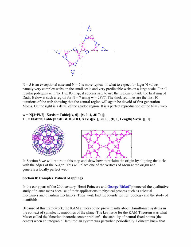
Outer Billiards, Digital Filters and Kicked Hamiltonians G.H.Hughes In 1978 J̈ rgen Moser [JM4] suggested the outer billiards map (Tangent map) as a discontinuous model of Hamiltonian dynamics. A decade earlier, J.B. Jackson [JKM] and his colleagues at Bell Labs were trying to understand the source of self-sustaining oscillations in digital filters . Some of the discrete mappings used to describe these filters show a remarkable ability to 'shadow' the Tangent map when the polygon in question is regular. Other investigators have noticed a resemblance, but there is no published theory covering the dynamics of regular polygons under the Tangent Map. In this paper and at DynamicsOfPolygons.org we outline such a theory and show how it relates to the digital filter map. In 1997 Peter Ashwin [AP] showed that the digital filter map is equivalent to a sawtooth version of the Standard Map. For regular polygons, this provides a link between the global dynamics of the Tangent map and the toral dynamics of the Sawtooth Standard Map. A.J.Scott,et al. [SHM] used a version of the kicked harmonic oscillator from quantum mechanics, to create a mapping with also 'shadows' the Tangent map for regular polygons, but in a global form. Peter Ashwin noted that the complex valued version of this map is a special case of a Goetz Map [G1]. We have modified this map to obtain a more consistent conjugacy with the Tangent Map. It is our premise that the geometry revealed by the Tangent map is intrinsic to the polygon itself and there is much evidence that points in that direction - including the contents of this paper which implies that the Tangent map is just one of many ways to illuminate this structure. Mathematica code is available for all mappings either here and at DynamicsOfPolygons. This is a survey paper which covers a number of different topics so the reader is encouraged to use the table of contents below to skip around. We have included a brief introduction to Hamiltonian dynamics in Section 4.
Transcript of Outer billiards, digital filters and kicked Hamiltonians

Outer Billiards Digital Filters and Kicked Hamiltonians GHHughes
In 1978 J rgen Moser [JM4] suggested the outer billiards map (Tangent
map) as a discontinuous model of Hamiltonian dynamics A decade earlier
JB Jackson [JKM] and his colleagues at Bell Labs were trying to
understand the source of self-sustaining oscillations in digital filters Some
of the discrete mappings used to describe these filters show a remarkable
ability to shadow the Tangent map when the polygon in question is
regular
Other investigators have noticed a resemblance but there is no published
theory covering the dynamics of regular polygons under the Tangent Map
In this paper and at DynamicsOfPolygonsorg we outline such a theory and
show how it relates to the digital filter map
In 1997 Peter Ashwin [AP] showed that the digital filter map is equivalent
to a sawtooth version of the Standard Map For regular polygons this
provides a link between the global dynamics of the Tangent map and the
toral dynamics of the Sawtooth Standard Map
AJScottet al [SHM] used a version of the kicked harmonic oscillator
from quantum mechanics to create a mapping with also shadows the
Tangent map for regular polygons but in a global form Peter Ashwin noted
that the complex valued version of this map is a special case of a Goetz
Map [G1] We have modified this map to obtain a more consistent
conjugacy with the Tangent Map
It is our premise that the geometry revealed by the Tangent map is intrinsic
to the polygon itself and there is much evidence that points in that direction
- including the contents of this paper which implies that the Tangent map is
just one of many ways to illuminate this structure Mathematica code is
available for all mappings either here and at DynamicsOfPolygons
This is a survey paper which covers a number of different topics so the
reader is encouraged to use the table of contents below to skip around We
have included a brief introduction to Hamiltonian dynamics in Section 4
Contents
1 Digital filters and the Tangent Map
11 Piecewise toral isometries
12 2kN Lemma
13 4k+1 Conjecture
2 Digital filters in 3-dimensions
3 Dynamics of an analog to digital converter
4 Hamiltonian dynamics
41 The Standard Map
42 The delta kicked rotor
43 Cold atoms-the delta kicked rotor in quantum physics
5 The Sawtooth Standard Map
6 The kicked harmonic oscillator (KHO)
61 The Web Map
62 Harpers Kicked Map and chaotic transport in lattices
7 Dissipative kicked harmonic oscillator (DKHO)
8 Complex valued mappings
81 The KAM Theorem and irrationally indifferent fixed points
82 Siegel disks and Julia sets
83 Return to DKHO
9 Bibliography
10 Summary of dynamics of the Tangent Map
11
12
Section 1 Digital Filters and the Tangent Map
Below is the schematic for a second order Digital Filter with two feedback loops Circuits such
as these are fundamental building blocks for more complex structures such as Analog to Digital
Converters JB Jackson and his associates at Bell Labs noted that such circuits can display
large oscillations even when no input is present This is due to non-linearities which can occur
when the accumulator overflows
The circuit shown here consists of three registers with a time delay of one unit between them
The intermediate outputs y(t) and y(t+1) are multiplied by b and a and fed back in where they are
added to the contents of the accumulator
The equation for the output is y(t+2) = f [ by(t) + ay(t+1) + x(t+2)] which is a second-order
difference equation Under ideal conditions the function f would be the identity function but
since the registers have finite word-length there is the issue of possible overflow
Following studies by Chua amp Lin [C1] and Anthony Davies [D] we are interested in the self-
sustaining oscillations which can occur even when there is no input so we will assume x(t) = 0
for all t The corresponding second-order equation can be reduced to two first order equations by
setting x1 = y(t) and x2 = y(t+1) Then at each time tick x1 rarrx2 (by definition) and x2 rarr f [bx1
+ ax2] If the accumulator has no overflow f is the identity function and the state equations are
1 1
2 2
( 1) ( )0 1
( 1) ( )
x k x k
x k x kb a
or X(k+1) = AX(k) where A=
0 1
b a
and X = 1
2
x
x
In this linear system the fixed point is at the origin and the local behavior is determined by the
eigenvalues which are 2( 4 ) 2a a b They are complex when 2 4b a and in this case
they have the form ie
where2 b and arccos( 2)a
When |b| lt 1 solutions will damp
out in time and when |b| gt 1 solutions will diverge When b = -1 the origin is a center and
solutions will rotation by θ This is what circuit engineers call a lossless resonator or a digital
oscillator So the b term controls damping and the a term controls the frequency In a digitally
tuned oscillator for a radio the a term would be adjusted to match the frequency of the station so
that they would be in resonance
The registers are assumed to have fixed length so the largest possible value would be
asymp 1 Negative number are typically stored in 2s complement form so the
smallest possible value is = 1 This means that the accumulator function f
has the form of a sawtooth f[z_]= Mod[z + 12] - 1
The discontinuity occurs in two possible scenarios (i) Overflow occurs when we attempt to add
one bit to asymp 1 and it becomes = 1 (ii) Underflow occurs
when we try to subtract one bit from = 1 and it becomes asymp
1 In both case the jump is of magnitude 2 The problem is that and
are only one bit apart so there is a wormhole connecting and -
The ramps shown here look smooth but actually they have discrete steps - one for each bit For
large register size f is a good approximation With the assumption that b = -1 then
arccos( 2)a and the lone parameter can be either a or θ The system equations are
1
1
( )
( ) ( )
k k k k
k k k k k k
x x f y yf A
y y f x ay f x ay
where f is defined above Note that f(yk) = yk because yk is in range by assumption
In Mathemaica Df[x_y_]=y f[-x + ay]
Df [z] Az has only three possible values 02-2 so the system equations can be rewritten to
show this explicitly
1
1
0 1 0
1 2
k k
k
k k
x xs
y ya
where 01 1ks
For initial conditions x0y0 the corresponding sk sequence can be obtained by generating the
orbit with Df and then applying the following function to each point in the orbit
1 1
[ ] 0 1 1
1 1
if x ay
S x y if x ay
if x ay
In Mathematica S[x_y_]=Which[-x + a]y gt= 1 1 -x +ay lt -1 -1 True 0]
For example Orbit = NestList[Df x0y0100] S-sequence = SOrbit
The space in which Df operates is [-11)2 so it is a map on a 2-Torus T
2 rarr T
2 Since Det[A] = 1
this map preserves area so it is a symplectic map Symplectic maps on tori have been an area of
interest to mathematicians and physicists since Henri Poincare (1854-1912) realized their value
in the analysis of conservative (Hamiltonian) systems
Any linear map of the form A= 0 1
1 a
will always be symplectic This implies that the
eigenvalues have the form λ and 1 λ and as we noted above 2( 4) 2a a so for
(02)a the eigenvalues are complex with unit absolute value so λ =2 ie
where θ = arccos(a2)
This implies that A represents a rotation but it is an elliptical rotation which can be conjugated
to a pure rotation When studying the dynamics of maps based on matrices such as A if the trace
a is the solution to a polynomial equation of low degree there are computational advantages
(exact arithmetic) to leaving A in its original form and we will work with A in both its original
form and the conjugate form
The Jordan normal form of A is a rotation matrix R 0 1
1 2cos
~ cos sin
sin cos
Note that R is actually a rotation by θ which is perfect for the canonical clockwise rotations of
the Tangent MapThe conjugating matrix is
G = 1 0
cos sin
with G-1
= 1 0
cot 1 sin
Maps of this form have been studied by many authors As dynamical systems they are known as
piecewise affine maps on the torus or piecewise toral isometries Arek Goetz [G2] defines the
general form to be 0 1
1 2cos
x xF
y y
where F is defined Mod 1 so F[01]
2rarr[01]
2
Note that the matrix here is the transpose of A so F is a Mod1( toral) version of the linear Df
map Even though the defining matrices for Df and F are linear the Mod 1 condition means the
global dynamics are far from linear For F the rational rotations θ will yield dynamics which are
similar to the Tangent Map but there are significant differences These differences disappear with
Df when f is turned on The following affine version of F has also been studied and it should not
be too surprising that it is conjugate to Df (with f turned on) when β = 0
0 1 1( 0)
1 2cos cos
x x orF
y y
Example F[x_ y_] = Mod[-y + 1 x + 2Cos[w]y - Cos[w] 1] w = 2Pi14
H0 = Table[x 0 x 0 1 001] (use this to scan the x-axis to depth 200)
Web = Flatten[ Table [NestList[F H0[[k]] 200] k 1 Length[H0]] 1]
TG[x_ y_] = x + yCos[w] ySin[w] (Transpose of G above)
Graphics[PointSize[10] Magenta Point[Web] Blue Point[TGWeb] Axes-gtTrue]
We will see that these images are transposed and scaled copies of the Df webs Both give perfect
Tangent map webs for the regular 14-gon
Sections 5 6 and 8 will discuss the connection between these maps and Hamiltonian dynamics
If a matrix such as A was the Jacobian of a Hamiltonian system the combination of complex
eigenvalues and Det[A] = 1 would imply that the origin is a marginally stable fixed point where
the stability depends on θ When the system is perturbed the rational and irrational rotations
would yield different dynamics and the KAM Theorem gives conditions for the survival of a
non-zero measure of the irrational rotations
The full Df map includes a perturbation but the perturbing function f is discontinuous and this is
at odds with the KAM Theorem where any perturbation is assumed to be at least continuous In
fact Jurgen Moser proposed the Tangent Map as an example of a system that violated the
continuity conditions of the KAM Theorem - but retained some of the same characteristics It
appears that the Df map is a perfect Mod 1 model of the Tangent Map when the polygon is
question is regular
The Df map and related maps with sawtooth nonlinearities are similar tokicked Hamiltonians
where the perturbing kicks are periodic If the kicks are relatively small they can be used to
model continuous perturbations such as planetary interaction The Standard Map is a kicked
Hamiltonian where the kicks strength can adjusted to see what happens when the KAM Theorem
breaks down
In the Standard Map the coordinates represent angular position (x) and angular momentum (y)
and the perturbing function is naturally of the form Ksin( )x For Df the perturbation frequency
depends on the parameter a so it remains fixed This means that the Df map can be tuned and
the Standard Map cannot For the Tangent Map this is critical since the perturbation frequency is
fixed by the regular polygon There is a version of the Standard map which retains this ability to
be tuned Peter Ashwin calls it the Sawtooth Standard Map and in Section 5 he shows that it is
conjugate to Df
Definition of the Tangent Map Given a convex N-gon with a clockwise (or counter-clockwise)
orientation pick a point p outside the N-gon and draw the tangent vector (supporting line) in the
same orientation as the n-gon Extend this line segment an equal distance on the other side of the
point of contact The endpoint of this line segment is called τ(p) so τ(p) is the reflection of p
about the point of contact Therefore τ(p) = minus p + 2c where c is the point of contact So τ is a
piecewise linear map (piecewise isometry) where each lsquopiecersquo corresponds to a different vertex
of the N-gon
For most N-gons and most initial points the orbits under τ are periodic Below is an example of
a periodic orbit for the regular heptagon N = 7 The large buds map to each other with period 7
The connection between the Tangent Map and Df is surprisingly close - when the polygon under
study is regular For example the regular 14-gon has generating angle θ = 2Pi14 and if we set
a= 2Cos[2Pi14] and define the linear map as A=01-1a X[x_y_]=Axy The
orbit of 11 will be a perfect elliptic 14-gon (For reference we have also drawn the
boundaries of the Df region H0=111-1-1-1-1111)
Graphics[RedLine[NestList[X1114]] Black Line[H0] Axes-gtTrue]
To transform Df space to Euclidean metric space use G and its inverse from above In
Mathematica it is more efficient to write the matrices as transformations
G[x_y_]=x xCos[w]+y Sin[w] GI[x_y_]=x-xCot[w]+(ySin[w])
Graphics[RedLine[GINestList[X1114]]BlackLine[GIH0]Axes-gtTrue]
Now the elliptic 14-gon is a perfect regular 14-gon To make this rhombus match canonical
Tangent space we will rotate by π2 (Note that this step was not necessary with F which was
Tranpose[A])
DfToTs[A_] = RotationTransform[Pi2][GIA]
TsToDf[A_] = GRotationTransform[-Pi2][A]
Graphics[RedLine[DfToTs[NestList[X1114]]]BlackLine[DfToTs[H0]]Axes-gtTrue]
(We will call this rhombus space (or sometimes Trapezoid space) It is embedded in Euclidean
Tangent Map space which is why we also use the name Ts space Occasionally we will need to
make the distinction between this space and global Tangent Map space)
To get a feeling for the dynamics of Df we can scan the top edge which is the overflow line
Below are the first 4 iterations of this scan followed by a depth 200 scan
H0 = Table[x1 x-11005]
Graphics[Point[Flatten[Table[NestList[DfH0[[k]]200]k1Length[H0]]1]]]
Mapping this back to Tangent space gives a perfect Tangent Map web for the regular 14-gon
The green dots are the centers of the second generation heptagon Mom[1] in Df space and
Tangent space We will compare their orbits below It is possible to track the dynamics of the
regular heptagon N = 7 within the context of N = 14 but it would be preferable to use the
heptagon as the generator To see why we cannot do this suppose we set a = 2Cos[2Pi7] and
repeated the web from above The linear map will generate a perfect elliptic heptagon as shown
on the left below but when Df is turned on this heptagon will be chopped up by the boundary
conditions and become a 14-gon Below are the first 4 iterations of the Df web and then the
level-200 web
This scenario is not limited to the Df map It is an issue with most piecewise toral isometries
There is no natural way to make the odd rotations conforming so there is no way to avoid this
carnage The limiting Df webs for θ = 2Pi14 and θ = 2Pi7 are quite different even though the
resulting ellipses are both regular 14-gons The differences in the dynamics show up very early
in the developent of the webs The θ = 2Pi7 web forms its edges in a mod-2 fashion This
leaves an imprint on the subsequent dynamics The major effect is a truncation of the web as we
can see below These differences persist even for large N
The S[2] buds for N= 7 are canonical 14-gons which have a step-2 orbit The limiting structure
shown above for θ = 2Pi7 is an exact match for the local S[2] dynamics of N = 7 Below is
DfToTs[DfWeb] We will discuss its dynamics in detail later in this section
The case for N = 7 does not generalize and except for N = 5 the remaining θ = 2PiN cases
for N prime have dynamics which we cannot identify For example the Df dynamics of w =
2Pi11 and w = 2Pi13 are quite unique an only marginally related to the actual dynamics of N
= 11 and N = 13 Yet the Df dynamics of w = 2Pi22 and w = 2Pi26 give perfect copies of the
webs of N = 11 and N = 13
Symbolic Dynamics
For or any given value of θ Df space is partitioned into 3 regions by S These regions are shown
below for θ = 2Pi14 overflow at top (represented by lsquo1rsquo) in bounds (lsquo0rsquo) and underflow (lsquo-1rsquo)
For a given initial point the s-sequence tracks the movement of the point relative to these
regions The dividing lines are the only discontinuities of f in the interior of this region so the
behavior of the system within each region is linear and well understood To analyze the
dynamics of an orbit the real issue is how the points move between regions
The study of these sequences is called symbolic dynamics and was pioneered by George
Birkhoff [GB] (1884 1944) Many studies have been done to analyze the admissable sequences
of the Df map and to determine how they relate to the dynamics For example Chua amp Lin [C1]
have shown for the Df map with a non-zero (i) no sequence can have 11 or -1-1and (ii) no
sequence can have 101 or -10-1 The Tangent Map sequences have similar restrictions
Below are the 7 regions for the regular heptagon with rotation angle w = 2Pi7 The map τ is not
defined on the trailing edges so these are the discontinuities
The s-sequence for the Tangent Map is called a corner sequence For an N-gon this sequence has
N symbols 12N Using these kicks we can rewrite the Tangent Map as
1
1
1 0 2
0 1 2
k k
k
k k
x xCs
y y
where Cj is the jth vertex of the N-gon
10 05 05 10
10
05
05
10
So on each iteration of τ the current point X is inverted and gets a position-dependent kick
2 jX X C where Cj is the jth vertex (Note that this makes the return map τ2 very
interesting since ( 2 ) 2 2( )j k k jX X C C X C C so the orbit of X is determined by a
sequence of displacement vectors and every displacement vector is a difference of two vertices)
Given an initial point the Tangent map orbit can be constructed from the corner sequence
skTaking first differences yields a step-sequence which shows how many vertices are advanced
on each iteration These step-sequences are a valuable aid in analyzing the dynamics For
example with regular polygons we can classify invariant regions based on the step
sequencesWe will do this below for the regular heptagon Step sequences lead to a natural
definition of winding number which measures the average rotation on a scale of 0 to 1
There are only a few regular polygons where we have a complete understanding of the dynamics
and the step sequences N = 34568 and 10 It is safe to say that at this time no one understands
the symbolic dynamics of any regular polygon outside this short list Cracking the code for N = 7
would be a great step forward but the dynamics here are very complex indeed
At the other extreme any polygon with rational vertices ( a lattice polygon) will have only
bounded periodic orbits By changing just one vertex of a rational Penrose Kite to irrational
Richard Schwartz [S1] has shown that unbounded orbits exist This answered a 30 year-old
question by Jurgen Moser
In his Wikipedia article on the Outer Billiards Map Schwartz lists the following as the most
important open questions
(i) Show that outer billiards relative to almost every convex polygon has unbounded orbits
(ii) Show that outer billiards relative to a regular polygon has almost every orbit periodic The
cases of the equilateral triangle and the square are trivial and S Tabachnokov answered this
for the regular pentagon
(iii) More broadly characterize the structure of the set of periodic orbits relative to the typical
convex polygon
The Tangent Map is not defined on the extended trailing edges of the polygon so τ2 = ττ is not
defined in the inverse image of these edges Continuing in this way the web of points which
must be excluded at iteration k is
0
0
W (W )j k
j
k
j
Where W0 is the level 0 web Taking the limit as krarrinfin yields the (inverse) web W (The forward
web is defined in a similar fashion using forward edges and τ and the full web is the union of
these two) The Tangent Map software will generate the forward webs to any desired accuracy
and a reflection transform will yield the inverse webs when necessary For regular polygons
these two webs can be used interchangeably The complement of the web are points where τ is
always defined We call this the genetic structure of the polygon Any affinely equivalent
polygon would have an affinely equivalent webThe same web generation process works for the
Df map because of the symmetry between overflow and underflow
The Dynamics of N = 7 (and N = 14) using Df
Based on our remarks earlier we will use θ = 2Pi14 to study the regular heptagon with Df This
means that we will be inferring the dynamics of N = 7 based on the dynamics of N = 14 This is
not a major impediment because they have conjugate webs On the left below is a vector diagram
showing the local web structure around N = 7 In the usual scenario the heptagon would be at
the origin and the 14-gon would represent a step-3 resonance of the Tangent Map In our genetic
language they form a lsquoMom-Dadrsquo pair so Dadrsquos formal name in this scenario is S[3] (There are
fundamental differences in dynamics between n-gons and 2n-gons for n odd so the gender
distinction is useful)
This diagram would be unchanged if Dad was at the origin and Mom was a step-5 resonance
Her formal name would be DS[5] which is short for lsquoDad step-5rsquo On the right below are the
step regions for Mom and Dad There is actually a DS6 which is off the screen on the right and it
is occupied by an identical Dad
The lsquobudsrsquo surrounding Dad above can be regarded as orbiting Dad or Mom This establishes a
lsquoconjugacyrsquo between the dynamics of N = 7 and the dynamics of N = 14
(In orbital dynamics satellites may have their own satellites and for point masses there is no
theoretical limit on the levels of recursion No lsquomoons of moonsrsquo are known in the solar system
but the first confirmed instance of a satellite of an asteroid came from a Galileo flyby of the
asteroid Ida in 1993 It is not uncommon for near -Earth asteroids to have such satellites but the
gravity of the Moon is too lsquolumpyrsquo to support lsquonaturalrsquo satellites)
For example below is the orbit of the intermediate-size 7-gon known as DS[3] Her period is 14
relative to Mom and her step sequence is (32) Note that she visits Dad on every third iteration so
she is 3-step relative to Dad Her orbit lsquounfoldsrsquo from a (32) to a simple 3-step as we pass from
Momrsquos world to Dadrsquos In this conjugacy the 7 Dads act as one
The Df map performs this same synthesis so it provides a natural mapping of the 7 Dads to one
This establishes a correspondence between periods of orbits as explained by the 2kN Lemma
below
Below are the first and second generations of the Tangent Map for the regular heptagon N = 7
We use the right-side Dad below because he forms the natural first generation Dad[0] in the
infinite chain of Dads converging to the GenStar point at far left As we remarked above Dad
and Mom preside over the same structure - even when Dad is the central polygon (N = 14) This
holds for any regular prime N-gon
The rectangle at the tip of Generation 1 is enlarged above to show that Generation 2 is quite
different from Generation 1 The generations form an endless chain converging to the tip which
is called GenStar -the generation star point (A regular prime N-gon has Floor[N2] star points -
including the vertex of Mom) The even and odd generations appear to be self-similar but N = 7
is the only known case where this dichotomy exists The even generations are dominated by non-
generic regular N-gons (Portal Moms) which have displaced the nornal 2N-gon S2 buds They
are called Portal Moms because of they are surrounded by intricate websThese plots are only a
portion of the full Tangent Map plot which is shown below
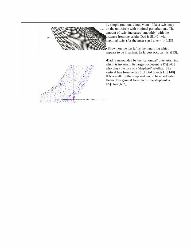
Below is a plot showing the structure of the Tangent space for N = 14 inside the first ring of
bounding Dads To make his plot compatible with the Df plot we used a central Dad with
height 1 rather than radius 1 which is the canonical size The (forward) web for N = 14 is shown
in black It is formed by scanning each of the 14 extended forward edges of Dad at increments
of 02 to a distance of 4 units taking 200 iterations of each point so the Mathematica command is
WebPoints[02 4 200]
The Magenta plot is a depth 200 scan of Df space using the overflow line at the top edgeThe
blue is a map of these points to trapezois space and the plot on the right is an overlay of 7 of
these trapezoids
The Mathematica commands for these plots are
H0 =Table[x1 x-11001] DfWeb = Flatten[Table[NestList[Df H0[[k]]200]
k1Length[H0]]1] TrWeb = DfToTr[DfWeb]
Show[Graphics[AbsolutePointSize[10]Point[TangentWeb] Magenta Point[DfWeb] Blue
Point[TrWeb]Axes-gtTrue]]
On the right-hand plot it should be clear that the overlap of the 7 trapezoids is identical to the
region not covered so the area of the central star region is exactly 7 times the area of a trapezoid
By symmetry each trapezoid accounts for exactly 17th of the tilesThis fact will allow us to
make connections between periods in Df space and periods in Tangent Space See the 2kN
Lemma below
The TrWeb can be generated about 30 times faster than the traditional Tangent Map web because
it is only necessary to scan one short edge using a much simpler algorithm - the Df map The
remarkable fact is that these two scans reveal the same structure
Example To find the orbit and S-sequence for the center of Mom[1] in Df space
In Tangent Map space cMom1 asymp -4153042-947905 The corresponding Mom[1] in Df space
has center TrToDf[cMom1] asymp -947905 947905 (These DF coordinates match because this
center lies on a line of symmetry in both Tangent map space and Df space)
Orbit = NestList[Df TrToDf[cMom1]20] Ssequence = SOrbit =10000-1100
Mom[1]s Df orbit and the s-sequence are both period 6 In the plot below we have included the
green division lines so the reader can track the orbit and compare it with the s-sequence Mom[1]
starts her life in an overflow condition (s = 1) and progresses from there to the edge of the N =
14 lsquoDadrsquo where she is lsquoin boundsrsquo (s = 0) Then next four surrogate Mom1s are also lsquoin boundsrsquo
but eventually they generate an underflow (-1) and the cycle repeats
For regular polygons every orbit in Df space has a complementary orbit which is obtained by
reflecting each point So the complementary Mom1 orbit has initial point at 947905 -947905
and symmetric dynamics The s-sequence is the complement of the original so it is
-100001 These two orbits together account for 12 Mom[1]s in Df space This implies
that the there will be 712 matching Mom[1]rsquos in Tangent space These 84 Mom[1]rsquos are
partitioned into groups of 70 and 14 as we shown below
On the left below is the Tangent space orbit of Mom[1] It is period 70 as shown by the green
dots on the left below Note that just two of these orbit points lie in the magenta Df trapezoid
Back in Df space these two are the initial points for the two Df orbits described above It would
seem that the orbit of Mom[1] in Tangent space cannot replicate the Df orbits because the outer
star region is invariant and points in the outer region never map to the inner region near Dad But
we noted earlier that Mom[1] can be regarded as lsquoorbitingrsquo Dad where the 14 Dads act as one
The step sequence for Mom1 is 66665 so the first 4 iterations skip 6 corners of Dad and the
5th iteration skips only 5 corners This sequence is repeated for each of the 14 Dads in the ring
On the right above is the first 5 iterations in this orbit This accounts for 70 Mom[1]s and the
remaining 14 are the canonical Mom[1]s on the edges of the central Dad This count must match
the Df count and this is the content of the 2kN Lemma below
The 2kN Lemma For the Df map with θ = 2Pi2N every periodic orbit in Df with (prime)
period k accounts for 2k congruent tiles in Trapezoid space and 2kN congruent tiles in Tangent
Space In Tangent space the centers of these tiles may have different periods but the sum of the
periods must be 2kN
Example ( N = 7 so the Df polygon is the 14-gon)
Tile Tangent Space center Df period (k) Periods in Tangent Space
Mom[1] -415302-947905 6 70 + 14 = 2middot6middot7
Dad[1] -389971-890084 5 56 + 14 = 2middot 5middot7
Mom[2] -435619-994274 22 126 + 126 + 28 + 28 = 2middot22middot7
To explain the last entry in the table on the left below is the period 22 orbit of Mom[2] in Df
space She is in the far left corner and her orbit includes 3 points on the edges of the local
Dad[1] On the right below the arrows point to the corresponding four points in Tangent space
Under the Tangent map τ the two magenta points map to each other with period 126 and the two
black points also map to each other with period 126
In the vicinity of Dad these Mom[2]rsquos have period 28 but the lsquoevenrsquo and lsquooddrsquo Dad[1]rsquos map to
each other so there are two groups of 28 each
Unlike Tangent space periodic orbits in Do space always have s-sequences with the same
period so Mom[2] above has a period 22 step sequence 1 0 0 0 0 -1 1 0 0 0 -1 1 0 0 0
-1 1 0 0 0 0 -1 This sequence traces out a convoluted orbit in the diagram above
These 308 points do not account for all the regions congruent to Mom[2] The 14 yellow points
on the right above are part of another Do orbit This orbit is period 86 so the 2kN Lemma says
that they represent 1204 regions in Tangent space for N = 14 The breakdown here is two outer
regions of period 476 each and two inner regions of period 126 Together these two Do orbits
account for 1512 congruent Mom[2]rsquos and this factors as 108middot14
The 2kN Lemma is just a small step toward solving the lsquoperiodicityrsquo problem for prime N-goons
There are simple formulas for the periods of the First Families but these formulas do not extend
to subsequent generations because the evolution of these generations is not well understood
except in the case of the regular pentagon Even when there appear to be well-defined sequences
of lsquoMomsrsquo and Dadrsquos converging to the local Gemstar point there are no known formulas for
their periods ndash but it does appear that the ratios of the periods approaches N + 1 This is outlined
in the 4k+1 conjecture below
4k+1 Conjecture Suppose M is a regular N-gon with N odd centered at the origin with a vertex
at 01 Define
(i) GenScale[N] = (1-Cos[PiN])Cos[PiN] (this is how generations scale under τ )
(ii) GenStar[N] =-Cot[PiN](1+Cos[PiN]) -Cos[PiN] (the point of convergence )
Suppose N is prime of the form N = 4k+1 for k a positive integer Then there will be infinite
sequences of regular N-gons M[j] (the Moms) and regular 2N-gons D[j] (the Dads) converging
to GenStar M[j] will have radius r[M[j]] = GenScale j and D[j] will have height h[D[j]] = (1 +
GenScale)middotGenScale j for j a non negative integer The center of M[k] is (1 r[M[j])middotGenStar
and center of D[j] = (1+ h[Dad[j]])middotGenStar The periods of these centers have ratios which
approach N+1
Example Below are the first three generations of Mrsquos and Drsquos for the regular pentagonIn this
case the entire family structure is preserved on each new generation but this is not typical (D[0]
cannot be seen below because he is off the picture on the right We call him DadRight)
In the case of N = 5 it is easy to see why the ratio of periods approaches 6 but the N + 1 rule is
not as obvious for N = 13 and beyond Below are tables showing the Moms periods for N = 7
and N = 13
8 Generations of Moms for N = 7
Generation Period Ratio
Mom[1] 28
Mom[2] 98 35
Mom[3] 2212 2257
Mom[4] 17486 7905
Mom[5] 433468 24789
Mom[6] 3482794 80347
Mom[7] 86639924 24876
Mom[8] 696527902 80393
6 Generations of Moms for N = 13
Generation Period Ratio
Mom[1] 130
Mom[2] 2366 18200
Mom[3] 32578 13769
Mom[4] 456638 14017
Mom[5] 6392386 13998
Mom[6] 89493950 14000
Even though N = 7 is a 4k+ 3 prime it retains some of the recursive generation structure of 4k+
1 primes but this structure appears to alternate between even and odd generations with rations 8
and 25 Numerical evidence suggests that these same ratios apply to N = 14 and to the Df map
Example N =13 has 6 star points as shown below (By convention Moms vertex is Star[1] The
corresponding Scale[1] is 1) The graphic below also shows Dads 11 star points Regular 2N-
gons have N-2 star points Each star point defines a scale and each family member is scaled
relative to their star point For example Mom[1]s radius is Scale[6] =GenScale[13] asymp0299278
If Dad were at the origin his Scale[11] would be GenScale[26] asymp 00147432980 and his
Scale[10] would be GenScale[13] The First Family shown here can be generated using just
Moms scales because her scales can be applied to Dads family members and their centers all lie
on the line of symmetry extending from the origin to GenStar
The largest bud above is called S[5] because it is step-5 relative to Mom This implies that it is
step-10 relative to Dad as we can see above The Tangent Map program will automatically
generate and display First Families for regular polygons - without the support lines
Table[scale[k] k16] will show Moms scales But for composite values of N there may be
mutations among the canonical family members
For N = 5 the sequences of Dads and Moms play a dominant role and in fact the N+1 rule
determines the fractal dimension but as N increases these sequences play a less important role
in the global dynamics The dynamics for N = 13 are very complex and these sequences are
islands of stability So there is a well-behaved generation scaling but not well-behaved
dynamics within these generations There do not appear to any self-similar copies of the first
generation but there are signs of a mod 2 dichotomy starting with generation 3
The Regular Pentagon N = 5
We cannot prove that any specific orbit for N = 7 is non-periodic but it is easy to see that non-
periodic orbits exist for N = 5 (and by implication N = 10) The regular pentagon is shown
below in standard position with vertex c1 = 01 The coordinates of a non-periodic point are s
= c5[[1]] c4[[2]] - where c5 [[1]] is the first coordinate of c5 This orbit is lsquodensersquo in the inner
web as shown in below (s asymp -095105651629515 -0809016994374947424
Passing from N = 5 to N = 10 the natural embedding uses the right-side Dad In this case the
point s is mapped to s1 = kTo2k[s] = TranslationTransform[cMom][srMom] where cMom
and rMom are the parameters of the N = 5 Mom in the context of N = 10 so rMom asymp
0552786404 and cMom asymp -170130161-055278640 This gives s1 asymp -2227032728-10
This point s1 is still non-periodic but it generates just the outer invariant annulus for N = 10
This is the blue ring shown below The inner annulus decomposes into two congruent regions ndash
each of which has their own non-periodic generator Mapping s1 to Df space yields ds1=
TrToDf[s1] = -15 (exact) Of course the orbit of ds1 is non-periodic in Df space Its image
back in Tr space is shown in magenta on the right below This is the same scenario observed
earlier with N = 7 the Df map is more faithful to the dynamics of the N-gon than the 2N-gon
This shows that the Df map is not affected by the decomposition of orbits that occur in N = 10
Clearly the ds1 orbit (magenta) together with the orbit of its reflection 1 -5 (blue) are lsquodensersquo
in the N = 5 web as we can see below By symmetry either one of these points would suffice as a
lsquogeneratorrsquo for the N = 5 web
The rationality of these limit points may be due to the fact that in Tangent space the initial non-
periodic point s1 has coordinates relative to Mom (and Dad) and under the conjugacy
transformation two of these coordinates of Dad map to 11 and -1-1 in Df space
The S-sequence of ds1 = -15 is 10-110-1hellip (This sequence must be non-periodic but it
appears that the frequency of 0 rarr 25 This is in keeping with our results for the regular
pentagon which show the orbit of s has winding number which approaches 25 It is not hard to
show that no periodic orbit can have this winding number) Of course 1-5 has the
complementary step sequence -101-101hellip with the same frequency of lsquo0rsquo
We can apply the 2kN Lemma to help understand the connection between the Df orbits and the
Tangent Map orbits For example in Df space Dad1 has period 3 so there should be 30 such
Dad1s below and the breakdown is 10 + 20 = 10 + 102 The Dad2s are period 17 in Df space
and there are 50 + 1210 Dad2s in the invariant inner star region In the special case of N = 5
there is a simple relationship between the Df periods and the N = 5 periods For k gt1 period
Dad[k] = 2Df period + 1 (The 1 is the map from one Df cycle to the other) This relationship
carries over in the limit and becomes the decomposition of non-periodic orbits that we see above
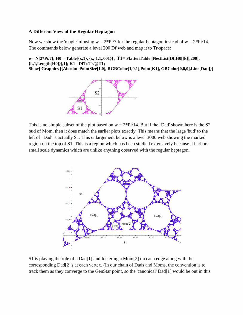
A Different View of the Regular Heptagon
Now we show the magic of using w = 2Pi7 for the regular heptagon instead of w = 2Pi14
The commands below generate a level 200 Df web and map it to Tr-space
w= N[2Pi7] H0 = Table[x1 x-11001] T1= FlattenTable [NestList[DfH0[[k]]200]
k1Length[H0]]1] K1= DfToTrT1
Show[ Graphics [AbsolutePointSize[10] RGBColor[101]Point[K1] GBColor[000]Line[Dad]]
This is no simple subset of the plot based on w = 2Pi14 But if the lsquoDad shown here is the S2
bud of Mom then it does match the earlier plots exactly This means that the large bud to the
left of Dad is actually S1 This enlargement below is a level 3000 web showing the marked
region on the top of S1 This is a region which has been studied extensively because it harbors
small scale dynamics which are unlike anything observed with the regular heptagon
S1 is playing the role of a Dad[1] and fostering a Mom[2] on each edge along with the
corresponding Dad[2]s at each vertex (In our chain of Dads and Moms the convention is to
track them as they converge to the GenStar point so the canonical Dad[1] would be out in this
region S1 is identical to Dad[1] except he is located in the inner star region as shown
aboveThis means his local dynamics are quite different from the canonical Dad[1])
The central Mom[2] shown above has radius GenScale2 so she should be the matriarch of a
normal generation 3 family - which is self-similar to generation 1 In the vertical direction the
dynamics are fairly normal But the remaining dynamics around Mom[2] are far from normal
She has the correct S2 buds but no S1 buds This is due to the influence of the large S2 on the
left The S1 and S2 scales do not have a common ground
Every prime regular polygon has Floor[N2] scales - one of which is the identity scale So
starting with N = 7 there are at least 2 non-trivial scales Typically these scales are non-
commensurate so they combine to generate an infinite array of possible sub-scales For example
there could be a Mom who is 4th generation S2 and third generation S1 Her radius would be
scale[2]4GenScale
3 Buds like this do occur and the corresponding dynamics are unlike anything
from previous generations Also the order in which generations evolve is critical so two Moms
with identical size may have very different dynamics
The S2 buds on the right and left of Mom[2] are attempting to foster their own families - but
these families are the wrong size for this S1 environment Below are vector plots of Mom[2] and
Dad[2] They are normal size for second generation The S2 next to Mom[2] is also normal
size for a third generation S2 so his radius is rS2GenScale2
MomS2[3] is not directly related to either Mom[2] or Dad[2] Instead she is the matching Mom
for S2[3] so her radius is GenScale3scale[2] She is the first of her kind to appear and she is the
wrong size to be in this environment Note that she is not in any of the step-regions of Dad[2]
so her dynamics are not compatible with his The virtual S2[3] shown here would be her normal
left-side Dad He is drawn here because he shares an important vertex with Dad[2] and his
progeny are quite real as shown below (It is not unusual for virtual buds to have real progeny)
The plot below shows a portion of MomS2[3] on the right On the far left we can see that Dad[2]
is sheltering a normal-looking family But this is an S2 family with patriarch who is a fourth
generation DadS2[4] His position and size are correct relative the virtual S2[3] shown above but
they are totally out of place under Dad[2] ndash which should have a Mom[3] in the center of this
edge
This S2 generation under the edge of an S1 Dad is the source of the very complex dynamics
Note that there are 6 more DadS2[4]s in this region Four of these are where they should be - on
the edges of MomS2[3] or adjacent to the original DadS2[4] The two central buds are
lsquovolunteersrsquo which are totally out of placeThe dynamics surrounding Dad[4] are unlike anything
which has been observed before but the fact that there is a PortalMom[2] at the edge of this
region seems to imply that the dynamics are related to the dynamics of the even generations ndash
which are dominated by Portal Moms
The vector diagram below shows that Dad[4] does have some connections with the large
DadS2[4]rsquos which dominate this region We have drawn two virtual Dad[4]rsquos showing their fit
between the large buds at top and bottom In addition a virtual MomS2[4] fits very nicely and
shares some of her buds with the DadS2[4]rsquos
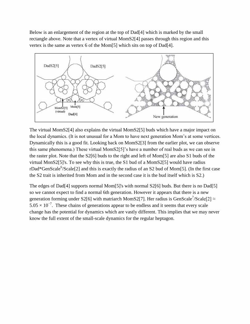
Below is an enlargement of the region at the top of Dad[4] which is marked by the small
rectangle above Note that a vertex of virtual MomS2[4] passes through this region and this
vertex is the same as vertex 6 of the Mom[5] which sits on top of Dad[4]
The virtual MomS2[4] also explains the virtual MomS2[5] buds which have a major impact on
the local dynamics (It is not unusual for a Mom to have next generation Momrsquos at some vertices
Dynamically this is a good fit Looking back on MomS2[3] from the earlier plot we can observe
this same phenomena) These virtual MomS2[5]rsquos have a number of real buds as we can see in
the raster plot Note that the S2[6] buds to the right and left of Mom[5] are also S1 buds of the
virtual MonS2[5]s To see why this is true the S1 bud of a MomS2[5] would have radius
rDadGenScale6Scale[2] and this is exactly the radius of an S2 bud of Mom[5] (In the first case
the S2 trait is inherited from Mom and in the second case it is the bud itself which is S2)
The edges of Dad[4] supports normal Mom[5]s with normal S2[6] buds But there is no Dad[5]
so we cannot expect to find a normal 6th generation However it appears that there is a new
generation forming under S2[6] with matriarch MomS2[7] Her radius is GenScale7Scale[2] asymp
505 times 10minus7
These chains of generations appear to be endless and it seems that every scale
change has the potential for dynamics which are vastly different This implies that we may never
know the full extent of the small-scale dynamics for the regular heptagon
The demarcation line in the raster plot marks the boundaries of an invariant region that partially
surrounds Dad[4] The opposite side of this boundary has very different (and equally bizarre)
dynamics These dynamics envelope PortalMom[2] as shown below
The Regular 9-gon
Below is a portion of a Df plot for N = 9 (using N = 18)
w= 2Pi18 DfWeb = Flatten[Table[NestList[DfH0[[k]]200] k1Length[H0]1]
TsWeb = DfToTsDfWeb
On the left below is the canonical First Family for N = 9 but the actual family contains two
lsquomutationsrsquo caused by the extra factor of 3 These mutations are shown in blue on the right side
S[3] (Step-3) would normally be a regular 18-gon but instead it is a non-regular 12-gon
composed to two interwoven hexagons with slightly different radii DS[3] (Dad-step-3) would
normally be a regular 9-gon and instead the sides are extended to form a non regular hexagon
Below is an enlargement of S[3] showing the two regular hexagons with slightly different radii
We call these woven polygons They are a natural occurrences for regular N-gons with N
composite
Below is a level 10000 web from Df showing the 2
nd generation under Dad There is a normal
Mom[1] and Dad[1] but no S[3]s or S[1]rsquos The gaps left by the S[3]rsquos is filled by four 9-gon
buds which have lsquohalosrsquo caused by the breakdown of the 18-gon S[3]rsquos into 9-gons Dad[1]
shelters a small 3rd
generation which appears to be self-similar to this 2nd
generation
Section 2 Digital Filters in Three Dimensions
Chua amp Lin [C2] describe a third order Df filter that showed dynamics similar to Df but in three
dimensions The circuit diagram is given below
The difference equation for the output is y(t+3) = f [ -a3y(t) - a2y(t+1) -a2y(t+2) + u(t+3)]
where u(t+3) is the input If we assume that the accumulator is in 2s complement form f is
unchanged from the second-order case Since we are once again interested in self-sustaining
oscillations set u(t) = 0 for all t The output equation can be reduced to three first order equations
by setting
x1 = y(t) x2 = y(t+1) x3 = y(t+2) Then at each time tick x1 rarrx2 x2 rarr x3 and x3 rarr f [ -a3x1 -
a2x2 - a1x3] The linear system is
X(k+1) = AX(k) where
1
2
3 3 2 1
0 1 0
and 0 0 1
x
x
x a a a
X A
with characteristic equation λ3 + a1λ
2 + a2λ + a3 = 0
Setting -(a+c) = a1 ac-b = a2 and bc = a3 this can be factored as (λ -c)(λ2 -aλ - b) in which case
the stable region is |c| le 1 |b| le 1 |a| le 1-b
Choose c and b values from the boundary c = 1 b = -1 then |a| lt 2 and a is the lone parameter
The linear evolution matrix is now 0 1 0
0 0 1
1 (1 ) 1a a
A
The full non-linear system is D3f[x_ y_ z_] = f[y] f[z] f[x - (1 + a)y + (1 + a)z]
with f[x_] = Mod[x + 1 2] - 1 as with Df Once again we assume that y and z are in range and
the angular variable corresponding to a is 2Cos[w]
D3f[x_ y_ z_] = y z f[x - (1 + a)y + (1 + a)z]
Just as with Df the system equations can be written to make the kicks explicit
1
1
1
0 1 0 0
0 0 1 0
1 (1 ) 1 2
k k
k k k
k k
x x
y y s
z a a z
For a given initial point x0y0z0 the sequence sk can be found by tracking its orbit with D3f
but now there are 7 possible values of sk 0 plusmn1 plusmn2 plusmn3 This is because the orbit of x0y0z0
may visit as many as 4 planes We will give Mathematica code below for finding the s-sequence
of any point
D3f is a map on the unit cube to itselfThe dynamics of the linear system lie in an ellipse as in
the Df case Evaluating the Jacobian the three eigenvalues 1 eiθ
e-iθ
have unit value except when
|x1 - (1+a)x2 + (1+a)x3| is odd (1357) The mapping is area preserving except for these
discontinuities
To see the dynamics of the linear map set f[x_]= x and try w = 10 so a = 2Cos[1] asymp 10816
Orbit=NestList[D3fx1001000] ListPointPlot3D[Orbit]
This ellipse can be aligned with the x1 = 0 plane usingT3 =
1 1 0
0
1
Cos Sin
Cos Sin
T3[w_] = 1 1 0 1 Cos[w] Sin[w] 1 Cos[2w] Sin[2w]
D3fToTr[q_] =Inverse[T3[w]]q ROrbit = D3fToTrOrbit ListPointPlot3D[Orbit]
Now we can project this onto the x2 x3 plane P23=Drop[ROrbitNone1] (this drops no rows
and the first column) ListPlot[P23 AspectRatio-gtAutomatic]
0
1
20
1
2
0
1
2
00
05
10
15
20
1
0
1
1
0
1
Below is the orbit of this same initial point 100 but with normal non-linear overflow
function f[x_]= Mod[x + 1 2] - 1 O ROrbit =
D3fToTrOrbit P23=Drop[ROrbitNone1] ListPlot[P23] Graphics3D[Point[Orbit]]
Points jump back and forth between the two planes but not necessarily in strict alternation
as above The first 4 points in the orbit of 100 are shown in pink In the x2x3 projection on
the left the arrow shows the initial point This is D3fToTr[100]=108767 -00876713-
123629 but with the first co-ordinate dropped In the 3D plot the points are the actual orbit so
the initial point shown is 100 (lower right)
The planes are parallel at distance 2Sqrt[2+a2 ] asymp 11237 This is the magnitude of a kick for a
=2Cos[1] So what we are seeing are the kicks from the s-sequence of this orbit Chua gives
the change of co-ordinates that can be used to restrict the map to these planes In this manner the
3 dimensional dynamics can be analyzed using the same techniques as the 2 dimensional case
Here is an example using the orbit above The new (orthogonal) basis vectors depend on the
parameter a e1 = (1Sqrt[2 + a^2])1 - a 1 e2 = (1Sqrt[2])1 0 -1 e3 = (1Sqrt[4 + 2a^2])a 2 a
These will be the columns of the transformation matrix T = Transpose[e1 e2 e3]
MatrixForm[T] = 2 2
2 2
2 2
1 1
22 4 2
20
2 4 2
1 1
22 4 2
a
a a
a
a a
a
a a
TI = Inverse[T]
10 05 05 10
10
05
05
10
O ut[1 6 0]=
The corresponding D3f map in T-space can be decomposed into two maps - one for the transport
between planes and one for the dynamics within the planes The first co-ordinate of the T-space
map tracks the jumps between the planes and since these coordinates are orthogonal the jump
distance is plusmn 2Sqrt[2+a2 ] This means that the first coordinate has the form uk+1 = uk +
2Sqrt[2+a2 ]s
For two planes the possible values of s are 01-1 Our current a value is 2Cos[1] asymp 10816
which is slightly larger than 1 so there may be as many as four planes and this means the
possible values for the s-sequence are0 plusmn1 plusmn2 plusmn3 There actually are 2 more small planes in
this example but they dont show up until after 25000 iterations They account for two of the
missing vertices of the triangles above We will plot them shortly but for now the dynamics are
restricted to just the 2 planes shown above
Example Using 100 as the initial point we will use the T-space map to find the first few
terms in the s-sequence The first step is to find the T-space point corresponding to 100
TI100 =0561859 0707107 0429318 so the first coordinate is u = 561859 Now
advance the orbit by one iteration and repeat D3f[100] = 0 0 -1 TI00-1 = -0561859
0707107 -429318 Note that the difference between the first coordinates is the distance
between the planes so u1 = u0 + 2Sqrt[2+a2 ]s where s = -1 D3f[00-1=0 -1 -00806046
and TI[] = 0561859 00569961 -0829194 so the s-sequence so far is -11 These are
the kicks that we see above
After 10000 iterations the orbit is still confined to these two planes but there are occasional
occurrences of 0 in the s-sequence For example the 10000th iterate of 100 is p0=
Last[Orbit] =-0100544-009348650999522 and if we track this point for 10 more iterations
we get a mapping from the lower plane to itself as shown below These become much more
common as the complexity increases
The dynamics of 100 are very complex and it is likely that this orbit is non-periodic But the
initial dynamics follow a simple pattern of rotation around the ellipses (which are circles above
in the rectified plot) and gradually the points move outwards toward the vertices of the triangles
It is there that the 3-dimensional dynamics overflow the boundaries of the unit cube and two
more small planes are needed to contain the tips (The worst case scenario of this overflow and
cropping explains why 4 planes suffice for any dynamics)
The overflow into planes 3 and 4 is just visible below on the projections and the corresponding
3D plot
Orbit=NestList[D3f10030000]ROrbit=D3fToTrOrbitP23=Drop[ROrbitNone1]
ListPlot[P23] Graphics3D[Point[Orbit]]
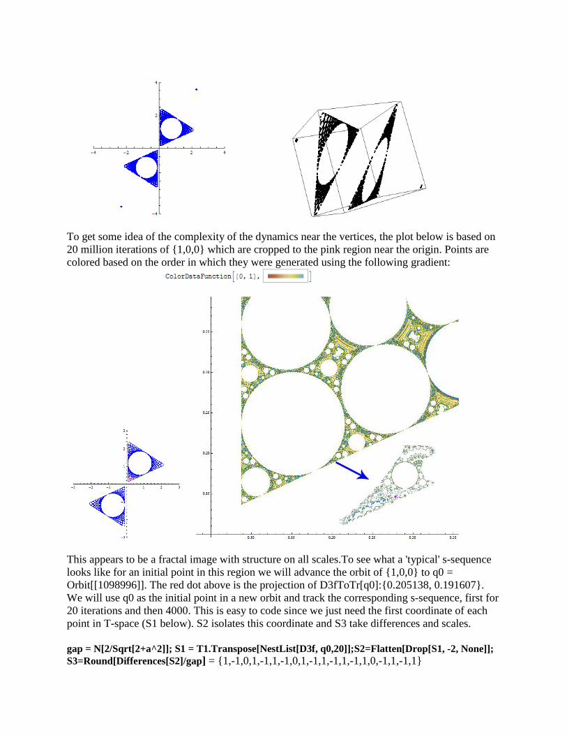
To get some idea of the complexity of the dynamics near the vertices the plot below is based on
20 million iterations of 100 which are cropped to the pink region near the origin Points are
colored based on the order in which they were generated using the following gradient
This appears to be a fractal image with structure on all scalesTo see what a typical s-sequence
looks like for an initial point in this region we will advance the orbit of 100 to q0 =
Orbit[[1098996]] The red dot above is the projection of D3fToTr[q0]0205138 0191607
We will use q0 as the initial point in a new orbit and track the corresponding s-sequence first for
20 iterations and then 4000 This is easy to code since we just need the first coordinate of each
point in T-space (S1 below) S2 isolates this coordinate and S3 take differences and scales
gap = N[2Sqrt[2+a^2]] S1 = T1Transpose[NestList[D3f q020]]S2=Flatten[Drop[S1 -2 None]]
S3=Round[Differences[S2]gap] = 1-101-11-101-11-11-110-11-11
For longer sequences the Tally command will keep track of the jumps The larger jumps begin
after 3234 iterations
S1 = T1Transpose[NestList[D3f q0 4000]] S2=Flatten[Drop[S1 -2 None]]
S3=Round[Differences[S2]gap] Tally[S3] = 11762-117610420-25325
-32423
Below is the tally for 2 million iterations with initial point 100
-192046919204680152415-264832676-326762648
This is the type of tally we would expect from a periodic orbit or from a non-periodic orbit which
is quasi-periodic in the sense that it is the limit of periodic orbits (as in the regular pentagon)
For the Df map a given value for the angular parameters a determined the dynamics- which
essential take place on 2 planes With D3f it comes as no surprise that a given value of a
determines an infinite range of possible dynamics For a fixed a value every u value will yield a
different set of planes For |a| lt 1 there are 2 or 3 planes and otherwise 3 or 4 For a given u
Chua defines I2
u to be the union of these planes Two sets of planes I2
u and I2
v cannot intersect
unless u =v Since the D3f map is invariant on each I2
u it is possible to use information about 2-
dimensional dynamics to analyze the dynamics of D3f But the diversity of possible dynamics is
staggering
If we were to keep a fixed in the example above and change the initial point even the smallest
change could lead to totally different dynamics There is no simple measure of distance which
will tell us which points are close to 100 in D3f space
For the Tangent map with a parameter such as w = 2Pi14 we are left with an infinite array of
possible I2
u dynamics to consider Hopefully one of these will mimic the perfect dynamics of
the Df map
Section 3 Dynamics of an Analog to Digital Converter
Investigators such as Orla Feely [F] have found qualitatively similar behavior between Df
dynamics with those of a second order bandpass Delta-Sigma modulator These modulators are
used in Analog to Digital conversion A typical block diagram for a (first order) ADC is show
below
The input is analog voltage and the output is a digital pulse stream with constant amplitude The
interval between pulses is determined by the primary feedback loop A low input voltage
produces longer intervals between pulses (and hence a smaller count in the Sigma counter) The
Delta pulse zeros out the integrator to get ready for the next integration The Sigma counter
counts the pulses over a given summing interval dt
The first order ADC has stable behavior for all inputs which are in range but this is not the case
for the second -order ADC shown below It has two integrators and hence 2 feedback loops
This type of negative feedback is common in biology economics as well as mechanical systems
In biology it is known as homeostasis and in mechanical systems it may be an attractor or an
equilibrium state In chemistry it is not unusual for one set of chemical signals to oppose
another Often these opposing forces are non-linear
The non-linearity in the ADC is due to the one-bit DAC which can be modeled with a sign
function
1 0
sgn 0 0
1 0
if x
x if x
if x
The input-output equations for the ADC as formulated by Feeley and Fitzgerald has the form of
a second order difference equation
2 2
2 1 1 12 cos 2 cos ( sgn ) ( sgn )k k k k k k ky r y r y r x y r x y
where x is the input y is the output r is the gain and θ is a parameter that is chosen to center the
filter at the desired sampling frequency (High frequency signals must be sampled at higher rates
For MP3 music the user can select the sampling rate - but the higher the rate the more memory is
needed)
In numerical studies we will set the gain r = 1 and to obtain self-sustaining behavior set x = 0
This reduces the above difference equation to
2 1 12cos ( sgn ) ( sgn )k k k k ky y y y y
Set x1 = yk and x2 = yk+1 then at each time tick x1 rarrx2 and x2 rarr 2cosθ(x2 - sgnx2) - (x1-sgnx1)
In matrix form
1
1
00 1
sgn 2cos sgn1 2cos
k k
k k k k
x x
y y x y
Note that the 2 by 2 linear matrix A above is identical to the Df matrix with b = -1 and a =
2Cosθ A is conjugate it to a simple rotation using DfToTr from Section 1
In Mathematica Adc[x_y_]=y 2Cos[w](y - Sign[y]) - (x - Sign[x])
Example a = 2Cos[w] = -8 Orbit = NestList[Adc 001 0 100000]
To track the regular pentagon set w = N[2Pi5] and again pick an initial point close to the
origin q1 = -001001 Rectify these points using
TrOrbit = DfToTrOrbit
We can fill in the gaps by taking the union of this map with its reflection obtained by swapping x
amp y This is shown on the right above in blue overlaid on top of the original map Even though
Adc is globally defined it is only invertible on two trapezoids which are a function of θ These
trapezoids can be see above for θ= ArcCos[-4] asymp 198231 and θ = 2π5 but one condition for
invertibility is that θ ge π3 so N = 5 is the last regular polygon that can be modeled However we
will see in Section 6 that a Harmonic Kicked Oscillator yields a map which is locally conjugate
to Adc and invertible for almost all θ This map continues the chain of conjugacies back to the
Tangent Map
Section 4 Hamiltonian Dynamics
From the perspective of Hamiltonian dynamics the digital filter map and ADC maps are
examples of kicked Hamiltonians
The Hamiltonian of a physical system is a function of (generalized) position q and
(generalized) momentum p In some cases it may change in time so it is writen as
( ( ) ( ) )i iH q t p t t where i = 1N are the degrees of freedom of the physical system The
dynamics of a Hamiltonian system are given by
i i
i i
H Hq p
p q
So a Hamiltonian system is a system of differential equations which are related by H Not every
system of differential equations has a corresponding Hamiltonian When H does not depend
explicitly on time the state of the system at any given time is a point (piqi) in 2N-dimensional
space phase space The motion of this point is determined by the equations above Starting with
an initial set of points the volume will be preserved over time because the equations above
imply that H is conserved 0i i
i i
dp dqdH H H
dt p dt q dt
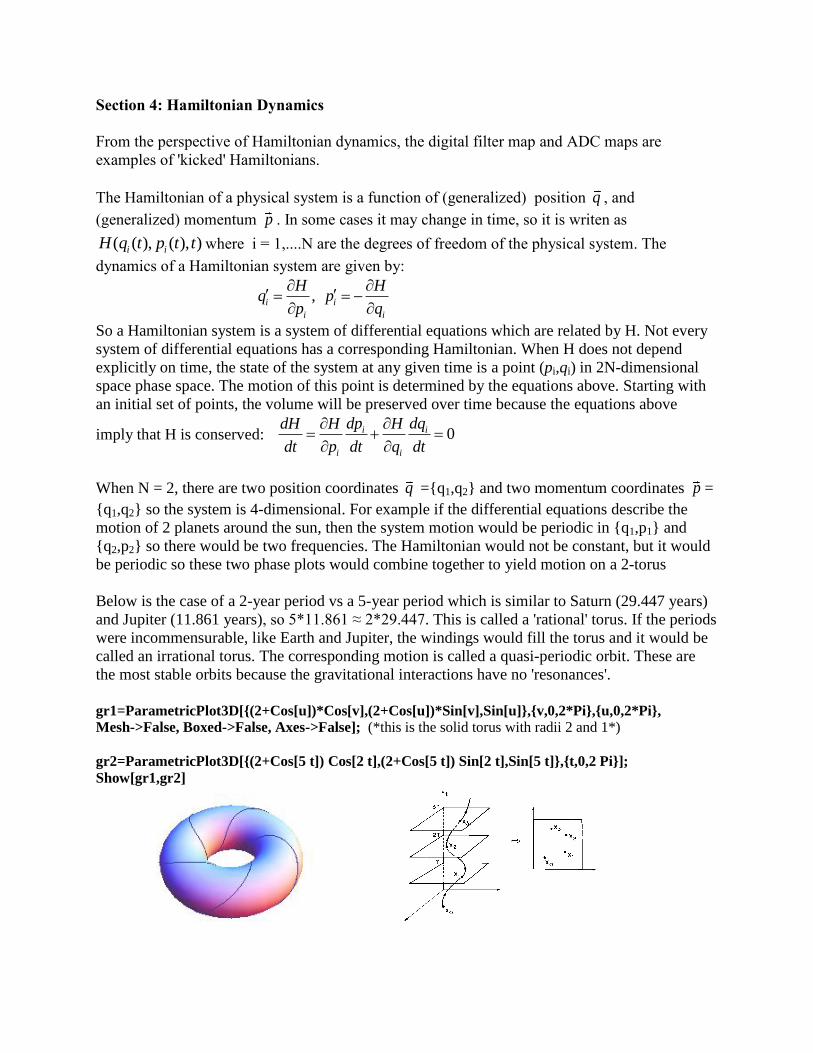
When N = 2 there are two position coordinates q =q1q2 and two momentum coordinates p =
q1q2 so the system is 4-dimensional For example if the differential equations describe the
motion of 2 planets around the sun then the system motion would be periodic in q1p1 and
q2p2 so there would be two frequencies The Hamiltonian would not be constant but it would
be periodic so these two phase plots would combine together to yield motion on a 2-torus
Below is the case of a 2-year period vs a 5-year period which is similar to Saturn (29447 years)
and Jupiter (11861 years) so 511861 asymp 229447 This is called a rational torus If the periods
were incommensurable like Earth and Jupiter the windings would fill the torus and it would be
called an irrational torus The corresponding motion is called a quasi-periodic orbit These are
the most stable orbits because the gravitational interactions have no resonances
gr1=ParametricPlot3D[(2+Cos[u])Cos[v](2+Cos[u])Sin[v]Sin[u]v02Piu02Pi
Mesh-gtFalse Boxed-gtFalse Axes-gtFalse] (this is the solid torus with radii 2 and 1)
gr2=ParametricPlot3D[(2+Cos[5 t]) Cos[2 t](2+Cos[5 t]) Sin[2 t]Sin[5 t]t02 Pi]
Show[gr1gr2]
To reduce this motion to a 2-dimensional mapping choose a reference plane For example slice
the torus at a fixed longitude q0 and strobe the longer 5 year period with the shorter 2-year
period by setting δt = 2 years
These surfaces of section are also called Poincare return maps They can be used to help uncover
periodic motion or fixed pointsSince the system equations are differential equations continuity
would imply that orbits in the vicinity of a fixed point will behave in a predictable fashion based
on the Jacobian Because S is symplectic the Jacobian at any fixed point will have eigenvalues
of the form λ 1λ There are only three types of behavior possible near a fixed point
(i) λ positive and λ gt 1 (1λ lt 1) This is an unstable hyperbolic saddle point where the motion
expands in one direction and contracts in another
(ii) λ negative and |λ| gt1 (1|λ| lt1) Similar to (i) above but displacements in each direction vary
from positive to negative on each iteration
(iii) λ complex - in which case λ and 1λ must have zero real part so they have the form λ = eiθ
and 1λ = e-iθ
This is called a center or a neutral fixed point Nearby points will rotate by θ on
each iteration
Case (iii) is the only case where stability is not obvious because this marginally stable behavior
may be very sensitive to small perturbations This is the heart of the KAM Theorem How will
the marginally stable fixed points of a well-behaved Hamiltonian system react when subjected
to periodic perturbations (ie when gravity between Jupiter and Saturn is turned on) Will a
finite measure of the quasi-periodic orbits survive Is the solar system stable
Note that it is not possible for solutions to spiral into or away from a fixed point and also it is not
possible to have expansion without contraction These are consequences of the symplectic
property of the Hamiltonian
A 2-degree of freedom Hamiltonian such as the one above would be classified as well-behaved
or integrable if there are 2 integrals of motion A function f( p q ) is an Integrable of Motion if it
satisfies the Poisson bracket (commutator) relationship
[f H] = 0i i
i i
p qf f df
p t q t dt
Therefore an integral of motion is also a constant of motion The system energy H( p q ) is
always a constant of motion Note that the torus maps shown above have non-Eulidean metric
just like the raw Df maps We can obtain the integrals of motion by performing a canonical
change of variables to convert the map S into normal Euclidean form so that ellipses become
circles The new variables are called action-angle variables ( p q ) rarr ( )I In the new
surface of section map θ will represent a simple rotation The Is are the two constants of
motion
j
j
C
I p dq where the integral is around the jth axis of the torus
Example Two coupled oscillators with unit mass m 2 2 2 2 2 2
1 1 1 2 2 2
1 1( ) ( )
2 2H p q p q
where 1 1 2 2 and k k Transformation to action-angle variables yields
1 1 1 1 1 1 1 12 cos 2 sin p I q I and 2 2 2 2 2 2 2 22 cos 2 sin p I q I so the new
Hamiltonian is 1 1 2 2H I I and I1 and I2 are the integrals of motion
The motion is the same as 2 uncoupled oscillations 1 1 1 2 2 2( ) (0) and ( ) (0)t t t t so
the periods are 2πω1 and 2πω2 and the motion does not depend on the central spring
The KAM Theorem starts with an integrable Hamiltonian and asks what happens when it is
perturbed For the N = 2 case of Saturn and Jupiter this amounts to turning on the gravitational
attraction between them In this case the answer to the stability question depends largely on the
ratio of the periods A ratio such as 25 could be dangerous over long time periods because it
means that Saturn will feel systematic effects which could build up over time It is not clear
whether the canonical change of variables will remain meaningful under perturbations and the
new system will generally not be Integrable
The early solar system was a turbulent place and recent studies show that there may have been an
even more dangerous 21 resonance between Saturn and Jupiter in the early history of the solar
system This resonance might have caused Neptune and Uranus to migrate outwards and this in
turn would have created havoc among the millions of planetesimals in that region
If there is observable chaotic motion within our solar system currently it is probably in the orbits
of irregular satellites The first irregular satellite that has been imaged close-up and studied in
detail is Saturns Phoebe Recently there have been a number of new discoveries of irregular
satellites orbiting the four gas giants Jupiter Saturn Uranus and Neptune These discoveries
were made possible by attaching new wide-field CCD cameras to large telescopes
The Earth recently captured a small irregular asteroid It was called 2006 RH120 and it was about
15 meters wide It only survived for about 4 orbits before returning to its orbit around the sun
The dates were September 2006 to June 2007 Latest news is that there is another companion to
the Earth in an irregular orbit It is known as 2010 SO16
To see what happens to an integrable Hamiltonian when it is perturbed we will look at the case
of one degree of freedom H(θp) = ωp2 so the momentum p is constant The corresponding
Poincare return map is θk+1= θk + p so points rotate by a fixed amount pWhen the perturbation is
of the form Ksinθk this is called the Standard Map
The Standard Map
1
1
sin
sin
k k k k
k k k
x x y K x
y y K x
When x plays the role of the angular variable θ and y plays the role of momentum p The
determinant of the Jacobian is 1 so it is area preserving Since the perturbation is periodic
modulo 2Pi it is common to scale x and K by 2Pi and plot x Mod1 Following normal
convention we will plot both x and y Mod 1
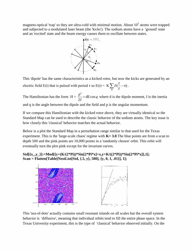
Std[x_ y_] = Mod[y + (K(2Pi))Sin[2Pix] + x y + K((2Pi))Sin[2Pix] 1]
Example K =0971635406 gamma = (Sqrt[5]-1)2
Orbit1= NestList[Std 0gamma 1000] Orbit2= NestList[Std 01-gamma 1000]
To get a range of initial conditions passing through the center of the plot
VerticalScan = Flatten[Table[NestList[Std 5 y 1000] y 0 1 01] 1]
Graphics[AbsolutePointSize[10]BluePoint[VerticalScan]Magenta Point[Orbit1]
Point[Orbit2]Axes-gtTrue]
This mapping is a paradigm for Hamiltonian chaos in the sense that it is an area preserving map
with divided phase space where integrable islands of stability are surround by a chaotic
component The two magenta orbits are remnants of the last surviving invariant torus - with
highly irrational winding number equal to the Golden Mean (See Section 8) As K increases past
0971635406 and these curves break down there is no further impediment to large scale chaos in
the central region
The K = 0 case corresponds to an integrable Hamiltonian such as H(θp) = ωp2 so the angular
momentum p is constant and the Standard Map reduces to a circle map (twist map) xk+1= xk + y
with winding number y The circles (tori) come in two varieties depending on whether y2π is
rational or irrational When K gt 0 The Standard Map simulates what happens to H when it is
perturbed by periodic kicks of the form sinK x So the Standard Map is a Poincare cross section
of perturbed twist map We will derive the equations below using a kicked rotor
The fixed points are at 00 and 120 The Jacobian is J = (
)
= 1 1
cos 2 1 cos 2K x K x
At 00 J =
1 1
1K K
so this is an unstable saddle point as
we can see above At 120 J = 1 1
1K K
and this is a center for (04)K
Therefore for K in this range the motion in the vicinity of 120 is locally conjugate to a
rotation These rotations are the cross sections of the tori from the Hamiltonian and we know
that the curves with irrational winding numbers (like the Golden Mean curve) are most likely to
survive as the perturbations are increased At this resolution it is hard to tell which curves are
rational and which are irrational Below is an enlargement of a central region showing the
nesting of rational and irrational curves
Moving outwards from the center means that the conjugacy may no longer be valid For small K
the set of surviving curves can be parameterized by a Cantor set so they form a continuum but
the regions between these irrational curves contains rational rotations with periodic orbits such as
the period 46 orbit above Under perturbations the KAM Theorem says that tori which are
sufficiently irrational will survive while most rational tori will break up into the resonant
islands that we see in the Standard map This process repeats itself at all scales as shown in the
drawing below The s are unstable saddle points which form between the islands Each
island represents a locally fixed point because periodic points of a mapping S are fixed points of
Sk
For small perturbations a finite measure of tori will survive and this guarantees stability The
invariant curves that do survive partition the phase space and limit the chaotic diffusion The
dark regions in the Standard map plot are the chaotic debris left over from the breakdown of
rational torus If an asteroid had these initial conditions it might be flung from its orbit
Deriving the Standard Map from a Kicked Rotor
Consider a pendulum allowed to rotate in zero gravity and subjected to periodic kicks of
magnitude K at time intervals τ as shown here
If this were an asteroid in orbit around the sun the kicks might be gravitational interaction with
Jupiter Another important scenario is a cyclotron where charged particles are accelerated to high
speed in a magnetic field created by an alternating electric field
The Hamiltonian is time dependent 2
( ) cos ( )2 n
pH p t K n
I
t
where I is the moment of inertia of the pendulum which we will scale to be 1 and is the Dirac
Delta function which yields pulses only when the input is 0 and this occurs at time intervals τ so
( ) ( )n
t K nt
is the periodic pulse stream shown above
From the Hamiltonianwe can see that the pulse stream alters the Potential Energy at periodic
intervals and this shows up in the system equations as a change in Kinetic Energy
The equations of motion are sin ( )n
dpK n
dt
t
and
dp
dt
So the rotor receives a periodic torque of magnitude Ksinθ at time intervals ∆t = τ For the
discrete equations we can scale the intervals to get τ = 1 The effect of the kth kick is to update p
based on the current value of θ so pk+1 = pk + Ksinθk Between kicks the motion is force free so
p is constant and the second equation above says that θ is updated by p∆t = p so θk+1= θk +
pk+1This gives the following equations which describe the system just after the kth kick
1 1
1
sin
sin sin
k k k k k k
k k k k k
p p K
p p K p K
These equations are identical to the Standard map and this tells us that the kicked rotor would
have very interesting dynamics but zero-gravity is hard to simulate in a lab We can see this
scenario being played out in celestial mechanics but the planetary time scale is typically very
long On a shorter scale we can the track the orbits of satellites or asteroids where the periodic
perturbations may be due to the irregular orbits or irregular shapes Particle accelerators and
fusion reactors live at a much faster pace and instabilities are a major issue in both cases
The Delta-Kicked Rotor in Quantum Physics
In quantum physics momentum P and position X are no longer independent They are related by
the Poisson commutation relationship [ ] where X P XP PX i = 2h is the reduced
Plank constant 341054571 10 joule seconds It represents the proportionality between the
momentum and quantum wavelength of a particle In 1926 Werner Heisenberg realized that this
commutation relationship implies that 2X P where and PX are deviations in the
measured values of position and momentum This is known as the Heisenberg Uncertainty
Principle It says that it is not possible to know both of these quantities with high accuracy at the
same time because decreasing one uncertainty increases the other This principle underlies all of
quantum mechanics and has wide-ranging implications
For large aggregates of atoms quantum effects can often be ignored and it is possible to apply
the classical laws of physics like Newtons laws of motion and the laws of electricity and
magnetism The dividing line between the classical and quantum worlds is very difficult to
determine and recently there have been studies showing that quantum affects can be observed all
around us if we look carefully Often these effects are in conflict with the laws of classical
physics
No one doubts that the laws of quantum mechanics govern the behavior of particles on very
small scales but some of these laws seem very bizarre and they do not seem to apply to the
macro world around us The laws of classical physics should be based on these quantum laws
but no one knows how to do this - so we formulate approximations and call these the laws of
physics
Vlatok Vedral describes an example involving ordinary salt On the left below are random
orientation of molecules in a salt crystalWhen a magnetic field is applied the atoms have a
tendency to align themselves with the field but in fact they align themselves much more
efficiently than the classical prediction Physicists believe that this is due to quantum effects
which predict that at a certain scale and energy level particles have a natural entanglement
In Moore et al a group of five physicists at the University of Texas used ultra-cold salt atoms in
an experiment which showed a similar entanglement The first step was to trap the atoms in a
magneto-optical trap so they are ultra-cold with minimal motion About 105 atoms were trapped
and subjected to a modulated laser beam (the kicks) The sodium atoms have a ground state
and an excited state and the beam energy causes them to oscillate between states
This dipole has the same characteristics as a kicked rotor but now the kicks are generated by an
electric field E(t) that is pulsed with period τ so E(t) = K ( )n
nt
The Hamiltonian has the form H = 2
dEcos2
pq
I where d is the dipole moment I is the inertia
and q is the angle between the dipole and the field and p is the angular momentum
If we compare this Hamiltonian with the kicked rotor above they are virtually identical so the
Standard Map can be used to describe the classic behavior of the sodium atoms The key issue is
how closely this classical behavior matches the actual behavior
Below is a plot the Standard Map in a perturbation range similar to that used for the Texas
experiment This is the large-scale chaos regime with K= 30 The blue points are from a scan to
depth 500 and the pink points are 10000 points in a randomly chosen orbit This orbit will
eventually turn the plot pink except for the invariant curves
Std[x_y_]=Mod[y+(K(2Pi))Sin[2Pix]+xy+K((2Pi))Sin[2Pix]1]
Scan = Flatten[Table[NestList[Std 5 y 500] y 0 1 01] 1]
This sea-of-dots actually contains small resonant islands on all scales but the overall system
behavior is diffusive meaning that individual orbits tend to fill the entire phase space In the
Texas University experiment this is the type of classical behavior observed initially On the
right above is a plot of their results The solid line is the classical prediction of the energy gain as
the sodium atoms are pulsed This corresponds closely to behavior predicted by the delta-kicked
rotor and illustrated above by the Standard Map The x-axis of their plot is the number of cycles
of pulsing and refreezing After about 8 cycles there was significant drop-off of energy This
drop-off is due to a quantum effect called localization and it had been predicted by theory and
by earlier experiments This behavior appears to be related to the magnetic induced
entangelment found in the salt crystals
As indicated earlier the classical kicked rotor (and the resulting Standard Map) are regarded by
physicists as paradigms for Hamiltonian chaos but this is the first time that this behavior was
controlled in a laboratory so that it was possible to observe the transition between classical and
quantum dynamics
For any discrete mapping to be of value in quantum mechanics it has allow for a consistent
quantization The Standard Map allows researchers to impose this quantization and the same is
true for thee kicked Harper Map which we will examine in Section 6
Section 5 The Sawtooth Standard Map
The non-linearities with Df and D3f arose from discontinuities in the overflow function f[x_]=
Mod[x + 12] - 1 and the non-linearities of the Adc map arose from one-bit discontinuities
modeled with x-Sign[x] These are both examples of sawtooth maps which in Mathematica are
called SawtoothWave functions SawtoothWave[x] is defined to be x-Floor[x]
There have been a number of studies done with the Standard Map by replacing the kick function
( ) sin 2f x x with either non-analytic or non-smooth functions Usually the non-smooth
functions are piecewise linear sawtooth maps For example VV Vecheslavov has studied the
dynamics of the following piecewise version of ( ) sin 2f x x
Saw[x_]=Which[ lt=25 4x Abs[5-x]lt=25 4(5-x) Abs[x-10]lt=25 4(x-1)]
Plot[ Saw[x] x01]
2 1 1 2
10
05
05
10
Mod x 12 1
2 1 1 2
10
05
05
10
x Sign x
2 1 1 2
02
04
06
08
10
SawtoothWave x
The corresponding SawtoothSine Standard Map is
1
1 1
KSaw( )k k k
k k k
p p x
x x p
SawSine[x_ y_] = Mod[x + KSaw[y] 1] Mod[x + KSaw[y] + y 1]
For some K values this map is similar to the Standard Map but for most values of K the
dynamics are quite different - especially near resonant values such as K = 13 and K = 18
Below are three sample plots using K =2Cos[2Pi14] - 2 K = 332 and K = 12
IC Percival and others have studied families of Sawtooth maps obtained by linearizing the
Standard Map about the stable fixed point at 120 These map have the form
1
1 1
( 1 2)k k k
k k k
p p K x
x x p
Where only x is taken Mod 1 so it maps the cylinder [01) to itself The kick function
( ) sin 2f x x of the Standard Map is replaced with ( ) ( 1 2) Mod1f x x
Plot[Mod[x-121]x01Exclusions-gtNone ]
The discontinuity at x = 12 destroys the stable fixed point at 120 (except for integer values
of K-in which case it is a cat map) yielding a map which is everywhere hyperbolic The
divided phase space of the Standard Map is often not desirable in transport problems which
arise for example in fusion reactors This is an example of an Anasov map There is a more
benign version of this map which preserves the stable fixed point to retain a phase space which
contains both regular and chaotic dynamicsThis is what Peter Ashwin calls the Sawtooth
Standard Map The corresponding sawtooth map is S
On the interval [01] Saw[Saw[x]] = x - 12 Below is the (inverted) Standard Map and the
Sawtooth Standard Map (both are Mod 1)
1
1
sin 22
sin 22
k kk
kk k k
Kx y
x
y Ky x y
1
1
( )
( )
k k k
k k k k
x x kSaw y
y y x kSaw y
For the (inverted) Standard Map the Jacobian is
J = (
) = 1 cos 2
1 1 cos 2
K y
K y
so at 012 J =
1
1 1
K
K
The Sawtooth map also has a fixed point at 012 and the Jacobian is 1
1 1
k
k
so k = -K relative to the Standard Map Note that (unlike the Standard Map) the Jacobian is
constant In both cases Det[J] = 1 so they are area preserving (symplectic) This implies that the
eigenvalues come in pairs λ1 1λ1) Here λ1 =1
(2 4 )2
k k k The eigenvalues are
complex for [ 40]k In this range the eigenvalues have the form ie
where θ is given by
2cos 2k so we can use either k or θ as the parameter of the map The range for θ is [0 π]
which is perfect for regular polygons Using the Saw function defined above the Sawtooth
Standard Map is StSaw[x_ y_] = Mod[x + kSaw[y] 1] Mod[x + kSaw[y] + y 1]
Peter Ashwin [AP] showed that this map is equivalent to the Df map via a linear change of
coordinates We will give details below As with Df the web for a regular N-gon can be obtained
using θ = 2Pi2N not 2PiN
Example k = N[2Cos[2Pi14]-2] The following plot generates a web by scanning the x axis
from 0 to 1 at depth 1000
Below are the first 3 iterations of the web overlayed on the above plot
XAxis = Table[x 0 x 0 1 001]
Just like Df these webs are perfect matches for the Tangent Map webs but the dynamics are
different To map StSaw space to Tr space for the Tangent Map we will use Peter Ashwins
linear transformation from StSaw to Df-space and then use DfToTr Here is an example
The canonical remainder function is r[x] = x - Floor[x] (which is also SawtoothWave[x]]
Using this function the change of coordinates from xy in StSaw to uv in Df is
2 ( ) 1
1 2
u r x y
v y
In Mathematica StSawToDf[x_ y_] = 2r[x - y] - 1 1 - 2y
Example θ= 2Pi14 so k = N[2Cos[2Pi14] - 2] as above
DfWeb =StSawToDfStSawWeb TrWeb = DfToTrDfWeb
Below is StSawWeb in pink DfWeb in blue and TrWeb in black All these maps are invertible
This shows a rather remarkable chain of conjugacies which has its roots in the Standard Map
which is special case of a general Kicked Map where the kicks are applied relative to the
position coordinate q but they alter the momentum coordinate p
1
1 1
( )k k k
k k k
p p Kf q
q q p
The sawtooth maps replace the Standard Map kick function ( ) sin 2f q q with piecewise
linear functions Jurgen Moser proposed the Tangent Map for the same reason - to see what
happens to the KAM Theorem when the smoothness of the perturbation function is violated
The story of why Moser chose to make smoothness assumptions rather than the analytic
assumptions used by the Russians is interesting - both from a historical perspective and a
mathematical perspective Because of the Iron Curtain there was very limited exchange of
information In the end the Russians though Mosers approach was superior (because real
analytic functions are a proper subset of smooth functions) but Moser felt that Kolmogorovs
insights were the key element in the KAM Theorem In 1971 Moser [JM2] wrote a textbook on
the subject explaining both approaches
In his original version of the lsquoTwist Theoremrsquo Moser needed to assume a function with 333
continuous derivatives (C333
) but this was later refined by Russman to a C5 curve and Moser
conjectured that it even may hold for C2 Counterexamples exist for the C
1 case (FTakens -
1971) The Tangent Map and piecewise linear maps are neither analytic nor C1 so they can be
used as testing grounds to see what happens when the KAM Theorem breaks down
Section 6 The Kicked Harmonic Oscillator (KHO)
The Standard Map is based on a kicked rotor in zero gravity so there is no natural frequency of
rotation for the unperturbed system - it is a free rotor whose frequency is determined by the
initial conditions The KHO is based on a harmonic oscillator so it mimics the linear pendulum
with gravity turned on Now there is a natural frequency of oscillation (ω0 ) which depends on
the length for the pendulum or the spring constant for the oscillator shown below
KE = 2 2
21 ( )
2 2 2
mv pmv
m m where v is x The PE depends on the spring constant k Hooks law
says that (for small vibrations and a soft spring) the restoring force on the spring is proportional
to the displacement so F = kω0x for a constant k
The Hamiltonian is 2 2 2
2
0 0 and m can be scaled to get 2 2 2
p p xk x
m
The kicked system has the form H = 2 2
0 ( )2 2 n
p x tV x n
where the kicking
potental V(x) is usually of the form cos or sinkxkx (even or odd)
In quantum mechanics KHOs have been used to model the behavior of charges in a uniform
magnetic field subject to periodic kicks electronic transport in semiconductor lattices or
cyclotron resonance where a resonant particle (0
2n
) will experience continuous
acceleration Typically the even and odd cases have very different dynamics Below is an
example of an even potential
Using V(x) = 0 cosK
x
the Hamiltonian is
2 2 2 00
1( ) cos
2 n
w K tp x x n
which reduces to the Standard map when ω0rarr0 Krarrinfin and ω0K = constant
The discrete version is sometimes called the (stochastic) WebMap
1
1
sincos sin
sin cos
k k k
k k
u u K v
v v
where u = xω0 v = x and α = ηω0 The linear form of this map is the unperturbed harmonic
oscillator which yields simple rotation in phase space so between kicks the particle rotates
clockwise by α For certain parameter values the Web Map models particle motion in a constant
magnetic field
In generic xy form the equations are
KHO[x_ y_] = (x + KSin[y])Cos[w] + ySin[w] -(x + KSin[y])Sin[w] + yCos[w]
Example K = 15 w = 2Pi4 H2 = Table[x x x -6 6 0374]
T1 = Flatten[Table[NestList[KHO H2[[k]] 1000] k 1 Length[H2]] 1]
Since w = α = ηω0 = 2π4 the plot above represents a 14 resonance between the kick frequency
(ωk= 2πη) and the resonant frequency ω0 It is the ratio of these frequencies which determines
the global behavior of the system For the Tangent Map the case α = 2π4 corresponds to the
square N = 4 In this case the web tiles the plane with congruent squares (or rectangles) as we see
above This is called 4-fold symmetry The cases for α = 2π3 ( N= 3) and α = 2π6 (N = 6) also
tile the plane in a regular fashion Actually these two tilings are congruent
The KHO map for the regular pentagon N = 5 ( α = 2π5 K = 15) is shown below This is a
quasi-crystalline structure which shows less robust diffusion than N=346 The right side is the
corresponding Tangent Map for N = 5 showing the rings of Dads which confine the dynamics
The N = 1 and N = 2 cases are degenerate lattices which correspond to operating regimes of the
early cyclotrons For other integer N values the structure is quasi crystalline and the
corresponding quantum evolution show initial suppression of diffusion - until K is large enough
to allow tunneling For irrational ratios all traces of crystalline structure disappear but there is
still diffusion at high energy levels This case corresponds to a Tangent Map on a circle or ellipse
and all orbits are also circles or ellipses with no intervening channels
In quantum mechanics the most important cases are N = 3 4 and 6 because the corresponding
tiles represent extended quantum eigenstates and the channels allow diffusion over time so they
are testing grounds for quantum delocalization- of the type observed in the cold-atom
experiments The classical model of diffusion over time is nearly linear as shown below while
the quantum model shows sharp drop-off due to delocalization
Once again we note that the maps shown here only simulate the classical predictions To track
the quantum evolution of the system it is necessary to generate time-dependent waveforms -
usually with the aid of Fractional Fourier Transforms
Over the past 15 years many laboratories world-wide have replicated the Texas University cold-
atom experiments showing this drop-off at the classical-quantum transition Experiments have
advanced from cold-atoms to more robust Boise-Einstein condensates But these experiments are
based on the kicked-rotor model and the corresponding Standard Map The kicked harmonic
oscillator model models particle flow in lattices - and this much more difficult to observe The
most promising material for observing this diffusion is lateral surface superlattices constructed at
nano scales as shown here
The Harper Kicked Map
The N = 4 case is known as the Harper Kicked Map (HKM) The kicked rotor and the Harper
kicked map are the two most widely studied models in quantum mechanics Lowenstein et al
have studied this case in the context of sticky orbits where iterates seem to be attracted to the
neighborhood of stable islands for long periods of time before being ejected
HKM is based on Harpers 1955 equation - which is a stationary Schrodinger equation
H E The Hamiltonian has the form ˆ ˆ ˆ ˆ2cos 2cos where H p x p i x is the
effective momentum and 2 where ζ is proportional to the magnetic field and has the units
of flux quanta per unit cell area The kicked Harper Hamiltonian has the form
1ˆ ˆ ˆcos cos ( )H L p K x t
where δ1(t) is a period 1 delta function The discrete form is the Harper kicked Map
1 1
1
1sin
2sin
k k k
k k k
x x K p
p p K x
In Mathematica HKM[x_ p_]= x - K1Sin[p +K2Sin[x]] p+ K2Sin[x]
Example Below is an unaltered overlay of HKO in blue (K1 =K2 = 15) and KHO from above
in red ( K = 15 and w = 2Pi4) Using the same diagonal scan parameters as above They are a
perfect match but KHO has radial symmetry - which we can match with a dual scan of HKO
When K1 = K2 = k rarr0 this becomes the unkicked Harper map but as soon as k gt 0 there are
stochastic layers of the type we see in the Standard Map As k increases these layers widen and
the resonant islands break down allowing diffusive motion in x and p By k = 5 there are no
visible islands and the map may be ergotic
The quantum form of this motion is obtained by solving the time-dependent Schrodinger
equation Since the kicks are periodic the Floquet Theorem says that there are well-defined
quasienergy eigenstates As the flux ζ is varied these energy spectrum yield beautiful
Hofstadter butterflies - one of which is shown below The quasienergies can be obtained by
taking the Fourier Transform of the time evolution of the wave packet - starting with a random
initial packet For example when 1k ζ = 2πk and the plot below shows the quasienergy
levels in the range of -2 to 2 on the y axis as ζ is varied from 0 to 1
To see the divergence in the HKO stochastic layer we will map the small red grid centered at
-31250 K1 =15 K2= 15
M[n_]= Flatten[Table [NestList [HKM grid [[k]]n]k 1 Length [ grid]] 1]
Shown below are M[0] M[5] and M[10]
The Standard Map also has chaotic transport It is easier to see if we consider it as a map on a
cylinder and drop the Mod 1
Std[x_ y_] =y + (K(2Pi))Sin[2Pix] + x y + K((2Pi)) Sin[2Pix] K= 97165
The initial grid is centered at 55The first 12 iterations are shown below It appears that these
iterates will eventually be dense in the stochastic layer but we know that there will be embedded
islands of stability at all scales - so there will be smaller stochastic layers like this at all scales
Since these maps are both area-preserving the apparent increase in red area is due to the fact that
the rectangle is stretched horizontally and contracts vertically The rate of expansion and
contraction are determined by the eigenvalues and for an area preserving map they are related by
1 21 In the Harper Map and the Standard Map this expansioncontraction is accelerated
when the iterates pass close to an unstable saddle point This is known as the ballistic effect
The Poincare Recurrence theorem says that for an area preserving map T if we start with any set
U of positive measure such as the rectangle above then the points that do not return to U form a
set of measure 0 So almost all points in U return to U We can see this with the Harper map and
Standard Map if we are patient enough Below is iteration 70 of the Standard Map it shows
some points returning close to the initial small rectangle
Because these points are confined to the outer regions they will not visit the whole space so for
these K values the Harper map and the Standard Map are not ergotic A map T on a set S is
ergotic if for any set U of positive measure Tk(U) will eventually cover S except possibly for a
set of measure 0 For example a circle map such as ( ) 2f is ergotic even though there are an
infinite number of periodic orbits These are exceptional orbits with measure 0 and almost all
orbits will be dense in the circle
The Standard Map and the Harper map are not ergotic for small K values because they are based
on integrable Hamiltonians and the KAM theorem says for small K values there will be invariant
islands which survive For larger K values these islands appear to break down and there is
evidence that both of these may be ergotic for large enough kick strength K In these maps it
appears that no islands of stability remain for large K values but this is very difficult to prove
What makes the kicked Haper Map interesting is that it exhibits diffusion in both the classical
and quantum versions - although the connection between the two is poorly understood In earlier
1-dimensional models the quantum diffusion was quenched by localizationOne of the major
differences between the classical model as shown here and the actual quantum behavior is that in
the quantum model there is diffusion for all initial conditionsThis is certainly not the case with
the Standard Map or the Harper kicked map For example the origin 00 is a fixed point of the
HKM but the energy of this quantum state grows with time due to tunneling
For the Tangen map with a regular polygon the web structure consists of concentric rings of
Dads which serve as bounds for the dynamics In the non-regular case these rings may break
down and allow points to diverge The only proven unbounded case is the Penrose Kite but
numerical simulations indicate that such orbits are pervasive for large classes of polygons This
means that many polygons support a form of lsquounbounded transport There is a class of polygons
formed from nested regular polygons Some of these woven polygons show robust transport -
similar to the gravitational webs which pervade the solar system and are sometimes used as
gravitational assists for space probes
NoteWe saw above that the Harper Map is a special case of the Web Map (KHO) so it has
normal form 1
1
( )cos sin
sin cos
k k k
k k
y y f x
x x
where ω= 2π4 and f is the kick function
so 1
1
( )0 1
1 0
k k k
k k
y y f x
x x
This means that the map has the form F(yx) = x- y- f(x) and
the kick function f can be taken to be the sawtooth map f(x) = ax mod1 In this way the global
dynamics of the Harper Map can be reduced to a Df type map on a torus[01) rarr [01) This is
possible because of the four-fold symmetry of the Harper Map In the next section we will look
at another sawtooth version of the KHO
Section 7 A Dissipative Kicked Harmonic Oscillator
The dissipative form of the KHO can be written as 2 2
0 | |2 2 n
p x tx n
AJScottet al [SHM] used this Hamiltonian to study circle packing Setting μ = 1 their
discrete mapping is
1
1
cos sin
sgnsin cos
k k k
k k k k
x x xF
p p p x
The absolute value function models the bi-directional form of the dissipation As usual the
kicks are position dependent but they are applied to the momentum They create an s-sequence
on the symbols 10-1 where sk = sgn(xk)
1
1
0cos sin
sgnsin cos
k k
k k k
x x
p p x
Setting F(z ) ( )i
k k k k k kz x ip e z is
Comparing this to the WebMap above for the Kicked Harmonic Oscillator the only difference is
that the Sine function is now a Sign function - so DKHO is a sawtooth version of KHO Like the
Sawtooth Standard Map this is a fundamental change because it allows the model to be tuned to
the frequency ω without the noise of the Sine function The 1-bit DAC in the Adc map was also
modeled with a Sign function but by necessity it was applied symmetrically to x and y
In the Mathematica code below we swap the order of the variables so that the line of
discontinuity is the x-axis rather than the y-axis This creates a scenario similar to the Tangent
Map where we scan the x-axis to construct webs
DKHO[x_ y_] = -ySin[w] + (x - Sign[y])Cos[w] yCos[w] + (x - Sign[y])Sin[w]
Like KHO DKHO is defined globally but symmetry is broken and the effects are most
pronounced in the vicinity of the origin The kicks have diminishing effect as we move
outwards but the small scale dynamics local to the origin are preserved at all distances This is
similar to the Tangent Map for regular polygons where the (invariant) dynamics inside the first
ring of Dads is a template for the global dynamics
For regular polygons with w = 2PiN the key issue is to understand how the web evolves on
each iteration This cobwebbing mimics the methods used to track the dynamics of functions of
one variable For the regular pentagon this cobwebbing is self-similar and hence can be
described analytically For most polygons there is no simple analytic description exists but it is
still possible to use the geometry of the web to prove basic facts - such as invariance of the inner
star region We will briefly show how the N = 5 web evolves under the DKHO Map and then
compare this with N = 7 web
Example w= 2Pi5 Xaxis=Table[x0x-10 1001]
Web=Flatten[Table[NestList[DKXaxis[[k]] 500]k1Length[Xaxis]]1]
This is the level-500 webThe web outside the first ring of 4 Dads is locally a perfect
reproduction of the N = 5 Tangent Map web The red rectangle outlines a typical family with
Mom S1 (alias Dad1) Dad and a small Mom1 on the edge of Dad The blue rectangle is the
invariant inner star region which is bounded by the 4 Dads If this was a canonical N = 5 inner
star region it would be bounded by a ring of 5 Dads and contain a full generation Here Mom is
missing but the 4 Dads are trying to raise normal families The two S1 progeny are shared by
two Dads and four of the Mom1s are also shared
Below are the level 1 level 2 and level 3 webs for this inner star region It is easy to find the
exact parameters of the Dads and we have drawn one for reference
The level 1 web on the left above is a rotation of the x-axis about the origin The angle of
rotation is 2Pi5 There are no kicks because y = 0 On the next iteration these points have
non-zero y value (except the origin) so they will be displaced by xy rarr x-Sign[y]yand then
rotated by w Therefore in any neighborhood of the origin the points from the first generation
will be displaced backwards (or forwards) by magnitude 1 along the direction of the first
iteration (and then rotated by w) This forms the level 2 web shown in the middle above It also
determines the ultimate length of a side of Dad which will be 1( Note that the second edge of
Dad is a step 2 from first edge This same relationship will exist between the level 3 and level 4
edges)On the level 3 web the two displaced origins are now kicked forward or backwards by
magnitude 1 and rotated by w to form two parallel edges of the opposing Dads
Because the limiting geometry of the pentagon 5 web is self-similarit is easy to find points with
non-periodic orbits In the enlargement below Mom1 is drawn in red She has a vertex at the
origin
This is a second generation Mom so her radius is rMomGenerationScale[5] and both of these
are known Mom has the same side as Dad so rMom= RadiusFromSide[15] =085065080 and
GenerationScale[5]= (1-Cos[Pi5])Cos[Pi5] This allows us to generate Mom1 (and Dad) to any
desired accuracy A corresponding non-periodic point is at the tip of the arrow above s1 =
Mom1[[3]][[2]] 0asymp-030901708364323477 0 (or the symmetric points) The blue plot
above was generated from 50000 points in the orbit of s1 Orbit = NestList[DKHO s1 50000]
Note that it does not have the tell-tale edges which are artifacts of web scans
The plot below is an overlay of the Adc plot from Section 3 in pink on top of the map above
AdcOrbit = NestList[Adc p1 30000] TrOrbit = DfToTr AdcOrbit The point p1 is
TrToDf[s2] where s2 is the symmetric limit point on the right side of Mom1 Since it is on the y-
axis in Adc space it would be fixed unless it is displaced by an arbitrarily small amount We
used a displacement of ε0 where ε lt 10-12
The Adc plot is scaled by Cos[3w4] to obtain a
perfect overlay
N = 5 is an exceptional case and N = 7 is more typical of what to expect for lager N values -
namely very complex webs on the small scale and very predictable webs on a large scale For all
regular polygons with the DKHO map it appears safe to use the regions outside the first ring of
Dads Below is such a region for N = 7 using w = 2Pi7 The thick red lines are the first 10
iterations of the web showing that the central region will again be devoid of first generation
Moms On the right is a detail of the shaded region It is a perfect reproduction of the N = 7 web
w = N[2Pi7] Xaxis = Table[x 0 x 0 4 0174]
T1 = Flatten[Table[NestList[DKHO Xaxis[[k]] 3000] k 1 Length[Xaxis]] 1]
In Section 8 we will return to this map and show how to reclaim the origin by aligning the kicks
with the edges of the N-gon This will place one of the vertices of Mom at the origin and
generate a locally perfect web
Section 8 Complex Valued Mappings
In the early part of the 20th century Henri Poincare and George Birkoff pioneered the qualitative
study of planar maps because of their applications to physical process such as celestial
mechanics and quantum mechanics Their work laid the foundation for topology and the study of
manifolds
Because of this framework the KAM authors could prove results about Hamiltonian systems in
the context of symplectic mappings of the plane The key issue for the KAM Theorem was what
Moser called the function theoretic center problem - the stability of neutral fixed points (the
center) when an integrable Hamiltonian system was perturbed periodically Poincare knew that
in these cases the linearization process might fail because of small divisors involving powers of
the eigenvalues In his famous 1885 paper on the n-body problem for the King Oscar II prize he
predicted that these small divisors could lead to chaotic behavior as shown below for the 3-body
problem
The KAM authors found clever convergence schemes which could be used to bypass the small
divisor problemWe remarked earlier that the Russians assumed a mapping which as was (real)
analytic and Moser assumed that it was smooth
Poincare was equally comfortable with real or complex analysis and he made fundamental
contributions in both areas The new science of topology provided a common framework He
formulated an idealized center problem in complex analysis as follow
Given a holomorphic (complex analytic) function such as f(z) = ρz + z2 with
2ie for what
values of θ will f be linearizible near the fixed point z = 0
A function such as f is linearizible near a fixed point if it is conjugate to a rotation via a
holomorphic change of coordinates The corresponding linear map will have the form 2( ) iL z ze so it will be a rotation by θ
Note that in the example above f (0) = ρ and |ρ| = 1 so z = 0 is a center or indifferent fixed
point Poincare knew that when θ was rational |ρ - ρk| will vanish for some k and there was little
hope of convergence so the only issue is the case when θ is irrational In this case z = 0 is called
an irrationally indifferent fixed point (or holomorphic germ)
This problem has a long history and it was only recently been settled by A Brjuno and J Yoccoz
using a class of irrationals of Brjuno type In 1917 G Pfeifer [P] gave a counterexample which
showed that some irrational values of θ are not linearizible Gaston Julia [J] (1893-1978) and
Pierre Fatou (1878-1929) were working on this problem from a different perspective For a given
rational complex valued function f they wanted to know which points are tame under iteration
and which points are exceptional (chaotic) The latter points make up what we now call the Julia
set of f and the former are the Fatou set Neither Fatou or Julia knew how to classify the
irrationally indifferent points and in 1919 Julia gave an incorrect proof that these points were
never linearizable In 1927 H Cremer settle the case of rational θ by showing that they are not
linearizable We will see an example of this below
The big breakthrough came in 1942 when Carl Siegel [CS] showed that if θ satisfied a certain
Diophantine condition then it was linearizable The condition guaranteed that θ could not be
approximated closely by rationals
Jurgen Moser was a friend and colleague of Siegel and in the early 1950s they both followed the
developments in Russia as Kolmogorov claimed to have a proof of the stability problem When
they realized that Kolmogorov only had an outline of a proof Moser worked on his own proof
He did not follow the path of Siegels 1942 proof because he knew that complex analytic
functions were too well-behaved to be applicable to Hamiltonian problems His Twist Theorem
assumed a real-valued smooth function while VI Arnold [A] (1937-2010) assumed a real
analytic function in his proof of Kolmogorovs conjecture (In the complex plane the distinction
between analytic and smooth disappears)
Any complex polynomial can be used to illustrate Siegels result Suppose f(z) = z2 + c Then the
fixed point is no longer z = 0 but we can find it easily by solving f(z) = z The solution depends
on c Suppose c is chosen to yield an indifferent fixed point z0 with |ρ| = |f(z0)| = 1 We can
assume that ρ has the form ei2πα
and normally this would imply that the motion is locally
conjugate to a rotation by α but when α is close to being rational this conjugacy might fail in any
neighborhood of z0 because the power series expansion has terms in the denominator of the form
|ρk ρ| If α asymp mn this term could get arbitrarily small and this could happen even if α was
irrational
Siegel developed a Diophantine condition on α that would guarantee that the power series
converged There exists ε gt 0 and μ gt 0 such that m
n n
for all integers mn with n
positive By this measure of irrationality the safest possible number is one with a continued
fraction expansion of 0111 and this number is the Golden Mean α = γ = 5 1 2
It is no coincidence that the last surviving curve of the Standard Map has winding number
γ It appears that any irrational with a continued fraction expansion which ends in 1s ( a noble
prime) is a local survivor while its neighbors are destroyed This makes the Golden Mean the
ultimate survivor
When f(z) = z2 + c f (z) = 2z so we can find a Golden Mean center z0 by setting 2z0 = ρ = e
i2πα
with α = γ In Mathematica gamma = (Sqrt[5]-1)2
z0 = (12)Exp[2PiIgamma] = -036868443903915993 - 03377451471307618I
Since this is a fixed point z02 + c0 = z0 so c0 = -03905408702184 - 05867879073469687I
Mathematica does not care whether a function is real or complex so define f[z_]= z2 + c0 and
iterate f in the neighborhood of z0
Scan =Flatten[Table[NestList[f z0+ x 1000]x 0 55 1] 1]
Two special orbits Orbit1 =NestList[f 0 3000] Orbit2 =NestList[f -z0 1]
To plot a complex valued point CPoint[z_]=Point[Re[z]Im[z]]
Graphics[ CPointScan Blue CPointOrbit1 AbsolutePointSize[50] Magenta
CPointOrbit2 Axes-gtTrue] (on the left below)
The invariant curves shown on the left are the complex analog of invariant KAM curves (There
are no invariant curves on the right hand plot because it corresponds to gamma = 15 This is a
rationally indifferent fixed point and there are no stable regions of any size so linearization is
impossible The divergent channels seen here extend all the way to z0 Julia knew this and it is
one reason why he was so pessimistic about the irrational case)
Returning to the main plot the 2 magenta points show that the symmetric point -z0 maps to z0 so
by continuity the neighborhood of -z0 maps to the plot above In both plots the blue orbit is the
orbit of z = 0 This is always a critical point of f since the derivative vanishes there On the left
we can see that the blue orbit forms the boundary of the invariant region The interior of this
region is called the Siegel Disk of z0 The boundary curve is a continuum but it is never (real)
analytic However this does not prevent it from possibly being smooth (No examples of this are
known for quadratic polynomials) As expected the Siegel Disk is in the Fatou set of f and the
boundary points are in the Julia set
Fatou and Julia knew that for rational complex functions the orbit of the critical point can be
used to characterize the dynamics
Definition The Julia set Jc of f(z)= z2+ c is the closure of the set of repelling periodic points
(A point p of period k is repelling if |f k (p)| gt 1)
Thus Jc consists of all repelling periodic points and their limit points An equivalent
characterization is Jc is the boundary of the set of points which diverge under f k
Theorem (P Fatou amp G Julia 1918) Let Ω denote the set of critical points for a polynomial
function f and let K denote the set of points which do not diverge to infin
(i) J is connnectedK
(ii) J is a Cantor setK
A polynomial such as f(z) = z2 + c will always have z = 0 as a critical point and z = infin is another
critical point - but it is not very interesting because it is always attracting This leaves z = 0 as the
only interesting point If it does not diverge than J is connected
DefinitionThe Mandelbrot set is connectedM c Jc = (0) does not divergekc f
It appears from the blue orbit above that z = 0 does not diverge so c0 is in M and it must be on
the boundary because the interior of M consists of c values where the fixed point is attracting
If c corresponded to a rationally indifferent fixed point such as the period 5 case above it would
be the cusp of a period 5 bud on the boundary of M (These are also called parabolic points) The
only other possibility for the Golden Mean case is a boundary point which is not a cusp
Below are the two Julia sets (complements of Peitgen amp Richter [PR]) Both are (marginally)
connected but in the rational case the chaotic dynamics reach all the way into the fixed point z0
For the Golden Mean case on left the invariant curves around z0 are a sign of stability - just as
they are for the KAM TheoremThese invariant curves are shown here just for reference- they are
not part of the Julia set - which is the chaotic boundary
The Siegel disk boundary forms part of the Jilia set and the rest are preimages A typical point in
one of the smaller buds would progress from smaller buds to larger buds and finally it would be
mapped to one of the invariant curves For polynomial functions M Herman proved that the
Julia set always contains the critical point so z = 0 is in the Julia set and if we zoom into this
region it has a self-similar fractal boundary
Theorem (C Siegel A Brjuno and J Yoccoz) A quadratic polynomial f is linearizable near 0
if and only if 1
1
log n
n n
q
q
where pnqn are the rational convergents of θ
The work of Siegel Brjuno and Yoccoz was concerned entirely with the local dynamics at z0
and very little is known about the global dynamics in the region of a Siegel disk D The
boundary forms a non-analytic continuum but is it a Jordan curve It is possible that for some
Siegel disks the boundary might be an indecomposable continuum On the other extreme there
are rotation numbers θ which yield smooth boundaries - but no examples are known for quadratic
polynomials
Return to DKHO
The DKHO map from Section 7 can be written as 1 z ( sgn(Re( )) i
k k ke z i z
where z = x + iy In Mathematica F[z_]=Exp[-Iw](z - ISign[Re[z]]) To get webs we will
scan the y axis but to make the plots match those of DKHO we will swap Real and Imaginary
w=N[ 2Pi7] H0=Table[ xI x -4 4 005]
Web=Flatten[Table[NestList[F H0[[k]] 500]k1Length[H0]]1]
Graphics[AbsolutePointSize[10]BluePoint[Im[]Re[]ampWeb]Axes-gtTrue]
This matches the DKHO web for the regular heptagon N = 7 We remarked earlier that outside
the first ring of Dads the web is locally faithful to the Tangent Map web But inside the ring of
Dads the dynamics are highly irregular as we can see above The problem is that the kicks are
not synchronized with a regular heptagon This is easy to rectify - just generate the kicks with y
instead of x
F[z_]=Exp[-Iw](z - Sign[Im[z]]) This is clearly not the same as swapping x and y but that step is no longer necessary because the
new web is already aligned with the x axis H0=Table[ x x -4 4 005]
This is a perfect Tangent Map web for y ge 0 and a perfect reflection below For the sake of
comparison we have reproduced the actual N = 7 web on the right in magenta This new map
appears to work for any regular N-gons We call it the Y version of DKHO
1
1
sgncos sinDKHOY
sin cos
k k k k
k k k
x x x y
y y y
DKHOY[x_y_]= (x - Sign[y])Cos[w]+ ySin[w] (Sign[y]-x)Sin[w]+yCos[w]
So the kicks are now dependent on the momentum but they alter the position This puts them in
synchronization with the N-gon (or the other way around) Below are the first 3 stages in the new
web
These webs are clones of the Tangent Map webs but they are generated in a much more efficient
manner from just a single line of discontinuity
There are broad classes of related mappings based on discontinuous kicked oscillators and many
of these exhibit some form of chaotic transport similar to the plots above for the Harper Kicked
Map
The general form for such maps is 1
1
cos sin
( )sin cos
k k
k k k
x x
y y f x
The Tangent Map is in this class and it exhibits a form of boundary transport for many non-
regular polygons But these mappings are not chaotic in the normal sense of the term because
one key ingredient of a chaotic map is at least one positive Lyapunov exponent The Tangent
map has zero Lyapunov exponents yet it often has the fractal web structure which is associated
with chaotic systems For this reason some authors refer to this as pseudo-chaos
Peter Ashwin noted that the complex form of DKHO is conjugate to the dual center maps of
Arek Goetz which have the form
0 0
1 1
( ) if Re(z) lt 0T( )
( ) if Re(z) 0
i
i
e z z zz
e z z z
Recall the DKHO complex form was F(z) ( sgn(Re( )) ie z i z which can be written as
F(z) ( ) sgn(Re( )) ie z W z where W = ieiω
This has the same form as T(z) above
Bibliography (There is a more extensive bibliography at DynamicsOfPolygonsorg )
[A] Arnold VI Proof of a theorem by A N Kolmogorov on the invariance of quasi-periodic
motions under small perturbations of the Hamiltonian - Usp Mat Nauk SSSR 18 no 5 (1963)
[AP] Ashwin P Elliptical behavior in the sawtooth standard map Physics Letters A 1997
232409-416
[ADF1] Ashwin P Deane J Fu X-CDynamics of a bandpass sigma-delta modulator as a
piecewise isometry Proceedings of the IEEE International Symposium on Circuits and Systems
Sydney Australia2001III-811-III-814
[AG1] Ashwin P Goetz A Polygonal invariant curves for a planar piecewise isometry
Transactions of the AMS 2006 350373-390
[ADF2] Ashwin P Deane J Fu X-C Properties of the invariant disk packing in a model sigma-
delta bandpass modulator International Journal of Bifurcations and Chaos 2003 13631-641
[AG2] Ashwin P Goetz A Polygonal invariant curves for a planar piecewise isometry
Transactions of the American Mathematical Society 2005 358373-390
[B] Boyland P Dual Billiards twist maps and impact oscillators Nonlinearity 9 (1996) 1411-
1438
[C1] Chua LOLin T Chaos in digital filters IEEE Transactions on Circuits and Systems 1988
35648-658
[C2] Chua LOLin T Chaos and Fractals from third order digital filters International Journal of
Circuit Theory and Applications 1990 18241-255
[D] Davies AC Nonlinear oscillations and chaos from digital filter overflow Philosophical
Transactions of the Royal Society of London Series A- Mathematical Physical and Engineering
Sciences 1995 35385-99
[E] Ebert PM Mazo JE Taylor MG Overflow Oscillations in Digital Filters The Bell System
Technical Journal - November 1969
[F] Feely O Fitzgerald D Bandpass sigma-delts modulation- an analysis from the perspective of
nonlinear dynamics Proceedings of the IEEE International Symposium on Circuits and
Systems Atlanta USA1996 3146-149
[G1] Goetz A Dynamics of piecewise isometries PhD Thesis University of Chicago 1996
MR2694628
[G2] Goetz A Dynamics of a piecewise rotation Discrete and Cont Dyn Sys 4 (1998) 593ndash
608 MR1641165 (2000f37009)
[Gu] Gutkin E and Simanyi N Dual polygonal billiard and necklace dynamics Comm Math
Phys 143 (1991) 431ndash450
[H] Harper PGProc Phys Soc London (1955) A 68 874
[HBS] Haug F Bienert MSchleich WP Motional stability of the quantum kicked rotor A
fidelity approach Physical Review (2005) A 71043803-1- 043803-11
[JKM] Jackson LBKaiser JFMacDonald HS An approach to the Implementation of Digital
Filters IEEE transactions Audio and Electro acoustics AV-16 No 2 (1968) 413-421
[J] Julia G Sur lrsquoiteration des fonctions rationnelles Journal de Math Pure et Appl (1918) 847-
245
[K] Kolmogorov AN Preservation of Conditionally Periodic Movements with Small Change
in the Hamiltonian Function Doklady Academii Nauk (Report of the Academy of Sciences)
SSSR vol 98 (1954) 527-530
[Ko] Kolodziej The antibilliard outside a polygon Bull Polish Acad SciMath 37 (1989) 163ndash
168
[L1] Lowenstein JHAperiodic orbits of piecewise rational rotations of convex polygons with
recursive tiling Dynamical Systems An International Journal Volume 22 Issue 1 2007 Pages
25 - 63
[L2] Lowenstein J H Kouptsov K L and Vivaldi F 2004 Recursive tiling and geometry of
piecewise rotations by π7 Nonlinearity 17 1ndash25 MR2039048 (2005)f37182)
[L3] Lowenstein JHPoggiaspalla GVivaldi F Sticky orbits in a kicked oscillator model
Dynamical Systems Vol 20 No4 (2005) 413-451
[M] Moore FL Robinson JC Bharucha CF Sundaram B Raizen MG Atom optics
realization of the quantum delta-kicked rotor Physical Review Letters 1995 754598-4601
[JM1] Moser JK On invariant curves of area-preserving mappings of an annulus Nachr Akads
Wiss Gottingen Math Phys K1 (1962)
[JM2]Moser J K Stable and Random Motions in Dynamical Systems Ann of Math Stud 77
1973 (Reprinted as Princeton Lamdmarks in Mathematics 2000 Princeton University Press)
[JM3] Moser JK Is the Solar System Stable The Mathematical Intelligencer (1978) Vol 1
No 2 65-71
[JM4] Moser J K Siegel CL Lectures on Celestial Mechanics Springer-Verlag(1971) Berlin
[PR] Peitgen HO Richter PH (1986 ) The Beauty of Fractals Springer- Verlag Berlin
[P] Pfeifer G On the confromal mapping of curvilinar angles Trans Amer Math Soc 18
(1917)185-198
[JP]Poincare JH (1892-99) Les methodes nouvilles de la mechanique celeste Paris Gauthier-
Villars
[S1]Schwartz RE Unbounded Orbits for Outer Billiards Journal of Modern Dynamics 3
(2007)
[S2] Schwartz RE Outer Billiards on Kites Annals of Mathematics Studies 171 (2009)
Princetom Univeristy Press ISBN 978-0-691-14249-4
[SHM] Scott AJ Holmes CAMilburnGJ Hamiltonian mappings and circle packing phase
spaces Physica D 155 (2001) 34-50 MR1837203
[CS] Siegel CL Iteration of Analytic Functions Ann of Math (1942) 42 607-612
[T1] Tabachnikov S On the dual billiard problem Adv Math 115 (1995) no 2 221ndash249
MR1354670
[T2] TabachnikovS Billiards Panoramas et Syntheses Vol 1 Societe Mathematique de France
Paris (1995) MR1328336 (96c58134)
[T3] Tabachnikov S Dogru F Dual Billiards The Mathematical Intelligencer Vol 27 No 4
(2005) 18-25
[VS] Vivaldi F Shaidenko AV (1987) Global Stability of a class of discontinuous dual
billiards Commun Math Phys 110 625-40
[V] Vlatok Vedral Living in a Quantum World Scientific American June 2011pgs 38-43
Summary of Dynamics of the Tangent Map
N = 2
(Not a
polygon)
bull All orbits diverge
N = 3
Regular
bull Endless rings of Moms and hexagon Dads
bull Ring k has 3k Dads and 12k Moms and these are
also the periods if we plot centers of the Dads
Shown here are the 12 Moms in ring 1 They map
to each other in the order given
bull Step sequences of Dads are (1)(211)(21211)etc
with limiting sequence (21) so ωrarr5
bull Non-regular triangles have similar structure
N = 4
Regular
bull web structure is similar to the triangle - but with
no distinction between Moms and Dads
bull Ring k has 4k Dads and these are also the periods
There is no period doubling Shown here is the
second ring with period 8 and step sequence (21)
bull Step sequences are (1) (21)(221) etc with
limiting sequence (2) and ωrarr5
bull All trapezoids have similar structure
N = 4
(Penrose
Kite)
Below is the level 600 web
bull A Penrose Kite has vertices 01q00-1-
10 When q is irrational RE Schwartz has
shown that there are unbounded orbits
bull The Kite given here has q = radic minus 2 The initial
point p is (1minusq)2 1and it has an unbounded orbit
The first 6 points in that orbit are shown here Note
that they all lie on a lattice of horizontal lines of the
form y = k where k is an odd integer
bull The points in the orbit of p are woven through the
web like thread in a fabric They form almost
perfect Cantor string for the kite The arrows here
point to the threads Some of the prominent regions
are marked with their periods All of these regions
have period doubling so these are the periods of
the centers
bull The web is intricate but not fractal - so there is no
obvious signs pointing to the complexity
bull The winding number (ω) of any unbounded orbit
must approach the horizon value of 5 Tracking
ω(p) shows considerable local variability on top of
the trend toward 5 (Since p is in exact radical
form Mathematica computes its orbit in this same
form with no round-off
Τ500000000
(p) =minus5730+ (1minusq)2 minus6688q minus4417
N = 5
Regular
The star region below shows the
location of a non-periodic point p
with orbit dense in the star region
bullFirst non-trivial star region inside ring of 5 Dads
bullDecagon and pentagon periods satisfy
dn = 3dnminus1+ 2pnminus1 amp pn = 6dnminus1 + 2pnminus1 with d1=5
and p1=10
bull dndnminus1 rarr6 and decagons are dense so fractal
dimension is Ln[6]Ln[1GenScale[5]] asymp 1241
bullThe point p = c5[[1]] c4[[2]] has a dense non-
periodic orbit with ωrarr 25 The plot on the left is
50000 points in this orbitNote perfect self-
similarity
bullBounding Dads have step sequences (2) (322)
(32322)rarr(32) with ωrarr5
N = 6
Regular
bull Domain structure is identical to N = 3 with any
hexagon as Mom and the adjacent triangle as S1
bull As with every twice-odd regular N-gon the
canonical Dad orbits decompose into two groups
with N2 in each group So the first ring of Dads is 6
hexagons - but linked together as 3 and 3
bull kth ring had 6k hexagons and odd rings have
decomposition and period doubling
bull Dad center periods are 3k for odd rings and 6k for
even
bull Step sequences of Dads are (2)(32)(332)rarr(3)
N = 7
Regular
Generation 1(with right-side Dad)
Generation 2 - Portal Generation
bull First prime N-gon with multiple scales It is not
super-symmetric but it retains some of the
properties of 4k+1 primes so it is a hybrid
bull Odd generations are self-similar
bull Even (Portal) generations are self-similar
bull Ratios of periods Mom[k+2]Mom[k]rarr200 which
factors as 8 and 25 for transitions from odd to even
and back The value of 8 matches the N+1 rule for
super-symmetric primes
bull Central star decomposes into two invariant regions
ndash inner with step sequences of 1rsquos and 2rsquos and outer
with 2rsquos and 3rsquos Step 4 occurs only outside star
region All prime N-gons have similar
decomposition
bull Small scale chaos in qstar region and Star[2]
region
bullBounding Dads have step sequence (3) (334)
(33434)rarr(34) with limiting ω = 5
N = 8
Regular
bullOnly octagons ndash no period doubling
bullPeriods of Dad[k]Dad[k-1] rarr9 and they are
dense so fractal dimension is
Ln[9]Ln[1GenScale[8]] asymp 1246
bullDense non-periodic orbit with ωrarr25
bullS2 orbit decomposes into two period 4 orbits ndash
each with ω = 25 All S2[k] = Dad[k] orbits have
same ω
N = 9
Regular
The small rectangle above outlines a portion
of the second generation which is shown
below There are islands of chaos amid
perfect self-similarity The tiny rectangle
around the S2[3] bud is enlarged on the right
bull First generation canonical except that S3 has 12
sides composed of two interwoven hexagons at
different radii and Helen3 has extended edges to
form a non-regular hexagon
bullMoms and Dads exist on all scales and ratio of
periods Mom[k]Mom[k-1]rarr10 (but not dense)
bullSecond generation is dominated by Portal Moms
similar to those of N = 7 In between these Portal
Moms are regions with small scale chaos One of
these regions is shown here
bullThe chaotic region surrounding the S2[3] bud is
called the Small Hadron Collider The gap between
the central S2[3] bud and the three octagons is
determined by a sequence of (virtual) buds of S2[3]
so it is 2r[GenScale[9]0 + GenScale[9]
1 + ] where
r = rDadGenScale[9]4Scale[1] is the radius of the
first bud (r asymp000077)
N = 10
Regular
The central star region showing all of the
outer ring and half of the inner ring
bull Domain structure is identical to N = 5 but the 10
Dads form two groups of 5 and the 10 S2rsquos form
two groups of 5 This is typical for lsquotwice-oddsrsquo
bull The decomposition of the Dads persists for odd
rings a has no effect on the outer star region but the
decomposition of the S2rsquos creates two invariant
inner star regions ndash one of which is shown here
Together they define the inner star The 10 pentagon
lsquoMomsrsquo patrol the border between the inner and
outer stars
N = 11
Regular
bull The second 4k+ 3 prime N-gon
bull Normal first generation but no evidence of Dads
past Dad[1] or Moms past Mom[2]
bull Second generation shown here has some small
Mom[2]rsquos on edges of Dad[1] but no Dad[2]rsquos
Mom[1] is almost devoid of canonical buds
bullDad[1] and most family members are surrounded
by lsquohalosrsquo of complex dynamics as the normal bud-
forming process breaks down
bullNo obvious self-similarity but small invariant
lsquoislandsrsquo exist on a scale between generations 3 and
4
N = 12
Regular
bullComplex geometry due to the factors of 12 but
perfect fractal structure with GenScale[12] scaling
bullRatio of periods of Dad[k]Dad[k-1] rarr27 so the
fractal dimension is Ln[27]Ln[1GenScale[12]]
asymp1251
bullThe six-sided S2rsquos are determined by triplets of
virtual Dad[1]rsquos as shown here
bullS4 is canonical with buds of size S1
bullS3 is non-regular octagon with center at 0radic
bull S1=Mom[1] is surrounded by a lsquohalorsquo which is
period 24 vs period 12 for Mom[1] (no doubling)
This halo is unique among all N-gons studied
N = 13
Regular
Second Generation
bullThe second lsquosuper-symmetricrsquo prime polygon so at
GenStar ratio of periods of Dad[k+1]Dad[k] rarr 14
and same for Moms Ratios alternate high and low
so there is some even-odd differentiation
bullDynamics around Mom[1] are characterized by
dense halo of non-canonical buds There are
protected pockets at GenStar and under Dad[1] for
3rd generation
N= 14
Woven
bull A woven N-gon consists of a canonical Mom at
radius 1 and a secondary Mom at radius between h0
(height of Mom) and 1 + GenScale[N] This covers
the full range of convex proportions
bull Show here is index 91 for N = 7
bullNormal ring of 14 Dads is now subdivided - the
orbit of the 7 large Dads sees only the canonical N
= 7 Mom and the 7 small Dads see only the
secondary Mom (For index 1 this is the canonical N
= 14 case)
bull Star region is no longer invariant
bull Rings of Dads undergo periodic oscillations In the
first cycle the secondary Dads grow and become
dominant The first Big Crunch at ring 11 sees the
canonical Dads almost disappear Inter-ring spacing
(and periods) are same as N = 7 so ring 11 is at
radial distance of about 916 (The exact parameters
of the Crunches are easy to calculate but they do not
generally correspond to ring centers)
bull Second Big Crunch at about ring 22 involves
Moms
bull Third Big Crunch at ring 32 is a close repetition of
the first so complete cycle is about 22 rings
bull Dynamics are very complex Many orbits diverge
rapidly at first and then fluctuate widely in distance
The plot show here is the first 900 million points for
an inner star point The obit faltered at ring 26
which has a very small dynamical gap Every ring is
unique Most local points are trapped by rotations
but small tunnels do exist These are reminiscent of
the gravitational assist channels which exist
throughout the solar system
Lattice
Polygons
Level 400 web
bull A lattice polygon has vertices with integer co-
ordinates The lattice polygon shown here has
vertices 201-2-3-111
bull Any polygon with rational vertices can be re-
written as a lattice polygon
bull The only regular lattice polygon is N = 4 Every
other regular polygon has at least one irrational
coordinate so there is no grid size that would make
it a lattice polygon
bull The orbit of any lattice point will have lattice co-
ordinates Shown above is the orbit of 41 which
is period 6 This is a period-doubling orbit and the
center point at -32 has period 3
bull The web shows that there are rings of period
doubling orbits surrounding Mom The large inner
ring is the period 3 ring The next two rings have
centers with periods 7 and 9
bull The region indicated by the arrow has period 154
which means it spirals out and returns but unlike
the Penrose Kite these orbits must be bounded and
periodic
N = 281
Regular
bull As N increases the star region grows while the
scale shrinks GenScale[281]asymp000062 so Mom[1] is
microscopic and her local dynamics have little or no
effect on the global dynamics- which are dominated
by simple rotations about Mom ndash like a twist map
on the unit circle with minimal perturbations The
amount of twist increases lsquosmoothlyrsquo with the
distance from the origin Dad is S[140] with
maximal twist (for the inner star ) at ω = 140281
bull Shown on the top left is the inner ring which
appears to be invariant Its largest occupant is S[93]
bullDad is surrounded by the lsquocanonicalrsquo outer-star ring
which is invariant Its largest occupant is DS[140]
who plays the role of a shepherd satellite The
vertical line from vertex 1 of Dad bisects DS[140]
If N was 4k+3 the shepherd would be an odd-step
Helen The general formula for the shepherd is
DS[Floor[N2]]

Contents
1 Digital filters and the Tangent Map
11 Piecewise toral isometries
12 2kN Lemma
13 4k+1 Conjecture
2 Digital filters in 3-dimensions
3 Dynamics of an analog to digital converter
4 Hamiltonian dynamics
41 The Standard Map
42 The delta kicked rotor
43 Cold atoms-the delta kicked rotor in quantum physics
5 The Sawtooth Standard Map
6 The kicked harmonic oscillator (KHO)
61 The Web Map
62 Harpers Kicked Map and chaotic transport in lattices
7 Dissipative kicked harmonic oscillator (DKHO)
8 Complex valued mappings
81 The KAM Theorem and irrationally indifferent fixed points
82 Siegel disks and Julia sets
83 Return to DKHO
9 Bibliography
10 Summary of dynamics of the Tangent Map
11
12
Section 1 Digital Filters and the Tangent Map
Below is the schematic for a second order Digital Filter with two feedback loops Circuits such
as these are fundamental building blocks for more complex structures such as Analog to Digital
Converters JB Jackson and his associates at Bell Labs noted that such circuits can display
large oscillations even when no input is present This is due to non-linearities which can occur
when the accumulator overflows
The circuit shown here consists of three registers with a time delay of one unit between them
The intermediate outputs y(t) and y(t+1) are multiplied by b and a and fed back in where they are
added to the contents of the accumulator
The equation for the output is y(t+2) = f [ by(t) + ay(t+1) + x(t+2)] which is a second-order
difference equation Under ideal conditions the function f would be the identity function but
since the registers have finite word-length there is the issue of possible overflow
Following studies by Chua amp Lin [C1] and Anthony Davies [D] we are interested in the self-
sustaining oscillations which can occur even when there is no input so we will assume x(t) = 0
for all t The corresponding second-order equation can be reduced to two first order equations by
setting x1 = y(t) and x2 = y(t+1) Then at each time tick x1 rarrx2 (by definition) and x2 rarr f [bx1
+ ax2] If the accumulator has no overflow f is the identity function and the state equations are
1 1
2 2
( 1) ( )0 1
( 1) ( )
x k x k
x k x kb a
or X(k+1) = AX(k) where A=
0 1
b a
and X = 1
2
x
x
In this linear system the fixed point is at the origin and the local behavior is determined by the
eigenvalues which are 2( 4 ) 2a a b They are complex when 2 4b a and in this case
they have the form ie
where2 b and arccos( 2)a
When |b| lt 1 solutions will damp
out in time and when |b| gt 1 solutions will diverge When b = -1 the origin is a center and
solutions will rotation by θ This is what circuit engineers call a lossless resonator or a digital
oscillator So the b term controls damping and the a term controls the frequency In a digitally
tuned oscillator for a radio the a term would be adjusted to match the frequency of the station so
that they would be in resonance
The registers are assumed to have fixed length so the largest possible value would be
asymp 1 Negative number are typically stored in 2s complement form so the
smallest possible value is = 1 This means that the accumulator function f
has the form of a sawtooth f[z_]= Mod[z + 12] - 1
The discontinuity occurs in two possible scenarios (i) Overflow occurs when we attempt to add
one bit to asymp 1 and it becomes = 1 (ii) Underflow occurs
when we try to subtract one bit from = 1 and it becomes asymp
1 In both case the jump is of magnitude 2 The problem is that and
are only one bit apart so there is a wormhole connecting and -
The ramps shown here look smooth but actually they have discrete steps - one for each bit For
large register size f is a good approximation With the assumption that b = -1 then
arccos( 2)a and the lone parameter can be either a or θ The system equations are
1
1
( )
( ) ( )
k k k k
k k k k k k
x x f y yf A
y y f x ay f x ay
where f is defined above Note that f(yk) = yk because yk is in range by assumption
In Mathemaica Df[x_y_]=y f[-x + ay]
Df [z] Az has only three possible values 02-2 so the system equations can be rewritten to
show this explicitly
1
1
0 1 0
1 2
k k
k
k k
x xs
y ya
where 01 1ks
For initial conditions x0y0 the corresponding sk sequence can be obtained by generating the
orbit with Df and then applying the following function to each point in the orbit
1 1
[ ] 0 1 1
1 1
if x ay
S x y if x ay
if x ay
In Mathematica S[x_y_]=Which[-x + a]y gt= 1 1 -x +ay lt -1 -1 True 0]
For example Orbit = NestList[Df x0y0100] S-sequence = SOrbit
The space in which Df operates is [-11)2 so it is a map on a 2-Torus T
2 rarr T
2 Since Det[A] = 1
this map preserves area so it is a symplectic map Symplectic maps on tori have been an area of
interest to mathematicians and physicists since Henri Poincare (1854-1912) realized their value
in the analysis of conservative (Hamiltonian) systems
Any linear map of the form A= 0 1
1 a
will always be symplectic This implies that the
eigenvalues have the form λ and 1 λ and as we noted above 2( 4) 2a a so for
(02)a the eigenvalues are complex with unit absolute value so λ =2 ie
where θ = arccos(a2)
This implies that A represents a rotation but it is an elliptical rotation which can be conjugated
to a pure rotation When studying the dynamics of maps based on matrices such as A if the trace
a is the solution to a polynomial equation of low degree there are computational advantages
(exact arithmetic) to leaving A in its original form and we will work with A in both its original
form and the conjugate form
The Jordan normal form of A is a rotation matrix R 0 1
1 2cos
~ cos sin
sin cos
Note that R is actually a rotation by θ which is perfect for the canonical clockwise rotations of
the Tangent MapThe conjugating matrix is
G = 1 0
cos sin
with G-1
= 1 0
cot 1 sin
Maps of this form have been studied by many authors As dynamical systems they are known as
piecewise affine maps on the torus or piecewise toral isometries Arek Goetz [G2] defines the
general form to be 0 1
1 2cos
x xF
y y
where F is defined Mod 1 so F[01]
2rarr[01]
2
Note that the matrix here is the transpose of A so F is a Mod1( toral) version of the linear Df
map Even though the defining matrices for Df and F are linear the Mod 1 condition means the
global dynamics are far from linear For F the rational rotations θ will yield dynamics which are
similar to the Tangent Map but there are significant differences These differences disappear with
Df when f is turned on The following affine version of F has also been studied and it should not
be too surprising that it is conjugate to Df (with f turned on) when β = 0
0 1 1( 0)
1 2cos cos
x x orF
y y
Example F[x_ y_] = Mod[-y + 1 x + 2Cos[w]y - Cos[w] 1] w = 2Pi14
H0 = Table[x 0 x 0 1 001] (use this to scan the x-axis to depth 200)
Web = Flatten[ Table [NestList[F H0[[k]] 200] k 1 Length[H0]] 1]
TG[x_ y_] = x + yCos[w] ySin[w] (Transpose of G above)
Graphics[PointSize[10] Magenta Point[Web] Blue Point[TGWeb] Axes-gtTrue]
We will see that these images are transposed and scaled copies of the Df webs Both give perfect
Tangent map webs for the regular 14-gon
Sections 5 6 and 8 will discuss the connection between these maps and Hamiltonian dynamics
If a matrix such as A was the Jacobian of a Hamiltonian system the combination of complex
eigenvalues and Det[A] = 1 would imply that the origin is a marginally stable fixed point where
the stability depends on θ When the system is perturbed the rational and irrational rotations
would yield different dynamics and the KAM Theorem gives conditions for the survival of a
non-zero measure of the irrational rotations
The full Df map includes a perturbation but the perturbing function f is discontinuous and this is
at odds with the KAM Theorem where any perturbation is assumed to be at least continuous In
fact Jurgen Moser proposed the Tangent Map as an example of a system that violated the
continuity conditions of the KAM Theorem - but retained some of the same characteristics It
appears that the Df map is a perfect Mod 1 model of the Tangent Map when the polygon is
question is regular
The Df map and related maps with sawtooth nonlinearities are similar tokicked Hamiltonians
where the perturbing kicks are periodic If the kicks are relatively small they can be used to
model continuous perturbations such as planetary interaction The Standard Map is a kicked
Hamiltonian where the kicks strength can adjusted to see what happens when the KAM Theorem
breaks down
In the Standard Map the coordinates represent angular position (x) and angular momentum (y)
and the perturbing function is naturally of the form Ksin( )x For Df the perturbation frequency
depends on the parameter a so it remains fixed This means that the Df map can be tuned and
the Standard Map cannot For the Tangent Map this is critical since the perturbation frequency is
fixed by the regular polygon There is a version of the Standard map which retains this ability to
be tuned Peter Ashwin calls it the Sawtooth Standard Map and in Section 5 he shows that it is
conjugate to Df
Definition of the Tangent Map Given a convex N-gon with a clockwise (or counter-clockwise)
orientation pick a point p outside the N-gon and draw the tangent vector (supporting line) in the
same orientation as the n-gon Extend this line segment an equal distance on the other side of the
point of contact The endpoint of this line segment is called τ(p) so τ(p) is the reflection of p
about the point of contact Therefore τ(p) = minus p + 2c where c is the point of contact So τ is a
piecewise linear map (piecewise isometry) where each lsquopiecersquo corresponds to a different vertex
of the N-gon
For most N-gons and most initial points the orbits under τ are periodic Below is an example of
a periodic orbit for the regular heptagon N = 7 The large buds map to each other with period 7
The connection between the Tangent Map and Df is surprisingly close - when the polygon under
study is regular For example the regular 14-gon has generating angle θ = 2Pi14 and if we set
a= 2Cos[2Pi14] and define the linear map as A=01-1a X[x_y_]=Axy The
orbit of 11 will be a perfect elliptic 14-gon (For reference we have also drawn the
boundaries of the Df region H0=111-1-1-1-1111)
Graphics[RedLine[NestList[X1114]] Black Line[H0] Axes-gtTrue]
To transform Df space to Euclidean metric space use G and its inverse from above In
Mathematica it is more efficient to write the matrices as transformations
G[x_y_]=x xCos[w]+y Sin[w] GI[x_y_]=x-xCot[w]+(ySin[w])
Graphics[RedLine[GINestList[X1114]]BlackLine[GIH0]Axes-gtTrue]
Now the elliptic 14-gon is a perfect regular 14-gon To make this rhombus match canonical
Tangent space we will rotate by π2 (Note that this step was not necessary with F which was
Tranpose[A])
DfToTs[A_] = RotationTransform[Pi2][GIA]
TsToDf[A_] = GRotationTransform[-Pi2][A]
Graphics[RedLine[DfToTs[NestList[X1114]]]BlackLine[DfToTs[H0]]Axes-gtTrue]
(We will call this rhombus space (or sometimes Trapezoid space) It is embedded in Euclidean
Tangent Map space which is why we also use the name Ts space Occasionally we will need to
make the distinction between this space and global Tangent Map space)
To get a feeling for the dynamics of Df we can scan the top edge which is the overflow line
Below are the first 4 iterations of this scan followed by a depth 200 scan
H0 = Table[x1 x-11005]
Graphics[Point[Flatten[Table[NestList[DfH0[[k]]200]k1Length[H0]]1]]]
Mapping this back to Tangent space gives a perfect Tangent Map web for the regular 14-gon
The green dots are the centers of the second generation heptagon Mom[1] in Df space and
Tangent space We will compare their orbits below It is possible to track the dynamics of the
regular heptagon N = 7 within the context of N = 14 but it would be preferable to use the
heptagon as the generator To see why we cannot do this suppose we set a = 2Cos[2Pi7] and
repeated the web from above The linear map will generate a perfect elliptic heptagon as shown
on the left below but when Df is turned on this heptagon will be chopped up by the boundary
conditions and become a 14-gon Below are the first 4 iterations of the Df web and then the
level-200 web
This scenario is not limited to the Df map It is an issue with most piecewise toral isometries
There is no natural way to make the odd rotations conforming so there is no way to avoid this
carnage The limiting Df webs for θ = 2Pi14 and θ = 2Pi7 are quite different even though the
resulting ellipses are both regular 14-gons The differences in the dynamics show up very early
in the developent of the webs The θ = 2Pi7 web forms its edges in a mod-2 fashion This
leaves an imprint on the subsequent dynamics The major effect is a truncation of the web as we
can see below These differences persist even for large N
The S[2] buds for N= 7 are canonical 14-gons which have a step-2 orbit The limiting structure
shown above for θ = 2Pi7 is an exact match for the local S[2] dynamics of N = 7 Below is
DfToTs[DfWeb] We will discuss its dynamics in detail later in this section
The case for N = 7 does not generalize and except for N = 5 the remaining θ = 2PiN cases
for N prime have dynamics which we cannot identify For example the Df dynamics of w =
2Pi11 and w = 2Pi13 are quite unique an only marginally related to the actual dynamics of N
= 11 and N = 13 Yet the Df dynamics of w = 2Pi22 and w = 2Pi26 give perfect copies of the
webs of N = 11 and N = 13
Symbolic Dynamics
For or any given value of θ Df space is partitioned into 3 regions by S These regions are shown
below for θ = 2Pi14 overflow at top (represented by lsquo1rsquo) in bounds (lsquo0rsquo) and underflow (lsquo-1rsquo)
For a given initial point the s-sequence tracks the movement of the point relative to these
regions The dividing lines are the only discontinuities of f in the interior of this region so the
behavior of the system within each region is linear and well understood To analyze the
dynamics of an orbit the real issue is how the points move between regions
The study of these sequences is called symbolic dynamics and was pioneered by George
Birkhoff [GB] (1884 1944) Many studies have been done to analyze the admissable sequences
of the Df map and to determine how they relate to the dynamics For example Chua amp Lin [C1]
have shown for the Df map with a non-zero (i) no sequence can have 11 or -1-1and (ii) no
sequence can have 101 or -10-1 The Tangent Map sequences have similar restrictions
Below are the 7 regions for the regular heptagon with rotation angle w = 2Pi7 The map τ is not
defined on the trailing edges so these are the discontinuities
The s-sequence for the Tangent Map is called a corner sequence For an N-gon this sequence has
N symbols 12N Using these kicks we can rewrite the Tangent Map as
1
1
1 0 2
0 1 2
k k
k
k k
x xCs
y y
where Cj is the jth vertex of the N-gon
10 05 05 10
10
05
05
10
So on each iteration of τ the current point X is inverted and gets a position-dependent kick
2 jX X C where Cj is the jth vertex (Note that this makes the return map τ2 very
interesting since ( 2 ) 2 2( )j k k jX X C C X C C so the orbit of X is determined by a
sequence of displacement vectors and every displacement vector is a difference of two vertices)
Given an initial point the Tangent map orbit can be constructed from the corner sequence
skTaking first differences yields a step-sequence which shows how many vertices are advanced
on each iteration These step-sequences are a valuable aid in analyzing the dynamics For
example with regular polygons we can classify invariant regions based on the step
sequencesWe will do this below for the regular heptagon Step sequences lead to a natural
definition of winding number which measures the average rotation on a scale of 0 to 1
There are only a few regular polygons where we have a complete understanding of the dynamics
and the step sequences N = 34568 and 10 It is safe to say that at this time no one understands
the symbolic dynamics of any regular polygon outside this short list Cracking the code for N = 7
would be a great step forward but the dynamics here are very complex indeed
At the other extreme any polygon with rational vertices ( a lattice polygon) will have only
bounded periodic orbits By changing just one vertex of a rational Penrose Kite to irrational
Richard Schwartz [S1] has shown that unbounded orbits exist This answered a 30 year-old
question by Jurgen Moser
In his Wikipedia article on the Outer Billiards Map Schwartz lists the following as the most
important open questions
(i) Show that outer billiards relative to almost every convex polygon has unbounded orbits
(ii) Show that outer billiards relative to a regular polygon has almost every orbit periodic The
cases of the equilateral triangle and the square are trivial and S Tabachnokov answered this
for the regular pentagon
(iii) More broadly characterize the structure of the set of periodic orbits relative to the typical
convex polygon
The Tangent Map is not defined on the extended trailing edges of the polygon so τ2 = ττ is not
defined in the inverse image of these edges Continuing in this way the web of points which
must be excluded at iteration k is
0
0
W (W )j k
j
k
j
Where W0 is the level 0 web Taking the limit as krarrinfin yields the (inverse) web W (The forward
web is defined in a similar fashion using forward edges and τ and the full web is the union of
these two) The Tangent Map software will generate the forward webs to any desired accuracy
and a reflection transform will yield the inverse webs when necessary For regular polygons
these two webs can be used interchangeably The complement of the web are points where τ is
always defined We call this the genetic structure of the polygon Any affinely equivalent
polygon would have an affinely equivalent webThe same web generation process works for the
Df map because of the symmetry between overflow and underflow
The Dynamics of N = 7 (and N = 14) using Df
Based on our remarks earlier we will use θ = 2Pi14 to study the regular heptagon with Df This
means that we will be inferring the dynamics of N = 7 based on the dynamics of N = 14 This is
not a major impediment because they have conjugate webs On the left below is a vector diagram
showing the local web structure around N = 7 In the usual scenario the heptagon would be at
the origin and the 14-gon would represent a step-3 resonance of the Tangent Map In our genetic
language they form a lsquoMom-Dadrsquo pair so Dadrsquos formal name in this scenario is S[3] (There are
fundamental differences in dynamics between n-gons and 2n-gons for n odd so the gender
distinction is useful)
This diagram would be unchanged if Dad was at the origin and Mom was a step-5 resonance
Her formal name would be DS[5] which is short for lsquoDad step-5rsquo On the right below are the
step regions for Mom and Dad There is actually a DS6 which is off the screen on the right and it
is occupied by an identical Dad
The lsquobudsrsquo surrounding Dad above can be regarded as orbiting Dad or Mom This establishes a
lsquoconjugacyrsquo between the dynamics of N = 7 and the dynamics of N = 14
(In orbital dynamics satellites may have their own satellites and for point masses there is no
theoretical limit on the levels of recursion No lsquomoons of moonsrsquo are known in the solar system
but the first confirmed instance of a satellite of an asteroid came from a Galileo flyby of the
asteroid Ida in 1993 It is not uncommon for near -Earth asteroids to have such satellites but the
gravity of the Moon is too lsquolumpyrsquo to support lsquonaturalrsquo satellites)
For example below is the orbit of the intermediate-size 7-gon known as DS[3] Her period is 14
relative to Mom and her step sequence is (32) Note that she visits Dad on every third iteration so
she is 3-step relative to Dad Her orbit lsquounfoldsrsquo from a (32) to a simple 3-step as we pass from
Momrsquos world to Dadrsquos In this conjugacy the 7 Dads act as one
The Df map performs this same synthesis so it provides a natural mapping of the 7 Dads to one
This establishes a correspondence between periods of orbits as explained by the 2kN Lemma
below
Below are the first and second generations of the Tangent Map for the regular heptagon N = 7
We use the right-side Dad below because he forms the natural first generation Dad[0] in the
infinite chain of Dads converging to the GenStar point at far left As we remarked above Dad
and Mom preside over the same structure - even when Dad is the central polygon (N = 14) This
holds for any regular prime N-gon
The rectangle at the tip of Generation 1 is enlarged above to show that Generation 2 is quite
different from Generation 1 The generations form an endless chain converging to the tip which
is called GenStar -the generation star point (A regular prime N-gon has Floor[N2] star points -
including the vertex of Mom) The even and odd generations appear to be self-similar but N = 7
is the only known case where this dichotomy exists The even generations are dominated by non-
generic regular N-gons (Portal Moms) which have displaced the nornal 2N-gon S2 buds They
are called Portal Moms because of they are surrounded by intricate websThese plots are only a
portion of the full Tangent Map plot which is shown below
Below is a plot showing the structure of the Tangent space for N = 14 inside the first ring of
bounding Dads To make his plot compatible with the Df plot we used a central Dad with
height 1 rather than radius 1 which is the canonical size The (forward) web for N = 14 is shown
in black It is formed by scanning each of the 14 extended forward edges of Dad at increments
of 02 to a distance of 4 units taking 200 iterations of each point so the Mathematica command is
WebPoints[02 4 200]
The Magenta plot is a depth 200 scan of Df space using the overflow line at the top edgeThe
blue is a map of these points to trapezois space and the plot on the right is an overlay of 7 of
these trapezoids
The Mathematica commands for these plots are
H0 =Table[x1 x-11001] DfWeb = Flatten[Table[NestList[Df H0[[k]]200]
k1Length[H0]]1] TrWeb = DfToTr[DfWeb]
Show[Graphics[AbsolutePointSize[10]Point[TangentWeb] Magenta Point[DfWeb] Blue
Point[TrWeb]Axes-gtTrue]]
On the right-hand plot it should be clear that the overlap of the 7 trapezoids is identical to the
region not covered so the area of the central star region is exactly 7 times the area of a trapezoid
By symmetry each trapezoid accounts for exactly 17th of the tilesThis fact will allow us to
make connections between periods in Df space and periods in Tangent Space See the 2kN
Lemma below
The TrWeb can be generated about 30 times faster than the traditional Tangent Map web because
it is only necessary to scan one short edge using a much simpler algorithm - the Df map The
remarkable fact is that these two scans reveal the same structure
Example To find the orbit and S-sequence for the center of Mom[1] in Df space
In Tangent Map space cMom1 asymp -4153042-947905 The corresponding Mom[1] in Df space
has center TrToDf[cMom1] asymp -947905 947905 (These DF coordinates match because this
center lies on a line of symmetry in both Tangent map space and Df space)
Orbit = NestList[Df TrToDf[cMom1]20] Ssequence = SOrbit =10000-1100
Mom[1]s Df orbit and the s-sequence are both period 6 In the plot below we have included the
green division lines so the reader can track the orbit and compare it with the s-sequence Mom[1]
starts her life in an overflow condition (s = 1) and progresses from there to the edge of the N =
14 lsquoDadrsquo where she is lsquoin boundsrsquo (s = 0) Then next four surrogate Mom1s are also lsquoin boundsrsquo
but eventually they generate an underflow (-1) and the cycle repeats
For regular polygons every orbit in Df space has a complementary orbit which is obtained by
reflecting each point So the complementary Mom1 orbit has initial point at 947905 -947905
and symmetric dynamics The s-sequence is the complement of the original so it is
-100001 These two orbits together account for 12 Mom[1]s in Df space This implies
that the there will be 712 matching Mom[1]rsquos in Tangent space These 84 Mom[1]rsquos are
partitioned into groups of 70 and 14 as we shown below
On the left below is the Tangent space orbit of Mom[1] It is period 70 as shown by the green
dots on the left below Note that just two of these orbit points lie in the magenta Df trapezoid
Back in Df space these two are the initial points for the two Df orbits described above It would
seem that the orbit of Mom[1] in Tangent space cannot replicate the Df orbits because the outer
star region is invariant and points in the outer region never map to the inner region near Dad But
we noted earlier that Mom[1] can be regarded as lsquoorbitingrsquo Dad where the 14 Dads act as one
The step sequence for Mom1 is 66665 so the first 4 iterations skip 6 corners of Dad and the
5th iteration skips only 5 corners This sequence is repeated for each of the 14 Dads in the ring
On the right above is the first 5 iterations in this orbit This accounts for 70 Mom[1]s and the
remaining 14 are the canonical Mom[1]s on the edges of the central Dad This count must match
the Df count and this is the content of the 2kN Lemma below
The 2kN Lemma For the Df map with θ = 2Pi2N every periodic orbit in Df with (prime)
period k accounts for 2k congruent tiles in Trapezoid space and 2kN congruent tiles in Tangent
Space In Tangent space the centers of these tiles may have different periods but the sum of the
periods must be 2kN
Example ( N = 7 so the Df polygon is the 14-gon)
Tile Tangent Space center Df period (k) Periods in Tangent Space
Mom[1] -415302-947905 6 70 + 14 = 2middot6middot7
Dad[1] -389971-890084 5 56 + 14 = 2middot 5middot7
Mom[2] -435619-994274 22 126 + 126 + 28 + 28 = 2middot22middot7
To explain the last entry in the table on the left below is the period 22 orbit of Mom[2] in Df
space She is in the far left corner and her orbit includes 3 points on the edges of the local
Dad[1] On the right below the arrows point to the corresponding four points in Tangent space
Under the Tangent map τ the two magenta points map to each other with period 126 and the two
black points also map to each other with period 126
In the vicinity of Dad these Mom[2]rsquos have period 28 but the lsquoevenrsquo and lsquooddrsquo Dad[1]rsquos map to
each other so there are two groups of 28 each
Unlike Tangent space periodic orbits in Do space always have s-sequences with the same
period so Mom[2] above has a period 22 step sequence 1 0 0 0 0 -1 1 0 0 0 -1 1 0 0 0
-1 1 0 0 0 0 -1 This sequence traces out a convoluted orbit in the diagram above
These 308 points do not account for all the regions congruent to Mom[2] The 14 yellow points
on the right above are part of another Do orbit This orbit is period 86 so the 2kN Lemma says
that they represent 1204 regions in Tangent space for N = 14 The breakdown here is two outer
regions of period 476 each and two inner regions of period 126 Together these two Do orbits
account for 1512 congruent Mom[2]rsquos and this factors as 108middot14
The 2kN Lemma is just a small step toward solving the lsquoperiodicityrsquo problem for prime N-goons
There are simple formulas for the periods of the First Families but these formulas do not extend
to subsequent generations because the evolution of these generations is not well understood
except in the case of the regular pentagon Even when there appear to be well-defined sequences
of lsquoMomsrsquo and Dadrsquos converging to the local Gemstar point there are no known formulas for
their periods ndash but it does appear that the ratios of the periods approaches N + 1 This is outlined
in the 4k+1 conjecture below
4k+1 Conjecture Suppose M is a regular N-gon with N odd centered at the origin with a vertex
at 01 Define
(i) GenScale[N] = (1-Cos[PiN])Cos[PiN] (this is how generations scale under τ )
(ii) GenStar[N] =-Cot[PiN](1+Cos[PiN]) -Cos[PiN] (the point of convergence )
Suppose N is prime of the form N = 4k+1 for k a positive integer Then there will be infinite
sequences of regular N-gons M[j] (the Moms) and regular 2N-gons D[j] (the Dads) converging
to GenStar M[j] will have radius r[M[j]] = GenScale j and D[j] will have height h[D[j]] = (1 +
GenScale)middotGenScale j for j a non negative integer The center of M[k] is (1 r[M[j])middotGenStar
and center of D[j] = (1+ h[Dad[j]])middotGenStar The periods of these centers have ratios which
approach N+1
Example Below are the first three generations of Mrsquos and Drsquos for the regular pentagonIn this
case the entire family structure is preserved on each new generation but this is not typical (D[0]
cannot be seen below because he is off the picture on the right We call him DadRight)
In the case of N = 5 it is easy to see why the ratio of periods approaches 6 but the N + 1 rule is
not as obvious for N = 13 and beyond Below are tables showing the Moms periods for N = 7
and N = 13
8 Generations of Moms for N = 7
Generation Period Ratio
Mom[1] 28
Mom[2] 98 35
Mom[3] 2212 2257
Mom[4] 17486 7905
Mom[5] 433468 24789
Mom[6] 3482794 80347
Mom[7] 86639924 24876
Mom[8] 696527902 80393
6 Generations of Moms for N = 13
Generation Period Ratio
Mom[1] 130
Mom[2] 2366 18200
Mom[3] 32578 13769
Mom[4] 456638 14017
Mom[5] 6392386 13998
Mom[6] 89493950 14000
Even though N = 7 is a 4k+ 3 prime it retains some of the recursive generation structure of 4k+
1 primes but this structure appears to alternate between even and odd generations with rations 8
and 25 Numerical evidence suggests that these same ratios apply to N = 14 and to the Df map
Example N =13 has 6 star points as shown below (By convention Moms vertex is Star[1] The
corresponding Scale[1] is 1) The graphic below also shows Dads 11 star points Regular 2N-
gons have N-2 star points Each star point defines a scale and each family member is scaled
relative to their star point For example Mom[1]s radius is Scale[6] =GenScale[13] asymp0299278
If Dad were at the origin his Scale[11] would be GenScale[26] asymp 00147432980 and his
Scale[10] would be GenScale[13] The First Family shown here can be generated using just
Moms scales because her scales can be applied to Dads family members and their centers all lie
on the line of symmetry extending from the origin to GenStar
The largest bud above is called S[5] because it is step-5 relative to Mom This implies that it is
step-10 relative to Dad as we can see above The Tangent Map program will automatically
generate and display First Families for regular polygons - without the support lines
Table[scale[k] k16] will show Moms scales But for composite values of N there may be
mutations among the canonical family members
For N = 5 the sequences of Dads and Moms play a dominant role and in fact the N+1 rule
determines the fractal dimension but as N increases these sequences play a less important role
in the global dynamics The dynamics for N = 13 are very complex and these sequences are
islands of stability So there is a well-behaved generation scaling but not well-behaved
dynamics within these generations There do not appear to any self-similar copies of the first
generation but there are signs of a mod 2 dichotomy starting with generation 3
The Regular Pentagon N = 5
We cannot prove that any specific orbit for N = 7 is non-periodic but it is easy to see that non-
periodic orbits exist for N = 5 (and by implication N = 10) The regular pentagon is shown
below in standard position with vertex c1 = 01 The coordinates of a non-periodic point are s
= c5[[1]] c4[[2]] - where c5 [[1]] is the first coordinate of c5 This orbit is lsquodensersquo in the inner
web as shown in below (s asymp -095105651629515 -0809016994374947424
Passing from N = 5 to N = 10 the natural embedding uses the right-side Dad In this case the
point s is mapped to s1 = kTo2k[s] = TranslationTransform[cMom][srMom] where cMom
and rMom are the parameters of the N = 5 Mom in the context of N = 10 so rMom asymp
0552786404 and cMom asymp -170130161-055278640 This gives s1 asymp -2227032728-10
This point s1 is still non-periodic but it generates just the outer invariant annulus for N = 10
This is the blue ring shown below The inner annulus decomposes into two congruent regions ndash
each of which has their own non-periodic generator Mapping s1 to Df space yields ds1=
TrToDf[s1] = -15 (exact) Of course the orbit of ds1 is non-periodic in Df space Its image
back in Tr space is shown in magenta on the right below This is the same scenario observed
earlier with N = 7 the Df map is more faithful to the dynamics of the N-gon than the 2N-gon
This shows that the Df map is not affected by the decomposition of orbits that occur in N = 10
Clearly the ds1 orbit (magenta) together with the orbit of its reflection 1 -5 (blue) are lsquodensersquo
in the N = 5 web as we can see below By symmetry either one of these points would suffice as a
lsquogeneratorrsquo for the N = 5 web
The rationality of these limit points may be due to the fact that in Tangent space the initial non-
periodic point s1 has coordinates relative to Mom (and Dad) and under the conjugacy
transformation two of these coordinates of Dad map to 11 and -1-1 in Df space
The S-sequence of ds1 = -15 is 10-110-1hellip (This sequence must be non-periodic but it
appears that the frequency of 0 rarr 25 This is in keeping with our results for the regular
pentagon which show the orbit of s has winding number which approaches 25 It is not hard to
show that no periodic orbit can have this winding number) Of course 1-5 has the
complementary step sequence -101-101hellip with the same frequency of lsquo0rsquo
We can apply the 2kN Lemma to help understand the connection between the Df orbits and the
Tangent Map orbits For example in Df space Dad1 has period 3 so there should be 30 such
Dad1s below and the breakdown is 10 + 20 = 10 + 102 The Dad2s are period 17 in Df space
and there are 50 + 1210 Dad2s in the invariant inner star region In the special case of N = 5
there is a simple relationship between the Df periods and the N = 5 periods For k gt1 period
Dad[k] = 2Df period + 1 (The 1 is the map from one Df cycle to the other) This relationship
carries over in the limit and becomes the decomposition of non-periodic orbits that we see above
A Different View of the Regular Heptagon
Now we show the magic of using w = 2Pi7 for the regular heptagon instead of w = 2Pi14
The commands below generate a level 200 Df web and map it to Tr-space
w= N[2Pi7] H0 = Table[x1 x-11001] T1= FlattenTable [NestList[DfH0[[k]]200]
k1Length[H0]]1] K1= DfToTrT1
Show[ Graphics [AbsolutePointSize[10] RGBColor[101]Point[K1] GBColor[000]Line[Dad]]
This is no simple subset of the plot based on w = 2Pi14 But if the lsquoDad shown here is the S2
bud of Mom then it does match the earlier plots exactly This means that the large bud to the
left of Dad is actually S1 This enlargement below is a level 3000 web showing the marked
region on the top of S1 This is a region which has been studied extensively because it harbors
small scale dynamics which are unlike anything observed with the regular heptagon
S1 is playing the role of a Dad[1] and fostering a Mom[2] on each edge along with the
corresponding Dad[2]s at each vertex (In our chain of Dads and Moms the convention is to
track them as they converge to the GenStar point so the canonical Dad[1] would be out in this
region S1 is identical to Dad[1] except he is located in the inner star region as shown
aboveThis means his local dynamics are quite different from the canonical Dad[1])
The central Mom[2] shown above has radius GenScale2 so she should be the matriarch of a
normal generation 3 family - which is self-similar to generation 1 In the vertical direction the
dynamics are fairly normal But the remaining dynamics around Mom[2] are far from normal
She has the correct S2 buds but no S1 buds This is due to the influence of the large S2 on the
left The S1 and S2 scales do not have a common ground
Every prime regular polygon has Floor[N2] scales - one of which is the identity scale So
starting with N = 7 there are at least 2 non-trivial scales Typically these scales are non-
commensurate so they combine to generate an infinite array of possible sub-scales For example
there could be a Mom who is 4th generation S2 and third generation S1 Her radius would be
scale[2]4GenScale
3 Buds like this do occur and the corresponding dynamics are unlike anything
from previous generations Also the order in which generations evolve is critical so two Moms
with identical size may have very different dynamics
The S2 buds on the right and left of Mom[2] are attempting to foster their own families - but
these families are the wrong size for this S1 environment Below are vector plots of Mom[2] and
Dad[2] They are normal size for second generation The S2 next to Mom[2] is also normal
size for a third generation S2 so his radius is rS2GenScale2
MomS2[3] is not directly related to either Mom[2] or Dad[2] Instead she is the matching Mom
for S2[3] so her radius is GenScale3scale[2] She is the first of her kind to appear and she is the
wrong size to be in this environment Note that she is not in any of the step-regions of Dad[2]
so her dynamics are not compatible with his The virtual S2[3] shown here would be her normal
left-side Dad He is drawn here because he shares an important vertex with Dad[2] and his
progeny are quite real as shown below (It is not unusual for virtual buds to have real progeny)
The plot below shows a portion of MomS2[3] on the right On the far left we can see that Dad[2]
is sheltering a normal-looking family But this is an S2 family with patriarch who is a fourth
generation DadS2[4] His position and size are correct relative the virtual S2[3] shown above but
they are totally out of place under Dad[2] ndash which should have a Mom[3] in the center of this
edge
This S2 generation under the edge of an S1 Dad is the source of the very complex dynamics
Note that there are 6 more DadS2[4]s in this region Four of these are where they should be - on
the edges of MomS2[3] or adjacent to the original DadS2[4] The two central buds are
lsquovolunteersrsquo which are totally out of placeThe dynamics surrounding Dad[4] are unlike anything
which has been observed before but the fact that there is a PortalMom[2] at the edge of this
region seems to imply that the dynamics are related to the dynamics of the even generations ndash
which are dominated by Portal Moms
The vector diagram below shows that Dad[4] does have some connections with the large
DadS2[4]rsquos which dominate this region We have drawn two virtual Dad[4]rsquos showing their fit
between the large buds at top and bottom In addition a virtual MomS2[4] fits very nicely and
shares some of her buds with the DadS2[4]rsquos
Below is an enlargement of the region at the top of Dad[4] which is marked by the small
rectangle above Note that a vertex of virtual MomS2[4] passes through this region and this
vertex is the same as vertex 6 of the Mom[5] which sits on top of Dad[4]
The virtual MomS2[4] also explains the virtual MomS2[5] buds which have a major impact on
the local dynamics (It is not unusual for a Mom to have next generation Momrsquos at some vertices
Dynamically this is a good fit Looking back on MomS2[3] from the earlier plot we can observe
this same phenomena) These virtual MomS2[5]rsquos have a number of real buds as we can see in
the raster plot Note that the S2[6] buds to the right and left of Mom[5] are also S1 buds of the
virtual MonS2[5]s To see why this is true the S1 bud of a MomS2[5] would have radius
rDadGenScale6Scale[2] and this is exactly the radius of an S2 bud of Mom[5] (In the first case
the S2 trait is inherited from Mom and in the second case it is the bud itself which is S2)
The edges of Dad[4] supports normal Mom[5]s with normal S2[6] buds But there is no Dad[5]
so we cannot expect to find a normal 6th generation However it appears that there is a new
generation forming under S2[6] with matriarch MomS2[7] Her radius is GenScale7Scale[2] asymp
505 times 10minus7
These chains of generations appear to be endless and it seems that every scale
change has the potential for dynamics which are vastly different This implies that we may never
know the full extent of the small-scale dynamics for the regular heptagon
The demarcation line in the raster plot marks the boundaries of an invariant region that partially
surrounds Dad[4] The opposite side of this boundary has very different (and equally bizarre)
dynamics These dynamics envelope PortalMom[2] as shown below
The Regular 9-gon
Below is a portion of a Df plot for N = 9 (using N = 18)
w= 2Pi18 DfWeb = Flatten[Table[NestList[DfH0[[k]]200] k1Length[H0]1]
TsWeb = DfToTsDfWeb
On the left below is the canonical First Family for N = 9 but the actual family contains two
lsquomutationsrsquo caused by the extra factor of 3 These mutations are shown in blue on the right side
S[3] (Step-3) would normally be a regular 18-gon but instead it is a non-regular 12-gon
composed to two interwoven hexagons with slightly different radii DS[3] (Dad-step-3) would
normally be a regular 9-gon and instead the sides are extended to form a non regular hexagon
Below is an enlargement of S[3] showing the two regular hexagons with slightly different radii
We call these woven polygons They are a natural occurrences for regular N-gons with N
composite
Below is a level 10000 web from Df showing the 2
nd generation under Dad There is a normal
Mom[1] and Dad[1] but no S[3]s or S[1]rsquos The gaps left by the S[3]rsquos is filled by four 9-gon
buds which have lsquohalosrsquo caused by the breakdown of the 18-gon S[3]rsquos into 9-gons Dad[1]
shelters a small 3rd
generation which appears to be self-similar to this 2nd
generation
Section 2 Digital Filters in Three Dimensions
Chua amp Lin [C2] describe a third order Df filter that showed dynamics similar to Df but in three
dimensions The circuit diagram is given below
The difference equation for the output is y(t+3) = f [ -a3y(t) - a2y(t+1) -a2y(t+2) + u(t+3)]
where u(t+3) is the input If we assume that the accumulator is in 2s complement form f is
unchanged from the second-order case Since we are once again interested in self-sustaining
oscillations set u(t) = 0 for all t The output equation can be reduced to three first order equations
by setting
x1 = y(t) x2 = y(t+1) x3 = y(t+2) Then at each time tick x1 rarrx2 x2 rarr x3 and x3 rarr f [ -a3x1 -
a2x2 - a1x3] The linear system is
X(k+1) = AX(k) where
1
2
3 3 2 1
0 1 0
and 0 0 1
x
x
x a a a
X A
with characteristic equation λ3 + a1λ
2 + a2λ + a3 = 0
Setting -(a+c) = a1 ac-b = a2 and bc = a3 this can be factored as (λ -c)(λ2 -aλ - b) in which case
the stable region is |c| le 1 |b| le 1 |a| le 1-b
Choose c and b values from the boundary c = 1 b = -1 then |a| lt 2 and a is the lone parameter
The linear evolution matrix is now 0 1 0
0 0 1
1 (1 ) 1a a
A
The full non-linear system is D3f[x_ y_ z_] = f[y] f[z] f[x - (1 + a)y + (1 + a)z]
with f[x_] = Mod[x + 1 2] - 1 as with Df Once again we assume that y and z are in range and
the angular variable corresponding to a is 2Cos[w]
D3f[x_ y_ z_] = y z f[x - (1 + a)y + (1 + a)z]
Just as with Df the system equations can be written to make the kicks explicit
1
1
1
0 1 0 0
0 0 1 0
1 (1 ) 1 2
k k
k k k
k k
x x
y y s
z a a z
For a given initial point x0y0z0 the sequence sk can be found by tracking its orbit with D3f
but now there are 7 possible values of sk 0 plusmn1 plusmn2 plusmn3 This is because the orbit of x0y0z0
may visit as many as 4 planes We will give Mathematica code below for finding the s-sequence
of any point
D3f is a map on the unit cube to itselfThe dynamics of the linear system lie in an ellipse as in
the Df case Evaluating the Jacobian the three eigenvalues 1 eiθ
e-iθ
have unit value except when
|x1 - (1+a)x2 + (1+a)x3| is odd (1357) The mapping is area preserving except for these
discontinuities
To see the dynamics of the linear map set f[x_]= x and try w = 10 so a = 2Cos[1] asymp 10816
Orbit=NestList[D3fx1001000] ListPointPlot3D[Orbit]
This ellipse can be aligned with the x1 = 0 plane usingT3 =
1 1 0
0
1
Cos Sin
Cos Sin
T3[w_] = 1 1 0 1 Cos[w] Sin[w] 1 Cos[2w] Sin[2w]
D3fToTr[q_] =Inverse[T3[w]]q ROrbit = D3fToTrOrbit ListPointPlot3D[Orbit]
Now we can project this onto the x2 x3 plane P23=Drop[ROrbitNone1] (this drops no rows
and the first column) ListPlot[P23 AspectRatio-gtAutomatic]
0
1
20
1
2
0
1
2
00
05
10
15
20
1
0
1
1
0
1
Below is the orbit of this same initial point 100 but with normal non-linear overflow
function f[x_]= Mod[x + 1 2] - 1 O ROrbit =
D3fToTrOrbit P23=Drop[ROrbitNone1] ListPlot[P23] Graphics3D[Point[Orbit]]
Points jump back and forth between the two planes but not necessarily in strict alternation
as above The first 4 points in the orbit of 100 are shown in pink In the x2x3 projection on
the left the arrow shows the initial point This is D3fToTr[100]=108767 -00876713-
123629 but with the first co-ordinate dropped In the 3D plot the points are the actual orbit so
the initial point shown is 100 (lower right)
The planes are parallel at distance 2Sqrt[2+a2 ] asymp 11237 This is the magnitude of a kick for a
=2Cos[1] So what we are seeing are the kicks from the s-sequence of this orbit Chua gives
the change of co-ordinates that can be used to restrict the map to these planes In this manner the
3 dimensional dynamics can be analyzed using the same techniques as the 2 dimensional case
Here is an example using the orbit above The new (orthogonal) basis vectors depend on the
parameter a e1 = (1Sqrt[2 + a^2])1 - a 1 e2 = (1Sqrt[2])1 0 -1 e3 = (1Sqrt[4 + 2a^2])a 2 a
These will be the columns of the transformation matrix T = Transpose[e1 e2 e3]
MatrixForm[T] = 2 2
2 2
2 2
1 1
22 4 2
20
2 4 2
1 1
22 4 2
a
a a
a
a a
a
a a
TI = Inverse[T]
10 05 05 10
10
05
05
10
O ut[1 6 0]=
The corresponding D3f map in T-space can be decomposed into two maps - one for the transport
between planes and one for the dynamics within the planes The first co-ordinate of the T-space
map tracks the jumps between the planes and since these coordinates are orthogonal the jump
distance is plusmn 2Sqrt[2+a2 ] This means that the first coordinate has the form uk+1 = uk +
2Sqrt[2+a2 ]s
For two planes the possible values of s are 01-1 Our current a value is 2Cos[1] asymp 10816
which is slightly larger than 1 so there may be as many as four planes and this means the
possible values for the s-sequence are0 plusmn1 plusmn2 plusmn3 There actually are 2 more small planes in
this example but they dont show up until after 25000 iterations They account for two of the
missing vertices of the triangles above We will plot them shortly but for now the dynamics are
restricted to just the 2 planes shown above
Example Using 100 as the initial point we will use the T-space map to find the first few
terms in the s-sequence The first step is to find the T-space point corresponding to 100
TI100 =0561859 0707107 0429318 so the first coordinate is u = 561859 Now
advance the orbit by one iteration and repeat D3f[100] = 0 0 -1 TI00-1 = -0561859
0707107 -429318 Note that the difference between the first coordinates is the distance
between the planes so u1 = u0 + 2Sqrt[2+a2 ]s where s = -1 D3f[00-1=0 -1 -00806046
and TI[] = 0561859 00569961 -0829194 so the s-sequence so far is -11 These are
the kicks that we see above
After 10000 iterations the orbit is still confined to these two planes but there are occasional
occurrences of 0 in the s-sequence For example the 10000th iterate of 100 is p0=
Last[Orbit] =-0100544-009348650999522 and if we track this point for 10 more iterations
we get a mapping from the lower plane to itself as shown below These become much more
common as the complexity increases
The dynamics of 100 are very complex and it is likely that this orbit is non-periodic But the
initial dynamics follow a simple pattern of rotation around the ellipses (which are circles above
in the rectified plot) and gradually the points move outwards toward the vertices of the triangles
It is there that the 3-dimensional dynamics overflow the boundaries of the unit cube and two
more small planes are needed to contain the tips (The worst case scenario of this overflow and
cropping explains why 4 planes suffice for any dynamics)
The overflow into planes 3 and 4 is just visible below on the projections and the corresponding
3D plot
Orbit=NestList[D3f10030000]ROrbit=D3fToTrOrbitP23=Drop[ROrbitNone1]
ListPlot[P23] Graphics3D[Point[Orbit]]
To get some idea of the complexity of the dynamics near the vertices the plot below is based on
20 million iterations of 100 which are cropped to the pink region near the origin Points are
colored based on the order in which they were generated using the following gradient
This appears to be a fractal image with structure on all scalesTo see what a typical s-sequence
looks like for an initial point in this region we will advance the orbit of 100 to q0 =
Orbit[[1098996]] The red dot above is the projection of D3fToTr[q0]0205138 0191607
We will use q0 as the initial point in a new orbit and track the corresponding s-sequence first for
20 iterations and then 4000 This is easy to code since we just need the first coordinate of each
point in T-space (S1 below) S2 isolates this coordinate and S3 take differences and scales
gap = N[2Sqrt[2+a^2]] S1 = T1Transpose[NestList[D3f q020]]S2=Flatten[Drop[S1 -2 None]]
S3=Round[Differences[S2]gap] = 1-101-11-101-11-11-110-11-11
For longer sequences the Tally command will keep track of the jumps The larger jumps begin
after 3234 iterations
S1 = T1Transpose[NestList[D3f q0 4000]] S2=Flatten[Drop[S1 -2 None]]
S3=Round[Differences[S2]gap] Tally[S3] = 11762-117610420-25325
-32423
Below is the tally for 2 million iterations with initial point 100
-192046919204680152415-264832676-326762648
This is the type of tally we would expect from a periodic orbit or from a non-periodic orbit which
is quasi-periodic in the sense that it is the limit of periodic orbits (as in the regular pentagon)
For the Df map a given value for the angular parameters a determined the dynamics- which
essential take place on 2 planes With D3f it comes as no surprise that a given value of a
determines an infinite range of possible dynamics For a fixed a value every u value will yield a
different set of planes For |a| lt 1 there are 2 or 3 planes and otherwise 3 or 4 For a given u
Chua defines I2
u to be the union of these planes Two sets of planes I2
u and I2
v cannot intersect
unless u =v Since the D3f map is invariant on each I2
u it is possible to use information about 2-
dimensional dynamics to analyze the dynamics of D3f But the diversity of possible dynamics is
staggering
If we were to keep a fixed in the example above and change the initial point even the smallest
change could lead to totally different dynamics There is no simple measure of distance which
will tell us which points are close to 100 in D3f space
For the Tangent map with a parameter such as w = 2Pi14 we are left with an infinite array of
possible I2
u dynamics to consider Hopefully one of these will mimic the perfect dynamics of
the Df map
Section 3 Dynamics of an Analog to Digital Converter
Investigators such as Orla Feely [F] have found qualitatively similar behavior between Df
dynamics with those of a second order bandpass Delta-Sigma modulator These modulators are
used in Analog to Digital conversion A typical block diagram for a (first order) ADC is show
below
The input is analog voltage and the output is a digital pulse stream with constant amplitude The
interval between pulses is determined by the primary feedback loop A low input voltage
produces longer intervals between pulses (and hence a smaller count in the Sigma counter) The
Delta pulse zeros out the integrator to get ready for the next integration The Sigma counter
counts the pulses over a given summing interval dt
The first order ADC has stable behavior for all inputs which are in range but this is not the case
for the second -order ADC shown below It has two integrators and hence 2 feedback loops
This type of negative feedback is common in biology economics as well as mechanical systems
In biology it is known as homeostasis and in mechanical systems it may be an attractor or an
equilibrium state In chemistry it is not unusual for one set of chemical signals to oppose
another Often these opposing forces are non-linear
The non-linearity in the ADC is due to the one-bit DAC which can be modeled with a sign
function
1 0
sgn 0 0
1 0
if x
x if x
if x
The input-output equations for the ADC as formulated by Feeley and Fitzgerald has the form of
a second order difference equation
2 2
2 1 1 12 cos 2 cos ( sgn ) ( sgn )k k k k k k ky r y r y r x y r x y
where x is the input y is the output r is the gain and θ is a parameter that is chosen to center the
filter at the desired sampling frequency (High frequency signals must be sampled at higher rates
For MP3 music the user can select the sampling rate - but the higher the rate the more memory is
needed)
In numerical studies we will set the gain r = 1 and to obtain self-sustaining behavior set x = 0
This reduces the above difference equation to
2 1 12cos ( sgn ) ( sgn )k k k k ky y y y y
Set x1 = yk and x2 = yk+1 then at each time tick x1 rarrx2 and x2 rarr 2cosθ(x2 - sgnx2) - (x1-sgnx1)
In matrix form
1
1
00 1
sgn 2cos sgn1 2cos
k k
k k k k
x x
y y x y
Note that the 2 by 2 linear matrix A above is identical to the Df matrix with b = -1 and a =
2Cosθ A is conjugate it to a simple rotation using DfToTr from Section 1
In Mathematica Adc[x_y_]=y 2Cos[w](y - Sign[y]) - (x - Sign[x])
Example a = 2Cos[w] = -8 Orbit = NestList[Adc 001 0 100000]
To track the regular pentagon set w = N[2Pi5] and again pick an initial point close to the
origin q1 = -001001 Rectify these points using
TrOrbit = DfToTrOrbit
We can fill in the gaps by taking the union of this map with its reflection obtained by swapping x
amp y This is shown on the right above in blue overlaid on top of the original map Even though
Adc is globally defined it is only invertible on two trapezoids which are a function of θ These
trapezoids can be see above for θ= ArcCos[-4] asymp 198231 and θ = 2π5 but one condition for
invertibility is that θ ge π3 so N = 5 is the last regular polygon that can be modeled However we
will see in Section 6 that a Harmonic Kicked Oscillator yields a map which is locally conjugate
to Adc and invertible for almost all θ This map continues the chain of conjugacies back to the
Tangent Map
Section 4 Hamiltonian Dynamics
From the perspective of Hamiltonian dynamics the digital filter map and ADC maps are
examples of kicked Hamiltonians
The Hamiltonian of a physical system is a function of (generalized) position q and
(generalized) momentum p In some cases it may change in time so it is writen as
( ( ) ( ) )i iH q t p t t where i = 1N are the degrees of freedom of the physical system The
dynamics of a Hamiltonian system are given by
i i
i i
H Hq p
p q
So a Hamiltonian system is a system of differential equations which are related by H Not every
system of differential equations has a corresponding Hamiltonian When H does not depend
explicitly on time the state of the system at any given time is a point (piqi) in 2N-dimensional
space phase space The motion of this point is determined by the equations above Starting with
an initial set of points the volume will be preserved over time because the equations above
imply that H is conserved 0i i
i i
dp dqdH H H
dt p dt q dt
When N = 2 there are two position coordinates q =q1q2 and two momentum coordinates p =
q1q2 so the system is 4-dimensional For example if the differential equations describe the
motion of 2 planets around the sun then the system motion would be periodic in q1p1 and
q2p2 so there would be two frequencies The Hamiltonian would not be constant but it would
be periodic so these two phase plots would combine together to yield motion on a 2-torus
Below is the case of a 2-year period vs a 5-year period which is similar to Saturn (29447 years)
and Jupiter (11861 years) so 511861 asymp 229447 This is called a rational torus If the periods
were incommensurable like Earth and Jupiter the windings would fill the torus and it would be
called an irrational torus The corresponding motion is called a quasi-periodic orbit These are
the most stable orbits because the gravitational interactions have no resonances
gr1=ParametricPlot3D[(2+Cos[u])Cos[v](2+Cos[u])Sin[v]Sin[u]v02Piu02Pi
Mesh-gtFalse Boxed-gtFalse Axes-gtFalse] (this is the solid torus with radii 2 and 1)
gr2=ParametricPlot3D[(2+Cos[5 t]) Cos[2 t](2+Cos[5 t]) Sin[2 t]Sin[5 t]t02 Pi]
Show[gr1gr2]
To reduce this motion to a 2-dimensional mapping choose a reference plane For example slice
the torus at a fixed longitude q0 and strobe the longer 5 year period with the shorter 2-year
period by setting δt = 2 years
These surfaces of section are also called Poincare return maps They can be used to help uncover
periodic motion or fixed pointsSince the system equations are differential equations continuity
would imply that orbits in the vicinity of a fixed point will behave in a predictable fashion based
on the Jacobian Because S is symplectic the Jacobian at any fixed point will have eigenvalues
of the form λ 1λ There are only three types of behavior possible near a fixed point
(i) λ positive and λ gt 1 (1λ lt 1) This is an unstable hyperbolic saddle point where the motion
expands in one direction and contracts in another
(ii) λ negative and |λ| gt1 (1|λ| lt1) Similar to (i) above but displacements in each direction vary
from positive to negative on each iteration
(iii) λ complex - in which case λ and 1λ must have zero real part so they have the form λ = eiθ
and 1λ = e-iθ
This is called a center or a neutral fixed point Nearby points will rotate by θ on
each iteration
Case (iii) is the only case where stability is not obvious because this marginally stable behavior
may be very sensitive to small perturbations This is the heart of the KAM Theorem How will
the marginally stable fixed points of a well-behaved Hamiltonian system react when subjected
to periodic perturbations (ie when gravity between Jupiter and Saturn is turned on) Will a
finite measure of the quasi-periodic orbits survive Is the solar system stable
Note that it is not possible for solutions to spiral into or away from a fixed point and also it is not
possible to have expansion without contraction These are consequences of the symplectic
property of the Hamiltonian
A 2-degree of freedom Hamiltonian such as the one above would be classified as well-behaved
or integrable if there are 2 integrals of motion A function f( p q ) is an Integrable of Motion if it
satisfies the Poisson bracket (commutator) relationship
[f H] = 0i i
i i
p qf f df
p t q t dt
Therefore an integral of motion is also a constant of motion The system energy H( p q ) is
always a constant of motion Note that the torus maps shown above have non-Eulidean metric
just like the raw Df maps We can obtain the integrals of motion by performing a canonical
change of variables to convert the map S into normal Euclidean form so that ellipses become
circles The new variables are called action-angle variables ( p q ) rarr ( )I In the new
surface of section map θ will represent a simple rotation The Is are the two constants of
motion
j
j
C
I p dq where the integral is around the jth axis of the torus
Example Two coupled oscillators with unit mass m 2 2 2 2 2 2
1 1 1 2 2 2
1 1( ) ( )
2 2H p q p q
where 1 1 2 2 and k k Transformation to action-angle variables yields
1 1 1 1 1 1 1 12 cos 2 sin p I q I and 2 2 2 2 2 2 2 22 cos 2 sin p I q I so the new
Hamiltonian is 1 1 2 2H I I and I1 and I2 are the integrals of motion
The motion is the same as 2 uncoupled oscillations 1 1 1 2 2 2( ) (0) and ( ) (0)t t t t so
the periods are 2πω1 and 2πω2 and the motion does not depend on the central spring
The KAM Theorem starts with an integrable Hamiltonian and asks what happens when it is
perturbed For the N = 2 case of Saturn and Jupiter this amounts to turning on the gravitational
attraction between them In this case the answer to the stability question depends largely on the
ratio of the periods A ratio such as 25 could be dangerous over long time periods because it
means that Saturn will feel systematic effects which could build up over time It is not clear
whether the canonical change of variables will remain meaningful under perturbations and the
new system will generally not be Integrable
The early solar system was a turbulent place and recent studies show that there may have been an
even more dangerous 21 resonance between Saturn and Jupiter in the early history of the solar
system This resonance might have caused Neptune and Uranus to migrate outwards and this in
turn would have created havoc among the millions of planetesimals in that region
If there is observable chaotic motion within our solar system currently it is probably in the orbits
of irregular satellites The first irregular satellite that has been imaged close-up and studied in
detail is Saturns Phoebe Recently there have been a number of new discoveries of irregular
satellites orbiting the four gas giants Jupiter Saturn Uranus and Neptune These discoveries
were made possible by attaching new wide-field CCD cameras to large telescopes
The Earth recently captured a small irregular asteroid It was called 2006 RH120 and it was about
15 meters wide It only survived for about 4 orbits before returning to its orbit around the sun
The dates were September 2006 to June 2007 Latest news is that there is another companion to
the Earth in an irregular orbit It is known as 2010 SO16
To see what happens to an integrable Hamiltonian when it is perturbed we will look at the case
of one degree of freedom H(θp) = ωp2 so the momentum p is constant The corresponding
Poincare return map is θk+1= θk + p so points rotate by a fixed amount pWhen the perturbation is
of the form Ksinθk this is called the Standard Map
The Standard Map
1
1
sin
sin
k k k k
k k k
x x y K x
y y K x
When x plays the role of the angular variable θ and y plays the role of momentum p The
determinant of the Jacobian is 1 so it is area preserving Since the perturbation is periodic
modulo 2Pi it is common to scale x and K by 2Pi and plot x Mod1 Following normal
convention we will plot both x and y Mod 1
Std[x_ y_] = Mod[y + (K(2Pi))Sin[2Pix] + x y + K((2Pi))Sin[2Pix] 1]
Example K =0971635406 gamma = (Sqrt[5]-1)2
Orbit1= NestList[Std 0gamma 1000] Orbit2= NestList[Std 01-gamma 1000]
To get a range of initial conditions passing through the center of the plot
VerticalScan = Flatten[Table[NestList[Std 5 y 1000] y 0 1 01] 1]
Graphics[AbsolutePointSize[10]BluePoint[VerticalScan]Magenta Point[Orbit1]
Point[Orbit2]Axes-gtTrue]
This mapping is a paradigm for Hamiltonian chaos in the sense that it is an area preserving map
with divided phase space where integrable islands of stability are surround by a chaotic
component The two magenta orbits are remnants of the last surviving invariant torus - with
highly irrational winding number equal to the Golden Mean (See Section 8) As K increases past
0971635406 and these curves break down there is no further impediment to large scale chaos in
the central region
The K = 0 case corresponds to an integrable Hamiltonian such as H(θp) = ωp2 so the angular
momentum p is constant and the Standard Map reduces to a circle map (twist map) xk+1= xk + y
with winding number y The circles (tori) come in two varieties depending on whether y2π is
rational or irrational When K gt 0 The Standard Map simulates what happens to H when it is
perturbed by periodic kicks of the form sinK x So the Standard Map is a Poincare cross section
of perturbed twist map We will derive the equations below using a kicked rotor
The fixed points are at 00 and 120 The Jacobian is J = (
)
= 1 1
cos 2 1 cos 2K x K x
At 00 J =
1 1
1K K
so this is an unstable saddle point as
we can see above At 120 J = 1 1
1K K
and this is a center for (04)K
Therefore for K in this range the motion in the vicinity of 120 is locally conjugate to a
rotation These rotations are the cross sections of the tori from the Hamiltonian and we know
that the curves with irrational winding numbers (like the Golden Mean curve) are most likely to
survive as the perturbations are increased At this resolution it is hard to tell which curves are
rational and which are irrational Below is an enlargement of a central region showing the
nesting of rational and irrational curves
Moving outwards from the center means that the conjugacy may no longer be valid For small K
the set of surviving curves can be parameterized by a Cantor set so they form a continuum but
the regions between these irrational curves contains rational rotations with periodic orbits such as
the period 46 orbit above Under perturbations the KAM Theorem says that tori which are
sufficiently irrational will survive while most rational tori will break up into the resonant
islands that we see in the Standard map This process repeats itself at all scales as shown in the
drawing below The s are unstable saddle points which form between the islands Each
island represents a locally fixed point because periodic points of a mapping S are fixed points of
Sk
For small perturbations a finite measure of tori will survive and this guarantees stability The
invariant curves that do survive partition the phase space and limit the chaotic diffusion The
dark regions in the Standard map plot are the chaotic debris left over from the breakdown of
rational torus If an asteroid had these initial conditions it might be flung from its orbit
Deriving the Standard Map from a Kicked Rotor
Consider a pendulum allowed to rotate in zero gravity and subjected to periodic kicks of
magnitude K at time intervals τ as shown here
If this were an asteroid in orbit around the sun the kicks might be gravitational interaction with
Jupiter Another important scenario is a cyclotron where charged particles are accelerated to high
speed in a magnetic field created by an alternating electric field
The Hamiltonian is time dependent 2
( ) cos ( )2 n
pH p t K n
I
t
where I is the moment of inertia of the pendulum which we will scale to be 1 and is the Dirac
Delta function which yields pulses only when the input is 0 and this occurs at time intervals τ so
( ) ( )n
t K nt
is the periodic pulse stream shown above
From the Hamiltonianwe can see that the pulse stream alters the Potential Energy at periodic
intervals and this shows up in the system equations as a change in Kinetic Energy
The equations of motion are sin ( )n
dpK n
dt
t
and
dp
dt
So the rotor receives a periodic torque of magnitude Ksinθ at time intervals ∆t = τ For the
discrete equations we can scale the intervals to get τ = 1 The effect of the kth kick is to update p
based on the current value of θ so pk+1 = pk + Ksinθk Between kicks the motion is force free so
p is constant and the second equation above says that θ is updated by p∆t = p so θk+1= θk +
pk+1This gives the following equations which describe the system just after the kth kick
1 1
1
sin
sin sin
k k k k k k
k k k k k
p p K
p p K p K
These equations are identical to the Standard map and this tells us that the kicked rotor would
have very interesting dynamics but zero-gravity is hard to simulate in a lab We can see this
scenario being played out in celestial mechanics but the planetary time scale is typically very
long On a shorter scale we can the track the orbits of satellites or asteroids where the periodic
perturbations may be due to the irregular orbits or irregular shapes Particle accelerators and
fusion reactors live at a much faster pace and instabilities are a major issue in both cases
The Delta-Kicked Rotor in Quantum Physics
In quantum physics momentum P and position X are no longer independent They are related by
the Poisson commutation relationship [ ] where X P XP PX i = 2h is the reduced
Plank constant 341054571 10 joule seconds It represents the proportionality between the
momentum and quantum wavelength of a particle In 1926 Werner Heisenberg realized that this
commutation relationship implies that 2X P where and PX are deviations in the
measured values of position and momentum This is known as the Heisenberg Uncertainty
Principle It says that it is not possible to know both of these quantities with high accuracy at the
same time because decreasing one uncertainty increases the other This principle underlies all of
quantum mechanics and has wide-ranging implications
For large aggregates of atoms quantum effects can often be ignored and it is possible to apply
the classical laws of physics like Newtons laws of motion and the laws of electricity and
magnetism The dividing line between the classical and quantum worlds is very difficult to
determine and recently there have been studies showing that quantum affects can be observed all
around us if we look carefully Often these effects are in conflict with the laws of classical
physics
No one doubts that the laws of quantum mechanics govern the behavior of particles on very
small scales but some of these laws seem very bizarre and they do not seem to apply to the
macro world around us The laws of classical physics should be based on these quantum laws
but no one knows how to do this - so we formulate approximations and call these the laws of
physics
Vlatok Vedral describes an example involving ordinary salt On the left below are random
orientation of molecules in a salt crystalWhen a magnetic field is applied the atoms have a
tendency to align themselves with the field but in fact they align themselves much more
efficiently than the classical prediction Physicists believe that this is due to quantum effects
which predict that at a certain scale and energy level particles have a natural entanglement
In Moore et al a group of five physicists at the University of Texas used ultra-cold salt atoms in
an experiment which showed a similar entanglement The first step was to trap the atoms in a
magneto-optical trap so they are ultra-cold with minimal motion About 105 atoms were trapped
and subjected to a modulated laser beam (the kicks) The sodium atoms have a ground state
and an excited state and the beam energy causes them to oscillate between states
This dipole has the same characteristics as a kicked rotor but now the kicks are generated by an
electric field E(t) that is pulsed with period τ so E(t) = K ( )n
nt
The Hamiltonian has the form H = 2
dEcos2
pq
I where d is the dipole moment I is the inertia
and q is the angle between the dipole and the field and p is the angular momentum
If we compare this Hamiltonian with the kicked rotor above they are virtually identical so the
Standard Map can be used to describe the classic behavior of the sodium atoms The key issue is
how closely this classical behavior matches the actual behavior
Below is a plot the Standard Map in a perturbation range similar to that used for the Texas
experiment This is the large-scale chaos regime with K= 30 The blue points are from a scan to
depth 500 and the pink points are 10000 points in a randomly chosen orbit This orbit will
eventually turn the plot pink except for the invariant curves
Std[x_y_]=Mod[y+(K(2Pi))Sin[2Pix]+xy+K((2Pi))Sin[2Pix]1]
Scan = Flatten[Table[NestList[Std 5 y 500] y 0 1 01] 1]
This sea-of-dots actually contains small resonant islands on all scales but the overall system
behavior is diffusive meaning that individual orbits tend to fill the entire phase space In the
Texas University experiment this is the type of classical behavior observed initially On the
right above is a plot of their results The solid line is the classical prediction of the energy gain as
the sodium atoms are pulsed This corresponds closely to behavior predicted by the delta-kicked
rotor and illustrated above by the Standard Map The x-axis of their plot is the number of cycles
of pulsing and refreezing After about 8 cycles there was significant drop-off of energy This
drop-off is due to a quantum effect called localization and it had been predicted by theory and
by earlier experiments This behavior appears to be related to the magnetic induced
entangelment found in the salt crystals
As indicated earlier the classical kicked rotor (and the resulting Standard Map) are regarded by
physicists as paradigms for Hamiltonian chaos but this is the first time that this behavior was
controlled in a laboratory so that it was possible to observe the transition between classical and
quantum dynamics
For any discrete mapping to be of value in quantum mechanics it has allow for a consistent
quantization The Standard Map allows researchers to impose this quantization and the same is
true for thee kicked Harper Map which we will examine in Section 6
Section 5 The Sawtooth Standard Map
The non-linearities with Df and D3f arose from discontinuities in the overflow function f[x_]=
Mod[x + 12] - 1 and the non-linearities of the Adc map arose from one-bit discontinuities
modeled with x-Sign[x] These are both examples of sawtooth maps which in Mathematica are
called SawtoothWave functions SawtoothWave[x] is defined to be x-Floor[x]
There have been a number of studies done with the Standard Map by replacing the kick function
( ) sin 2f x x with either non-analytic or non-smooth functions Usually the non-smooth
functions are piecewise linear sawtooth maps For example VV Vecheslavov has studied the
dynamics of the following piecewise version of ( ) sin 2f x x
Saw[x_]=Which[ lt=25 4x Abs[5-x]lt=25 4(5-x) Abs[x-10]lt=25 4(x-1)]
Plot[ Saw[x] x01]
2 1 1 2
10
05
05
10
Mod x 12 1
2 1 1 2
10
05
05
10
x Sign x
2 1 1 2
02
04
06
08
10
SawtoothWave x
The corresponding SawtoothSine Standard Map is
1
1 1
KSaw( )k k k
k k k
p p x
x x p
SawSine[x_ y_] = Mod[x + KSaw[y] 1] Mod[x + KSaw[y] + y 1]
For some K values this map is similar to the Standard Map but for most values of K the
dynamics are quite different - especially near resonant values such as K = 13 and K = 18
Below are three sample plots using K =2Cos[2Pi14] - 2 K = 332 and K = 12
IC Percival and others have studied families of Sawtooth maps obtained by linearizing the
Standard Map about the stable fixed point at 120 These map have the form
1
1 1
( 1 2)k k k
k k k
p p K x
x x p
Where only x is taken Mod 1 so it maps the cylinder [01) to itself The kick function
( ) sin 2f x x of the Standard Map is replaced with ( ) ( 1 2) Mod1f x x
Plot[Mod[x-121]x01Exclusions-gtNone ]
The discontinuity at x = 12 destroys the stable fixed point at 120 (except for integer values
of K-in which case it is a cat map) yielding a map which is everywhere hyperbolic The
divided phase space of the Standard Map is often not desirable in transport problems which
arise for example in fusion reactors This is an example of an Anasov map There is a more
benign version of this map which preserves the stable fixed point to retain a phase space which
contains both regular and chaotic dynamicsThis is what Peter Ashwin calls the Sawtooth
Standard Map The corresponding sawtooth map is S
On the interval [01] Saw[Saw[x]] = x - 12 Below is the (inverted) Standard Map and the
Sawtooth Standard Map (both are Mod 1)
1
1
sin 22
sin 22
k kk
kk k k
Kx y
x
y Ky x y
1
1
( )
( )
k k k
k k k k
x x kSaw y
y y x kSaw y
For the (inverted) Standard Map the Jacobian is
J = (
) = 1 cos 2
1 1 cos 2
K y
K y
so at 012 J =
1
1 1
K
K
The Sawtooth map also has a fixed point at 012 and the Jacobian is 1
1 1
k
k
so k = -K relative to the Standard Map Note that (unlike the Standard Map) the Jacobian is
constant In both cases Det[J] = 1 so they are area preserving (symplectic) This implies that the
eigenvalues come in pairs λ1 1λ1) Here λ1 =1
(2 4 )2
k k k The eigenvalues are
complex for [ 40]k In this range the eigenvalues have the form ie
where θ is given by
2cos 2k so we can use either k or θ as the parameter of the map The range for θ is [0 π]
which is perfect for regular polygons Using the Saw function defined above the Sawtooth
Standard Map is StSaw[x_ y_] = Mod[x + kSaw[y] 1] Mod[x + kSaw[y] + y 1]
Peter Ashwin [AP] showed that this map is equivalent to the Df map via a linear change of
coordinates We will give details below As with Df the web for a regular N-gon can be obtained
using θ = 2Pi2N not 2PiN
Example k = N[2Cos[2Pi14]-2] The following plot generates a web by scanning the x axis
from 0 to 1 at depth 1000
Below are the first 3 iterations of the web overlayed on the above plot
XAxis = Table[x 0 x 0 1 001]
Just like Df these webs are perfect matches for the Tangent Map webs but the dynamics are
different To map StSaw space to Tr space for the Tangent Map we will use Peter Ashwins
linear transformation from StSaw to Df-space and then use DfToTr Here is an example
The canonical remainder function is r[x] = x - Floor[x] (which is also SawtoothWave[x]]
Using this function the change of coordinates from xy in StSaw to uv in Df is
2 ( ) 1
1 2
u r x y
v y
In Mathematica StSawToDf[x_ y_] = 2r[x - y] - 1 1 - 2y
Example θ= 2Pi14 so k = N[2Cos[2Pi14] - 2] as above
DfWeb =StSawToDfStSawWeb TrWeb = DfToTrDfWeb
Below is StSawWeb in pink DfWeb in blue and TrWeb in black All these maps are invertible
This shows a rather remarkable chain of conjugacies which has its roots in the Standard Map
which is special case of a general Kicked Map where the kicks are applied relative to the
position coordinate q but they alter the momentum coordinate p
1
1 1
( )k k k
k k k
p p Kf q
q q p
The sawtooth maps replace the Standard Map kick function ( ) sin 2f q q with piecewise
linear functions Jurgen Moser proposed the Tangent Map for the same reason - to see what
happens to the KAM Theorem when the smoothness of the perturbation function is violated
The story of why Moser chose to make smoothness assumptions rather than the analytic
assumptions used by the Russians is interesting - both from a historical perspective and a
mathematical perspective Because of the Iron Curtain there was very limited exchange of
information In the end the Russians though Mosers approach was superior (because real
analytic functions are a proper subset of smooth functions) but Moser felt that Kolmogorovs
insights were the key element in the KAM Theorem In 1971 Moser [JM2] wrote a textbook on
the subject explaining both approaches
In his original version of the lsquoTwist Theoremrsquo Moser needed to assume a function with 333
continuous derivatives (C333
) but this was later refined by Russman to a C5 curve and Moser
conjectured that it even may hold for C2 Counterexamples exist for the C
1 case (FTakens -
1971) The Tangent Map and piecewise linear maps are neither analytic nor C1 so they can be
used as testing grounds to see what happens when the KAM Theorem breaks down
Section 6 The Kicked Harmonic Oscillator (KHO)
The Standard Map is based on a kicked rotor in zero gravity so there is no natural frequency of
rotation for the unperturbed system - it is a free rotor whose frequency is determined by the
initial conditions The KHO is based on a harmonic oscillator so it mimics the linear pendulum
with gravity turned on Now there is a natural frequency of oscillation (ω0 ) which depends on
the length for the pendulum or the spring constant for the oscillator shown below
KE = 2 2
21 ( )
2 2 2
mv pmv
m m where v is x The PE depends on the spring constant k Hooks law
says that (for small vibrations and a soft spring) the restoring force on the spring is proportional
to the displacement so F = kω0x for a constant k
The Hamiltonian is 2 2 2
2
0 0 and m can be scaled to get 2 2 2
p p xk x
m
The kicked system has the form H = 2 2
0 ( )2 2 n
p x tV x n
where the kicking
potental V(x) is usually of the form cos or sinkxkx (even or odd)
In quantum mechanics KHOs have been used to model the behavior of charges in a uniform
magnetic field subject to periodic kicks electronic transport in semiconductor lattices or
cyclotron resonance where a resonant particle (0
2n
) will experience continuous
acceleration Typically the even and odd cases have very different dynamics Below is an
example of an even potential
Using V(x) = 0 cosK
x
the Hamiltonian is
2 2 2 00
1( ) cos
2 n
w K tp x x n
which reduces to the Standard map when ω0rarr0 Krarrinfin and ω0K = constant
The discrete version is sometimes called the (stochastic) WebMap
1
1
sincos sin
sin cos
k k k
k k
u u K v
v v
where u = xω0 v = x and α = ηω0 The linear form of this map is the unperturbed harmonic
oscillator which yields simple rotation in phase space so between kicks the particle rotates
clockwise by α For certain parameter values the Web Map models particle motion in a constant
magnetic field
In generic xy form the equations are
KHO[x_ y_] = (x + KSin[y])Cos[w] + ySin[w] -(x + KSin[y])Sin[w] + yCos[w]
Example K = 15 w = 2Pi4 H2 = Table[x x x -6 6 0374]
T1 = Flatten[Table[NestList[KHO H2[[k]] 1000] k 1 Length[H2]] 1]
Since w = α = ηω0 = 2π4 the plot above represents a 14 resonance between the kick frequency
(ωk= 2πη) and the resonant frequency ω0 It is the ratio of these frequencies which determines
the global behavior of the system For the Tangent Map the case α = 2π4 corresponds to the
square N = 4 In this case the web tiles the plane with congruent squares (or rectangles) as we see
above This is called 4-fold symmetry The cases for α = 2π3 ( N= 3) and α = 2π6 (N = 6) also
tile the plane in a regular fashion Actually these two tilings are congruent
The KHO map for the regular pentagon N = 5 ( α = 2π5 K = 15) is shown below This is a
quasi-crystalline structure which shows less robust diffusion than N=346 The right side is the
corresponding Tangent Map for N = 5 showing the rings of Dads which confine the dynamics
The N = 1 and N = 2 cases are degenerate lattices which correspond to operating regimes of the
early cyclotrons For other integer N values the structure is quasi crystalline and the
corresponding quantum evolution show initial suppression of diffusion - until K is large enough
to allow tunneling For irrational ratios all traces of crystalline structure disappear but there is
still diffusion at high energy levels This case corresponds to a Tangent Map on a circle or ellipse
and all orbits are also circles or ellipses with no intervening channels
In quantum mechanics the most important cases are N = 3 4 and 6 because the corresponding
tiles represent extended quantum eigenstates and the channels allow diffusion over time so they
are testing grounds for quantum delocalization- of the type observed in the cold-atom
experiments The classical model of diffusion over time is nearly linear as shown below while
the quantum model shows sharp drop-off due to delocalization
Once again we note that the maps shown here only simulate the classical predictions To track
the quantum evolution of the system it is necessary to generate time-dependent waveforms -
usually with the aid of Fractional Fourier Transforms
Over the past 15 years many laboratories world-wide have replicated the Texas University cold-
atom experiments showing this drop-off at the classical-quantum transition Experiments have
advanced from cold-atoms to more robust Boise-Einstein condensates But these experiments are
based on the kicked-rotor model and the corresponding Standard Map The kicked harmonic
oscillator model models particle flow in lattices - and this much more difficult to observe The
most promising material for observing this diffusion is lateral surface superlattices constructed at
nano scales as shown here
The Harper Kicked Map
The N = 4 case is known as the Harper Kicked Map (HKM) The kicked rotor and the Harper
kicked map are the two most widely studied models in quantum mechanics Lowenstein et al
have studied this case in the context of sticky orbits where iterates seem to be attracted to the
neighborhood of stable islands for long periods of time before being ejected
HKM is based on Harpers 1955 equation - which is a stationary Schrodinger equation
H E The Hamiltonian has the form ˆ ˆ ˆ ˆ2cos 2cos where H p x p i x is the
effective momentum and 2 where ζ is proportional to the magnetic field and has the units
of flux quanta per unit cell area The kicked Harper Hamiltonian has the form
1ˆ ˆ ˆcos cos ( )H L p K x t
where δ1(t) is a period 1 delta function The discrete form is the Harper kicked Map
1 1
1
1sin
2sin
k k k
k k k
x x K p
p p K x
In Mathematica HKM[x_ p_]= x - K1Sin[p +K2Sin[x]] p+ K2Sin[x]
Example Below is an unaltered overlay of HKO in blue (K1 =K2 = 15) and KHO from above
in red ( K = 15 and w = 2Pi4) Using the same diagonal scan parameters as above They are a
perfect match but KHO has radial symmetry - which we can match with a dual scan of HKO
When K1 = K2 = k rarr0 this becomes the unkicked Harper map but as soon as k gt 0 there are
stochastic layers of the type we see in the Standard Map As k increases these layers widen and
the resonant islands break down allowing diffusive motion in x and p By k = 5 there are no
visible islands and the map may be ergotic
The quantum form of this motion is obtained by solving the time-dependent Schrodinger
equation Since the kicks are periodic the Floquet Theorem says that there are well-defined
quasienergy eigenstates As the flux ζ is varied these energy spectrum yield beautiful
Hofstadter butterflies - one of which is shown below The quasienergies can be obtained by
taking the Fourier Transform of the time evolution of the wave packet - starting with a random
initial packet For example when 1k ζ = 2πk and the plot below shows the quasienergy
levels in the range of -2 to 2 on the y axis as ζ is varied from 0 to 1
To see the divergence in the HKO stochastic layer we will map the small red grid centered at
-31250 K1 =15 K2= 15
M[n_]= Flatten[Table [NestList [HKM grid [[k]]n]k 1 Length [ grid]] 1]
Shown below are M[0] M[5] and M[10]
The Standard Map also has chaotic transport It is easier to see if we consider it as a map on a
cylinder and drop the Mod 1
Std[x_ y_] =y + (K(2Pi))Sin[2Pix] + x y + K((2Pi)) Sin[2Pix] K= 97165
The initial grid is centered at 55The first 12 iterations are shown below It appears that these
iterates will eventually be dense in the stochastic layer but we know that there will be embedded
islands of stability at all scales - so there will be smaller stochastic layers like this at all scales
Since these maps are both area-preserving the apparent increase in red area is due to the fact that
the rectangle is stretched horizontally and contracts vertically The rate of expansion and
contraction are determined by the eigenvalues and for an area preserving map they are related by
1 21 In the Harper Map and the Standard Map this expansioncontraction is accelerated
when the iterates pass close to an unstable saddle point This is known as the ballistic effect
The Poincare Recurrence theorem says that for an area preserving map T if we start with any set
U of positive measure such as the rectangle above then the points that do not return to U form a
set of measure 0 So almost all points in U return to U We can see this with the Harper map and
Standard Map if we are patient enough Below is iteration 70 of the Standard Map it shows
some points returning close to the initial small rectangle
Because these points are confined to the outer regions they will not visit the whole space so for
these K values the Harper map and the Standard Map are not ergotic A map T on a set S is
ergotic if for any set U of positive measure Tk(U) will eventually cover S except possibly for a
set of measure 0 For example a circle map such as ( ) 2f is ergotic even though there are an
infinite number of periodic orbits These are exceptional orbits with measure 0 and almost all
orbits will be dense in the circle
The Standard Map and the Harper map are not ergotic for small K values because they are based
on integrable Hamiltonians and the KAM theorem says for small K values there will be invariant
islands which survive For larger K values these islands appear to break down and there is
evidence that both of these may be ergotic for large enough kick strength K In these maps it
appears that no islands of stability remain for large K values but this is very difficult to prove
What makes the kicked Haper Map interesting is that it exhibits diffusion in both the classical
and quantum versions - although the connection between the two is poorly understood In earlier
1-dimensional models the quantum diffusion was quenched by localizationOne of the major
differences between the classical model as shown here and the actual quantum behavior is that in
the quantum model there is diffusion for all initial conditionsThis is certainly not the case with
the Standard Map or the Harper kicked map For example the origin 00 is a fixed point of the
HKM but the energy of this quantum state grows with time due to tunneling
For the Tangen map with a regular polygon the web structure consists of concentric rings of
Dads which serve as bounds for the dynamics In the non-regular case these rings may break
down and allow points to diverge The only proven unbounded case is the Penrose Kite but
numerical simulations indicate that such orbits are pervasive for large classes of polygons This
means that many polygons support a form of lsquounbounded transport There is a class of polygons
formed from nested regular polygons Some of these woven polygons show robust transport -
similar to the gravitational webs which pervade the solar system and are sometimes used as
gravitational assists for space probes
NoteWe saw above that the Harper Map is a special case of the Web Map (KHO) so it has
normal form 1
1
( )cos sin
sin cos
k k k
k k
y y f x
x x
where ω= 2π4 and f is the kick function
so 1
1
( )0 1
1 0
k k k
k k
y y f x
x x
This means that the map has the form F(yx) = x- y- f(x) and
the kick function f can be taken to be the sawtooth map f(x) = ax mod1 In this way the global
dynamics of the Harper Map can be reduced to a Df type map on a torus[01) rarr [01) This is
possible because of the four-fold symmetry of the Harper Map In the next section we will look
at another sawtooth version of the KHO
Section 7 A Dissipative Kicked Harmonic Oscillator
The dissipative form of the KHO can be written as 2 2
0 | |2 2 n
p x tx n
AJScottet al [SHM] used this Hamiltonian to study circle packing Setting μ = 1 their
discrete mapping is
1
1
cos sin
sgnsin cos
k k k
k k k k
x x xF
p p p x
The absolute value function models the bi-directional form of the dissipation As usual the
kicks are position dependent but they are applied to the momentum They create an s-sequence
on the symbols 10-1 where sk = sgn(xk)
1
1
0cos sin
sgnsin cos
k k
k k k
x x
p p x
Setting F(z ) ( )i
k k k k k kz x ip e z is
Comparing this to the WebMap above for the Kicked Harmonic Oscillator the only difference is
that the Sine function is now a Sign function - so DKHO is a sawtooth version of KHO Like the
Sawtooth Standard Map this is a fundamental change because it allows the model to be tuned to
the frequency ω without the noise of the Sine function The 1-bit DAC in the Adc map was also
modeled with a Sign function but by necessity it was applied symmetrically to x and y
In the Mathematica code below we swap the order of the variables so that the line of
discontinuity is the x-axis rather than the y-axis This creates a scenario similar to the Tangent
Map where we scan the x-axis to construct webs
DKHO[x_ y_] = -ySin[w] + (x - Sign[y])Cos[w] yCos[w] + (x - Sign[y])Sin[w]
Like KHO DKHO is defined globally but symmetry is broken and the effects are most
pronounced in the vicinity of the origin The kicks have diminishing effect as we move
outwards but the small scale dynamics local to the origin are preserved at all distances This is
similar to the Tangent Map for regular polygons where the (invariant) dynamics inside the first
ring of Dads is a template for the global dynamics
For regular polygons with w = 2PiN the key issue is to understand how the web evolves on
each iteration This cobwebbing mimics the methods used to track the dynamics of functions of
one variable For the regular pentagon this cobwebbing is self-similar and hence can be
described analytically For most polygons there is no simple analytic description exists but it is
still possible to use the geometry of the web to prove basic facts - such as invariance of the inner
star region We will briefly show how the N = 5 web evolves under the DKHO Map and then
compare this with N = 7 web
Example w= 2Pi5 Xaxis=Table[x0x-10 1001]
Web=Flatten[Table[NestList[DKXaxis[[k]] 500]k1Length[Xaxis]]1]
This is the level-500 webThe web outside the first ring of 4 Dads is locally a perfect
reproduction of the N = 5 Tangent Map web The red rectangle outlines a typical family with
Mom S1 (alias Dad1) Dad and a small Mom1 on the edge of Dad The blue rectangle is the
invariant inner star region which is bounded by the 4 Dads If this was a canonical N = 5 inner
star region it would be bounded by a ring of 5 Dads and contain a full generation Here Mom is
missing but the 4 Dads are trying to raise normal families The two S1 progeny are shared by
two Dads and four of the Mom1s are also shared
Below are the level 1 level 2 and level 3 webs for this inner star region It is easy to find the
exact parameters of the Dads and we have drawn one for reference
The level 1 web on the left above is a rotation of the x-axis about the origin The angle of
rotation is 2Pi5 There are no kicks because y = 0 On the next iteration these points have
non-zero y value (except the origin) so they will be displaced by xy rarr x-Sign[y]yand then
rotated by w Therefore in any neighborhood of the origin the points from the first generation
will be displaced backwards (or forwards) by magnitude 1 along the direction of the first
iteration (and then rotated by w) This forms the level 2 web shown in the middle above It also
determines the ultimate length of a side of Dad which will be 1( Note that the second edge of
Dad is a step 2 from first edge This same relationship will exist between the level 3 and level 4
edges)On the level 3 web the two displaced origins are now kicked forward or backwards by
magnitude 1 and rotated by w to form two parallel edges of the opposing Dads
Because the limiting geometry of the pentagon 5 web is self-similarit is easy to find points with
non-periodic orbits In the enlargement below Mom1 is drawn in red She has a vertex at the
origin
This is a second generation Mom so her radius is rMomGenerationScale[5] and both of these
are known Mom has the same side as Dad so rMom= RadiusFromSide[15] =085065080 and
GenerationScale[5]= (1-Cos[Pi5])Cos[Pi5] This allows us to generate Mom1 (and Dad) to any
desired accuracy A corresponding non-periodic point is at the tip of the arrow above s1 =
Mom1[[3]][[2]] 0asymp-030901708364323477 0 (or the symmetric points) The blue plot
above was generated from 50000 points in the orbit of s1 Orbit = NestList[DKHO s1 50000]
Note that it does not have the tell-tale edges which are artifacts of web scans
The plot below is an overlay of the Adc plot from Section 3 in pink on top of the map above
AdcOrbit = NestList[Adc p1 30000] TrOrbit = DfToTr AdcOrbit The point p1 is
TrToDf[s2] where s2 is the symmetric limit point on the right side of Mom1 Since it is on the y-
axis in Adc space it would be fixed unless it is displaced by an arbitrarily small amount We
used a displacement of ε0 where ε lt 10-12
The Adc plot is scaled by Cos[3w4] to obtain a
perfect overlay
N = 5 is an exceptional case and N = 7 is more typical of what to expect for lager N values -
namely very complex webs on the small scale and very predictable webs on a large scale For all
regular polygons with the DKHO map it appears safe to use the regions outside the first ring of
Dads Below is such a region for N = 7 using w = 2Pi7 The thick red lines are the first 10
iterations of the web showing that the central region will again be devoid of first generation
Moms On the right is a detail of the shaded region It is a perfect reproduction of the N = 7 web
w = N[2Pi7] Xaxis = Table[x 0 x 0 4 0174]
T1 = Flatten[Table[NestList[DKHO Xaxis[[k]] 3000] k 1 Length[Xaxis]] 1]
In Section 8 we will return to this map and show how to reclaim the origin by aligning the kicks
with the edges of the N-gon This will place one of the vertices of Mom at the origin and
generate a locally perfect web
Section 8 Complex Valued Mappings
In the early part of the 20th century Henri Poincare and George Birkoff pioneered the qualitative
study of planar maps because of their applications to physical process such as celestial
mechanics and quantum mechanics Their work laid the foundation for topology and the study of
manifolds
Because of this framework the KAM authors could prove results about Hamiltonian systems in
the context of symplectic mappings of the plane The key issue for the KAM Theorem was what
Moser called the function theoretic center problem - the stability of neutral fixed points (the
center) when an integrable Hamiltonian system was perturbed periodically Poincare knew that
in these cases the linearization process might fail because of small divisors involving powers of
the eigenvalues In his famous 1885 paper on the n-body problem for the King Oscar II prize he
predicted that these small divisors could lead to chaotic behavior as shown below for the 3-body
problem
The KAM authors found clever convergence schemes which could be used to bypass the small
divisor problemWe remarked earlier that the Russians assumed a mapping which as was (real)
analytic and Moser assumed that it was smooth
Poincare was equally comfortable with real or complex analysis and he made fundamental
contributions in both areas The new science of topology provided a common framework He
formulated an idealized center problem in complex analysis as follow
Given a holomorphic (complex analytic) function such as f(z) = ρz + z2 with
2ie for what
values of θ will f be linearizible near the fixed point z = 0
A function such as f is linearizible near a fixed point if it is conjugate to a rotation via a
holomorphic change of coordinates The corresponding linear map will have the form 2( ) iL z ze so it will be a rotation by θ
Note that in the example above f (0) = ρ and |ρ| = 1 so z = 0 is a center or indifferent fixed
point Poincare knew that when θ was rational |ρ - ρk| will vanish for some k and there was little
hope of convergence so the only issue is the case when θ is irrational In this case z = 0 is called
an irrationally indifferent fixed point (or holomorphic germ)
This problem has a long history and it was only recently been settled by A Brjuno and J Yoccoz
using a class of irrationals of Brjuno type In 1917 G Pfeifer [P] gave a counterexample which
showed that some irrational values of θ are not linearizible Gaston Julia [J] (1893-1978) and
Pierre Fatou (1878-1929) were working on this problem from a different perspective For a given
rational complex valued function f they wanted to know which points are tame under iteration
and which points are exceptional (chaotic) The latter points make up what we now call the Julia
set of f and the former are the Fatou set Neither Fatou or Julia knew how to classify the
irrationally indifferent points and in 1919 Julia gave an incorrect proof that these points were
never linearizable In 1927 H Cremer settle the case of rational θ by showing that they are not
linearizable We will see an example of this below
The big breakthrough came in 1942 when Carl Siegel [CS] showed that if θ satisfied a certain
Diophantine condition then it was linearizable The condition guaranteed that θ could not be
approximated closely by rationals
Jurgen Moser was a friend and colleague of Siegel and in the early 1950s they both followed the
developments in Russia as Kolmogorov claimed to have a proof of the stability problem When
they realized that Kolmogorov only had an outline of a proof Moser worked on his own proof
He did not follow the path of Siegels 1942 proof because he knew that complex analytic
functions were too well-behaved to be applicable to Hamiltonian problems His Twist Theorem
assumed a real-valued smooth function while VI Arnold [A] (1937-2010) assumed a real
analytic function in his proof of Kolmogorovs conjecture (In the complex plane the distinction
between analytic and smooth disappears)
Any complex polynomial can be used to illustrate Siegels result Suppose f(z) = z2 + c Then the
fixed point is no longer z = 0 but we can find it easily by solving f(z) = z The solution depends
on c Suppose c is chosen to yield an indifferent fixed point z0 with |ρ| = |f(z0)| = 1 We can
assume that ρ has the form ei2πα
and normally this would imply that the motion is locally
conjugate to a rotation by α but when α is close to being rational this conjugacy might fail in any
neighborhood of z0 because the power series expansion has terms in the denominator of the form
|ρk ρ| If α asymp mn this term could get arbitrarily small and this could happen even if α was
irrational
Siegel developed a Diophantine condition on α that would guarantee that the power series
converged There exists ε gt 0 and μ gt 0 such that m
n n
for all integers mn with n
positive By this measure of irrationality the safest possible number is one with a continued
fraction expansion of 0111 and this number is the Golden Mean α = γ = 5 1 2
It is no coincidence that the last surviving curve of the Standard Map has winding number
γ It appears that any irrational with a continued fraction expansion which ends in 1s ( a noble
prime) is a local survivor while its neighbors are destroyed This makes the Golden Mean the
ultimate survivor
When f(z) = z2 + c f (z) = 2z so we can find a Golden Mean center z0 by setting 2z0 = ρ = e
i2πα
with α = γ In Mathematica gamma = (Sqrt[5]-1)2
z0 = (12)Exp[2PiIgamma] = -036868443903915993 - 03377451471307618I
Since this is a fixed point z02 + c0 = z0 so c0 = -03905408702184 - 05867879073469687I
Mathematica does not care whether a function is real or complex so define f[z_]= z2 + c0 and
iterate f in the neighborhood of z0
Scan =Flatten[Table[NestList[f z0+ x 1000]x 0 55 1] 1]
Two special orbits Orbit1 =NestList[f 0 3000] Orbit2 =NestList[f -z0 1]
To plot a complex valued point CPoint[z_]=Point[Re[z]Im[z]]
Graphics[ CPointScan Blue CPointOrbit1 AbsolutePointSize[50] Magenta
CPointOrbit2 Axes-gtTrue] (on the left below)
The invariant curves shown on the left are the complex analog of invariant KAM curves (There
are no invariant curves on the right hand plot because it corresponds to gamma = 15 This is a
rationally indifferent fixed point and there are no stable regions of any size so linearization is
impossible The divergent channels seen here extend all the way to z0 Julia knew this and it is
one reason why he was so pessimistic about the irrational case)
Returning to the main plot the 2 magenta points show that the symmetric point -z0 maps to z0 so
by continuity the neighborhood of -z0 maps to the plot above In both plots the blue orbit is the
orbit of z = 0 This is always a critical point of f since the derivative vanishes there On the left
we can see that the blue orbit forms the boundary of the invariant region The interior of this
region is called the Siegel Disk of z0 The boundary curve is a continuum but it is never (real)
analytic However this does not prevent it from possibly being smooth (No examples of this are
known for quadratic polynomials) As expected the Siegel Disk is in the Fatou set of f and the
boundary points are in the Julia set
Fatou and Julia knew that for rational complex functions the orbit of the critical point can be
used to characterize the dynamics
Definition The Julia set Jc of f(z)= z2+ c is the closure of the set of repelling periodic points
(A point p of period k is repelling if |f k (p)| gt 1)
Thus Jc consists of all repelling periodic points and their limit points An equivalent
characterization is Jc is the boundary of the set of points which diverge under f k
Theorem (P Fatou amp G Julia 1918) Let Ω denote the set of critical points for a polynomial
function f and let K denote the set of points which do not diverge to infin
(i) J is connnectedK
(ii) J is a Cantor setK
A polynomial such as f(z) = z2 + c will always have z = 0 as a critical point and z = infin is another
critical point - but it is not very interesting because it is always attracting This leaves z = 0 as the
only interesting point If it does not diverge than J is connected
DefinitionThe Mandelbrot set is connectedM c Jc = (0) does not divergekc f
It appears from the blue orbit above that z = 0 does not diverge so c0 is in M and it must be on
the boundary because the interior of M consists of c values where the fixed point is attracting
If c corresponded to a rationally indifferent fixed point such as the period 5 case above it would
be the cusp of a period 5 bud on the boundary of M (These are also called parabolic points) The
only other possibility for the Golden Mean case is a boundary point which is not a cusp
Below are the two Julia sets (complements of Peitgen amp Richter [PR]) Both are (marginally)
connected but in the rational case the chaotic dynamics reach all the way into the fixed point z0
For the Golden Mean case on left the invariant curves around z0 are a sign of stability - just as
they are for the KAM TheoremThese invariant curves are shown here just for reference- they are
not part of the Julia set - which is the chaotic boundary
The Siegel disk boundary forms part of the Jilia set and the rest are preimages A typical point in
one of the smaller buds would progress from smaller buds to larger buds and finally it would be
mapped to one of the invariant curves For polynomial functions M Herman proved that the
Julia set always contains the critical point so z = 0 is in the Julia set and if we zoom into this
region it has a self-similar fractal boundary
Theorem (C Siegel A Brjuno and J Yoccoz) A quadratic polynomial f is linearizable near 0
if and only if 1
1
log n
n n
q
q
where pnqn are the rational convergents of θ
The work of Siegel Brjuno and Yoccoz was concerned entirely with the local dynamics at z0
and very little is known about the global dynamics in the region of a Siegel disk D The
boundary forms a non-analytic continuum but is it a Jordan curve It is possible that for some
Siegel disks the boundary might be an indecomposable continuum On the other extreme there
are rotation numbers θ which yield smooth boundaries - but no examples are known for quadratic
polynomials
Return to DKHO
The DKHO map from Section 7 can be written as 1 z ( sgn(Re( )) i
k k ke z i z
where z = x + iy In Mathematica F[z_]=Exp[-Iw](z - ISign[Re[z]]) To get webs we will
scan the y axis but to make the plots match those of DKHO we will swap Real and Imaginary
w=N[ 2Pi7] H0=Table[ xI x -4 4 005]
Web=Flatten[Table[NestList[F H0[[k]] 500]k1Length[H0]]1]
Graphics[AbsolutePointSize[10]BluePoint[Im[]Re[]ampWeb]Axes-gtTrue]
This matches the DKHO web for the regular heptagon N = 7 We remarked earlier that outside
the first ring of Dads the web is locally faithful to the Tangent Map web But inside the ring of
Dads the dynamics are highly irregular as we can see above The problem is that the kicks are
not synchronized with a regular heptagon This is easy to rectify - just generate the kicks with y
instead of x
F[z_]=Exp[-Iw](z - Sign[Im[z]]) This is clearly not the same as swapping x and y but that step is no longer necessary because the
new web is already aligned with the x axis H0=Table[ x x -4 4 005]
This is a perfect Tangent Map web for y ge 0 and a perfect reflection below For the sake of
comparison we have reproduced the actual N = 7 web on the right in magenta This new map
appears to work for any regular N-gons We call it the Y version of DKHO
1
1
sgncos sinDKHOY
sin cos
k k k k
k k k
x x x y
y y y
DKHOY[x_y_]= (x - Sign[y])Cos[w]+ ySin[w] (Sign[y]-x)Sin[w]+yCos[w]
So the kicks are now dependent on the momentum but they alter the position This puts them in
synchronization with the N-gon (or the other way around) Below are the first 3 stages in the new
web
These webs are clones of the Tangent Map webs but they are generated in a much more efficient
manner from just a single line of discontinuity
There are broad classes of related mappings based on discontinuous kicked oscillators and many
of these exhibit some form of chaotic transport similar to the plots above for the Harper Kicked
Map
The general form for such maps is 1
1
cos sin
( )sin cos
k k
k k k
x x
y y f x
The Tangent Map is in this class and it exhibits a form of boundary transport for many non-
regular polygons But these mappings are not chaotic in the normal sense of the term because
one key ingredient of a chaotic map is at least one positive Lyapunov exponent The Tangent
map has zero Lyapunov exponents yet it often has the fractal web structure which is associated
with chaotic systems For this reason some authors refer to this as pseudo-chaos
Peter Ashwin noted that the complex form of DKHO is conjugate to the dual center maps of
Arek Goetz which have the form
0 0
1 1
( ) if Re(z) lt 0T( )
( ) if Re(z) 0
i
i
e z z zz
e z z z
Recall the DKHO complex form was F(z) ( sgn(Re( )) ie z i z which can be written as
F(z) ( ) sgn(Re( )) ie z W z where W = ieiω
This has the same form as T(z) above
Bibliography (There is a more extensive bibliography at DynamicsOfPolygonsorg )
[A] Arnold VI Proof of a theorem by A N Kolmogorov on the invariance of quasi-periodic
motions under small perturbations of the Hamiltonian - Usp Mat Nauk SSSR 18 no 5 (1963)
[AP] Ashwin P Elliptical behavior in the sawtooth standard map Physics Letters A 1997
232409-416
[ADF1] Ashwin P Deane J Fu X-CDynamics of a bandpass sigma-delta modulator as a
piecewise isometry Proceedings of the IEEE International Symposium on Circuits and Systems
Sydney Australia2001III-811-III-814
[AG1] Ashwin P Goetz A Polygonal invariant curves for a planar piecewise isometry
Transactions of the AMS 2006 350373-390
[ADF2] Ashwin P Deane J Fu X-C Properties of the invariant disk packing in a model sigma-
delta bandpass modulator International Journal of Bifurcations and Chaos 2003 13631-641
[AG2] Ashwin P Goetz A Polygonal invariant curves for a planar piecewise isometry
Transactions of the American Mathematical Society 2005 358373-390
[B] Boyland P Dual Billiards twist maps and impact oscillators Nonlinearity 9 (1996) 1411-
1438
[C1] Chua LOLin T Chaos in digital filters IEEE Transactions on Circuits and Systems 1988
35648-658
[C2] Chua LOLin T Chaos and Fractals from third order digital filters International Journal of
Circuit Theory and Applications 1990 18241-255
[D] Davies AC Nonlinear oscillations and chaos from digital filter overflow Philosophical
Transactions of the Royal Society of London Series A- Mathematical Physical and Engineering
Sciences 1995 35385-99
[E] Ebert PM Mazo JE Taylor MG Overflow Oscillations in Digital Filters The Bell System
Technical Journal - November 1969
[F] Feely O Fitzgerald D Bandpass sigma-delts modulation- an analysis from the perspective of
nonlinear dynamics Proceedings of the IEEE International Symposium on Circuits and
Systems Atlanta USA1996 3146-149
[G1] Goetz A Dynamics of piecewise isometries PhD Thesis University of Chicago 1996
MR2694628
[G2] Goetz A Dynamics of a piecewise rotation Discrete and Cont Dyn Sys 4 (1998) 593ndash
608 MR1641165 (2000f37009)
[Gu] Gutkin E and Simanyi N Dual polygonal billiard and necklace dynamics Comm Math
Phys 143 (1991) 431ndash450
[H] Harper PGProc Phys Soc London (1955) A 68 874
[HBS] Haug F Bienert MSchleich WP Motional stability of the quantum kicked rotor A
fidelity approach Physical Review (2005) A 71043803-1- 043803-11
[JKM] Jackson LBKaiser JFMacDonald HS An approach to the Implementation of Digital
Filters IEEE transactions Audio and Electro acoustics AV-16 No 2 (1968) 413-421
[J] Julia G Sur lrsquoiteration des fonctions rationnelles Journal de Math Pure et Appl (1918) 847-
245
[K] Kolmogorov AN Preservation of Conditionally Periodic Movements with Small Change
in the Hamiltonian Function Doklady Academii Nauk (Report of the Academy of Sciences)
SSSR vol 98 (1954) 527-530
[Ko] Kolodziej The antibilliard outside a polygon Bull Polish Acad SciMath 37 (1989) 163ndash
168
[L1] Lowenstein JHAperiodic orbits of piecewise rational rotations of convex polygons with
recursive tiling Dynamical Systems An International Journal Volume 22 Issue 1 2007 Pages
25 - 63
[L2] Lowenstein J H Kouptsov K L and Vivaldi F 2004 Recursive tiling and geometry of
piecewise rotations by π7 Nonlinearity 17 1ndash25 MR2039048 (2005)f37182)
[L3] Lowenstein JHPoggiaspalla GVivaldi F Sticky orbits in a kicked oscillator model
Dynamical Systems Vol 20 No4 (2005) 413-451
[M] Moore FL Robinson JC Bharucha CF Sundaram B Raizen MG Atom optics
realization of the quantum delta-kicked rotor Physical Review Letters 1995 754598-4601
[JM1] Moser JK On invariant curves of area-preserving mappings of an annulus Nachr Akads
Wiss Gottingen Math Phys K1 (1962)
[JM2]Moser J K Stable and Random Motions in Dynamical Systems Ann of Math Stud 77
1973 (Reprinted as Princeton Lamdmarks in Mathematics 2000 Princeton University Press)
[JM3] Moser JK Is the Solar System Stable The Mathematical Intelligencer (1978) Vol 1
No 2 65-71
[JM4] Moser J K Siegel CL Lectures on Celestial Mechanics Springer-Verlag(1971) Berlin
[PR] Peitgen HO Richter PH (1986 ) The Beauty of Fractals Springer- Verlag Berlin
[P] Pfeifer G On the confromal mapping of curvilinar angles Trans Amer Math Soc 18
(1917)185-198
[JP]Poincare JH (1892-99) Les methodes nouvilles de la mechanique celeste Paris Gauthier-
Villars
[S1]Schwartz RE Unbounded Orbits for Outer Billiards Journal of Modern Dynamics 3
(2007)
[S2] Schwartz RE Outer Billiards on Kites Annals of Mathematics Studies 171 (2009)
Princetom Univeristy Press ISBN 978-0-691-14249-4
[SHM] Scott AJ Holmes CAMilburnGJ Hamiltonian mappings and circle packing phase
spaces Physica D 155 (2001) 34-50 MR1837203
[CS] Siegel CL Iteration of Analytic Functions Ann of Math (1942) 42 607-612
[T1] Tabachnikov S On the dual billiard problem Adv Math 115 (1995) no 2 221ndash249
MR1354670
[T2] TabachnikovS Billiards Panoramas et Syntheses Vol 1 Societe Mathematique de France
Paris (1995) MR1328336 (96c58134)
[T3] Tabachnikov S Dogru F Dual Billiards The Mathematical Intelligencer Vol 27 No 4
(2005) 18-25
[VS] Vivaldi F Shaidenko AV (1987) Global Stability of a class of discontinuous dual
billiards Commun Math Phys 110 625-40
[V] Vlatok Vedral Living in a Quantum World Scientific American June 2011pgs 38-43
Summary of Dynamics of the Tangent Map
N = 2
(Not a
polygon)
bull All orbits diverge
N = 3
Regular
bull Endless rings of Moms and hexagon Dads
bull Ring k has 3k Dads and 12k Moms and these are
also the periods if we plot centers of the Dads
Shown here are the 12 Moms in ring 1 They map
to each other in the order given
bull Step sequences of Dads are (1)(211)(21211)etc
with limiting sequence (21) so ωrarr5
bull Non-regular triangles have similar structure
N = 4
Regular
bull web structure is similar to the triangle - but with
no distinction between Moms and Dads
bull Ring k has 4k Dads and these are also the periods
There is no period doubling Shown here is the
second ring with period 8 and step sequence (21)
bull Step sequences are (1) (21)(221) etc with
limiting sequence (2) and ωrarr5
bull All trapezoids have similar structure
N = 4
(Penrose
Kite)
Below is the level 600 web
bull A Penrose Kite has vertices 01q00-1-
10 When q is irrational RE Schwartz has
shown that there are unbounded orbits
bull The Kite given here has q = radic minus 2 The initial
point p is (1minusq)2 1and it has an unbounded orbit
The first 6 points in that orbit are shown here Note
that they all lie on a lattice of horizontal lines of the
form y = k where k is an odd integer
bull The points in the orbit of p are woven through the
web like thread in a fabric They form almost
perfect Cantor string for the kite The arrows here
point to the threads Some of the prominent regions
are marked with their periods All of these regions
have period doubling so these are the periods of
the centers
bull The web is intricate but not fractal - so there is no
obvious signs pointing to the complexity
bull The winding number (ω) of any unbounded orbit
must approach the horizon value of 5 Tracking
ω(p) shows considerable local variability on top of
the trend toward 5 (Since p is in exact radical
form Mathematica computes its orbit in this same
form with no round-off
Τ500000000
(p) =minus5730+ (1minusq)2 minus6688q minus4417
N = 5
Regular
The star region below shows the
location of a non-periodic point p
with orbit dense in the star region
bullFirst non-trivial star region inside ring of 5 Dads
bullDecagon and pentagon periods satisfy
dn = 3dnminus1+ 2pnminus1 amp pn = 6dnminus1 + 2pnminus1 with d1=5
and p1=10
bull dndnminus1 rarr6 and decagons are dense so fractal
dimension is Ln[6]Ln[1GenScale[5]] asymp 1241
bullThe point p = c5[[1]] c4[[2]] has a dense non-
periodic orbit with ωrarr 25 The plot on the left is
50000 points in this orbitNote perfect self-
similarity
bullBounding Dads have step sequences (2) (322)
(32322)rarr(32) with ωrarr5
N = 6
Regular
bull Domain structure is identical to N = 3 with any
hexagon as Mom and the adjacent triangle as S1
bull As with every twice-odd regular N-gon the
canonical Dad orbits decompose into two groups
with N2 in each group So the first ring of Dads is 6
hexagons - but linked together as 3 and 3
bull kth ring had 6k hexagons and odd rings have
decomposition and period doubling
bull Dad center periods are 3k for odd rings and 6k for
even
bull Step sequences of Dads are (2)(32)(332)rarr(3)
N = 7
Regular
Generation 1(with right-side Dad)
Generation 2 - Portal Generation
bull First prime N-gon with multiple scales It is not
super-symmetric but it retains some of the
properties of 4k+1 primes so it is a hybrid
bull Odd generations are self-similar
bull Even (Portal) generations are self-similar
bull Ratios of periods Mom[k+2]Mom[k]rarr200 which
factors as 8 and 25 for transitions from odd to even
and back The value of 8 matches the N+1 rule for
super-symmetric primes
bull Central star decomposes into two invariant regions
ndash inner with step sequences of 1rsquos and 2rsquos and outer
with 2rsquos and 3rsquos Step 4 occurs only outside star
region All prime N-gons have similar
decomposition
bull Small scale chaos in qstar region and Star[2]
region
bullBounding Dads have step sequence (3) (334)
(33434)rarr(34) with limiting ω = 5
N = 8
Regular
bullOnly octagons ndash no period doubling
bullPeriods of Dad[k]Dad[k-1] rarr9 and they are
dense so fractal dimension is
Ln[9]Ln[1GenScale[8]] asymp 1246
bullDense non-periodic orbit with ωrarr25
bullS2 orbit decomposes into two period 4 orbits ndash
each with ω = 25 All S2[k] = Dad[k] orbits have
same ω
N = 9
Regular
The small rectangle above outlines a portion
of the second generation which is shown
below There are islands of chaos amid
perfect self-similarity The tiny rectangle
around the S2[3] bud is enlarged on the right
bull First generation canonical except that S3 has 12
sides composed of two interwoven hexagons at
different radii and Helen3 has extended edges to
form a non-regular hexagon
bullMoms and Dads exist on all scales and ratio of
periods Mom[k]Mom[k-1]rarr10 (but not dense)
bullSecond generation is dominated by Portal Moms
similar to those of N = 7 In between these Portal
Moms are regions with small scale chaos One of
these regions is shown here
bullThe chaotic region surrounding the S2[3] bud is
called the Small Hadron Collider The gap between
the central S2[3] bud and the three octagons is
determined by a sequence of (virtual) buds of S2[3]
so it is 2r[GenScale[9]0 + GenScale[9]
1 + ] where
r = rDadGenScale[9]4Scale[1] is the radius of the
first bud (r asymp000077)
N = 10
Regular
The central star region showing all of the
outer ring and half of the inner ring
bull Domain structure is identical to N = 5 but the 10
Dads form two groups of 5 and the 10 S2rsquos form
two groups of 5 This is typical for lsquotwice-oddsrsquo
bull The decomposition of the Dads persists for odd
rings a has no effect on the outer star region but the
decomposition of the S2rsquos creates two invariant
inner star regions ndash one of which is shown here
Together they define the inner star The 10 pentagon
lsquoMomsrsquo patrol the border between the inner and
outer stars
N = 11
Regular
bull The second 4k+ 3 prime N-gon
bull Normal first generation but no evidence of Dads
past Dad[1] or Moms past Mom[2]
bull Second generation shown here has some small
Mom[2]rsquos on edges of Dad[1] but no Dad[2]rsquos
Mom[1] is almost devoid of canonical buds
bullDad[1] and most family members are surrounded
by lsquohalosrsquo of complex dynamics as the normal bud-
forming process breaks down
bullNo obvious self-similarity but small invariant
lsquoislandsrsquo exist on a scale between generations 3 and
4
N = 12
Regular
bullComplex geometry due to the factors of 12 but
perfect fractal structure with GenScale[12] scaling
bullRatio of periods of Dad[k]Dad[k-1] rarr27 so the
fractal dimension is Ln[27]Ln[1GenScale[12]]
asymp1251
bullThe six-sided S2rsquos are determined by triplets of
virtual Dad[1]rsquos as shown here
bullS4 is canonical with buds of size S1
bullS3 is non-regular octagon with center at 0radic
bull S1=Mom[1] is surrounded by a lsquohalorsquo which is
period 24 vs period 12 for Mom[1] (no doubling)
This halo is unique among all N-gons studied
N = 13
Regular
Second Generation
bullThe second lsquosuper-symmetricrsquo prime polygon so at
GenStar ratio of periods of Dad[k+1]Dad[k] rarr 14
and same for Moms Ratios alternate high and low
so there is some even-odd differentiation
bullDynamics around Mom[1] are characterized by
dense halo of non-canonical buds There are
protected pockets at GenStar and under Dad[1] for
3rd generation
N= 14
Woven
bull A woven N-gon consists of a canonical Mom at
radius 1 and a secondary Mom at radius between h0
(height of Mom) and 1 + GenScale[N] This covers
the full range of convex proportions
bull Show here is index 91 for N = 7
bullNormal ring of 14 Dads is now subdivided - the
orbit of the 7 large Dads sees only the canonical N
= 7 Mom and the 7 small Dads see only the
secondary Mom (For index 1 this is the canonical N
= 14 case)
bull Star region is no longer invariant
bull Rings of Dads undergo periodic oscillations In the
first cycle the secondary Dads grow and become
dominant The first Big Crunch at ring 11 sees the
canonical Dads almost disappear Inter-ring spacing
(and periods) are same as N = 7 so ring 11 is at
radial distance of about 916 (The exact parameters
of the Crunches are easy to calculate but they do not
generally correspond to ring centers)
bull Second Big Crunch at about ring 22 involves
Moms
bull Third Big Crunch at ring 32 is a close repetition of
the first so complete cycle is about 22 rings
bull Dynamics are very complex Many orbits diverge
rapidly at first and then fluctuate widely in distance
The plot show here is the first 900 million points for
an inner star point The obit faltered at ring 26
which has a very small dynamical gap Every ring is
unique Most local points are trapped by rotations
but small tunnels do exist These are reminiscent of
the gravitational assist channels which exist
throughout the solar system
Lattice
Polygons
Level 400 web
bull A lattice polygon has vertices with integer co-
ordinates The lattice polygon shown here has
vertices 201-2-3-111
bull Any polygon with rational vertices can be re-
written as a lattice polygon
bull The only regular lattice polygon is N = 4 Every
other regular polygon has at least one irrational
coordinate so there is no grid size that would make
it a lattice polygon
bull The orbit of any lattice point will have lattice co-
ordinates Shown above is the orbit of 41 which
is period 6 This is a period-doubling orbit and the
center point at -32 has period 3
bull The web shows that there are rings of period
doubling orbits surrounding Mom The large inner
ring is the period 3 ring The next two rings have
centers with periods 7 and 9
bull The region indicated by the arrow has period 154
which means it spirals out and returns but unlike
the Penrose Kite these orbits must be bounded and
periodic
N = 281
Regular
bull As N increases the star region grows while the
scale shrinks GenScale[281]asymp000062 so Mom[1] is
microscopic and her local dynamics have little or no
effect on the global dynamics- which are dominated
by simple rotations about Mom ndash like a twist map
on the unit circle with minimal perturbations The
amount of twist increases lsquosmoothlyrsquo with the
distance from the origin Dad is S[140] with
maximal twist (for the inner star ) at ω = 140281
bull Shown on the top left is the inner ring which
appears to be invariant Its largest occupant is S[93]
bullDad is surrounded by the lsquocanonicalrsquo outer-star ring
which is invariant Its largest occupant is DS[140]
who plays the role of a shepherd satellite The
vertical line from vertex 1 of Dad bisects DS[140]
If N was 4k+3 the shepherd would be an odd-step
Helen The general formula for the shepherd is
DS[Floor[N2]]
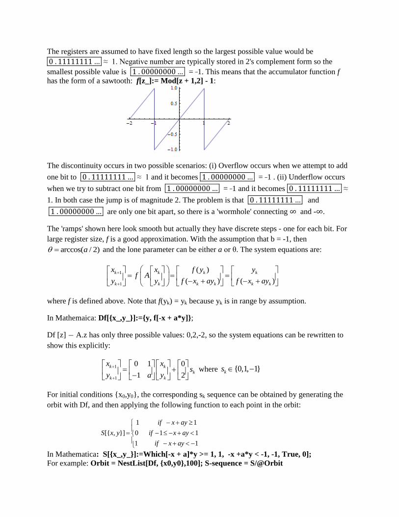
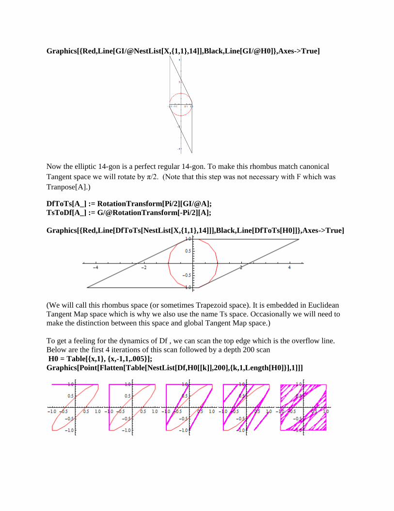