Effective Hamiltonians and Averaging for Hamiltonian ...

Arch. Rational Mech. Anal. 157 (2001) 1–33Digital Object Identifier (DOI) 10.1007/s002050100128

Effective Hamiltonians and Averaging forHamiltonian Dynamics I

L. C. Evans & D. Gomes

Communicated by the Editors

Abstract

This paper, building upon ideas of Mather, Moser, Fathi, E and others, appliesPDE (partial differential equation) methods to understand the structure of certainHamiltonian flows. The main point is that the “cell” or “corrector” PDE, intro-duced and solved in a weak sense by Lions, Papanicolaou and Varadhan in theirstudy of periodic homogenization for Hamilton-Jacobi equations, formally inducesa canonical change of variables, in terms of which the dynamics are trivial. Weinvestigate to what extent this observation can be made rigorous in the case that theHamiltonian is strictly convex in the momenta, given that the relevant PDE doesnot usually in fact admit a smooth solution.

1. Introduction

This is the first of a projected series of papers that develop PDE techniques tounderstand certain aspects of Hamiltonian dynamics with many degrees of freedom.

1.1. Changing variables

The basic issue is this. Given a smooth HamiltonianH : Rn × R

n → R,H = H(p, x), we wish to examine the Hamiltonian flow

x = DpH(p, x),

p = −DxH(p, x)(1.1)

under a canonical change of variables

(p, x) → (P,X), (1.2)

2 L. C. Evans & D. Gomes

wherep = Dxu(P, x),

X = DPu(P, x)(1.3)

for a generating functionu : Rn × R

n → R, u = u(P, x). Here we writeDx =( ∂∂x1

), . . . , ∂∂xn

) andDP = ( ∂∂P1

. . . , ∂∂Pn

). Assuming that we can find a smoothfunctionu to solve the Hamilton-Jacobi type PDE

H(Dxu(P, x), x) = H (P ) in Rn, (1.4)

and supposing as well that we can invert the relationships(1.3) to solve forP,X

as smooth functions ofp, x, a calculation shows that we thereby transform(1.1)into the trivial dynamics

X = DH(P),

P = 0.(1.5)

In terms of mechanics,P is an “action” andX an “angle” or “rotation” variable, asfor instance inGoldstein [Gd].

Of course we cannot really carry out this classical procedure in general, sincethe PDE(1.4) does not usually admit a smooth solution and, even if it does, thetransformation(1.2), (1.3) is not usually globally defined. Only very special Hamil-tonians are integrable in this sense.

1.2. Homogenization

On the other hand, under some reasonable hypotheses we can in fact buildappropriateweak solutions of(1.4), as demonstrated within another context in theclassic-but-unpublished paper byLions, Papanicolaou & Varadhan [L-P-V].These authors look at the initial value problem for the Hamilton-Jacobi PDE

uεt + H(Dxu

ε,x

ε

)= 0 in R

n × (0,∞),

uε = g onRn × {t = 0},

(1.6)

under the primary assumption that the mappingx �→ H(p, x) is Tn-periodic,

whereTn denotes the flat torus, that is, the unit cube inR

n, with opposite facesidentified. Consequently asε → 0, the nonlinearity in(1.6) is rapidly oscillating;and the problem is to understand the limiting behavior of the solutionsuε. Lionsetal. show under some mild additional hypotheses on the Hamiltonian thatuε → u,the limit functionu solving a Hamilton-Jacobi PDE of the form

ut + H (Dxu) = 0 in Rn × (0,∞),

u = g onRn × {t = 0}. (1.7)

HereH : Rn → R, H = H (P ), is theeffective (or averaged) Hamiltonian,

and is built fromH as follows.

Effective Hamiltonians and Averaging for Hamiltonian Dynamics I 3

1.3. How to construct H

First, consider for fixedP ∈ Rn thecell (or corrector) problem

H(P + Dxv, x) = λ in Rn,

x �→ v is Tn-periodic.

As proved inLions, Papanicolaou & Varadhan [L-P-V] (and recounted in [E2]and inBraides & Defranceschi [B-D, Sect. 16.2]), there exists a unique realnumberλ for which there exists a viscosity solution. We may thendefine

H (P ) := λ,

and so rewrite the foregoing as

H(P + Dxv, x) = H (P ) in Rn,

x �→ v is Tn-periodic.

(1.8)

Once we setu(P, x) := P · x + v(P, x), (1.9)

the PDE in(1.8) is just(1.4).

Remark. We pause here to draw attention to some simple observations relatingthe cell problem(1.8) and semiclassical approximations in quantum mechanics forperiodic potentials. These comments are intended as further motivation.

Consider the time-independent Schr¨odinger equation

− h2

2�ψ + Vψ = Eψ in R

n, (1.10)

whereh is Planck’s constant,V : Rn → R is a T

n-periodic potential, andE isthe energy corresponding to the eigenstateψ : R

n → C. A standard textbookprocedure is to look for a solution having theBloch wave form

ψ = ei P ·x

h φ, (1.11)

whereφ : Rn → C isT

n-periodic. We further supposeφ to have the WKB structure

φ = aeivh (1.12)

for periodica, v : Rn → R. Substituting(1.11), (1.12) into (1.10) and taking real

parts yields12|P + Dxv|2 + V (x) = E, (1.13)

up to terms formally of sizeO(h).Thus in the semiclassical limith → 0, we heuristically obtain the cell problem

(1.8) for the HamiltonianH(p, x) = 12|p|2 + V (x) andH (P ) = E.


1.4. Questions, absolute minimizers

The procedure outlined in Subsection 1.3 provides us with at least a theoreticalconstruction ofH and of a generating functionu. Returning then to the commentsin Subsection 1.1, we can now formulate these

Basic Questions. To what extent can we employ H and u to understand thesolutions of the Hamiltonian flow (1.1)? In particular, how is information aboutthe dynamics “encoded” into H?

These are really hard issues, and to make at least a little progress we will needsome additional hypotheses on both the Hamiltonian and the particular trajectoriesof the ODE (ordinary differential equation) we examine. Let us henceforth supposethat the mappingp �→ H(p, x) is uniformly convex, in which case we can associatewith H theLagrangian

L(q, x) := maxp

(p · q − H(p, x)).

Consider then a Lipschitz curvex(·)which minimizes the associated action integral,meaning that ∫ T

0L(x, x) dt �

∫ T

0L(y, y) dt (1.14)

for each timeT > 0 and each Lipschitz curvey(·) with x(0) = y(0), x(T ) = y(T ).We callx(·) a (one-sided)absolute minimizer. If we as usual define themomentum

p := DqL(x, x),

then(x(·),p(·)) satisfy Hamilton’s ODE(1.1).A discovery ofAubry [A], Mather [Mt1,Mt2,Mt3,Mt4], Fathi [F1,F2,F3],

Moser [Ms], E [EW2], etc., is that solutions of(1.1) corresponding to absoluteminimizers are somehow “better” than other solutions. Indeed, these authors haveshown that the Hamiltonian dynamics are in some sense “integrable” for suchspecial trajectories. The main goal of our work is to continue this analysis, withparticular emphasis upon PDE methods (based upon viscosity solutions of(1.8)),applied to problems with many degrees of freedom.

1.5. Outline

In Section 2 below we review the definition of the effective HamiltonianH ,introduce the corresponding effective LagrangianL, and recall the connectionswith the large-time asymptotics of absolute minimizersx(·).

We then rescale in timex(·) andp(·) in Section 3, and introduce certain Youngmeasures{νt }t�0 on phase space, which record the oscillations of the rescaled func-tions in asymptotic limits. These measures contain information about the Hamil-tonian flow, and so our goal in subsequent sections is understanding their struc-ture. In§4 we show that eachν = νt is supported on the graph of the mappingp = Dxu(P, x) and furthermore “stays away” from the discontinuities inDxu.


In Section 5 we prove thatu is well behaved on the support ofσ , the projectionof ν ontox-space. For this, we firstly derive the formalL2 bound∫

Tn

|D2xu|2dσ � C (1.15)

and then theL∞ estimate|D2

xu| � C σ -a.e. (1.16)

We rigorously establish some analogues of(1.15), (1.16), entailing difference quo-tients in thex-variables. As an application, we provide in Section 6 a newproofof Mather’s theorem thatν is supported on ann-dimensional Lipschitz continuousgraph.

Section 7 extends the techniques from Section 5 to establish what amounts toanL2 estimate for the mixed second partial derivatives,∫

Tn

|D2xP u|2dσ � CD2H (P ). (1.17)

More precisely, we prove a similar inequality involving difference quotients in thevariableP .An application of this bound appears in Section 8, where we demonstratethe strict convexity ofH in certain directions.

In Section 9 we draw some further deductions under the assumptions thatH isdifferentiable atP and the components ofQ := DH(P )are rationally independent.

A forthcoming companion paper [E-G2] addresses problems with time-depend-ent Hamiltonians. The primary new topics developed there include a weak inter-pretation of the “adiabatic invariance of the action” and a discussion of the Berry-Hannay geometric phase correction, computed in terms of effective Hamiltonians.

Our work is strongly related to some extremely interesting papers ofFathi [F1,F2,F3], which develop his “weak KAM (Kolmogorov-Arnol’d-Moser) theory”. Wehope later to work out more clearly some of the connections with Fathi’s discoveries.

Some other relevant papers includeMather [Mt1,Mt2,Mt3,Mt4],Weinan E[EW1,EW2],Gomes [G], Sobolevskii [So1,So2],Mane [Mn2,Mn3], Jauslin,Kreiss & Moser [J-K-M], Iturriaga [I], Dias Carneiro [DC], Arisawa [Ar],etc. A good survey isMather & Forni [M-F], and we have foundMane’s book[Mn1] to be very useful.

SeeConcordel [C1,C2],Chou & Duffin [C-D], Nussbaum [N], etc. forconnections with nonlinear additive eigenvalue problems.Fathi [F4], Namah &Roquejoffre [N-F], Roquejoffre [R], Barles & Souganidis [B-S] andFathi& Mather [F-M] discuss some related questions about large-time asymptotics ofsolutions to Hamilton-Jacobi equations. Similar problems for stochastic homoge-nization have been studied byRezakhanlou [Rz] andSouganidis [S].

There is also a large literature for time-dependent Hamiltonians with one degreeof freedom. In this setting ordering properties for minimizing trajectories providepowerful tools unavailable in higher dimensions. SeeMather & Forni [M-F],Aubry [A], Bangert [B2], etc. for more.


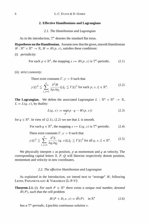
2. Effective Hamiltonians and Lagrangians

2.1. The Hamiltonian and Lagrangian

As in the introduction,Tn denotes the standard flat torus.

Hypotheses on the Hamiltonian. Assume now that the given, smooth HamiltonianH : R

n × Rn → R, H = H(p, x), satisfies these conditions:

(i) periodicity:

For eachp ∈ Rn, the mappingx �→ H(p, x) is T

n-periodic. (2.1)

(ii) strict convexity:

There exist constants&, γ > 0 such that

γ |ξ |2 �n∑

i,j=1

∂2H

∂pi∂pjξiξj � &|ξ |2 for eachp, x, ξ ∈ R

n.(2.2)

The Lagrangian. We define the associatedLagrangian L : Rn × R

n → R,L = L(q, x), by duality:

L(q, x) := supp(p · q − H(p, x)) (2.3)

for q ∈ Rn. In view of (2.1), (2.2) we see thatL is smooth.

For eachq ∈ Rn, the mappingx �→ L(q, x) is T

n-periodic. (2.4)

There exist constants&, γ > 0 such that

γ |ξ |2 �n∑

i,j=1

∂2L

∂qi∂qj(q, x)ξiξj � &|ξ |2 for all q, x, ξ ∈ R

n. (2.5)

We physically interpretx as position,p as momentum andq as velocity. Thecorresponding capital lettersX,P,Q will likewise respectively denote position,momentum and velocity in new coordinates.

2.2. The effective Hamiltonian and Lagrangian

As explained in the Introduction, we intend next to “average”H , followingLions, Papanicolaou & Varadhan [L-P-V]:

Theorem 2.1. (i) For each P ∈ Rn there exists a unique real number, denoted

H (P ), such that the cell problem

H(P + Dxv, x) = H (P ) in Rn (2.6)

has a Tn-periodic, Lipschitz continuous solution v.


(ii) In addition, there exists a constant α such that

D2xv � αI in R

n (2.7)

in the distribution sense.

We call the functionH : R

n → R (2.8)

so defined theeffective or averaged Hamiltonian.

Remarks. (i) We understandv to solve(2.6) in the sense of viscosity solutions.This means that ifφ = φ(x) is a smooth function and

v − φ has a maximum (minimum) at a pointx0 ∈ Rn, then

H(P + Dφ(x0), x0) � H (P ) (� H (P )).(2.9)

We will in fact mostly need only thatv is differentiable a.e. with respect ton-dimensional Lebesgue measure, and thatv solves the PDE(2.6) at any pointof differentiability.

(ii) The inequality(2.7) means that

the functionv(x) := v(x) − α

2|x|2 is concave onRn. (2.10)

(iii) If v is a solution of(2.6), we will hereafter often write

v = v(P, x) (P, x ∈ Rn)

to emphasize the dependence onP .

GivenH as above, we define also theeffective Lagrangian

L(Q) := supP

(P · Q − H (P )) (2.11)

for Q ∈ Rn.

2.3. Properties of H and L

Proposition 2.2. The mappings

P �→ H (P ), Q �→ L(Q)

are convex and real-valued. Furthermore, H and L are superlinear:

lim|P |→∞H (P )

|P | = lim|Q|→∞L(Q)

|Q| = +∞. (2.12)


Proof. (1) SeeLions, Papanicolaou & Varadhan [L-P-V] (or [E2]) for a proofthatH is convex. The convexity ofL is immediate from(2.11).

(2) In view of (2.2),

H (P ) � α|P + Dxv|2 − β � α|P |2 + 2αP · Dxv − β a.e. (2.13)

for appropriate constantsα > 0, β � 0. We integrate this inequality overTn and

recallv is periodic, to deduce

H (P ) � α|P |2 − β.

ThusH is superlinear, and in particularL(Q) < ∞ for eachQ. On the other hand,by constructionH (P ) < ∞ for eachP ; whence the duality formula

H (P ) = supQ

(P · Q − L(Q))

impliesL is superlinear. ��In later sections we will relateH, L to appropriately rescaled minimizers of the

action functionals, and for this will several times invoke the following results ofLions, Papanicolaou & Varadhan [L-P-V, §IV]. (See alsoWeinan E [EW1],Braides & Defranceschi [B-D, § 16.2].)

Theorem 2.3. (i) If X : [0, T ] → Rn is a Lipschitz continuous curve and xε(·) →

X(·) uniformly, then

∫ T

0L(X) dt � lim inf

∫ T

0L

(xε,

xεε

)dt. (2.14)

(ii) Define

Sε(x, y, t) := inf

{∫ t

0L

(x,

xε

)ds | x(t) = x, x(0) = y

}(2.15)

for x, y ∈ Rn, t > 0. Then

Sε(x, y, t) → tL

(x − y

t

)as ε → 0, (2.16)

uniformly on compact subsets of Rn × R

n × (0,∞).

3. Young measures

Next we study the asymptotic behavior ast → ∞ of certain curves that mini-mize the action.


3.1. Hamilton’s ODE, rescalings

Definition. A Lipschitz continuous curvex : [0,∞) → Rn is called a (one-sided)

absolute minimizer if

∫ T

0L(x, x) dt �

∫ T

0L(y, y) dt (3.1)

for each timeT > 0 and each Lipschitz continuous curvey : [0,∞) → Rn such

that

x(0) = y(0), x(T ) = y(T ).

Given as above an absolutely minimizing curvex(·), define the correspondingmomentum

p(t) := DqL(x(t), x(t)) (3.2)

for t � 0. Then

x(t) = DpH(p(t), x(t)),

p(t) = −DxH(p(t), x(t))(3.3)

for t � 0.We wish to understand the pair(x(·),p(·)) for large times, and to this end

introduce therescaled dynamics

xε(t) := εx(t/ε), pε(t) := p(t/ε),

xε(0) = εx(0), pε(0) = p(0).

It follows from (3.3) that

xε(t) = DpH

(pε(t),

xε(t)ε

),

pε(t) = −1

εDxH

(pε(t),

xε(t)ε

) (3.4)

for t � 0.

Remark. Since ddtH

(pε(t),

xε(t)ε

)= 0, we have supt�0 H

(pε(t),

xε(t)ε

)� C for

some constantC, independent ofε. ButH(p, x) � γ2 |p|2 − C, and so

supt�0

{|pε(t)|, |xε(t)|} < ∞. (3.5)


3.2. Recording oscillations

We expect the functionspε(·) and xε(·)ε

(modTn) to oscillate asε → 0, and so

introduce measures on phase space to record these motions. Invoking for instancethe methods from§1.E of [E1], we have

Proposition 3.1. There exists a sequence εk → 0 and for a.e. t > 0 a Radonprobability measure νt on R

n × Tn such that

3

(pεk (t),

xεk (t)εk

)⇀ 3(t) :=

∫Rn

∫Tn

3(p, x) dνt (p, x) (3.6)

for each bounded, continuous function

3 : Rn × R

n → R, 3 = 3(p, x),

such that x �→ 3(p, x) is Tn-periodic.

We call{νt }t�0 Young measures associated with the dynamics(3.4).

Remark. The limit (3.6) means∫ T

03

(pεk ,

xεkεk

)ζ dt →

∫ T

03ζ dt (3.7)

for eachT > 0 and each smooth functionζ : [0, T ] → R.

Lemma 3.2. The support of the measure νt is bounded, uniformly in t .

This is clear from(3.5).

Lemma 3.3. For each C1 function 3 as above,∫Rn

∫Tn

{H,3} dνt = 0 (3.8)

for a.e. t � 0, where

{H,3} := DpH · Dx3 − DxH · Dp3 (3.9)

is the Poisson bracket.

The identity(3.8) means that the measureνt is invariant under the Hamiltonianflow (3.3).

Proof. We haved

dt3

(pε,

xεε

)= Dp3 · pε + Dx3 · xε

ε

= 1

ε{H,3}

according to(3.4). Takeζ : [0, T ] → R to be smooth, with compact support. Then∫ T

0{H,3}

(pε,

xεε

)ζ dt = −

∫ T

0εζ3

(pε,

xεε

)dt.

Sendingε = εk → 0, we deduce(3.8). ��


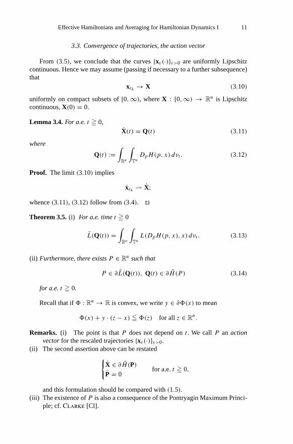
3.3. Convergence of trajectories, the action vector

From (3.5), we conclude that the curves{xε(·)}ε>0 are uniformly Lipschitzcontinuous. Hence we may assume (passing if necessary to a further subsequence)that

xεk → X (3.10)

uniformly on compact subsets of[0,∞), whereX : [0,∞) → Rn is Lipschitz

continuous,X(0) = 0.

Lemma 3.4. For a.e. t � 0,

X(t) = Q(t) (3.11)

where

Q(t) :=∫

Rn

∫Tn

DpH(p, x) dνt . (3.12)

Proof. The limit (3.10) implies

xεk ⇀ X;whence(3.11), (3.12) follow from (3.4). ��Theorem 3.5. (i) For a.e. time t � 0

L(Q(t)) =∫

Rn

∫Tn

L(DpH(p, x), x) dνt . (3.13)

(ii) Furthermore, there exists P ∈ Rn such that

P ∈ ∂L(Q(t)), Q(t) ∈ ∂H (P ) (3.14)

for a.e. t � 0.

Recall that if3 : Rn → R is convex, we writey ∈ ∂3(x) to mean

3(x) + y · (z − x) � 3(z) for all z ∈ Rn.

Remarks. (i) The point is thatP does not depend ont . We callP an actionvector for the rescaled trajectories{xε(·)}ε>0.

(ii) The second assertion above can be restated{X ∈ ∂H (P)P = 0

for a.e.t � 0,

and this formulation should be compared with(1.5).(iii) The existence ofP is also a consequence of the Pontryagin Maximum Princi-

ple; cf.Clarke [Cl].


Proof. (1) Letyε := xε(0) = εx(0) → 0. According to Theorem 2.3,

Sεk (x, yεk , t) → tL(xt

)(x ∈ R

n, t > 0), (3.15)

uniformly on compact subsets. But

Sε(x, yε, t) = inf

{∫ t

0L

(x,

xε

)ds | x(t) = x, x(0) = yε

},

and so

Sε(xε(t), yε, t) =∫ t

0L

(xε,

xεε

)ds, (3.16)

since the curvexε(·) is an absolute minimizer.(2) From(3.10), (3.15) we see that

Sεk (xεk (t), yεk , t) → tL

(X(t)

t

). (3.17)

But then(3.16) implies that

L

(xεk ,

xεkεk

)⇀

d

dt

(tL

(Xt

)). (3.18)

Now

d

dt

(tL

(Xt

))∈ L

(Xt

)+ ∂L

(Xt

) (X − X

t

)� L(X), (3.19)

by convexity. Consequently, sincexε = DpH(pε,

xεε

), we deduce from(3.18) that∫

Rn

∫Tn

L(DpH(p, x), x) dνt � L(X(t)) (3.20)

for a.e.t > 0.Conversely, Theorem 2.3 implies

∫ b

a

L(X(t)) dt � limε→0

∫ b

a

L(

xε,xεε

)dt =

∫ b

a

∫Rn

∫Tn

L(DpH, x) dνt dt

for all 0 � a < b < ∞ and so

L(X(t)) �∫

Rn

∫Tn

L(DpH(p, x), x) dνt

for a.e.t . This and(3.20) establish(3.13).(3) In particular,

d

dt

(tL

(X(t)

t

))= L(X(t)) = L(Q(t)) a.e.;


and so1

T

∫ T

0L(Q(t)) dt = 1

T

∫ T

0

d

dt

(tL

(X(t)

t

))dt

= L

(X(T )

T

)

= L

(1

T

∫ T

0Q(t) dt

).

(3.21)

This identity, valid for each timeT > 0, implies that{Q(t)}t�0 lies in a supportingdomain ofL. This means that

P ∈ ∂L(Q(t)) for a.e. timet � 0 (3.22)

for some vectorP ∈ Rn. Equivalently,Q(t) ∈ ∂H (P ).

To confirm(3.22), fix a timeT > 0, write Q := 1T

∫ T

0 Q(t) dt , and take anyP ∈ ∂L(Q). Then owing to(3.21) we have

L(Q(t)) = L(Q) + P · (Q(t) − Q)

for a.e. time 0� t � T . ThusQ(t) is a minimizer of the convex functionL(Q) −L(Q) − P · (Q − Q), and soP ∈ ∂L(Q(t)), for a.e. time 0� t � T . Taking asequence of timesTk → ∞ and passing if necessary to a subsequence, we obtaina vectorP satisfying(3.22). ��

4. Structure of minimizing measures

We next fix one of the Young measuresνt and hereafter writeν = νt . Our goalis to understand the form of this measure, and in particular to describe its support.

Our further deductions will be based entirely upon certain conclusions reachedabove. These are firstly thatν is a compactly supported Radon probability measureonR

n × Tn, for which we define

Q :=∫

Rn

∫Tn

DpH(p, x) dν,

as in(3.12) above. In addition, we have∫Rn

∫Tn

{H,3} dν = 0 (4.1)

for eachC1 function3 that isTn-periodic in the variablex, and furthermore

L(Q) =∫

Rn

∫Tn

L(DpH(p, x), x) dν. (4.2)

These are, respectively, assertions(3.8) and(3.13) above.

Remarks. Our ν is therefore aminimal measure in the sense ofMather [Mt1],except that we work in phase space. The advantage is that the flow invariancecondition(4.1) is fairly simple, and very useful, in the(p, x) variables.


Notation. (i) We writeM := spt(ν) and callM theAubry-Mather set.(ii) We denote byσ theprojection of ν onto thex-variables. That is,

σ(E) := ν(Rn × E)

for each Borel subsetE of Tn.

Take now anyP ∈ ∂L(Q) and letv = v(P, x) be any viscosity solution of thecorresponding cell problem

H(P + Dxv, x) = H (P ) in Rn,

x �→ v(P, x) is Tn-periodic,

(4.3)

satisfying the semiconcavity condition(2.7). We hereafter set

u(P, x) := P · x + v(P, x).

4.1. Differentiability on the support of ν

Theorem 4.1. (i) The function u is differentiable in the variable x σ -a.e., andσ -a.e. point is a Lebesgue point for Dxu.

(ii) This equality holds:

p = Dxu(P, x) ν-a.e.

(iii) Furthermore,

∫Rn

∫Tn

H(p, x) dν =∫

Tn

H(Dxu, x) dσ = H (P ); (4.4)

and if H is differentiable at P ,

∫Rn

∫Tn

DpH(p, x) dν =∫

Tn

DpH(Dxu, x) dσ = DH(P ).

In particular, the PDE(4.3) holds pointwise,σ -a.e.

Remarks. Formula(4.4) explicitly displaysH as an average ofH ; but for this tobe useful, we need to know more about the measureσ . We will later, in Section 9,discover a bit more about the structure ofσ .

Observe also that from(4.4) we deduce

H (P ) = H (P ) if P, P ∈ ∂L(Q). (4.5)

Finally, compare assertion (ii) with the canonical change of variables(1.3).


Proof. (1) To ease notation, we do not display the dependence ofu on the variableP , and we writeDu for Dxu.

Takeηε to be a smooth, nonnegative, radial convolution kernel, supported inthe ballB(0, ε). Then set

uε := ηε ∗ u.

The strict convexity ofH implies for allp, q ∈ Rn that

H(q, x) � H(p, x) + DpH(p, x) · (q − p) + γ

2|q − p|2.

Takeq = Du(y), p = Duε(x) = ∫Rn ηε(x − y)Du(y) dy in this expression,

multiply by ηε(x − y), and then integrate with respect toy:

H(Duε(x), x) �∫

Rn

ηε(x − y)H(Du(y), x) dy

− γ

2

∫Rn

ηε(x − y)|Du(y) − Duε(x)|2dy.

Since the PDEH(Dxu, x) = H (P ) holds pointwise a.e., we conclude that

βε(x) + H(Duε(x), x) � H (P ) + Cε (4.6)

for eachx ∈ Tn, where

βε(x) := γ

2

∫Rn

ηε(x − y)|Du(y) − Duε(x)|2 dy. (4.7)

(2) Recalling again the strict convexity ofH with respect to the variablep, wededuce

γ

2

∫Rn

∫Tn

|Duε(x) − p|2 dν

�∫

Rn

∫Tn

H(Duε(x), x) − H(p, x) − DpH(p, x) · (Duε(x) − p) dν.

(4.8)NowDuε = P + Dvε, wherevε = ηε ∗ v is periodic. Consequently∫

Rn

∫Tn

DpH · Dvε dν = 0,

according to(4.1). This observation and(4.6) imply

γ

2

∫Rn

∫Tn

|Duε − p|2 dν +∫

Tn

βε dσ

� H (P ) −∫

Rn

∫Tn

H + DpH · (P − p) dν + Cε.

(4.9)Next,P ∈ ∂L(Q) implies

L(Q) + H (P ) = P · Q.


Furthermore

L(DpH(p, x), x) + H(p, x) = DpH(p, x) · p.Recalling thatQ = ∫

Rn

∫Tn DpH dν and substituting this into(4.9), we find

γ

2

∫Rn

∫Tn

|Duε − p|2 dν +∫

Tn

βε dσ

� −L(Q) +∫

Rn

∫Tn

L(DpH, x) dν + Cε

= Cε,

(4.10)

according to(4.2).(3) Now sendε → 0. Passing as necessary to a subsequence we deduce first

from (4.10) thatβε → 0 σ -a.e.

Thusσ -a.e. pointx is a point of approximate continuity ofDu, andDu is σ -measurable. Sinceu = x ·P + v andv is semiconcave as a function ofx (Theorem2.1 (ii)), it follows thatu is differentiable inx, σ -a.e. Thus

Duε → Du

pointwise,σ -a.e., and so(4.10) in turn forces

p = Du(x) = P + Dv(x) ν-a.e.

This proves assertion (ii), and (iii) follows then from the cell PDE.��Remark. As a consequence of the foregoing proof, we have the identity∫

Rn

∫Tn

DpH(p, x) · Dxv dν =∫

Tn

DpH(Dxu, x) · Dxv dσ = 0, (4.11)

which we will need later. To confirm this, recall from above that∫Rn

∫Tn

DpH · Dxvε dν = 0.

SinceDxvε → Dxv boundedly,ν-a.e., we can apply the Dominated Convergence

Theorem.

5. Derivative estimates in the variable x

We devote this section to showing that our solutionu of the cell problem is“smoother” on the support ofσ than it may be at other points ofT

n. This is a sortof “partial regularity” assertion.


5.1. Formal L2 and L∞ estimates

First of all, we provide for the reader some purely formalL2 andL∞ estimatesforD2

xu on the support ofσ , calculations which provide motivation for the rigorousbounds obtained afterwards.

L2 inequalities. We assume for this that the generating functionu is smooth, thendifferentiate the cell PDE twice with respect toxi , and finally sum fori = 1, . . . , n:

Hpkpl (Dxu, x)uxkxi uxlxi + Hpk (Dxu, x)uxkxixi

+ 2Hpkxi (Dxu, x)uxkxi + Hxixi (Dxu, x) = 0.

The first term on the left-hand side is greater than or equal toγ |D2xu|2. Thus

γ

∫Tn

|D2xu|2 dσ +

∫Tn

DpH · Dx(�xu) dσ � C + C

∫Tn

|D2xu| dσ.

Since�xu = �xv is periodic, the second term on the left-hand side equals zero,according to(4.1). We consequently conclude that∫

Tn

|D2xu|2 dσ � C, (5.1)

for some constantC depending only onH andP . ��L∞ inequalities. We can similarly differentiate the cell PDE twice in any unitdirectionξ , to find

Hpkpl (Dxu, x)uxkξuxlξ + Hpk (Dxu, x)uxkξξ

+ 2Hpkξ (Dxu, x)uxkξ + Hξξ (Dxu, x) = 0,

for uξξ := ∑ni,j=1 uxixj ξiξj . Take a nondecreasing, function3 : R → R, and write

φ := 3′ � 0. Multiply the above identity byφ(uξξ ), and integrate with respect toσ . After some simplifications, we find

γ

2

∫Tn

|Dxuξ |2φ(uξξ ) dσ +∫

Tn

DpH · Dx(3(uξξ )) dσ � C

∫Tn

φ(uξξ ) dσ.

Sinceuξξ = vξξ is periodic, the second term on the left-hand side is zero. We select

φ(z) ={

1 if z � −µ

0 if z > −µ,

for a constantµ > 0. Since|Dxuξ |2 � u2ξξ , we conclude thatσ({uξξ � −µ}) = 0

if µ is large enough. Because(2.10) provides the opposite estimateuξξ � α, wethereby derive the formal bound

|uξξ | � C σ -a.e., (5.2)

the constantC depending only upon known quantities.��


Remark. As the interested reader may wish to confirm, the foregoing derivationsare especially transparent for the classical Hamiltonian

H(p, x) = 12|p|2 + V (x),

in which case the cell PDE(4.3) is theeikonal equation

12|Dxu|2 + V (x) = H (P )

and(4.1) corresponds to thetransport equation

div(σDxu) = 0.

A clear message is that these two PDE should be considered together as a pair, inaccordance with formal semiclassical limits. (See the Remark in Subsection 1.3.)

5.2. An L2-estimate of difference quotients in x

We now establish an analogue of estimate(5.1), with difference quotients re-placing some of the derivatives.

Theorem 5.1. There exists a constant C, depending only on H and P , such that∫Tn

|Dxu(P, x + h) − Dxu(P, x)|2 dσ � C|h|2 (5.3)

for h ∈ Rn.

Remark. If Dxu(P, x + h) is multivalued, we interpret(5.3) to mean∫Tn

|ξ − Dxu|2 dσ � C|h|2 (5.4)

for someσ -measurable selectionξ ∈ Dxu(P, · + h).

Proof. (1) To simplify notation we do not display the dependence ofu onP , andjust writeDu for Dxu.

Fix h ∈ Rn and define the shifted function

u(·) := u(· + h).

ThenH(Du, x + h) = H (P ) a.e. inR

n.

Mollifying as in the proof of Theorem 4.1, we have

H(Duε, x + h) � H (P ) + Cε in Rn.

Therefore

H(Duε, x) − H(Du, x) � Cε + H(Duε, x) − H(Duε, x + h)


σ -a.e., and consequently

γ

2

∫Tn

|Duε − Du|2 dσ +∫

Tn

DpH(Du, x) · (Duε − Du) dσ

� Cε +∫

Tn

H(Duε, x) − H(Duε, x + h) dσ

� C(ε + |h|2) −∫

Tn

DxH(Duε, x) · h dσ.

(5.5)

(2) SinceDuε − Du = Dvε − Dv, the second term on the left-hand side of(5.5) vanishes, in view of(4.1), (4.11). Therefore

γ

2

∫Tn

|Duε − Du|2 dσ � C(ε + |h|2) −∫

Tn

DxH(Du, x) · h dσ

+ C

∫Tn

|Duε − Du||h| dσ,and thus

γ

4

∫Tn

|Duε − Du|2 dσ � C(ε + |h|2) −∫

Rn

∫Tn

DxH · h dν.However(4.1) implies the last term here is zero; whence∫

Tn

|Duε − Du|2 dσ � C(ε + |h|2). (5.6)

(3) We sendε → 0. Passing as necessary to a subsequence we have

Duε ⇀ ξ weakly inL2σ

and ∫Tn

|ξ − Du|2 dσ � C|h|2. (5.7)

(4) To conclude, we must show

ξ ∈ Du = Du(· + h) σ -a.e., (5.8)

which means that forσ -a.e. pointx there exists a constantC such that

u(y) � u(x) + ξ · (y − x) + C|y − x|2 (5.9)

for all y. To confirm this, recall thatu, and so alsouε, are semiconcave:

uε(y) � uε(x) + Duε(x) · (y − x) + C|y − x|2for all x, y. Takeg ∈ L2

σ , g � 0. Then fixingy and integrating the variablex withrespect toσ , we find

0 �∫

Tn

(−uε(y) + uε(x) + Duε(x) · (y − x) + C|y − x|2)g(x) dσ(x).Let ε → 0 and noteuε → u uniformly. We conclude that

0 �∫

Tn

(−u(y) + u(y) + ξ · (y − x) + C|y − x|2)g(x) dσ(x).This inequality is true for allg as above; whence(5.7) holds forσ -a.e. pointx andall y. ��


5.3. L∞ estimates of difference quotients in x

We next refine the integration arguments above, to derive anL∞ bound onsecond-order difference quotients. This will be a variant of the formal estimate(5.2) above.

Theorem 5.2. There exists a constant C, depending only on H and P , such that

|u(P, x + h) − 2u(P, x) + u(P, x − h)| � C|h|2 (5.10)

for all h ∈ Rn and each point x ∈ spt(σ ).

Proof. (1) Takeh �= 0, and write

u = u(· + h), u = u(· − h).

We consider, as before, the mollified functionsuε, uε, where we take

0 < ε � η|h|2 (5.11)

for smallη > 0. As in the earlier proofs, we have

H(Duε, x + h) � H (P ) + Cε,

H(Duε, x − h) � H (P ) + Cε.

Therefore forσ -a.e. pointx,

H(Duε, x) − 2H(Du, x) + H(Duε, x)

� Cε + H(Duε, x) − H(Duε, x + h)

+ H(Duε, x) − H(Duε, x − h).

Henceγ

2(|Duε − Du|2 + |Duε − Du|2) + DpH(Du, x) · (Duε − 2Du + Duε)

� C(ε + |h|2) + (DxH(Duε, x) − DxH(Duε, x)) · h,and consequently

γ

4(|Duε − Du|2 + |Duε − Du|2)

+ DpH(Du, x) · (Duε − 2Du + Duε) � C(ε + |h|2).(2) Fix now a smooth, nondecreasing, function3 : R → R, and writeφ :=

3′ � 0. Multiply the last inequality above byφ(uε−2u+uε

|h|2), and integrate with

respect toσ :

γ

4

∫Tn

(|Duε − Du|2 + |Duε − Du|2)φ(uε − 2u + uε

|h|2)

dσ

+∫

Tn

DpH(Du, x) · (Duε − 2Du + Duε)φ(· · · ) dσ

� C(ε + |h|2)∫

Tn

φ(· · · ) dσ.

(5.12)


Now the second term on the left-hand side of(5.12) equals

|h|2∫

Rn

∫Tn

DpH(p, x) · Dx3

(uε − 2u + uε

|h|2)

dν (5.13)

and thus is zero. (To see this, note from(4.1) that the expression(5.13) vanishes ifwe replaceu by a mollified functionuδ. Let δ → 0, recalling the estimates in theproof of Theorem 4.1.)

So now dropping the above term from(5.12) and rewriting, we deduce∫Tn

|Duε(x + h) − Duε(x − h)|2φ(uε(x + h) − 2u(x) + uε(x − h)

|h|2)

dσ

� C(ε + |h|2)∫

Tn

φ

(uε(x + h) − 2u(x) + uε(x − h)

|h|2)

dσ.

(5.14)(3) We confront now a technical problem, as(5.14) entails a mixture of first-

order difference quotients forDuε and second-order difference quotients foru, uε.We can however relate these expressions, sinceu is semiconcave.

To see this, first of all define

Eε := {x ∈ spt(σ ) | uε(x + h) − 2u(x) + uε(x − h) � −µ|h|2}, (5.15)

the large constantµ > 0 to be fixed below. Now according to(2.10), the functions

u(x) := u(x) − α

2|x|2, uε(x) := uε(x) − α

2|x|2 (5.16)

are concave. Also a pointx ∈ spt(σ ) belongs toEε if and only if

uε(x + h) − 2u(x) + uε(x − h) � −(µ + α)|h|2. (5.17)

Set

f ε(s) := uε(x + s

h

|h|)

(−|h| � s � |h|). (5.18)

Thenf is concave, and

uε(x + h) − 2uε(x) + uε(x − h) = f ε(|h|) − 2f ε(0) + f ε(−|h|)

=∫ |h|

−|h|f ε′′

(x)(|h| − |s|) ds

� |h|∫ |h|

−|h|f ε′′

(s) ds (sincef ε′′ � 0)

= |h|(f ε′(|h|) − f ε′

(−|h|))= (Duε(x + h) − Duε(x − h)) · h.

Consequently ifx ∈ Eε, this inequality and(5.17) together imply

2|uε(x) − u(x)| + |Duε(x + h) − Duε(x − h)||h| � (µ + α)|h|2.


Now |uε(x)−u(x)| � Cε onTn, sinceu is Lipschitz continuous. We may therefore

takeη in (5.11) small enough to deduce from the foregoing that

|Duε(x + h) − Duε(x − h)| �(µ

2+ α

)|h|. (5.19)

But then

|Duε(x + h) − Duε(x − h)| �(µ

2− α

)|h|. (5.20)

(4) Return now to(5.14). Takingµ > 2α and

φ(z) ={

1 if z � −µ,

0 if z > −µ,

we discover from(5.14) that

(µ2

− α)2|h|2σ(Eε) � C(ε + |h|2)σ (Eε).

We fixµ so large that (µ2

− α)2

� C + 1,

to deduce

(|h|2 − Cε)σ(Eε) � 0.

Thusσ(Eε) = 0 if η in (5.11) is small enough, and this means

uε(x + h) − 2u(x) + uε(x − h) � −µ|h|2

for σ -a.e. pointx. Now letε → 0:

u(x + h) − 2u(x) + u(x − h) � −µ|h|2

σ -a.e. Since

u(x + h) − 2u(x) + u(x − h) � α|h|2

owing to the semiconcavity, we have

|u(x + h) − 2u(x) + u(x − h)| � C|h|2

for σ -a.e. pointx.Asu is continuous, the same inequality obtains for allx ∈ spt(σ ).��


6. Application: Lipschitz estimates for the support of ν

We next improve the second derivative bounds from the previous section, andthen show as a simple consequence that spt(ν) lies on a Lipschitz continuous graph.

Theorem 6.1. (i) There exists a constant C, depending only on H and P , suchthat

|u(P, y) − u(P, x) − Dxu(P, x) · (y − x)| � C|x − y|2 (6.1)

for all y ∈ Tn and σ -a.e. point x ∈ T

n.(ii) Furthermore,

|Dxu(P, y) − Dxu(P, x)| � C|x − y| (6.2)

for all y ∈ Tn and for σ -a.e. point x ∈ T

n.(iii) In fact, u is differentiable at each point x ∈ spt(σ ), and estimates (6.1), (6.2)

hold for all y ∈ Tn, x ∈ spt(σ ).

Remark. WhenDxu(P, y) is multivalued,(6.2) asserts

|ξ − Dxu(P, x)| � C|x − y|for all ξ ∈ Dxu(P, y). In particular, for multivaluedDxu(P, y) we have the esti-mate

diam(Dxu(P, y)) � C dist(y, spt(σ )),

providing a quantitative justification to the informal assertion that “spt(σ ) missesthe shocks inDu”.

Proof. (1) Fix y ∈ Rn and take any pointx ∈ spt(σ ) at whichu is differentiable.

According to Theorem 5.2 withh := y − x, we have

|u(y) − 2u(x) + u(2x − y)| � C|x − y|2. (6.3)

By semiconcavity, we have

u(y) − u(x) − Du(x) · (y − x) � C|x − y|2, (6.4)

and also

u(2x − y) − u(x) − Du(x) · (2x − y − x) � C|x − y|2. (6.5)

Use(6.5) in (6.3):

u(y) − u(x) − Du(x) · (y − x) � −C|x − y|2.This and(6.4) establish(6.1).

(2) Estimate(6.2) follows from (6.1), as follows. Takex, y as above. Letz bea point to be selected later, with|x − z| � 2|x − y|.

The semiconcavity ofu implies that

u(z) � u(y) + Du(y) · (z − y) + C|z − y|2. (6.6)


Also,

u(z) = u(x) + Du(x) · (z − x) + O(|x − z|2),u(y) = u(x) + Du(x) · (y − x) + O(|x − y|2),

according to(6.1). Insert these indentities into(6.6) and simplify:

(Du(x) − Du(y)) · (z − y) � C|x − y|2.

Now take

z := y + |x − y| Du(x) − Du(y)

|Du(x) − Du(y)|to deduce(6.2).

(3) Now take any pointx ∈ spt(σ ), and fixy.There exist pointsxk ∈ spt(σ )(k =1, . . . ) such thatxk → x andu is differentiable atxk. According to estimate (6.1),

|u(y) − u(xk) − Du(xk) · (y − xk)| � C|xk − y|2 (k = 1, . . . ).

The constantC does not depend onk or y. Now let k → ∞. Owing to(6.2), wesee that{Du(xk)} converges to some vectorη, for which

|u(y) − u(x) − η · (y − x)| � C|x − y|2.

Consequentlyu is differentiable atx andDu(x) = η. ��

As an application of these bounds, we show next that the setM = spt(ν) lies onann-dimensional Lipschitz continuous graph. This theorem (in position-velocityvariables) is due originally toMather [Mt2].

Theorem 6.2. There exists a constant C, depending only on P and H , such that

|Dxu(P, x1) − Dxu(P, x2)| � C|x1 − x2| (6.7)

for σ -a.e. pair of points x1, x2.

Proof. In view of (6.2) we can extend the mappingx �→ Du(x) to a uniformlyLipschitz function defined on all ofTn. The support ofν lies on the graph of thismapping. ��

7. Derivative estimates in the variable P

We turn next to some bounds involving variations inP . These are rather subtleand involve the smoothness properties ofH . (See P¨oschel [P, pp. 656–657] for anexplicit linear example, showing thatu can be less well behaved inP than inx.)


7.1. A formal L2 estimate

As in Subsection 5.1, we begin with a simple, but unjustified, calculation thatsuggests the later proof. So for the moment supposeu andH are smooth, differen-tiate the cell PDE twice with respect toPi , and sum oni:

Hpkpl (Dxu, x)uxkPiuxlPi

+ Hpk (Dxu, x)uxkPiPi= HPiPi

(P ). (7.1)

The first term on the left-hand side is greater than or equal toγ |D2xP u|2. Conse-

quently

γ

∫Tn

|D2xP u|2 dσ +

∫Tn

DpH · Dx(�Pu) dσ � �H(P ),

where�H = �P H is the Laplacian ofH in P . Since�Pu = �

Pv is periodic,

the second term on the left-hand side equals zero. Therefore∫Tn

|D2xP u|2 dσ � C�H(P ). (7.2)

7.2. An L2 estimate of difference quotients in P

We next provide a rigorous version of the foregoing calculation, replacingderivatives by difference quotients.

Theorem 7.1. There exists a positive constant C, depending only on H , such that∫Tn

|Dxu(P , x) − Dxu(P, x)|2 dσ � C(H (P ) − H (P ) − Q · (P − P)) (7.3)

for all P ∈ Rn.

Remark. Recall thatQ = ∫Rn

∫Tn DpH(p, x) dν = ∫

Tn DpH(Dxu, x) dσ andthatQ ∈ ∂H (P ). In (7.3), u(P , x) = P · x + v(P , x) andv = v(P , x) is anyviscosity solution of the cell problem

H(P + Dxv, x) = H (P ) in Rn

x �→ v(P , x) is Tn-periodic.

(7.4)

If Dxu(P , x) is multivalued, we interpret(7.3) to mean∫Tn

|ξ − Dxu(P, x)|2 dσ � C(H (P ) − H (P ) − Q · (P − P))

for someσ -measurable selectionξ ∈ Dxu(P , ·).


Proof. Write v(·) = v(P , ·), u = x · P + v. Mollifying, we have

H(Duε, x) � H (P ) + Cε. (7.5)

Therefore forσ almost every point

γ

2|Duε − Du|2 + DpH(Du, x) · (Duε − Du) � H(Duε, x) − H(Du, x)

� H (P ) − H (P ) + Cε.

(7.6)Observe thatDuε − Du = P − P + (Dvε − Dv) and∫

Rn

∫Tn

DpH · (Dvε − Dv) dν = 0.

Consequently(7.6) yields

γ

2

∫Tn

|Duε − Du|2 dσ � H (P ) − H (P )

−∫

Tn

DpH(Du, x) · (P − P) dσ + Cε

= H (P ) − H (P ) − Q · (P − P) + Cε.

(7.7)

Let ε → 0. ��Remark. For use later, we record the estimate

lim supε→0

∫Tn

βε dσ � H (P ) − H (P ) − Q · (P − P), (7.8)

for

βε(x) := γ

2

∫Tn

ηε(x − y)|Dxu(P , y) − Dxuε(P , x)|2 dy. (7.9)

To see this, note that as in the proof of Theorem 4.1 we can replace(7.5) by thestronger inequality

βε(x) + H(Duε, x) � H (P ) + Cε.

Corollary 7.2. (i) For each P ∈ Rn,∫

Tn

|Dxu(P , x) − Dxu(P, x)|2 dσ � O(|P − P |) as P → P.

(ii) If H is differentiable at P ,∫Tn

|Dxu(P , x) − Dxu(P, x)|2 dσ � o(|P − P |) as P → P.

(iii) If H is twice-differentiable at P ,∫Tn

|Dxu(P , x) − Dxu(P, x)|2 dσ � O(|P − P |2) as P → P.


8. Application: strict convexity of H in certain directions

The next estimate allows us to deduce certain strict convexity properties ofH .

Theorem 8.1. (i) There exists a positive constant C such that, for each R ∈ Rn,

−R · Q, R · Q � C

(lim inft→0+

H (P + tR) − 2H (P ) + H (P − tR)

t2

)1/2

,

(8.1)where Q, Q ∈ ∂H (P ).

(ii) In particular, if H is twice differentiable at P , then

|DH(P ) · R| � C(R · D2H (P )R)1/2 (8.2)

for each R ∈ Rn.

Proof. (1) Fix R ∈ Rn, t > 0, and take

u = u(P + tR, ·), u = u(P − tR, ·).Then forσ -a.e. pointx:

H(Duε, x)−2H(Du, x)+H(Duε, x) � H (P+tR)−2H (P )+H (P−tR)+Cε.

Similarly to the proof in Section 5.2, we deduce∫Tn

|Duε−Du|2+|Duε−Du|2 dσ � C(H (P+tR)−2H (P )+H (P−tR))+Cε.

(8.3)(2) SinceH(Duε, x) � H (P + tR) + Cε, we have

H (P ) − H (P + tR) �∫

Tn

H(Du, x) − H(Duε, x) dσ + Cε

� C

(∫Tn

|Du − Duε|2 dσ)1/2

+ Cε.

(8.4)

Likewise,

H (P ) − H (P − tR) � C

(∫Tn

|Du − Duε|2 dσ)1/2

+ Cε. (8.5)

Combining(8.3)–(8.5), sendingε → 0, and recalling the convexity ofH , we find

−tQ(t) · R, tQ(t) · R � C(H (P + tR) − 2H (P ) + H (P − tR))1/2

for anyQ(t) ∈ ∂H (P + tR), Q(t) ∈ ∂H (P − tR).

Taking anytk → 0, we may assumeQ(tk) → Q,Q(tk) → Qwith Q, Q ∈ ∂H (P ).Estimate(8.1) follows. ��


Remarks. (i) From (8.1) we deduce thatH is strictly convex in any directionRwhich is not tangent to the level set{H = H (P )}, providedH is differentiableatP . (Compare this assertion withIturriaga [I].)

(ii) More generally, ifH (P ) > minRn H , and so 0/∈ ∂H (P ), there exists an openconvex cone of directionsR in which H is strictly convex atP . Thereforethe graph ofH can contain ann-dimensional flat region only possibly at itsminimum value. This can in fact happen, even thoughH is uniformly con-vex in the variablep: seeLions, Papanicolaou & Varadhan [L-P-V] orBraides & Defranceschi [B-D, p. 149]. ConsultConcordel [C1,C2] formore. Physically, a flat region at the minimum ofH corresponds to “nonbal-listic” trajectories for the dynamics.

(iii) See alsoBangert [B1] andWeinan E [EW2] for an example showing thatthe level sets ofH can have corners and/or flat parts.

9. Application: averaging in the variable X

Assume for this section thatH is differentiable atP and furthermore thatQ =DH(P ) satisfies thenonresonance condition:

Q · k �= 0 for each vectork ∈ Zn, k �= 0. (9.1)

Notation. Forh > 0, we write the vector of difference quotients

DhPu(P, x) :=

(. . . ,

u(P + hel, x) − u(P, x)

h, . . .

), (9.2)

for el := (0, . . . ,1, . . . ,0), the 1 in thelth-position.

Theorem 9.1. Suppose Q = DH(P ) satisfies (9.1). Then

→h→0

lim∫

Tn

3(DhP u(P, x)) dσ =

∫Tn

3(X) dX (9.3)

for each continuous, Tn-periodic function 3.

Proof. (1) Letul(·) := u(P + hel, ·), anduεl := ηε ∗ ul , for l = 1, . . . , n.SinceH is smooth, we have for allp, q lying in a compact subset ofRn that

H(q, x) = H(p, x) + DpH(p, x) · (q − p) + R,

with |R| � C|q−p|2. Takeq = Dul(y),p = Duεl (x) = ∫Rn ηε(x−y)Dul(y) dy,

multiply by ηε(x − y), and integrate with respect toy:

H(Duεl (x), x) =∫

Rn

ηε(x − y)H(Dul(y), x) dy −∫

Rn

ηε(x − y)R dy. (9.4)

Furthermore the PDEH(Dul, x) = H (P + hel) holds pointwise a.e., and so wecan conclude that

H(Duεl , x) = H (P + hel) + γ lε , (9.5)


where the error term is estimated by

|γ lε | � C(ε + βl

ε)

for

βlε(x) := γ

2

∫Rn

ηε(x − y)|Dul(y) − Duεl (x)|2 dy.

(2) We introduce the partially smoothed vector of difference quotients

DhPu

ε(P, x) :=(. . . ,

uεl − u

h, . . .

), (9.6)

and take then a vector of integersk = (k1, . . . , kn), k �= 0.Next, observe that the function

e2πik·DhP u

ε = e2πik·xe2πik·DhP v

ε

is Tn-periodic, even thoughDh

Puε is not periodic. Hence

0 =∫

Tn

DpH(Du, x) · Dx

(e2πik·Dh

P uε)dσ

= 2πi∫

Tn

e2πik·DhP u

εn∑

l=1

klDpH(Du, x) · Dx(uεl − u

h) dσ.

(9.7)

(3) Now (9.5) implies

H(Duεl , x) − H(Du, x) = H (P + hel) − H (P ) + γ lε .

Consequently

DpH(Du, x) · D(uεl − u) = H (P + hel) − H (P ) + &lε,

where

|&lε| � C(ε + βl

ε + |Duεl − Du|2) (9.8)

for l = 1, . . . , n.Therefore

DpH(Du, x) · Dx(uεl − u

h)

= Ql +(H (P + hel) − H (P )

h− Ql + 1

h&lε

).

(9.9)


(4) Insert(9.9) into (9.7), and then estimate∣∣∣∣(Q · k)∫

Tn

e2πik·DhP u

ε

dσ

∣∣∣∣� Cε

h+ C

n∑l=1

(H (P + hel) − H (P )

h− Ql

)

+ C

h

n∑l=1

∫Tn

βlε + |Duεl − Du|2 dσ by (9.8)

� Cε

h+ C

n∑l=1

(H (P + hel) − H (P )

h− Ql

)

+ C

h

n∑l=1

∫Tn

βlε dσ,

(9.10)

the last inequality following from(7.7) in the proof of Theorem 7.1.Next, sendε → 0, and remember(7.8):∣∣∣∣(Q · k)

∫Tn

e2πik·DhP u dσ

∣∣∣∣ � C

n∑l=1

(H (P + hel) − H (P )

h− Ql

).

SinceQl = HPl(P ) andQ · k �= 0, we conclude that

→h→0

lim∫

Tn

e2πik·DhP u dσ = 0

for all k ∈ Zn, k �= 0. Because any continuous,T

n-periodic funtion3 can beuniformly approximated by trigonometric polynomials, this implies assertion(9.3).��Remarks. (i) Recalling the formal change of variables(1.3), we interpret(9.3)

to assert“ dσ = | detD2

xP u| dx ” (9.11)

in some weak sense, provided(9.1) holds. See [E-G2,§5.1] for related formalcomputations.

(ii) Theorem 9.1 provides a partial, but rigorous, interpretation of the followingheuristics.Suppose that our generating functionu is smooth, and induces the global change

of variables(p, x) → (P,X) by (1.3). Then the dynamics(1.1) become(1.5); thatis,

X = DH(P),

P = 0.

ConsequentlyX(t) = Qt + X0,P(t) ≡ P . In view therefore of the nonresonancecondition(9.1), we have

limT→∞

1

λT

∫ λT

03(X(t)) dt =

∫Tn

3(X) dX


for eachλ > 0. However

1

λT

∫ λT

03(X(t)) dt = 1

λT

∫ λT

03(DPu(P, x(t))) dt

= 1

λ

∫ λ

03(DPu(P,

xε(t)ε

)) dt for ε = 1

T

→ 1

λ

∫ λ

0

∫Tn

3(DPu(P, x)) dσt dt.

Consequently ∫Tn

3(DPu(P, x)) dσt =∫

Tn

3(X) dX

for all t � 0.

Acknowledgements. We are grateful toG. Barles, L. Barreira,M. Crandall,Weinan E,W. Oliva, D. Serre andA. Weinstein for interesting suggestions and for references. LCEwas supported in part by NSF Grant DMS-9424342. DG was supported by Praxis XXI-BD5228/95.

References

[Ar] M.Arisawa, Multiscale homogenization for first-order Hamilton-Jacobi-Bellmanequations,Advances in Differential Equations, to appear.

[A] S. Aubry, The twist map, the extended Frenkel-Kantorova model and the devil’sstaircase,Physica D 7 (1983), 240–258.

[B1] V. Bangert, Minimal geodesics,Ergodic Theory and Dyn. Systems 10 (1989),263–286.

[B2] V. Bangert, Geodesic rays, Busemann functions and monotone twist mapsCal-culus of Variations 2 (1994), 49–63.

[B-S] G. Barles & P. E. Souganidis, On the long time behavior of solutions ofHamilton-Jacobi equations,J. Math. Analysis, to appear.

[B-D] A. Braides & A. Defranceschi, Homogenization of Multiple Integrals, OxfordUniv. Press, 1998.

[C-D] W. Chou & R. J. Duffin, An additive eigenvalue problem of physics related tolinear programming,Advances in Appl. Math. 8 (1987), 486–498.

[Cl] F. Clarke, Optimization and Nonsmooth Analysis, Wiley-Interscience, 1983.[C1] M. Concordel, Periodic homogenization of Hamilton-Jacobi equations I: ad-

ditive eigenvalues and variational formula,Indiana Univ. Math. J. 45 (1996),1095–1117.

[C2] M. Concordel, Periodic homogenisation of Hamilton-Jacobi equations II:eikonal equations,Proc. Roy. Soc. Edinburgh 127 (1997), 665–689.

[DC] M. J. Dias Carneiro, On minimizing measure of the action of autonomous La-grangians,Nonlinearity 8 (1995), 1077–1085.

[EW1] Weinan E, A class of homogenization problems in the calculus of variations,Comm. Pure and Appl. Math. 44 (1991), 733–754.

[EW2] Weinan E, Aubry-Mather theory and periodic solutions of the forced Burgersequation,Comm. Pure and Appl. Math. 52 (1999), 811–828.

[E1] L. C. Evans,Weak Convergence Methods for Nonlinear Partial Differential Equa-tions, American Math. Soc., 1990.


[E2] L. C. Evans, Periodic homogenization of certain fully nonlinear PDEProc. RoyalSociety Edinburgh 120 (1992), 245–265.

[E-G2] L. C. Evans & D. Gomes, Effective Hamiltonians and Averaging for HamiltonianDynamics II, preprint.

[F1] A.Fathi,Theoreme KAM faible et theorie de Mather sur les systèmes lagrangiens,C. R. Acad. Sci. Paris Sér. I Math. 324 (1997), 1043–1046.

[F2] A. Fathi, Solutions KAM faibles conjuguées et barrières de Peierls,C. R. Acad.Sci. Paris Sér. I Math. 325 (1997), 649–652.

[F3] A. Fathi, Orbites heteroclines et ensemble de Peierls,C. R. Acad. Sci. Paris Sér.I Math. 326 (1998), 1213–1216.

[F4] A. Fathi, Sur la convergence du semi-groupe de Lax-Oleinik,C. R. Acad. Sci.Paris Sér. I Math. 327 (1998), 267–270.

[F-M] A. Fathi & J. Mather, Failure of convergence of the Lax-Oleinik semigroup inthe time-periodic case, preprint (2000)

[Gd] H. Goldstein, Classical mechanics (2nd ed.), Addison-Wesley, 1980.[G] D. Gomes, Hamilton-Jacobi Equations, Viscosity Solutions and Asymptotics of

Hamiltonian Systems, Ph.D. Thesis, University of California, Berkeley (2000).[J-K-M] H.R. Jauslin, H.O. Kreiss & J. Moser, On the forced Burgers equation with

periodic boundary conditions, preprint (1998).[L-P-V] P.-L. Lions, G. Papanicolaou, & S. R. S. Varadhan, Homogenization of

Hamilton-Jacobi equations, unpublished, circa 1988.[I] R. Iturriaga, Minimizing measures for time-dependent Lagrangians,Proc. Lon-

don Math Society 73 (1996), 216–240.[Mn1] R. Mane, Global Variational Methods in Conservative Dynamics, Instituto de

Matematica Pura e Aplicada, Rio de Janeiro[Mn2] R. Mane, On the minimizing measures of Lagrangian dynamical systems,Non-

linearity 5 (1992), 623–638.[Mn3] R.Mane, Generic properties and problems of minimizing measures of Lagrangian

systems,Nonlinearity 9 (1996), 273–310.[Mt1] J. Mather, Minimal measures,Comment. Math Helvetici 64 (1989), 375–394.[Mt2] J.Mather,Action minimizing invariant measures for positive definite Lagrangian

systems,Math. Zeitschrift 207 (1991), 169–207.[Mt3] J. Mather, Differentiability of the minimal average action as a function of the

rotation number,Bol. Soc. Bras. Math. 21 (1990), 59–70.[Mt4] J. Mather, Variational construction of connecting orbits,Ann. Inst. Fourier,

Grenoble 43 (1993), 1347–1386.[M-F] J. Mather&G. Forni,Action minimizing orbits in Hamiltonian systemsTransi-

tion to Chaos in Classical and Quantum Mechanics, Lecture Notes in Math 1589(S. Graffi, ed.) Springer, 1994.

[Ms] J. Moser, Recent developments in the theory of Hamiltonian systems,SIAMReview 28 (1986), 459–486.

[N-F] G. Namah & J.-M. Roquejoffre, Comportement asymptotique des solutionsd’une classe d’equations paraboliques and de Hamilton-Jacobi,C. R. Acad. Sci.Paris Sér. I Math. 324 (1997), 1367–1370.

[N] R. Nussbaum, Convergence of iterates of a nonlinear operator arising in statisticalmechanics,Nonlinearity 4 (1991), 1223–1239.

[P] J. Poschel, Integrability of Hamiltonian systems on Cantor sets,Comm. PureAppl. Math. 35 (1982), 653–696.

[Rz] F. Rezakhanlou, Central limit theorem for stochastic Hamilton-Jacobi equa-tions, preprint 1998.

[R] J.-M. Roquejoffre, Comportement asymptotique des solutions d’equations dede Hamilton-Jacobi monodimensionnelles,C. R. Acad. Sci. Paris Sér. I Math. 326(1998), 185–189.

[So1] A.N. Sobolevskii Periodic solutions of the Hamilton-Jacobi equation with peri-odic forcing term,Russian Math Surveys 53 (1998), 1375–1376.


[So2] A.N. Sobolevskii, Periodic solutions of the Hamilton-Jacobi equation with aperiodic nonhomogeneous term and Aubry-Mather theory,Sbornik: Mathematics190 (1999), 1487–1504.

[S] P. E. Souganidis, Stochastic homogenization of Hamilton-Jacobi equations andsome applications,Asymptotic Analysis 20 (1999), 1–11.

Department of MathematicsUniversity of California

Berkeley, CA 94720

(Accepted October 11, 2000)Published online March 7, 2001 – c© Springer-Verlag (2001)

Effective Hamiltonians and Averaging for Hamiltonian ...

Documents

Transcript of Effective Hamiltonians and Averaging for Hamiltonian ...