FOURIER OPTICS

NICHOLAS GEORGETHE INSTITUTE OF OPTICS

DECEMBER 2012

KEYWORDS

• ELECTROMAGNETIC WAVES

• RAYLEIGH, SOMMERFELD, SMYTHE

• NON-PARAXIAL OPTICS

• PERFECT LENS

• ASPHERE LENS

• TRANSMISSION FUNCTION

• EXACT CIRCULAR APERTURE

• MAXWELL’S EQUATIONS

• RIGHT-HALF-SPACE PROPAGATION

• IMPULSE RESPONSE

• CASCADED LENSES

• OPTICAL FOURIER TRANSFORM

• RING WEDGE PHOTODETECTOR

• 4F OPTICAL PROCESSOR

ngeorge@optics.rochester.eduHajim School of Engineering & Applied Science

University of RochesterRochester, New York 14627

FOURIER OPTICSNICHOLAS GEORGE

JOSEPH C. WILSON PROFESSOR OF ELECTRONIC IMAGINGPROFESSOR OF OPTICS

THE INSTITUTE OF OPTICS

Fourier optics: PREFACE

This monograph on Fourier Optics contains a rigorous treatment of this impor-tant topic based on Maxwells Equations and Electromagnetic Theory. One needknow only the elements of calculus and vector analysis in order to understand thecontents of this work. In the emerging field of Image Science it is important inthe thinking, creation, design, and understanding of novel or modern optical sys-tems that one consider the input electric field E(r, t) and its intensity, proportionalto E •E, and its progress through the complete system. The complete systemincludes of course the optical front-end, an array-type of photodetector, the com-puting system, and the output display or function.

Fourier optics is the field of physics that encompasses the study of light atvisible wavelengths but including infrared and ultraviolet portions of the electro-magnetic spectrum as well. Based upon Maxwell’s equations for the electromag-netic field and using modern transform mathematics, principally Fourier transformtheory in the solutions, Fourier Optics is particularly well suited to the study ofcascades of lenses and phase masks as are widely used in optical instrumentsranging from microscopes to telescopes, i.e., linear optical systems. Fourier Op-tics also incorporates the advances in communication theory in the treatment ofcoherency topics to permit a rich, full analysis of optical systems that use varioussources of illumination ranging from incoherent or white light to modulated laserbeams. For Physical Optics, systems study of the point-spread-function and theoptical transfer function can be described in a rigorous fashion. General trans-mission functions for lenses can be formulated and optical-system design that isvalid in the non-paraxial regime is now practical. Fourier Optics places the analy-ses of linear optical systems on a rigorous theoretical foundation enabling one tocalculate resolution, imaging and other interference phenomena in a careful andaccurate fashion.

This monograph is based on the experience by the author in lecturing onElectromagnetic Waves and Fourier Optics for over forty years to a talented andinspiring group of doctoral scholars at the California Institute of Technology andlater at The Institute of Optics, University of Rochester.– Nicholas George, January 2013, Rochester, New York

i

FOURIER OPTICSNICHOLAS GEORGE

JOSEPH C. WILSON PROFESSOR OF ELECTRONIC IMAGINGPROFESSOR OF OPTICS

THE INSTITUTE OF OPTICS

Contents

1 Introduction to electromagnetic waves and Fourier optics 11.1 Maxwell’s equations in real-valued form . . . . . . . . . . . . . . . . . . . . 21.2 Fourier analysis in three dimensions . . . . . . . . . . . . . . . . . . . . . . 31.3 Maxwell’s differential equations in temporal transform form . . . . . . . . . . 3

2 Propagation into the right-half-space 52.1 Rayleigh-Sommerfeld-Smythe solution . . . . . . . . . . . . . . . . . . . . . 52.2 Impulse response for propagation into the RHS . . . . . . . . . . . . . . . . 92.3 Summary of impulse response . . . . . . . . . . . . . . . . . . . . . . . . . 10

2.3.1 The Right-Half-Space . . . . . . . . . . . . . . . . . . . . . . . . . . 102.3.2 The full 4π-steradian space . . . . . . . . . . . . . . . . . . . . . . . 11

3 Optical diffraction illustrations 123.1 The circular aperture . . . . . . . . . . . . . . . . . . . . . . . . . . . . . . . 133.2 The far-zone . . . . . . . . . . . . . . . . . . . . . . . . . . . . . . . . . . . 17

3.2.1 The rectangular aperture . . . . . . . . . . . . . . . . . . . . . . . . 193.3 The Fresnel zone . . . . . . . . . . . . . . . . . . . . . . . . . . . . . . . . . 19

4 Transmission function theory for lenses 214.1 Review of simple lens models [2] . . . . . . . . . . . . . . . . . . . . . . . . 214.2 Generalized transmission function for aspheres . . . . . . . . . . . . . . . . 254.3 Illustrative design of the tailored asphere . . . . . . . . . . . . . . . . . . . . 274.4 The paraxial approximation for a lens transmission function . . . . . . . . . 30

5 Cascade of lenses & impulse response 30

6 The optical Fourier transform 32

7 The optical transform hybrid processor 337.1 The ring-wedge photodetector [16] . . . . . . . . . . . . . . . . . . . . . . . 35

8 Canonical optical processor - the 4F system 36

9 Summary 40

Copyright c© 2012 by Nicholas George,All rights reserved.

ii

List of Figures1 Signal representations in Electromagnetic Waves and Fourier Optics . . . . 42 Radiation into the right-half-space from a circular aperture in the z = 0 plane 63 Notation in the calculation for Sommerfeld’s Green’s function with a δ -function

at point r′(x1,y1,z1) in the right-half-space. . . . . . . . . . . . . . . . . . . . 74 Sommerfeld’s Green’s function in Eq. (23) and integration over the z= 0 plane. 75 Uniformly illuminated circular aperture of radius (a) is calculated on axis to

provide clear picture of (NZ) near field, (FZ) Fresnel zone and the FAR-zone. [10] . . . . . . . . . . . . . . . . . . . . . . . . . . . . . . . . . . . . . 13

6 Axial field strength squared w(z) vs log(z) for uniformly illuminated circularaperture, as in Eq. (51) The dashed lines are the envelope of w(z). Theactual value of w(z) is plotted in red in the Fresnel zone for the first fewcycles, but it is too fine scalar to plot accurately. . . . . . . . . . . . . . . . . 15

7 Convergent lens with R1, R2 positive and a positive focal length as in Eq. (70) 228 Positive lens with rays (upper) and wavefronts (lower). The converging

wavefronts are labelled with phase corresponding to HTD of exp(iωt) de-pendence . . . . . . . . . . . . . . . . . . . . . . . . . . . . . . . . . . . . . 23

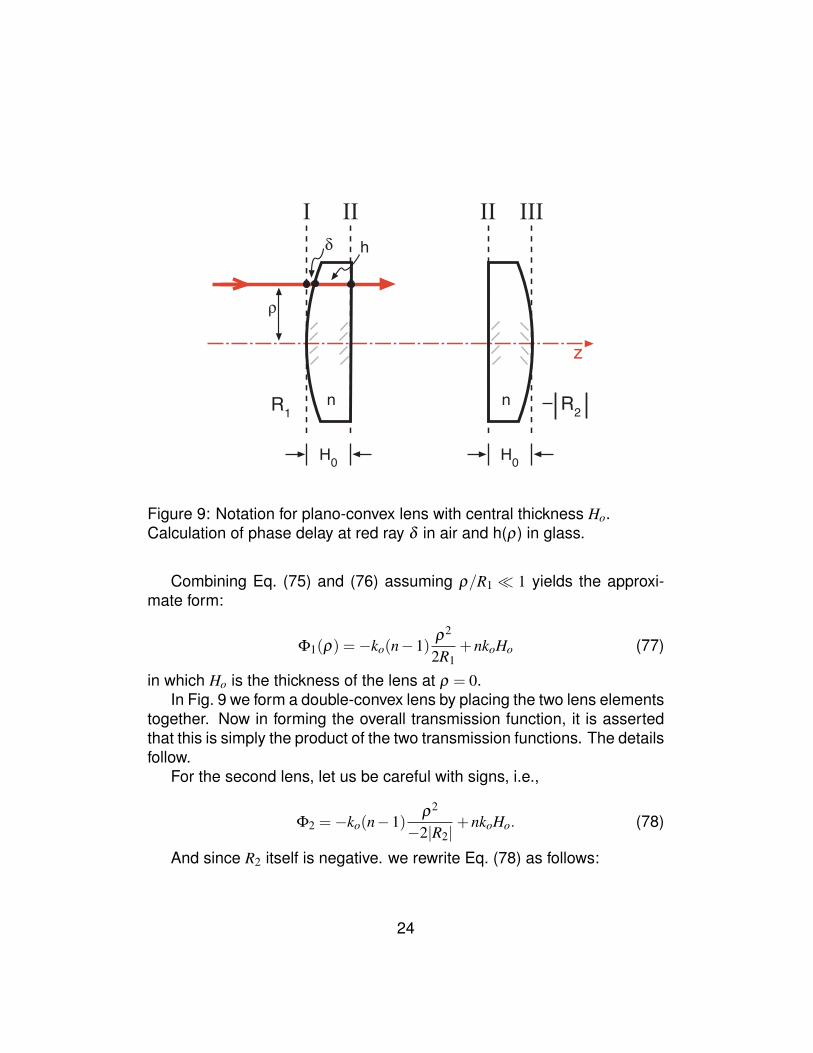
9 Notation for plano-convex lens with central thickness Ho. Calculation ofphase delay at red ray δ in air and h(ρ) in glass. . . . . . . . . . . . . . . . 24

10 Transmission function for imaging the point source with an asphere, seeEqs. (82) to (85) . . . . . . . . . . . . . . . . . . . . . . . . . . . . . . . . . 26

11 Aspheric lens Φ(ρ) between planes I - II with plane wave incident. Ray (a)has an effective focal length shown as z. . . . . . . . . . . . . . . . . . . . . 28

12 Cascade of 4 lenses for imaging input to plane 5. This is a central topic inFourier optics to compute the impulse response p05 for the cascade . . . . 31

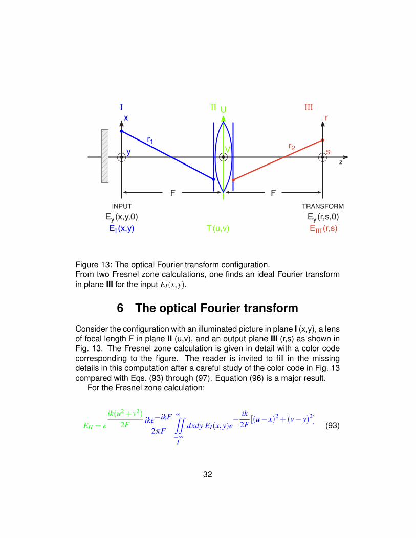
13 The optical Fourier transform configuration. From two Fresnel zone calcu-lations, one finds an ideal Fourier transform in plane III for the input EI(x,y). 32

14 The basis of diffraction-pattern-sampling for pattern recognition in optical-electronic processors is summarized in 4 rules . . . . . . . . . . . . . . . . 34

15 Rapid, millisecond testing of quality of sharpness of hypodermic needles(2.5 billion needles per year) is accomplished with the ring-sedge opticaltransform hybrid: (left) excellent quality; poor needle; poor transform. . . . . 36

16 The 4-F optical processing provides both an idealized space-invariant im-age as well as a perfect optical Fourier transform. It is useful both in theo-retical calculations and in laboratory. . . . . . . . . . . . . . . . . . . . . . . 39

iii

1 Introduction to electromagnetic waves andFourier optics

The foundations of the subject of Fourier Optics rest on Maxwell’s equa-tions, the early studies of interference and interferometry, coherence, andimaging. Important advances in the mathematics of transform theory lead-ing to communication theory from 1900 to the present greatly aided ourunderstanding of these phenomena; the general notion of signal represen-tations such as HTD exp(iωt) herein, and the Fourier transform for optics,and the Laplace transform for electronic circuits. Professor P. M. Duffieuxauthored “L’integral de Fourier et ses applications a l’optique”, MassonEditeur, Paris, 1970 with first editions going back to the early forties. “Itrepresents the first book-length treatment of what is now called Fourieroptics” [1]. At the (1970) meeting of the International Symposium on theapplications of Holography (ICO) in Bescancon, at a Medal awarding ad-dress, Dr. Duffieux told a charming story of how a mathematics professorand colleague had told him about the Fourier transform when PMD showedhim some integral forms he had derived in study of the earlier work of ErnstAbbe.

Interestingly the technological advances in monochromatic sources inelectronics, particularly radio and microwave from 1900 to 1950 lead togreatly enhanced theoretical studies and many now-classic textbooks, ap-peared using HTD of amplitudes.

In optics intensity based considerations were more commonly employed.A notable exception is the brilliant advances in coherence theory leadingto phase contrast microscopy. However, in Optics this situation changesdramatically with the invention and development of holography and nearlymonochromatic lasers. The theoretical treatment and understanding ofthese novel devices were greatly aided by the appearance of now classictextbooks on Fourier Optics [2, 3].

This article contains a modern complete theoretical treatment of FourierOptics based on Maxwell’s equations and current signal representations,as devised from the subject of communication theory.

1

1.1 Maxwell’s equations in real-valued form

The basic equations of electromagnetic theory are briefly reviewed for asimple linear medium so that the signal representation herein can be care-fully explained. In this first section, we describe the time-varying real-valued electric field vector E(r, t) and the time-varying magnetic field vec-tor H(r, t) in Eq. (1) Faraday’s Law and Eq. (2) the generalized Ampere’scircuit law including Maxwell’s electric displacement term. Undergraduatelevel derivation of these first six differential equations of electrodynamicsand their application across the electromagnetic spectrum appear in manytexts, e.g., [4] Griffiths. This article is written using the SI/mks system ofunits. The time-dependent real-valued functions are related as given inEqs. (1) through (6):

∇×E(r, t) =−∂B(r, t)∂ t

(1)

∇×H(r, t) =J (r, t)+∂D(r, t)

∂ t(2)

∇•D(r, t) = ρ(r, t) (3)∇•B(r, t) = 0 (4)

∇•J (r, t) =− ∂∂ t

ρ(r, t) (5)

∇×∇×E(r, t)+µε∂ 2

∂ t2E(r, t) =−µ∂∂ t

J (r, t) (6)

The field vectors are written in boldface type and the common symbolsare used for divergence (∇•) and curl (∇×). Restricting the media to simpledielectrics, the constitutive parameters for permittivity ε and permeabilityµ also give us

B = µH (7)and D = εE (8)

An exact solution of Maxwell’s equations is obtained when one hasE(r, t) and H(r, t) that satisfy Eqs. (1) and (2). Other paths to exact solu-tions are to obtain E(r, t) from Eq. (6) and then use Eqs. (1) and (7) to findH(r, t). Finally, one can introduce any of a variety of vector potentials thathave been developed for particular cases.

2

1.2 Fourier analysis in three dimensions

Consider a scalar function g(x,y, t) with two transverse spatial coordinatesand one temporal coordinate. Now define the Fourier transform G( fx, fy;ν)by the following equation:

G( fx, fy;ν) =∞∫∫∫

−∞

g(x,y, t)e−i2π( fxx+ fyy+νt)dxdydt (9)

It is a straightforward exercise to show that the inversion expression isgiven by Eq. (10):

g(x,y, t) =∞∫∫∫

−∞

G( fx, fy;ν)ei2π( fxx+ fyy+νt)d fxd fydν (10)

This notation and sign convention is used throughout this paper. It isparticularly convenient since the sign of the exponents in the transformkernel are all negative while those of the inversion are all positive.

1.3 Maxwell’s differential equations in temporal trans-form form

In Sec. 1.2, the notation for Fourier analysis in three dimension has beenpresented in order to place in evidence the sign convention to be used.Now, however, we use the obvious form for the temporal transform alone,since we wish to compare the resultng equations to “standard” HTD ex-pressions.

Important integral solutions of Maxwell’s equations are readily obtainedusing temporal Fourier transform forms of Eqs. (1) (2) and (6) with thecorresponding results in Eqs. (11) , (12) and (13) , (14) directly below:

∇×E(r;ν) =−iωµH(r;ν) (11)∇×H(r;ν) = J(r;ν)+ iωεH(r;ν) (12)

∇×∇×E(r;ν)−ω2µεE(r;ν) =−iωµJ(r;ν) (13)

(∇2 + k2)E(x,y,z) = 0 (14)

Equation (14) is valid in a source free region.

3

Now these temporal transform equations are exact and rigorous for opti-cal sources which are transient. Since temporal frequency ν is a variable,solving the above equations gives us a new path to solving problems inwhich there are broadband sources or multi-tone spectra.

Ex(x,y,z; t) (1)

1

Ex(x,y,z;ν) (1)

1

Vx( fx, fy;z;ν) (1)

1

Fxyt (1)

1

Ft (1)

1

Fxy (1)

1

(or htd e+i2πνt) (1)

1

∇×E = −i2πνB (1)

1

(∇2 + k2)Ex(x,y,z;ν) = 0 (1)

1

∇×E = −∂B(r, t)∂ t

(1)

∇2Ex = µε∂ 2Ex

∂ t2 (2)

1

∂ 2Vx

∂ z2 +�k2 − (2π fx)

2 − (2π fy)2�Vx = 0 (1)

1

Vx( fx, fy;z;ν) =

∞��

−∞

dxdy Ex(x,y,z;ν)e−i2π fxx− i2π fyy (1)

Ex(x,y,z;ν) =

∞��

−∞

d fxd fy Vx( fx, fy;z;ν)e+i2π fxx+ i2π fyy (2)

1

�−−−e−i2πνtdt

1

Figure 1: Signal representations in Electromagnetic Waves and FourierOptics

In order to place emphasis on the significance of the result to be in-ferred from Eqs. (11) through (14), let us observe that Eqs. (11) and (12)are simply and precisely the harmonic-time-dependence differential equa-tions for an electromagnetic wave. The reader is cautioned , however, thatour Eq. (9) notation is consistent with an exp(iωt) as in ref. [6].

In Fig. 1 we show the signal representations being used in Sections 1.1and 1.2 in more detail than is necessary for the paper at hand. However,we wanted to show the more general usage including angular spectrum aswell as statistical optics in order to explain our preference for the exp(+iωt)

4

in the HTD representation and its consistency with our Fourier transformnotation.

2 Propagation into the right-half-space

Maxwell’s equations give us the means to obtain exact solutions of manyoptics problems. Both the Hertzian electric dipole and the magnetic dipoleare significant and important and covered in many textbooks [5] - [7]. Inoptics, diffraction theory topics such as propagation through screens, slits,and various apertures were studied extensively for several hundred years.Also lens trains formed by a cascade of lenses along an optical axis is acommon configuration, as in Sec. 5.

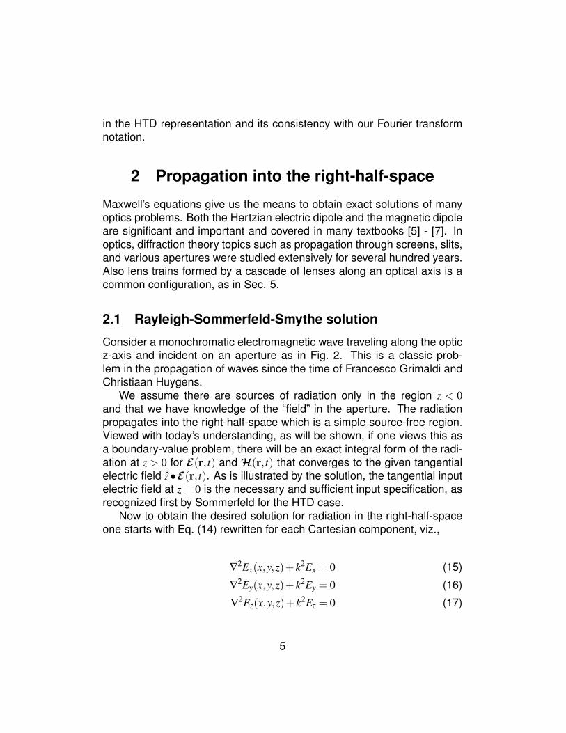
2.1 Rayleigh-Sommerfeld-Smythe solution

Consider a monochromatic electromagnetic wave traveling along the opticz-axis and incident on an aperture as in Fig. 2. This is a classic prob-lem in the propagation of waves since the time of Francesco Grimaldi andChristiaan Huygens.

We assume there are sources of radiation only in the region z < 0and that we have knowledge of the “field” in the aperture. The radiationpropagates into the right-half-space which is a simple source-free region.Viewed with today’s understanding, as will be shown, if one views this asa boundary-value problem, there will be an exact integral form of the radi-ation at z > 0 for E(r, t) and H(r, t) that converges to the given tangentialelectric field z•E(r, t). As is illustrated by the solution, the tangential inputelectric field at z = 0 is the necessary and sufficient input specification, asrecognized first by Sommerfeld for the HTD case.

Now to obtain the desired solution for radiation in the right-half-spaceone starts with Eq. (14) rewritten for each Cartesian component, viz.,

∇2Ex(x,y,z)+ k2Ex = 0 (15)

∇2Ey(x,y,z)+ k2Ey = 0 (16)

∇2Ez(x,y,z)+ k2Ez = 0 (17)

5

(x′,y′,0)

(x,y,z ≥0)

R1x

y

z

Figure 2: Radiation into the right-half-space from a circular aperture in thez = 0 plane

Now consider the use of a Green’s function solution using either Eq. (15)or (16), as follows. We write

Gs(∇2 + k2)Ex = 0 (18)

Ex(∇2 + k2)Gs =−δ (r− r′)Ex (19)

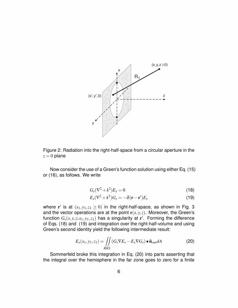
where r′ is at (x1,y1,z1 ≥ 0) in the right-half-space, as shown in Fig. 3and the vector operations are at the point r(x,y,z). Moreover, the Green’sfunction Gs(x,y,z;x1,y1,z1) has a singularity at r′. Forming the differenceof Eqs. (18) and (19) and integration over the right-half-volume and usingGreen’s second identity yield the following intermediate result:

Ex(x1,y1,z1) =∫∫

RHS

(Gs∇Ex−Ex∇Gs)• noutdA (20)

Sommerfeld broke this integration in Eq. (20) into parts asserting thatthe integral over the hemisphere in the far zone goes to zero for a finite

6

aperture source (see Eq. (22) below).

r(x,y,z)

R1

x

yz

R2

r′(x1,y1,z1)r″(x1,y1,_z1)

Figure 3: Notation in the calculationfor Sommerfeld’s Green’s functionwith a δ -function at point r′(x1,y1,z1)in the right-half-space.

R1

x

yz

R2

r′r″

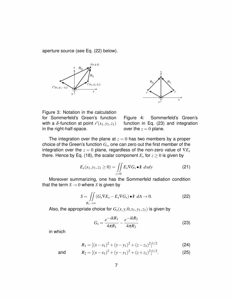
Figure 4: Sommerfeld’s Green’sfunction in Eq. (23) and integrationover the z = 0 plane.

The integration over the plane at z = 0 has two members by a properchoice of the Green’s function Gs, one can zero out the first member of theintegration over the z = 0 plane, regardless of the non-zero value of ∇Exthere. Hence by Eq. (18), the scalar component Ex for z≥ 0 is given by

Ex(x1,y1,z1 ≥ 0) =∫∫

z=0

Ex∇Gs • z dxdy (21)

Moreover summarizing, one has the Sommerfeld radiation conditionthat the term S→ 0 where S is given by

S =∫∫

R1→∞

(Gs∇Ex−Ex∇Gs)• r dA→ 0. (22)

Also, the appropriate choice for Gs(x,y,0;x1,y1,z1) is given by

Gs =e−ikR1

4πR1− e−ikR2

4πR2(23)

in which

R1 = [(x− x1)2 +(y− y1)

2 +(z− z1)2]1/2 (24)

and R2 = [(x− x1)2 +(y− y1)

2 +(z+ z1)2]1/2. (25)

7

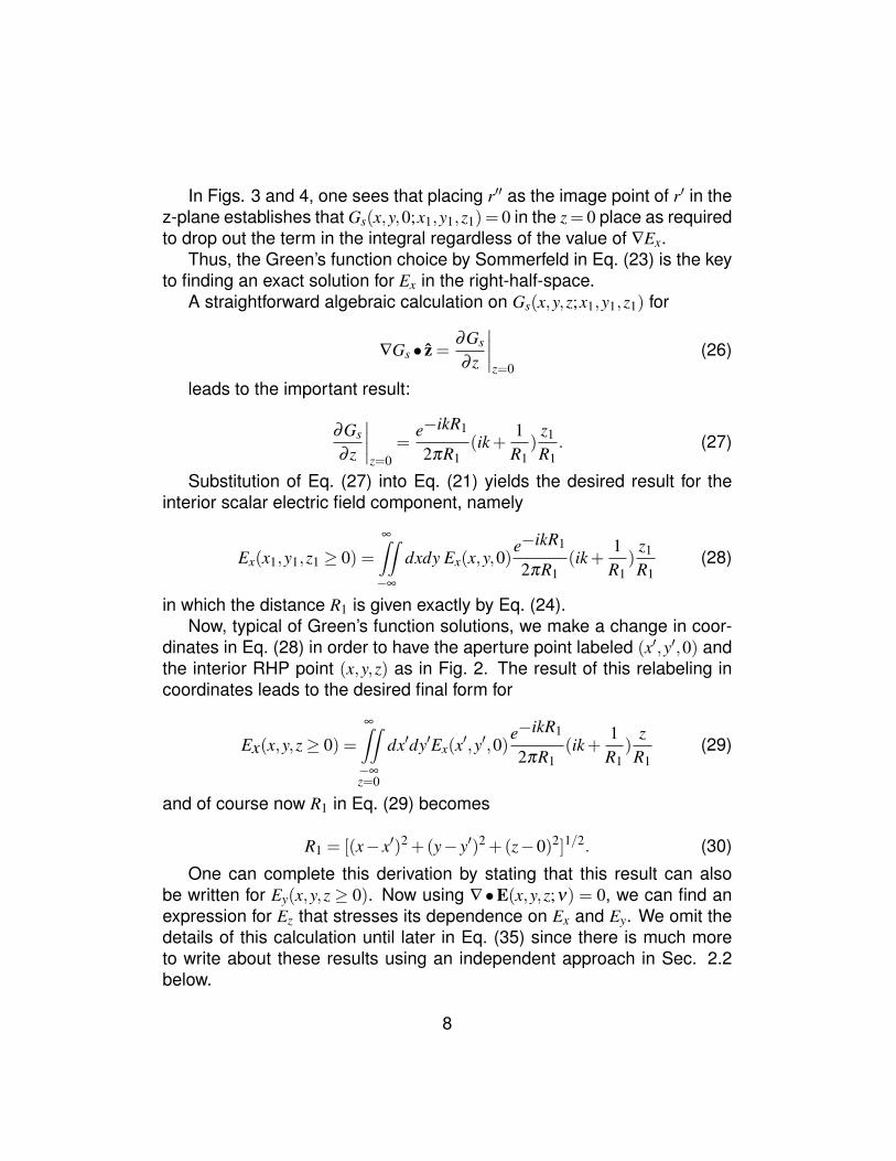
In Figs. 3 and 4, one sees that placing r′′ as the image point of r′ in thez-plane establishes that Gs(x,y,0;x1,y1,z1)= 0 in the z= 0 place as requiredto drop out the term in the integral regardless of the value of ∇Ex.

Thus, the Green’s function choice by Sommerfeld in Eq. (23) is the keyto finding an exact solution for Ex in the right-half-space.

A straightforward algebraic calculation on Gs(x,y,z;x1,y1,z1) for

∇Gs • z =∂Gs

∂ z

∣∣∣∣z=0

(26)

leads to the important result:

∂Gs

∂ z

∣∣∣∣z=0

=e−ikR1

2πR1(ik+

1R1

)z1

R1. (27)

Substitution of Eq. (27) into Eq. (21) yields the desired result for theinterior scalar electric field component, namely

Ex(x1,y1,z1 ≥ 0) =∞∫∫

−∞

dxdy Ex(x,y,0)e−ikR1

2πR1(ik+

1R1

)z1

R1(28)

in which the distance R1 is given exactly by Eq. (24).Now, typical of Green’s function solutions, we make a change in coor-

dinates in Eq. (28) in order to have the aperture point labeled (x′,y′,0) andthe interior RHP point (x,y,z) as in Fig. 2. The result of this relabeling incoordinates leads to the desired final form for

Ex(x,y,z≥ 0) =∞∫∫

−∞z=0

dx′dy′Ex(x′,y′,0)e−ikR1

2πR1(ik+

1R1

)z

R1(29)

and of course now R1 in Eq. (29) becomes

R1 = [(x− x′)2 +(y− y′)2 +(z−0)2]1/2. (30)

One can complete this derivation by stating that this result can alsobe written for Ey(x,y,z ≥ 0). Now using ∇ •E(x,y,z;ν) = 0, we can find anexpression for Ez that stresses its dependence on Ex and Ey. We omit thedetails of this calculation until later in Eq. (35) since there is much moreto write about these results using an independent approach in Sec. 2.2below.

8

2.2 Impulse response for propagation into the RHS

In linear optical systems a topic of central interest is to derive an exactimpulse response for propagation into the right-half-space (RHS). In Sec.2.1 Eq. (29) is presented as a rigorous solution of Maxwell’s equation forthis impluse response. It is applicable over the entire range that Maxwell’sequations holds from near field optics to telescopes. Hence, in this articleit seemed worthwhile to develop an independent derivation of Eq. (29) andrelated material.

Again consider the setup and notation in Figs. 2 for radiation into theRHS. Smythe was at least early to write out a detailed existence theoremfor electromagnetic waves in a closed source-free region, and he stressedthe necessary and sufficient need for either the tangential electric field orthe tangential magnetic field, although he did not explicitly cover a regionsuch as the RHS [8]. Also Smythe was first to write the complete exactsolution for the right-half-space problem in an entirely vector form in hisfamous Phys. Rev. (1947) paper [9]. The vector result for the internal fieldis given in Fourier optics or HTD form as follows:

E(r;ν) =1

2π∇×

∫∫

z′=0

z′×E(r′)e−ikR1

R1dx′dy′ (31)

in which the free-space Green’s function G is appropriate as follows:

G(r,r′) =e−ikR1

4πR1, (32)

and E(r′) at (x′,y′,0) is the final field in the aperture.Let me describe some illuminating illustrative exercises for the dedi-

cated reader. Derive the equations below in Eq. (33) to (35) for the com-ponents.

To verify that this result in Eq. (31) is an exact solution for Maxwell’sequations, one needs to verify that the vector E(r;ν) is a solution of thevector wave equation (13) or (14).

It is fascinating to see the impulse responses for propagation into theRHS for a simple medium. There is no “mixing” of the x and y polariza-tions. Moreover, both the Ex and Ey are seen to contribute to the Ez com-ponent. This illustrates very nicely the existence theorem for this situation

9

and Maxwell’s equations. For the RHS problem, one can supply any rea-sonable functions for the tangential components Ex and Ey (necessary andsufficient) but any more will likely lead to inconsistent results.

2.3 Summary of impulse response

2.3.1 The Right-Half-Space

Here are the exact solutions of Maxwell’s equations for propagation in theright-half-space.

The Rayleigh-Sommerfeld-Smythe formulas:

Ex(x,y,z) =∞∫∫

−∞

dx′dy′Ex(x′,y′,0)e−ikR1

2πR1(ik+

1R1

)z

R1(33)

Ey(x,y,z) =∞∫∫

−∞

dx′dy′Ey(x′,y′,0)e−ikR1

2πR1(ik+

1R1

)z

R1(34)

Ez(x,y,z) =∞∫∫

−∞

dx′dy′{Ex(x′,y′,0)x′− x

R1+Ey(x′,y′,0)

y′− yR1}e−ikR1

2πR1(ik+

1R1

)

(35)

Another exact, useful and readily proven result for the RHS is given by[10]:

Ex,y(x,y,z) =−∂∂ z

∞∫∫

−∞

dx′dy′Ex,y(x′,y′,0)e−ikR1

2πR1(36)

They are valid for z≥ 0, and R1 is given by Eq. (30), Fig. 2.Many scientists have contributed to an understanding of interference

patterns arising as light propagates, e.g., from two pinholes, through anopen aperture, or from an array of coherent sources. Huygens’ princi-ple stated more than three hundred years ago in the description of thepropagation of a wavefront is among the earliest major contributions. Hisasserions are in accord with the theory which we have presented.

For us, today, using Maxwell’s equations and the formula presented onthe previous page, we can see that a diffraction pattern is made up by the

10

superposition of radiation from differential elements given by

dx′dy′Ex(x′,y′,0).

These give rise to “secondary waves” which are traveling in the right-half-space with a very weak angular dependents given by the term z/R1.The superposition weighting is given precisely in amplitude and phase bythe term:

e−ikR1

2πR1(ik+

1R1

)z

R1

All of the physical details of interference patterns are contained in theseformulas for the radiation in the right-half-space resulting from a givenaperture distribution.

2.3.2 The full 4π-steradian space

In the classic text on electromagnetic wave by Papas [5], there is an ex-cellent treatment of radiation from monochromatic sources in unboundedregions, i.e., 4π steradians. He describes two methods of solution: vectorpotentials and the dyadic Green’s function. While our emphasis for opticsis on the right-half-space topic, it is important to mention this basic resultfor the impulse response for the 4π-steradian or full-space case.

For the same simple medium with constitutive parameters µ, ε, onehas the same group of Maxwell’s equations as our Eqs. (11), (12).

The magnetic vector potential A is defined by

B = ∇×A. (37)

Hence, by Eq.Eq. (11), one can write the E field as

E =−iωA−∇φ . (38)

With the choice of the Lorenz gauge relating A and φ , namely that

∇•A+ iωεµφ = 0 (39)

one can write a wave equation as follows:for the vector potential A(r;ν):

11

∇2A+ k2A =−µJ. (40)

Presenting a Green’s function solution, Papas derives the integral equa-tion solution for the radiation into free space, 4π-steradians:

A(r) =∞∫∫∫

−∞

dx′dy′dz′J(r′)e−ikR1

4πR1(41)

Equation (41) is the basis equation for radiation of electromagnetic wavesinto free space in a spherical configuration. It is particularly useful for ra-diation of current sources as given by J(r′,ν) where the R1 is given by

R1 = [(x− x′)2 +(y− y′)2 +(z− z′)2]1/2 (42)

It is important to understand these two distinct radiation problems. Theyare often confused. First, one has the scalar electric field componentspropagating into the right-half-space expressed in terms of source-termsin the plane at z = 0. The solutions are given in Eqs. (33) to (36).

Secondly, in the radiation into 4π-space, we have the vector potentialA(r;ν) resulting from source currents J(r′;ν), and the resulting impulseresponse given by the free-space Green’s function in Eq. (41).

3 Optical diffraction illustrations

The theory of Fourier Physical Optics as presented in the earlier sectionsof this article is based on Maxwell’s equations. The precision possible withrigorous or exact solutions of electromagnetic theory is discussed in somedetail in Jackson [11]. This enormous range includes wavelength or fre-quency from fractional cycles per second to ultraviolet and of course DC.It includes power range from 10−20 watts to many megawatts. It also in-cludes subpulse propagation as well as µµsec transients. Many new fields

12

are developing in optics such as computational imaging that are permittingthe solution of many boundary value problems, and near-field optics prob-lems that were considered inaccessible until rather recently.

3.1 The circular aperture

For a first illustration, it is helpful to start with an important problem inwhich a theoretical approach leads to interesting results [10]. Consider aperfectly conducting, infinitesimally thin conducting plane sheet containinga circular aperture of radius (a) placed in the (x,y) plane at z = 0, as shownin Fig. 5. It is illuminated by a plane-polarized monochromatic plane wavewith wave number k = 2π/λ where λ � a so boundary effects can be ig-nored. Clearly, Eq. (33) or (36) can be used. Let us restrict our solutionto the optic axis z so that we gain an understanding of the different zonesshown. Hence, for a fixed amplitude Eo of the scalar component of electricfield, by Eq. (36), one can write the field along the optical axis Ex(0,0,z;ν)as

(x′,y′,0)

R1

x

z

(x,y,z)

R0

NZ FZ FAR

2a

0

Figure 5: Uniformly illuminated circular aperture of radius (a) is calculatedon axis to provide clear picture of (NZ) near field, (FZ) Fresnel zone andthe FAR-zone. [10]

13

Ex(0,0,z≥ 0) =− ∂∂ z

∫∫

A

dx′dy′Ex(x′,y′,0)e−ikR1

2πR1, (43)

in which the illumination is given in polar coordinates, viz.

Ex(x′,y′,0) = Eocirc(ρ/a), ρ = [x′2 + y′2]1/2 (44)

and the distance R1 given in polar form is

R1 = [ρ2 + z2]1/2. (45)

Equation (43) is rewritten to yield:

Ex(0,0,z≥ 0) =−Eo∂∂ z

a∫

0

e−ik(ρ2 + z2)1/2

(ρ2 + z2)1/2 2πρdρ. (46)

This can be integrated exactly to yield the result:

Ex(0,0,z≥ 0) = Eo{e−ikz− zd

e−ikd} (47)

where

d =√

a2 + z2. (48)

First as expected, when z→ 0, the radiation field at the aperture re-duces to the input Eo. As described in Sec. 2.2, this result is consistentwith the existence theorem for Maxwell’s equations, Eqs. (1) through (4),extended to the right-half-space and adding Sommerfeld radiation condi-tion, given by Eq. (22). We see that specification of HTD together with thetangential electric field at the input plane z = 0.

By Eq. (34) one sees that Ey(x,y,z≥ 0) is identically zero as expected.And of course, one can calculate Ez by Eq. (35) clearly dependent on thenon-zero tangential electric field, Ex, input.

In order to study the z-dependence of Ex further, it is interesting to thinkof the calculation as in the HTD signal representation. By Eqs. (47) and(48), one can insert the time dependence simply as follows:

Ex(0,0,z; t) = Eo{e−ikz− z√z2 +a2

e−ik√

z2 +a2}e+i2πνt . (49)

14

LOG (Z) (Z IN mm)

AXIA

L FI

ELD

STR

ENG

TH S

QUA

RED

FRES

NEL

REG

ION

FAR

ZO

NE

5.0

4.0

3.0

2.0

1.0

0.0-3 -2 -1 0 1 2 3 4 5

Figure 6: Axial field strength squared w(z) vs log(z) for uniformly illumi-nated circular aperture, as in Eq. (51) The dashed lines are the envelopeof w(z). The actual value of w(z) is plotted in red in the Fresnel zone forthe first few cycles, but it is too fine scalar to plot accurately.

In order to monitor the optical field along the optical axis, one can usea single photodiode or a CMOS detector array. Hence, in our illustrativestudy, we will use energy density in the Ex electric field. Hence, we definew as follows

w(z) = |Ex(0,0,z : t)|2. (50)

Hence combining Eq. (47) and (48) with some algebra yields the fol-lowing form:

w(z) = |Eo|2{1+z2

z2 +a2 −2z√

z2 +a2cosk[

√z2 +a2− z]} (51)

in which k = 2π/λ .No approximations have been made in deriving Eq. (51) for the squared

electric field component Ex from the initial solution in Eq. (47). Hence, it is

15

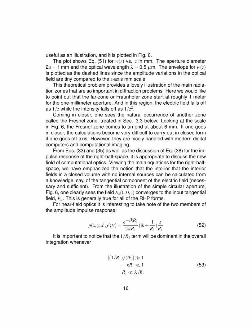
useful as an illustration, and it is plotted in Fig. 6.The plot shows Eq. (51) for w(z) vs. z in mm. The aperture diameter

2a = 1 mm and the optical wavelength λ = 0.5 µm. The envelope for w(z)is plotted as the dashed lines since the amplitude variations in the opticalfield are tiny compared to the z-axis mm scale.

This theoretical problem provides a lovely illustration of the main radia-tion zones that are so important in diffraction problems. Here we would liketo point out that the far-zone or Fraunhofer zone start at roughly 1 meterfor the one-millimeter aperture. And in this region, the electric field falls offas 1/z while the intensity falls off as 1/z2.

Coming in closer, one sees the natural occurrence of another zonecalled the Fresnel zone, treated in Sec. 3.3 below. Looking at the scalein Fig. 6, the Fresnel zone comes to an end at about 6 mm. If one goesin closer, the calculations become very difficult to carry out in closed formif one goes off-axis. However, they are nicely handled with modern digitalcomputers and computational imaging.

From Eqs. (33) and (35) as well as the discussion of Eq. (38) for the im-pulse response of the right-half-space, it is appropriate to discuss the newfield of computational optics. Viewing the main equations for the right-half-space, we have emphasized the notion that the interior that the interiorfields in a closed volume with no internal sources can be calculated froma knowledge, say, of the tangential component of the electric field (neces-sary and sufficient). From the illustration of the simple circular aperture,Fig. 6, one clearly sees the field Ex(0,0,z) converges to the input tangentialfield, Eo. This is generally true for all of the RHP forms.

For near-field optics it is interesting to take note of the two members ofthe amplitude impulse response:

p(x,y;x′,y′;ν) =e−ikR1

2πR1(ik+

1R1

)z

R1(52)

It is important to notice that the 1/R1 term will be dominant in the overallintegration whenever

|(1/R1)/(ik)| � 1kR1� 1

R1� λ/8.(53)

16

In the illustration of the circular aperture, of course both terms are in-cluded in the calculation. An advanced and comprehensive treatment ofthe theory of diffraction is provided by Born and Wolf [12].

3.2 The far-zone

Now starting with a more general aperture shape in the z = 0 plane of Fig.2, we consider that an x-plane polarized scalar electric field Ex(x′,y′,0;ν) isused as the illustration. Hence, we seek an approximate, more integrableform of the exact Eq. (33) that is repeated as Eq. (54), i.e.,

Ex(x,y,z : ν) =∞∫∫

−∞

dx′dy′Ex(x′,y′,0)e−ikR1

2πR1(ik+

1R1

)z

R1(54)

The far-zone, also known as the Fraunhofer region, is characterized bylarge values of R1. Mainly in this treatment, we would like carefully to pointout the conventional theoretical assumptions in the integration of Eq. (33)or (54) in the far-zone region.

In the far-zone calculation, however, the situation is vastly different rel-ative to accuracy for exp(−ikR1). The phase term needs to be accurate tothe order of ±π/8 no matter how large Ro is. For example, if you are mak-ing measurements at 10 m with an optical wavelength of 0.5 µm, the kRois the order of 4π×107 radians; and the tolerance error in R1 is fractionallywell below one part in 107.

Hence, in the far-zone, Eq. (54) can be approximated by

Ex(x,y,z;ν) =ik

2πRo

( zRo

) ∞∫∫

−∞

dx′dy′Ex(x′,y′,0)e−ikR1 (55)

For the illustration problem, consider an open rectangular aperture thatis Lx by Ly length in the conducting metallic sheet at z = 0. We take Lx,y > λso that we can study the patterns from slits to large square apertures.Using the notation in Fig. 5, we already understand that the distance Ro�λ so only the ik member in Eq. (54) remains for the far-zone.

Moreover, amplitude terms that are approximated in this integrationwill cause errors in percentage that are roughly that of the approximation.Hence if a five-percent accuracy solution is sought, then amplitude termsneed only be accurate to five-percent.

17

For the R1 in the phase term (−ikR1), we write

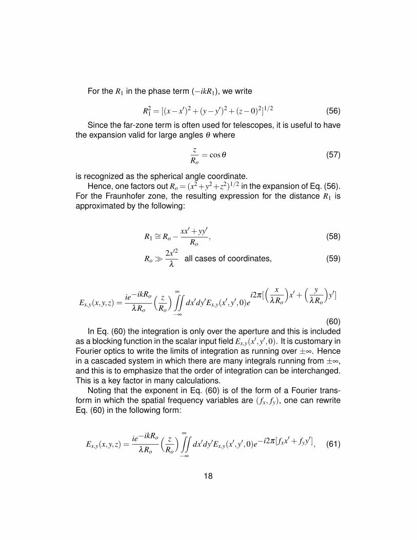
R21 = [(x− x′)2 +(y− y′)2 +(z−0)2]1/2 (56)

Since the far-zone term is often used for telescopes, it is useful to havethe expansion valid for large angles θ where

zRo

= cosθ (57)

is recognized as the spherical angle coordinate.Hence, one factors out Ro =(x2+y2+z2)1/2 in the expansion of Eq. (56).

For the Fraunhofer zone, the resulting expression for the distance R1 isapproximated by the following:

R1 ∼= Ro−xx′+ yy′

Ro, (58)

Ro�2x′2

λall cases of coordinates, (59)

Ex,y(x,y,z) =ie−ikRo

λRo

( zRo

) ∞∫∫

−∞

dx′dy′Ex,y(x′,y′,0)ei2π[

( xλRo

)x′+

( yλRo

)y′]

(60)In Eq. (60) the integration is only over the aperture and this is included

as a blocking function in the scalar input field Ex,y(x′,y′,0). It is customary inFourier optics to write the limits of integration as running over ±∞. Hencein a cascaded system in which there are many integrals running from ±∞,and this is to emphasize that the order of integration can be interchanged.This is a key factor in many calculations.

Noting that the exponent in Eq. (60) is of the form of a Fourier trans-form in which the spatial frequency variables are ( fx, fy), one can rewriteEq. (60) in the following form:

Ex,y(x,y,z) =ie−ikRo

λRo

( zRo

) ∞∫∫

−∞

dx′dy′Ex,y(x′,y′,0)e−i2π[ fxx′+ fyy′], (61)

18

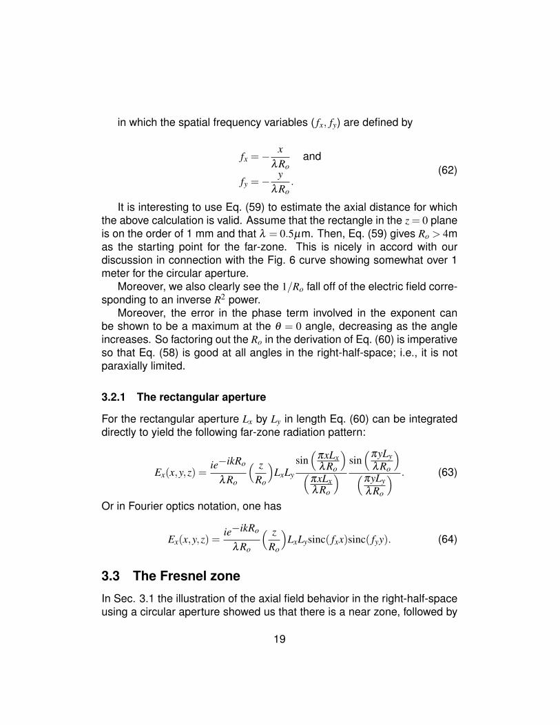
in which the spatial frequency variables ( fx, fy) are defined by

fx =−x

λRoand

fy =−y

λRo.

(62)

It is interesting to use Eq. (59) to estimate the axial distance for whichthe above calculation is valid. Assume that the rectangle in the z = 0 planeis on the order of 1 mm and that λ = 0.5µm. Then, Eq. (59) gives Ro > 4mas the starting point for the far-zone. This is nicely in accord with ourdiscussion in connection with the Fig. 6 curve showing somewhat over 1meter for the circular aperture.

Moreover, we also clearly see the 1/Ro fall off of the electric field corre-sponding to an inverse R2 power.

Moreover, the error in the phase term involved in the exponent canbe shown to be a maximum at the θ = 0 angle, decreasing as the angleincreases. So factoring out the Ro in the derivation of Eq. (60) is imperativeso that Eq. (58) is good at all angles in the right-half-space; i.e., it is notparaxially limited.

3.2.1 The rectangular aperture

For the rectangular aperture Lx by Ly in length Eq. (60) can be integrateddirectly to yield the following far-zone radiation pattern:

Ex(x,y,z) =ie−ikRo

λRo

( zRo

)LxLy

sin(πxLx

λRo

)

(πxLxλRo

)sin(πyLy

λRo

)

(πyLyλRo

) . (63)

Or in Fourier optics notation, one has

Ex(x,y,z) =ie−ikRo

λRo

( zRo

)LxLysinc( fxx)sinc( fyy). (64)

3.3 The Fresnel zone

In Sec. 3.1 the illustration of the axial field behavior in the right-half-spaceusing a circular aperture showed us that there is a near zone, followed by

19

a Fresnel zone, and then at larger distances the far-zone. In Sec. 3.2 forthe far-zone, we illustrated the theory and a careful calculation that wasdemonstrated to be good in the right-half-space when the overall rangedistance Ro � 2x2/λ . Numerically, we estimated that for small millimeterapertures, one can calculate accurate patterns when Ro & 4 m. We as-serted that the calculation is excellent at all angles. This calculation is aneasy extension of the material presented.

However, one very important calculation in Fourier optics is to treatlenses, either a single lens or a cascade of lenses. In this Sec. 3.3 wedescribe the Fresnel-zone calculation. It is very important since it can beused to handle lens cascades where the spacing is generally much smallerthan in the far-zone. As shown for the circular aperture, Figs. 5 and 6,hopefully we are dealing with several millimeters rather than meters.

For the Fresnel zone, the theory proceeds as in Sec. 3.2. First forEq. (33), we need to establish an expansion for the phase term. Using thenotation as in Fig. 5, the exact expression for the distance R1 is given by

R1 = [(x− x′)2 +(y− y′)2 +(z−0)2]1/2. (65)

Factoring z and using the binomial expansion gives the following form:

R1 ∼= z+(x− x′)2 +(y− y′)2

2z. (66)

Factoring with removal of z and leaving (x,y) in the series limits one toa paraxial solution. It is better, however, with regard to axial distance, i.e.,valid much closer-in. The limitation on primed coordinates (all cases) ischaracterized by the following:

z3 &(x− x′)4

2λ. (67)

For a 1 mm aperture, this gives an axial distance z ≈ 10 mm whenλ = 0.5µm. For the Fresnel zone case, Eq. (33) can rewritten as

20

Ex(x,y,z;ν) =iz

λR2o

∞∫∫

−∞

dx′dy′Ex(x′,y′,0)e−ikR1 , (68)

Ex(x,y,z;ν) =ie−ikz

λ z

∞∫∫

−∞

dx′dy′Ex(x′,y′,0)e− iπ

λ z[(x− x′)2 +(y− y′)2]

. (69)

In many instances of lens design using modern digital computers, onecan use Eq. (68) with the exact exponential. However, Eq. (69) is thestandard form for a Fresnel calculation. The reader is left to use Eq. (67)to predict the starting point for the Fresnel zone region comparing thisestimate to the exact values of the axial field strength as in Fig. 6 fromEq. (51).

4 Transmission function theory for lenses

4.1 Review of simple lens models [2]

Most of the theory relative to the right-half-space topic is concerned withhow wavefronts propagate in this region. However, one of the central prob-lems in Fourier optics is to analyze a cascade of lenses that have beenplaced along an optical axis, say, for the formation of an image or to de-scribe a compound lens. It is important to develop an understanding ofthe operation of lenses and an analytical theory that is useful for wave-fronts. Clearly, too, there is a considerable theory about the design andperformance of lenses, since they date back to our earliest history. Weare careful in the following material to use sign conventions and languagethat is consistent with usage in the field of geometric optics, i.e., first-orderor Gaussian optics. Our simple cases are to have light traveling from leftto right in the positive z-axis direction. Convergent lenses have a positivefocal length f . A glass lens with index of refraction n and two positive radiiis shown in Fig. 7.

A simple thin lens of glass with index of refraction n will have a focallength f given by

1f= (n−1)

( 1R1− 1

R2

), (70)

21

!

n

R1 R2

Figure 7: Convergent lens with R1, R2 positive and a positive focal lengthas in Eq. (70)

where R1 and R2 are radii of spherical end segments, and the lens is usedin air.

Also a point source at s1 in front of the lens will be imaged at a distances′1 given by the lensmaker’s equation:

1s+

1s′1

=1f. (71)

Now in order to bring wavefronts into the picture, as shown in red inFig. 8, consider a plane wave entering the lens which is thicker at theoptic axis than at its edges. For a lens that has a spherical segment, theexiting wavefronts will bend forward as shown. Now the phase delay of theplane wave between planes I and II can be calculated approximately bysumming ∑kl in a straight ray through the plano-convex structure shownhaving positive radius R1 at plane I and an infinite radius at the plane IIexit.

Now defining the amplitude transmission function, T12(ρ), as follows:

T12(ρ) =Scalar electric field exiting (II)

Scalar electric field entering (I)(72)

or

T12(ρ) = e−iΦ1 , (73)

we can sum the phase delays:

22

WAVEFRONTS

RAYS

6π 2π 0

Figure 8: Positive lens with rays (upper) and wavefronts (lower).The converging wavefronts are labelled with phase corresponding to HTDof exp(iωt) dependence

Φ1(ρ) = ko ∑nln (74)

in which n is the glass index of refraction and ko = 2π/λo, where λo is thefree space wavelength.

Assuming a spherical R1 (which can be refined in the next section), onecan write the departure δ as is well-known:

δ = R1−√

R21−ρ2 (75)

Then the phase delay Φ(ρ) is given by

Φ1(ρ) = koδ +nkoh(ρ). (76)

23

z

h

n nR1

ρ

δ

R2

I II IIIII

H0 H0

Figure 9: Notation for plano-convex lens with central thickness Ho.Calculation of phase delay at red ray δ in air and h(ρ) in glass.

Combining Eq. (75) and (76) assuming ρ/R1 � 1 yields the approxi-mate form:

Φ1(ρ) =−ko(n−1)ρ2

2R1+nkoHo (77)

in which Ho is the thickness of the lens at ρ = 0.In Fig. 9 we form a double-convex lens by placing the two lens elements

together. Now in forming the overall transmission function, it is assertedthat this is simply the product of the two transmission functions. The detailsfollow.

For the second lens, let us be careful with signs, i.e.,

Φ2 =−ko(n−1)ρ2

−2|R2|+nkoHo. (78)

And since R2 itself is negative. we rewrite Eq. (78) as follows:

24

Φ2 =−ko(n−1)ρ2

2R2+nkoHo. (79)

Hence, by the defining expression in Eq. (72), we form the product ofthe transmission functions corresponding to Eqs. (77) and (79). Moreover,the thin lens approximation is to set Ho = 0. Hence, the sum of Eqs. (77)and (79) yields the thin lens approximation for the plase delay. The cor-responding transmission function for the double-convex lens is given bysubstitution of Eqs. (77) and eqrefeq79 with Ho = 0 into Eq. (73). Thus, thederivation yields the transmission function as follows:

T (ρ) = eiko

(n−1)2

ρ2( 1R1− 1

R2

)(80)

With the positive lens one needs to have a positive focal length. FromEq. (80) and comparing to Eq. (70), clearly one has

1f= (n−1)

( 1R1− 1

R2

)and

T (ρ) = e+

ikoρ2

2 f .

(81)

Lets look at the sign in Eq. (81). It tells us that the phase of the ”forward-curved” wave in the output is bent forward as is clear from Fig. 8. This signfor the transmission function is in accord with an exp(iωt) notation.

4.2 Generalized transmission function for aspheres

The transmission model for a lens as given in Sec. 4.1 is based on amixture of ray and wave optics. It has the advantage of building a goodphysical understanding of the performance of a lens, but it does not givemuch insight into what would constitute an ideal shape for a lens nor onwhat would lead to a lens of idealized performance. For Fourier opticsone needs a more abstract definition of a lens that is based on diffractiontheory. This formulation also should not be based on the assertion of sim-ple spherical surfaces. With today’s knowledge we understand that someaspherical surface is needed if one is planning excellent performance.

25

F F

I II

DIPOLESOURCE

IMAGE

ρ

s1 s′1

0

Figure 10: Transmission function for imaging the point source with an as-phere, see Eqs. (82) to (85)

For the Fourier optics model, we prefer to start with a result or founda-tion based on Maxwell’s equations. So assume a monochromatic plane-polarized light from a laser of wavelength λ . From Eq. (33) for a deltafunction input point source at a distance s1 from the lens in Fig. 10, onecan immediately write the expanding wavefront at plane I, Ex(ρ) given by

exp(−ik√

s21−ρ2) where apodization is dropped.

Now a few example and some reflection leads one to an answer of thefollowing question. What exiting wavefront will lead to a point source at adistance s′1 from plane II? Of course it will likely be blurred by diffraction.

The answer is that the exiting wavefront from plane II needs to have a

wavefront given by exp(ik√

s′21 +ρ2). Again we have neglected the possi-bility of using apodization.

The transmission function for a lossless aspheric lens T (ρ) is then de-fined with a phase delay or sag factor Φ(ρ), as follows:

26

T (ρ) =Scalar electric field exiting plane IIScalar electric field entering plane I

(82)

T (ρ) = e−iΦ (83)

T (ρ) =e+ik[(s′21 +ρ2)1/2− s′1]

e−ik[(s21 +ρ2)1/2− s1]

, (84)

in which the radius ρ =√

x2 + y2 in the transverse plane as in Fig. 10. Wehave made the lens thin by introducing the subtraction terms s′1 and s1, inthe numerator and denominator, respectively. The transmission of Eq. (84)is expanded in terms powers of (ρ/s′1)

2m and (ρ/s1)2m using G & R: 1.112

to yield

Tb(ρ) = eik

(s′1

[12

( ρs′1

)2− 1

8

( ρs′1

)4+

116

( ρs′1

)6− 5

128

( ρs′1

)8+ · · ·

]+

+s1

[12

( ρs1

)2− 1

8

( ρs1

)4+

116

( ρs1

)6− 5

128

( ρs1

)8+ · · ·

])(85)

Eq. (85) is a complete specification for an asphere in a power seriesexpansion. While a complete discussion of this transmission function isbeyond the scope of this article, more details can found in the literature[13]. Detailed aberration theory references are also cited [12, 14, 15].

4.3 Illustrative design of the tailored asphere

In optical system design it is commonplace to design aspheric lenses us-ing modern digital computer software. Large apertures are readily han-dled. Moreover, a lens specification in terms of phase delay as the φ(ρ)in Eq. (82) to (85) is readily manufactured. This specification based onFourier optics and wavefronts makes an important connection of Fourieroptics to geometric optics or optical system design.

Axicons are lens elements having the property of transforming a pointsource of light into an axial segment, i.e., increasing the depth of field. In

27

such an application one typically has a range of focal lengths to accom-modate, call it f (ρ). If one proposes to create a lens design with a radiallysymmetric aspheric lens, it is necessary to establish an appropriate phasedelay Φ(ρ) and a corresponding transmission function, Ta(ρ) for the lensmaker.

(a)

I II

z

! R1

z

!

Figure 11: Aspheric lens Φ(ρ) between planes I - II with plane wave inci-dent. Ray (a) has an effective focal length shown as z.

In the following paragraphs of this section, we describe the design of anasphere given a desired radial variation in focal length using Fourier opticswavefront notions. More specifically, we wish to establish the relationshipbetween φ(ρ) and the corresponding radially varying focal length f (ρ), as

28

in Fig. 11. This is a basic question.Consider the asphere is between planes I, II. A plane polarized plane

wave in incident. Rays at different heights are refracted to the optical axiscrossing at different values z for each ray. Clearly the problem is ideallysuited to our Rayleigh-Sommerfeld-Smythe formulation.

Choosing Eq. (33) and recognizing that the phase term exp(−ikR1) iscontrolling, we write the reduced form for the axial field, Ex:

Ex(0,0,z;ν) = ik∫

II

Ex(ρ,z;ν)e−ikR1

R21

zρdρ (86)

in which R1 = (ρ2 + z2)1/2. Clearly the exiting Ex is given by

Ex(ρ,z : ν) = T (ρ)Eo or

Ex(ρ,z : ν) = Eoe−iφ(ρ) (87)

Substitution of Eq. (87) into Eq. (86) yields the following integration:

Ex(0,0,z;ν) = ikEo

∫

II

e−i(φ(ρ)+ kR1)

R21

zρdρ (88)

Stationary phase is used to evaluate this integration and to find thez = f (ρ) for the ray (a) in Fig. 9. Hence, one has

dφ(ρ)dρ

+kρ

(ρ2 + z2)1/2 = 0. (89)

Substitution of z = f (ρ) into Eq. (89) gives a basic result:

dφ(ρ)dρ

=−kρ

(ρ2 + f 2)1/2 . (90)

Clearly, if one is given a specification for the focal length of the lens,Eq. (90) is readily integrated, say numerically, to find the φ(ρ) as required.

When one wishes to find the focal length f (ρ) given the slope in thephase delay, φ ′(ρ), Eq. (90) is readily rewritten, as follows:

f (ρ) =±[( kρ

φ ′(ρ))2−ρ2

]1/2(91)

29

As a practical point about this synthesis procedure, it is remarked thatphysically one can in general develop a specification f (ρ) and then com-pute φ(ρ) for the lens design. Tailoring the design by directly adjustingφ(ρ) is not practical since the total phase is very large, say 1000 radians,and the tailoring needed is small [13].

4.4 The paraxial approximation for a lens transmissionfunction

In Sec. 4.2 the ideal transmission function is defined by Eq. (82) and (84).Then, neglecting possible apodization means, we describe an ideal lensby the transmission function, Eq. (85) using the Maxwell based results forpropagation into the right-half-space. It is particularly important to takenote of the fact there is no paraxial limit in any of this.

A simple binomial expansion in terms of (ρ/s)2 is known to convergewhen this term is less than unity. Thus, in high quality diffraction-limiteddesign, it is not unusual to go out to the tenth power of (ρ/s). Practicalexamples of combining modern lens design software with Fourier opticstechniques occur in the literature [13].

For an introduction to Fourier optics, it is typical to base the deductionsmainly on illustrations drawn from far-zone and Fresnel thinking. Hence,herein, we would like to make this connection as well.

Clearly as ρ/s1 and rho/s′1 become small, Eq. (85) can be approxi-mated by retaining only the first members. Hence, the paraxial form forthe transmission function is given by

Tp(ρ) = eik2

ρ2( 1s1− 1

s′1

)(92)

Equation (92) provides a nice confirmation of the signs seen in Eqs. (80)and (81).

5 Cascade of lenses & impulse response

The cascade of lenses shown in Fig. 12 is one of the central topics inFourier optics. For definiteness in this linear system, consider four sim-ple thin lenses (1 to 4) with an input transparency (0) illuminated by a

30

FOURIER PHYSICAL OPTICS - SUMMARY

CALCULATION OF OUTPUT WAVES

LIGHT IS PROPAGATING FROM LEFT TO RIGHT

TRANSMISSION THRU LENS ... PRODUCTFREE SPACE PROPAGATION ... CONVOLUTION

INPUT OUTPUT0 1 2 3 4 5

T4T3T3T1T0

z

* * * * * * * * * *

Figure 12: Cascade of 4 lenses for imaging input to plane 5. This is acentral topic in Fourier optics to compute the impulse response p05 for thecascade

monochromatic plane wave with its electric field along the x-axis. Prop-agation of light in the open spaces 0 to 1, 1 to 2, ... and 4 to 5 can byanalyzed by repeated applications of the Sec. 3.3 Fresnel zone meansor by Eq. (33) the exact expression. The double asterisks stand for thetwo-dimensional convolutions over the transverse planes. And of coursethe transmissions through each lens are treated by products using T1(ρ),T2(ρ) and so on, as described in Sec. 4.

31

F F

I II IIIx

yz

r1 r2

r

s

U

INPUT TRANSFORMEy(x,y,0)EI(x,y)

Ey(r,s,0)EIII(r,s)

V

T(u,v)

Figure 13: The optical Fourier transform configuration.From two Fresnel zone calculations, one finds an ideal Fourier transformin plane III for the input EI(x,y).

6 The optical Fourier transform

Consider the configuration with an illuminated picture in plane I (x,y), a lensof focal length F in plane II (u,v), and an output plane III (r,s) as shown inFig. 13. The Fresnel zone calculation is given in detail with a color codecorresponding to the figure. The reader is invited to fill in the missingdetails in this computation after a careful study of the color code in Fig. 13compared with Eqs. (93) through (97). Equation (96) is a major result.

For the Fresnel zone calculation:

EII = eik(u2 + v2)

2F ike−ikF

2πF

∞∫∫

−∞I

dxdy EI(x,y)e− ik

2F[(u− x)2 +(v− y)2]

(93)

32

EIII =ike−ikF

2πF

∞∫∫

−∞II

dudv EII(u,v)e− ik

2F[(u− r)2 +(v− s)2]

(94)

Integrate using∞∫

−∞

due− ik

2F[u− (r+ x)]2

= (1− i)(πF

k

)1/2 (95)

EIII =ie−i

2π2Fλ

λF

∞∫∫

−∞I

dxdyEI(x,y)ei2π

1Fλ

[rx+ sy](96)

in which fx =−rFλ

and fy =−sFλ

. (97)

7 The optical transform hybrid processor

As shown in Fig. 13 and Sec. 6, the F to F spacing provides an idealFourier transform in amplitude of the scalar electric field, Ex in Eq. (96).There is a phase delay due to the propagation distance (2F). This config-uration has a singular position in Fourier optics, since it enables, the studyand visualization of the optical Fourier transform of various complicatedobjects.

In learning Fourier transform theory, the function g(x,y) and its asso-ciated pair G( fx, fy) are studied, but there is no ”alignment” described be-tween axes x,y with those in transform space, i.e., with fx, fy. Mathemati-cally, this is a correct point of view, since the function space (x,y) and theFourier space ( fx, fy) are not in the same domains.

However practice develops some handy points of view; and in opti-cal transform configurations, the x,y plane is generally parallel to the fx, fyplane; and the respective axes are collinear, i.e., x with fx and y with fy.The handy rules of thumb which we use on patterns in function spacein order to describe their corresponding patterns in transform space aresummarized in Fig. 14. These rules have proven very helpful in the devel-opment of diffraction pattern sampling. Several optical-transform-hybridprocessors have been developed using a front-end lens and some form

33

WHAT IS A DIFFRACTION PATTERN

• EDGES YIELD SPIKES• EDGE ANGLE CORRELATIONS RETAINED• INVERSE SPACE-FREQUENCY RELATIONSHIP• TRANSLATIONAL INVARIANCE

G(fx,fy,) = dxdy g(x,y,)e-i2π(fxx+fyy)∞

-∞

∞

-∞

x

LENS SCREEN

fx

OBJECT

DIFFRACTION PATTERN

Figure 14: The basis of diffraction-pattern-sampling for pattern recognitionin optical-electronic processors is summarized in 4 rules

of photodetector array placed in the back focal plane. Commonly usedare the linear photodiode array, the CCD, the CMOS, and the ring-wedgedetectors [16, 17].

One more practical point to mention is that photodetectors are sensitiveto the energy density in the electric field, i.e., proportional to E•E∗. Thisincludes vision, film cameras, and the digital cameras. So in Eq. (96) ofSec. 6, the |EIII|2 is reading the Fourier transform squared. The practicallaboratory point is that in an optical setup with a laser illumination if youfind one position where there is a broad spot of illumination followed byanother position where the illumination narrows to a tiny point, you havefound excellent positions for an object transparency and its optical Fourier

34

transform intensity, respectively. There are scale factors involved, and youmight make up a problem set to find them. They have been purposelyomitted in the equation of Fig. 14. In practice the object is slid along theoptical axis and the transform pattern recorded at the detector becomessmaller as the distance decreases.

7.1 The ring-wedge photodetector [16]

For sampling the Fourier transform intensity, an interesting hybrid proces-sor uses a photodiode array that is divided into two 180◦ portions. In oneportion, there are 32 pie-shaped wedges; and on the other half, thereare 32 annular rings. These choices were based on providing as fine asampling as is necessary for pattern recognition of very fine grained pho-tographs or for particulate analysis.

With particulate analysis the quantitative study did not progress verywell using lasers due to the difficulties with speckle. As the understandingof speckle progressed, it became clear that the annular detector rings areideally suited for averaging out the variations caused by speckle and excel-lent for measuring histogram-like patterns even with complicated mixturesof size distributions.

In pattern recognition it is an interesting question to wonder why wouldone use a Fourier transform base of data rather than the original object’spixel data. There is probably no simple answer; but clearly system-wise,one method of approach may be vastly simpler. Also if one can get datadown early in the system, as from one-million pixels to thirty-two, that islikely to be advantageous [17].

In Fig. 15, the three illustrations on this page show (left) the opticaltransform of a sharp hypodermic needle, (middle) a hypodermic needlewith a defective tip, and (right) the optical transform to the defective needle.Commercially, this sensitivity of the transform pattern to edge and tip de-fects is used as the basis for production testing of dosposable hypodermicneedles. The commercial system can make operator-independent qualityassessment at the rate of one inspection per millisecond. Moreover, thetesting is non-destructive and it can be done in a clean-room.

Related literature appears on diffraction pattern sampling in white light[18] and the ring-wedge detector and neural networks [19], particulate siz-ing [20] and image quality [21].

35

Figure 15: Rapid, millisecond testing of quality of sharpness of hypodermicneedles (2.5 billion needles per year) is accomplished with the ring-sedgeoptical transformhybrid: (left) excellent quality; poor needle; poor transform.

8 Canonical optical processor - the 4F system

In Fourier optics, the Fourier optical transform configuration is a corner-stone of the subject both as a theoretical achievement and a practical sys-tem that is application relevant. Equally central to Fourier optics is thecascade of two Fourier transform configurations. As shown in Fig. 16, atthe close of this section, we have used a focal length F1 for the first lens,then a stop and filter transparency P(u,v) at plane II followed by a secondlens of focal length of focal length F2 and an output plane III(r,s). Separatelabeling of the transverse coordinates has been used for clarity.

Clearly for a two lens cascade, we can analyze it for the output at planeIII. With just a circular stop in plane II, we need first to recognize thatthe output plane III is an image plane of I. And the image is inverted andmagnified in the ratio of −F2/F1.

Study of this system is useful in the explanation of imaging and diffrac-tion limitations in imaging simply by considering rect or circ function aper-tures for the transmission function P(u,v). This system is shown at the endof this section in Fig. 16, together with final equations resulting from thederivation of the following paragraphs. Also, the fundamental concepts of

36

optical information processing can be learned by considering the variousfiltering operations that are possible with appropriate choices of the maskP(u,v).

Using the results of the calculation for a single Fourier-section in Sec.6, we can immediately write an expression for the scalar component inplane III, E3(r,s), in terms of the input at plane I: E1(x,y) and the transmis-sion mask P(u,v). The notation for the transverse plane coordinates is I(x,y), II (u,v), and III (r,s). These coordinates are chosen with differentsymbols so that the integrals over planes I and II can be regrouped, asshown, without confusion.

With monochromatic illumination and for an arbitrary input [both incor-porated in the function E1(x,y)], we see that the output E3(r,s) is obtainedby completing a convolution-like integration of E1(x,y) with an impulse-response kernel. To make this linear system form more evident, we definethe impulse response p(r +F2x/F1,s+F2y/F1) by Eqs. (98) and (99), asfollows:

p(r+F2

F1x,s+

F2

F1y)=

e−i

4πλ

(F1 +F2)

F1/F2

∞∫∫

−∞

d frd fs P(u,v)e−i2π[ fr(r+

F2

F1x)+ fs(s+

F2

F1y)]

(98)in which the spatial frequency variable fr, fs are

fr =−uF2λ

and fs =−vF2λ

(99)

The output E3(r,s) is given in terms of the impulse response p(r,s) as fol-lows in Eq. (100):

E3(r,s) =∞∫∫

−∞

dxdy p(r+F2

F1x,s+

F2

F1y) E1(x,y). (100)

In this manner we derived the important linear system result which ex-presses the output of the lens-filter-lens cascade in the convolution-likeform of the input E1(x,y) with the impulse response p(r,s). Moreover, wehave obtained an explicit formula for the function p(r,s) in terms of the lens-filter configuration.

37

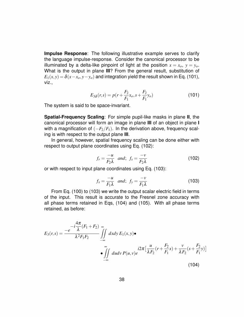
Impulse Response: The following illustrative example serves to clarifythe language impulse-response. Consider the canonical processor to beilluminated by a delta-like pinpoint of light at the position x = xo, y = yo.What is the output in plane III? From the general result, substitution ofE1(x,y)= δ (x−xo,y−yo) and integration yield the result shown in Eq. (101),viz.,

E3δ (r,s) = p(r+F2

F1xo,s+

F2

F1yo) (101)

The system is said to be space-invariant.

Spatial-Frequency Scaling: For simple pupil-like masks in plane II, thecanonical processor will form an image in plane III of an object in plane Iwith a magnification of (−F2/F1). In the derivation above, frequency scal-ing is with respect to the output plane III.

In general, however, spatial frequency scaling can be done either withrespect to output plane coordinates using Eq. (102):

fr =−uF2λ

and; fs =−vF2λ

(102)

or with respect to input plane coordinates using Eq. (103):

fx =−uF1λ

and; fy =−vF1λ

(103)

From Eq. (100) to (103) we write the output scalar electric field in termsof the input. This result is accurate to the Fresnel zone accuracy withall phase terms retained in Eqs, (104) and (105). With all phase termsretained, as before:

E3(r,s) =−e−i

4πλ

(F1 +F2)

λ 2F1F2

∞∫∫

−∞

dxdy E1(x,y)•

•∞∫∫

−∞

dudv P(u,v)ei2π[ u

λF2(r+

F2

F1x)+

vλF2

(s+F2

F1y)]

(104)

38

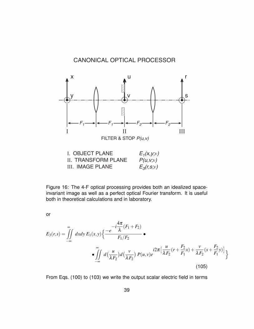
CANONICAL OPTICAL PROCESSOR

I. OBJECT PLANE E1(x,y;v)II. TRANSFORM PLANE P(u,v;v)III. IMAGE PLANE E3(r,s;v)

F1I II III

x

y

r

s

u

v

F1 F2 F2

FILTER & STOP P(u,v)

Figure 16: The 4-F optical processing provides both an idealized space-invariant image as well as a perfect optical Fourier transform. It is usefulboth in theoretical calculations and in laboratory.

or

E3(r,s) =∞∫∫

−∞

dxdy E1(x,y){−e−i

4πλ

(F1 +F2)

F1/F2•

•∞∫∫

−∞

d( u

λF2

)d( v

λF2

)P(u,v)e

i2π[ u

λF2(r+

F2

F1x)+

vλF2

(s+F2

F1y)]}

(105)

From Eqs. (100) to (103) we write the output scalar electric field in terms

39

of the input. This result is accurate to the Fresnel zone accuracy with allphase terms retained in Eqs. (104) and (105).

9 Summary

The article on Fourier optics and electromagnetic waves provides a readable,concise, and rigorous treatment that will be clear and understandable withoutparticular experience or background. There are 8 separate sections starting witha discussion of Maxwell’s equations in real-valued time dependent form. Thenin Sec. 1.2, the standard notation of the Fourier transform and its inversion isdefined. The signal representation is explained and summarized in Fig. 1.

Section 2 treats the central problem of propagation into the right-half-space.The rigorous explanation of the integral expression goes by the name Rayleigh-Sommerfeld-Smythe. The addition of the Smythe name is mine (N. George) be-cause his rigorous theory has clarified what is often confusing in the optics litera-tures. The basic equations are summarized in Eq. (33) to (36).

To make the material readable and interesting for the theorist who is not ex-perienced with Optics, we are very careful with the choice of the first illustrativeproblem. In Sec. 3.1, it is the exact calculation of the radiation along the opticalaxis [10] from a circular aperture. As an exact calculation, it serves as an ex-cellent choice for the student to really think about, There is little or no jargon aswell.

Then, in Sec. 2 the far-zone is treated using the far-zone approximation that isnot paraxially limited. Section 3.3 has the standard Fresnel zone coverage. Sec-tion 4 contains a thorough discussion of lenses from the wavefront point of view.This is Sec. 4.2. Fairly recent thinking about aspheres is presented together withan explanation of how to go from wavefront delay φ to focal length f in Eq. (90).Whenever possible the Fourier optics or wavefront presentation is made withoutparaxial approximations. It does seem that future applications with the use of dig-ital computers will greatly expand the practicality of optical system design usingFourier optics.

In the later sections of the article, we describe some important illustrations ofFourier optics. This includes the ideal F to F optical Fourier transform and thenthe 4F canonical processor. If you see errors or mistakes, my apologies, pleasesend me an email: ngeorge@optics.rochester.edu.

40

References

[1] Duffieux, P.M., The Fourier Transform and Its Applications to Optics.(English translation: Second edition) Masson, Editeur, Paris (1970)

[2] Goodman, J.W., Introduction to Fourier Optics. McGraw-Hill, NewYork, 1st Edition (1968) & 3rd Edition (2004)

[3] Papoulis, A., Systems and Transforms with Applications in Optics.McGraw-Hill, New York (1968)

[4] Griffiths, D.J., Introduction to Electrodynamics. Second Edition, Pren-tice Hall, New Jersey (1989)

[5] Papas, C.H., Theory of Electromagnetic Wave Propagation. McGraw-Hill, New York (1965)

[6] Balanis, C.A., Advanced Engineering Electromagnetics. John Wiley& Sons, New York (1989)

[7] Kong, J.A., Electromagnetic Wave Theory. EMW Publishing, Cam-bridge (2008)

[8] Smythe, W.R., Static and Dynamic Electricity. 3rd Edition, RevisedPrinting, Taylor & Francis (1989)

[9] Smythe, W.R., The Double Current Sheet in Diffraction. Phys. Rev.72, 1066 (1947)

[10] English, R.E., Jr., and George, N., Diffraction from a circular aperture:on-axis field strength. Appl. Opt. 26 (12), 2360-2363 (1987)

[11] Jackson, J.D., Classical Electrodynamics. Third Edition, John Wiley &Sons, New York (1999)

[12] Born, M., and Wolf, E. Principle of Optics. Pergamon Press, New York(1959)

[13] George, N., and Chen, X., Extended Depth-of-Field Lenses andMethods for Their Design, Optimization and Manufacturing. U.S.Patent Application Publication US2010/0002310 A1 (2010)

41

[14] Kidger, M.J., Fundamental of Optical Design. SPIE Press Monograph,PM 92 (2001)

[15] Welford, W.T., Aberrations of the Symmetrical Optical System. Aca-demic Press (1974)

[16] George, Nicholas; J.T. Thomasson, Photodetector Light Pattern De-tector. U.S. Pat. No. 3,689,772 (1972)

[17] George, Nicholas; Niels Jensen; J.T. Thomasson, Diffraction PatternSampling for Real-Time Pattern Recognition. J. Opt. Soc. Am.; 1380A(1972)

[18] Wang, Shen-ge; N. George, Fresnel zone transforms in spatially in-coherent illumination. Appl. Opt, 24, pp. 842-850 (1985)

[19] N. George; Wang, Shen-ge; and D.L. Venable, Pattern recognition us-ing the ring-wedge detector and neural network software. SPIE 1134(1989)

[20] Coston, S.D; N. George; Particle size inversion. Appl. Opt. 30, pp.4786-4794 (1991)

[21] Bertanger, D.M.; N. George, All digital ring-sedge detector applied toautomatic image quality assessment. Appl. Opt. 39, pp. 4080-4097(2000)

42

About the author

Nicholas GeorgeJoseph C. Wilson Chair Professor ofElectronic Imaging & Professor of OpticsPhone: 585-275-2417 Cell: 585-329-1029Email: ngeorge@optics.rochester.eduThe Institute of Optics, University of Rochester

Nicholas George is the Joseph C. Wilson Professor of Electronic Imaging anda Professor of Optics at the University of Rochester. He was the founding Direc-tor of the Center for Electronic Imaging Systems (CEIS), funded in part by theNational Science Foundation under the S/IUCRC program, and also of the highlyrated ARO-URI Center for Opto-Electronic Systems Research. Prior to this hewas Director of The Institute of Optics at the University of Rochester for morethan four years, serving during a period of unprecedented growth. Previously hewas a Professor of Applied Physics and Electrical Engineering at the CaliforniaInstitute of Technology. He received the B.S. degree with highest honors fromthe University of California at Berkeley, the M.S. degree in Electrical Engineer-ing from the University of Maryland, and the Ph.D. in Electrical Engineering andPhysics from the California Institute of Technology. Presently he serves as Direc-tor of the Emerging Electronic Imaging Systems Laboratory. He has served asprincipal thesis advisor to 50 doctoral students who have gone on to responsibleacademic positions, R & D systems work, and leadership positions in industryand finance. His firsts and near-firsts in modern optics include the holographicdiffraction grating, the holographic stereogram, the ring-wedge detector roboticvision system, the laser heterodyne for pollution sensing of nitrogen oxides, theinfrared hologram, the theory and experiments for the wavelength dependence ofspeckle, the FM-FM laser line scan system for remote contouring of aerial maps,and the logarithmic asphere for extended depth of field cameras.

43