Our Goal Today!

Our Goal Today!

THIS WILL NOT HAPPEN!

1

2

Final Exam Logistics ¡ Date: Friday, June 6 – Sunday, June 8

¡  Time: Any 8 hour period from 8:00AM on Friday to 8:00PM on Sunday

¡  Place: Will be available electronically

¡ Open book exam: Allow the use notes, lectures, recitations, homework

¡ ABSOLUTELY NO COLLABORATION! Violation of this will result in a failing grade for the course.

¡  Formula Sheet provided on Stellar

Outline §  Topic 1 : Probability Theory

§  Topic 2 : Decision Analysis

§  Topic 3 : Discrete Random Variables

§  Topic 4 : Continuous Random Variables

§  Topic 5 : Covariance and Correlation

§  Topic 6 : Regression

§  Topic 7 : Linear Optimization

§  Topic 8 : Discrete Optimization

§  Topic 9 : Nonlinear Optimization

3

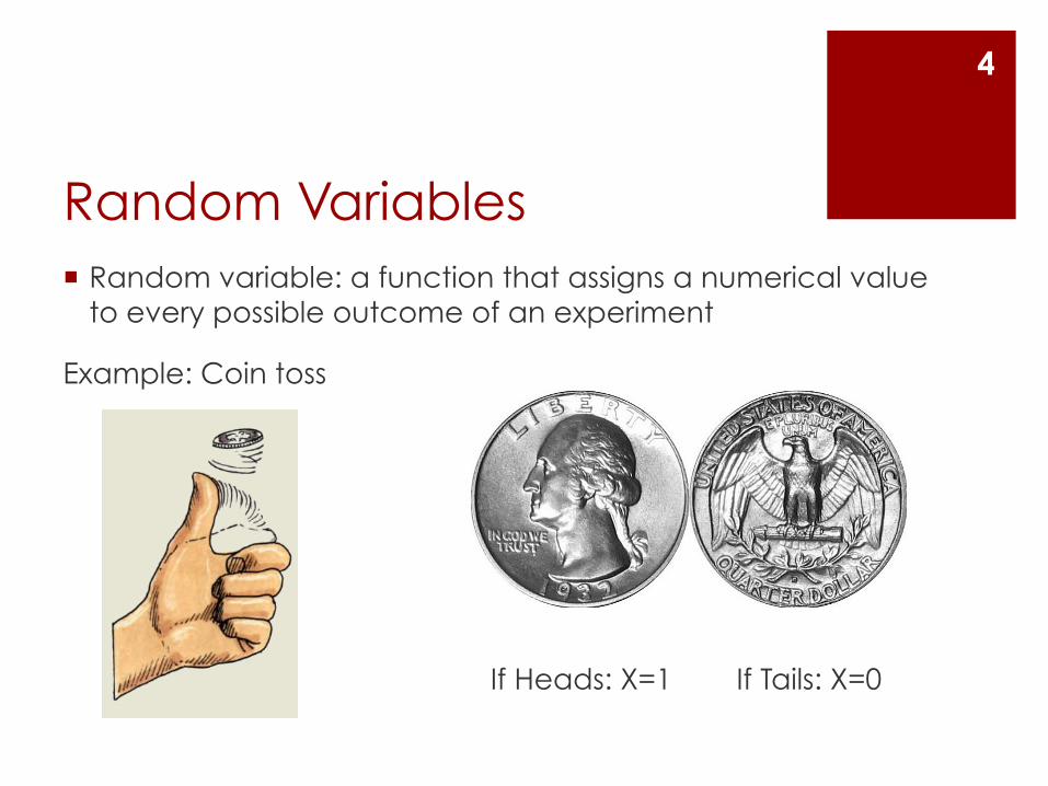
Random Variables ¡  Random variable: a function that assigns a numerical value

to every possible outcome of an experiment

Example: Coin toss

If Heads: X=1 If Tails: X=0

4

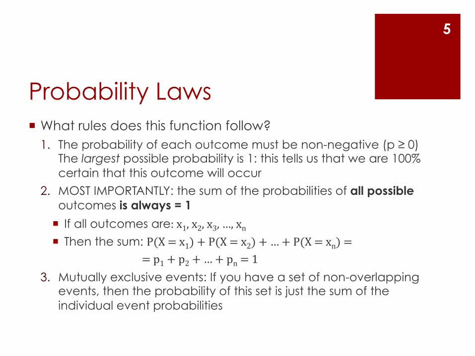
Probability Laws ¡ What rules does this function follow?

1.  The probability of each outcome must be non-negative (p ≥ 0) The largest possible probability is 1: this tells us that we are 100% certain that this outcome will occur

2.  MOST IMPORTANTLY: the sum of the probabilities of all possible outcomes is always = 1

¡  If all outcomes are: x1, x2, x3, …, xn ¡  Then the sum: P(X = x1) + P(X = x2) + … + P(X = xn) =

= p1 + p2 + … + pn = 1 3.  Mutually exclusive events: If you have a set of non-overlapping

events, then the probability of this set is just the sum of the individual event probabilities

5

¡ Mean: the “weighted” average outcome ¡  Formula:

¡ Average: the center of a set of numbers (all equally likely) ¡  Formula:

¡  THEY ARE ONLY EQUAL IF ALL PROBABILITIES pi ARE THE SAME!!

E[X]= µx = xi ⋅P(X = xi ) =i=1

n

∑ x i pii=1

n

∑

Mean (Expected Value)

6

A = 1n

xii=1

n

∑

Decision Trees Should I bring an umbrella today in case it rains?

Since 0.8 > -2, I should bring an umbrella!!! 7

Bring umbrella

Rain

Rain

Yes, p=40%

No, p=60%

Yes, p=40%

No, p=60%

Yes

No

+5

-2

0

-5

5*.4 + -2*.6 = 0.8

-5*.4 + 0*.6 = -2










8

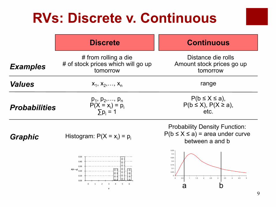
RVs: Discrete v. Continuous

9

Discrete Continuous

Examples # from rolling a die

# of stock prices which will go up tomorrow

Distance die rolls Amount stock prices go up

tomorrow

Values x1, x2,…, xn range

Probabilities p1, p2,…, pn P(X = xi) = pi ∑pi = 1

P(b ≤ X ≤ a), P(b ≤ X), P(X ≥ a),

etc.

Graphic

y

P(Y = y)

0.00

0.10

0.20

0.30

0.40

0.50

0 1 2 3 4 5 6

0

0.05

0.1

0.15

0.2

0.25

0.3

0.35

0 0.5 1 1.5 2 2.5 3 3.5 4 4.5 5

a b

Histogram: P(X = xi) = pi Probability Density Function:

P(b ≤ X ≤ a) = area under curve between a and b

RVs: Important Summary Statistics

10

Meaning Equation (Discrete)

Mean µExpected value

Variance σ2

Measure of spread around mean (units2)

Standard Deviation

σ Measure of spread around mean

(units)

∑ ∗==i

iiX xpXE µ)(

2*

2 )()( ∑ −==i

xiiX xpXVar µσ

)(XVarX =σ

Coefficient of variation

CV Unitless measure of spread

€

CVX =σXµX

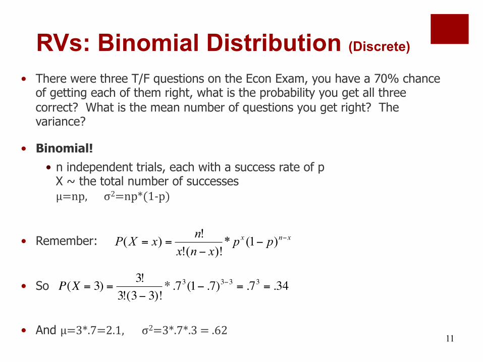
RVs: Binomial Distribution (Discrete)

•  There were three T/F questions on the Econ Exam, you have a 70% chance of getting each of them right, what is the probability you get all three correct? What is the mean number of questions you get right? The variance?

•  Binomial! •  n independent trials, each with a success rate of p

X ~ the total number of successes µμ=np, σ2=np*(1-‐p)

•  Remember:

•  So

•  And µμ=3*.7=2.1, σ2=3*.7*.3 = .62

11

xnx ppxnx

nxXP −−

−== )1(*

)!(!!)(

€

P(X = 3) =3!

3!(3− 3)!* .73(1− .7)3−3 = .73 = .34

12

0

0.02

0.04

0.06

0.08

0.1

0.12

-6 -4 -2 0 2 4 6 8 10 12

Computing probabilities with the Normal distribution:

You want : P(a ≤ X ≤ b) where X is N(µ,σ)

1. Define : : Z is N(0,1)

2. Use the standard normal probability table (Z table)

σµ−

=XZ

)()(

)()(

σµ

σµ

σµ

σµ

−≤−

−≤=

−≤≤

−=≤≤

aZPbZP

bZaPbXaP

Bell-shaped curve

RVs: Normal Distribution (Continuous)

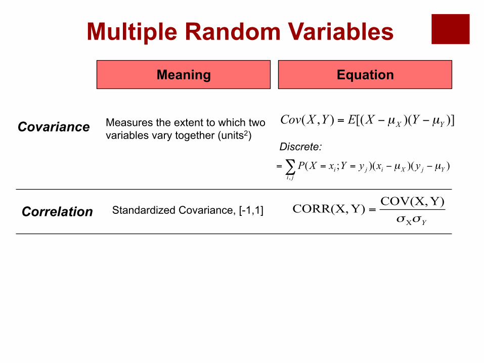
Multiple Random Variables Meaning Equation

Covariance Measures the extent to which two variables vary together (units2)

Correlation Standardized Covariance, [-1,1]

)])([(),( YX YXEYXCov µµ −−=

YσσX

Y)COV(X,Y)CORR(X, =

∑ −−===ji

YjXiji yxyYxXP,

))()(;( µµ

Discrete:

14

d)  If X has mean 1, standard deviation 2 and Y has mean 1, standard deviation 4, then the standard deviation of Z=X+Y cannot exceed 6.

Var(Z) = Var(X) + Var(Y) + 2*σX*σY*CORR(X,Y) Maximum value achieved when CORR(X,Y) = 1

Var(Z) = 36, σZ = 6

2005 Exam: Problem 1 (d)

nn XXXS +++= ...21• For n>30, is approximately normal with mean n.µ and variance n.σ2 (standard deviation √n.σ)

nXXXM n

n+++

=...21

• For n>30, is approximately normal with mean µ and variance σ2/n (standard deviation σ/√n )

15

X1, X2, ..., Xn independent identically distributed random variables: E[Xi] = µ, Var(Xi) = σ2

• The probability distribution of Xi does not matter; •  n does not have to be very large (30 is good enough); •  CLT requires only 2 pieces of information: the mean and SD of Xi

Sums of i.i.d RVs: Central Limit Theorem

Silverware Example

16

•  SilverwareInc has 3 products: Forks, Knives, and Spoons. They have kept track of sales, but only in aggregate form. They have found that the mean of yearly Silverware revenues is $3M, and the standard deviation of the yearly revenues is $1M. Revenues are Normally Distributed

•  What can you say about the distribution of the yearly revenues?

• W = F+K+S ~ N(µ=3, σ=1), in $M

Silverware Example

17

•  SilverwareInc is selling world-class Forks, Knives, and Spoons. The mean and standard deviation of the number of daily sets sold are recorded in the table below, together with the price.

•  What can you say about the distribution of yearly sales of forks? •  F ~ N(µ=365*15.6, σ=8.3*√365)

Forks Knives Spoons

Mean 15.6 17.2 22.4

St Dev 8.3 7.2 8.5

Price ($) 10.0 10.0 11.0

•  What can you say about the distribution of yearly sales of forks? •  F ~ N(µ=365*15.6, σ=8.3*√365)

• What is the probability that SilverwareInc’s revenues from forks is greater than 6,000 units this year?

Silverware Example

€

P(W >= 6000) = P(W −µσ

>=6000 −µ

σ)

= P(Z >=6000 − 5694158.57

) = P(Z >=1.92)

=1− P(Z <=1.92)










19

Linear Regression

•  Predict a dependent variable Y from a set of independent variables (predictors) Xi

•  Assume Y is a “straight-line” function of each of the Xi variables, when all the others are fixed.

•  The slopes of each Xi’s relationship with Y are coefficients βi

•  Goal: Pick coefficients to minimize errors (sum of squared residuals) ŷi = b0 + b1x1i + . . . + bkxki

•  The steps in which we accomplish this goal are as follows:

•  Calculate the model parameters that “best agree” with the available data (βk).

•  Analyze the model and estimates and verify that they are reasonable.

•  Potentially revise initial model based on this analysis, and repeat.

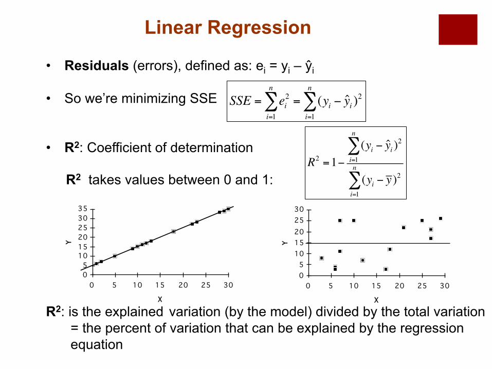
•  Residuals (errors), defined as: ei = yi – ŷi

•  So we’re minimizing SSE

•  R2: Coefficient of determination

R2: is the explained variation (by the model) divided by the total variation

= the percent of variation that can be explained by the regression equation

Linear Regression

SSE = ei2

i=1

n

∑ = (yi − yi )2

i=1

n

∑

R2 =1−(yi − yi )

2

i=1

n

∑

(yi − y )2

i=1

n

∑ R2 takes values between 0 and 1:

X

Y

05

101520253035

0 5 10 15 20 25 30

X

Y05

1015202530

0 5 10 15 20 25 30

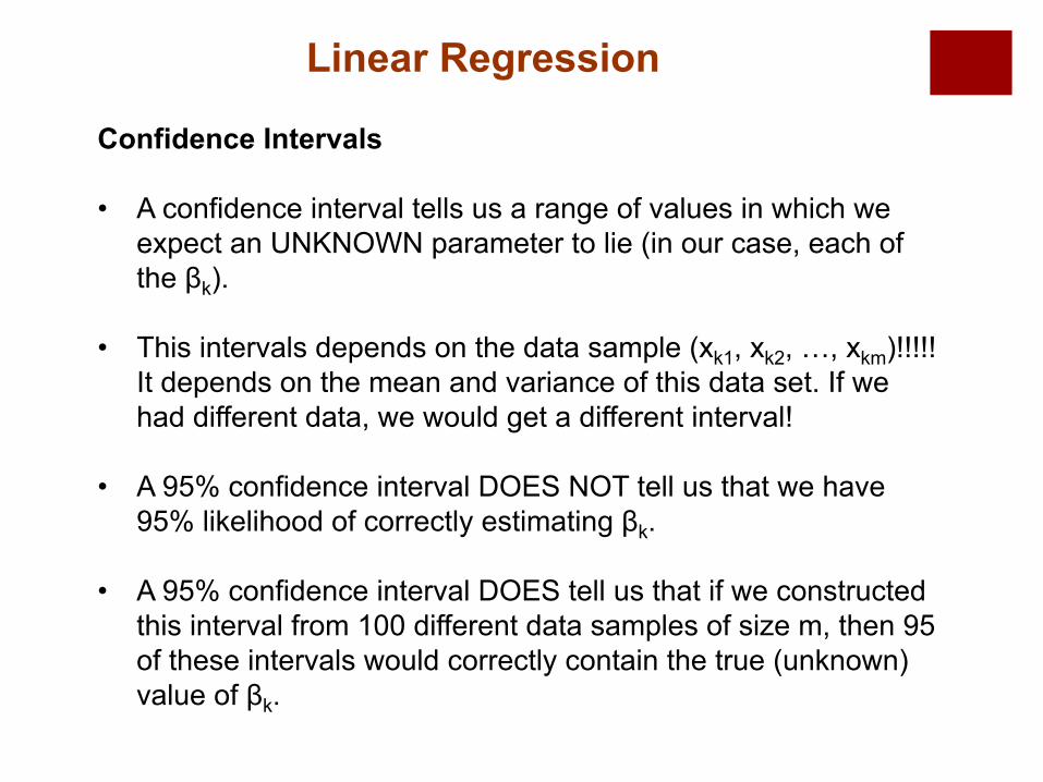
Confidence Intervals •  A confidence interval tells us a range of values in which we

expect an UNKNOWN parameter to lie (in our case, each of the βk).

•  This intervals depends on the data sample (xk1, xk2, …, xkm)!!!!! It depends on the mean and variance of this data set. If we had different data, we would get a different interval!

•  A 95% confidence interval DOES NOT tell us that we have 95% likelihood of correctly estimating βk.

•  A 95% confidence interval DOES tell us that if we constructed

this interval from 100 different data samples of size m, then 95 of these intervals would correctly contain the true (unknown) value of βk.

Linear Regression

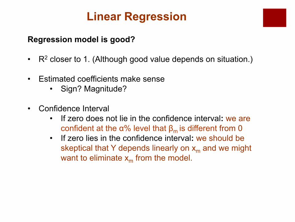
Regression model is good? •  R2 closer to 1. (Although good value depends on situation.)

•  Estimated coefficients make sense •  Sign? Magnitude?

•  Confidence Interval

•  If zero does not lie in the confidence interval: we are confident at the α% level that βm is different from 0

•  If zero lies in the confidence interval: we should be skeptical that Y depends linearly on xm and we might want to eliminate xm from the model.

Linear Regression

•  Multicollinearity: Are two explanatory variables correlated? Signs: if regression coeffs have “wrong” sign or we find high R2 but one or more of the regression coeffs is not significantly different from 0. Check correlation table. Remove one of the variables from the model if there is high correlation.

Checklist for Evaluating a Linear Regression Model

•  Linearity: Construct a scatter-plot for each explanatory variable check for linearity.

•  Signs of Regression Coefficients: Check to see that the signs make intuitive sense.

•  Significance tests: check if the regression coefficients are significantly different from zero (not included in the confidence interval).

•  R2: Check if the value of R2 is reasonably high.

•  Normality: Check that the residuals are approximately Normally distributed by constructing a histogram of residuals.

•  Heteroscedasticity: Do error terms have constant standard deviation? Plot the residuals with the observed values of each of the explanatory variables.

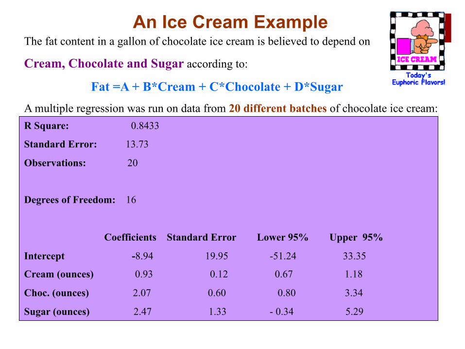
An Ice Cream Example The fat content in a gallon of chocolate ice cream is believed to depend on

Cream, Chocolate and Sugar according to:

Fat =A + B*Cream + C*Chocolate + D*Sugar A multiple regression was run on data from 20 different batches of chocolate ice cream: R Square: 0.8433

Standard Error: 13.73

Observations: 20

Degrees of Freedom: 16

Coefficients Standard Error Lower 95% Upper 95%

Intercept -8.94 19.95 -51.24 33.35

Cream (ounces) 0.93 0.12 0.67 1.18

Choc. (ounces) 2.07 0.60 0.80 3.34

Sugar (ounces) 2.47 1.33 - 0.34 5.29

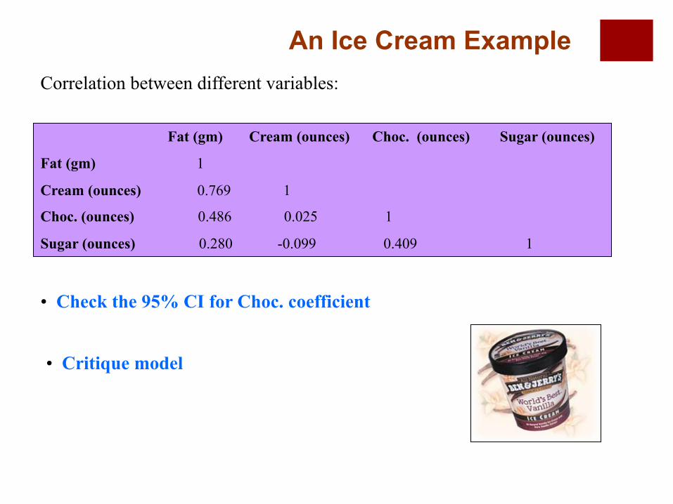
Fat (gm) Cream (ounces) Choc. (ounces) Sugar (ounces)

Fat (gm) 1

Cream (ounces) 0.769 1

Choc. (ounces) 0.486 0.025 1

Sugar (ounces) 0.280 -0.099 0.409 1

Correlation between different variables:

•  Check the 95% CI for Choc. coefficient

•  Critique model

An Ice Cream Example

Signs of Regression Coefficients Coefficients Standard Error Lower 95% Upper 95%

Intercept -8.94 19.95 -51.24 33.35

Cream (ounces) 0.93 0.12 0.67 1.18

Choc. (ounces) 2.07 0.60 0.80 3.34

Sugar (ounces) 2.47 1.33 - 0.34 5.29

The coefficients for Cream, Choc and Sugar appear to make sense.

•  Critique model

Significance test: 0 is in the confidence interval for Sugar coeff. so Sugar should be excluded from the regression.


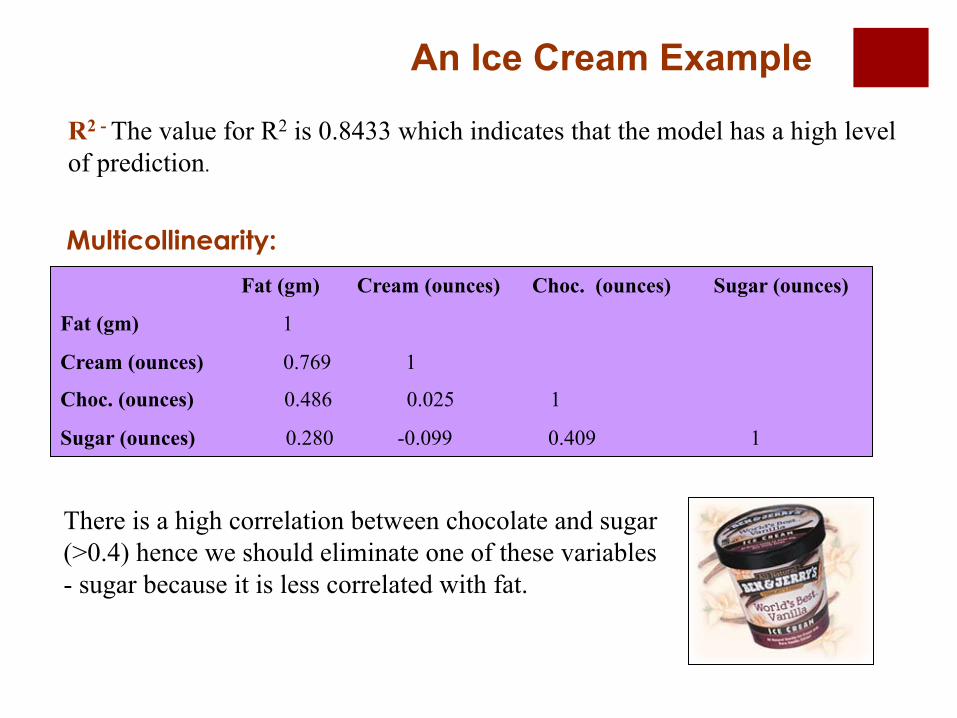
R2 - The value for R2 is 0.8433 which indicates that the model has a high level of prediction.

Multicollinearity:

Fat (gm) Cream (ounces) Choc. (ounces) Sugar (ounces)

Fat (gm) 1

Cream (ounces) 0.769 1

Choc. (ounces) 0.486 0.025 1

Sugar (ounces) 0.280 -0.099 0.409 1

There is a high correlation between chocolate and sugar (>0.4) hence we should eliminate one of these variables - sugar because it is less correlated with fat.


There appears to be no heteroscedasticity

Heteroscedasticity:

Res

idua

ls

Chocolate (ounces)

0

Chocolate Residual Plot

Res

idua

ls

Cream (ounces)

0

Cream Residual Plot


The residuals appear to be normally distributed

Residual

Freq

uenc

y

Residual Frequency

Residual Distribution:











31

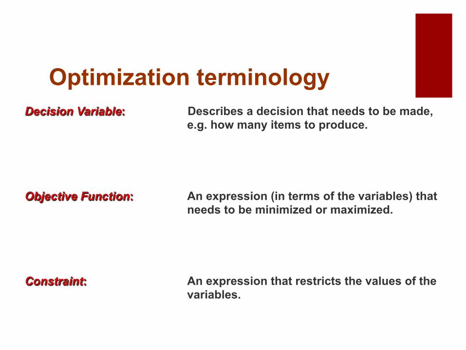
Decision Variable: Describes a decision that needs to be made, e.g. how many items to produce.

Objective Function: An expression (in terms of the variables) that needs to be minimized or maximized.

Constraint: An expression that restricts the values of the variables.

Optimization terminology

Steps in formulation

1. Define the decision variables.

2. Write the objective as a function of these vars. Determine whether max or min.

3. Write the constraints as functions of these vars. Either ≤ , ≥ , = .

4. Determine the variable restrictions, e.g. non-negative, integer. Be careful of units!

�  Associated with each constraint.

�  Shadow price = 0 for non-binding constraints.

�  The shadow price is the change in the objective value per unit change in the right hand side, given all other data remain the same.

�  Allowable range (decrease/increase)

�  If r.h.s changes within range: Shadow price tells us rate of change in the optimal objective function value; we know exactly the new objective value without re-solving the problem.

�  If r.h.s changes outside range: We cannot determine the rate of change in the optimal objective value anymore; we need to solve the optimization pb again!

About Shadow Prices

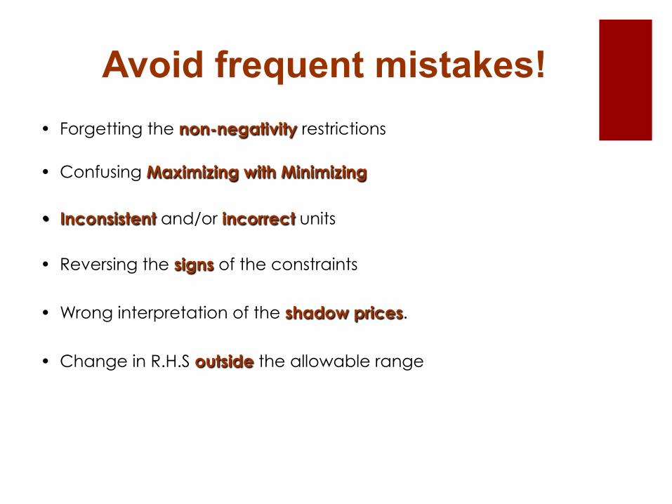
•  Forgetting the non-negativity restrictions

•  Confusing Maximizing with Minimizing

•  Inconsistent and/or incorrect units

•  Reversing the signs of the constraints

•  Wrong interpretation of the shadow prices.

•  Change in R.H.S outside the allowable range

Avoid frequent mistakes!

2007 Exam – Problem 3 Sloan Alloy Corp. manufactures four different types of alloys for aircraft construction, denoted A, B, C and D, from three basic metals: aluminum, copper and magnesium. The profit margins for each of the alloys are $105, $45, $95, and $140 per ton, for alloys A, B, C, and D, respectively. The proportion of metals in the alloys is shown in the following table.

A B C D Aluminum 0.3 0.4 0.1 0.15 Copper 0.3 0.1 0.25 0.4 Magnesium 0.4 0.5 0.65 0.45

For example, one ton of alloy A consists of 0.3 tons of aluminum, 0.3 tons of copper and 0.4 tons of magnesium. The monthly maximum supplies of aluminum, copper and magnesium are 600, 400 and 800 tons per month, respectively.

2007 Exam – Problem 3

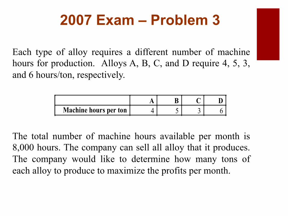
Each type of alloy requires a different number of machine hours for production. Alloys A, B, C, and D require 4, 5, 3, and 6 hours/ton, respectively.

The total number of machine hours available per month is 8,000 hours. The company can sell all alloy that it produces. The company would like to determine how many tons of each alloy to produce to maximize the profits per month.

A B C D Machine hours per ton 4 5 3 6

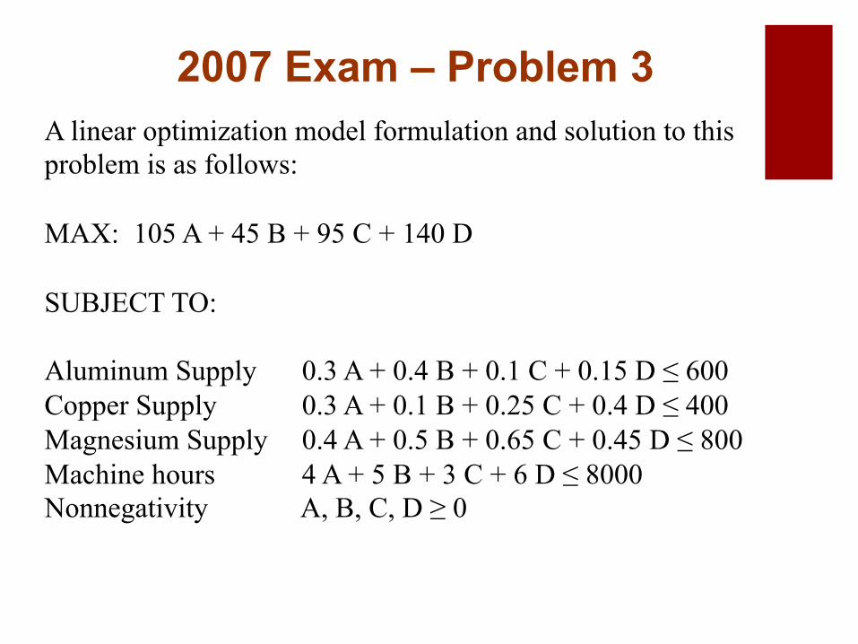
2007 Exam – Problem 3 A linear optimization model formulation and solution to this problem is as follows: MAX: 105 A + 45 B + 95 C + 140 D SUBJECT TO: Aluminum Supply 0.3 A + 0.4 B + 0.1 C + 0.15 D ≤ 600 Copper Supply 0.3 A + 0.1 B + 0.25 C + 0.4 D ≤ 400 Magnesium Supply 0.4 A + 0.5 B + 0.65 C + 0.45 D ≤ 800 Machine hours 4 A + 5 B + 3 C + 6 D ≤ 8000 Nonnegativity A, B, C, D ≥ 0

2007 Exam – Problem 3 (a) Adjustable Cells Final Reduced Objective Allowable Allowable Cell Name Value Cost Coefficient Increase Decrease $B$10 A 0 -1.1 105 1.1 1E+30 $C$10 B 632.4 0.0 45 12.5 2.1 $D$10 C 284.6 0.0 95 2.0 4.2 $E$10 D 664.0 0.0 140 14.2 1.8 Constraints Final Shadow Constraint Allowable Allowable Cell Name Value Price R.H. Side Increase Decrease $B$16 Aluminum Supply 381.03 0 600 1E+30 219.0 $B$17 Copper Supply 400 318.6 400 156.9 202.9 $B$18 Magnesium Supply 800 21.3 800 442.1 128.6 $B$19 Machine Time 8000 0.5 8000 1161.3 2711.9

(a) (4 points) What is the optimal solution? What is the optimal profit per month? Optimal solution: 0 tons of A, 632.4 of B, 284.6 of C and 664 of D. Optimal profit: 105 * 0 + 45 * 632.4 + 95 * 284.6 + 140 * 664 = $148,455/mth

2007 Exam – Problem 3 (b)

(b) (2 points) Which are the binding constraints? Binding constraints: Supply of copper and magnesium and the available machine time.

Adjustable Cells Final Reduced Objective Allowable Allowable Cell Name Value Cost Coefficient Increase Decrease $B$10 A 0 -1.1 105 1.1 1E+30 $C$10 B 632.4 0.0 45 12.5 2.1 $D$10 C 284.6 0.0 95 2.0 4.2 $E$10 D 664.0 0.0 140 14.2 1.8 Constraints Final Shadow Constraint Allowable Allowable Cell Name Value Price R.H. Side Increase Decrease $B$16 Aluminum Supply 381.03 0 600 1E+30 219.0 $B$17 Copper Supply 400 318.6 400 156.9 202.9 $B$18 Magnesium Supply 800 21.3 800 442.1 128.6 $B$19 Machine Time 8000 0.5 8000 1161.3 2711.9

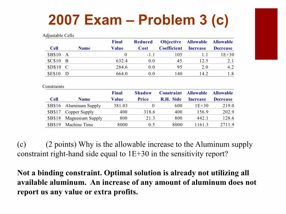
2007 Exam – Problem 3 (c)

(c) (2 points) Why is the allowable increase to the Aluminum supply constraint right-hand side equal to 1E+30 in the sensitivity report? Not a binding constraint. Optimal solution is already not utilizing all available aluminum. An increase of any amount of aluminum does not report us any value or extra profits.


2007 Exam – Problem 3 (d)

(d) (3 points) Assuming all other data are unchanged, what would the new optimal profit be, if we realize we have to perform preventive maintenance to the machines, which will decrease the available machine hours per month by 200 hours? Our profits will decrease by 0.5 * 200 = $100 / month.


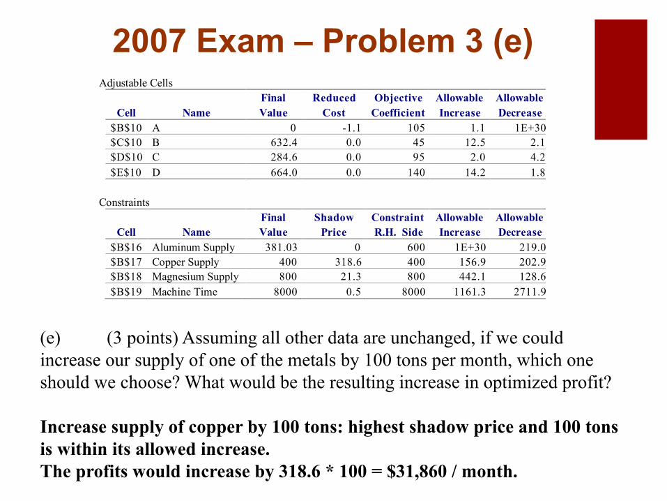
2007 Exam – Problem 3 (e)

(e) (3 points) Assuming all other data are unchanged, if we could increase our supply of one of the metals by 100 tons per month, which one should we choose? What would be the resulting increase in optimized profit? Increase supply of copper by 100 tons: highest shadow price and 100 tons is within its allowed increase. The profits would increase by 318.6 * 100 = $31,860 / month.


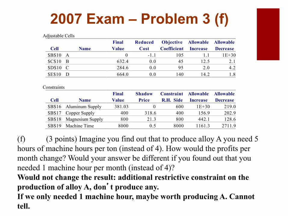
2007 Exam – Problem 3 (f)

(f) (3 points) Imagine you find out that to produce alloy A you need 5 hours of machine hours per ton (instead of 4). How would the profits per month change? Would your answer be different if you found out that you needed 1 machine hour per month (instead of 4)? Would not change the result: additional restrictive constraint on the production of alloy A, don’t produce any. If we only needed 1 machine hour, maybe worth producing A. Cannot tell.


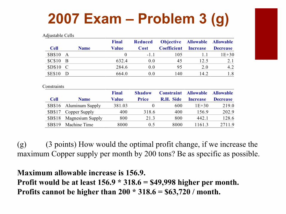
2007 Exam – Problem 3 (g)

(g) (3 points) How would the optimal profit change, if we increase the maximum Copper supply per month by 200 tons? Be as specific as possible. Maximum allowable increase is 156.9. Profit would be at least 156.9 * 318.6 = $49,998 higher per month. Profits cannot be higher than 200 * 318.6 = $63,720 / month.











46

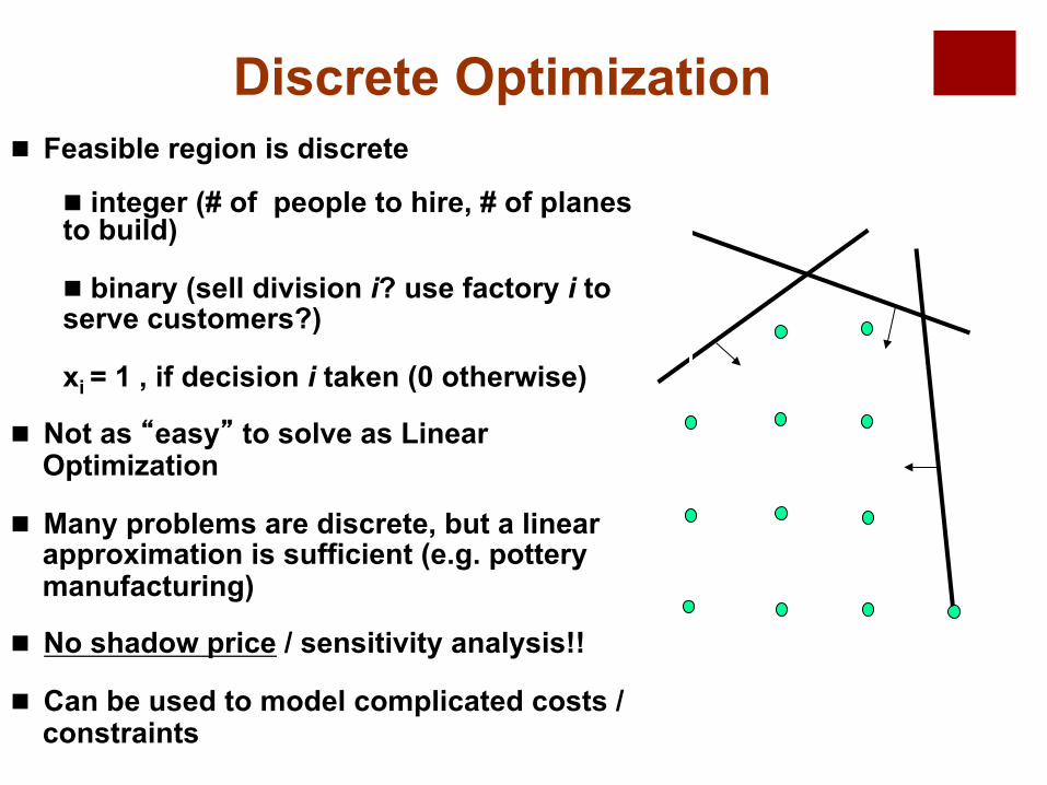
Discrete Optimization

x1

x2

0

1

2

3

4

0 1 2

3

n  Feasible region is discrete

n  integer (# of people to hire, # of planes to build)

n  binary (sell division i? use factory i to serve customers?)

xi = 1 , if decision i taken (0 otherwise)

n  Not as “easy” to solve as Linear Optimization

n  Many problems are discrete, but a linear approximation is sufficient (e.g. pottery manufacturing)

n  No shadow price / sensitivity analysis!!

n  Can be used to model complicated costs / constraints

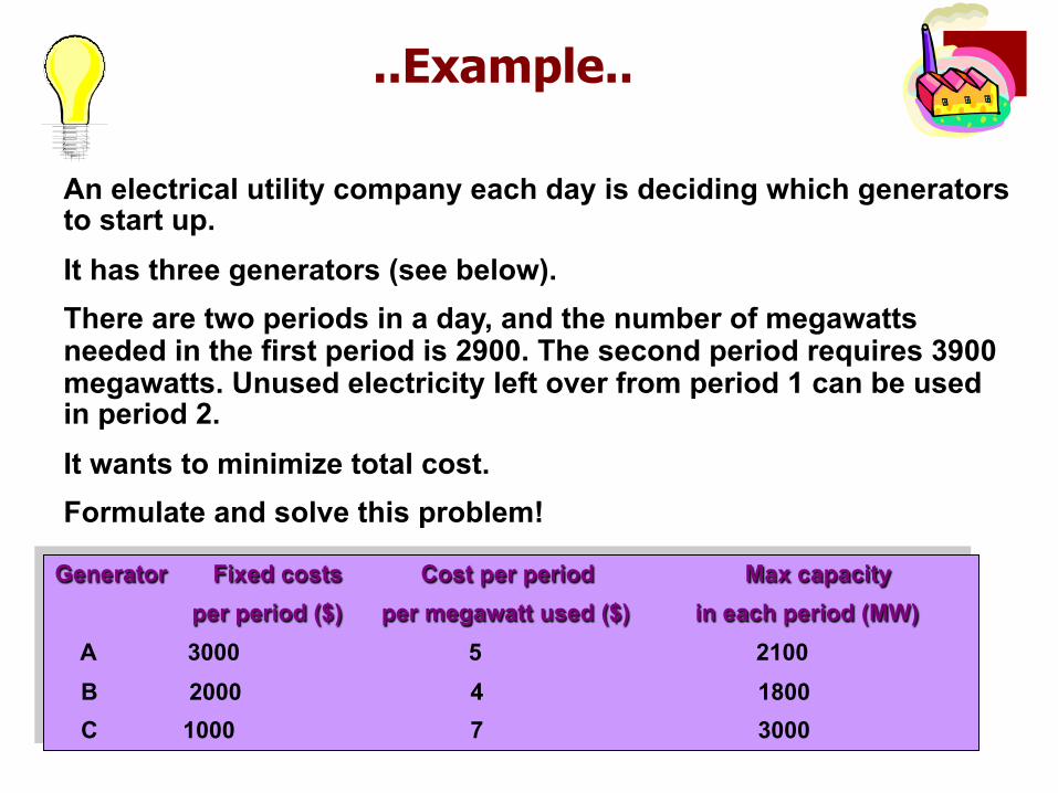
..Example..

An electrical utility company each day is deciding which generators to start up. It has three generators (see below). There are two periods in a day, and the number of megawatts needed in the first period is 2900. The second period requires 3900 megawatts. Unused electricity left over from period 1 can be used in period 2. It wants to minimize total cost. Formulate and solve this problem!

Generator Fixed costs Cost per period Max capacity per period ($) per megawatt used ($) in each period (MW) A 3000 5 2100 B 2000 4 1800 C 1000 7 3000

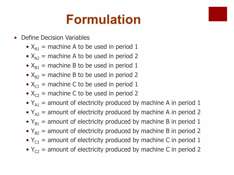
•  Define Decision Variables •  XA1 = machine A to be used in period 1 •  XA2 = machine A to be used in period 2 •  XB1 = machine B to be used in period 1 •  XB2 = machine B to be used in period 2 •  XC1 = machine C to be used in period 1 •  XC2 = machine C to be used in period 2 •  YA1 = amount of electricity produced by machine A in period 1 •  YA2 = amount of electricity produced by machine A in period 2 •  YB1 = amount of electricity produced by machine B in period 1 •  YB2 = amount of electricity produced by machine B in period 2 •  YC1 = amount of electricity produced by machine C in period 1 •  YC2 = amount of electricity produced by machine C in period 2

Formulation

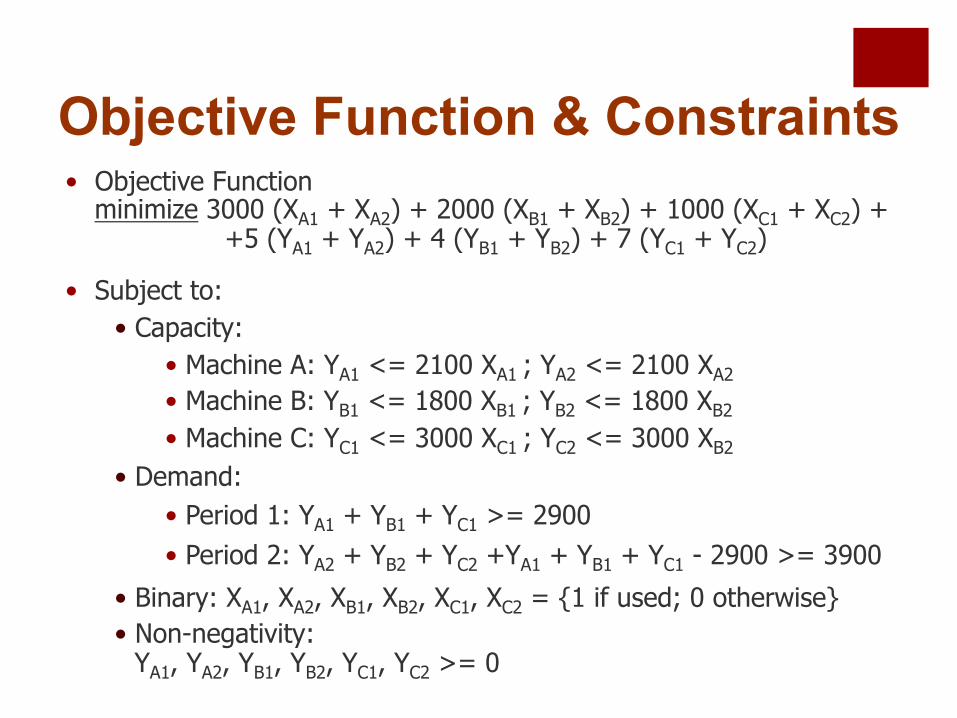
•  Objective Function minimize 3000 (XA1 + XA2) + 2000 (XB1 + XB2) + 1000 (XC1 + XC2) +

+5 (YA1 + YA2) + 4 (YB1 + YB2) + 7 (YC1 + YC2)

•  Subject to: • Capacity:

• Machine A: YA1 <= 2100 XA1 ; YA2 <= 2100 XA2 • Machine B: YB1 <= 1800 XB1 ; YB2 <= 1800 XB2 • Machine C: YC1 <= 3000 XC1 ; YC2 <= 3000 XB2

• Demand: •  Period 1: YA1 + YB1 + YC1 >= 2900 •  Period 2: YA2 + YB2 + YC2 +YA1 + YB1 + YC1 - 2900 >= 3900

• Binary: XA1, XA2, XB1, XB2, XC1, XC2 = {1 if used; 0 otherwise} • Non-negativity:

YA1, YA2, YB1, YB2, YC1, YC2 >= 0

Objective Function & Constraints

Excel Solution

Fixed + Variable = Total10000 30400 40400

Cost:A B C

3000 2000 10005 4 7

Decision Variables and Constraints:

Xij (0 or 1) Yij Limit * Xij Limit DemandA 1 2100 <= 2100 2100B 1 1800 <= 1800 1800C 0 0 <= 0 3000A 1 1100 <= 2100 2100B 1 1800 <= 1800 1800C 0 0 <= 0 3000

Xij binaryXij, Yij >= 0

Total

Cost per megawatt Fixed Cost per period

Objective Function:

Per

iod

1

>= 3900

>= 2900

= 3900

3900

Other constraints:

2900 + 1000

Per

iod

2

52

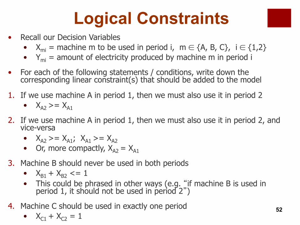
•  Recall our Decision Variables •  Xmi = machine m to be used in period i, m ∈ {A, B, C}, i ∈ {1,2} •  Ymi = amount of electricity produced by machine m in period i

•  For each of the following statements / conditions, write down the corresponding linear constraint(s) that should be added to the model

1.  If we use machine A in period 1, then we must also use it in period 2 •  XA2 >= XA1

2.  If we use machine A in period 1, then we must also use it in period 2, and vice-versa •  XA2 >= XA1; XA1 >= XA2 •  Or, more compactly, XA2 = XA1

3.  Machine B should never be used in both periods •  XB1 + XB2 <= 1

•  This could be phrased in other ways (e.g. “if machine B is used in period 1, it should not be used in period 2”)

4.  Machine C should be used in exactly one period •  XC1 + XC2 = 1

Logical Constraints

53

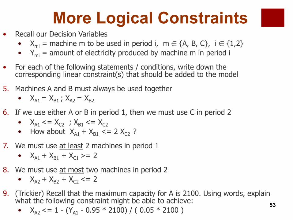
•  Recall our Decision Variables •  Xmi = machine m to be used in period i, m ∈ {A, B, C}, i ∈ {1,2} •  Ymi = amount of electricity produced by machine m in period i

•  For each of the following statements / conditions, write down the corresponding linear constraint(s) that should be added to the model

5.  Machines A and B must always be used together •  XA1 = XB1 ; XA2 = XB2

6.  If we use either A or B in period 1, then we must use C in period 2 •  XA1 <= XC2 ; XB1 <= XC2 •  How about XA1 + XB1 <= 2 XC2 ?

7.  We must use at least 2 machines in period 1 •  XA1 + XB1 + XC1 >= 2

8.  We must use at most two machines in period 2 •  XA2 + XB2 + XC2 <= 2

9.  (Trickier) Recall that the maximum capacity for A is 2100. Using words, explain what the following constraint might be able to achieve: •  XA2 <= 1 - (YA1 - 0.95 * 2100) / ( 0.05 * 2100 )

More Logical Constraints










54

Steps in a Formulation

0. Same steps as LP, but objective and constraints can be non-linear (eg. Minimize x2+y2; x*y+y<=5)

1. Define the decision variables.

2. Write the objective as a function of these vars. Determine whether max or min.

3.  Write the constraints as functions of these vars. Either ≤ , ≥ , =.

4. Determine the variable restrictions,

e.g. non-negative, integer. Be careful of units!

Example of a Sensitivity Report

All Lagrange Multipliers are zero!

All constraints are non-binding around the close proximity of the optimal solution.

Optimal solution occurs in the interior of the feasible region.

Microsoft Excel 10.0 Sensitivity ReportWorksheet: [Book1]ProductsReport Created: 12/9/2004 10:19:06 PM

Adjustable CellsFinal Reduced

Cell Name Value Gradient$B$8 units 58.82 0$C$8 units 23.53 0$D$8 units 125.00 0$B$9 units 58.82 0$C$9 units 23.53 0$D$9 units 125.00 0

ConstraintsFinal Lagrange

Cell Name Value Multiplier$B$19 machine 1 capacity LHS 578.68 0$B$20 machine 2 capacity LHS 180.59 0$B$21 product A limit LHS 117.65 0$B$22 product B limit LHS 47.06 0$B$23 product C limit LHS 250.00 0$B$11 Price A units 105.88$ -$ $B$12 Price B units 35.29$ -$ $B$13 Price C units 250.00$ -$

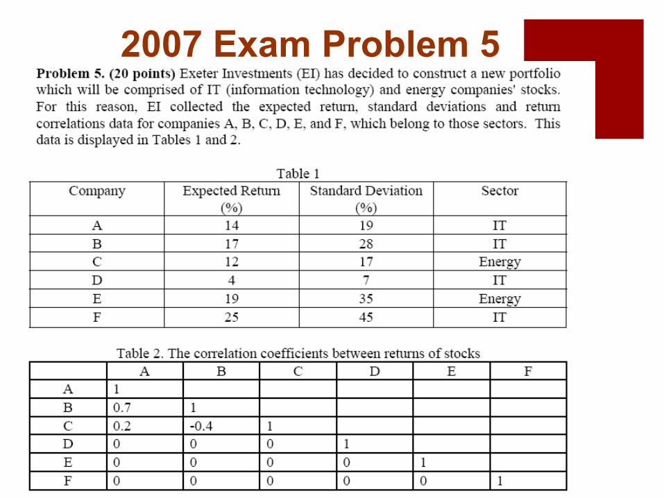
2007 Exam Problem 5

2007 Exam Problem 5

Decision Variables: wi—what percentage of the portfolio do I invest in stock i for i=A,B…F

) weightsnegative-Non(0,,,,,)portfolio leInvest who(1

)maximumRisk (1517192.0217284.0228197.02

45357172819

)return Portfolio(25194121714max

222222222222

≥

=+++++

≤⋅⋅⋅⋅+⋅⋅⋅⋅−⋅⋅⋅⋅+

+++++

+++++

FEDCBA

FEDCBA

CACBBA

FEDCBA

FEDCBA

wwwwwwwwwwww

wwwwwwwwwwww

wwwwww

+:Raising the risk maximum makes the feasible region bigger (we are less restricted). Since we are maximizing, this means we may find a new optimum with a higher return. Thus the shadow price is >=0.

2007 Exam Problem 5

A, B, D, F are IT companies. We add the constraint:

1728197.024572819 22222222 ≤⋅⋅⋅⋅++++ BAFDBA wwwwww

C and E are Energy companies. We add the constraints:

1408.01008.0 ≤+≤ EC ww

(d) (5 points) As of December 10 close, the market capitalization of energy stocks represented 12.08% of the overall S&P 500 market capitalization. EI would like to make sure that in their portfolio, the relative value of energy stocks is within +/- 2% of this S&P 500 benchmark. Show how EI can incorporate this requirement into their formulation.

(c) (4 points) Additionally EI wants to ensure that the risk corresponding to the part of the portfolio consisting of EI companies does not exceed 17%. Incorporate this requirement into your formulation.

Office Hour today at 4:15PM in the same room (E62-262)!

60

Our Goal Today!

Documents

Transcript of Our Goal Today!