Organochlorine Pesicides and PCB's in Stream Sediment and ... · U.S. GEOLOGICAL SURVEY...
95
U.S. GEOLOGICAL SURVEY Water-Resources Investigations Report Organochlorine Pesticides and PCBs in Stream Sediment and Aquatic Biota—Initial Results from the National Water-Quality Assessment Program, 1992–1995 By Charles S. Wong, 1 Paul D. Capel, 2 and Lisa H. Nowell 2 Sacramento, California 2000 00-4053 8056-67 1 University of Minnesota (present affiliation: University of Toronto) 2 U.S. Geological Survey
-
Upload
truongngoc -
Category
Documents
-
view
216 -
download
0
Transcript of Organochlorine Pesicides and PCB's in Stream Sediment and ... · U.S. GEOLOGICAL SURVEY...

U.S. GEOLOGICAL SURVEY
Water-Resources Investigations Report
Organochlorine Pesticides and PCBs in Stream Sediment and Aquatic Biota—Initial Results from the National Water-Quality Assessment Program, 1992–1995
By
Charles S. Wong,
1
Paul D. Capel,
2
and
Lisa H. Nowell
2
Sacramento, California2000
00-4053
8056
-67
1
University of Minnesota (present affiliation: University of Toronto)
2
U.S. Geological Survey

U.S. DEPARTMENT OF THE INTERIORBRUCE BABBITT, Secretary
U.S. GEOLOGICAL SURVEY
Charles G. Groat, Director
The use of firm, trade, and brand names in this report is for identification purposes only and doesnot constitute endorsement by the U.S. Geological Survey
For additional information write to: Copies of this report can be purchased
U.S. Geological SurveyBranch of Information ServicesBox 25286Denver, CO 80225-0286
from:
District ChiefU.S. Geological SurveyWater Resources DivisionPlacer Hall 6000 J StreetSacramento, California 95819-6129

Robert M. HirschAssociate Director for Water
FOREWORD
The U.S. Geological Survey (USGS) is committed to
serve the Nation with accurate and timely scientific infor-
mation that helps enhance and protect the overall quality of
life, and facilitates effective management of water, biologi-
cal, energy, and mineral resources. (http://www.usgs.gov/).
Information on the quality of the Nation’s water resources is
of critical interest to the USGS because it is so integrally
linked to the long-term availability of water that is clean and
safe for drinking and recreation and that is suitable for
industry, irrigation, and habitat for fish and wildlife. Esca-
lating population growth and increasing demands for the
multiple water uses make water availability, now measured
in terms of quantity and quality, even more critical to the
long-term sustainability of our communities and ecosys-
tems.
The USGS implemented the National Water-Quality
Assessment (NAWQA) Program to support national,
regional, and local information needs and decisions related
to water-quality management and policy. (http://
water.usgs.gov/nawqa). Shaped by and coordinated with
ongoing efforts of other Federal, State, and local agencies,
the NAWQA Program is designed to answer: What is the
condition of our Nation’s streams and ground water? How
are the conditions changing over time? How do natural fea-
tures and human activities affect the quality of streams and
ground water, and where are those effects most pro-
nounced? By combining information on water chemistry,
physical characteristics, stream habitat, and aquatic life, the
NAWQA Program aims to provide science-based insights
for current and emerging water issues and priorities.
NAWQA results can contribute to informed decisions that
result in practical and effective water-resource management
and strategies that protect and restore water quality.
Since 1991, the NAWQA Program has implemented
interdisciplinary assessments in more than 50 of the
Nation’s most important river basins and aquifers, referred
to as Study Units. (http://water.usgs.gov/nawqa/
nawqamap.html). Collectively, these Study Units account
for more than 60 percent of the overall water use and popu-
lation served by public water supply, and are representative
of the Nation’s major hydrologic landscapes, priority eco-
logical resources, and agricultural, urban, and natural
sources of contamination.
Each assessment is guided by a nationally consistent
study design and methods of sampling and analysis. The
assessments thereby build local knowledge about water-
quality issues and trends in a particular stream or aquifer
while providing an understanding of how and why water
quality varies regionally and nationally. The consistent,
multi-scale approach helps to determine if certain types of
water-quality issues are isolated or pervasive, and allows
direct comparisons of how human activities and natural pro-
cesses affect water quality and ecological health in the
Nation’s diverse geographic and environmental settings.
Comprehensive assessments on pesticides, nutrients, vola-
tile organic compounds, trace metals, and aquatic ecology
are developed at the national scale through comparative
analysis of the Study-Unit findings. (http://water.usgs.gov/
nawqa/natsyn.html).
The USGS places high value on the communication
and dissemination of credible, timely, and relevant science
so that the most recent and available knowledge about water
resources can be applied in management and policy deci-
sions. We hope this NAWQA publication will provide you
the needed insights and information to meet your needs, and
thereby foster increased awareness and involvement in the
protection and restoration of our Nation’s waters.
The NAWQA Program recognizes that a national
assessment by a single program cannot address all water-
resource issues of interest. External coordination at all lev-
els is critical for a fully integrated understanding of water-
sheds and for cost-effective management, regulation, and
conservation of our Nation’s water resources. The Program,
therefore, depends extensively on the advice, cooperation,
and information from other Federal, State, interstate, Tribal,
and local agencies, non-government organizations, industry,
academia, and other stakeholder groups. The assistance and
suggestions of all are greatly appreciated.

Contents V
CONTENTS
Abstract ................................................................................................................................................................................ 1Introduction .......................................................................................................................................................................... 1Study Design and Methods .................................................................................................................................................. 2
Site Selection .............................................................................................................................................................. 2Sample Collection Methods ....................................................................................................................................... 2Chemical Analysis ...................................................................................................................................................... 5Land-Use Classifications ............................................................................................................................................ 7Database Decisions .................................................................................................................................................... 8
National Overview ............................................................................................................................................................... 10Statistical Summary ................................................................................................................................................... 10Geographic Distribution of Selected Analytes ........................................................................................................... 18
Dieldrin ............................................................................................................................................................ 18Total Chlordane ................................................................................................................................................ 20Total DDT ........................................................................................................................................................ 23Total PCBs ....................................................................................................................................................... 31
Relations Among Sampling Media ............................................................................................................................ 32Sediment Versus Fish ................................................................................................................................................. 36Fish Versus Bivalves ................................................................................................................................................... 36Effects of Reporting Limit Censoring on the Frequency of Detection ...................................................................... 39
Effect of Land Use on Organochlorine Concentrations ....................................................................................................... 42Geographic Distribution of Land-Use Categories ...................................................................................................... 43Occurrence and Distribution of Selected Analytes in Land-Use Categories ............................................................. 46
Integrator Sites ................................................................................................................................................. 46Background Sites ............................................................................................................................................. 46Pasture and Rangeland Sites ............................................................................................................................ 53Cropland Sites .................................................................................................................................................. 53Urban Sites ....................................................................................................................................................... 53
Statistical Comparison of Concentration Distributions by Land Use ........................................................................ 54Sediment ........................................................................................................................................................... 54Fish ................................................................................................................................................................... 55Bivalves ............................................................................................................................................................ 55
Effect of Basin Size on Occurrence and Distribution of Selected Analytes .............................................................. 58Long-Term Trends ................................................................................................................................................................ 58
Bed Sediment Studies ................................................................................................................................................ 60Aquatic Biota Studies ................................................................................................................................................. 61Trends Assessment—Whole Fish ............................................................................................................................... 61
Dieldrin ............................................................................................................................................................ 62Total Chlordane ................................................................................................................................................ 63Total DDT ........................................................................................................................................................ 64Total PCBs ....................................................................................................................................................... 65
Significance to Ecosystems and Human Health ................................................................................................................... 66Aquatic Organisms and Wildlife ................................................................................................................................ 67
Sediment-Quality Guidelines for Protection of Aquatic Life .......................................................................... 67Guidelines for Protection of Fish-Eating Wildlife ........................................................................................... 69
Human Health ............................................................................................................................................................ 76Other Toxicity Concerns ............................................................................................................................................ 80
Effects of Chemical Mixtures .......................................................................................................................... 80Developmental and Reproductive Effects ........................................................................................................ 80
Summary .............................................................................................................................................................................. 81References Cited ................................................................................................................................................................... 83

VI Contents
FIGURES
1. Map of the first 20 National Water-Quality Assessment Program study units, showing bed sediment sampling sites .......................................................................................................................................................... 3
2. Map of the first 20 National Water-Quality Assessment program study units, showing sampling sites for fish and bivalves ................................................................................................................................................ 4
3. Detection frequencies of target analytes in sediment, fish, and bivalves ................................................................ 114. Concentration distribution of the four principal compounds or compound groups in sediment,
fish, and bivalves ..................................................................................................................................................... 155. Concentration distribution of
p,p
´-DDT and metabolites in sediment, fish, and bivalves ...................................... 166. Concentration distribution of chlordane components in sediment, fish, and bivalves ............................................ 177. Geographic distribution of dieldrin in sediment samples ....................................................................................... 198. Geographic distribution of dieldrin in fish samples ................................................................................................ 219. Geographic distribution of dieldrin in bivalve samples .......................................................................................... 22
10. Geographic distribution of total chlordane in sediment samples ............................................................................ 2411. Geographic distribution of total chlordane in fish samples .................................................................................... 2512. Geographic distribution of total chlordane in bivalve samples ............................................................................... 2613. Geographic distribution of total DDT in sediment samples ................................................................................... 2814. Geographic distribution of total DDT in fish samples ............................................................................................ 2915. Geographic distribution of total DDT in bivalve samples ...................................................................................... 3016. Geographic distribution of total PCBs in sediment samples .................................................................................. 3317. Geographic distribution of total PCBs in fish samples ........................................................................................... 3418. Geographic distribution of total PCBs in bivalve samples ..................................................................................... 3519. Relation between the concentrations of organochlorine analytes in paired sediment–fish samples ....................... 3720. Relation between the concentrations of organochlorine analytes in paired bivalve–fish samples .......................... 3821. Map of sediment and biota sampling sites by land-use classification .................................................................... 4522. Detection frequencies of target analytes in sediment, fish, and bivalves by land-use classification ....................... 4723. Cumulative distribution of total dieldrin concentrations, by land-use classification, in sediment,
fish, and bivalves ..................................................................................................................................................... 4924. Cumulative distribution of total chlordane concentrations, by land-use classification, in
sediment, fish, and bivalves ..................................................................................................................................... 5025. Cumulative distribution of total DDT concentrations, by land-use classification, in
sediment, fish, and bivalves. .................................................................................................................................... 5126. Cumulative distribution of total PCB concentrations, by land-use classification, in
sediment, fish, and bivalves ..................................................................................................................................... 5227. Detection frequencies of target analytes in sediment, fish, and bivalves for land-use/basin
-
size groupings .......... 5628. Temporal trends in dieldrin concentrations in whole fish........................................................................................ 6229. Temporal trends in total chlordane concentrations in whole fish ............................................................................ 6330. Temporal trends in total DDT concentrations in whole fish .................................................................................... 6431. Temporal trends in total PCB concentrations in whole fish..................................................................................... 6532. Comparison of dieldrin in sediment with sediment-quality guidelines for aquatic life .......................................... 7133. Comparison of total chlordane in sediment with sediment-quality guidelines for aquatic life .............................. 7134. Comparison of total DDT in sediment with sediment-quality guidelines for aquatic life ...................................... 7235. Comparison of total PCBs in sediment with sediment-quality guidelines for aquatic life ..................................... 7236. Comparison of total DDT in whole fish with edible-fish consumption standards and guidelines for
human health and whole-fish consumption guidelines for fish-eating wildlife ....................................................... 76
TABLES
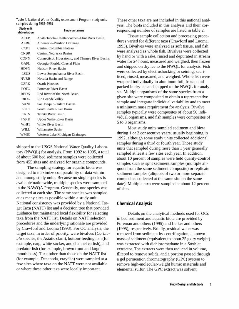
1. National Water-Quality Assessment Program study units sampled during 1992–1995 ........................................ 52. Taxonomic species sampled by the National Water-Quality Assessment Program during 1992–1995 ................ 6

Contents VII
3. Target analytes measured in bed sediment or aquatic biota by the National Water-Quality AssessmentProgram during 1992–1995 ................................................................................................................................... 7
4. Statistical summary of organochlorine concentrations in sediment, 1992–1995 ................................................... 12 5. Statistical summary of organochlorine concentrations in fish, 1992–1995 ............................................................ 136. Statistical summary of organochlorine concentrations in bivalves, 1992–1995..................................................... 14 7. Mean percent composition of selected chlordane constituents and metabolites in technical chlordane and in
sediment and aquatic biota from the National Water-Quality Assessment Program, 1992–1995 ......................... 238. Mean percent composition of
o
,
p
′
- and
p
,
p
′
-DDT and their primary metabolites in technical DDT and in sediment and aquatic biota from the National Water-Quality Assessment Program, 1992–1995 ...... 31
9. Coefficients of determination for linear regressions between concentrations in paired sediment–fish samples ........................................................................................................................................... 36
10. Detection frequencies in sediment, 1992–1995, at censoring levels from 1 to 5
µ
g/kg dry weight....................... 4011. Detection frequencies in sediment, 1992–1995, at censoring levels from 1 to 200
µ
g/kg dry weight................... 4112. Detection frequencies in whole fish, 1992–1995, at censoring levels from 5 to 200
µ
g/kg wet weight ................ 4213. ANOVA of concentration distribution ranks of dieldrin, total chlordane, total DDT, and
total PCBs among land-use classifications for sediment, fish, and bivalves, including Kruskal–Wallis mean scores and Tukey–Kramer multiple comparison tests ......................................................... 44
14. ANOVA of concentration distribution ranks of dieldrin, total chlordane, total DDT, and total PCBs among land-use/basin-size classifications for sediment, fish, and bivalves, including Kruskal–Wallis mean scores and Tukey–Kramer multiple comparison tests ......................................................... 59
15. Sediment-quality guidelines for organochlorine compounds in sediment.............................................................. 7016. Comparison of organochlorine concentrations in sediment with sediment-quality guidelines .............................. 7317. Potential adverse effects on aquatic life at National Water-Quality Assessment Program
sediment sites compared with sites in EPA National Sediment Inventory ............................................................. 7418. Comparison of organochlorine concentrations in whole fish with guidelines for protection of
fish-eating wildlife .................................................................................................................................................. 7519. Comparison of organochlorine concentrations in whole fish with edible-fish guidelines for
protection of human health ..................................................................................................................................... 78
CONVERSION FACTORS and ABBREVIATIONS and ACRONYMS
Conversion Factors
Temperature is given in degrees Celsius (
°
C), which can be converted to degreesFahrenheit (
°
F) by the following equation:
°
F=1.8(
°
C)+32.
Multiply
By To obtain
inch (in.) 2.54 centimeter
foot (ft) 0.3048 meter
mile (mi) 1.609 kilometer
square mile (mi
2
) 2.590 square kilometer

VIII Contents
Abbreviations and Acronyms
(Additional information noted in parentheses)
µ
g/g, microgram per gram
µ
g/kg, microgram per kilogramcm, centimeterg/d, gram per daykg, kilogramkg/d, kilogram per day
km
2
, square kilometermm, millimeter
AET-H, apparent effects threshold–highAET-L, apparent effects threshold–lowANOVA, analysis of varianceEPA, (U.S.) Environmental Protection AgencyER-L, effects range–lowER-M, effects range–medianFDA, (U.S.) Food and Drug AdministrationFWS, (U.S.) Fish and Wildlife ServiceGC, gas chromatographyGC/ECD, gas chromatography with electron capture detectionGIRAS, Geographic Information Retrieval and Analysis SystemGPC, gas permeation chromatographyHCB, hexachlorobenzeneHOC, hydrophobic organic compoundsISQG, (Canadian) interim sediment-quality guidelineMCT, multiple comparison testNAS/NAE, National Academy of Sciences and National Academy of EngineeringNATT, National Target and TaxaNAWQA, National Water-Quality Assessment (Program)NCBP, National Contaminant Biomonitoring ProgramNOAA, National Oceanic and Atmospheric AdministrationNSCRF, National Study of Chemical Residues in FishNS&T, National Status and Trends (Program)NWQL, National Water Quality LaboratoryNYSDEC, New York State Department of Environmental ConservationOC, organochlorine compoundPCA, pentachloranisolePCB, polychlorinated biphenylPEL, probable effect levelPMN, Pesticide Monitoring NetworkSQC, sediment quality criterionSQAL, sediment quality advisory levelTEL, threshold effect levelTEQ, dioxin toxic equivalentUSGS, U.S. Geological Survey

Introduction 1
Organochlorine Pesticides and PCBs in Stream Sediment and Aquatic Biota—Initial Results from the National Water-Quality Assessment Program, 1992–1995
Charles S. Wong, Paul D. Capel, and Lisa H. Nowell
ABSTRACT
One of the goals of the National Water-Quality Assessment (NAWQA) Program of the U.S. Geological Survey is to assess the status and trends in the nation's water quality and to understand the natural and anthropogenic factors that affect water-quality conditions. This report summarizes the occurrence and distribution of 33 organochlorine compounds in fluvial bed sediment and aquatic biota (whole freshwater fish and fresh-water bivalves) sampled by NAWQA investiga-tions between 1991 and 1994. These include historically used insecticides (DDT and metabo-lites, chlordane and its various components, and dieldrin), some currently used pesticides (per-methrin and dacthal) and some industrial chemi-cals and byproducts (PCBs and hexacloro- benzene). Samples were collected at approxi-mately 500 sites in 19 large hydrologic basins throughout the United States. Contaminant levels in bed sediment and aquatic biota are summarized, first on a national basis, and then by land-use clas-sification (for example, urban, cropland, pasture and rangeland, and forest). Nationally, detection frequencies are highest in sediment and biota for the more persistent organochlorine compounds: total DDT, total chlordane, dieldrin, and total PCBs. Organochlorine compounds were detected more frequently in whole fish than in bivalves or bed sediment. Organochlorine pesticide concen-trations were relatively high in agricultural regions with histories of high use. The highest organochlo-rine compound concentrations in both sediment and biota generally were associated with urban
areas. Some organochlorine concentrations in sed-iment exceeded guidelines for the protection of aquatic organisms. A screening-level comparison of measured organochlorine concentrations in whole fish was made with human health guidelines that are applicable to edible fish. This comparison indicates stream sites at which additional sampling of game fish fillets may be warranted, depending on local patterns of fish consumption. A compari-son of current national contaminant levels with previous studies of this scope suggests a gradual decrease in organochlorine contaminant levels, at least in fish.
INTRODUCTION
Hydrophobic organic compounds (HOC) of anthropogenic origin have been produced and used in great quantities over many years. They have been introduced into the hydrologic system via direct dis-charge, atmospheric deposition, and runoff from ter-restrial sources. Because of their hydrophobicity, HOCs sorb readily to particles, which can settle out of the water column to bed sediment, where they can remain for long periods of time. Many HOCs also bio-accumulate within the tissues of aquatic biota. Their persistence in the environment and propensity to accu-mulate in living tissue, coupled with the toxic effects of many HOCs, make them a source of continuing concern to the health of humans and aquatic organ-isms.
This report is a summary of the occurrence and distribution of organochlorine compounds (OC), one class of HOCs, in bed sediment and biota from the first round of intensive sampling by the U.S. Geological

2 OCs and PCBs in Stream Sediment and Aquatic Biota—Initial Results, NAWQA, 1992–1995
Survey’s (USGS) National Water-Quality Assessment (NAWQA) Program. The NAWQA Program is designed to describe the status and trends in the nation’s water quality and to link status and trends with natural and anthropogenic factors that affect them. The study design balances an understanding of the unique nature of each hydrologic system in the program with a nationally consistent design structure. The building blocks of the program are investigations in 55 to 59 major hydrologic basins (study units) in the United States. These study units are divided into three groups, which are intensively studied on a rotational schedule over successive 3-year intervals to provide long-term trends in water quality. Maps of the 59 NAWQA study units are shown in Gilliom and others (1995) and U.S. Geological Survey (1999).
The objectives of the study reported here were (1) to assess the national distribution of OCs in bed sediment and aquatic biota on the basis of results from the first 20 NAWQA study units (1992–1995); (2) to assess differences in OC distributions among the vari-ous media (bed sediment, whole fish, and bivalves) and as a function of land use; (3) to assess trends in OC concentrations by comparing the NAWQA data with results from prior national-scale studies; and (4) to evaluate, to the extent possible, the potential for effects of OC residues on human and ecosystem health.
STUDY DESIGN AND METHODS
Site Selection
There are two general types of NAWQA sites: integrator and indicator sites (Gilliom and others, 1995). Integrator sites are stream sampling sites that are typically located at or near the outlet of large com-plex drainage basins. These sites are chosen to repre-sent stream and river conditions in large heterogeneous basins that are often affected by a com-bination of land-use settings, point sources, and natu-ral influences. Most integrator sites are on major streams and include a large part of the study unit's drainage area, generally from 10 to 100 percent.
Indicator sites are stream sampling sites located at outlets of drainage basins with relatively homoge-neous land-use and physiographic features. In general, the drainage area of an indicator site has more than
half of its drainage area included in the targeted land-use setting. These basins are chosen to be as large as possible while still representing a single setting, and are generally between 50 and 500 km
2
. Samples taken at indicator sites are considered representative of the targeted setting.
Integrator and indicator sites are grouped sepa-rately in the discussion of land-use relations because indicator sites represent drainage basins that are fairly homogeneous with respect to land use, and integrator sites are affected by multiple land uses. Within an indi-vidual study unit, the sites where bed sediment and aquatic biota were sampled typically include the fol-lowing: (1) integrator sites representing the large streams in the study unit, including major nodes in the drainage system; (2) indicator sites representing the principal environmental settings (land areas character-ized by a unique combination of natural and anthropo-genic-related factors, such as row crop cultivation on glacial-till soils); and (3) additional indicator sites with known contamination. One or two reference indi-cator sites were also selected to represent the back-ground conditions where minimal occurrence of OCs was expected. Figures 1 and 2 show the NAWQA study units and the sites for which sediment and biota data were analyzed in this report.
Sample Collection Methods
Samples of sediment and biota were collected from the first 20 study units (table 1) at the same time each year to minimize seasonal variability, generally during summer or autumn low flows. Sediment sample collection and processing methods are described in detail by Shelton and Capel (1994). Briefly, fine-grained surficial bed sediment was collected from sev-eral depositional zones in a stream reach using a hand-held core sampler and then composited into a single sample, resulting in a sample representing the fine-grained surficial sediment in the reach. Ideally, 5 to 10 depositional zones were used, representing left- and right-bank and center-channel depositional zones with different depths of water. A sample from the surficial 2 to 3 cm of sediment in each depositional zone was col-lected in approximate proportion to the size of that depositional zone relative to the other zones repre-sented in the composite. The composite sample was then processed through a 2.0-mm stainless-steel mesh sieve, and one or more aliquots were packed in ice and

Study Design and M
ethods3
0 400 MILES
0 400 KILOMETERS
Bed sediment samping sitesStudy unit
EXPLANATION
Dieldrin concentrationin sediment, microgramsper kilogram dry weight
WILL
CCPT
USNK
NVBR
NVBR
SANJ
TRIN
OZRK
CNBR
SPLT
REDN WMIC
WHIT
ACFB
GAFL
RIOG ALBE
POTO
LSUS
CONN
HDSN
Figure 1.
Map of the first 20 National Water-Quality Assessment Program study units, showing bed sediment sampling sites. Study unit abbreviations are defined in table 1. No data were available for the Potomac River Basin study unit (POTO).

4O
Cs and PCBs in Stream
Sediment and A
quatic Biota—
Initial Results, NA
WQ
A, 1992–1995
WILL
CCPT
USNK
NVBR
NVBR
SANJ
TRIN
OZRK
CNBR
SPLT
REDN WMIC
WHIT
ACFB
GAFL
RIOG ALBE
POTO
LSUS
CONN
HDSN
EXPLANATION
Fish
Bivalves
Study unit
0 400 MILES
0 400 KILOMETERS
Figure 2.
Map of the first 20 National Water-Quality Assessment Program study units, showing sampling sites for fish and bivalves. Study unit abbreviations are defined in table 1. No data were available for the Potomac River Basin study unit (POTO).
Study Design and Methods 5
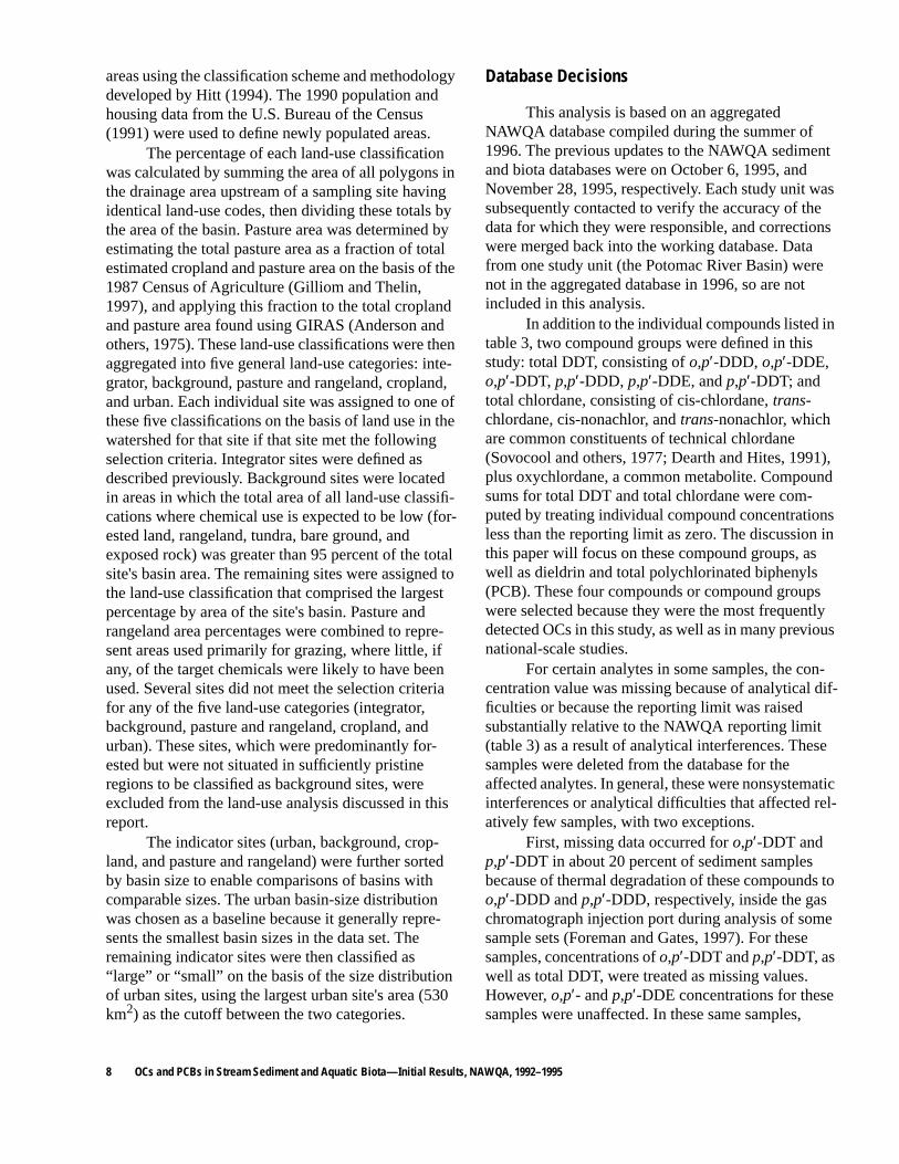
shipped to the USGS National Water Quality Labora-tory (NWQL) for analysis. From 1992 to 1995, a total of about 600 bed sediment samples were collected from 455 sites and analyzed for organic compounds.
The sampling strategy for aquatic biota was designed to maximize comparability of data within and among study units. Because no single species is available nationwide, multiple species were sampled in the NAWQA Program. Generally, one species was collected at each site. The same species was sampled at as many sites as possible within a study unit. National consistency was provided by a National Tar-get Taxa (NATT) list and a decision tree that provided guidance but maintained local flexibility for selecting taxa from the NATT list. Details on NATT selection procedures and the underlying rationale are provided by Crawford and Luoma (1993). For OC analysis, the target taxa, in order of priority, were bivalves (
Corbic-ula
species, the Asiatic clam), bottom-feeding fish (for example, carp, white sucker, and channel catfish), and predator fish (for example, brown trout and large-mouth bass). Taxa other than those on the NATT list (for example, Decapoda, crayfish) were sampled at a few sites where taxa on the NATT were not available or where these other taxa were locally important.
These other taxa are not included in this national anal-ysis. The biota included in this analysis and their cor-responding number of samples are listed in table 2.
Tissue sample collection and processing proce-dures varied for different taxa (Crawford and Luoma, 1993). Bivalves were analyzed as soft tissue, and fish were analyzed as whole fish. Bivalves were collected by hand or with a rake, rinsed and depurated in stream water for 24 hours, measured and weighed, then frozen and shipped on dry ice to the NWQL for analysis. Fish were collected by electroshocking or seining, sacri-ficed, rinsed, measured, and weighed. Whole fish were wrapped individually in aluminum foil, frozen and packed in dry ice and shipped to the NWQL for analy-sis. Multiple organisms of the same species from a given site were composited to obtain a representative sample and integrate individual variability and to meet a minimum mass requirement for analysis. Bivalve samples typically were composites of about 50 indi-vidual organisms, and fish samples were composites of 5 to 8 organisms.
Most study units sampled sediment and biota during 1 or 2 consecutive years, usually beginning in 1992, although some study units collected additional samples during a third or fourth year. Those study units that sampled during more than 1 year generally sampled at least a few sites each year. In addition, about 10 percent of samples were field quality-control samples such as split sediment samples (multiple ali-quots from the same sediment composite) or replicate sediment samples (aliquots of two or more separate composites collected at the same site on the same date). Multiple taxa were sampled at about 12 percent of sites.
Chemical Analysis
Details on the analytical methods used for OCs in bed sediment and aquatic biota are provided by Foreman and others (1995) and Leiker and others (1995), respectively. Briefly, residual water was removed from sediment by centrifugation, a known mass of sediment (equivalent to about 25 g dry weight) was extracted with dichloromethane in a Soxhlet extractor. The extracts were then reduced in volume, filtered to remove solids, and a portion passed through a gel permeation chromatography (GPC) system to remove high-molecular-weight humic materials and elemental sulfur. The GPC extract was solvent
Table 1.
National Water-Quality Assessment Program study units sampled during 1992–1995
Study unit abbreviation
Study unit name
ACFB Apalachicola–Chattahoochee–Flint River Basin
ALBE Albemarle–Pamlico Drainage
CCPT Central Columbia Plateau
CNBR Central Nebraska Basins
CONN Connecticut, Housatonic, and Thames River Basins
GAFL Georgia–Florida Coastal Plain
HDSN Hudson River Basin
LSUS Lower Susquehanna River Basin
NVBR Nevada Basin and Range
OZRK Ozark Plateaus
POTO Potomac River Basin
REDN Red River of the North Basin
RIOG Rio Grande Valley
SANJ San Joaquin–Tulare Basins
SPLT South Platte River Basin
TRIN Trinity River Basin
USNK Upper Snake River Basin
WHIT White River Basin
WILL Willamette Basin
WMIC Western Lake Michigan Drainages

6 OCs and PCBs in Stream Sediment and Aquatic Biota—Initial Results, NAWQA, 1992–1995
exchanged to hexane, cleaned up and fractionated using alumina/silica adsorption chromatography, and analyzed using gas chromatography with electron cap-ture detection (GC/ECD). Target analytes and their reporting limits are listed in table 3. Organic and inor-ganic carbon in sediment was determined by induction furnace oxidation and subsequent thermal conductivity measurement of evolved carbon dioxide (Wershaw and others, 1987).
Frozen composite whole-body tissue samples were homogenized (Leiker and others, 1995). A sam-ple of the tissue composite was dried by mixing with anhydrous sodium sulfate and extracted with dichlo-
romethane in a Soxhlet apparatus. An aliquot was then removed for percent lipid determination. A portion of the extract was passed through a GPC system to remove lipids and other interferences. This extract was then solvent-exchanged into hexane, fractionated by alumina/silica adsorption chromatography, and ana-lyzed by GC/ECD. Target analytes and their reporting limits are listed in table 3. Lipid content in tissue sam-ples was determined gravimetrically.
Approximately 10 to 20 percent of samples run were laboratory quality assurance samples (spiked samples, standard reference material samples, various blanks, and other standard solutions). Analytical
Table 2.
Taxonomic species sampled by the National Water-Quality Assessment Program during 1992–1995
[Taxon level: F, family; G, genus; S, species. Biota type: F, fish; B, bivalve]
Common name Scientific nameTaxonlevel
Biotatype
Number of samples
Mussels
Unionidae
F B 1
Threeridge
Amblema plicata
S B 1
Asiatic clam
Corbicula
G B 47
Asiatic clam
Corbicula manilensis
S B 71
Cutthroat trout
Oncorhynchus clarki
S F 1
Rainbow trout
Oncorhynchus mykiss
S F 2
Brown trout
Salmo trutta
S F 3
Mountain whitefish
Prosopium williamsoni
S F 1
Common carp
Cyprinus carpio
S F 39
Longnose sucker
Catostomus catostomus
S F 1
White sucker
Catostomus commersoni
S F 101
Largescale sucker
Catostomus macrocheilus
S F 6
Bridgelip sucker
Catostomus columbianus
S F 5
Utah sucker
Catostomus ardens
S F 10
Mountain sucker
Catostomus platyrhynchus
S F 1
River carpsucker
Carpiodes carpio
S F 2
Black redhorse
Moxostoma duquesnei
S F 1
Northern hog sucker
Hypentelium nigricans
S F 3
Blue catfish
Ictalurus furcatus
S F 3
Channel catfish
Ictalurus punctatus
S F 2
Yellow bullhead
Ameiurus natalis
S F 2
Eastern mosquitofish
Gambusia holbrooki
S F 3
Sculpins
Cottus
G F 13
Mottled sculpin
Cottus bairdi
S F 0
Paiute sculpin
Cottus beldingi
S F 3
Wood River sculpin
Cottus leiopomus
S F 1
Rock bass
Ambloplites rupestris
S F 5
Redbreast sunfish
Lepomis auritus
S F 8
Bluegill
Lepomis macrochirus
S F 2
Longear sunfish
Lepomis megalotis
S F 11
Smallmouth bass
Micropterus dolomieu
S F 3
Largemouth bass
Micropterus salmoides
S F 2

Study Design and Methods 7
method performance and quality assurance/quality control are discussed by Foreman and others (1995) and Leiker and others (1995). Field samples were ana-lyzed in sets of 11 samples, with each set also includ-ing one reagent spike sample to represent optimum method performance for that set, one laboratory blank sample, one laboratory duplicate sample, and one stan-dard reference material. In addition, surrogate com-pounds consisting of OCs not found in environmental samples were added to all field samples and quality assurance samples to monitor methodological errors in individual samples.
Land-Use Classifications
Each watershed, represented by a sampling site, was classified by its general land-use characteristics determined from the Geographic Information Retrieval and Analysis System (GIRAS) land-use/land-cover (1:250,000 scale) maps from the 1970s, using the Level II classification scheme (Anderson and others, 1975). These coverages were generated by superimposing the land-use/land-cover information for the study unit on the basin boundary. Land-use classi-fications were updated for “new residential urban”
Table 3.
Target analytes measured in bed sediment or aquatic biota by the National Water-Quality Assessment Program during 1992–1995
[Compound group: The compound group name is listed for each analyte included in the four most commonly detected compounds or com-pound groups: CHL, total chlordane; DDT, total DDT; DIEL, dieldrin; PCB, total polychlorinated biphenyls; blank cell indicates this ana-lyte is not among the most commonly detected compounds or compound groups. CAS, Chemical Abstracts Service;
µ
g/kg, microgram per kilogram; mg/L, milligram per liter; K
ow
,
n
-octanol-water partition coefficient; na, not analyzed; —, not available]
1
From Nowell and others, 1999.
Chemical nameCAS registry
number
Reporting limitWater
solubility
1
(mg/L)
Log
K
ow1
Estimated soil
half-life
1
(days)
Compound
groupBiota
(
µ
g/kg
[wet])
Sediment
(
µ
g/kg
[dry])
Aldrin 309-00-2 5 1 0.027 — 365Chloroneb 2675-77-6 na 5 8 — 130
cis
-Chlordane 5103-71-9 5 1 0.06 6 365 CHL
trans
-Chlordane 5103-74-2 5 1 0.06 6 365 CHLDacthal 1861-32-1 5 5 0.5 4-5 50
o
,
p
′
-DDD 53-19-0 5 1 0.1 5.1–6.2 730–5,700 DDT
p
,
p
′
-DDD 72-54-8 5 1 0.05 5.1–6.2 730–5,700 DDT
o
,
p
′
-DDE 3424-82-6 5 1 0.065 5.7–7.0 730–5,700 DDT
p
,
p
′
-DDE 72-55-9 5 1 0.065 5.7–7.0 730–5,700 DDT
o
,
p
′
-DDT 789-02-6 5 2 — 6 2,400 DDT
p
,
p
′
-DDT 50-29-3 5 2 0.0077 6 110–5,500 DDTDieldrin 60-57-1 5 1 0.14 3.7–6.2 1,000 DIELEndosulfan I 959-98-8 na 1 0.32 3.1 4–200Endrin 72-20-8 5 2 0.24 3.2–5.3 4,300
α
-HCH 319-84-6 5 1 1.63 3.8 2–19
β
-HCH 319-85-7 5 1 — — —
γ
-HCH (Lindane) 58-89-9 5 1 7 3.4 100–1,400
δ
-HCH 319-86-8 5 na — — —Heptachlor 76-44-8 5 1 0.056 4.4–5.5 250Heptachlor epoxide 1024-57-3 5 1 0.3 3.6 5–79 CHLHexachlorobenzene 118-74-1 5 50 0.04 3.9–6.4 1,000Isodrin 465-73-6 na 1 — — —
o
,
p
′
-Methoxychlor 30667-99-3 5 5 — — —
p
,
p
′
-Methoxychlor 72-43-5 5 5 0.1 4.7 7–210Mirex 2385-85-5 5 1 0.00007 6.9 3,000
cis
-Nonachlor 5103-73-1 5 1 0.06 5.7 — CHL
trans
-Nonachlor 39765-80-5 5 1 0.06 5.7 — CHLOxychlordane 27304-13-8 5 1 200 2.6 — CHLTotal PCBs — 50 100 — — — PCBPentachloroanisole 1825-21-4 5 50 0.2 5.7 —
cis
-Permethrin 61949-76-6 na 5 0.006 6.1 42
trans
-Permethrin 61949-77-7 na 5 0.006 6.1 42Toxaphene 8001-35-2 200 200 3 3.3 9
8 OCs and PCBs in Stream Sediment and Aquatic Biota—Initial Results, NAWQA, 1992–1995
areas using the classification scheme and methodology developed by Hitt (1994). The 1990 population and housing data from the U.S. Bureau of the Census (1991) were used to define newly populated areas.
The percentage of each land-use classification was calculated by summing the area of all polygons in the drainage area upstream of a sampling site having identical land-use codes, then dividing these totals by the area of the basin. Pasture area was determined by estimating the total pasture area as a fraction of total estimated cropland and pasture area on the basis of the 1987 Census of Agriculture (Gilliom and Thelin, 1997), and applying this fraction to the total cropland and pasture area found using GIRAS (Anderson and others, 1975). These land-use classifications were then aggregated into five general land-use categories: inte-grator, background, pasture and rangeland, cropland, and urban. Each individual site was assigned to one of these five classifications on the basis of land use in the watershed for that site if that site met the following selection criteria. Integrator sites were defined as described previously. Background sites were located in areas in which the total area of all land-use classifi-cations where chemical use is expected to be low (for-ested land, rangeland, tundra, bare ground, and exposed rock) was greater than 95 percent of the total site's basin area. The remaining sites were assigned to the land-use classification that comprised the largest percentage by area of the site's basin. Pasture and rangeland area percentages were combined to repre-sent areas used primarily for grazing, where little, if any, of the target chemicals were likely to have been used. Several sites did not meet the selection criteria for any of the five land-use categories (integrator, background, pasture and rangeland, cropland, and urban). These sites, which were predominantly for-ested but were not situated in sufficiently pristine regions to be classified as background sites, were excluded from the land-use analysis discussed in this report.
The indicator sites (urban, background, crop-land, and pasture and rangeland) were further sorted by basin size to enable comparisons of basins with comparable sizes. The urban basin-size distribution was chosen as a baseline because it generally repre-sents the smallest basin sizes in the data set. The remaining indicator sites were then classified as “large” or “small” on the basis of the size distribution of urban sites, using the largest urban site's area (530 km
2
) as the cutoff between the two categories.
Database Decisions
This analysis is based on an aggregated NAWQA database compiled during the summer of 1996. The previous updates to the NAWQA sediment and biota databases were on October 6, 1995, and November 28, 1995, respectively. Each study unit was subsequently contacted to verify the accuracy of the data for which they were responsible, and corrections were merged back into the working database. Data from one study unit (the Potomac River Basin) were not in the aggregated database in 1996, so are not included in this analysis.
In addition to the individual compounds listed in table 3, two compound groups were defined in this study: total DDT, consisting of
o
,
p
′
-DDD,
o
,
p
′
-DDE,
o
,
p
′
-DDT,
p
,
p
′
-DDD,
p
,
p
′
-DDE, and
p
,
p
′
-DDT; and total chlordane, consisting of cis-chlordane,
trans
-chlordane, cis-nonachlor, and
trans
-nonachlor, which are common constituents of technical chlordane (Sovocool and others, 1977; Dearth and Hites, 1991), plus oxychlordane, a common metabolite. Compound sums for total DDT and total chlordane were com-puted by treating individual compound concentrations less than the reporting limit as zero. The discussion in this paper will focus on these compound groups, as well as dieldrin and total polychlorinated biphenyls (PCB). These four compounds or compound groups were selected because they were the most frequently detected OCs in this study, as well as in many previous national-scale studies.
For certain analytes in some samples, the con-centration value was missing because of analytical dif-ficulties or because the reporting limit was raised substantially relative to the NAWQA reporting limit (table 3) as a result of analytical interferences. These samples were deleted from the database for the affected analytes. In general, these were nonsystematic interferences or analytical difficulties that affected rel-atively few samples, with two exceptions.
First, missing data occurred for
o
,p′-DDT and p,p′-DDT in about 20 percent of sediment samples because of thermal degradation of these compounds to o,p′-DDD and p,p′-DDD, respectively, inside the gas chromatograph injection port during analysis of some sample sets (Foreman and Gates, 1997). For these samples, concentrations of o,p′-DDT and p,p′-DDT, as well as total DDT, were treated as missing values. However, o,p′- and p,p′-DDE concentrations for these samples were unaffected. In these same samples,

Study Design and Methods 9
thermal degradation of some less commonly detected analytes (for example, o,p′ and p,p′-methoxychlor) also occurred.
The second exception involved total PCBs in sediment, which were analyzed at a reporting limit of 100 µg/kg dry weight in some samples and at 50 µg/kg dry weight in other samples (table 3). The higher reporting limit was generally used for samples col-lected early in the study. For consistency, the higher limit was used in data analysis for all PCB measure-ments in this report. Therefore, samples that were ana-lyzed at a 50 µg/kg reporting limit and had concentrations between 50 and 100 µg/kg (dry weight) were considered to be nondetections (less than the 100 µg/kg reporting limit) in this analysis.
In computing total DDT, the concentrations of all constituents for which data were available (all non-missing values) were summed unless one or more of the p,p′ isomers, which are the major components of total DDT, were reported as missing, in which case the total DDT value for that site also was regarded as missing. Total chlordane was computed in a similar manner, in that the total chlordane value was regarded as missing if one or more of the major components (cis- and trans-chlordane, cis- and trans-nonachlor) were missing. If oxychlordane was the only compo-nent of total chlordane missing, then total chlordane was computed as the sum of the four major compo-nents.
The database originally included many sites at which multiple samples were collected in different years, as well as field replicate samples collected for quality control purposes. Many of the statistics pre-sented in this study apply to groupings of sites, either nationally (that is, the entire data set), or on the basis of a specific characteristic, such as land use (for exam-ple, urban sites or agricultural sites). For this analysis, to prevent multiple-year or replicate samples from unduly weighting statistics towards certain sites, one sample was selected to represent each site at which multiple samples were collected. These representative samples were selected using specific criteria.
The selection criteria for sediment were as fol-lows:
• If one or more samples at a given site had miss-ing data for the DDT compounds, chlordane compounds, dieldrin, or PCBs (table 3), then
the choice was made from among the other samples.
• If one sample had no sediment organic carbon data associated with it, then the choice was made from among the other samples.
• Samples that had sediment organic carbon val-ues associated with them were selected over those that had an organic carbon value mea-sured at the same site but on another date.
• If the samples of a site were equivalent in com-pleteness of data for the four compound groups listed above and in quality of sedi-ment organic carbon data, then the sample with the earliest sampling date or time was selected.
In the final database analyzed in this study, 56 percent of sediment samples from the entire data set are from 1992, 28 percent are from 1993, 14 percent are from 1994, and 2 percent are from 1995.
For biota, the data for fish samples were ana-lyzed separately from the data for bivalves. The selec-tion criteria for choosing biota were as follows:
• If a site had both fish and bivalve samples, then one sample of each type was retained for analysis.
• If one or more samples at a given site had miss-ing data for the DDT compounds, chlordane compounds, dieldrin, or PCBs (table 3), then the choice was made from among the other samples.
• For sites with multiple bivalve samples, the sample from the earliest date or time of sam-pling was selected.
• For sites with multiple fish samples, the sample from the earliest date or time of sampling was selected if all samples were from the same taxon.
• If more than one fish taxon was sampled at that site, the samples from the earliest year of sampling were selected. Among these sam-ples, the taxon most commonly sampled in the study unit (usually the most common spe-cies nationally, table 2) was selected. If more than one sample of this taxon was sampled during the earliest sampling year, then the sample from the earliest date or time of sam-pling was selected.
In the final database analyzed in this study, 79 percent of bivalve samples were from 1992, 18 percent were from 1993, and 3 percent were from 1994. Of fish

10 OCs and PCBs in Stream Sediment and Aquatic Biota—Initial Results, NAWQA, 1992–1995
samples, 62 percent of samples were from 1992, 23 percent were from 1993, and 15 percent were from 1994.
NATIONAL OVERVIEW
Statistical Summary
Summary statistics were compiled on the 485 total sites in the national data set, of which 455 sites had bed sediment data, 234 sites had fish data, and 120 sites had bivalve data. The detection frequency of a given compound is defined as the total number of sam-ples with detectable residues of that compound divided by the total number of samples analyzed for that compound. Detection frequencies for individual target analytes are summarized in figure 3, and con-centration percentiles summarizing the distributions of contaminant concentrations are summarized for sedi-ment, fish, and bivalves in tables 4, 5, and 6, respec-tively. As will be discussed below, the data shown in figure 3 have not been censored to a common reporting limit among the target analytes. Therefore, detection frequencies will reflect differences in individual reporting limits, as well as environmental occurrence. Certain analytes have much higher reporting limits, so their detection frequencies are not directly comparable to other analytes that have lower reporting limits. In sediment, most analytes have reporting limits of 1 to 5 µg/kg dry weight (table 3); the exceptions are hexachlorobenzene (HCB), pentachloroanisole (PCA), total PCBs, and toxaphene, which have reporting lim-its of 50, 50, 100, and 200 µg/kg dry weight, respec-tively. In fish, most analytes have reporting limits of 5 µg/kg wet weight, except for total PCBs and tox-aphene, which have reporting limits of 50 and 200 µg/kg wet weight, respectively (table 3).
Detection frequencies among media generally were highest in fish (table 5 and fig. 3), lower in sedi-ment (table 4 and fig. 3), and much lower in bivalves (table 6 and fig. 3). The most commonly detected com-pounds were DDT isomers and their DDD and DDE analogues, total PCBs, dieldrin, and compounds in the chlordane group (cis- and trans-chlordane, and cis- and trans-nonachlor). The compound with the highest detection frequencies in all three types of sam-pling media was p,p′-DDE, which was detected in fish at 80 percent (table 5), in sediment at 39 percent (table
4), and in bivalves at 29 percent (table 6) of sites. All of the p,p′ isomers of DDT and its metabolites were detected more frequently than the o,p′ isomers, which is reflective of the higher ratio of p,p′-DDT to o,p′-DDT in technical grade DDT (World Health Organization, 1989).
The detection frequency for total PCBs in sedi-ment (5.8 percent of sites [table 4]) is rather low. This seems to contradict previous studies that have found PCBs ubiquitously in the environment (Erickson, 1997). The low detection frequency for PCBs in sedi-ment in this study is due to the relatively high report-ing limit (100 µg/kg dry weight), which is higher than the PCB levels found in sediment from remote regions away from known point sources (Jeremiason and oth-ers, 1994).
Concentration distributions of the four most commonly detected compounds or compound groups are shown in cumulative frequency diagrams (fig. 4). In general, concentrations and detection frequencies (the percentage of samples above any given concentra-tion) of total DDT and total PCBs tend to be higher than those of dieldrin and total chlordane (fig. 4). Con-centrations and detection frequencies in fish also tend to be higher than concentrations in sediment or bivalves. Figures 5 and 6 show concentration distribu-tions for the principal components of total DDT and the components of total chlordane, respectively. Con-centrations and detection frequencies of these individ-ual analytes are generally higher in fish than in sediment or bivalves, except that the maximum con-centrations of p,p′-DDE and p,p′-DDT in bivalves (1,600 and 580 µg/kg wet weights, respectively) are fairly comparable to those in fish (2,400 and 430 µg/kg wet weight, respectively).
Direct comparison of detection frequencies observed by different studies is problematic because of differences between studies in analytical methods and reporting limits. In addition, measured concentrations and detection frequencies are affected by study design features such as sampling protocols, site selection strategy, and the period (month and year) of sampling. Nonetheless, the relatively high frequencies of detec-tion for DDT and metabolites, chlordane components, dieldrin, and PCBs in the present study agree with the detection history of these compounds in prior studies undertaken during the last 30 years.
The first national effort to monitor pesticides in bed sediment was the Pesticide Monitoring Network

National O
verview11
Per
cent
of s
ites
with
det
ecta
ble
resi
dues
100
90
80
70
60
50
40
30
20
10
0
fish
bivalves
sediment
p,p�
-DD
E
p,p�
-DD
D
p,p�
-DD
T
p,p�
-met
hoxy
chlo
r
o,p�
-met
hoxy
chlo
r
hept
achl
or
endo
sulta
n
o,p�
-DD
D
o,p�
-DD
T
o,p�
-DD
E
tota
l PC
Bs
tran
s-no
nach
lor
cis-
chlo
rdan
e
tran
s-ch
lord
ane
cis-
nona
chlo
r
cis-
perm
ethr
in
tran
s-pe
rmet
hrin
diel
drin
oxyc
hlor
dane
hexa
chlo
robe
nzen
e
�-H
CH
�-H
CH
�-H
CH
hept
achl
or e
poxi
de
dact
hal
aldr
in
�-H
CH
endr
in
chlo
rone
b
mire
x
isod
rin
toxa
phen
e
pent
achl
oran
isol
e
Figure 3. Detection frequencies (percentage of sites with detectable residues) of target analytes in sediment, fish, and bivalves. The data shown have not been censored to a common reporting limit. Reporting limits for individual analytes are given in table 2.

12 OCs and PCBs in Stream Sediment and Aquatic Biota—Initial Results, NAWQA, 1992–1995
(PMN), operated by the USGS and U.S. Environmen-tal Protection Agency (EPA) as part of the interagency National Pesticide Monitoring Program (Gilliom and others, 1985). The USGS collected whole water and bed sediment samples at 160–180 sites on major rivers throughout the United States, and the EPA analyzed them for pesticides. Bed sediment data for 1975 to
1980 were analyzed by Gilliom and others (1985). Surficial bed sediment samples were collected along a cross-section of a river and composited, then analyzed unsieved. Target analytes in bed sediment included organochlorine and organophosphate insecticides, and a few herbicides. The most commonly detected pesti-cides in the PMN were DDT and metabolites (detected
Table 4. Statistical summary of organochlorine concentrations in sediment, 1992–1995
[All statistics apply to samples in the national data set. Compounds are listed in order of detection frequency in fish shown in table 5. Frequency of detection: percentage of samples with concentrations at or above the reporting limit. PCB, polychlori-nated biphenyl; RL, reporting limit in microgram per kilogram dry weight; µg/kg, microgram per kilogram; <, less than]
1Total PCBs censored at a reporting limit of 100 µg/kg dry weight. 2Total PCBs censored at a reporting limit of 50 µg/kg dry weight.
Target
analyte
Number
of
samples
Concentration (µg/kg dry weight) at given percentile Frequency
of detection
(percent)RL 5 10 25 50 75 90 95 100
p,p′-DDE 421 1 <1 <1 <1 <1 2.2 7.28 12.9 220 39.4
Total PCBs1 428 100 <100 <100 <100 <100 <100 <100 145.5 13,000 5.8
Total PCBs2 207 50 <50 <50 <50 <50 <50 150 336 13,000 18.8
p,p′-DDD 350 1 <1 <1 <1 <1 <1 4.19 9.24 130 24.9
trans-Nonachlor 411 1 <1 <1 <1 <1 <1 2.08 3 18 15.8
p,p′-DDT 358 2 <2 <2 <2 <2 <2 4.03 12.05 180 18.7
Dieldrin 413 1 <1 <1 <1 <1 <1 1.5 3.23 18 14.3
cis-Chlordane 411 1 <1 <1 <1 <1 <1 1.8 3.3 17 15.8
cis-Nonachlor 412 1 <1 <1 <1 <1 <1 <1 1.6 10 9.2
trans-Chlordane 416 1 <1 <1 <1 <1 <1 2.2 3.775 20 17.1
Oxychlordane 405 1 <1 <1 <1 <1 <1 <1 <1 1.3 0.3
o,p′-DDD 350 1 <1 <1 <1 <1 <1 <1 2.09 150 10.9
Pentachloroanisole 430 50 <50 <50 <50 <50 <50 <50 <50 <50 0
Hexachlorobenzene 442 50 <50 <50 <50 <50 <50 <50 <50 <50 0
o,p′-DDT 354 2 <2 <2 <2 <2 <2 <2 <2 30 3.1
Heptachlor epoxide 412 1 <1 <1 <1 <1 <1 <1 <1 4.6 1.2
o,p′-DDE 405 1 <1 <1 <1 <1 <1 <1 <1 22 2
γ-HCH 413 1 <1 <1 <1 <1 <1 <1 <1 5.2 1
Dacthal 414 5 <5 <5 <5 <5 <5 <5 <5 25 1.5
Endrin 412 2 <2 <2 <2 <2 <2 <2 <2 <2 0
α-HCH 415 1 <1 <1 <1 <1 <1 <1 <1 <1 0
Toxaphene 419 200 <200 <200 <200 <200 <200 <200 <200 240 0.2
Aldrin 418 1 <1 <1 <1 <1 <1 <1 <1 3 0.5
Mirex 418 1 <1 <1 <1 <1 <1 <1 <1 4.4 1.9
p,p′-Methoxychlor 378 5 <5 <5 <5 <5 <5 <5 <5 71 0.8
o,p′-Methoxychlor 382 5 <5 <5 <5 <5 <5 <5 <5 <5 0
β-HCH 411 1 <1 <1 <1 <1 <1 <1 <1 1.2 0.5
Heptachlor 419 1 <1 <1 <1 <1 <1 <1 <1 <1 0.2
Endosulfan 409 1 <1 <1 <1 <1 <1 <1 <1 8.8 2.7
cis-Permethrin 344 5 <5 <5 <5 <5 <5 <5 <5 26 1.2
trans-Permethrin 340 5 <5 <5 <5 <5 <5 <5 <5 15 0.9
Chloroneb 396 5 <5 <5 <5 <5 <5 <5 <5 <5 0
Isodrin 409 1 <1 <1 <1 <1 <1 <1 <1 <1 0

National Overview 13
in 9–17 percent of samples), chlordane (10 percent), and dieldrin (12 percent). In coastal and estuarine areas, surficial sediment was sampled by the National Oceanic and Atmospheric Administration’s (NOAA) National Status and Trends (NS&T) Program for Marine Environmental Quality to determine the geo-graphic distribution of OC contaminants (National Oceanic and Atmospheric Administration, 1988, 1989, 1991). This nationwide study found frequent detec-tions of total DDT (detected in 83 percent of samples), as well as total chlordane (61 percent), HCB (50 per-cent), and dieldrin (48 percent) in coastal and marine sediment. The detection frequencies from the NS&T
program are somewhat higher than in the present study. HCB was not detected in sediment in the present study because of its high analytical reporting limit (50 µg/kg dry weight).
For biota, the U.S. Fish and Wildlife Service (FWS) analyzed organochlorine compounds in whole freshwater fish nationwide from 1967 to 1986, as part of the National Contaminant Biomonitoring Program (NCBP), to focus on potential threats to fish and wild-life resources (Henderson and others, 1969, 1971; Schmitt and others, 1981, 1983, 1985, 1990). For the years 1976 to 1984, the NCBP detected total DDT in 97–100 percent of samples, total chlordane in 73–87
Table 5. Statistical summary of organochlorine concentrations in fish, 1992–1995
[All statistics apply to samples in the national data set. Compounds are listed in order of detection frequency. Frequency of detection: percentage of samples with concentrations at or above the reporting limit. PCB, polychlorinated biphenyl; RL, reporting limit in microgram per kilogram wet weight; µg/kg, microgram per kilogram; <, less than]
Target
analyte
Number
of
samples
Concentration (µg/kg wet weight) at given percentile Frequency
of
detection
(percent)RL 5 10 25 50 75 90 95 100
p,p′-DDE 233 5 <5 <5 6.9 27 80.5 186 326 2,400 79.8
Total PCBs 233 50 <50 <50 <50 <50 150 646 1,400 72,000 44.6
p,p′-DDD 224 5 <5 <5 <5 <5 14 33.5 46 1,200 42.4
trans-Nonachlor 231 5 <5 <5 <5 <5 9.2 21.8 29.4 120 33.8
p,p′-DDT 232 5 <5 <5 <5 <5 7.08 21.7 30.35 430 32.3
Dieldrin 232 5 <5 <5 <5 <5 6.15 21 36.05 260 28.9
cis-Chlordane 231 5 <5 <5 <5 <5 <5 15.8 28.8 150 24.2
cis-Nonachlor 230 5 <5 <5 <5 <5 <5 8.59 11.45 53 18.7
trans-Chlordane 232 5 <5 <5 <5 <5 <5 8.61 15.35 56 16.8
Oxychlordane 232 5 <5 <5 <5 <5 <5 5.77 11.35 30 12.1
o,p′-DDD 231 5 <5 <5 <5 <5 <5 <5 8.82 360 9.5
Pentachloroanisole 232 5 <5 <5 <5 <5 <5 <5 7.56 87 8.2
Hexachlorobenzene 234 5 <5 <5 <5 <5 <5 <5 8.875 33 7.3
o,p′-DDT 228 5 <5 <5 <5 <5 <5 <5 5.2 140 5.7
Heptachlor epoxide 232 5 <5 <5 <5 <5 <5 <5 7.335 24 5.6
o,p′-DDE 227 5 <5 <5 <5 <5 <5 <5 5.06 130 4.9
γ-HCH 231 5 <5 <5 <5 <5 <5 <5 <5 30 4.3
Dacthal 231 5 <5 <5 <5 <5 <5 <5 <5 67 3
Endrin 232 5 <5 <5 <5 <5 <5 <5 <5 16 1.7
δ-HCH 230 5 <5 <5 <5 <5 <5 <5 <5 5.5 0.4
α-HCH 232 5 <5 <5 <5 <5 <5 <5 <5 5.4 0.4
Toxaphene 233 200 <200 <200 <200 <200 <200 <200 <200 210 0.4
Aldrin 233 5 <5 <5 <5 <5 <5 <5 <5 <5 0
Mirex 233 5 <5 <5 <5 <5 <5 <5 <5 <5 0
p,p′-Methoxychlor 233 5 <5 <5 <5 <5 <5 <5 <5 <5 0
o,p′-Methoxychlor 231 5 <5 <5 <5 <5 <5 <5 <5 <5 0
β-HCH 232 5 <5 <5 <5 <5 <5 <5 <5 <5 0
Heptachlor 233 5 <5 <5 <5 <5 <5 <5 <5 <5 0

14 OCs and PCBs in Stream Sediment and Aquatic Biota—Initial Results, NAWQA, 1992–1995
percent of samples, dieldrin in 61–75 percent of sam-ples, and toxaphene in 46–73 percent of samples each year. Less frequently detected compounds in the NCBP include total heptachlor (27–38 percent of sam-ples each year), endrin (16–26 percent of samples), HCB (13–21 percent of samples), lindane (6–29 per-cent of samples), and mirex (7–10 percent of samples). Another study, the EPA’s National Study of Chemical Residues in Fish (NSCRF), measured contaminants in whole fish and fish fillets (mostly freshwater) nation-wide during 1986–1987 (U.S. Environmental Protec-tion Agency, 1992a,b). The most commonly detected pesticides (or pesticide metabolites) in the NSCRF
were DDE (detected in 98 percent of samples), trans-nonachlor (72 percent of samples), cis- and trans-chlo-rdane (59 and 54 percent of samples, respectively), dieldrin (56 percent of samples), and pentachloroani-sole (54 percent of samples). The observations from these previous large-scale studies generally agree with the results from the present study, except that detection frequencies from previous studies generally are slightly higher than in the present study for most ana-lytes.
In addition, estuarine fish and bivalves were analyzed for pesticides as part of two large-scale stud-ies of coastal and estuarine areas. First, the Bureau of
Table 6. Statistical summary of organochlorine concentrations in bivalves, 1992–1995
[All statistics apply to samples in the national data set. Compounds are listed in order of detection frequency in fish shown in table 5. Frequency of detection: percentage of samples with concentrations at or above the reporting limit. PCB, polychlori-nated biphenyl; RL, reporting limit in microgram per kilogram dry weight; µg/kg, microgram per kilogram; <, less than]
Target
analyte
Number
of
samples
Concentration (µg/kg wet weight) at given percentile Frequency
of detection
(percent)RL 5 10 25 50 75 90 95 100
p,p′-DDE 120 5 <5 <5 <5 <5 5.3 15.8 32.45 1,600 29.2
Total PCBs 120 50 <50 <50 <50 <50 <50 <50 82.95 6,700 7.5
p,p′-DDD 119 5 <5 <5 <5 <5 <5 <5 <5 100 5
trans-Nonachlor 118 5 <5 <5 <5 <5 <5 <5 9.575 17 9.3
p,p′-DDT 120 5 <5 <5 <5 <5 <5 <5 9.38 580 5.8
Dieldrin 119 5 <5 <5 <5 <5 <5 <5 7.9 20 7.6
cis-Chlordane 119 5 <5 <5 <5 <5 <5 <5 7.1 15 7.6
cis-Nonachlor 120 5 <5 <5 <5 <5 <5 <5 <5 9.9 2.5
trans-Chlordane 120 5 <5 <5 <5 <5 <5 <5 7.99 16 7.5
Oxychlordane 120 5 <5 <5 <5 <5 <5 <5 <5 <5 0
o,p′-DDD 118 5 <5 <5 <5 <5 <5 <5 <5 20 1.7
Pentachloroanisole 120 5 <5 <5 <5 <5 <5 <5 <5 <5 0
Hexachlorobenzene 120 5 <5 <5 <5 <5 <5 <5 <5 <5 0
o,p′-DDT 119 5 <5 <5 <5 <5 <5 <5 <5 36 1.7
Heptachlor epoxide 120 5 <5 <5 <5 <5 <5 <5 <5 <5 0
o,p′-DDE 119 5 <5 <5 <5 <5 <5 <5 <5 22 3.4
γ-HCH 120 5 <5 <5 <5 <5 <5 <5 <5 <5 0
Dacthal 120 5 <5 <5 <5 <5 <5 <5 <5 360 3.3
Endrin 120 5 <5 <5 <5 <5 <5 <5 <5 <5 0
δ-HCH 120 5 <5 <5 <5 <5 <5 <5 <5 <5 0
α-HCH 120 5 <5 <5 <5 <5 <5 <5 <5 <5 0
Toxaphene 120 200 <200 <200 <200 <200 <200 <200 <200 2,000 1.7
Aldrin 120 5 <5 <5 <5 <5 <5 <5 <5 <5 0
Mirex 120 5 <5 <5 <5 <5 <5 <5 <5 <5 0
p,p′-Methoxychlor 120 5 <5 <5 <5 <5 <5 <5 <5 <5 0
β-HCH 120 5 <5 <5 <5 <5 <5 <5 <5 6 1.7
Heptachlor 120 5 <5 <5 <5 <5 <5 <5 <5 <5 0

National Overview 15
10
0
20
30
40
50
60
70
80
90
100
20
30
40
50
60
70
80
90
10
20
30
40
50
1 10 100 1,000 10,000 100,000
Concentration, in micrograms per kilogram, in wet weight
dieldrintotal chlordanetotal DDTtotal PCBs
10
0
100
0
60
70
80
90
100
Per
cent
age
of s
ampl
es g
reat
er th
an o
r eq
ual t
o th
e in
dica
ted
conc
entr
atio
n
A. Sediment—national summary
B. Fish—national summary
C. Bivalves—national summary
Figure 4. Concentration distribution of the four principal compounds or compound groups (dieldrin, total chlordane, total DDT, and total PCBs) in sediment, fish, and bivalves. The data shown have not been censored to a common reporting limit. Reporting limits for individual analytes are given in table 2.

16 OCs and PCBs in Stream Sediment and Aquatic Biota—Initial Results, NAWQA, 1992–1995
p,p�-DDEp,p�-DDDp,p�-DDT
10
0
20
30
40
50
60
70
80
90
100
10
0
20
30
40
50
60
70
80
90
100
10
0
20
30
40
50
60
70
80
90
100
Per
cent
age
of s
ampl
es g
reat
er th
an o
r eq
ual t
o th
e in
dica
ted
conc
entr
atio
n
1 10 100 1,000 10,000Concentration, in micrograms per kilogram, in wet weight
A. Sediment—national summary
B. Fish—national summary
C. Bivalves—national summary
Figure 5. Concentration distribution of p,p’-DDT and metabolites in sediment, fish, and bivalves. The data shown have not been censored to a common reporting limit. Reporting limits for individual analytes are given in table 2.

National Overview 17
0
10
20
30
40
50
1 10 100 1,0000
10
20
30
40
50
cis-chlordanetrans-chlordanecis-nonachlortrans-nonachloroxychlordane
0
10
20
30
40
50P
erce
ntag
e of
sam
ples
gre
ater
than
or
equa
l to
the
indi
cate
d co
ncen
trat
ion
Concentration, in micrograms per kilogram, in wet weight
B. Fish—national summary
A. Sediment—national summary
C. Bivalves—national summary
Figure 6. Concentration distribution of chlordane components in sediment, fish, and bivalves. The data shown have not been censored to a common reporting limit.

18 OCs and PCBs in Stream Sediment and Aquatic Biota—Initial Results, NAWQA, 1992–1995
Commercial Fisheries and the EPA monitored estua-rine fish (1972–1976) and bivalves (1965–1972 and 1977) to determine the extent of pollution in estuaries (Butler, 1973; Butler and others, 1978). Total DDT was the most frequently detected pesticide in mollusks and fish during all sampling periods. Dieldrin, tox-aphene, endrin, and mirex were detected in some mol-lusk samples collected during 1965–1972 (Butler, 1973), but not in 1977 (Butler and others, 1978). Dieldrin and toxaphene also were detected in some fish samples collected during 1972–1976 (Butler and Schutzmann, 1978). The second national estuarine study was the NS&T program, which has analyzed organochlorine compounds in estuarine bivalves beginning in 1986, and in estuarine fish (liver and stomach contents) beginning in 1984. During 1986–1988, NOAA reported high detection frequencies in estuarine bivalves for total DDT (detected in 99 per-cent of samples), total chlordane (98 percent of sam-ples), dieldrin (91 percent of samples), lindane (70 percent of samples), mirex (30 percent of samples) and HCB (23 percent of samples) (National Oceanic and Atmospheric Administration, 1989; O’Connor, 1992). These detection frequencies were much higher than those observed for freshwater bivalves in the present study (table 6 and fig. 3). The higher detection fre-quencies for bivalves observed by the NS&T program may be due in part to the lower reporting limits of the NS&T program (about 0.2–3 µg/kg dry weight for OCs, depending on year analyzed and laboratory used [National Oceanic and Atmospheric Administration, 1989]), and in part to differences in sampling design (for example, about 45 percent of NS&T sites were near urban centers where widespread contamination by OCs may be expected to occur). Other differences (such as the species sampled and the type of hydro-logic system) also may be important. The NS&T pro-gram sampled two species of mussels and two species of oysters in coastal and estuarine areas, whereas the present study sampled freshwater bivalves (Corbicula species) from rivers and streams. For estuarine fish sampled by the NS&T program, the primary contami-nants detected in fish livers were total DDT, dieldrin, and total chlordane (Hanson and others, 1989; Vara-nasi and others, 1989; Zdanowicz and Gadbois, 1990). Concentrations and detection frequencies for fish from the NS&T are not directly comparable with those from the present study because of differences in fish body part analyzed (whole fish for the present study, and liv-ers and stomach contents for the NS&T program), as
well as the differences in study design (such as site selection strategy, species sampled, and type of hydro-logic system sampled) between the two studies.
Geographic Distribution of Selected Analytes
In this section, the geographic distributions of the most commonly detected compounds and com-pound groups in this study are discussed and com-pared to results from selected previous studies. Maps of the geographic distribution of dieldrin, total chlor-dane, total DDT, and total PCBs in sediment, fish, and bivalves samples are shown in figures 7 through 18. In these maps, each site is represented by a symbol that corresponds to the contaminant concentration at that site; each symbol represents a certain percentile range in the contaminant distribution (generally using the 50th, 75th, 90th, and[or] 95th percentile concentra-tions), as explained in the caption for each figure. For example, in figure 7, the dieldrin concentrations at the individual sites are divided into four percentile-based groups, each with a different symbol: a white circle for concentrations less than reporting limit (1 µg/kg), a black diamond for concentrations between the report-ing limit and the 90th percentile (1–1.5 µg/kg), a pink square for concentrations between the 90th and 95th percentiles (>1.5–3.2 µg/kg), and a red triangle for concentrations greater than the 95th percentiles (>3.2 µg/kg). This way of mapping the contaminant distribu-tion emphasizes sites with higher concentrations.
Dieldrin
Dieldrin was applied as an insecticide on corn and citrus and to control soil-dwelling insects, insects associated with public health issues, and termites (U.S. Environmental Protection Agency, 1992b). EPA banned the production and most major uses of dieldrin in 1974; all uses of dieldrin were voluntarily canceled by industry in 1987 (U.S. Environmental Protection Agency, 1995). Dieldrin also is a rapidly formed trans-formation product of aldrin, another insecticide that was used heavily on corn before its agricultural use was discontinued during the early 1970s (U.S. Envi-ronmental Protection Agency, 1980). Thus, environ-mental residues of dieldrin are a cumulative result of degradation and the historic use of both aldrin and dieldrin. Because both aldrin and dieldrin were used on corn, residues of dieldrin in sediment and aquatic biota would be expected in corn-growing regions. The

National O
verview19
0 400 MILES
0 400 KILOMETERS
< 11 — 1.5> 1.5 — 3.2> 3.2Study unit
EXPLANATION
Dieldrin concentrationin sediment, microgramsper kilogram dry weight
WILL
CCPT
USNK
NVBR
NVBR
SANJ
TRIN
OZRK
CNBR
SPLT
REDN WMIC
WHIT
ACFB
GAFL
RIOG ALBE
POTO
LSUS
CONN
HDSN
Figure 7.
Geographic distribution of dieldrin in sediment samples. Sites are classified in one of the following concentration groups: less than the reporting limit (< 1 µg/kg); from the reporting limit to the 90th percentile (1–1.5 µg/kg); greater than the 90th percentile to the 95th percentile (>1.5–3.2 µg/kg); and greater than the 95th percentile (>3.2 µg/kg). All concentrations are dry weight. Study unit abbreviations are defined in table 1. µg/kg, microgram per kilogram; >, greater than; <, less than.

20 OCs and PCBs in Stream Sediment and Aquatic Biota—Initial Results, NAWQA, 1992–1995
PMN measured dieldrin in bed sediment of major riv-ers in the United States from 1975 to 1980 (Gilliom and others, 1985). In regions of high aldrin use (the Midwest Corn Belt—Iowa to Ohio), median dieldrin concentrations were greater than 3.2 µg/kg dry weight and maximum concentrations were greater than 5.3 µg/kg dry weight (Gilliom and others, 1985). These results from the PMN are in agreement with the levels detected in the White River Basin in this study (fig. 7). In both studies, dieldrin residues in bed sedi-ment were lower in Nebraska, which had somewhat lower use of aldrin and dieldrin, than in the adjacent Corn Belt (Nowell and others, 1999). The PMN found both median and maximum dieldrin concentrations less than 0.3 µg/kg dry weight in sediment; no dieldrin was detected (at a reporting limit of 1 µg/kg dry weight) in the present study (fig. 7). The PMN observed concentrations of dieldrin in sediment greater than 3.2 µg/kg dry weight in eastern Pennsyl-vania and near Portland, Oreg., both in agreement with the observations in the present study (fig. 7). In New England, both the PMN and the present study found the highest concentrations of dieldrin near Hartford, Conn., possibly because of urban use of aldrin and dieldrin.
Similar comparisons can be made between his-torical measurements of dieldrin in fish and the present study. Dieldrin residues were measured in whole freshwater fish by the NCBP from 1967 to 1986 (Henderson and others, 1969, 1971; Schmitt and oth-ers, 1981, 1883, 1985, 1990). Comparison of results from the present study with those from the NCBP is somewhat complicated by differences in the reporting limits (typically 5 µg/kg wet weight for the present study and 10 µg/kg wet weight for NCBP) and by dif-ferences in some of the site locations and sampled spe-cies. However, when the concentrations at NAWQA sites are compared with those at NCBP sites located nearby, the geographic distributions of dieldrin in both studies are in agreement. In general, concentrations of dieldrin in the NCBP study were elevated in Connecti-cut, southern New York, Indiana, western Oregon, and central Washington, the same regions in which ele-vated dieldrin concentrations were observed in the present study for fish (fig. 8). In another study, the NSCRF, dieldrin residues were measured in whole fish and fish fillets nationwide during 1986–1987 (U.S. Environmental Protection Agency, 1992a,b). The NSCRF also reported elevated dieldrin concentrations
in fish from eastern Nebraska, central California, Indi-ana, central Washington, and eastern Pennsylvania (U.S. Environmental Protection Agency, 1992a).
In the present study, dieldrin was rarely detected in bivalves (fig. 9). Although large-scale studies that measured dieldrin in freshwater bivalves are not avail-able, the NS&T program measured dieldrin in estua-rine mollusks. Clusters of high dieldrin concentrations occurred in estuarine mollusks in the northeast region, at the outlet of the Mississippi River, and at selected NS&T sites on the Pacific and Gulf coasts.
Total Chlordane
The insecticide chlordane was marketed as a technical mixture. It had extensive use in both agricul-tural and urban areas. Chlordane was used prior to 1980 to control insects on a variety of crops, such as corn, grapes, and strawberries (U.S. Environmental Protection Agency, 1992b). Prior to 1987, it also was used in urban settings (for example, for termite and ant control) and for dipping nonfood roots and tops. The principal components of technical chlordane (table 7) include cis- and trans-chlordane, cis- and trans-non-achlor, heptachlor, and chlordene isomers (Sovocool and others, 1977; Dearth and Hites, 1991).
The term “total chlordane” is commonly used to refer to the sum of individual components of technical chlordane; however, the number of components included in this sum may vary for different authors. In the present study, total chlordane is defined as the sum of cis- and trans-chlordane, cis- and trans-nonachlor, and oxychlordane (a metabolite of chlordane) (table 7). Total chlordane residues in sediment (fig. 10) and aquatic biota (figs. 11 and 12) measured in the present study appear to be highest near urban areas, such as Hartford, Portland, Atlanta, Dallas/Fort Worth, and Indianapolis. These results agree with those from the NCBP (Schmitt and others, 1981, 1983, 1985, 1990) and the NSCRF (U.S. Environmental Protection Agency, 1992a,b), both of which studies found resi-dues of chlordane in urban and industrial environ-ments. Elevated concentrations of chlordane and other OC pesticides also were found in Hawaii during the 1970s (Bevenue and others, 1972; Tanita and others, 1976). In the absence of any known agricultural use in that state, these levels of chlordane were attributed to urban and suburban termite control efforts. More recently, chlordane levels in Kansas River fish appeared to be correlated with downstream distance

National O
verview21
< 55 — 6.2> 6.2 — 21> 21 — 36> 36Study unit
EXPLANATION
Dieldrin concentrationin whole fish, microgramsper kilogram wet weight
WILL
CCPT
USNK
NVBR
NVBR
SANJ
TRIN
OZRK
CNBR
SPLT
REDN WMIC
WHIT
ACFB
GAFL
RIOG ALBE
POTO
LSUS
CONN
HDSN
0 400 MILES
0 400 KILOMETERS
Figure 8. Geographic distribution of dieldrin in fish samples. Sites are classified in one of the following concentration groups: less than the reporting limit (< 5 µg/kg); from the reporting limit to the 75th percentile (5–6.2 µg/kg); greater than the 75th percentile to the 90th percentile (>6.2–21 µg/kg); greater than the 90th percentile to the 95th percentile (>21–36 µg/kg); and greater than the 95th percentile (>36 µg/kg). All concentrations are wet weight. Study unit abbreviations are defined in table 1. µg/kg, microgram per kilogram; >, greater than; <, less than.
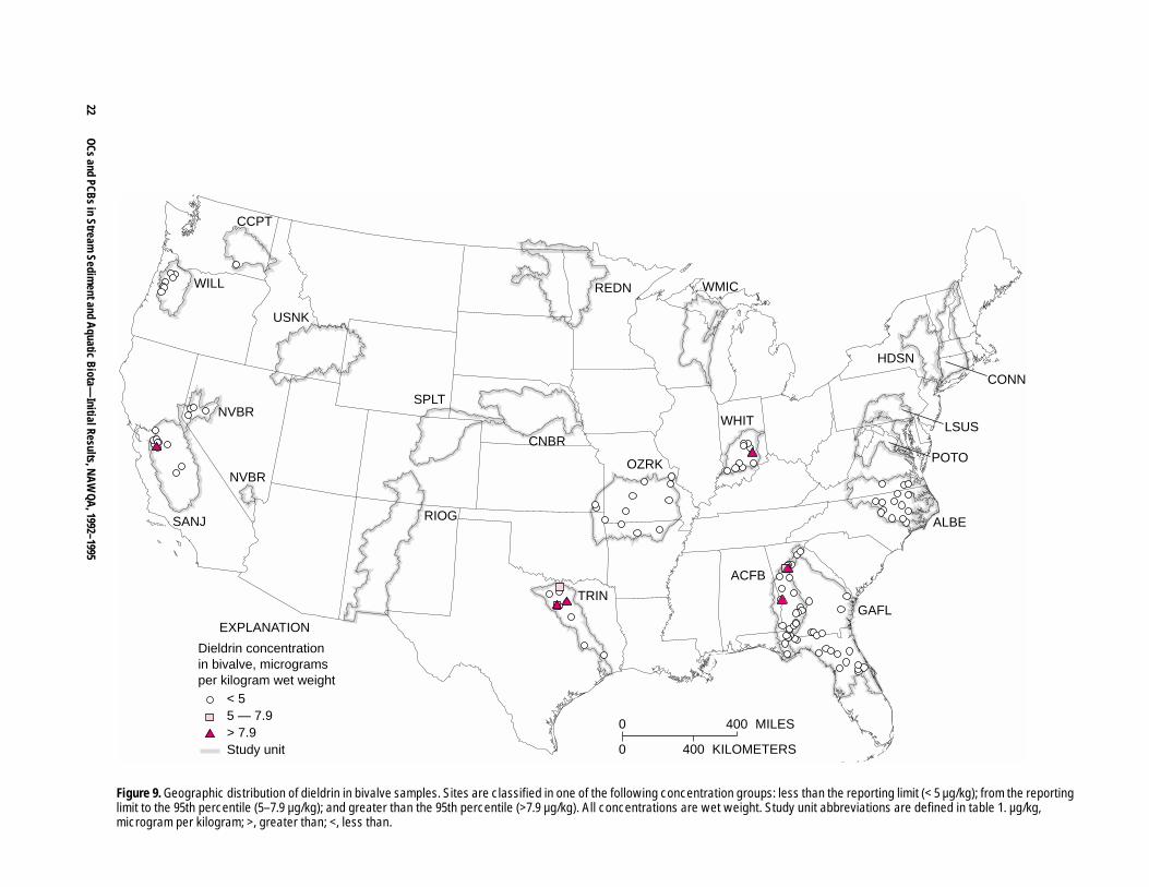
22O
Cs and PCBs in Stream
Sediment and A
quatic Biota—
Initial Results, NA
WQ
A, 1992–1995
WILL
CCPT
USNK
NVBR
NVBR
SANJ
TRIN
OZRK
CNBR
SPLT
REDN WMIC
WHIT
ACFB
GAFL
RIOG ALBE
POTO
LSUS
CONN
HDSN
< 55 — 7.9> 7.9Study unit
EXPLANATION
Dieldrin concentrationin bivalve, microgramsper kilogram wet weight
0 400 MILES
0 400 KILOMETERS
Figure 9. Geographic distribution of dieldrin in bivalve samples. Sites are classified in one of the following concentration groups: less than the reporting limit (< 5 µg/kg); from the reporting limit to the 95th percentile (5–7.9 µg/kg); and greater than the 95th percentile (>7.9 µg/kg). All concentrations are wet weight. Study unit abbreviations are defined in table 1. µg/kg, microgram per kilogram; >, greater than; <, less than.

National Overview 23
from urban areas (Arruda and others, 1987). This sug-gests that urban regions now may be the main source of chlordane to rivers, even in watersheds in Kansas, in which significant amounts of agricultural chlordane use have occurred in the past (Arruda and others, 1987).
To determine the relative distributions of the various chlordane compounds in the present study, percentages of the five components of total chlordane were quantified for all samples in which total chlor-dane was detected (that is, one or more component of total chlordane was detected). Values less than the reporting limit for any component were set equal to zero. The most abundant individual components in technical chlordane are cis- and trans-chlordane, whereas trans-nonachlor is the most persistent compo-nent (Schmitt and others, 1990). In the present study, the most abundant components of total chlordane detected were trans-chlordane in sediment and trans-nonachlor in biota (table 7). trans-Nonachlor com-prised a larger fraction of total chlordane in biota (mean percent composition of 52 percent in fish and 43 percent in bivalves) than in sediment (mean of 27 percent) or in technical chlordane (about 7 percent). cis-Nonachlor was detected in the present study at far lower percentages (mean percent composition of 4–10 percent in sediment, fish, and bivalves) than was present in technical chlordane (about 19 percent). Oxychlordane, a metabolite of chlordane not present in technical chlordane, also was observed in fish (mean percent composition of 7 percent), but not in bivalves, and at only trace levels in sediment (mean percent composition of 0.03 percent). Clearly, the composition of total chlordane in the environment has changed from the time chlordane was applied to the residues observed today.
The prevalence of trans-nonachlor in fish and bivalves in the present study is consistent with prior
studies. The NCBP found that the most abundant com-ponent of total chlordane was cis-chlordane prior to 1980, and trans-nonachlor in 1980 and afterwards (Schmitt and others, 1985, 1990). This shift in total chlordane composition was attributed to the weather-ing of chlordane constituents over time (Schmitt and others, 1990). The percent composition of total chlor-dane in fish that was observed in the present study is similar to that observed by Kawano and others (1988), who found the distribution in walleye, pollock, and chum salmon in the Arctic to be about 50 percent trans-nonachlor, 30 percent cis-chlordane, 10 percent trans-chlordane, 5 percent cis-nonachlor, and 5 per-cent oxychlordane.
The relative abundance of oxychlordane in fish compared with sediment suggests that it is accumulat-ing in fish as a transformation product of chlordane. Oxychlordane is a common metabolite of chlordane (Schwemmer and others, 1970; Street and Blau, 1972; Barnett and Dorough, 1974; Tashiro and Matsumura, 1977). Some fish species have been observed to degrade cis- and trans-chlordane into oxychlordane, albeit at a much slower rate than in mammals (Feroz and Khan, 1979; Khan and others, 1981). Oxychlor-dane is not expected to be preferentially bioaccumu-lated in fish compared with other chlordane isomers because the octanol-water partition coefficients of all of the major chlordane compounds (table 3) are very similar (Kawano and others, 1988). The absence of detectable oxychlordane in bivalves suggests either that bivalves do not degrade chlordane into oxychlor-dane or that oxychlordane, once formed in bivalves, is rapidly eliminated.
Total DDT
DDT was widely used in the United States as an insecticide for a variety of purposes in agricultural and urban areas, including the control of insects associated
Table 7. Mean percent composition of selected chlordane constituents and metabolites in sediment and aquatic biota from the National Water-Quality Assessment Program, 1992–1995, and in technical chlordane
[All values are in percent; ≈, approximately]
1Technical chlordane percentages are from Sovocool and others (1977) and Dearth and Hites (1991). Technical chlordane also includes other compounds, such as heptachlor and α-chlordene, that are not listed in the table.
Matrix cis-Chlordane trans-Chlordane cis-Nonachlor trans-Nonachlor Oxychlordane
Sediment 26 39 8.4 27 0.03
Fish 23 8.3 9.5 52 6.7
Bivalves 26 28 3.7 43 0
Technical chlordane1 19 24 ≈19 7 0

24O
Cs and PCBs in Stream
Sediment and A
quatic Biota—
Initial Results, NA
WQ
A, 1992–1995
WILL
CCPT
USNK
NVBR
NVBR
SANJ
TRIN
OZRK
CNBR
SPLT
REDN WMIC
WHIT
ACFB
GAFL
RIOG ALBE
POTO
LSUS
CONN
HDSN
0 400 MILES
0 400 KILOMETERS
< 11 — 6.6> 6.6 — 13> 13Study unit
EXPLANATION
Total chlordane concentrationin sediment, microgramsper kilogram dry weight
Figure 10. Geographic distribution of total chlordane in sediment samples. Sites are classified in one of the following concentration groups: less than the reporting limit (< 1 µg/kg); from the reporting limit to the 90th percentile (1–6.6 µg/kg); greater than the 90th percentile to the 95th percentile (>6.6–13 µg/kg); and greater than the 95th percentile (>13 µg/kg). All concentrations are dry weight. Study unit abbreviations are defined in table 1. µg/kg, microgram per kilogram; >, greater than; <, less than.

National O
verview25
WILL
CCPT
USNK
NVBR
NVBR
SANJ
TRIN
OZRK
CNBR
SPLT
REDN WMIC
WHIT
ACFB
GAFL
RIOG ALBE
POTO
LSUS
CONN
HDSN
0 400 MILES
0 400 KILOMETERS
EXPLANATION
Total chlordane concentrationin whole fish, microgramsper kilogram wet weight
< 55 — 16> 16 — 59> 59 — 85> 85Study unit
Figure 11. Geographic distribution of total chlordane in fish samples. Sites are classified in one of the following concentration groups: less than the reporting limit (< 5 µg/kg); from the reporting limit to the 75th percentile (5–16 µg/kg); greater than the 75th percentile to the 90th percentile (>16–59 µg/kg); greater than the 90th percentile to the 95th percentile (>59–85 µg/kg); and greater than the 95th percentile (>85 µg/kg). All concentrations are wet weight. Study unit abbreviations are defined in table 1. µg/kg, microgram per kilogram; >, greater than; <, less than.

26O
Cs and PCBs in Stream
Sediment and A
quatic Biota—
Initial Results, NA
WQ
A, 1992–1995
WILL
CCPT
USNK
NVBR
NVBR
SANJ
TRIN
OZRK
CNBR
SPLT
REDN WMIC
WHIT
ACFB
GAFL
RIOG ALBE
POTO
LSUS
CONN
HDSN
EXPLANATION
Total chlordane concentrationin bivalves, microgramsper kilogram wet weight
< 55 — 5.9> 5.9 — 24> 24Study unit
0 400 MILES
0 400 KILOMETERS
Figure 12. Geographic distribution of total chlordane in bivalve samples. Sites are classified in one of the following concentration groups: less than the reporting limit (< 5 µg/kg); from the reporting limit to the 90th percentile (5–5.9 µg/kg); greater than the 90th percentile to the 95th percentile (>5.9–24 µg/kg); and greater than the 95th percentile (>24 µg/kg). All concentrations are wet weight. Study unit abbreviations are defined in table 1. µg/kg, microgram per kilogram; >, greater than; <, less than.

National Overview 27
with public health issues (U.S. Environmental Protec-tion Agency, 1992b). Its use in the United States was terminated in 1972.
Total DDT concentrations in sediment (fig. 13) and fish (fig. 14) were highest in western Connecticut and Massachusetts, along the lower Hudson River, and in the western and northern regions of the Hudson River Basin. Bivalves were not sampled in this region of the country (fig. 15). For individual DDT compo-nents, the concentration distributions tracked the dis-tribution of total DDT, except that p,p′-DDT occurred less often and at lower concentrations in all three media than its metabolites p,p′-DDD and p,p′-DDE.
The geographical distribution in sediment of DDT and its major metabolites was generally in agree-ment with that found in previous studies. The PMN (1975–1992) found “hot spots,” defined as having median sediment concentrations greater than 7.5 µg/kg (dry weight) total DDT, and maximum concen-trations greater than 26 µg/kg (dry weight) total DDT, in the San Joaquin Valley, central Washington State, eastern Pennsylvania, Florida, and other scattered sites in the Southeast (Gilliom and others, 1985; Gilliom and Clifton, 1990). These levels found by the PMN were similar to the levels observed in the same areas in the present study. The occurrence of elevated total DDT levels in sediment in the Southeast is consistent with high historical agricultural use of DDT on cotton and other crops in this region (Gilliom and others, 1985). High sediment DDT concentrations also were found in the northwestern Pacific region, which is con-sistent with past DDT use in apple orchards of Wash-ington State (Rinella and others, 1992, 1993, 1996; Gilliom and Thelin, 1997).
Both the present study and the PMN found ele-vated DDT concentrations in sediment from the urban areas of the Hudson and lower Connecticut River basins. These elevated levels are consistent with the high nonfarm use and perhaps manufacturing of DDT in this industrialized region (Gilliom and others, 1985). The NS&T program, which measured total DDT in coastal and estuarine sediment, reported that total DDT in sediment was not significantly correlated with human population levels on a national scale because it was too highly associated with southern California (National Oceanic and Atmospheric Administration, 1991). Nonetheless, elsewhere in the country, high total DDT concentrations in estuarine sediment tended to be associated with high population densities (Nowell and others, 1999).
The total DDT concentrations in fish detected in the present study are consistent with the results of pre-vious studies, the NCBP (Schmitt and others, 1981, 1983, 1985, 1990) and the NSCRF (U.S. Environmen-tal Protection Agency, 1992a,b). Elevated total DDT concentrations in fish were found in the Hudson, Con-necticut, lower Susquehanna, Platte, Snake, Columbia, and lower Willamette river basins (fig. 14). Elevated concentrations of DDT and its metabolites, particu-larly DDE, were also observed in fish in the upper Rio Grande River Basin in New Mexico. These results agree with those of prior studies, which found high occurrences of DDE in fish and other wildlife in this area (Clark and Krynitsky, 1983; White and Krynitsky, 1986).
The predominant DDT component in all sam-pling media was p,p′-DDE. The mean percent compo-sition of total DDT in sediment and biota samples (shown in table 8) was calculated in a similar manner as was done for total chlordane. In the present study, the calculation of the percent composition of total DDT is complicated by analytical difficulties with thermal degradation of DDT to DDD inside the GC injection port for some samples (Leiker and others, 1995; Foreman and Gates, 1997). As a consequence, the relative abundance of DDT and DDD should be considered lower and upper bounds, respectively. Although the largest fraction of total DDT in all three media was composed of p,p′-DDE, the relative abun-dance of p,p′-DDE was higher in both fish (mean per-cent composition of 84.5 percent) and bivalves (91.7 percent) than in sediment (55.9 percent). In contrast, sediment contained a higher fraction of p,p′-DDD (mean percent composition of 20.2 percent) than did biota (9.6 percent for fish and 2.1 percent for bivalves).
DDT was marketed primarily as technical DDT, which contained 77.1 percent p,p′-DDT, 14.9 percent o,p′-DDT, 4.0 percent p,p′-DDE, 0.1 percent o,p′-DDE, and 3.5 percent unidentified products (table 8) (World Health Organization, 1989). The mean per-cent composition of total DDT observed in all media in the present study is clearly different from that in technical DDT, as shown in table 8. DDT is metabo-lized into DDE aerobically via dehydrochlorination (Brooks, 1974) and into DDD anaerobically via reduc-tive dechlorination (Fries, 1972). In previous studies, the NCBP computed the percent composition of total DDT (defined as the sum of p,p′ isomers of DDD, DDE, and DDT) in whole freshwater fish. The mean percent composition of p,p′ isomers in fish changed

28O
Cs and PCBs in Stream
Sediment and A
quatic Biota—
Initial Results, NA
WQ
A, 1992–1995
WILL
CCPT
USNK
NVBR
NVBR
SANJ
TRIN
OZRK
CNBR
SPLT
REDN WMIC
WHIT
ACFB
GAFL
RIOG ALBE
POTO
LSUS
CONN
HDSN
0 400 MILES
0 400 KILOMETERS
EXPLANATION
Total DDT concentrationin sediment, microgramsper kilogram dry weight
< 11 — 3.9> 3.9 — 19> 19 — 44> 44Study unit
Figure 13. Geographic distribution of total DDT in sediment samples. Sites are classified in one of the following concentration groups: less than the reporting limit (< 1 µg/kg); from the reporting limit to the 75th percentile (1–3.9 µg/kg); greater than the 75th percentile to the 90th percentile (>3.9–19 µg/kg); greater than the 90th percentile to the 95th percentile (>19–44 µg/kg); and greater than the 95th percentile (>44 µg/kg). All concentrations are dry weight. Study unit abbreviations are defined in table 1. µg/kg, microgram per kilogram; >, greater than; <, less than.

National O
verview29
WILL
CCPT
USNK
NVBR
NVBR
SANJ
TRIN
OZRK
CNBR
SPLT
REDN WMIC
WHIT
ACFB
GAFL
RIOG ALBE
POTO
LSUS
CONN
HDSN
< 55 — 31> 31 — 100> 100 — 254> 254 — 439> 439Study unit
EXPLANATION
Total DDT concentrationin whole fish, microgramsper kilogram wet weight
0 400 MILES
0 400 KILOMETERS
Figure 14. Geographic distribution of total DDT in fish samples. Sites are classified in one of the following concentration groups: less than the reporting limit (< 5 µg/kg); from the reporting limit to the 50th percentile (5–31 µg/kg); greater than the 50th percentile to the 75th percentile (>31–100 µg/kg); greater than the 75th percentile to the 90th percentile (>100–254 µg/kg); greater than the 90th percentile to the 95th percentile (>254–439 µg/kg); and greater than the 95th percentile (>439 µg/kg). All concentrations are wet weight. Study unit abbreviations are defined in table 1. µg/kg, microgram per kilogram; >, greater than; <, less than.

30O
Cs and PCBs in Stream
Sediment and A
quatic Biota—
Initial Results, NA
WQ
A, 1992–1995
WILL
CCPT
USNK
NVBR
NVBR
SANJ
TRIN
OZRK
CNBR
SPLT
REDN WMIC
WHIT
ACFB
GAFL
RIOG ALBE
POTO
LSUS
CONN
HDSN
< 55 — 5.3> 5.3 — 16> 16 — 25> 25Study unit
EXPLANATION
Total DDT concentrationin bivalves, microgramsper kilogram wet weight
0 400 MILES
0 400 KILOMETERS
Figure 15. Geographic distribution of total DDT in bivalve samples. Sites are classified in one of the following concentration groups: less than the reporting limit (< 5 µg/kg); from the reporting limit to the 75th percentile (5–5.3 µg/kg); greater than the 75th percentile to the 90th percentile (>5.3–16 µg/kg); greater than the 90th percentile to the 95th percentile (>16–25 µg/kg); and greater than the 95th percentile (>25 µg/kg). All concentrations are wet weight. Study unit abbreviations are defined in table 1. µg/kg, microgram per kilogram; >, greater than; <, less than.

National Overview 31
little from 1976 to 1981, consisting of about 70 per-cent p,p′-DDE, 20 percent p,p′-DDD, and 10 percent p,p′-DDT; however, the percentage of p,p′-DDE increased in 1984 to 73 percent (Schmitt and others, 1990) and in 1986 to 78 percent (U.S. Fish and Wild-life Service, 1992). The predominance of p,p′-DDE found in fish in the present study (84.5 percent of total DDT; table 8) may reflect a continued trend toward a relatively higher proportion of p,p′-DDE.
Laboratory and field-plot estimates of soil half-lives for DDT range from 2 to 16 years (Ware and oth-ers, 1971, 1974, 1978; Lichtenstein and others, 1971; Howard and others, 1991). However, more recent field monitoring studies (for example, Mischke and others, 1985) indicate that DDT half-lives in soil can be on the order of 15 years or longer. Therefore, soils to which DDT was applied before its ban in the early 1970s could retain much of their DDT burden for several decades (Rinella and others, 1992, 1993, 1996). In a statewide survey of soils in California (Mischke and others, 1985), soils historically treated with DDT had a mean (parent DDT/total DDT) ratio of 49 percent, which is higher than is generally found in sediment. DDT appears to break down more quickly once it enters a river or other waterway (Agee, 1986). Sedi-ment or biota samples that contain a high (DDT/ total DDT) ratio probably indicate that the residues recently entered the hydrologic system (Aguillar, 1984; Agee, 1986), such as by erosion of DDT-contaminated soil (Johnson and others, 1988; Rinella, 1993; Nowell and others, 1999). NAWQA sites with the highest p,p′-DDT proportions (larger than 2 standard deviations (σ) above mean, that is, the 95 percent confidence interval) were scattered in southern Pennsylvania and in the Connecticut and the Willamette river valleys. These sites were generally in or near urban areas, sug-gesting recent urban inputs of DDT to the hydrologic system.
The ratio of o,p′ isomers to total DDT is also useful for determining industrial (noninsecticidal) sources of DDT. Technical DDT, as applied for insec-ticidal use, contained about 71 percent p,p′-DDT and 14.9 percent o,p′-DDT (World Health Organization, 1989). Waste products from the manufacture of techni-cal DDT are generally enriched in o,p′-DDT relative to the active ingredient p,p′-DDT, so an excess (greater than 20 percent) of o,p′ isomers suggests a noninsecti-cidal source (Nowell and others, 1999). In the present study, the average ratio of o,p′ isomers to total DDT (with total DDT defined as the sum of o,p′ and p,p′ isomers) is 5.6 percent in sediment, 1.3 percent in fish, and 0.4 percent in bivalves. In sediment, there were 12 sites at which the ratio of o,p′ to total DDT exceeded 20 percent. For fish, there were two sites. Most of the samples with a high ratio of o,p′ isomers to total DDT were located in or near urban areas in Pennsylvania, Connecticut, and New York. The sites near Hartford and New York City also had a higher than average pro-portion of DDT to total DDT (with a mean of 66.4 per-cent p,p′-DDT), which, in conjunction with the high ratio of o,p′ isomers to total DDT, suggests recent addition of soil contaminated with DDT from indus-trial sources to these hydrologic systems.
Total PCBs
PCBs are a mixture of compounds formed by the chlorination of biphenyl. There are 209 different PCB compounds (termed “congeners”) that have dif-ferent chlorine substitution patterns. In the United States, mixtures of various PCB congeners were for-mulated for commercial use under the trade name Aro-clor on the basis of their percent chlorine content. For example, Aroclor 1254 has an average chlorine con-tent of 54 percent by weight (U.S. Environmental Pro-tection Agency, 1995). PCBs were used as dielectric fluids in transformers, capacitors and electromagnets,
Table 8. Mean percent composition of o,p′- and p,p′-DDT and their primary metabolites in sediment and aquatic biota from the National Water-Quality Assessment Program, 1992–1995, and in technical DDT
[All values are in percent]
1Technical DDT percentages are from the World Health Organization (1989). In addition to the compounds listed above, 3.5 percent of the total was listed as unidentified products.
Matrix o,p′-DDD p,p′-DDD o,p′-DDE p,p′-DDE o,p′-DDT p,p′-DDT
Sediment 4.6 20.2 0.1 55.9 0.9 18.3
Fish 0.6 9.6 0.4 84.5 0.3 4.6
Bivalves 0.1 2.1 0.1 91.7 0.2 5.8
Technical DDT1 0.1 0.3 0.1 4 14.9 77.1
32 OCs and PCBs in Stream Sediment and Aquatic Biota—Initial Results, NAWQA, 1992–1995
and as plasticizers, lubricants, and ink carriers prior to the early 1970s (Erickson, 1997). These uses are gen-erally associated with industrial processes in urban settings. Production and use of PCBs in the United States was banned by the EPA in 1979 (U.S. Environ-mental Protection Agency, 1995).
The comparison of the geographical distribution of PCBs from the present study with those from prior studies is complicated by analytical considerations. Whereas early studies measured PCBs using packed-column gas chromatography and quantified total PCBs as the sum of one or more Aroclor mixtures using regression techniques (Schmitt and others, 1981), later studies employed capillary-column gas chromatogra-phy to resolve individual congeners (Mullin and oth-ers, 1984) and reported total PCBs either as the sum of the congeners (which varied by study and by analyti-cal method) or as Aroclor mixtures in keeping with prior studies (Schmitt and others, 1985, 1990). In the present study, the total PCB concentration was deter-mined by summing the peak areas for 10 to 15 repre-sentative congeners relative to a calibration standard consisting of a mixture of Aroclors (Leiker and others, 1995). Because of differences in how different studies computed total PCB concentrations, comparison between studies of PCB concentrations and distribu-tions should be regarded with caution. Despite the complications imposed by analytical differences, the geographic distribution of PCBs in the present study appears to be similar to those found in prior studies.
Total PCB concentrations were highest in the northeastern part of the United States for both sedi-ment (fig. 16) and aquatic biota (figs. 17 and 18). Total PCB concentrations in whole fish (fig. 17) at many sites in the Hudson and Connecticut river basins were about 1,000 µg/kg wet weight with a maximum con-centration of 72,000 µg/kg wet weight in the Housa-tonic River at Lenox, Mass. A site near Pleasureville, Penn., in the lower Susquehanna River Basin had a PCB concentration of 1,500 µg/kg wet weight in fish. Elevated PCB concentrations also were observed in the Willamette River near Portland, Oreg., where the levels were generally 400–1,200 µg/kg wet weight. These observations are in agreement with the results of the NCBP (Schmitt and others, 1981, 1983, 1985, 1990) and the NSCRF (U.S. Environmental Protection Agency, 1992a,b), both of which studies found ele-vated PCB concentrations in fish in the Hudson, Con-necticut, lower Susquehanna, Platte, and lower Willamette river basins.
In addition to the areas mentioned above, ele-vated PCB concentrations in sediment (200–700 µg/kg dry weight) were measured in the urban areas of east-ern Wisconsin (Green Bay, Sheboygan, and Milwau-kee); no fish were collected at these sites. The presence of elevated levels of PCBs in the sediment of the western Lake Michigan tributaries is in agreement with reports that this area is a major source of PCBs to the Great Lakes region (Swackhamer and Armstrong, 1988; Hermanson and others, 1991; Manchester, 1993; Golden, 1994).
Relations Among Sampling Media
Bed sediment and aquatic biota (fish and bivalves) were sampled in the NAWQA Program because these sampling media accumulate hydropho-bic compounds and, thus, each can provide a sensitive means of determining whether these compounds are present in a hydrologic system. Together, sediment and aquatic biota comprise dual lines of evidence for con-tamination of a hydrologic system. Each sampling medium, taken alone, has its advantages and disadvan-tages. Sediment sampled from depositional areas rep-resents exposure at a given site, yet it also integrates contaminants that have accumulated at that site over an unknown period of time. Fish are excellent accu-mulators of hydrophobic contaminants, but they also are mobile, so their contaminant burden may reflect exposure in other parts of the hydrologic system than at the site sampled. Also, a national-scale study will need to sample multiple fish species because no single fish species will be available at all sampling sites. Interspecies differences, as well as differences in life stage and physiological condition, may complicate interpretation of fish contaminant data. Finally, bivalves, although stationary, are not found in all parts of the United States and generally have lower lipid content and OC contaminant concentrations than many fish species.
In this section, comparisons are made between OC concentrations detected in sediment, fish, and bivalves in the present study. Similarities and differ-ences between OC concentrations in these sampling media provide dual lines of evidence regarding con-tamination at a given site, as well as general informa-tion about the usefulness of these sampling media as OC accumulators.

National O
verview33
WILL
CCPT
USNK
NVBR
NVBR
SANJ
TRIN
OZRK
CNBR
SPLT
REDN WMIC
WHIT
ACFB
GAFL
RIOG ALBE
POTO
LSUS
CONN
HDSN
< 100100 — 146> 146Study unit
EXPLANATION
Total PCB concentrationin sediment, microgramsper kilogram dry weight
0 400 MILES
0 400 KILOMETERS
Figure 16. Geographic distribution of total PCBs in sediment samples. Sites are classified in one of the following concentration groups: less than the reporting limit (< 100 µg/kg); from the reporting limit to the 95th percentile (100–146 µg/kg); and greater than the 95th percentile (>146 µg/kg). All concentrations are dry weight. Study unit abbreviations are defined in table 1. PCB, polychlorinated biphenyl. µg/kg, microgram per kilogram; >, greater than; <, less than.

34O
Cs and PCBs in Stream
Sediment and A
quatic Biota—
Initial Results, NA
WQ
A, 1992–1995
WILL
CCPT
USNK
NVBR
NVBR
SANJ
TRIN
OZRK
CNBR
SPLT
REDN WMIC
WHIT
ACFB
GAFL
RIOG ALBE
POTO
LSUS
CONN
HDSN
< 5050 — 150> 150 — 646> 646 — 1,400> 1,400Study unit
EXPLANATION
Total PCB concentrationin whole fish, microgramsper kilogram wet weight
0 400 MILES
0 400 KILOMETERS
Figure 17. Geographic distribution of total PCBs in fish samples. Sites are classified in one of the following concentration groups: less than the reporting limit (< 50 µg/kg); from the reporting limit to the 75th percentile (50–150 µg/kg); greater than the 75th percentile to the 90th percentile (>150–646 µg/kg); greater than the 90th percentile to the 95th percentile (>646–1,400 µg/kg); and greater than the 95th percentile (>1,400 µg/kg). All concentrations are wet weight. Study unit abbreviations are defined in table 1. PCB, polychlorinated biphenyl. µg/kg, microgram per kilogram; >, greater than; <, less than.

National O
verview35
WILL
CCPT
USNK
NVBR
NVBR
SANJ
TRIN
OZRK
CNBR
SPLT
REDN WMIC
WHIT
ACFB
GAFL
RIOG ALBE
POTO
LSUS
CONN
HDSN
< 5050 — 83> 83Study unit
EXPLANATION
Total PCB concentrationin bivalves, microgramsper kilogram wet weight
0 400 MILES
0 400 KILOMETERS
Figure 18. Geographic distribution of total PCBs in bivalve samples. Sites are classified in one of the following concentration groups: less than the reporting limit (< 50 µg/kg); from the reporting limit to the 95th percentile (50–83 µg/kg); and greater than the 95th percentile (>83 µg/kg). All concentrations are wet weight. Study unit abbreviations are defined in table 1. PCB, polychlorinated biphenyl. µg/kg, microgram per kilogram; >, greater than; <, less than.

36 OCs and PCBs in Stream Sediment and Aquatic Biota—Initial Results, NAWQA, 1992–1995
Sediment Versus Fish
In this study, there are 3,209 measurements of individual target analytes in paired sediment–fish sam-ples. Of these, only 184 measurements of individual target analytes were quantified above the reporting limits in both media. This data set, which will be used for comparisons in this section, consists predomi-nantly of DDT and its metabolites, in particular p,p′-DDE, as well as some chlordane components, dield-rin, and total PCBs (listed in table 9). Heptachlor epoxide and dacthal had one paired measurement each.
Although there does appear to be some relation between concentrations in sediment and fish (r2 = 0.43), a great deal of variability exists in this relation-ship (fig. 19). Normalizing the sediment and fish con-centrations to sediment organic carbon and lipid content, respectively, results in a slightly improved relation (r2 = 0.45), but does not reduce the scatter in the data to any great extent (fig. 19). The exclusion of the highest concentration, a known PCB contamina-tion site near Pittsfield, Mass., which appears to drive both regressions, does decrease the r2 value for both nonnormalized (r2 = 0.35) and normalized (r2 = 0.37) relations, but does not unduly change the distribution and cannot be considered an outlier. There is often, but not always, a stronger relation between paired site sediment and fish concentrations when individual ana-lytes are compared (table 9). Usually, but not always, normalization increases the r2 value somewhat. How-ever, there is still a great deal of variability for individ-ual analytes. Moreover, for those compounds for which the r2 is relatively high (and variability low), the data set tends to be small. As an example, the r2 value for total PCBs is 0.87 for the normalized regres-sion and 0.55 for the non-normalized regression, but the sample size for total PCBs (seven paired measure-ments) is small. Although there is a relation between high sediment concentrations and high fish concentra-tions at a site, other factors besides sediment organic carbon and lipid normalization, such as species, sex, age, and diet, contribute to the variability between the concentrations in the two media.
Fish Versus Bivalves
As discussed previously, most of the aquatic biota collected for tissue analysis in the present study
were fish because bivalves were found only in some parts of the United States. In addition, most of the OC concentrations in bivalves were below the reporting limit, although some of these same OCs were detected quite frequently in fish. The following analysis is based only on sites at which both fish and bivalves were collected on the same day. Of the 168 paired measurements of fish and bivalves in the present study, only seven of these measurements had concentrations above the reporting limit in both media. These seven measurements came from three sites: two were p,p′-DDE measurements, and the remaining five were of cis-chlordane, trans-chlordane, cis-nonachlor, trans-nonachlor, and dieldrin. As shown in figure 20, there is a much stronger relation for the lipid normal-ized concentrations (r2 = 0.94) than the wet-weight concentrations (r2 = 0.094) for these seven paired mea-surements, suggesting that differences in lipid levels account for much of the difference in concentration between the two media. However, the extremely lim-ited number of detections in paired fish–bivalve sam-ples limits the conclusions about the relation between these two media.
Table 9. Coefficients of determination for linear regressions between concentrations in paired sediment–fish samples
[Coefficients of determination (r2) are shown for non-normalized concentrations in sediment and fish (micro-grams per kilogram dry weight and micrograms per kilo-gram wet weight, respectively) and for sediment organic carbon-normalized concentrations in sediment (micrograms per kilogram of sediment organic carbon) and lipid-normal-ized concentrations in fish (micrograms per kilogram of lipid). PCB, polychlorinated biphenyl]
Target
analyte
Number
of paired
measurements
Coefficients of
determination
(non-normal-
ized)
Coefficients of
determination
(normalized)
All analytes 184 0.43 0.45
Dieldrin 16 0.31 0.58
Total chlordane 52 0.25 0.06
cis-Chlordane 16 0.35 0.38
trans-Chlordane 12 0.42 0.16
cis-Nonachlor 7 0.31 0.13
trans-Nonachlor 17 0.4 0.12
Total DDT 107 0.16 0.23
p,p′-DDD 24 0.57 0.6
p,p′-DDE 58 0.31 0.56
p,p′-DDT 18 0.15 0.37
Total PCBs 7 0.55 0.87

National Overview 37
0
1
2
3
4
5
0 1 2 3 4 5
7
0
1
2
3
4
5
6
0 1 2 3 4 5 6 7
B.
A.Lo
g fis
h co
ncen
trat
ion,
in m
icro
gram
s pe
r ki
logr
am (
wet
wei
ght)
Log
fish
conc
entr
atio
n, in
mic
rogr
ams
per
kilo
gram
of l
ipid
y = 0.72x + 1.12r2 = 0.43
y = 0.71x + 1.21r2 = 0.45
Log sediment concentration, in micrograms per kilogram (dry weight)
Log sediment concentration, in micrograms per kilogram of sediment organic carbon
Figure 19. Relation between the concentrations of organochlorine analytes in paired sediment–fish samples. A, Logarithms of non-normalized sediment and fish concentrations. B, Logarithms of organic-carbon-normalized sediment concentration and lipid-normalized fish concentration. Each point represents the concentrations of a single analyte in the two media. Also shown are the least squares regression line (black line) and equation and the line denoting a 1:1 relation between sediment and fish concentrations (gray line). r, correlation coefficient.

38 OCs and PCBs in Stream Sediment and Aquatic Biota—Initial Results, NAWQA, 1992–1995
0
5
10
15
20
0 10 20 30 40 50
0
400
800
1,200
1,600
2,000
0 200 400 600 800 1,000 1,200 1,400
y = 0.10x + 8.73r2 = 0.094
y = 1.22x + 185.43r2 = 0.94
Fish concentration, in micrograms per kilogram (wet weight)
Fish concentration, in micrograms per kilogram of lipid
Biv
alve
con
cent
ratio
n, in
mic
rogr
ams
per
kilo
gram
(w
et w
eigh
t)
Biv
alve
con
cent
ratio
n, in
mic
rogr
ams
per
kilo
gram
of l
ipid
B.
A.
Figure 20. Relation between the concentrations of organochlorine analytes in paired bivalve–fish samples. A, Logarithms of non-normalized bivalve and fish concentrations. B, Logarithms of lipid-normalized bivalve and fish concentrations. Each point represents the concentrations of a single analyte in the two media. Also shown are the least squares regression line (black line) and equation and the line denoting a 1:1 relation between bivalve and fish concentrations (gray line). r, correlation coefficient.

National Overview 39
Effects of Reporting Limit Censoring on the Frequency of Detection
Because the reporting limits vary among the target analytes in bed sediment and tissue, a censoring analysis was performed to calculate detection frequen-cies at a series of raised reporting limits. This was done to determine whether a common reporting limit was feasible, at least for the most frequently detected analytes. Because detection frequency varies as a function of the reporting limit, detection frequencies among individual target analytes should be compared at a uniform reporting limit, if possible. In sediment, reporting limits for most analytes varied from 1 to 5 µg/kg dry weight. The exceptions had substantially high reporting limits: hexachlorobenzene and pen-tachloroanisole (reporting limits of 50 µg/kg dry weight), total PCBs (100 µg/kg dry weight), and tox-aphene (200 µg/kg dry weight). In fish, all analytes had a common reporting limit (5 µg/kg wet weight) except total PCBs (50 µg/kg wet weight).
Because of the distributions of these reporting limits, two different censoring scenarios were investi-gated. In scenario A, censoring limits from 1 to 5 µg/kg dry weight were applied to sediment data only from sites that had nonmissing data for the most com-monly detected pesticides: total DDT, total chlordane, and dieldrin. Sites at which data for one or more of these compounds were missing were not used in this scenario to avoid biasing detection frequencies. The detection frequencies for this subset of the sediment data are listed in table 10 at censoring limits from 1 to 5 µg/kg dry weight. These detection frequencies are different from those listed in table 3 for the same reporting limits because the current scenario uses only a subset of the sites.
Applying a common censoring level to all target analytes reduces the amount of sediment data for many of the analytes (table 10). Censoring the data at 2 µg/kg dry weight—the reporting level of o,p′-DDT and p,p′-DDT—would put most compounds (all except dacthal, hexachlorobenzene, o,p′- and p,p′-methoxychlor, cis- and trans-permethrin, total PCBs, pentachloroanisole, and toxaphene) at a uni-form reporting limit. However, this would reduce the detection frequencies of several compounds. For example, detection frequencies would be reduced from 33 to 24 percent for p,p′-DDE and from 11 to 5 per-cent for dieldrin. If the data were censored at 5 µg/kg dry weight, which would bring all compounds except
hexachlorobenzene, total PCBs, pentachloroanisole, and toxaphene to a common reporting limit, the detec-tion frequencies for p,p′-DDE and dieldrin would be further reduced to 11 and 1 percent, respectively. Although applying various censoring levels to the data lowers the observed detection frequencies, it does not alter which analytes were most commonly detected in sediment. Excluding PCBs and the other three ana-lytes with very high reporting limits, detection fre-quencies in sediment consistently follow the same order: p,p′-DDE has the highest detection frequency, followed by p,p′-DDD and p,p′-DDT, followed by trans-chlordane, trans-nonachlor, cis-chlordane, and dieldrin.
In fish, all compounds except total PCBs have a common reporting limit (5 µg/kg wet weight). There-fore, no low-limit censoring is necessary for fish data. Excluding total PCBs, the order of detection frequen-cies in fish is as follows: p,p′-DDE has the highest detection frequency, followed by p,p′-DDD, followed by trans-nonachlor, followed by p,p-DDT and dield-rin, followed by cis-chlordane.
In scenario B, the analytes with very high reporting limits in sediments (which were not exam-ined in the first scenario) are accounted for by apply-ing censoring limits from 2 to 200 µg/kg dry weight. Only data for sites with nonmissing data for total PCBs, hexachlorobenzene, pentachloroanisole (the principal industrial contaminants), and p,p′-DDE (the most commonly detected pesticide analyte) were used to avoid biasing detection frequencies. In practice, only PCBs and p,p′-DDE were used in selecting this subset because the other two analytes were detected so rarely (fig. 3). Censoring data at such high reporting limits is bound to reduce detection frequencies of the pesticides that originally had much lower reporting limits. However, the high-limit censoring in scenario B does permit comparison of detection frequencies for industrial contaminants (especially total PCBs) with those for the most commonly detected pesticides (DDT compounds, chlordane components, and dield-rin). Tables 11 and 12 summarize the detection fre-quencies from scenario B for bed sediment and fish, respectively. The detection frequencies are slightly dif-ferent in this scenario than in scenario A (table 10) because of the larger data subset produced by a less restrictive selection rule.
Applying a high censoring limit drastically reduces the detection frequencies for analytes with lower reporting limits in both sediment (table 11) and

40 OCs and PCBs in Stream Sediment and Aquatic Biota—Initial Results, NAWQA, 1992–1995
fish (table 12). However, the comparison of detection frequencies for individual analytes at a common reporting limit indicates the following. First, total PCBs is detected more frequently than p,p′-DDE and the other pesticides when detection frequencies are censored at a common reporting limit (50 µg/kg wet weight in fish and 100 µg/kg dry weight in sediment). Second, toxaphene has a comparable detection fre-
quency to p,p′-DDT, dieldrin, and o,p′-DDD in sedi-ment, and to p,p′-DDE in fish when data are censored at 200 µg/kg dry weight and wet weight, respectively. This does not mean that the concentration distributions of total PCBs and toxaphene would be comparable to those of the DDT compounds, for example, if the reporting limits for total PCBs and toxaphene had been lower. Figure 4 suggests that the concentration
Table 10. Detection frequencies in sediment, 1992–1995, at censoring levels from 1 to 5 µg/kg dry weight
[See text for details. There were 309 total sites. Compounds are listed in order of detection frequency in fish shown in table 5. PCB, polychlorinated biphenyl; µg/kg, microgram per kilogram; —, not applicable because censoring level is less than origi-nal reporting limit for that analyte]
Target analyte
Censoring level
(µg/kg, dry weight): 1 2 3 4 5
Frequency of detection (in percent)
p,p′-DDE 33.3 24.3 17.8 12.6 11.6
Total PCBs — — — — —
p,p′-DDD 20.4 15.5 10 8.4 7.1
trans-Nonachlor 12.9 7.4 2.9 1.6 1.3
p,p′-DDT — 15.9 10 7.8 6.5
Dieldrin 10.7 5.2 3.9 1.6 1.3
cis-Chlordane 12.3 7.2 3.6 1.9 1.6
cis-Nonachlor 7.4 2.9 1 1 0
trans-Chlordane 13.6 9 4.8 2.9 1.9
Oxychlordane 0 0 0 0 0
o,p′-DDD 9.1 4.2 3.9 2.6 1.9
Pentachloroanisole — — — — —
Hexachlorobenzene — — — — —
o,p′-DDT — 3.2 2.9 1.6 1
Heptachlor epoxide 1.3 0.3 0.3 0.3 0
o,p′-DDE 1.6 1 0.6 0.6 0.3
γ-HCH 1.3 0.6 0.3 0.3 0.3
Dacthal — — — — 1.6
Endrin — 0 0 0 0
α-HCH 0 0 0 0 0
Toxaphene — — — — —
Aldrin 0.6 0.6 0.3 0 0
Mirex 1.3 1 0.3 0.3 0
p,p′-Methoxychlor — — — — 0.7
o,p′-Methoxychlor — — — — 0
β-HCH 0.6 0 0 0 0
Heptachlor 0 0 0 0 0
Endosulfan 2.3 1.3 1 1 0.6
cis-Permethrin — — — — 1.4
trans-Permethrin — — — — 1.1
Chloroneb — — — — 0
Isodrin 0 0 0 0 0

National Overview 41
distribution of total PCBs may be different from that of total DDT, at least in fish and bivalves (note the converging cumulative frequency curves in fig. 4).
In summary, the majority of detections for pesti-cides in sediment are at low concentrations, generally below 5 µg/kg dry weight. Consequently, censoring of the sediment data at a common reporting limit would result in the conversion of a substantial portion of the detectable concentrations for pesticides to nondetec-tions. Censoring of the fish data set is not necessary
because almost all pesticides have a common reporting limit (5 µg/kg wet weight). However, detection fre-quencies for a few analytes (namely, total PCBs, tox-aphene, and, in sediment, hexachlorobenzene and pentachloroanisole) always should be considered in the light of their very high reporting limits. In the remainder of this report, no common censoring levels will be applied, except in assessment of concentration trends over time and whenever results for different analytes are compared.
Table 11. Detection frequencies in sediment, 1992–1995, at censoring levels from 1 to 200 µg/kg dry weight
[See text for details. There were 217 total sites. Compounds are listed in order of detection frequency in fish shown in table 5. PCB, polychlorinated biphenyl; µg/kg, microgram per kilogram; —, not applicable because censoring level is less than origi-nal reporting limit for that analyte]
Target analyte
Censoring level
(µg/kg, dry weight):1 2 5 50 100 200
Frequency of detection (in percent)
p,p′-DDE 38.9 26.9 13 1.7 0.7 0.2
Total PCBs — — — — 4.8 2.9
p,p′-DDD 25 18.7 8.9 0.9 0.3 0
trans-Nonachlor 15.6 9.9 2.5 0 0 0
p,p′-DDT — 18.8 8.4 1.1 0.9 0
Dieldrin 14 8.1 2.2 0 0 0
cis-Chlordane 15.5 9.1 3 0 0 0
cis-Nonachlor 8.9 4.2 0.7 0 0 0
trans-Chlordane 16.7 10.5 3.4 0 0 0
Oxychlordane 0.2 0 0 0 0 0
o,p′-DDD 11 5.2 2.3 0.3 0.3 0
Pentachloroanisole — — — 0 0 0
Hexachlorobenzene — — — 0 0 0
o,p′-DDT — 3.1 1.1 0 0 0
Heptachlor epoxide 1.2 0.2 0 0 0 0
o,p′-DDE 2 0.8 0.2 0 0 0
γ-HCH 1 0.5 0.2 0 0 0
Dacthal — — 1.5 0 0 0
Endrin — 0 0 0 0 0
α-HCH 0 0 0 0 0 0
Toxaphene — — — — — 0.2
Aldrin 0.5 0.5 0 0 0 0
Mirex 2 1 0 0 0 0
p,p′-Methoxychlor — — 0.8 0.3 0 0
o,p′-Methoxychlor — — 0 0 0 0
β-HCH 0.5 0 0 0 0 0
Heptachlor 0.2 0 0 0 0 0
Endosulfan 2.5 1.5 0.7 0 0 0
cis-Permethrin — — 1.2 0 0 0
trans-Permethrin — — 0.9 0 0 0

42 OCs and PCBs in Stream Sediment and Aquatic Biota—Initial Results, NAWQA, 1992–1995
EFFECT OF LAND USE ON ORGANOCHLORINE CONCENTRATIONS
The terrestrial environment has a strong influ-ence on the water quality of adjacent hydrologic sys-tems. Both natural and anthropogenic characteristics of the terrestrial environment are important. For exam-ple, concentrations of major chemical constituents (such as sulfate, calcium, and pH) in a hydrologic sys-tem are influenced by geology, and the concentration of suspended sediment is influenced by soil character-istics, topography, and land cover (Nowell and others, 1999). The application of most pesticides is directly
related to land use. Therefore, land-use activities such as row crop agriculture, pasture, forestry, industry, and urbanization can result in pesticide inputs to adjacent water bodies.
Historically, the OC insecticides have been applied in agriculture; in urban and residential settings for control of public-health insects, termites, and nui-sance insects; and in forestry. OC insecticides were used in urban and residential areas more recently (through the late 1980s) than in agricultural applica-tions (which were banned or restricted during the 1970s for most OC insecticides). Moreover, the avail-able quantitative data on nonagricultural pesticide use
Table 12. Detection frequencies in whole fish, 1992–1995, at censoring levels from 5 to 200 µg/kg wet weight
[See text for details. There were 232 total sites. Compounds are listed in order of detection frequency in fish shown in table 5. PCB, poly-chlorinated biphenyl; µg/kg, microgram per kilogram; —, not applicable because censoring level is less than original reporting limit for that analyte]
Target analyte
Censoring level
(µg/kg, dry weight):5 6 7 8 9 10 50 100 200
Frequency of detection (in percent)
p,p′-DDE 79.7 77.2 74.6 72.8 71.6 70.3 36.2 21.6 8.6
Total PCBs — — — — — — 44.4 29.3 19.0
p,p′-DDD 42.2 39.9 37.2 33.6 33.2 31.8 4 2.2 0.9
trans-Nonachlor 33.5 30.9 29.6 27.4 26.5 23.5 1.3 0.4 0
p,p′-DDT 32.5 29.4 26 21.6 20.4 19.5 1.7 0.9 0.4
Dieldrin 28.6 25.1 22.9 21.6 19.5 18.2 2.6 0.9 0.4
cis-Chlordane 23.9 20.9 19.1 19.1 18.3 16.5 1.7 0.4 0
cis-Nonachlor 18.3 16.6 12.2 10.9 8.7 6.1 0.4 0 0
trans-Chlordane 16.4 14.7 12.6 10.4 8.7 7.8 0.4 0 0
Oxychlordane 11.7 9.1 8.7 7.8 6.9 6.1 0 0 0
o,p′-DDD 9.1 5.6 5.2 4.8 4.4 3.5 0.9 0.4 0.4
Pentachloroanisole 8.2 6.9 5.2 4.8 3.9 3.9 0.9 0 0
Hexachlorobenzene 6.9 6.5 5.2 5.2 4.3 3.4 0 0 0
o,p′-DDT 5.7 3.5 3.1 3.1 3.1 2.6 0.4 0.4 0
Heptachlor epoxide 5.6 5.2 5.2 3 3 3 0 0 0
o,p′-DDE 4.8 4.4 3.1 2.6 1.8 1.8 0.4 0.4 0
γ-HCH 3.9 3 2.2 2.2 1.7 1.3 0 0 0
Dacthal 3 2.6 2.2 2.2 1.7 1.7 0.4 0 0
Endrin 1.7 1.7 1.7 1.7 1.7 1.3 0 0 0
δ-HCH 0.4 0 0 0 0 0 0 0 0
α-HCH 0.4 0 0 0 0 0 0 0 0
Toxaphene — — — — — — — — 0.4
Aldrin 0 0 0 0 0 0 0 0 0
Mirex 0 0 0 0 0 0 0 0 0
p,p′-Methoxychlor 0 0 0 0 0 0 0 0 0
o,p′-Methoxychlor 0 0 0 0 0 0 0 0 0
β-HCH 0 0 0 0 0 0 0 0 0
Heptachlor 0 0 0 0 0 0 0 0 0

Effect of Land Use on Organochlorine Concentrations 43
indicates that urban use of some OC insecticides (especially chlordane and heptachlor) may have equaled or exceeded the quantities of these com-pounds applied in agriculture (Nowell and others, 1999). The following section discusses the NAWQA data on OC compounds in sediment and aquatic biota in relation to land use.
Geographic Distribution of Land-Use Categories
Of the 455 sediment sites in the national data set, 265 were classified as integrator, background, urban, cropland, or pasture and rangeland sites. For the sites with fish samples, 141 of the 234 total sites were classified in one of these five land-use categories; for bivalves, 58 of the 120 sites were classified. The remainder of the sites for each medium were classified as “other” land use because these sites did not meet the selection criteria previously described for the five land-use categories. Table 13 summarizes the number of sites (N) in each land-use category for each sam-pling medium; this number varies between media because not all media were sampled at each site. At the majority of sites, both sediment and aquatic biota (either fish or bivalves, but not both) were sampled.
The geographic distribution of sites by land-use categories is shown in figure 21. The 21 integrator sites are generally located at the downstream point either of a large section of their respective study units, or of the entire study unit (fig. 21) and as such serve as integrators of land-use activity throughout their respective drainage basins. The integrator sites in the present study are generally large, with the drainage area ranging from 4,100 to 93,000 km2 and a median drainage area of 30,900 km2.
The 41 background sites (fig. 21) are nearly all heavily forested sites located in remote parts of the country, such as in the foothills of the Cascade (Wil-lamette Basin study unit), Sierra Nevada (San Joaquin–Tulare study unit) and Rocky (South Platte River Basin study unit) mountain ranges. Several are large rangeland sites, such as those in the Upper Snake River Basin study unit in southern Idaho. Background sites are situated in areas where the only expected major source of pesticides and industrial organochlo-rine compounds is from atmospheric deposition (Majewski and Capel, 1995). Their drainage areas vary considerably in size, ranging from 5.8 to 19,100 km2, with a median of 330 km2.
The 57 pasture and rangeland sites are situated primarily in the Upper Snake River Basin, the central and western regions of the South Platte River Basin, the western half of the Central Nebraska Basins, Trin-ity River Basin, Ozark Plateaus, and Nevada Basin and Range study units (fig. 1). The predominant land use for these sites is pasture in the Ozark Plateaus and Trinity River Basin study units, and rangeland else-where. There is some overlap between rangeland and cropland, particularly for the sites at which pasture is dominant. Some pasture and rangeland sites have an urban influence (for example, the Dallas/Fort Worth metropolitan area within the Trinity River Basin study unit and the Denver metropolitan area within the South Platte River Basin study unit), which affect the distri-bution of organochlorine compounds within this cate-gory. The pasture and rangeland sites tend to have very large drainage areas (up to 60,000 km2), with a median drainage area of 1,840 km2.
Many of the 114 cropland sites (fig. 21) are located in parts of the country that are largely agricul-tural. Cropland sites make up the majority of sites in the White River, Red River of the North, and Central Columbia Plateau study units. Other cropland sites in the present study are located in the eastern part of the Central Nebraska Basins, the central part of the San Joaquin River–Tulare, the western edge of the Ozark Plateaus, the eastern part of the Lower Susquehanna River Basin, the central region of the Willamette Basin, the central and eastern regions of the Western Lake Michigan Drainage, and the central region of the Albemarle–Pamlico Drainage study units. Cropland sites vary in drainage area from 5.7 km2 to 15,000 km2, with a median of 710 km2.
The 44 urban sites (fig. 21) are mostly situated in the large metropolitan areas of Dallas, Denver, Atlanta, Indianapolis, Portland (Oreg.), Milwaukee, and New York City. A few are located in smaller urban areas, such as Albany, New York, and Raleigh (N.C.). All of the sites are relatively small, with a median basin area of 69 km2. The largest basin area was only 530 km2. The urban sites, in general, are small in size compared with sites in the other land-use categories. All are heavily urban in nature, with a median of 80 percent of their basin area classified as industrial, urban, or residential land use.

44O
Cs and PCBs in Stream
Sediment and A
quatic Biota—
Initial Results, NA
WQ
A, 1992–1995
Table 13. ANOVA of concentration distribution ranks of dieldrin, total chlordane, total DDT, and total PCBs among land-use classifications for sediment, fish, and bivalves, including Kruskal–Wallis mean scores and Tukey–Kramer multiple comparison tests
[The Kruskal–Wallis mean score test was used first, then the Tukey–Kramer multiple comparison tests, if needed (overall α = 0.05). Distributions with higher concen-trations have larger mean scores. Kruskal–Wallis p values shown in bold are statistically significant. Bivalve land-use distributions of total DDT and total PCBs are not statistically different (Kruskal–Wallis p = 0.30 and 0.87, respectively). Comparisons: distributions sharing the same letter (A,B,C,D) are not significantly different from each other (comparisons were done separately for each medium). ANOVA, analysis of variance; N, number of sites with samples in land-use category for the sampling medium; n, number of samples of specific analyte for each land-use category for the sampling medium; PCB, polychlorinated biphenyl; <, less than]
MATRIX Dieldrin Total chlordane Total DDT Total PCBs
Land use N nMean
scoreComparisons n
Mean
scoreComparisons n
Mean
scoreComparisons n
Mean
scoreComparisons
SEDIMENT: p value p < 0.0001 p < 0.0001 p < 0.0001 p = 0.032 Integrator 20 18 179.5 B C 19 170.6 B C 17 191.9 B 16 202 A B Background 41 37 179.5 B C 17 161 C 37 145.3 B 37 202 A B Pasture/rangeland 55 55 190.1 B C 55 186.8 B C 51 157.1 B 55 202 B Cropland 108 88 228.2 A C 83 206.2 B 88 215 A 90 215.9 A B Urban 42 38 260.8 A 36 290.9 A 37 248.1 A 42 232.2 A
FISH: p value p < 0.0001 p < 0.0001 p < 0.0001 p < 0.0001 Integrator 9 9 132.2 A B 9 158.6 A B 9 153.5 A 9 147.5 A B Background 26 26 82 B 26 79.1 D 26 54.3 B 26 73.5 C D Pasture/rangeland 42 42 115.1 A B 41 98 C D 41 102.2 A 42 96 B C D Cropland 51 49 139.7 A 48 115.8 B C 46 119.5 A 50 97.2 B C D Urban 13 13 152.4 A 13 191.1 A 11 133.8 A 13 190.8 A D
BIVALVES: p value p < 0.0001 p < 0.0001 p = 0.30 p = 0.87 Integrator 6 6 55.5 B 5 53 A C 6 54.9 A 6 56 A Background 3 3 55.5 A B 3 53 A B C 3 42.5 A 3 56 A Pasture/rangeland 10 10 67.1 B 10 76.9 B 10 55.8 A 10 62 A Cropland 26 25 60.4 B 25 57.4 C 25 70.1 A 26 60.6 A Urban 13 13 78.3 A 13 80.8 B 13 51.9 A 13 64.8 A

Effect of Land Use on O
rganochlorine Concentrations45
WILL
CCPT
USNK
NVBR
NVBR
SANJ
TRIN
OZRK
CNBR
SPLT
REDN WMIC
WHIT
ACFB
GAFL
RIOG ALBE
POTO
LSUS
CONN
HDSN
Integrator sitesBackground sitesPasture and rangeland sitesCropland sitesUrban sitesStudy unit
EXPLANATION
0 400 MILES
0 400 KILOMETERS
Figure 21. Map of sediment and biota sampling sites by land-use classification.

46 OCs and PCBs in Stream Sediment and Aquatic Biota—Initial Results, NAWQA, 1992–1995
Occurrence and Distribution of Selected Analytes in Land-Use Categories
Summary statistics were compiled on the land-use subsets of the national data set. Frequencies of detection for each land-use category, determined in a similar manner as that for the national overview, are summarized in figure 22. Cumulative distribution dia-grams summarizing the concentration distributions for the four major compounds or compound groups (dieldrin, total chlordane, total DDT, and total PCBs) for each land-use category are shown in figures 23 through 26, respectively.
The frequency of detection for most OC com-pounds in all three media was generally highest for urban sites and lowest for background sites. This observation is consistent with the expected use of organochlorine chemicals within these two categories. Organochlorine compounds were heavily used in urban areas and, thus, are expected to be found fre-quently at these sites. At the other extreme, the back-ground sites tend to be located in remote, sparsely populated, forested areas where the only major input of organochlorine chemicals is atmospheric deposition (Majewski and Capel, 1995), with some exceptions discussed below.
There were some compound-specific differences in detection patterns among the land-use groups. Sev-eral pesticides, both historically used (toxaphene and aldrin) and currently used (cis- and trans-permethrin), were detected only at cropland sites (fig. 22E), which is consistent with the agricultural use of these com-pounds. Total PCBs, which had a fairly low detection occurrence nationally (5.8 percent in sediment and 44 percent in fish), were found in every urban fish sample, and had higher detection frequencies in sediment and bivalves from urban sites (fig. 22F) than from sites in the four other major land-use categories. Because PCBs are primarily industrial in origin, it is reasonable that they are found most frequently in urban areas. The highest concentrations of PCBs (greater than 800 µg/kg dry weight in sediment, greater than 3,000 µg/kg wet weight in fish, and greater than 200 µg/kg wet weight in bivalves) shown in figure 26 for the national data set were detected at sites with an unde-fined land-use classification because of their mixed land uses. These sites are not included in the following discussion by land-use category. All of the sites with elevated high PCB concentrations are in the northeast-
ern part of the country. Many of these sites are in the Hudson River Basin, which has been long known to be severely contaminated with PCBs (Bedard and Quensen, 1995).
Integrator Sites
The integrator sites had a relatively high detec-tion frequency, at least in fish, of many of the OC com-pounds compared to the total national data set (fig. 22B). Samples collected at these sites are expected to integrate inputs of OC compounds that are derived from multiple land uses.
Background Sites
As noted previously, the 41 background sites had relatively low detection frequencies of OC com-pounds (fig. 22C). The concentration distributions of OC compounds at these sites also tended to be lower than for the other principal land-use categories (figs. 23–26). Dieldrin, chlordane components, and PCBs were not detected in sediment sampled at background sites. Total DDT was present in sediment, but in only 20 percent of samples, and concentrations tended to be low (less than 20 µg/kg dry weight). OC concentra-tions in fish were also orders of magnitude lower at background sites compared to the total national data set and to the other principal land-use categories (figs. 23–26). Some fish at background sites contained total chlordane (at concentrations less than 6 µg/kg wet weight at fewer than 10 percent of sites), total PCBs (at concentrations less than 100 µg/kg wet weight at fewer than 10 percent of sites), and total DDT (at con-centrations less than 200 µg/kg wet weight at fewer than 35 percent of sites). No dieldrin was detected in fish at background sites. At the three background sites at which bivalves were sampled, there were no detec-tions for any of the four most commonly detected compounds or compound groups.
The low OC concentrations at background sites reflect the relatively pristine nature of these sites, which are expected to have minimal inputs of OCs other than atmospheric deposition. The results from background sites in the present study may underesti-mate the extent of contamination because the reporting limits used for many compounds are higher than the concentrations often reported in the literature for remote regions with only atmospheric inputs. For example, PCB levels in Lake Superior sediment are on

Effect of Land Use on Organochlorine Concentrations 47
A. National summary
B. Integrator sites
C. Background sites
0
10
20
30
40
50
60
70
80
90
100
0
10
20
30
40
50
60
70
80
90
100
0
10
20
30
40
50
60
70
80
90
100
p,p�
-DD
E
tota
l PC
Bs
p,p�
-DD
D
tran
s-no
nach
lor
p,p�
-DD
T
diel
drin
cis-
chlo
rdan
eci
s-no
nach
lor
tran
s-ch
lord
ane
oxyc
hlor
dane
o,p�
-DD
Dpe
ntac
hlor
anis
ole
hexa
chlo
robe
nzen
eo,
p�-D
DT
hept
achl
or e
poxi
deo,
p�-D
DE
�-H
CH
dact
hal
endr
in�-H
CH
�-H
CH
toxa
phen
e
aldr
inm
irex
p,p�
-met
hoxy
chlo
ro,
p�-m
etho
xych
lor
�-H
CH
hept
achl
or
endo
sulfa
nci
s-pe
rmet
hrin
tran
s-pe
rmet
hrin
chlo
rone
bis
odrin
fish
bivalves
sedimentP
erce
ntag
e of
site
s w
ith d
etec
tabl
e re
sidu
es
Figure 22. Detection frequencies (percentage of sites with detectable residues) of target analytes in sediment, fish, and bivalves by land-use classification. A, National summary. B, Integrator sites. C, Background sites. D, Pasture and rangeland sites. E, Cropland sites. F, Urban sites. The data shown have not been censored to a common reporting limit. Reporting limits for individual analytes are given in table 2.

48 OCs and PCBs in Stream Sediment and Aquatic Biota—Initial Results, NAWQA, 1992–1995
D. Pasture and rangeland sites
E. Cropland sites
F. Urban sites
fish
bivalves
sedimentp,
p�-D
DE
tota
l PC
Bs
p,p�
-DD
D
tran
s-no
nach
lor
p,p�
-DD
T
diel
drin
cis-
chlo
rdan
eci
s-no
nach
lor
tran
s-ch
lord
ane
oxyc
hlor
dane
o,p�
-DD
Dpe
ntac
hlor
anis
ole
hexa
chlo
robe
nzen
eo,
p�-D
DT
hept
achl
or e
poxi
deo,
p�-D
DE
�-H
CH
dact
hal
endr
in�-H
CH
�-H
CH
toxa
phen
e
aldr
inm
irex
p,p�
-met
hoxy
chlo
ro,
p�-m
etho
xych
lor
�-H
CH
hept
achl
or
endo
sulfa
nci
s-pe
rmet
hrin
tran
s-pe
rmet
hrin
chlo
rone
bis
odrin
0
10
20
30
40
50
60
70
80
90
100
0
10
20
30
40
50
60
70
80
90
100
0
10
20
30
40
50
60
70
80
90
100Per
cent
age
of s
ites
with
det
ecta
ble
resi
dues
Figure 22.—Continued

Effect of Land Use on Organochlorine Concentrations 49
0
10
20
30
40
50
60
70
80
90
100
0
10
20
30
40
50
60
70
80
90
100
A. Sediment—dieldrin
B. Fish—dieldrin
C. Bivalves—dieldrin
0
10
20
30
40
50
60
70
80
90
100
1 10 100 1,000Concentration, in micrograms per kilogram, in dry weight
Per
cent
age
of s
ampl
es g
reat
er th
an o
r eq
ual t
o th
e in
dica
ted
conc
entr
atio
n
national summaryintegratorbackgroundpasture/rangelandcroplandurban
Figure 23. Cumulative distribution of dieldrin concentrations, by land-use classification, in sediment, fish, and bivalves.

50 OCs and PCBs in Stream Sediment and Aquatic Biota—Initial Results, NAWQA, 1992–1995
national summaryintegratorbackgroundpasture/rangelandcroplandurban
A. Sediment—total chlordane
B. Fish—total chlordane
C. Bivalves—total chlordane
0
10
20
30
40
50
60
70
80
90
100
0
10
20
30
40
50
60
70
80
90
100
0
10
20
30
40
50
60
70
80
90
100
Concentration, in micrograms per kilogram, in wet weight1 10 100 1,000
Per
cent
age
of s
ampl
es g
reat
er th
an o
r eq
ual t
o th
e in
dica
ted
conc
entr
atio
n
Figure 24. Cumulative distribution of total chlordane concentrations, by land-use classification, in sediment, fish, and bivalves.

Effect of Land Use on Organochlorine Concentrations 51
national summaryintegratorbackgroundpasture/rangelandcroplandurban
A. Sediment—total DDT
B. Fish—total DDT
C. Bivalves—total DDT
Concentration, in micrograms per kilogram, in wet weight1 10 100 1,000 10,000
0
10
20
30
40
50
60
70
80
90
100
0
10
20
30
40
50
60
70
80
90
100
0
10
20
30
40
50
60
70
80
90
100
Per
cent
age
of s
ampl
es g
reat
er th
an o
r eq
ual t
o th
e in
dica
ted
conc
entr
atio
n
Figure 25. Cumulative distribution of total DDT concentrations, by land-use classification, in sediment, fish, and bivalves.

52 OCs and PCBs in Stream Sediment and Aquatic Biota—Initial Results, NAWQA, 1992–1995
30
100
90
80
70
60
50
40
30
20
10
0
25
20
15
10
5
0
30
25
20
15
10
5
0
national summaryintegratorbackgroundpasture/rangelandcroplandurban
A. Sediment—total PCBs
C. Bivalves—total PCBs
Concentration, in micrograms per kilograms, in wet weight1 100 1,000 10,000 100,000
Per
cent
age
of s
ampl
es g
reat
er th
an o
r eq
ual t
o th
e in
dica
ted
conc
entr
atio
n
B. Fish—total PCBs
Figure 26. Cumulative distribution of total PCB concentrations, by land-use classification, in sediment, fish, and bivalves.

Effect of Land Use on Organochlorine Concentrations 53
the order of 10 µg/kg dry weight (Jeremiason and oth-ers, 1994), whereas levels of DDT and chlordane com-ponents have been measured in the range of 0.1–1 µg/kg wet weight in fish from the Bering Sea and Ant-arctic Ocean (Kawano and others 1988).
Although the background concentrations of DDT in sediment and fish were much lower than in the national data set, DDT levels were still measurable at a few background sites (6 of 41 sediment sites and 7 of 26 of biota sites). Two of these sites represent very small watersheds (that is, less than 80 km2) that include small portions of urban and cropland areas. This may explain the presence of DDT residues at these two sites. However, the remaining background sites with elevated DDT concentrations in fish (50–200 µg/kg wet weight) and sediment (3–20 µg/kg dry weight) are large forested sites (greater than 800 km2 in drainage area). The presence of DDT at these sites may be due to DDT application in forests to con-trol outbreaks of pests during the 1950s and 1960s. The amount of DDT used on forests was a small frac-tion of that used in agriculture and had a limited areal extent of use (Larson and others, 1997). Nonetheless, residues from past application on forests could remain and may explain the levels of DDT observed at some background sites.
Pasture and Rangeland Sites
For sediment, pasture and rangeland sites gener-ally had low detection frequencies (fig. 22D) and con-centrations (figs. 23–26) for OC compounds. However, this was not necessarily the case for these compounds in fish and bivalves. Pasture and rangeland sites had some of the highest total chlordane concen-trations (60–300 µg/kg wet weight) observed in the total national data set (fig. 24B). Total DDT was detected in fish at over 80 percent of pasture and rangeland sites, with a third of these observations at concentrations over 100 µg/kg wet weight (fig. 25B). For fish, concentrations of PCBs at pasture and range-land sites ranged as high as 1,900 µg/kg wet weight (fig. 26B).
Because the number of pasture and rangeland sites is fairly large (57 sites), the relatively high detec-tion frequencies observed are not simply a sampling artifact, with the possible exception of the bivalves (which were collected at only 10 sites). The high con-centrations observed at some pasture and rangeland sites are probably due to urban influences. The pasture
and rangeland sites with the highest fish concentra-tions of all four compound groups are large sites (greater than 4,000 km2 drainage area) located either downstream of urban regions (that is, the Dallas/Fort Worth and Denver metropolitan areas) or at the down-stream end of the Upper Snake River Basin. The sites situated downstream of the metropolitan regions may be receiving inputs of these compounds from urban areas (figs. 8, 11, 14, and 17). Some of the sites in the Upper Snake River Basin are located near the city of Twin Falls, Idaho, which may serve as a source of the OC compounds to the nearby streams. The rest of the sites in question in the Upper Snake may be integrat-ing total DDT transported from upstream forested sites, which were some of the background sites with the highest total DDT concentrations. Some of these areas could have been used for row-crop agriculture in the previous years, and the OCs detected at these sites could be due to past use. In some areas, pesticides also are applied to hay fields, which are included in the pasture and rangeland classification.
Cropland Sites
Organochlorine compounds were commonly observed at cropland sites (fig. 22E). Cropland sites generally had the highest concentrations of total DDT in all three sampling media (fig. 25). About half of the observations of total DDT in sediment at cropland sites were between 10 and 500 µg/kg dry weight (fig. 25A). Total DDT concentrations in fish at cropland sites were also among the highest in the total national data set, with half of the detectable measurements between 90 and 2,000 µg/kg wet weight (fig. 25B). These high concentrations are consistent with the his-torical use of DDT in agricultural areas. Total PCB concentrations at cropland sites generally were lower than in the national data set and far lower than at urban sites.
Urban Sites
At urban sites, the OC compounds were found very frequently (fig. 22F), but not necessarily at high concentrations. The concentration distributions shown in figures 23 through 26 indicate that many sites con-tained detectable residues of dieldrin, total chlordane, total DDT, and total PCBs in all three sampling media. For dieldrin, some of the highest concentrations observed in the national data sets for sediment, fish,

54 OCs and PCBs in Stream Sediment and Aquatic Biota—Initial Results, NAWQA, 1992–1995
and bivalves occurred at urban sites (fig. 23). The highest concentrations of total chlordane observed in sediment, fish, and bivalves were in urban samples (fig. 24). Concentrations of PCBs generally were high at urban sites, in agreement with their urban and industrial sources, although the highest PCB concen-trations in the national data set occurred at integrator sites or at sites in the “other” land-use category (fig. 26). In sediment and fish, the highest concentrations of total PCBs were detected at or near known spills (Bedard and Quensen, 1995), such as the Hudson River. A substantial number of urban sites had elevated concentrations of PCBs. In sediment, only about half of the detections of total PCBs at urban sites were between 100 and 200 µg/kg dry weight; the remaining half were between 200 and 600 µg/kg dry weight (fig. 26A). For fish sampled at urban sites, 100 percent of samples contained detectable PCBs (greater than 50 µg/kg wet weight), over 75 percent had concentrations greater than 200 µg/kg wet weight, and over 25 per-cent had greater than 500 µg/kg wet weight total PCBs (fig. 26B).
At urban sites, total DDT was found in about 65 percent of sediment samples, and in over 90 percent of fish samples (fig. 25). These detection frequencies are higher than in the national data set, and higher than all other land-use categories (except for fish at integrator sites). Total DDT was detected in only about 15 per-cent of urban bivalve samples (fig. 25C). Total DDT concentrations in all three sampling media at urban sites did not reach the high levels seen at cropland and integrator sites. For example, the maximum total DDT concentration in sediment at urban sites was 54 µg/kg dry weight, compared with the maximum of 550 µg/kg dry weight in the national data set (fig. 25A). In urban fish samples, the total DDT concentration ranged from 10 to 200 µg/kg wet weight (fig. 25B). This concentra-tion range corresponds to the 30th to 85th percentiles of the total DDT distribution in the total national data set for fish. At integrator and cropland sites, the maxi-mum total DDT concentrations in fish were greater than 300 and 3,000 µg/kg wet weight, respectively.
Statistical Comparison of Concentration Distributions by Land Use
Statistical tests were used to evaluate whether the distributions of OC compounds differ between land-use types. First, Kruskal–Wallis nonparametric
tests were performed (SAS Institute, 1989) on the con-centration distributions of dieldrin, total chlordane, total DDT, and total PCBs for the five major land-use classifications: integrator, background, pasture and rangeland, cropland, and urban. Nonparametric tests were used because the concentration distributions are not normally distributed and, thus, the assumptions necessary for the parametric analysis of variance (ANOVA) are not satisfied. The Kruskal–Wallis test was run at a significance level (α) of 0.05. The null hypothesis was that all the groups of data have identi-cal concentration distributions, and the alternate hypothesis was that at least one group has a different distribution. Land-use classifications for each medium (sediment, fish, and bivalves) were tested separately. Tests in which the null hypothesis was rejected were subjected to an ANOVA on rank transformations of the concentration distributions with subsequent Tukey–Kramer multiple comparison test (MCT) to determine which distributions differ (overall α = 0.05). ANOVA on ranks of data is an approximation of the Kruskal–Wallis nonparametric test and allows parametric MCTs to be performed on the rank-transformed data (Helsel and Hirsch, 1992). The number of samples for each compound group and land-use category (n) is summarized in table 13. This number varies slightly among the compound groups for a given land-use cate-gory, depending on the total number of samples with nonmissing values observed for each compound. The mean scores and comparisons from this significance testing are also summarized in table 13.
Sediment
For sediment, the concentration distributions of some OC compound groups at urban sites appear to be higher than other land-use classifications. The concen-tration distributions of the five land-use classifications in sediment were significantly different (α = 0.05) for all four compound groups (p < 0.0001 for dieldrin, total chlordane, and total DDT, p = 0.032 for total PCBs). The concentration distribution of total chlor-dane for urban sediment was significantly higher than those of all other land-use types (table 13). Also, the mean rank scores for total DDT in sediment at urban and cropland sites were significantly higher than those for all other land-use classifications (table 13). For dieldrin, the concentrations distribution at urban sites was significantly higher than those of all land-use types, except cropland sites. Although the urban

Effect of Land Use on Organochlorine Concentrations 55
distribution of total PCBs in the sediment had the highest score of the five land-use classifications, the difference was not statistically significant (α = 0.05). These differences can be seen qualitatively in the cumulative frequency diagrams of the concentrations of these compounds (fig. 23–26), in which the concen-trations in sediment at urban and cropland sites are generally higher than the corresponding concentra-tions in sediment for most of the other land-use types at the same percentile.
The concentration distributions of dieldrin, chlordane, and PCBs in sediment are greater for urban sites than they are for cropland sites (table 13 and figs. 23A, 24A, and 26A). Even for total DDT, urban sites had a higher mean score than cropland sites, as well as a higher detection frequency (fig. 25A), although the maximum total DDT concentration in sediment at cropland sites was greater than the maximum at urban sites (fig. 25A).
Fish
In fish, the concentration distributions for the five land-use types were significantly different (α = 0.05) for all four compound groups (all p < 0.0001, table 13). Although urban fish samples had relatively high OC concentrations (the highest mean score for dieldrin, chlordane, and PCBs), the domi-nance of the urban concentration distributions is less marked for fish than it was for sediment. This may be due in part to the higher sample sizes for urban sites in sediment, compared with fish. In fish, urban and inte-grator sites had significantly higher concentration dis-tributions of both total chlordane and total PCBs than the other land-use types.
Background sites had the lowest mean score of all land-use types for all compounds in fish. For total DDT, the concentration distributions at background sites were significantly lower than those at all other land-use types.
In fish (unlike in sediment), the concentration distribution of total DDT at pasture and rangeland sites was significantly higher than at background sites. It also was lower than the total DDT concentration dis-tributions in fish at cropland, urban, and integrator sites, although these differences were not statistically significant (table 13).
In fish (unlike in sediment), the concentration distribution at integrator sites was significantly higher than background sites for total chlordane, total DDT,
and total PCBs. Integrator sites had the highest Kruskal–Wallis mean score (of all land-use types) in fish for total DDT, the second highest mean score (behind urban sites) for total chlordane and total PCBs, and the third highest mean score for dieldrin (table 13). Concentration distributions of total chlor-dane and total PCBs in fish at integrator sites were not significantly different than those at urban sites; con-centration distributions at urban and integrator sites were higher (although not necessarily significantly so) than the distributions for other land-use categories (table 13). These high concentrations in fish at integra-tor sites may be attributed to runoff from upstream urban, agricultural, and(or) rangeland areas. For exam-ple, high OC concentrations in fish at integrator sites were observed for the Upper Snake River (near crop-land and rangeland), the South Platte and Trinity Riv-ers (downstream of Denver and Dallas/Fort Worth, respectively), and the Willamette River at Portland, Oreg.
Detection frequencies and concentration distri-butions of all compound groups were lower in sedi-ment than in fish for all land-use categories (figs. 23–26). Thus, fish appear to be better accumulators of OC compounds in this study, although fish and sediment samples from a given site may not represent compara-ble exposure because (1) fish are mobile, so may have been exposed to OCs in other parts of the hydrologic system; and (2) sediment integrates OC contaminants over an unknown period of time. There tend to be fewer significant differences between land-use types for fish than for sediment, possibly because (1) sample sizes for fish are smaller, and (2) the lower detection frequencies in sediment cause the most contaminated sites to stand out from sites with no detections (some of which have detectable contamination in fish).
Bivalves
No significant differences (α = 0.05) were iden-tified among various land-use types for total DDT and total PCBs in bivalves (p = 0.30 and 0.87, respec-tively) as shown in table 13. The other two compound groups (dieldrin and total chlordane) had significant differences (α = 0.05) between land-use types (p < 0.0001). For both dieldrin and total chlordane, the urban concentration distributions are statistically dif-ferent from some of the other land-use types (table 13). However, it is difficult to draw any conclusions from these test results because of the small sample

56 OCs and PCBs in Stream Sediment and Aquatic Biota—Initial Results, NAWQA, 1992–1995
p,p�
-DD
E
tota
l PC
Bs
p,p�
-DD
D
tran
s-no
nach
lor
p,p�
-DD
T
diel
drin
cis-
chlo
rdan
eci
s-no
nach
lor
tran
s-ch
lord
ane
oxyc
hlor
dane
o,p�
-DD
Dpe
ntac
hlor
anis
ole
hexa
chlo
robe
nzen
eo,
p�-D
DT
hept
achl
or e
poxi
deo,
p�-D
DE
�-H
CH
dact
hal
endr
in�-H
CH
�-H
CH
toxa
phen
e
aldr
inm
irex
p,p�
-met
hoxy
chlo
ro,
p�-m
etho
xych
lor
�-H
CH
hept
achl
or
endo
sulfa
nci
s-pe
rmet
hrin
tran
s-pe
rmet
hrin
chlo
rone
bis
odrin
fish
bivalves
sediment
A. Small background sites
C. Small cropland sites
B. Small pasture/rangeland sites
0
10
20
30
40
50
60
70
80
90
100
0
10
20
30
40
50
60
70
80
90
100
0
10
20
30
40
50
60
70
80
90
100
Per
cent
age
of s
ites
with
det
ecta
ble
resi
dues
Figure 27. Detection frequencies (percentage of sites with detectable residues) of target analytes in sediment, fish, and bivalves for land-use/basin-size groupings. Land-use/basin-size groupings: A, small background sites. B, Small pasture and rangeland sites. C, Small cropland sites. D, Large background sites. E, Large pasture and rangeland sites, F, Large cropland sites. The data shown have not been censored to a common reporting limit. Reporting limits for individual analytes are given in table 2.

Effect of Land Use on Organochlorine Concentrations 57
0
10
20
30
40
50
60
70
80
90
100
0
10
20
30
40
50
60
70
80
90
100
0
10
20
30
40
50
60
70
80
90
100Per
cent
age
of s
ites
with
det
ecta
ble
resi
dues
fish
bivalves
sediment
D. Large background sites
F. Large cropland sites
E. Large pasture/rangeland sites
p,p�
-DD
E
tota
l PC
Bs
p,p�
-DD
D
tran
s-no
nach
lor
p,p�
-DD
T
diel
drin
cis-
chlo
rdan
eci
s-no
nach
lor
tran
s-ch
lord
ane
oxyc
hlor
dane
o,p�
-DD
Dpe
ntac
hlor
anis
ole
hexa
chlo
robe
nzen
eo,
p�-D
DT
hept
achl
or e
poxi
deo,
p�-D
DE
�-H
CH
dact
hal
endr
in�-H
CH
�-H
CH
toxa
phen
e
aldr
inm
irex
p,p�
-met
hoxy
chlo
ro,
p�-m
etho
xych
lor
�-H
CH
hept
achl
or
endo
sulfa
nci
s-pe
rmet
hrin
tran
s-pe
rmet
hrin
chlo
rone
bis
odrin
Figure 27.—Continued.

58 OCs and PCBs in Stream Sediment and Aquatic Biota—Initial Results, NAWQA, 1992–1995
sizes, combined with the fact that bivalves generally had the lowest detection frequencies of any of the three media in the present study in all of the different land-use types (fig. 22). Interpretation of the statistical test results is problematic because the large number of tied values (for detections at the reporting limit) made it necessary to use the large-scale approximation of the Kruskal–Wallis test (Helsel and Hirsch, 1992), despite the small sample sizes for some land-use types.
Effect of Basin Size on Occurrence and Distribution of Selected Analytes
Another factor that may influence the distribu-tion of OC concentrations is the size of the drainage basin. To study the effect of basin size on OC distribu-tion, the land-use distributions were subdivided into “large” and “small” size groups, using the maximum area of the urban sites (530 km2) as the cutoff between the two groups. This resulted in a division of the sites originally classified as background, pasture and range-land, and cropland. Because of the size of the cutoff area, there were no urban sites in the large category. Nor were there any integrator sites in the small cate-gory, as these sites (by definition) represent major parts of entire drainage basins. Detection frequencies for small and large background sites, small and large pasture and rangeland sites, and small and large crop-land sites are shown in figure 27.
Detection frequencies in the two size groups (fig. 27) were very similar compared with the detec-tion frequencies in the original land-use classifications (fig. 22). When the detection frequencies between the large and small basins were compared, detection fre-quencies in the small cropland and pasture and range-land basins appeared to be slightly higher than those in the large basins, perhaps because of greater dilution with uncontaminated runoff and sediment in the larger basins.
For each principal contaminant (total DDT, total chlordane, dieldrin, and total PCBs), the concentration distributions in the small and large groups were similar to each other (not shown) and to the distributions in the original land-use classifications (figs. 23–26). These observations suggest that, for a given type of land use, there is little or no difference attributable to the size of the drainage basin for the OCs measured.
To compare the effect of basin size on contaminant concentration statistically, the eight
classifications—integrator, small background, large background, small pasture and rangeland, large pas-ture and rangeland, small cropland, large cropland, and urban—were analyzed with Kruskal–Wallis tests, as well as ANOVA and Tukey–Kramer MCTs on ranks as appropriate, as described previously, and with the same significance levels (α = 0.05). The mean scores and comparisons from this significance testing are summarized in table 14.
In sediment, total DDT, total chlordane, and dieldrin all had significantly different concentration distributions among the land-use/basin-size groups (ρ = 0.024 for total PCBs, and p < 0.0001 for the other compounds; see table 14). However, none of the con-centration distributions for small versus large catego-ries (that is, small versus large background sites, small versus large pasture and rangeland sites, and small versus large cropland sites) were significantly different (α = 0.05) from each other, as shown in table 14.
In fish, total DDT, total chlordane, dieldrin, and total PCBs again had significantly different concentra-tion distributions among the land-use/basin-size groups (p = 0.0012 for dieldrin, and p < 0.0001 for the other compounds; see table 14). But as in sediment, none of the concentration distributions for small ver-sus large categories were significantly different (α = 0.05) from each other (table 14).
In bivalves, only total chlordane (p = 0.007) had significantly different concentration distributions from the other land-use/basin-size groups. The other p values were 0.14 for dieldrin, 0.37 for total DDT, and 0.92 for total PCBs, as shown in table 14. However, any differences in concentration distribution for bivalves should be treated with caution because of the very small sample sizes in the land-use/basin-size groups. There were no small background sites with bivalves sampled, so this category was excluded from the analysis.
LONG-TERM TRENDS
To evaluate long-term trends, data from the present study are compared with data from past studies that measured pesticides in bed sediment and aquatic biota from United States rivers. These comparisons require some compatibility between studies in study design.
The detection of pesticides in any environmental medium will be biased by various aspects of sampling

Long-Term Trends
59
Table 14. ANOVA of concentration distribution ranks of dieldrin, total chlordane, total DDT, and total PCBs among land-use/basin-size classifications for sediment, fish, and bivalves, including Kruskal–Wallis mean scores and Tukey–Kramer multiple comparison tests
[The Kruskal–Wallis mean score test was used first, then the Tukey–Kramer multiple comparison tests, if needed (overall α = 0.05). Distributions with higher concen-trations have larger mean scores. Kruskal–Wallis p values shown in bold are statistically significant. Bivalve land-use/basin-size distributions are not statistically dif-ferent for three compound groups (dieldrin p = 0.14; total DDT p = 0.37; and total PCBs p = 0.92). Comparisons: distributions sharing the same letter (A,B,C,D) are not significantly different from each other (comparisons were done separately for each medium). ANOVA, analysis of variance; N, number of sites with samples in land-use category for the sampling medium; n, number of samples of specific analyte for each land-use/basin-size category for the sampling medium; PCB, polychlo-rinated biphenyl; <, less than; —, not applicable because sample size is zero]
MATRIX Dieldrin Total chlordane Total DDT Total PCBs
Land use N nMean
scoreComparisons n
Mean
scoreComparisons n Mean score Comparisons n
Mean
score
Compar-
isons
SEDIMENT: p value p < 0.0001 p < 0.0001 p < 0.0001 p = 0.024 Integrator 20 18 99 B C 17 94.4 B 16 113.1 A B 19 129.2 A Small background 25 23 99 C 23 89 B 23 84.8 B 23 115 A Large background 15 14 99 B C 13 89 B 14 87.8 B 14 115 A Small pasture/rangeland 10 10 110 A B C 10 123.9 A B 10 95.3 A B 10 115 A Large pasture/rangeland 45 45 104 C 45 99.1 B 41 92.5 B 45 115 A Small cropland 49 47 132 A B 46 110.6 B 45 142.2 A 48 117.5 A Large cropland 59 41 122 A B C 37 119.5 B 43 111.1 A B 42 129.2 A Urban 42 38 147 A B 36 162.9 A 37 146.6 A 42 132.4 A
FISH: p value p = 0.0012 p < 0.0001 p < 0.0001 p < 0.0001 Integrator 9 9 76.2 A 9 97 A B C 9 96.2 A B 9 96.4 A Small background 19 19 45.5 B 19 46.5 C 19 29.7 C D 19 50 B Large background 7 7 45.5 A B 7 53.7 C 7 53.6 A B C 7 56 B Small pasture/rangeland 9 9 60.8 A B 9 55.1 C 9 44.9 B C D 9 62.1 B Large pasture/rangeland 33 33 66.7 A B 32 61.2 C 32 71.8 A B C 33 66.3 B Small cropland 25 24 85.6 A 24 69.8 B C 23 72.1 A B C 25 63.3 B Large cropland 26 25 76.4 A 24 70.6 B C 23 29.1 A B C 25 69.6 B Urban 13 13 88.3 A 13 115.1 A 11 84.3 A B C 13 122.3 A
BIVALVES: p value p = 0.14 p = 0.007 p = 0.37 p = 0.92 Integrator 6 6 24.5 A 5 22.5 B 6 26.7 A 6 27 A Small background 0 0 — — 0 — — — 0 — — 0 — — Large background 3 3 24.5 A 3 22.5 A B 3 21 A 6 27 A Small pasture/rangeland 2 2 37.3 A 2 51 A 2 21 A 2 27 A Large pasture/rangeland 8 8 28.1 A 8 29.6 A B 8 28.1 A 8 30.8 A Small cropland 15 14 28.9 A 14 24.3 B 14 35 A 15 28.8 A Large cropland 11 11 24.5 A 11 24.6 B 11 31.4 A 11 29.8 A Urban 13 13 35.4 A 13 35.8 A B 13 25.1 A 13 31.4 A

60 OCs and PCBs in Stream Sediment and Aquatic Biota—Initial Results, NAWQA, 1992–1995
design. Examples include choice of target analytes (that is, compounds not analyzed for will never be detected), selection criteria for sites (such as agricul-tural versus urban areas, or targeting locations near point sources versus avoiding these locations), method of sample collection (such as collecting sediment from depositional areas versus cross-sectional sampling of a river, or sampling different species of biota), time of sample collection (such as in relation to seasonal pesti-cide use, stream stage, or life cycle stage of the organ-ism sampled), sample preparation (such as whole fish versus fish fillets, or sieved sediment versus whole sediment) and choice of analytical method (such as accuracy, precision, or reporting limits). Differences in analytical methods may be particularly important when comparing older studies to more recent ones because improvements in analytical methodologies over time have tended to remove interferences, improve precision, and decrease analytical reporting limits.
The existing literature on pesticides in bed sedi-ment and aquatic biota is immense, even when the scope is limited to rivers in the United States. Over 400 monitoring studies and 140 review papers on pes-ticides in sediment and aquatic biota of United States rivers were reviewed by Nowell and others (1999). Study designs ranged from monitoring a single pesti-cide at a single site to national studies of multiple pes-ticide classes. The studies reviewed also varied in their site selection strategies, sediment collection methods, species of organisms sampled, tissue types analyzed, and analytical reporting limits. In contrast, there was great consistency among studies regarding the target analyte list; the vast majority of studies focused on OC insecticides. National-scale monitoring studies pro-vide the best framework for national trends assessment because these have used uniform procedures over a large geographic area (Nowell and others, 1999).
The existing literature, summarized below, includes several national programs that measured pes-ticides in bed sediment or aquatic biota of United States rivers and estuaries. To evaluate trends, the most compatible studies in terms of study design were selected for comparison with data from the present study. As explained below, existing data for United States rivers are adequate to assess trends in whole fish, but not in bed sediment.
Bed Sediment Studies
Two national-scale studies have monitored pes-ticides in bed sediment in United States rivers and estuaries:
• USGS–EPA’s Pesticide Monitoring Network (PMN), which sampled bed sediment from major United States rivers from 1975 to 1980 (Gilliom and others, 1985).
• National Oceanic and Atmospheric Adminis-tration’s (NOAA) National Status and Trends (NS&T) Program, which sampled bed sedi-ment at coastal and estuarine sites from 1984 to the present (National Oceanic and Atmo-spheric Administration, 1988, 1991).
However, the study designs of both programs differ substantially from that of NAWQA. Because the NS&T program data are for coastal and estuarine sites, they are not directly comparable to NAWQA data, which are for freshwater riverine sites. The PMN study also has several differences in study design compared with NAWQA, including differences in sample collec-tion methods, sampling frequency, and analytical reporting limits. Some of these differences, namely analytical reporting limits and sampling frequency, can be adjusted for by data manipulation. However, the differences between sample collection methods used by the two programs cannot be adjusted for in a quantitative way. Whereas NAWQA sediment samples were collected from depositional areas in the river, composited, and sieved to 2 mm prior to analysis (Shelton and Capel, 1994), the PMN samples were collected along a cross-section of the river and com-posited, then analyzed without sieving (Feltz and oth-ers, 1971; Feltz and Culbertson, 1972). Because HOCs tend to be associated with sediment organic carbon, the targeting of depositional areas will tend to maxi-mize the likelihood of detection within the river. Moreover, removing larger sediment particles by siev-ing tends to concentrate any HOCs present, because HOCs generally are associated with fine-grained parti-cles with higher organic carbon content (Karickhoff and others, 1979). An unsieved cross-sectional com-posite, on the other hand, may contain sand or larger particles low in sediment organic carbon. As a result, the NAWQA protocol is likely to give different (higher) HOC concentrations than the PMN protocol simply by preferentially sampling fine-grained sedi-ment. Even in a direct comparison (for the same site) of results from the PMN (1970s) with those from
Long-Term Trends 61
NAWQA (1990s), any real decrease in OC contamination may be masked by differences in the sample collection and processing methods. Therefore, using these two studies for trends assessment is not reliable.
Aquatic Biota Studies
National studies of pesticides in aquatic biota of United States rivers and estuaries include the follow-ing:
• Bureau of Commercial Fisheries–EPA’s National Pesticide Monitoring Program, which sampled mollusks (1965–1972 and 1977) and whole fish (1972–1976) from coastal and estuarine sites in the United States (Butler, 1973; Butler and others, 1978; Butler and Schutzmann, 1978);
• NOAA’s NS&T program, which sampled coastal and estuarine sites for mollusks from 1986 to the present (National Oceanic and Atmospheric Administration, 1989), and liv-ers and stomach contents from benthic fish from 1984 to the present (Varanasi and oth-ers, 1988, 1989; Hanson and others, 1989; Zdanowicz and Gadbois, 1990; Johnson and others, 1992, 1993; Myers and others, 1993).
• FWS’s NCBP, which sampled whole fish from major rivers in the United States from 1967 to 1986 (Henderson and others 1969, 1971; Schmitt and others, 1981, 1983, 1985, 1990); and
• EPA’s NSCRF, which sampled whole bottom fish and game fish fillets from mostly rivers and lakes, and a few coastal and estuarine areas, during 1986–1987 (U.S. Environmen-tal Protection Agency, 1992a,b).
The first two studies focused on coastal and estuarine areas, so they will not be discussed further. The NSCRF also will not be used in trends compari-son to NAWQA for several reasons. First, some NSCRF sites were coastal and estuarine sites. Second, about 80 percent of NSCRF sites were located near potential point and nonpoint sources known or expected to be contaminated. Third, the NSCRF com-bined whole fish data (which NAWQA collected) with fish fillet data. Finally, the NSCRF was a short-term study, which limits its utility in trends assessment.
On the other hand, the NCBP is a long-term study with a study design similar to that of NAWQA.
Both studies analyzed composite samples of whole fish from United States rivers, although the NCBP also included a small number of lake sites. Both studies sampled multiple species, although each composite sample was a single species. Both studies had compa-rable reporting limits (5–10 µg/kg wet weight for NCBP, table 3 for NAWQA). Bias from differences in site selection is unknown, although there was some site overlap between the two studies, with about 10 percent of NCBP sites also used by NAWQA. In addi-tion, because the NCBP is a long-term study, the NAWQA data provide a means to test whether trends observed before the end of the NCBP in 1986 have continued into the 1990s.
Trends Assessment—Whole Fish
Trends in whole fish were evaluated for the four most commonly detected OC compound groups: dieldrin, total chlordane, total DDT, and total PCB. First, data from the NCBP (1969–1986) were evalu-ated for potential trends. The NCBP data were then compared with selected NAWQA data (1992–1995). For the most part, the NCBP and NAWQA studies sampled different sites. Whereas the NCBP sampled predominantly major rivers, NAWQA sampled sites in basins representing a wide range of basin sizes and a variety of land uses. For the trends comparison, there-fore, the NAWQA data were restricted to data from 90 sites representing large, mixed land-use basins for bet-ter comparability with the NCBP data. NCBP and NAWQA data were censored to a common reporting limit of 10 µg/kg wet weight for dieldrin, total chlor-dane, and total DDT, which was the highest reporting limit used by the NCBP study at any time for these compounds (Schmitt and others, 1981, 1983, 1985, 1990). Similarly, total PCB data were censored to the NAWQA reporting limit of 100 µg/kg. For some com-pounds, the early NCBP data were not considered reli-able because of analytical interferences or difficulties (Schmitt and others, 1990); in these cases, the data were excluded from trends analysis, so that some ana-lytes do not have data until 1976.
Temporal trends for dieldrin, total chlordane, total DDT, and total PCB are shown in figures 28 through 31, respectively. For each sampling year, a box plot shows the distribution of concentrations as follows. The bottom and top of the box represent the 25th and 75th percentile concentrations, respectively; the bar across the box represents the median concen-

62 OCs and PCBs in Stream Sediment and Aquatic Biota—Initial Results, NAWQA, 1992–1995
69 70 71 72 73 74 75 76 77 78 79 80 81 82 83 84 85 86 87 88 89 90 91 92
600
500
400
Die
ldrin
con
cent
ratio
n in
who
le fi
sh,
in m
icro
gram
s pe
r ki
logr
am, i
n w
et w
eigh
t
300
200
100
0
Year
90
147
394
585
390
402
335
305 315315
321
313RL=10�g/kg
90th percentile of data75th percentile of data50th percentile of data25th percentile of data10th percentile of data
n
tration; and the bottom and top of the lines extending below and above the box represent the 10th and 90th percentiles, respectively. For clarity, nondetections are shown as one-half of the respective reporting limits in the plots. In figures 28 through 31, the data shown for 1992 are from the present study (NAWQA data, col-lected during 1992–1995). The earlier data shown (1969–1986) are from the NCBP (U.S. Fish and Wild-life Service, 1992), which sampled each site annually or semiannually through 1980, then again in 1984 and 1986. In each of figures 28 through 31, the box plots for 1976, 1978, and 1980 actually represent NCBP data collected during 1976–1977, 1978–1979, and 1980–1981, respectively. In these cases, about half of the sites were sampled during the first year and the other half during the second year.
Dieldrin
Figure 28 shows temporal trends in dieldrin concentrations in whole fish at NCBP sites from 1969 to 1986, and at NAWQA sites during 1992–1995. There is considerable year-to-year variability in dield-rin concentrations in the upper 50th percentile (that is, the more contaminated sites). Nonetheless, residues in the 1980s generally were lower than those during the early 1970s. Median dieldrin concentrations remained at 10–20 µg/kg wet weight from 1969 through 1986, except during 1973–1974, when the median concen-tration was less than 10 µg/kg wet weight. In the NCBP, dieldrin residues in fish from the Great Lakes and major rivers of the Midwest did not change appre-ciably between 1978 and 1984 (Schmitt and others, 1990). Schmitt and others (1985) concluded that dield-rin was still being carried into receiving waters from fields in the Midwest, even though no aldrin had been
Figure 28. Temporal trends in dieldrin concentrations in whole fish. Data shown for 1969–1986 are from the FWS’s National Contaminant Biomonitoring Program; data shown for 1992 are for integrator sites from the present study (sampled during 1992–1995). Concentration distributions are shown as boxplots, defined in inset. The number above each boxplot is the sample size for that year. Concentrations are in µg/kg wet weight. Data have been censored to a common reporting limit (10 µg/kg). FWS data are from U.S. Fish and Wildlife Service (1992). FWS, Fish and Wildlife Service; n, sample size; RL, reporting limit; µg/kg, microgram per kilogram.

Long-Term Trends 63
69 70 71 72 73 74 75 76 77 78 79 80 81 82 83 84 85 86 87 88 89 90 91 92Year
89
305
315
315
321
313
RL=10�g/kg
600
500
400
Tota
l chl
orda
ne c
once
ntra
tion
in w
hole
fish
,in
mic
rogr
ams
per
kilo
gram
, in
wet
wei
ght
300
200
100
0
90th percentile of data75th percentile of data50th percentile of data25th percentile of data10th percentile of data
n
used in agriculture since 1974. NAWQA data (1992–1995) show much lower dieldrin concentrations in whole fish than were observed at any time during the NCBP, suggesting that dieldrin residues have contin-ued to decline nationally. Differences in site selection between the two studies may be important because the NAWQA sites in the present study do not include the Great Lakes or much of the Midwest (especially Iowa, Illinois, and Ohio), in which past use of aldrin and dieldrin was high (Nowell and others, 1999). The NCBP sampled throughout the Midwest and fre-quently found residues of dieldrin in fish from the major rivers there (Schmitt and others, 1983).
Total Chlordane
Figure 29 shows temporal trends in total chlor-dane concentrations in whole fish at NCBP sites from
1976 to 1986, and at NAWQA sites during 1992–1995. In the NCBP, as in NAWQA, total chlor-dane is defined as the sum of cis- and trans-chlordane, cis- and trans-nonachlor, and oxychlordane, except during 1976–1977, when the NCBP did not determine oxychlordane. Earlier NCBP data (1967–1974) were not used because of analytical method differences or analytical difficulties (Schmitt and others, 1981, 1983). Both the median concentration (fig. 29) and geometric mean concentration (Schmitt and others, 1990) of total chlordane increased from 1976–1977 to 1978–1979, decreased during 1980–1981, stayed about the same in 1984, and decreased in 1986. The 90th percentile concentration (fig. 29) and maximum concentration (Schmitt and others, 1990) of total chlo-rdane followed a similar pattern. Some part of the apparent increase in the concentration of total chlor-dane that occurred between 1976–1977 and
Figure 29. Temporal trends in total chlordane concentrations in whole fish. Data shown for 1976–1986 are from the FWS’s National Contaminant Biomonitoring Program; data shown for 1992 are for integrator sites from the present study (sampled during 1992–1995). Concentration distributions are shown as boxplots, defined in inset. The number above each boxplot is the sample size for that year. Concentrations are in µg/kg wet weight. Data have been censored to a common reporting limit (10 µg/kg). FWS data are from U.S. Fish and Wildlife Service (1992). FWS, Fish and Wildlife Service; n, sample size; RL, reporting limit; µg/kg, microgram per kilogram.

64 OCs and PCBs in Stream Sediment and Aquatic Biota—Initial Results, NAWQA, 1992–1995
69 70 71 72 73 74 75 76 77 78 79 80 81 82 83 84 85 86 87 88 89 90 91 92
1,000
500
0
1,500
2,000
2,500
3,000
3,500
4,000
Year
87
147
394
585390
402
335
305315
315321
313
90th percentile of data75th percentile of data50th percentile of data25th percentile of data10th percentile of data
RL=10 �g/kg
Tota
l DD
T c
once
ntra
tion
in w
hole
fish
,in
mic
rogr
ams
per
kilo
gram
, in
wet
wei
ght
n
1978–1979 may have been due to oxychlordane resi-dues, which were first measured in 1978. Clearly, the upper 50th percentile concentrations in 1984 and 1986 are lower (fig. 29) than in previous years, suggesting that concentrations of total chlordane may have lev-eled off during the 1980s. Comparison with NAWQA data (1992–1995) suggests that total chlordane con-centrations have continued to decline. This is sup-ported by changes observed in the proportional composition of total chlordane residues in fish at NCBP sites between 1976–1977 and 1986, with a trend toward predominance of trans-nonachlor (the most persistent component of technical chlordane) over cis-chlordane both in later NCBP samples and in NAWQA samples, as noted previously. These data suggest that chlordane residues in aquatic biota are changing over time.
Total DDT
Temporal trends in total DDT concentrations in whole fish at NCBP sites from 1969 to 1986 and at NAWQA sites during 1992–1995 are shown in figure 30. For both studies, total DDT consists of the sum of o,p′ and p,p′ isomers of DDT, DDD, and DDE. Both median and 90th percentile total DDT concentrations in whole fish at NCBP sites declined nationally from 1969 to 1986, except in 1974, when the concentration distribution increased slightly compared to that in 1973 (fig. 30). The declines were greatest during the early 1970s, with residues during the mid-1980s show-ing a slower decline or even an apparent plateau. Schmitt and others (1990) noted the same pattern for geometric mean total DDT concentrations in whole fish from 1976 to 1984. Most DDT compounds
Figure 30. Temporal trends in total DDT concentrations in whole fish. Data shown for 1969–1986 are from the FWS’s National Contaminant Biomonitoring Program; data shown for 1992 are for integrator sites from the present study (sampled during 1992–1995). Concentration distributions are shown as boxplots, defined in inset. The number above each boxplot is the sample size for that year. Concentrations are in µg/kg wet weight. Data have been censored to a common reporting limit (10 µg/kg). FWS data are from U.S. Fish and Wildlife Service (1992). FWS, Fish and Wildlife Service; n, sample size; RL, reporting limit; µg/kg, microgram per kilogram.

Long-Term Trends 65
69 70 71 72 73 74 75 76 77 78 79 80 81 82 83 84 85 86 87 88 89 90 91 92
1,000
0
2,000
3,000
4,000
5,000
6,000
7,000
Year
90
147 394
585
390
402
335
305315
315
321
313
RL=100 �g/kg
Tota
l PC
B c
once
ntra
tion
in w
hole
fish
,in
mic
rogr
ams
per
kilo
gram
, in
wet
wei
ght
90th percentile of data75th percentile of data50th percentile of data25th percentile of data10th percentile of data
n
declined from 1976–1977 to 1980–1981, but not in 1984. Only p,p′-DDT showed a significant decline in mean concentration between 1980–1981 and 1984 (Schmitt and others, 1990). Comparison with the more recent data from NAWQA (1992–1995) suggests a continued national decline consistent with exponential decay. This is supported by changes observed in the proportional composition of total DDT residues in fish. At NCBP sites, the proportion of total DDT con-sisting of DDE (the DDE/total DDT ratio, expressed as a percentage) rose slightly from 70 percent during 1974–1979 to 73 percent in 1984 (Schmitt and others, 1990) and to 78 percent in 1986 (U.S. Fish and Wild-life Service, 1992). In the NAWQA study, DDE/total DDT ratio was 85 percent (for 1992–1995 samples). These results indicate slow but continued weathering of DDT in the environment (Schmitt and others,
1990). Despite the observed national decline in total DDT concentrations, the detection frequency for total DDT in whole fish from major rivers has remained high (97–100 percent of sites) in all years sampled by both the NCBP and the present NAWQA study. More-over, locally contaminated areas appear to be persist-ing. The consistently high detection frequencies and local areas of persistent contamination may be caused by continued inputs of total DDT into hydrologic sys-tems as contaminated soils are carried into receiving waters.
Total PCBs
Temporal trends in total PCB concentrations in whole fish at NCBP sites between 1969 and 1986, and at NAWQA sites during 1992–1995, are shown in fig-ure 31. Trends assessment is complicated not only by
Figure 31. Temporal trends in total PCB concentrations in whole fish. Data shown for 1969–1986 are from the FWS’s National Contaminant Biomonitoring Program; data shown for 1992 are for integrator sites from the present study (sampled during 1992–1995). Concentration distributions are shown as boxplots, defined in inset. The number above each boxplot is the sample size for that year. Concentrations are in µg/kg wet weight. Data have been censored to a common reporting limit (100 µg/kg). FWS data are from U.S. Fish and Wildlife Service (1992). FWS, Fish and Wildlife Service; n, sample size; RL, reporting limit; µg/kg, microgram per kilogram.

66 OCs and PCBs in Stream Sediment and Aquatic Biota—Initial Results, NAWQA, 1992–1995
the fact that PCBs were quantified in different ways by the two studies, but also by the fact that NCBP deter-mined total PCBs in four different ways (as different mixtures of Aroclors), depending on the year (Schmitt and others, 1981, 1983, 1985, 1990; U.S. Fish and Wildlife Service, 1992). Subject to these caveats, the NCBP data show some decline in the median and higher percentile concentrations beginning around 1976. However, high maximum concentrations (Schmitt and others, 1990) and 90th percentile concen-trations (fig. 31) through 1986 indicate that high con-centrations of total PCBs appeared to be persisting at some sites. At NAWQA sites from large basins with mixed land use (1992–1995), the maximum PCB con-centration observed (72,000 µg/kg wet weight) was comparable to those observed during most years in the NCBP (except during the late 1970s, when maximum concentrations were greater than 70,000 µg/kg wet weight). However, as shown in figure 31, the concen-tration distribution of total PCBs at these NAWQA sites during 1992–1995 was generally lower than the distributions at NCBP sites during the 1980s. This may be due in part to differences in site selection between the two studies. Many NAWQA sites with the highest PCB concentrations (for example, in the Hud-son River Basin study unit) were not integrator sites, so were excluded from the trends analysis. The trends data sets for both NAWQA and the NCBP included data for one Hudson River site each. However, the NCBP data set also included data from several highly contaminated sites in the Great Lakes area. Areas known to be contaminated with PCBs were sampled as part of both the NCBP (for example, Great Lakes sites) and NAWQA (for example, Hudson River), so the highest concentrations measured in the national data sets for both studies are biased in this regard and do not necessarily represent changes in nationwide temporal trends of PCB concentrations in fish.
In summary, the results of the NCBP (1969–1986) compared with those for NAWQA integrator sites (1992–1995) indicate that concentrations of the most commonly detected OC pesticides in whole fish have declined nationally. The largest declines occurred during the 1970s and early 1980s, although NAWQA data suggest that residues of dieldrin, total chlordane, and total DDT have continued to decline into the 1990s. Changes in the percent composition of total chlordane and total DDT indicate slow but continued weathering of environmental residues. Especially for total DDT, high detection frequencies and locally
persistent areas of contamination suggest continued inputs of OC residues to hydrologic systems, such as by erosion of contaminated soil. Total PCB concentra-tions in whole fish also appear to have declined nation-ally, with the largest declines occurring during the 1980s. NAWQA data suggest that total PCB concen-trations have continued to decline nationally into the 1990s, although local areas of high contamination still persist. Unknown differences in site selection strate-gies between the NAWQA and NCBP studies may affect the trends assessment for the 1990s.
SIGNIFICANCE TO ECOSYSTEMS AND HUMAN HEALTH
The detection of organochlorine pesticides and PCBs in bed sediment and aquatic biota serves as an indicator that these compounds are present as contam-inants in the hydrologic system. Yet what is the signifi-cance of these residues to biota that live in, or are dependent on, that system? Organisms in the water column and in the bed sediment may be exposed by contact with OC compounds in the dissolved form or in association with colloids or particles, or by inges-tion of contaminated food or particles. Many birds and mammals, including humans, may consume OC-con-taminated fish, thus reintroducing the contaminant into the terrestrial environment. These exposures result in the potential for adverse effects on both ecosystems and human health.
Most OC pesticides were canceled or restricted during the 1970s because of potential human and wild-life health effects, tendency to bioaccumulate, and ability to persist in the environment (U.S. Environ-mental Protection Agency, 1990). In general, OC pes-ticides have moderate to high chronic toxicity, are associated with developmental and(or) reproductive effects in animal studies, and are potent mixed-func-tion oxidase inducers. With the exceptions of endrin, methoxychlor, and endosulfan, most organochlorine pesticides also are considered by EPA to be probable human carcinogens (Nowell and others, 1999). Endrin, methoxychlor, and endosulfan are not considered to be potential carcinogens (EPA’s carcinogenicity classifi-cations are discussed further below).
Organochlorine compounds also are very toxic to aquatic organisms (Mayer and Ellersieck, 1986; Nowell and others, 1999). The effects of DDT are par-ticularly well documented. In a report supporting its

Significance to Ecosystems and Human Health 67
decision to ban DDT, the U.S. Environmental Protec-tion Agency (1975) reviewed the adverse effects of DDT on fish and wildlife known at that time. This review documented effects on phytoplankton (reduced photosynthesis and growth rates), on aquatic inverte-brates (acute toxicity and reproductive failure and other sublethal effects at nanogram-per-liter levels), and on fish (acute toxicity at microgram per liter lev-els; reproductive impairment; and sublethal effects, including abnormal utilization of amino acids and inhibition of thyroid activity). Exposure of fish to DDT also may compound stress caused by thermal pollution by increasing oxygen consumption. Second-ary effects of DDT on higher trophic levels, such as starvation following kills of prey organisms, also have been observed. The disruptive effects of DDT on birds, including mortality, eggshell thinning, abnormal court-ship and reproductive behavior, and reproductive fail-ure, have been extensively studied. The EPA report concluded that a clear-cut time relation existed between eggshell production, concomitant reproduc-tive failures, and DDT use in the United States. In addition, the report also concluded that DDT had con-tributed to the reproductive impairment of a number of fish species in natural waters. Fish-eating mammals also were shown to accumulate high levels of DDT and metabolites from their diets. More recent studies have shown that DDT can have estrogenic effects on animals (Fry and Toone, 1981; Fry and others, 1987; Bustos and others, 1988).
PCBs also are extremely persistent in the envi-ronment and tend to bioaccumulate. Individual PCB congeners have variable potencies for causing hepato-toxicity, developmental effects, immunotoxicity, neu-rotoxicity, and carcinogenicity (U.S. Environmental Protection Agency, 1995). In general, PCB health risks may increase with increasing chlorination because more highly chlorinated PCBs are retained longer in fatty tissues (U.S. Environmental Protection Agency, 1995), whereas PCBs with three or fewer chlorines are more readily biologically transformed (U.S. Environ-mental Protection Agency, 1992b). The non-ortho-substituted, co-planar PCB congeners and some mono-ortho-substituted congeners have been shown to have “dioxin-like” effects (U.S. Environmental Protec-tion Agency, 1995). The EPA has classified PCB mix-tures as B2 carcinogens (probable human carcinogens). Besides potential carcinogenicity, the major toxic effect of PCBs in mammals is liver dam-age. PCBs are fetotoxic in rats, monkeys, minks, and
rabbits (U.S. Environmental Protection Agency, 1992b). PCBs also can act as hormonal agonists or antagonists (U.S. Environmental Protection Agency, 1995). In the environment, PCBs have been associated with mortality and reproductive impairment in fish-eating birds and wildlife (U.S. Environmental Protec-tion Agency, 1992b).
Various standards and guidelines have been established for OC compounds that indicate threshold levels above which adverse effects on aquatic organ-isms, wildlife, or human health may occur. In this sec-tion, these standards and guidelines will be used to evaluate potential effects at NAWQA study sites of OC compounds on (1) aquatic organisms and fish-eating wildlife and (2) human health. As used in this report, the term “standards” refers to threshold values legally enforceable by federal agencies. Standards generally are intended for protection of human health. The term “guidelines” refers to threshold values that have no regulatory status, but are issued in an advisory capac-ity. The issuing agency may use a different term to describe a given set of guidelines (for example, crite-ria, advisories, guidance, or recommendations). Guidelines may be intended for protection of aquatic life, wildlife, or human health. Different standards and guidelines tend to be based on different kinds of tech-nical information and to have different underlying assumptions. When using an individual type of stan-dard or guideline to evaluate environmental data, one should consider how that standard or guideline was derived (Nowell and Resek, 1994).
Aquatic Organisms and Wildlife
Various guidelines exist for the protection of aquatic life. In general, aquatic-life guidelines expressed as concentrations in water, sediment, and fish tissue are intended to protect pelagic organisms, benthic organisms, and fish-eating wildlife, respec-tively. For comparison with these data on organochlo-rine compounds in bed sediment and aquatic biota, the two latter types of guidelines are applicable.
Sediment-Quality Guidelines for Protection of Aquatic Life
Sediment-quality guidelines have been estab-lished by several agencies and organizations in differ-ent parts of the United States to assess potential effects of sediment contamination on aquatic life. Several

68 OCs and PCBs in Stream Sediment and Aquatic Biota—Initial Results, NAWQA, 1992–1995
different approaches have been used to develop these guidelines, and no single approach is generally accepted (Persaud and others, 1993; U.S. Environmen-tal Protection Agency, 1997a). For a given contami-nant in sediment, available guideline values may vary by as much as three orders of magnitude. Therefore, the criteria employed in this analysis were selected using a procedure developed and used by the U.S. Environmental Protection Agency (1997a) to analyze data in the National Sediment Inventory. This proce-dure uses the available sediment-quality guidelines for a given contaminant to classify sites into “probability of adverse effects” classes, or tiers, on the basis of measured concentrations at those sites. The first step in the EPA procedure for classifying sites is to assemble the available sediment-quality guidelines for an indi-vidual sediment contaminant. Next, individual guide-lines are labeled as either lower screening values (a threshold concentration above which one begins to see adverse effects on some benthic organisms) or upper screening values (above which more frequent or severe biological effects may be expected).
The U.S. Environmental Protection Agency (1997a) used the following upper screening values in its analysis of data in the National Sediment Inventory:
• EPA sediment quality criteria (SQC) for fresh-water aquatic life (with a default value of 1 percent total organic carbon in sediment, by weight, for sites with no organic carbon data).
• EPA sediment quality advisory levels (SQAL) for freshwater aquatic life (with a default value of 1 percent total organic carbon in sed-iment, by weight, for sites with no organic carbon data).
• Effects range-median (ER-M) values from Long and others (1995).
• Probable effect levels (PEL) used by the Flor-ida Department of Environmental Protection (MacDonald, 1994).
• Apparent effects thresholds-high (AET-H) developed by Barrick and others (1988).
Individual sites then are classified into tiers on the basis of measured contaminant concentrations, as follows:
Tier 1: High probability of adverse effects—sites for which any sediment chemistry mea-surement exceeded either (a) the EPA’s proposed SQC (for dieldrin and endrin only) or (b) at least two of the upper screening values (for all other organic
contaminants and, for sites with no sediment organic carbon data, for dieldrin and endrin).
Tier 2: Intermediate probability of adverse effects—sites for which any sediment chemistry mea-surement exceeded any single one of the lower screen-ing values.
Tier 3: No indication of adverse effects—sites for which the sediment chemistry measurements were below all available screening values.
In the analysis of NAWQA data from the present study, the procedure described by the U.S. Environ-mental Protection Agency (1997a) was modified slightly to facilitate the most consistent site-to-site comparisons possible and to include the greatest num-ber of constituents. Total organic carbon measurements are available for about 93 percent of NAWQA sites, thus allowing assessment of Tier 1 classification from the EPA SQC with site-specific organic carbon for the two pesticides with EPA SQCs (dieldrin and endrin). For the remaining 7 percent of NAWQA sites, these two pesticides with EPA SQCs were evaluated using estimated organic carbon values on the basis of data for nearby sites, instead of using the default 1 percent sed-iment organic carbon value and applying the second lowest upper screening value. This modification makes comparison with EPA SQCs for the sites with missing organic carbon data as comparable as possible to other sites in the national data set. In addition, although not used in the EPA procedure described in U.S. Environ-mental Protection Agency (1997a), an additional upper screening value was used for determination of Tier 1 classification in the NAWQA data analysis:
• Canadian probable effect levels (PEL) for the protection of aquatic life from the Canadian Council of Ministers of the Environment (1998)
Some additional ER-M values from Long and Morgan (1991) also were used for a few constituents that did not have ER-M values listed in Long and oth-ers (1995). Use of the Canadian PEL values and the additional ER-M values increased the number of con-stituents for which at least two upper screening values were available. Inclusion of the Canadian PEL values also increased the number of upper screening values determined specifically for freshwater species.
Listed below are the lower screening values used in analysis of data from the present study. If any of the following guidelines was exceeded for a given com-pound at a site, then that site was classified in Tier 2. If

Significance to Ecosystems and Human Health 69
the measured concentration was below all available sediment-quality guidelines, the site was classified in Tier 3. Of the following lower screening values used in the analysis below, all but the last value also were used by U.S. Environmental Protection Agency (1997a) to analyze data in the National Sediment Inventory:
• Effects range-low (ER-L) values used by Long and others (1995) and Long and Morgan (1991).
• Threshold effect levels (TEL) used by the Flor-ida Department of Environmental Protection (MacDonald, 1994).
• Apparent effects thresholds-low (AET-L) developed by Barrick and others (1988).
• Canadian interim sediment-quality guideline (ISQG), part of the Canadian interim sedi-ment-quality guidelines for the protection of aquatic life, from the Canadian Council of Ministers of the Environment (1998).
Individual sediment-quality guideline values for the OC compounds measured in the present study are listed in table 15. Guidelines are listed for total chlor-dane and total DDT, rather than for individual compo-nents of these compound groups. Since EPA SQC and SQAL are expressed on a sediment organic carbon basis, the values listed in table 15 assume a default value of 1 percent total organic carbon in sediment.
Even though the available sediment-quality guidelines for a given analyte may not agree, the EPA procedure permits classification of sites into “proba-bility of adverse effects” classes. Examples are shown graphically for the four major compounds or com-pound groups: dieldrin, total chlordane, total DDT, and total PCBs (figs. 32–35). These figures plot the percentage of sites (y-value) that exceed the corre-sponding concentration (x-value). The available guide-lines for a given contaminant are shown as vertical lines at the appropriate contaminant concentration. Note that the available guidelines for given analyte may range as much as three orders of magnitude (for example, see figure 33). Figures 32 through 35 show the upper and lower boundary values in bold. These are the concentrations that designate the divisions between Tiers 1 and 2 (upper boundary value) and between Tiers 2 and 3 (lower boundary value). The lower boundary value falls below the lowest detectable concentration measured for total chlordane, dieldrin, and total PCBs. For these compounds, therefore, any site that has detectable residues in sediment would have at least an intermediate probability of adverse
effects (Tier 2). Also shown in figures 32–34, are background levels for dieldrin, total chlordane, and total DDT, respectively, in sediment from Lake Supe-rior and Lake Huron (Persaud and others, 1993). These background concentrations were observed in relatively pristine areas, and may indicate atmospheric contamination (Majewski and Capel, 1995). The lower boundary values for total DDT and dieldrin are actu-ally below background levels for these analytes, which suggests that even background level contamination may have some possibility of adverse effects on aquatic life.
For each individual analyte or group of analytes, table 16 lists the Tier 1–2 and Tier 2–3 boundary values (µg/kg dry weight), which are calculated as the second lowest upper screening value and the lowest lower screening value, respectively, and the percentage of the NAWQA sites in each of the three tiers. Total chlordane was the analyte group with the most sites in Tier 1 (10 percent), followed by total DDT (5 percent) and total PCBs (4 percent). There was an intermediate or higher probability of adverse effects (Tiers 1 and 2) at 37 per-cent of the sites for total DDT, 19 percent for chlor-dane, 14 percent for dieldrin, and 6 percent for total PCBs. For most of the other compounds (table 16), less than 2 percent of NAWQA sites were in Tiers 1 or 2. These results are fairly similar to those for sites in the National Sediment Inventory analyzed by the U.S. Environmental Protection Agency (1997a), as shown in table 17.
Overall, 15 percent of NAWQA sites in the present study were classified in Tier 1 because the appropriate sediment-quality guidelines were exceeded for one or more OC compounds; 22 percent were classified in Tier 2, and 63 percent were classi-fied in Tier 3. The percentage of sites classified into Tiers 1 or 2 (on the basis of all constituents measured in sediment) was somewhat low compared with sites in the National Sediment Inventory (16 percent in Tier 1 and 47 percent in Tier 2; see table 17). However, the EPA considered other constituents in addition to OC pesticides and PCBs (for example, polynuclear aro-matic hydrocarbon and trace metals), in these calcula-tions.
Guidelines for Protection of Fish-Eating Wildlife
Reported pesticide residues in whole fish at NAWQA sites were compared with three types of guidelines for the protection of fish-eating birds and

70O
Cs and PCBs in Stream
Sediment and A
quatic Biota—
Initial Results, NA
WQ
A, 1992–1995
Table 15. Sediment-quality guidelines for organochlorine compounds in sediment
[For EPA guidelines, which are in units of sediment organic carbon, default values at 1 percent sediment organic carbon are shown in italics. Bold outline indicates boundary values that separate Tiers 1 and 2 (upper boundary value) and Tiers 2 and 3 (lower boundary value). All concentrations are dry weight. AET-H, apparent effects threshold–high; AET-L, apparent effects threshold–low; ER-L, effects range–low; ER-M, effects range–median; ISQG, interim sediment-quality guideline; NOAA, National Oceanic and Atmospheric Administration; NS&T, National Status and Trends Program; PCB, polychlorinated biphenyl; PEL, probable effect level; SQC, sediment-quality criterion; SQAL, sediment-quality advisory level; TEL, threshold effect level; TOC, total organic carbon; EPA, U.S. Environmental Protection Agency; µg/kg, microgram per kilogram; %, percent; —, no guideline available]
1U.S. Environmental Protection Agency (1997a)2Canadian Council of Ministers of the Environment (1998)3Long and Morgan (1991); Long and others (1995) 4MacDonald (1994)5Barrick and others (1988); U.S. Environmental Protection Agency (1997a)6No Tier 1 designation possible for this analyte; the single bold value is Tier 2–3 boundary value. 7Provisional (Canadian Council of Ministers of the Environment, 1998)
Screening value
Upper Upper Lower Upper Lower Upper Lower Upper Lower Upper
Upper EPA
SQC1 at 1%
TOC
Upper EPA
SQAL1 at 1%
TOC
Canadian interim sediment
quality guidelines,
freshwater2NOAA’s NS&T3
Florida Dept. of
Environmental
Conservation4Puget Sound5
ISQG PEL ER–L ER–M TEL PEL AET–L AET–H
Target analytes (µg/kg) (µg/kg) (µg/kg) (µg/kg) (µg/kg) (µg/kg) (µg/kg) (µg/kg) (µg/kg) (µg/kg)
Total chlordane — — 4.50 8.87 0.5 6 2.26 4.79 — —
Total DDT — — — — 1.58 46.1 3.89 51.7 9 15
Dieldrin 110 — 2.85 6.67 0.02 8 0.715 4.3 — —
Endosulfan I6 — 2.9 — — — — — — — —
Endrin 42 — 2.67 62.4 0.02 45 — — — —
Total HCH — 3.7 — — — — 0.32 0.99 — —
Heptachlor epoxide6 — — 0.60 2.74 — — — — — —
Hexachlorobenzene6 — — — — — — — — 22 230
Lindane — — 0.94 1.38 — — 0.32 0.99 — —
Total methoxychlor6 — 19 — — — — — — — —
Total PCBs — — 34.1 277 22.7 180 21.6 189 1,000 3,100
Toxaphene — 100 — 71.5 — — — — — —

Significance to Ecosystems and Human Health 71
0
10
20
30
40
50
-2 -1.5 -1 -0.5 0 0.5 1 1.5 2 2.5
Per
cent
age
of s
ites
with
con
cent
ratio
ngr
eate
r th
an o
r eq
ual t
o in
dica
ted
valu
e
Log (dieldrin concentration, in micrograms per kilogram, in dry weight)
ER
-L
ER
-M
US
EP
A S
QC
(at 1% T
OC
)
Florida T
EL
Florida P
EL
Background level
Canada IS
QG
Canada P
EL
Lower boundary value Upper boundary value Probability ofadverse effects:
No indication
86%
Intermediate13%
-0.5 0 0.5 1 1.5 2Log (total chlordane concentration, in micrograms per kilogram, in dry weight)
Lower boundary value Upper boundary value
ER
-L
ER
-M
AE
T-H
Florida T
EL
Florida P
EL
Background level
Canada IS
QG
Canada P
EL
0
10
20
30
40
50
Per
cent
age
of s
ites
with
con
cent
ratio
ngr
eate
r th
an o
r eq
ual t
o in
dica
ted
valu
e
Probability ofadverse effects:
No indication
81%
Intermediate8%
High10%
Figure 32. Concentration distribution of dieldrin in sediment, shown in comparison with sediment-quality guidelines for aquatic life. Guidelines are shown as vertical lines. Also shown are upper and lower boundary values, and the percentage of sites with an intermediate probability, and with no indication, of adverse effects on aquatic life (see text for explanation). ER-L, effects range–low; ER-M, effects range–median; ISQG, interim sediment-quality guideline; PEL, probable effect level; SQC, sediment-quality criterion; TEL, threshold effect level; TOC, total organic carbon in sediment.
Figure 33. Concentration distribution of total chlordane in sediment, shown in comparison with sediment-quality guidelines for aquatic life. Guidelines are shown as vertical lines. Also shown are upper and lower boundary values, and the percentage of sites with a high probability, an intermediate probability, and with no indication, of adverse effects on aquatic life (see text for explanation). AET-H, apparent effects threshold–high; AET-L, apparent effects threshold–low; ER-L, effects range–low; ER-M, effects range–median; ISQG, interim sediment-quality guideline; PEL, probable effect level; TEL, threshold effect level.

72 OCs and PCBs in Stream Sediment and Aquatic Biota—Initial Results, NAWQA, 1992–1995
10
0
20
30
40
50
0 0.5 1 1.5 2 2.5 3
Lower boundary value Upper boundary valueProbability of
adverse effects:
No indication
63%
Intermediate32%
High5%
Log (total DDT concentration, in micrograms per kilogram, in dry weight)
Per
cent
age
of s
ites
with
con
cent
ratio
ngr
eate
r th
an o
r eq
ual t
o in
dica
ted
valu
e
ER
-L
AE
T-H
AE
T-L
Florida T
EL
ER
-M
Background level
Florida P
EL
10
0
20
30
40
50
1 1.5 2 2.5 3 3.5 4 4.5
Lower boundary value Upper boundary value Probability ofadverse effects:
No indication
94%
Intermediate, 2%
High, 4%
Log (total PCB concentration, in micrograms per kilogram, in dry weight)
Per
cent
age
of s
ites
with
con
cent
ratio
ngr
eate
r th
an o
r eq
ual t
o in
dica
ted
valu
e
ER
-L
Canada T
EL
ER
-M
Florida T
EL
Florida P
EL
AE
T-L
AE
T-H
Canada P
EL
Figure 34. Concentration distribution of total DDT in sediment, shown in comparison with sediment-quality guidelines for aquatic life. Guidelines are shown as vertical lines. Also shown are upper and lower boundary values, and the percentage of sites with a high probability, an intermediate probability, and with no indication, of adverse effects on aquatic life (see text for explanation). AET-H, apparent effects threshold–high; AET-L, apparent effects threshold–low; ER-L, effects range–low; ER-M, effects range–median; PEL, probable effect level; TEL, threshold effect level.
Figure 35. Concentration distribution of total PCB in sediment, shown in comparison with sediment-quality guidelines for aquatic life. Guidelines are shown as vertical lines. Also shown are upper and lower boundary values, and the percentage of sites with a high probability, an intermediate probability, and with no indication, of adverse effects on aquatic life (see text for explanation). AET-H, apparent effects threshold–high; AET-L, apparent effects threshold–low; ER-L, effects range–low; ER-M, effects range–median; ISQG, interim sediment-quality guideline; PEL, probable effect level; TEL, threshold effect level

Significance to Ecosystems and H
uman H
ealth73
Table 16. Comparison of organochlorine concentrations in sediment with sediment-quality guidelines
[Percentage of NAWQA sites in Tiers 1, 2, and 3 based on exceedance of sediment-quality guidelines. EPA sediment-quality criteria, and the percent exceedance, are shown because exceedance of this criterion triggers classification in Tier 1 for sites with sediment organic carbon data. Tier 1–2 and Tier 2–3 boundary values are also shown (see text for explanation). The probability of adverse effects on aquatic life is shown for each tier. i, insufficient guidelines to determine a Tier 1–2 boundary value; EPA, U.S. Environmental Protection Agency; PCB, polychlorinated biphenyl; wt., weight; µg/kg, microgram per kilogram; µg/kg-oc, microgram per kilogram of sediment organic carbon; —, no guideline available]
1Lowest of the lower screening values.2Second lowest of the upper screening values.3Values are appropriate only for sites with no sediment organic carbon data; if sediment organic carbon data are available, the EPA sediment-quality criterion (column 1) should be used
instead.4Because the boundary values (1.5 and 100 µg/kg) for this compound are well below its detection limit in the present study (200 µg/kg), the percentage of sites in Tiers 1 and 2 must be
considered as underestimates.
Target analytes
EPA sediment-quality criteria Boundary values and tier assignments
Criterion
(µg/kg-oc)
Tier 1 Tier 2–3 Tier 1–2 NAWQA sites in each tier (percent)
Percent of sites
exceeding
criterion
Boundary value1
(µg/kg dry
weight)
Boundary value2
(µg/kg dry
weight)
Tier 1 Tier 2 Tier 3
Total chlordane — — 0.5 6 10.4 8.3 81.3
Total DDT — — 1.58 46.1 4.7 32.1 63.2
Dieldrin 11,000 0 0.02 36.67 0 14.3 85.7
Endosulfan I — — 2.9 i — 1.2 98.8
Endrin 4,200 0 0.02 345 0 0 100
Total HCH — — 0.32 3.7 0.2 1.2 98.5
Heptachlor epoxide — — 0.6 i — 1.2 98.8
Hexachlorobenzene — — 22 i — 0 100
Lindane — — 0.32 1.38 0.7 0.2 99
Total methoxychlor — — 19 i — 0.5 99.5
Total PCBs — — 21.6 189 3.5 2.3 94.2
Toxaphene — — 1.5 100 40.2 40 499.8
Probability of adverse effects High High Intermediate No indication

74 OCs and PCBs in Stream Sediment and Aquatic Biota—Initial Results, NAWQA, 1992–1995
wildlife. The first and oldest of these guidelines are the maximum recommended tissue concentrations for pro-tection of predators published by the National Acad-emy of Sciences and National Academy of Engineering (1973). At the same time, the National Academy of Sciences and National Academy of Engi-neering (NAS/NAE) issued maximum recommended concentrations in water for protection of freshwater aquatic life. However, because certain organochlorine pesticides persist and accumulate in aquatic organ-isms, the maximum recommended concentrations in water were not considered protective of predators. The National Academy of Sciences and National Academy of Engineering (1973) reasoned that, because of trophic accumulation, birds and mammals occupying higher trophic levels in the food web may acquire body burdens that are lethal or that have significant sublethal effects on reproductive capacity, even though the concentration in water remains very low. The spe-cific guideline values recommended by NAS/NAE were based on experimental studies showing induction by DDT and metabolites of eggshell thinning in birds of several families and on studies of eggshell thinning in wild bird populations. Guidelines for other OC pes-ticides were set by analogy to DDT, except that more conservative guideline values were set for the sum of several other OC compounds (including aldrin, dield-rin, endrin, and heptachlor epoxide) because their tox-icity to wildlife was greater than that of DDT. In
general, the NAS/NAE guidelines are based on a fairly limited toxicity database. These guidelines are over 20 years old and were considered preliminary even at the time (Nowell and Resek, 1994). Therefore, conclu-sions that can be drawn from comparison of measured concentrations with these guidelines are limited.
The second set of guidelines are fish flesh crite-ria for protection of fish-eating wildlife from the New York State Department of Conservation (NYSDEC) (Newell and others, 1987). The NYSDEC criteria are based on the same extensive laboratory animal toxicol-ogy database used to derive criteria for protection of human health. Instead of extrapolating from laboratory animals to humans, the NYSDEC extrapolated from laboratory animals to wildlife. From all target species, the bird and mammal with the greatest ratios of daily food consumption to body weight were used to derive the wildlife criteria. Because several birds consume about 20 percent of their body weight per day, a generic bird, with a body weight of 1 kg and food con-sumption of 0.2 kg/d, was selected. To represent fish-eating mammals, the mink, which has an average body weight of 1 kg and food consumption of 0.15 kg/d, was selected. Various uncertainty factors were applied on the basis of the type and quantity of the toxicity data available. Fish flesh criteria were derived for both noncarcinogenic and carcinogenic endpoints of toxic-ity. However, only the criteria values based on noncar-cinogenic toxicity are used in this analysis because of
Table 17. Potential adverse effects on aquatic life at National Water-Quality Assessment Program sediment sites compared with sites in EPA National Sediment Inventory
[Tiers 1–3 are defined in the text, and the boundary values for the NAWQA analysis are shown in table 16. Data for the National Sediment Inventory are from U.S. Environmental Protection Agency (1996). The probability of adverse effects on aquatic life is shown for each tier. NAWQA, National Water-Quality Assessment; PAH, polynuclear aromatic hydrocarbon; PCB, polychlorinated biphenyl; EPA, U.S. Environmental Protection Agency]
1Results for the NAWQA Program refer to all organochlorine pesticides and PCBs only; results for EPA refer to all constituents, including organochlorine pesticides, PCBs, PAHs, and trace metals.
Target analytesPercent of NAWQA sites in each tier
Based on aquatic life only: Percent of EPA
National Sediment Inventory sites in each tier
Tier 1 Tier 2 Tier 3 Tier 1 Tier 2 Tier 3
Total chlordane 10 8 81 — 12 88
Total DDT 5 32 63 7 19 74
Dieldrin 0 14 86 0.5 10 90
Total PCBs 4 2 94 8 10 82
All constituents1 15 22 63 16 47 37
Probability of adverse effects High Intermediate No indication High Intermediate No indication
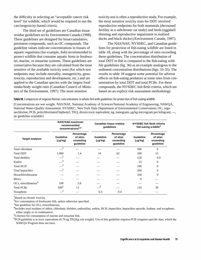
Significance to Ecosystems and Human Health 75
the difficulty in selecting an “acceptable cancer risk level” for wildlife, which would be required to use the carcinogenicity-based criteria.
The third set of guidelines are Canadian tissue residue guidelines set by Environment Canada (1998). These guidelines are designed for bioaccumulative, persistent compounds, such as OC compounds. The guideline values indicate concentrations in tissues of aquatic organisms (for example, fish) recommended to protect wildlife that consume aquatic biota in freshwa-ter, marine, or estuarine systems. These guidelines are conservative because they are calculated from the most sensitive of the available toxicity tests (for which test endpoints may include mortality, mutagenicity, geno-toxicity, reproduction and development, etc.) and are applied to the Canadian species with the largest food intake/body weight ratio (Canadian Council of Minis-ters of the Environment, 1997). The most sensitive
toxicity test is often a reproductive study. For example, the most sensitive toxicity tests for DDT involved reproductive endpoints for both mammals (decreased fertility in a subchronic rat study) and birds (eggshell thinning and reproductive impairment in mallard ducks and black ducks) (Environment Canada, 1997).
The NAS/NAE, NYSDEC, and Canadian guide-lines for protection of fish-eating wildlife are listed in table 18, along with the percentage of sites exceeding these guidelines. The concentration distribution of total DDT in fish is compared to the fish-eating wild-life guidelines (fig. 36) as an example analogous to the sediment concentration distributions (figs. 33-35). The results in table 18 suggest some potential for adverse effects on fish-eating predators at some sites from con-tamination by total DDT and total PCBs. For these compounds, the NYSDEC fish flesh criteria, which are based on an explicit risk assessment methodology
Table18. Comparison of organochlorine concentrations in whole fish with guidelines for protection of fish-eating wildlife
[Concentrations are wet weight. NAS/NAE, National Academy of Sciences/National Academy of Engineering; NAWQA, National Water-Quality Assessment; NYSDEC, New York State Department of Environmental Conservation; OC, orga-nochlorine; PCB, polychlorinated biphenyl; TEQ, dioxin toxic equivalent; ng, nanogram; µg/kg microgram per kilogram; —, no guideline available]
1Based on chronic toxicity.2For consumption of freshwater fish, unless otherwise specified.3See guideline for OCs, miscellaneous.4Includes total residues of aldrin, chlordane, dieldrin, endosulfan, endrin, HCH, heptachlor, heptachlor epoxide, lindane, and toxaphene,
either singly or in combination.5Criterion for consumption of marine and estuarine fish.6PCB guideline is in toxic equivalents (0.79 ng TEQ/kg wet weight). Use of this guideline requires PCB congener-specific data, which the
NAWQA Program does not have.
NAS/NAE maximum
recommended
concentrations1,2
Canadian tissue residue
guidelines
NYSDEC fish flesh criteria
fish-eating wildlife1
Target analytesGuideline
(µg/kg)
Percentage
of sites
exceeding
guideline
Guideline
(µg/kg)
Percentage
of sites
exceeding
guideline
Guideline
(µg/kg)
Percentage
of sites
exceeding
guideline
Total chlordane —3 — — — 500 0
Total DDT 1,000 1.4 14 62 200 12
Total dieldrin —3 — — — 120 0.9
Endrin —3 — — — 25 0
Total HCH —3 — — — 100 0
Total heptachlor —3 — — — 200 0
Hexachlorobenzene — — — — 330 0
Mirex — — — — 0 —
OCs, miscellaneous4 100 5.8 — — — —
Total PCBs 5005 13 —6 — 110 30
Toxaphene —3 — 6.3 0.4 — —

76 OCs and PCBs in Stream Sediment and Aquatic Biota—Initial Results, NAWQA, 1992–1995
10
0
20
30
40
50
60
70
80
90
100
0 1 2 3 4
NA
S/N
AE
maxim
um recom
mended tisssue concentration
NY
SD
EC
fish-flesh criterion
EP
A screening value (at 10E
-5 cancer risk)
FD
A action level
Canadian tissue residue guideline
W W WHH HH
Log (total DDT concentration, in micrograms per kilogram, in wet weight)
Per
cent
age
of s
ites
with
con
cent
ratio
ngr
eate
r th
an o
r eq
ual t
o in
dica
ted
valu
e
and on a more extensive toxicological database than the older NAS/NAE guidelines, were exceeded by measured concentrations in whole fish at 12 percent (total DDT) and 30 percent (total PCBs) of sites. For total DDT, the Canadian tissue residue guideline (which is much lower than the other two guidelines for this compound) was exceeded by measured concentra-tions in whole fish at 62 percent of sites. This Cana-dian guideline considers not only chronic toxicity, but potential carcinogenicity and reproductive effects (Canadian Council of Ministers of the Environment, 1997).
Human Health
Human health standards and guidelines are numerical values that indicate a threshold for potential effects on human health. Various human health stan-dards and guidelines exist for pesticides in fish and shellfish tissue. Strictly speaking, the tissue data col-lected by NAWQA are not appropriate for determina-tion of potential human health effects using these standards and guidelines for two reasons. First, the standards and guidelines are intended for comparison
with contaminant residues in edible fish tissue or shell-fish, whereas NAWQA fish data are for whole fish. Secondly, the fish and bivalves taxa sampled in NAWQA are not commonly consumed by people. The fish taxa sampled in NAWQA were mostly bottom feeders or omnivores, such as white sucker and com-mon carp. The bivalves sampled in NAWQA were the Asiatic clam (table 2). This is an (intentional) conse-quence of the NAWQA study design, which called for maximizing the probability of detecting organochlo-rine contaminants in the hydrologic system. This study objective was a major factor driving the selection of target taxa and the decision to analyze whole-body tis-sue (Crawford and Luoma, 1993).
Nonetheless, it is possible to compare NAWQA whole fish data with standards and guidelines for edi-ble fish tissue as a screening tool for identifying sites with some potential for human health effects. This screening process can be used to identify sites at which additional sampling and analysis of fish fillets may be warranted. Residues of HOCs, including OC pesticides and PCBs, generally are expected to be higher in whole fish than in edible fish tissue because muscle or fillets generally have lower fat contents than
Figure 36. Concentration distribution of total DDT in whole fish, shown in comparison with edible-fish consumption standards and guidelines for human health and whole-fish consumption guidelines for wildlife. Standards and guidelines are shown as vertical lines, designated as either human health (HH) or wildlife (W). FDA, Food and Drug Administration; NAS/NAE, National Academy of Sciences and National Academy of Engineering; NYSDEC, New York State Department of Environmental Conservation; EPA, U.S. Environmental Protection Agency.

Significance to Ecosystems and Human Health 77
does the whole fish (Niimi and Oliver, 1989). This means that if standards and guidelines for a given con-taminant in edible fish tissue are not exceeded by mea-sured concentrations of that contaminant in whole fish, then it is reasonable to conclude that these standards and guidelines are not likely to be exceeded by the res-idue in edible fish tissue either. However, if a particu-lar standard or guideline for edible fish tissue is exceeded by measured concentrations in whole fish, this indicates only that additional sampling and analy-sis of fish fillets may be warranted at that site.
In the screening analysis below, measured OC concentrations in whole fish at NAWQA sites were compared with one standard (U.S. Food and Drug Administration [FDA] action levels) and one guideline (EPA screening values) for the protection of human health. The FDA action level is an enforceable regula-tory limit for unavoidable pesticide residues in or on a food or animal feed (U.S. Food and Drug Administra-tion, 1990). Its purpose is to protect the general public from contaminants in fish shipped under interstate commerce (Reinert and others, 1991). FDA action lev-els exist for pesticides no longer registered for use in the United States, but that may be present as unavoid-able residues in fish or shellfish (such as organochlo-rine pesticides). Similarly, an FDA tolerance level exists for PCBs in fish and shellfish (U.S. Food and Drug Administration, 1984). FDA action levels are derived from FDA’s monitoring data, which provide an indication of the extent to which residues cannot be avoided by good agricultural or manufacturing prac-tices (U.S. Food and Drug Administration, 1990). Their development entails consideration of health effects to the general population plus other factors, such as analytical detections limits (U.S. Food and Drug Administration, 1990) and economic costs to the fishing industry (Reinert and other 1991). EPA screen-ing values were published as part of EPA’s guidance to state, local, regional, and tribal environmental health officials who are responsible for issuing fish advisories for non-commercial fish (U.S. Environmental Protec-tion Agency, 1994, 1995). EPA defined screening val-ues as concentrations of analytes in fish and shellfish that are of potential health concern and that can be used as guidelines against which levels of contamina-tion in similar tissue collected from the ambient envi-ronment can be compared (U.S. Environmental Protection Agency, 1995). Screening values were derived using an explicitly stated risk assessment methodology, assuming average values for consumer
body weight, meal size, and meal frequency. The screening analysis below assumes a body weight of 70 kg, a mean daily consumption rate of 6.5 g/d of fresh-water and estuarine fish over a 70-year lifetime, and that 80 percent of daily exposure comes from con-sumption of fish and shellfish. For potential carcino-gens, the screening value constitutes the concentration associated with a specified cancer risk level (the maxi-mum acceptable cancer risk level), which is generally between 10-7 and 10-4. The analysis below assumes a maximum acceptable cancer risk level of 10-5, a risk level that corresponds to one excess case of cancer per 100,000 individuals exposed over a 70-year lifetime. These assumptions are the same as those used by the U.S. Environmental Protection Agency (1995) to rep-resent the general adult population in the United States.
Table 19 lists the FDA action levels and EPA screening values for the OC analytes in the present study, along with EPA's carcinogenicity classification of each analyte (U.S. Environmental Protection Agency, 1995) into one of five cancer groups. These cancer groups are defined (U.S. Environmental Protec-tion Agency, 1986) as follows. Group A (human car-cinogen) consists of compounds for which there is sufficient evidence in epidemiological studies in humans to support casual association between expo-sure and cancer. Group B (probable human carcino-gen) consists of compounds for which there is limited evidence in epidemiological studies (Group B1) or sufficient evidence from animal studies (Group B2) to support causal association between exposure and can-cer. Group C (possible human carcinogen) consists of compounds for which there is limited or equivocal evi-dence from animal studies and inadequate or no data in humans to support causal association between expo-sure and cancer. Group D (not classified) consists of compounds for which there is inadequate or no human or animal evidence of carcinogenicity. Finally, group E (no evidence of carcinogenicity for humans) consists of compounds for which there is no evidence of carci-nogenicity in at least two adequate animal tests in dif-ferent species or in adequate epidemiological and animal studies. As mentioned previously, for analytes that are human carcinogens or probable human carcin-ogens (Cancer Group A or B), the EPA screening val-ues in table 19 correspond to a maximum acceptable cancer risk level of 10-5 (that is, 1 in 100,000).
In 1996, the U.S. Environmental Protection Agency (1996a) proposed new guidelines for carcino-

78 OCs and PCBs in Stream Sediment and Aquatic Biota—Initial Results, NAWQA, 1992–1995
gen risk assessment, which make substantial changes in the characterization of hazard and in the approach to dose-response assessment. These changes include replacing the cancer groups A through E with standard descriptors within a narrative presentation (“known/likely,” “not likely,” and “cannot be determined”), and considering the mode of action in characterizing haz-ard and in dose-response assessment. In cases where there is evidence of nonlinear dose-response, the pro-posed guidelines call for using a margin of exposure approach, rather than estimating the probability of response at low doses. However, the 1996 proposed guidelines have not been finalized by EPA, and cancer groups A through E are still used by EPA to character-ize contaminants in water (U.S. Environmental Protec-tion Agency, 1999). Therefore, the original EPA guidelines for carcinogen risk assessment (U.S. Envi-ronmental Protection Agency, 1986) are used in the following analysis of potential human health effects of
OC contaminants in fish as measured by NAWQA.The percentage of sites with measured concen-
trations that exceed FDA action levels and EPA screening values are listed in table 19. To illustrate the comparison of OC concentrations in whole fish with human health standards and guidelines, figure 36 shows the concentration distribution of DDT in whole fish. The FDA action level and the EPA screening value for total DDT are shown in figure 36 as vertical lines that intersect the cumulative frequency curve. Very few sites had residues in whole fish that exceeded any FDA action levels for OC compounds (table 19). The exceptions were total PCBs (for which the action level was exceeded at about 3 percent of sites) and total chlordane (at less than 1 percent of sites). Some-what higher frequencies of exceedance were observed for EPA screening values because these guidelines are much lower than the corresponding FDA action levels for all of the OC analytes except mirex and endrin.
Table19. Comparison of organochlorine concentrations in whole fish with edible-fish guidelines for protection of human health
[Because chemical concentrations are in whole fish, whereas standards and guidelines apply to edible fish tissue, exceedance indicates that additional sampling of game fish fillets may be warranted (see text for details). All concentrations are wet weight. EPA cancer group: B2, probable human carcinogen; C, possible human carcinogen; D, not classified; E, no evidence of carcinogenicity (see text for additional detail). FDA, Food and Drug Administration; EPA, U.S. Environmental Protection Agency; µg/kg, microgram per kilogram; —, no standard or guideline available]
1From U.S. Environmental Protection Agency (1995). 2From Food and Drug Administration (1990), unless otherwise specified. 3Based on chronic toxicity, unless otherwise specified. 4Not classified by EPA; however, classified as a probable human carcinogen by International Agency for Research on Cancer. 5Based on 1 in 100,000 cancer risk. 6FDA tolerance level (from Food and Drug Administration, 1984).
Target analytesEPA cancer
group1
FDA action level2EPA guidance for use in fish
advisories: Recommended
screening value1,3
Standard
(µg/kg)
Percent of sites
exceeding
standard
Guideline
(µg/kg)
Percent of sites
exceeding
guideline
Total chlordane B2 300 0.4 580 5.7
Total DDT B2 5,000 0 5 300 7.8
Total dieldrin B2 300 0 57 23
Endrin D/E 300 0 3,000 0
Total heptachlor B2 300 0 510 3
Hexachlorobenzene B2 300 0 510 0
Lindane B2/C — — 5 70 0
Mirex —4 100 0 2,000 0
Total PCBs B2 62,000 2.6 510 45
Toxaphene B2 5,000 0 5100 0.4

Significance to Ecosystems and Human Health 79
EPA screening values for edible fish tissue were exceeded by whole fish concentrations for a substan-tial percentage of sites for total PCBs (at 45 percent of sites) and total dieldrin (at 23 percent of sites). EPA screening values were exceeded less often for total DDT (at 8 percent of sites), total chlordane (at 6 per-cent of sites), total heptachlor (at 3 percent of sites), and toxaphene (at 0.4 percent of sites). Overall, 54 percent of NAWQA sites had whole fish residues that exceeded one or more EPA screening values for edible fish tissue. Even excluding total PCBs, for which the EPA screening value is particularly low, 26 percent of NAWQA sites had whole fish residues that exceeded one or more screening values for OC pesticides in edible-fish tissue. These results suggest that it may be worthwhile to monitor OC contaminant residues in edible tissue of game fish at the sites where one or more standards or guidelines were exceeded. These NAWQA data do not provide any information on whether residues in edible portions of game fish col-lected at these sites will exceed the applicable human health standards and guidelines, or are safe to eat.
All of the OC compounds for which EPA screening values are exceeded (see table 19) are classi-fied by EPA as potential human carcinogens (Group B2). Thus, the screening values in table 19 are associ-ated with a specified cancer risk (1 in 100,000). The choice of maximum acceptable cancer risk (in this case, 10-5, that is, 1 in 100,000) will strongly influence the frequency with which the guidelines are exceeded. For example, if the maximum acceptable cancer risk were tenfold higher (1 in 10,000), the screening value also would be tenfold higher and the frequency of exceedance would be much lower. In contrast, a ten-fold lower maximum acceptable cancer risk (1 in 1,000,000) would result in a tenfold lower screening value, and the frequency of exceedance would be much higher. The choice of an acceptable risk level is a risk management decision (U.S. Environmental Pro-tection Agency, 1995). EPA's policy is to accept cancer risk policies from the states in the range of 10-6 to 10-4 (U.S. Environmental Protection Agency, 1993a).
FDA action levels are considerably higher than EPA screening values for all of the compounds in table 19, except endrin and mirex, for which the reverse is true. Generally, several differences between FDA action levels and EPA screening values contribute to this discrepancy. First, FDA action levels apply to fish or fish products in interstate commerce, whereas EPA screening values, which are intended as guidance for
issuing fish consumption advisories, apply to noncom-mercial fish. Second, FDA action levels are based on a different risk assessment methodology than that used by EPA (Reinert and others, 1991). For example, EPA uses a more conservative approach to extrapolating from toxicity test results with rodents to estimates of toxicity in humans. Whereas EPA relies on a ratio of animal-to-human body surface areas, FDA uses a ratio of animal-to-human body weights. Both models are conservative, but the EPA model is more so. The EPA model results in a sixfold greater risk than the FDA model when data from rats are used and in a fourteen-fold greater risk when data from mice are used (Rein-ert and others, 1991). Third, FDA action levels are not based on health considerations alone, but also consider factors such as economic costs (Reinert and others, 1991) and analytical detection limits (U.S. Food and Drug Administration, 1990). Action levels are derived primarily from FDA's monitoring data, which provides an indication of the extent to which residues of a par-ticular pesticide cannot be avoided by good agricul-tural practice or by current good manufacturing practice (U.S. Environmental Protection Agency, 1993b). Thus, there is not the same direct link between levels of risk and levels of fish consumption that the EPA risk-based approach provides (Reinert and others, 1991). The EPA screening values for potential carcino-gens may be particularly conservative because they are based on a cancer potency factor that was estimated using a linearized multistage model of carcinogenicity. This model is conservative and assumes that there is a no-observed-adverse-effect-level for carcinogens; that is, exposure to even a very small amount of a sub-stance theoretically produces a finite increased risk of cancer (U.S. Environmental Protection Agency, 1989). Moreover, the cancer potency factor used is defined as the 95 percent upper bound estimate of the slope of the dose-response (cancer) curve. This may partially explain why the EPA screening values for endrin and mirex are actually higher than the FDA action levels. Endrin and mirex are the only compounds in table 19 that have not been classified as B2 carcinogens by EPA. Therefore, the EPA screening values for endrin and mirex were based on chronic toxicity, rather than carcinogenicity. Also, as noted previously, FDA action levels are not based exclusively on health effects (U.S. Food and Drug Administration, 1990), but also con-sider FDA monitoring data (U.S. Environmental Pro-tection Agency, 1993b). Historically and nationally, neither mirex nor endrin has been commonly detected

80 OCs and PCBs in Stream Sediment and Aquatic Biota—Initial Results, NAWQA, 1992–1995
in fish and shellfish relative to several of the other organochlorine compounds listed in table 19 (Nowell and others, 1999).
The EPA screening value for total PCBs in edi-ble fish at a 10-5 cancer risk level (10 µg/kg wet weight) is substantially lower than the analytical reporting limit for the NAWQA Program (50 µg/kg wet weight), so any detection of total PCBs in whole fish samples exceeds this guideline value. Besides the uncertainty inherent in procedures for calculating the screening value for a potential carcinogen, the PCB guideline has additional uncertainty because the chem-ical composition of total PCBs varies, and the toxicity and carcinogenicity of different PCB congeners also vary. EPA based its screening value for total PCBs on the cancer potency factor for Aroclor 1260, and rec-ommends determining total PCBs as Aroclor equiva-lents, then assuming that the mixture has comparable carcinogenicity to Aroclor 1260. The choice of Aro-clor 1260 was conservative in that it is a more potent carcinogen than Aroclors 1254 or 1242. However, it may not represent an upper bound risk because the PCB congener distribution in fish and shellfish tissue is usually different from, and may be more potent than, the parent Aroclor mixtures (U.S. Environmental Protection Agency, 1995). The U.S. Environmental Protection Agency (1995, p. 5–18) recognized the implications of such a low guideline value for PCBs: “[EPA] also recognizes that the current recommended [screening value] of 10 ppb for total PCBs will result in widespread exceedance in water bodies throughout the country and will drive virtually all fish and shell-fish monitoring programs into the risk assessment phase for PCBs. The decision on whether to issue a consumption advisory for PCBs at this level is one that must be made by risk managers in each State.”
Other Toxicity Concerns
The standards and guidelines used in the above analysis were developed considering both acute and chronic toxicity to aquatic organisms and wildlife, depending on the available data. However, except as noted previously, such guidelines generally do not consider certain more complex issues related to toxic-ity, such as the effect of chemical mixtures on toxicity and the potential for endocrine-disrupting effects on the development, reproduction, and behavior of fish and wildlife populations.
Effects of Chemical Mixtures
Organisms are likely to be exposed to mixtures of contaminants. For example, factor analysis of national sediment contaminant data from the NS&T program showed that most sediment contaminants occur together (National Oceanic and Atmospheric Administration, 1991). Thus, there is potential for tox-icological interactions among chemical contaminants. Possible interactions generally are categorized as antagonistic, when a mixture is less toxic than the chemicals considered individually; synergistic, when a mixture is more toxic than the chemicals considered individually; or additive, when a mixture has toxicity equivalent to the sum of the toxicities of the individual chemicals in the mixture. Chemicals in a particular class may have similar mechanisms of toxicity and produce similar effects. For example, most OC com-pounds induce the mixed-function oxidase system, which is present in fish, as well as in mammals. Prior or simultaneous exposure to chemicals that induce the same enzyme system may affect toxicity. In some cases, toxicity may be increased, whereas in others it may be decreased because of detoxification. Exposure to multiple OC contaminants has been shown to affect contaminant uptake and accumulation, as well as tox-icity. For example, mixtures of DDT and mirex showed more than additive effects on fish survival and reproduction (Koenig, 1977).
The guidelines used in assessing biological sig-nificance are intentionally conservative, and thus are intended to overestimate risk or toxicity associated with a given contaminant concentration. Most of these standards and guidelines, however, were based on sin-gle-species, single-chemical toxicity (or carcinogenic-ity) studies. If contaminants that co-occur in the environment have additive or synergistic effects, then standards and guidelines based on single-chemical toxicity tests may not be predictive of toxicity in the environment.
Developmental and Reproductive Effects
Many studies have raised concerns about poten-tial endocrine-disrupting effects of organic chemicals on wildlife and other animals, including humans (Col-born and Clement, 1992; Colborn and others, 1992; U.S. Environmental Protection Agency, 1997b). Sev-eral synthetic organic contaminants have been shown to have estrogenic activity in animals, including some persistent OC compounds that are detected in bed

Summary 81
sediment and aquatic biota, such as DDT, DDE, dico-fol, dieldrin, heptachlor, hexachlorobenzene, kepone, lindane and other HCH isomers, methoxychlor, mirex, some PCB congeners, and toxaphene (Colborn and others, 1992).
The endocrine system is important in regulating development and reproduction in animals, thus sug-gesting that chemical disruption of the endocrine sys-tem may cause abnormal sexual development and impaired reproduction. The evidence for causal rela-tions between synthetic chemical exposure and adverse effects from endocrine disruption is much stronger for fish, birds, and wildlife than it is for humans. The literature on this topic is rapidly growing because of its scientific importance and political con-troversy. A review of this literature is beyond the scope of this report. Additional information can be found in review books and articles (Colborn and Clement, 1992; Colborn and others, 1992; Hileman, 1994; Raloff, 1994a,b, 1995; U.S. Environmental Protection Agency, 1997b) and in the primary publications cited therein.
The EPA’s assessment and analysis of the effects of environmental endocrine disruption concluded that there is compelling evidence that the endocrine sys-tems of certain fish and wildlife have been disturbed by chemical contaminants in their habitats (U.S. Envi-ronmental Protection Agency, 1997b). The chemicals identified include several OC compounds commonly detected in bed sediment and aquatic biota of hydro-logic systems (for example, DDT and PCBs). More-over, chemicals that affect fish and wildlife in their natural habitats also have been shown to cause similar effects in laboratory animal tests. However, it is not clear (U.S. Environmental Protection Agency, 1997b) whether the adverse effects observed at various sites are widespread or confined to specific areas and, in many cases, alternative explanations cannot be ruled out.
The evidence in humans is less definitive than for wildlife. Exposure to endocrine-disrupting syn-thetic chemicals has been suggested as contributing to the increased incidence of several pathologies in humans during the last 50 years, such as increased rates of breast and prostate cancers in the United States, an increase in ectopic pregnancies in the United States, an increase in cryptorchidism in the United Kingdom, and a decrease in sperm count worldwide (Colborn and Clement, 1992). However, with few
exceptions (for example, diethylstilbestrol, dioxin, and DDT/DDE), a causal relation between human expo-sure to an environmental contaminant and endocrine disruption resulting in an adverse effect on human health has not been established (U.S. Environmental Protection Agency, 1997b). The EPA concluded that exposure to a single estrogenic synthetic chemical at current environmental concentrations is probably insufficient to cause adverse effects in human adults. More information is needed to determine whether this is true for the human fetus or newborn. Other data gaps include the effects of chemicals operating an non-estrogenic receptor sites to stimulate or inhibit estro-genic or other responses, and the effect of chemical mixtures on endocrine disruption (U.S. Environmental Protection Agency, 1997b).
Certain guidelines for protection of aquatic life and wildlife for organochlorine insecticides did con-sider certain reproductive effects (for example, egg-shell thinning in birds). However, less obvious effects on reproduction may occur on exposure to very low levels and may not be observed until long after the period of exposure. In some cases, effects may not be observed until subsequent generations mature (Col-born and Clement, 1992). Except possibly for Cana-dian tissue residue guidelines, such effects generally are not taken into account when using existing guide-lines to assess biological significance. Because of these limitations, it is possible that adverse effects on aquatic organisms or wildlife may occur at lower con-centrations than indicated by the standards and guide-lines.
SUMMARY
This report summarizes the occurrence and dis-tribution of 33 organochlorine compounds in stream bed sediment, fish, and bivalves sampled by the National Water-Quality Assessment (NAWQA) Pro-gram between 1991 and 1994. The compounds included historically used organochlorine insecticides (DDT and metabolites, chlordane and its various com-ponents, and dieldrin), some currently used pesticides (permethrin and dacthal) and some industrial chemi-cals and byproducts (PCBs and HCB). The samples were collected at approximately 500 sites in 19 large hydrologic basins throughout the United States and provide a national view of levels of hydrophobic con-taminant levels in these rivers.

82 OCs and PCBs in Stream Sediment and Aquatic Biota—Initial Results, NAWQA, 1992–1995
Detection frequencies among media were gener-ally highest in fish, less frequent in sediment, and (for most analytes) very low in bivalves. The most com-monly detected compounds were DDT and its metabo-lites DDD and DDE, total PCBs, dieldrin, and the members of the chlordane group (cis- and trans-chlor-dane, and cis- and trans-nonachlor). The compound detected most frequently at sampling sites in all three types of sampling media was p,p′-DDE: 80 percent in fish, 39 percent in sediment, and 29 percent in bivalves. All of the p,p′ isomers of DDT and its metab-olites were detected more frequently than the o,p′ iso-mers, which reflects the higher ratio of p,p′-DDT to o,p′-DDT released to the environment in technical grade DDT. These data were not censored to a com-mon reporting level among the target analytes. There-fore, detection frequencies reflected differences in individual reporting limits, as well as environmental occurrence. Certain analytes (pentachloroanisole, total PCBs, and toxaphene in sediment; total PCBs and tox-aphene in fish) had much higher reporting limits than most of the others, so their detection frequencies were not directly comparable to the other analytes with the lower reporting limits.
Sediment and biota (fish and bivalves) were sampled in NAWQA because both of these media accumulate hydrophobic compounds and, thus, can provide both a means of determining long-term water-quality trends and identifying sources of contamina-tion in rivers and streams. Together, sediment and biota comprise dual lines of evidence for contamina-tion of a hydrologic system. A positive, albeit weak, correlation between concentrations of compounds in sediment and fish was observed for sites at which both media were sampled on the same day in this study. These correlations were generally stronger when the concentrations in sediment and biota were normalized to organic carbon and lipid content, respectively; yet there was still considerable variability in the relation. A positive correlation was also observed between fish and bivalve concentrations at paired sites. Lipid nor-malization appeared to strengthen this relation consid-erably; however, the dearth of available paired sites (only seven) for bivalves made this observation some-what tenuous.
The sampling sites were classified as integrator, background, pasture/rangeland, cropland, or urban on the basis of their dominant land use. (Background regions were defined as areas in which the total area of all land uses where chemical use is expected to be low
[forested land, rangeland, tundra, bare ground, and exposed rock] was greater than 95 percent of the site's total basin area.) The frequency of detection for most of the OC compounds in all three media were gener-ally highest in the urban basins and lowest in the back-ground basins. This observation was consistent with the expected use of organochlorine chemicals within these two categories. Some differences in detection patterns were observed among the land-use groups for specific compounds compared to the national sum-mary. Several pesticides, both historically used (tox-aphene and aldrin) and currently used (cis- and trans-permethrin), were detected only at the cropland sites, which is consistent with the agricultural use of these compounds. Total PCBs, which had a fairly low detec-tion occurrence nationally, were found in every urban fish sample. Because PCBs have primarily an indus-trial source, it is to be expected that they would be found most frequently in urban areas. Within a given land-use classification, detection frequencies were not related to basin size.
Temporal trends were evaluated by comparing the concentrations of organochlorine compounds in fish between NAWQA and the National Contaminant Biomonitoring Program (NCBP, 1969–1986). No equivalent program for fluvial bed sediments was available to allow temporal comparisons. The NCBP (1969–1986) / NAWQA (1991–1995) comparison suggests that residues of the most commonly detected pesticides in whole fish have declined nationally. The largest declines occurred during the 1970s, although NAWQA data suggests substantial declines for total chlordane, dieldrin, and total DDT during the 1990s. Total PCB concentrations at most NAWQA sites were lower than at most NCBP sites, but some NAWQA sites had extremely high concentrations, even com-pared with NCBP data for the 1970s. Differences in site selection strategies between the NAWQA and NCBP studies may have affected this comparison.
Numerous standards and guidelines have been developed that indicate pesticide levels expected to cause adverse effects on aquatic organisms, wildlife, or human health. Bed sediment concentrations of most organochlorine compounds did not exceed sediment-quality guidelines, suggesting no adverse effects on aquatic life. The exceptions were the four most com-monly detected compounds or compound groups: total DDT (exceedances at 37 percent of sites), total chlor-dane (19 percent), dieldrin (14 percent), and total PCBs (6 percent). The New York Department of
References Cited 83
Environmental Conservation has established fish-flesh criteria for the protection of fish-eating wildlife. These wildlife criteria, which are based on an explicit risk assessment methodology, were exceeded by measured concentrations in whole fish at 12 and 30 percent of sites for total DDT and total PCBs, respectively. Strictly speaking, the tissue data collected by NAWQA are not appropriate for comparison with human-health standards and guidelines, which apply to edible fish tissue. Nonetheless, it is possible to use comparison of NAWQA whole fish data with standards and guide-lines for edible fish tissue as a screening tool for potential human health effects; in this case, exceed-ance would indicate where it may be worthwhile to monitor organochlorine compounds in game fish fil-lets. Very few sites had residues in whole fish that exceeded FDA action levels. The exceptions were total PCBs at about 3 percent of sites and total chlordane at 0.4 percent of sites. Somewhat higher frequencies of exceedance were observed for EPA screening values, which are guidelines provided by EPA as part of that agency’s guidance to state, local, and tribal health offi-cials responsible for issuing fish-consumption adviso-ries. Overall, 54 percent of NAWQA sites had whole fish residues exceeding one or more EPA screening values for edible fish tissue. The compounds responsi-ble for these exceedances were total PCBs (with exceedances at 45 percent of sites), dieldrin (23 per-cent of sites), total DDT (8 percent of sites), total chlo-rdane (6 percent of sites), total heptachlor (3 percent of sites), and toxaphene (less than 1 percent of sites). These results suggest that it may be worthwhile to monitor organochlorine residues in edible tissue of game fish at the sites where one or more standards or guidelines were exceeded.
REFERENCES CITED
Agee, B.A., 1986, DDT in the Salinas Valley: A special report on the probable source of technical grade DDT found in the Blanco Drain near Salinas, California: Cal-ifornia State Water Resources Control Board, Division of Water Quality, Water Quality Monitoring Report 86-2, 49 p.
Aguilar, A., 1984, Relationship of DDE/DDT in marine mammals to the chronology of DDT input into the eco-system: Canadian Journal of Fisheries and Aquatic Sci-ence, v. 41, p. 840–844.
Anderson, J.R., Hardy, E., Roach, J., and Witmer, R., 1975, A land use and land cover classification system for use
with remote sensor data: U.S. Geological Survey Pro-fessional Paper 964, 28 p.
Andrilenas, P.A., 1974, Farmers’ use of pesticides in 1971—Quantities: U.S. Department of Agriculture, Economic Research Service, Agricultural Economic Report series, no. 252, 56 p.
Arruda, J.A., Cringan, M.S., Gilliland, D., Haslouer, S.G., Fry, J.E., Broxterman, R., and Brunson, K.L., 1987, Correspondence between urban areas and the concen-trations of chlordane in fish from the Kansas River: Bul-letin of Environmental Contamination and Toxicology, v. 39, p. 563–570.
Barnett, J.R., and Dorough, H.W., 1974, Metabolism of chlo-rdane in rats: Journal of Agriculture and Food Chemis-try, v. 22, p. 612–619.
Barrick, R., Becker, S., Brown, L., Beller, H., and Pastorok, R., 1988, Sediment quality values refinement: 1988 update and evaluation of Puget Sound AET, Volume. 1: Prepared for the Puget Sound Estuary Program. Office of Puget Sound, by PTI Environmental Services, Belle-vue Washington, 144 p.
Bedard, D.L., and Quensen, J.F., III, 1995, Microbial reduc-tive dechlorination of polychlorinated biphenyls, in Young, L.Y., and Cerniglia, C.E., eds., Microbial trans-formation and degradation of toxic organic chemicals: New York, Wiley-Liss, p. 127–216.
Bevenue, A., Hylin, J.W., Kawano, Yoshihiko, and Kelley, T.W., 1972, Organochlorine pesticide residues in water, sediment, algae, and fish, Hawaii—1970–1971: Pesti-cide Monitoring Journal, v. 6, no. 1, p. 56–64.
Brooks, G.T., 1974, Technology and application, v. 1 of Chlorinated insecticides: Cleveland, Ohio, CRC Press.
Bustos, S., Denegri, J.C., Diaz, F., and Tchernitchin, A.N., 1988, p,p´-DDT is an estrogenic compound: Bulletin of Environmental Contamination and Toxicology, v. 41, p. 496–501.
Butler, P.A., 1973, Organochlorine residues in estuarine mol-lusks, 1965–1972—National Pesticides Monitoring Program: Pesticide Monitoring Journal, v. 6, p. 238–362.
Butler, P.A., Kennedy, C.D., and Schutzmann, R.L., 1978, Pesticide residues in estuarine mollusks, 1977 versus 1972—National Pesticide Monitoring Program: Pesti-cide Monitoring Journal, v. 12, p. 99–101.
Butler, P.A., and Schutzmann, R.L., 1978, Residues of pesti-cides and PCBs in estuarine fish, 1972–1976—National Pesticide Monitoring Program: Pesticide Monitoring Journal, v. 12, p. 51–59.
Canadian Council of Ministers of the Environment, 1997, A protocol for the derivation of Canadian tissue residue guidelines for the protection of wildlife that consume aquatic biota.

84 OCs and PCBs in Stream Sediment and Aquatic Biota—Initial Results, NAWQA, 1992–1995
———1998, Canadian sediment quality guidelines for the protection of aquatic life: Introduction and summary tables, in Canadian environmental quality guidelines: Winnipeg, Canada, Canadian Council of Ministers of the Environment, Water Quality Guidelines Task Group, accessed December 6, 1998, at URL http://www.ec.gc.ca/ceqg-rcqe/sediment.htm/
Clark, D.R., Jr., and Krynitsky, A.J., 1983, DDT: Recent con-tamination in New Mexico and Arizona?: Environment, v. 25, no. 5, p. 27–31.
Colborn, Theo, and Clement, C.R,, eds., 1992, Chemically-induced alterations in sexual and functional develop-ment: The wildlife/human connection: Princeton, N.J., Princeton Scientific Publishing, Advances in Modern Environmental Toxicology series, v. 21, 403 p.
Colborn, Theo, vom Saal, F.S., and Soto, A.M., 1992, Devel-opmental effects of endocrine-disrupting chemicals in wildlife and humans: Environmental Health Perspec-tives, v. 101, no. 5, p. 378–384.
Crawford, J.K., and Luoma, S.N., 1993, Guidelines for stud-ies of contaminants in biological tissues for the National Water-Quality Assessment Program: U.S. Geological Survey Open-File Report 92-494, 69 p.
Dearth, M.A., and Hites, R.A., 1991, Complete analysis of technical chlordane using negative ionization mass spectrometry: Environmental Science and Technology, v. 25, p. 245–254.
Eichers, T., Andrilenas, P., and Anderson, T.W., 1978, Farm-ers’ use of pesticides in 1976: U.S. Department of Agri-culture, Economics, Statistics, and Cooperative Service, Agricultural Economic Report series, no. 418, 58 p.
Eichers, T., Andrilenas, P.A., Blake, H., Jenkins, R., and Fox, A., 1970, Quantities of pesticides used by farmers in 1966: U.S. Department of Agriculture, Economic Research Service, Agricultural Economic Report series, no. 179, 61 p.
Eichers, T., Andrilenas, P.A., Jenkins, R., and Fox, A., 1968, Quantities of pesticides used by farmers in 1964: U.S. Department of Agriculture, Economic Research Ser-vice, Agricultural Economic Report series, no. 131, 37 p.
Environment Canada, 1997, Canadian tissue residue guide-lines for DDT for the protection of wildlife consumers of aquatic biota: Quebec, Canada, Environment Can-ada, Guideline and Standards Division, Environment Canada, Quebec.
———1998, Canadian tissue residue guidelines for the pro-tection of wildlife consumers of aquatic biota: Sum-mary table, in Canadian tissue residue guidelines: Winnipeg, Canada, Canadian Council of Ministers of the Environment, Water Quality Guidelines Task Group, accessed December 6, 1998, at URL http://www.ec.gc.ca/ceqg-rcqe/sediment.htm/
Erickson, M.D., 1997, Analytical chemistry of PCBs (2nd ed.): Boca Raton, Fla., Lewis Publishers, 667 p.
Esworthy, R.F., 1987, Incremental benefit analysis: Restricted use of all pesticides registered for subterra-nean termite control: U.S. Environmental Protection Agency, Benefits and Use Division, Economic Analysis Branch.
Feltz, H.R., and Culbertson, J.K., 1972, Sampling proce-dures and problems in determining pesticide residues in the hydrologic environment: Pesticide Monitoring Jour-nal, v. 6, p. 171–178.
Feltz, H.R., Sayers, W.T., and Nicholson, H.P., 1971, National monitoring program for the assessment of pes-ticide residues in water: Pesticide Monitoring Journal, v. 5, p. 54–59.
Feroz, M., and Khan, M.A.Q., 1979, Metabolism, tissue dis-tribution, and elimination of cis-[14C]chlordane in the tropical freshwater fish Cichlasoma sp.: Journal of Agriculture and Food Chemistry, v. 27, p. 1190–1197.
Foreman, W.T., Conner, B.F., Furlong, E.T., Vaught, D.G., and Merten, L.M., 1995, Methods of analysis by the U. S. Geological Survey National Water Quality Labo-ratory: Determination of organochlorine pesticides and polychlorinated biphenyls in bottom sediment by dual capillary-column gas chromatography with electron-capture detection: U.S. Geological Survey Open-File Report 95-140, 78 p.
Foreman, W.T., and Gates, P.M., 1997, Matrix-enhanced degradation of p,p'-DDT during gas chromatographic analysis: A consideration: Environmental Science and Technology, v. 31, no. 3, p. 905–910.
Fries, G.F., 1972, Degradation of chlorinated hydrocarbons under anaerobic conditions, in Faust, S.D., ed., Fate of organic pesticides in the aquatic environment: Ameri-can Chemical Society Advances in Chemistry series, no. 111, p. 256–270.
Fry, D.M., and Toone, C.K., 1981, DDT-induced feminiza-tion of gull embryos: Science, v. 213, p. 922–924.
Fry, D.M., Toone, C.K., Speich, S.M., and Peard, R.J., 1987, Sex ratio skew and breeding patterns of gulls: Demo-graphic and toxicological considerations: Studies in Avian Biology, v. 10, p. 26–43.
Gianessi, L.P., and Puffer, C.A., 1992, Insecticides use in U.S. crop production: Washington, D.C., Resources for the Future, Quality of the Environment Division, vari-ously paged.
Gilliom, R.J., Alexander, R.B., and Smith, R.A., 1985, Pes-ticides in the Nation's rivers, 1975–1980, and implica-tions for future modeling: U.S. Geological Survey Water-Supply Paper 2271, 26 p.
Gilliom, R.J., Alley, W.M., and Gurtz, M.E., 1995, Design of the National Water-Quality Assessment Program: Occurrence and distribution of water-quality condi-tions: U. S. Geological Survey Circular 1112, 33 p.

References Cited 85
Gilliom, R.J., and Clifton, D.G., 1990, Organochlorine pes-ticide residues in bed sediments of the San Joaquin River, California: Water Resources Bulletin, v. 26, no. 1, p. 11–24.
Gilliom, R.J., and Thelin, G.P., 1997, Classification and mapping of agricultural land for national water-quality assessment: U.S. Geological Survey Circular 1131, 70 p.
Golden, K.A., 1994, Organochlorines in Lake Michigan sed-iments: Minneapolis, Minn., University of Minnesota, M.S. thesis, 205 p.
Hanson, P.J., Evans, D.W., Fortner, A.R., and Siewicki, T.C., 1989, Contaminant assessment for the southeast Atlan-tic and Gulf of Mexico coasts: 1984 (cycle 1) and 1985 (cycle 2). Results of the National Benthic Surveillance Project: U.S Department of Commerce, National Oce-anic and Atmospheric Administration, National Marine Fisheries Service, Southeast Fisheries Center, Beaufort Laboratory, 86 p., 1 appendix.
Helsel, D.R., and Hirsch, R.M., 1992, Statistical methods in water resources: Amsterdam, Holland, Elsevier, Studies in Environmental Science series, v. 49, 522 p.
Henderson, C., Johnson, W.L., and Inglis, A., 1969, Orga-nochlorine insecticide residues in fish (National Pesti-cide Monitoring Program): Pesticide Monitoring Journal, v. 3, p. 145–171.
Henderson, C., Inglis, A., and Johnson, W.L., 1971, Orga-nochlorine insecticides in fish—fall 1969: National Pesticide Monitoring Program: Pesticide Monitoring Journal, v. 5, p. 1–11.
Hermanson, M.H., Christensen, E.R., Buser, D.J., and Chen, L.M., 1991, Polychlorinated biphenyls in dated sedi-ment cores from Green Bay and Lake Michigan: Jour-nal of Great Lakes Research, v. 17, no. 1, p. 94–108.
Hileman, Bette, 1994, Environmental estrogens linked to reproductive abnormalities, cancer: Chemical and Engineering News, v. 72, no. 5, p. 19–23.
Hitt, K.J., 1994, Refining 1970's land-use data with 1990 population data to indicate new residential develop-ment: U.S. Geological Survey Water-Resources Investi-gation Report 94-4250, 15 p.
Howard, P.H., Boethling, R.S., Javis, W.F., Meylan, W.M., and Michalenko, E.M., 1991, Handbook of environ-mental degradation rates: Chelsea, Mich., Lewis Pub-lishers, 725 p.
Jeremiason, J.D., Hornbuckle, K.C., and Eisenreich, S.J., 1994, PCBs in Lake Superior, 1978–1992: Decreases in water concentrations reflect loss by volatilization: Envi-ronmental Science and Technology, v. 28, no. 5, p. 903–914.
Johnson, A., Norton, D., and Yake, B., 1988, Persistence of DDT in the Yakima River drainage, Washington: Archives of Environmental Contamination and Toxicol-ogy, v. 17, p. 289–297.
Johnson, L.L., Stehr, C.M., Olson, O.P., Myers, M.S., Pierce, S.M., McBain, B.B., and Varanasi, Usha, 1992, National Benthic Surveillance Project: Northeast coast: Fish histopathology and relationships between lesions and chemical contaminants (1987–89): U.S. Department of Commerce, National Oceanic and Atmospheric Administration, National Marine Fisher-ies Service, Northwest Fisheries Science Center, NOAA Technical Memorandum NMFS-NWFSC-4, 96 p.
Johnson, L.L., Stehr, C.M., Olson, O.P., Myers, M.S., Pierce, S.M., Wigren, C.A., McCain, B.B., and Varanasi, Usha, 1993, Chemical contaminants and hepatic lesions in winter flounder (Pleuronectes americanus) from the northeast coast of the United States: Environmental Science and Technology, v. 27, no. 13, p. 2759–2771.
Karickhoff, S.W., Brown, D.S., and Scott, T.A., 1979, Sorption of hydrophobic pollutants on natural sedi-ments: Water Research, v. 13, p. 241–248.
Kawano, M., Inoue, T., Wada, T., Hidaka, H., and Tatsukawa, R., 1988, Bioconcentration and residue patterns of chlo-rdane compounds in marine mammals: Invertebrates, fish, mammals, and seabirds: Environmental Science and Technology, v. 22, p. 792–797.
Khan, M.A.Q., Sudershan, P., Feroz, M., and Podowski, A.A., 1981, Biotransformations of cyclodienes and their photoisomers and hexachlorocyclopentadiene in mammals and fish, in Khan, M.A.Q., and Stanton, R.H., eds., Toxicology of halogenated hydrocarbons: Health and ecological effects: New York, Pergamon, p. 271–288.
Koenig, C.C., 1977, The effects of mirex alone and in com-bination on the reproduction of a salt marsh cyprin-odont fish, Adinia xenica, in Vernberg, F.J., Calabrese, A., and Thurberg, F.P., eds., Physiological responses of marine biota to pollutants: New York, Academic Press, p. 357–376.
Larson, S.J., Capel, P.D., and Majewski, M.S., 1997, Pesti-cides in suface waters: Distribution, trends, and govern-ing factors: Chelsea, Mich., Ann Arbor Press, Pesticides in the Hydrologic System series, v. 3, 373 p.
Leiker, T.J., Madsen, J.E., Deacon, J.R., and Foreman, W.T., 1995, Methods of analysis by the U.S. Geological Sur-vey National Water Quality Laboratory: Determination of chlorinated pesticides in aquatic tissue by capillary-column gas chromatography with electron-capture detection: U.S. Geological Survey Open-File Report 94-710, 42 p.
Lichtenstein, E., Fuhrenmann, T.W., and Schulz, K.R., 1971, Persistence and vertical distribution of DDT, lindane, and aldrin residues 10 and 15 years after a single soil application: Journal of Agriculture and Food Chemis-try, v. 19, p. 718–721.

86 OCs and PCBs in Stream Sediment and Aquatic Biota—Initial Results, NAWQA, 1992–1995
Long, E.R., MacDonald, D.D., Smith, S.L., and Calder, F.D., 1995, Incidence of adverse biological effects within ranges of chemical concentrations in marine and estua-rine sediments: Environmental Management, v. 19, no. 1, p. 81–97.
Long, E.R., and Morgan, L.G., 1991, The potential for bio-logical effects of sediment-sorbed contaminants tested in the National Status and Trends Program: U.S. Department of Commerce, National Oceanic and Atmospheric Administration, National Ocean Service, NOAA Technical Memorandum NOS OMA 52, vari-ously paged.
MacDonald, D.D., 1994, Development and evaluation of sediment quality assessment guidelines, v. 1 of Approach to the assessment of sediment quality in Flor-ida coastal water: MacDonald Environmental Services (Ladysmith, B.C.) report prepared for Florida Depart-ment of Environmental Protection, Office of Water Pol-icy, Tallahassee, Florida, 123 p.
Majewski, M.S., and Capel, P.D., 1995, Pesticides in the atmosphere: Distribution, trends, and governing fac-tors: Chelsea, Mich., Ann Arbor Press, Pesticides in the Hydrologic System series, v. 1, 214 p.
Manchester, J.B., 1993, The role of porewater in the remobi-lization of sediment-bound polychlorinated biphenyl congeners: Madison, Wis., University of Wisconsin, Ph.D. dissertation, 584 p.
Mayer, F.L., and Ellersieck, M.R., 1986, Manual of acute toxicity: Interpretation and data base for 410 chemicals and 66 species of freshwater animals. U. S. Fish and Wildlife Service, Resource Publication 160, variously paged.
Mischke, Tom, Brunetti, K., Acosta, V., Weaver, D., and Brown, M., 1985, Agricultural sources of DDT residues in California's environment: A Report Prepared in Response to House Resolution No. 53 (1984): Califor-nia Department of Food and Agriculture, Environmen-tal Hazards Assessment Program, 42 p.
Mullin, M.D., Pochini, C.M., McCrindle, S., Romkes, M., Safe, S.H., and Safe, L.M., 1984, High-resolution PCB analysis: Synthesis and chromatographic properties of all 209 PCB congeners: Environmental Science and Technology, v. 18, p. 468–476.
Myers, M.S., Stehr, C.M., Olson, O.P., Johnson, L.L., McCain, B.B., Chan, S., and Varanasi, Usha, 1993, National Benthic Surveillance Project: Pacific coast: fish histopathology and relationships between toxico-pathic lesions and exposure to chemical contaminants for cycles I to V (1984–88): U.S. Department of Com-merce, National Oceanic and Atmospheric Administra-tion, National Marine Fisheries Service, Northwest Fisheries Science Center, NOAA Technical Memoran-dum NMFS-NWFSC-6, 160 p.
National Academy of Sciences and National Academy of Engineering, 1973, Water quality criteria, 1972: U.S. Environmental Protection Agency, EPA R3-73-033, 594 p.
National Oceanic and Atmospheric Administration, 1988, A summary of selected data on chemical contaminants in sediments collected during 1984, 1985, 1986, and 1987: U.S. Department of Commerce, National Oce-anic and Atmospheric Administration, National Ocean Service, NOAA Technical Memorandum NOS OMA 44, variously paged.
———1989, A summary of data on tissue contaminantion [sic] from the first three years (1986–1988) of the Mus-sel Watch Project: U.S. Department of Commerce, National Oceanic and Atmospheric Administration, National Ocean Service, NOAA Technical Memoran-dum NOS OMA 49, variously paged.
———1991, Second summary of data on chemical contam-inants in sediments from the National Status and Trends Program: U.S. Department of Commerce, National Oceanic and Atmospheric Administration, National Ocean Service, NOAA Technical Memorandum NOS OMA 59, variously paged.
Newell, A.J., Johnson, D.W., and Allen, L.K., 1987, Niagara River biota contamination project: Fish flesh criteria for piscivorous wildlife: New York Department of Environ-mental Conservation, Division of Fish and Wildlife, Bureau of Environmental Protection, Technical Report 87-3, 182 p.
Niimi, A.J., and Oliver, B.G., 1989, Distribution of polychlo-rinated biphenyl congeners and other halocarbons in whole fish and muscle among Lake Ontario salmonids: Environmental Science and Technology, v. 23, p. 83–88.
Nowell, L.H., Capel, P.D., and Dileanis, P.D., 1999, Pesti-cides in stream sediment and aquatic biota: Distribu-tion, trends, and governing factors: Boca Raton, Fla., CRC Press, Pesticides in the Hydrologic System series, v. 4, 1040 p.
Nowell, L.H., and Resek, E.A., 1994, National standards and guidelines for pesticides in water, sediment, and aquatic organisms: Application to water-quality assessments: Reviews of Environmental Contamination and Toxicology, v. 140, p. 1–164.
O'Connor, T.P., 1992, Mussel Watch: Recent trends in coastal environmental quality: Results from the first five years of the NOAA Mussel Watch Program: U.S. Department of Commerce, National Oceanic and Atmospheric Administration, National Ocean Service, 46 p.
Persaud, D., Jaagumagi, R., and Hayton, A., 1993, Guide-lines for the protection and management of aquatic sed-iment quality in Ontario: [Toronto], Canada, Ontario

References Cited 87
Ministry of the Environment and Energy, Water Resources Branch, variously paged.
Raloff, J., 1994a, The gender benders: Are environmental hormones emaseulating wildlife?: Science News, v. 145, no. 2, p. 24–27.
———1994a, That feminine touch: Are men suffering from prenatal or childhood exposure to "hormonal" toxi-cants?: Science News, v. 145, no. 4, p. 56–58.
———1995, Beyond estrogens, why unmasking hormone-mimicking pollutants proves so challenging: Science News, v. 148, no. 3, p. 44–46.
Reinert, R.E., Knuth, B.A., Kamrin, M.A., and Stober, Q.J., 1991, Risk assessment, risk management, and fish con-sumption advisories in the United States: Fisheries, v. 16, no. 6, p. 5–12.
Rinella, J.F., Hamilton, P.A., and McKenzie, S.W., 1993, Persistence of the DDT pesticide in the Yakima River Basin, Washington: U.S. Geological Survey Circular 1090, 24 p.
Rinella, J.F., McKenzie, S.W., Crawford, J., Foreman, W.T., and Fuhrer, G.J., 1996, Surface water-quality assess-ment of the Yakima River Basin, Washington: Distribu-tion of pesticides and other organic compounds in water, sediment, and aquatic biota, 1987–1991: U.S. Geological Survey Water-Supply Paper 2354B, 180 p.
Rinella, J.F., McKenzie, S.W., Crawford, J.K., Foreman, W.T., Gates, P.M., Fuhrer, G.J., and Janet, M.L., 1992, Surface-water-quality assessment of the Yakima River Basin, Washington: Pesticide and other trace-organic-compound data for water, sediment, soil, and aquatic biota, 1987–91: U.S. Geological Survey Open-File Report 92-644, 154 p.
SAS Institute, 1989, SAS/STAT User's Guide (4th ed.): Cary, N.C., SAS Institute, version 6, v. 2.
Schmitt, C.J., Ludke, J.L., and Walsh, D.F., 1981, Orga-nochlorine residues in fish: National Pesticide Monitor-ing Program, 1970–74: Pesticide Monitoring Journal, v. 14, p. 136–206.
Schmitt, C.J., Ribick, M.A., Ludke, J.L., and May, T.W., 1983, National Pesticide Monitoring Program: Orga-nochlorine residues in freshwater fish, 1976–79: U.S. Fish and Wildlife Service, Resource Publication 152, 62 p.
Schmitt, C.J., Zajicek, J.L., and Peterman, P.H., 1990, National Contaminant Biomonitoring Program: Resi-dues of organochlorine chemicals in U.S. freshwater fish, 1976–1984: Archives of Environmental Contami-nation and Toxicology, v. 19, no. 5, p. 748–781.
Schmitt, C.J., Zajicek, J.L., and Ribick, M.A., 1985, National Pesticide Monitoring Program: Residues of organochlorine chemicals in freshwater fish, 1980–1981: Archives of Environmental Contamination and Toxicology, v. 14, p. 225–260.
Schwemmer, B., Cochrane, W.P., and Polen, P.B., 1970, Oxychlordane, animal metabolite of chlordane: Isola-tion and synthesis: Science, v. 169, p. 1087.
Shelton, L.R., and Capel, P.D., 1994, Guidelines for collect-ing and processing samples of stream bed sediment for analysis of trace elements and organic contaminants for the National Water-Quality Assessment Program: U.S. Geological Survey Open-File Report 94-458, 20 p.
Sovocool, G.W., Lewis, R.G., Harless, R.L., Wilson, N.K., and Zehr, R.D., 1977, Analysis of technical chlordane by gas chromatography/mass spectrometry: Analytical Chemistry, v. 49, p. 734–740.
Street, J.C., and Blau, S.E., 1972, Oxychlordane: Accumula-tion in rat adipose tissue on feeding chlordane isomers or technical chlordane: Journal of Agriculture and Food Chemistry, v. 20, p. 395–397.
Swackhamer, D.L., and Armstrong, D.E., 1988, Horizontal and vertical distribution of PCBs in southern Lake Michigan sediments and the effect of Waukegan Harbor as a point source: Journal of Great Lakes Research, v. 14, p. 277–290.
Tanita, R., Johnson, J.M., Chun, M., and Maciolek, J., 1976, Organochlorine pesticides in the Hawaii Kai marina, 1970–74: Pesticide Monitoring Journal, v. 10, p. 24–29.
Tashiro, S., and Matsumura, F., 1977, Metabolic routes of cis- and trans-chlordane in rats: Journal of Agriculture and Food Chemistry, v. 25, p. 872-880.
U.S. Bureau of the Census, 1991, Census of population and housing, 1990: Public Law 94-171 data, machine-read-able data files.
U.S. Environmental Protection Agency, 1975, DDT, a review of scientific and economic aspects of the decision to ban its use as a pesticide: U.S. Environmental Protection Agency, EPA-540/1-75-022, 300 p.
———1980, Ambient water quality criteria for aldrin/dield-rin: U.S. Environmental Protection Agency, Office of Water Regulations and Standards, Criteria and Stan-dards Division, EPA-440/5-80-019, variously paged.
———1983, Analysis of the risks and benefits of seven chemicals used for subterranean termite control: U.S. Environmental Protection Agency, Office of Pesticides and Toxic Substances, Office of Pesticide Programs, EPA-540/9-83-005, variously paged.
———1986, Guidelines for carcinogen risk assessment: Federal Register, v. 51, no. 185, p. 33992–34003.
———1989, Drinking water health advisory, pesticides: Chelsea, Mich., Lewis Publishers, 819 p.
———1990, Suspended, cancelled, and restricted pesti-cides: U.S. Environmental Protection Agency, Office of Pesticides and Toxic Substances, Office of Compliance Monitoring, EPA-720/90-20T-4002, variously paged.
———1992a, National study of chemical residues in fish: U.S. Environmental Protection Agency, Office of Sci-ence and Technology, Standards and Applied Science

88 OCs and PCBs in Stream Sediment and Aquatic Biota—Initial Results, NAWQA, 1992–1995
Division, EPA-823-R-92-008a, v. 1, 166 p., 2 appendixes
———1992b, National study of chemical residues in fish: U.S. Environmental Protection Agency, Office of Sci-ence and Technology, Standards and Applied Science Division, EPA-823-R-92-008b, v. 2, variously paged.
———1993a, Water quality standards, establishment of numeric criteria for priority toxic pollutants; states' compliance, final rule: Federal Register, v. 57, no. 246, p. 60848–60923.
———1993b, Fish sampling and analysis: A guidance doc-ument for issuing fish advisories: Draft: U.S. Environ-mental Protection Agency, Office of Science and Technology, Fish Contamination Section, variously paged.
———1994, Guidance for assessing chemical contaminant data for use in fish advisories. Volume II, Risk assess-ment and fish consumption limits: U.S. Environmental Protection Agency, Office of Water, EPA-823-R-94-004, variously paged.
———1995, Guidance for assessing chemical contaminant data for use in fish advisories. Volume 1, Fish sampling and analysis (2nd ed): U.S. Environmental Protection Agency, Office of Water, EPA-823-R-95-007, variously paged.
———1996a, Proposed guidelines for carcinogen risk assessment: Federal Regiter, v. 61, no. 79, p. 17959–18011.
———1996b, Drinking water regulations and health adviso-ries: Front page: U.S. Environmental Protection Agency, Office of Water, EPA-822-B-96-002, accessed September 1, 1999, at URL http://www.epa.gov/ostwa-ter/Tools/dwstds.html/.
———1997a, The incidence and severity of sediment con-tamination in surface waters of the United States. Vol-ume 1, National Sediment Quality Survey: U.S. Environmental Protection Agency, Office of Science and Technology, EPA-823-R-97-006, variously paged.
———1997b, Special report on environmental endocrine disruption: An effects assessment and analysis: U.S. Environmental Protection Agency, Risk Assessment Forum, EPA-630-R-96-012, 116 p.
U.S. Fish and Wildlife Service, 1992, National Contaminant Biomonitoring Program data, 1967–1986, ASCII and Lotus files.
U.S. Food and Drug Administration, 1984, Polychlorinated biphenyls (PCBs) in fish and shellfish; reduction of tol-erances; final decision: Federal Register, v. 49, p. 21514–21520.
U.S. Food and Drug Administration, 1990, Action levels for residues of certain pesticides in food or feed. Federal Register, v. 55, p. 14359–14363.
U.S. Geological Survey, 1999, Locations of National Water-Quality Assessment study units: U.S. Geological Sur-vey data available on the World Wide Web, accessed
July 14, 1999, at URL http://wwwrvares.er.usgs.gov/nawqa/nawqamap.html/
Varanasi, Usha, Chan, S., McCain, B.B., Landahl, J.T., Schiewe, M.H., Clark, R.C., Brown, D.W., Myers, M.S., and Macleod, J.W.D., 1989, National Benthic Surveillance Project: Pacific coast. Part II, Technical presentation, the results for cycles I to III (1984–86): U.S. Department of Commerce, National Oceanic and Atmospheric Administration, National Marine Fisher-ies Service, Northwest Fisheries Center, NOAA Tech-nical Memorandum NMFS F/NWC-170, variously paged.
Varanasi, Usha, Chan, S., McCain, B.B., Schiewe, M.H., Clark, R.C., Brown, D.W., Myers, M.S., Landahl, J.T., Krahn, M.M., Gronlund, W.D., and Macleod, J.W.D., 1988, National Benthic Surveillance Project: Pacific coast. Part I, Summary and overview of the results for cycles I to III (1984–86): U.S. Department of Com-merce, National Oceanic and Atmospheric Administra-tion, National Marine Fisheries Service, Northwest Fisheries Center, NOAA Technical Memorandum NMFS F/NWC-156, variously paged.
Ware, G.W., Estesen, B.J., Buck, N.A., and Cahill, W.P., 1978, DDT moratorium in Arizona—agricultural resi-dues after seven years: Pesticide Monitoring Journal, v. 12, p. 1–3.
Ware, G.W., Estesen, B.J., and Cahill, W.P., 1971, DDT mor-atorium in Arizona—agricultural residues after 2 years: Pesticide Monitoring Journal, v. 5, p. 276–280.
———1974, DDT moratorium in Arizona—agricultural residues after 4 years: Pesticide Monitoring Journal, v. 8, p. 98–101.
Wershaw, R., Fishman, M., Grabbe, R., and Lowe, L., 1987, Methods for the determination of organic substances in water and fluvial sediments: U.S. Geological Survey Techniques of Water-Resources Investigations, book 5, chap. A3, p. 31–35.
White, D.H., and Krynitsky, A.J., 1986, Wildlife in some areas of New Mexico and Texas accumulate elevated DDE residues, 1983: Archives of Environmental Con-tamination and Toxicology, v. 15, p. 149–157.
World Health Organization, 1989, DDT and its deriva-tives—Environmental aspects: Geneva, World Health Organization, Environmental Health Criteria series, v. 83, 98 p.
Zdanowicz, V.S., and Gadbois, D., 1990, Contaminants in sediment and fish tissue from estuarine and coastal sites of the northeastern United States: Data summary for the baseline phase of the National Status and Trends Pro-gram Benthic Surveillance Project, 1984–1986: U.S. Department of Commerce, National Oceanic and Atmospheric Administration, National Marine Fisher-ies Services, Northeast Fisheries Center, NOAA Tech-nical Memorandum NMFS-F/NEC-79, 138 p.