An Oracle White Paper

August 2013

Oracle Data Miner (Extension of SQL Developer 4.0)

Integrate Oracle R Enterprise Mining Algorithms into workflow using the

SQL Query node

Denny Wong, Principal Member of Technical Staff

Contents Introduction .................................................................................................................................................. 3

Requirement ................................................................................................................................................. 4

Register R Scripts .......................................................................................................................................... 4

R scripts list ............................................................................................................................................... 4

Importing the Workflow ............................................................................................................................... 5

Running the Workflow .................................................................................................................................. 5

Data Preparation ....................................................................................................................................... 6

Modeling ................................................................................................................................................... 6

Validate Build Data Split Node .............................................................................................................. 6

Run Nodes to Perform Model Builds and Comparisons ....................................................................... 8

Scoring....................................................................................................................................................... 8

Validate Score Data Split Node ............................................................................................................. 8

Understanding the Workflow ..................................................................................................................... 10

Data Preparation ..................................................................................................................................... 10

Sampling .............................................................................................................................................. 10

Column Filtering .................................................................................................................................. 11

Training and Scoring data set .............................................................................................................. 13

Modeling ................................................................................................................................................. 14

Model Build ......................................................................................................................................... 15

View Model Result .............................................................................................................................. 22

Model Comparison .............................................................................................................................. 24

Scoring..................................................................................................................................................... 28

Deploying the Workflow ............................................................................................................................. 30

Conclusions ................................................................................................................................................. 30

References .................................................................................................................................................. 30

Introduction Oracle R Enterprise (ORE), a component of the Oracle Advanced Analytics Option, makes the open

source R statistical programming language and environment ready for the enterprise and big data.

Designed for problems involving large amounts of data, Oracle R Enterprise integrates R with the Oracle

Database. R users can develop, refine and deploy R scripts that leverage the parallelism and scalability of

the database to perform predictive analytics and data analysis.

Oracle Data Miner (ODMr) offers a comprehensive set of in-database algorithms for performing a variety

of mining tasks, such as classification, regression, anomaly detection, feature extraction, clustering, and

market basket analysis. One of the important capabilities of the new SQL Query node in Data Miner 4.0

is a simplified interface for integrating R scripts registered with the database. This provides the support

necessary for R Developers to provide useful mining scripts for use by data analysts. This synergy

provides many additional benefits as noted below.

R developers can further extend ODMr mining capabilities by incorporating the extensive R

mining algorithms from the open source CRAN packages or leveraging any user developed

custom R algorithms via SQL interfaces provided by ORE.

Since this SQL Query node can be part of a workflow process, R scripts can leverage

functionalities provided by other workflow nodes which can simplify the overall effort of

integrating R capabilities within the database.

R mining capabilities can be included in the workflow deployment scripts produced by the new

sql script generation feature. So the ability of deploy R functionality within the context of an

Data Miner workflow is easily accomplished.

Data and processing are secured and controlled by the Oracle Database. This alleviates a lot of

risk that are incurred by other providers, when users have to export data out of the database in

order to perform advanced analytics.

Oracle Advanced Analytics saves analysts, developers, database administrators and management the

headache of trying to integrate R and database analytics. Instead, users can quickly gain the benefit of

new R analytics and spend their time and effort on developing business solutions instead of building

homegrown analytical platforms.

This paper should be very useful to R developers wishing to better understand how to leverage

imbedding R Scripts for use by Data Analysts. Analysts will also find the paper useful to see how R

features can be surfaced for their use in Data Miner. The specific use case covered demonstrates how

to use the SQL Query node to integrate R glm and rpart regression model build, test, and score

operations into the workflow along with nodes that perform data preparation and residual plot

graphing. However, the integration process described here can easily be adapted to integrate other R

operations like statistical data analysis and advanced graphing to expand ODMr functionalities.

Requirement Oracle R Enterprise 1.3.1 should be installed on 11.2 or 12c database, the installation creates a default

RQUSER account, which will be used for this demo. The RQADMIN role may be granted to the RQUSER

account if R scripts are registered using this account. Alternatively, R scripts can be registered using the

SYS account.

If the Data Miner Repository is not installed, then it should be installed through this RQUSER account

along with the demo data. If the repository is already installed, then the first time the user connects via

the RQUSER account, it will prompt for user grants and demo data, so just accept the grants and demo

data installation. See the Oracle By Example Tutorials to review how to install the Data Miner

Repository along with additional tutorials on how to use Data Miner.

The audience of this white paper should have basic understanding of ORE, R language, and CRAN

packages. Also, user should have basic working experience using the Data Miner to perform mining

tasks.

Register R Scripts The R_scripts.sql (available in the companion.zip download for this white paper) should be run from

within the RQUSER or SYS schema. This script registers all necessary R scripts that are used in this demo.

>@R_scripts.sql

You can query registered R scripts by running the following query:

> select * from rq$script

R scripts list The following is a list of R scripts specified in the R_scripts.sql:

R_GLM_MODEL_BUILD

o build a glm regression model and return plots of the model

R_RPART_MODEL_BUILD

o build a rpart regression model and return model summary details information

R_REGRESS_TEST_METRICS

o return root mean square error and mean absolute error of a regression model

R_RESIDUAL_DATA

o return prediction and residual data of a regression model

R_MODEL_SCORE

o score a model and return the predictions

The explanation of the R scripts is beyond the scope of this white paper; user should be familiar with R

language and CRAN packages.

Importing the Workflow The next step in this demo is to create a project (or using an existing project) and import a pre-defined

workflow into the RQUSER schema. The workflow, R_regression_models.xml (available in the

companion.zip download for this white paper) should be run from within the RQUSER schema.

Once imported, the workflow should look like the picture below:

Note: some SQL Query nodes have the warning icon because these nodes contain queries that reference

database objects that do not exist yet. For example, the Build Data Split node contains a SQL query that

references a resulting table in the parent node, Prepared Data, which has not been created until the

parent node is run.

Running the Workflow Now that the R scripts are registered and the workflow is loaded, it is time to mine the customer data

and predict customer life time value (LTV) using R glm and rpart algorithms. This section jumps right into

running the workflow. The following section will go step-by-step through the different components of

the workflow to explain exactly what is being performed, and why.

So first, you will run each part of the workflow. Once the workflow has been run to completion, then

each node will be reviewed in detail.

Data Preparation

First, we run all the nodes up to the Prepared Data node. These nodes are used to prepare the input

data for mining operations.

Modeling

Validate Build Data Split Node

Now that the input data has been prepared, the Build Data Split node can be validated.

Right-click the Build Data Split node and select Edit from the menu to bring up the node editor.

Click the OK button of the editor to validate the SQL query that references the prepared data.

The Build Data Split node should become valid and is ready to run.

Run Nodes to Perform Model Builds and Comparisons

Right-click the Build Data Split node and select Force Run | Selected Node and Children from the menu

to run nodes that build ODM glm, R glm, and R rpart models.

Scoring

Validate Score Data Split Node

Now that the input data has been prepared, the Score Data Split node can be validated.

Right-click the Score Data Split node and select Edit from the menu to bring up the node editor.

Click the OK button of the editor to validate the SQL query that references the prepared data.

The Score Data Split node should become valid and is ready to run. Right-click the Score Data Split node

and select Force Run | Selected Node and Children from the menu to run nodes that score the model

and persist the result.

After all nodes are run, the workflow should look like the picture below:

Understanding the Workflow

Data Preparation

For the demo, we use existing CRAN R algorithms for model builds. These are single-threaded and

memory intensive algorithms, so sampling is necessary to reduce large input data set to a more

manageable size for in-memory model build. Moreover, these R algorithms are susceptible to bad data,

so Filter Column node is used to filter out bad data based on a set of statistical criteria. Finally, the

prepared data is split into training and scoring data set for model builds and score.

Sampling

Random sample method is used for regression models. The case id, CUSTOMER_ID, is used to produce

repeatable sampling output. The default sample size of 2000 rows is used to sample the data. Finally,

the Create Table node, Sampled Data, persists the sampled output data to a table.

Note: INSUR_CUST_LTV_SAMPLE data set contains only 1000 rows; the Sample node is used to illustrate

the sampling methodology only.

Column Filtering

A set of data quality criteria are used to determine if input columns are significant for the model build.

The default setting values are used, and they are good for most cases. The Attribute Importance (AI)

option is useful for categorical target. But for this demo, we will skip the AI generation, so the option is

not selected.

After the Filter Column node is run, it shows Hints to indicate columns that did not pass the data quality

checks, but it did not automatically exclude the columns for output. You need to exclude the columns

manually. The CUSTOMER_ID did not pass the check, but it is included because it may be used as case

id. The LTV did not pass the check, but it is included because it is used as the target column. The

LTV_BIN is excluded because it is a binned version of the LTV column and is good for classification model

build only. Finally, the Create Table node, Prepared Data, persists the filtered output data to a view.

Training and Scoring data set

SQL queries are written to split the data into training and scoring data set. Since the data is already

randomized in the Sampling node, the query just extracts the top 60% of the input data as the training

data set and the bottom 40% as scoring data set. For example, the following shows the query definition

used for training data set:

Modeling

For the demo purpose, we will build a couple of R regression models (glm and rpart), in addition to a

native ODM glm model, and compare the generated models based on computed test metrics (root

mean square error and mean absolute error) and residual plots. ORE supports persistence for R objects

onto the database via a datastore object. The R build scripts utilize the persistence feature to save built

models to the database. The R test and score scripts retrieve named models from the datastore for

testing and scoring operations.

Model Build

To build an R model, we need to define SQL query that invokes the R script that performs the model

build in the SQL Query node (“R GLM Build Spec”). The Create Table node, “Build and View GLM”,

persists the result returned from the R build script.

Rq Functions

To enable execution of an R script in the database (lights-out processing), ORE provides a set of SQL

interfaces (rq functions):

rqTableEval()

rqEval()

rqRowEval()

rqGroupEval()

The rq*Eval() functions (rqEval(), rqTableEval(), rqGroupEval(), and rqRowEval()) have similar syntax:

rq*Eval(

cursor(select * from table-1),

cursor(select * from table-2),

'select <column list> from table-3 t',

<grouping col-name from table-1 or num_rows>,

<R closure name of registered-R-code>

)

where

The first cursor is the input cursor: Input is passed as a whole table, group, or N rows at a time

to the R closure described in the fourth parameter.

o rqEval() does not have this cursor argument.

The second cursor is the parameters cursor: One row of scalar values (string, numeric, or both)

can be passed; for example, the name of the model and several numeric scalar values for model

setting.

The query specifies the output table definition; output can be 'SELECT statement', 'XML', or

'PNG'.

grouping col-name applies to rqGroupEval(); it provides the name of the grouping column.

o num_rows applies to rqRowEval(); it provides the number of rows to provide to the

functions at one time.

<R closure name of registered-R-code> is a registered version of the R function to execute.

The return values for all of the SQL functions specify one of these values:

A table signature that is specified in a SELECT statement, which returns results as a table from

the rq function.

XML, returned as a CLOB which returns both structured and graph images in an XML string. The

structured components are provided first, followed by the base 64 encoding of the png

representation of the image.

PNG, returned as a BLOB which returns graph images in PNG format.

rqEval(), rqTableEval(), rqGroupEval(), and rqRowEval() must specify an R script by the name that is

stored in the R script repository.

We use primarily the rqEval() and rqTableEval() interfaces in the demo. You may reference to the ORE

documentation for usages of other SQL interfaces.

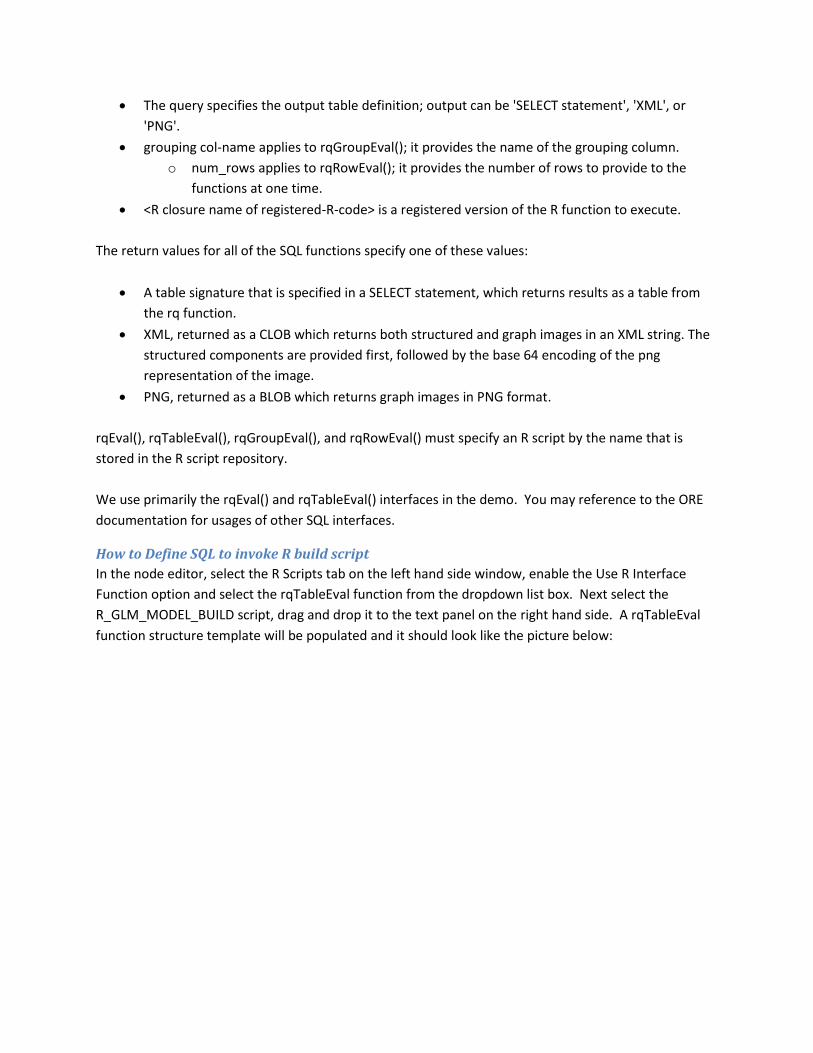
How to Define SQL to invoke R build script

In the node editor, select the R Scripts tab on the left hand side window, enable the Use R Interface

Function option and select the rqTableEval function from the dropdown list box. Next select the

R_GLM_MODEL_BUILD script, drag and drop it to the text panel on the right hand side. A rqTableEval

function structure template will be populated and it should look like the picture below:

Replace the first cursor statement with a select statement that specifies the input data. Select the

Source tab on the left hand side window, and then expand the input node Build Data Split_N$10129 to

show all available columns. Next select all columns except the CUSTOMER_ID column (case id should

not used for R model build), drag and drop all columns to the text panel to replace the wild card * in the

cursor select statement, and then replace the <table-1> with the input node Build Data Split_N$10129.

The new query should look like the picture below:

Replace the second cursor select statement with a select statement that specifies the R script

arguments. You can open the R script viewer to examine the signature of a script.

This script takes the following input arguments: dat (input data), target column (targetcolumn), model

name (modelname), and a kernel setting (family). Replace the second cursor select statement with the

following select statement that specifies the input arguments:

select

'LTV' as "targetcolumn",

'GLM_MODEL' as "modelname",

'gaussian' as "family",

1 as "ore.connect"

from dual

Note: the dat argument implicitly receives data specified by the first cursor select statement in the rq

function.

The new query should look like the picture below:

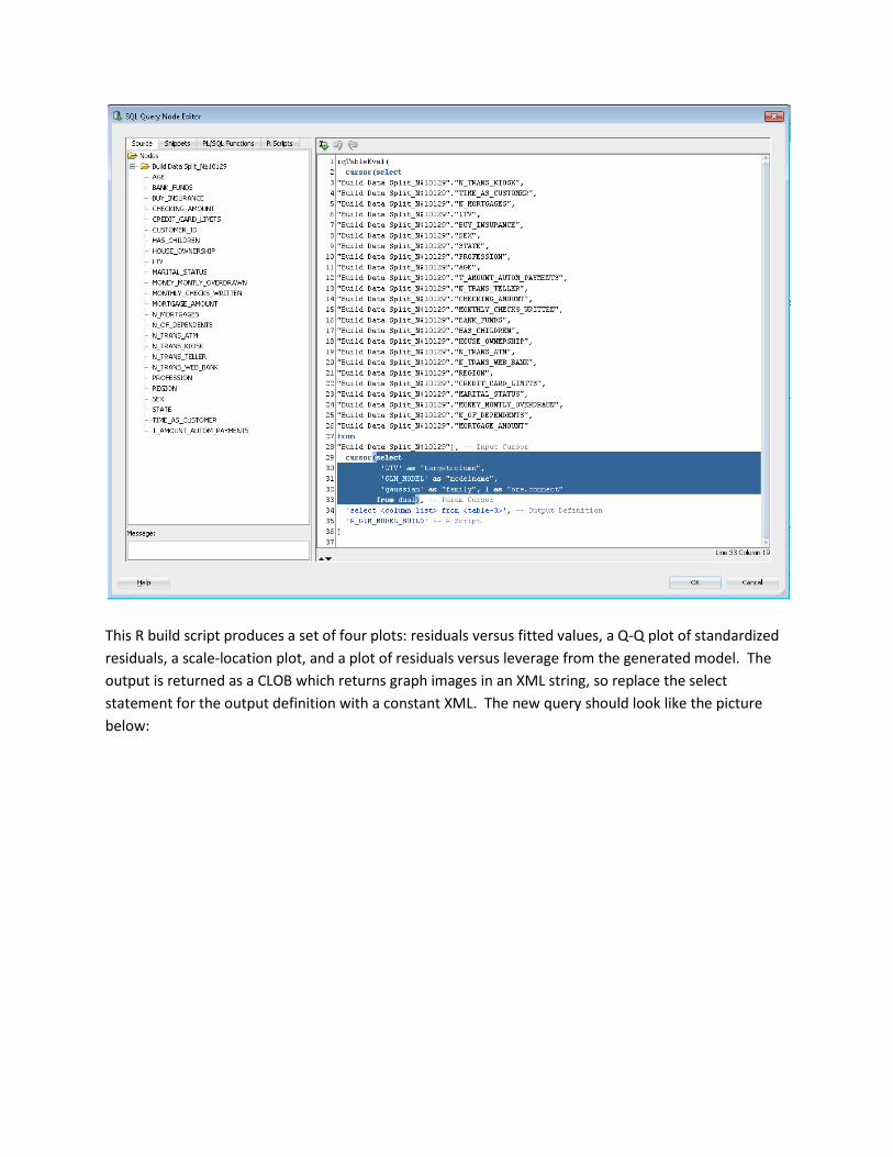
This R build script produces a set of four plots: residuals versus fitted values, a Q-Q plot of standardized

residuals, a scale-location plot, and a plot of residuals versus leverage from the generated model. The

output is returned as a CLOB which returns graph images in an XML string, so replace the select

statement for the output definition with a constant XML. The new query should look like the picture

below:

The rqTableEval function returns a table structure with a CLOB data (XML string), so add the SELECT

VALUE FROM TABLE structure in front of the query to complete the definition. The final query should

look like the picture below:

View Model Result

After the model is built, we can examine the model result in the Data viewer. Right-click on the Build

and View GLM node and select View Data from the menu to bring up the Data viewer.

The viewer shows the CLOB model result, which contains a set of four graph images (encoded in base64

string) in an XML string. To drill down to the images, double click the CLOB cell data to bring up the

View Value viewer. The viewer searches for the set of base64 encoded graph images and decodes them

to their PNG images and then displays the images individually in separate Graph tabs. The Data tab

shows the returning XML string minus the encoded base64 graph data.

The R script for rpart model build returns summary model details without any graph images, so the Data

viewer only shows XML string that contains the model summary data.

Model Comparison

For model comparison, we compare models based on computed test metrics (root mean square error

and mean absolute error) and by using residual plots. The SQL Query node, Compare Model Spec, is

used to combine the test metrics of both models into a single result set. The Create Table node,

Compare Model Result, persists the result set to a table for viewing. The SQL Query node, Compare

Residuals Spec, is used to combine the generated residual data of both models into a single result set for

graphing. The Graph node, Compare Residual Plot, is used to graph the residual plots of both models.

In the R GLM Test Metrics Spec node, we use the R script, R_REGRESS_TEST_METRICS, to compute the

test metrics of the glm model. The script takes a model name as input argument and returns the result

in a R data frame object. This data frame object is mapped to a database table by the rqEval function.

Notice we use the rqEval function to invoke the R script because no input data is passed to the script,

the test metrics are computed using the model data only. The output signature of the function is

defined as

select 1 as “Root Mean Square Err”, 1 as “Mean Absolute Err” from dual

which means the output table contains two columns, “Root Mean Square Err” and “Mean Absolute Err”,

both are numerical data type.

In the R GLM Residual Data Spec node, we use the R script, R_RESIDUAL_DATA, to compute the residual

data of the glm model. The script takes a model name as input argument and returns the result in a R

data frame object. This data frame object is mapped to a database table by the rqEval function. Notice

we use the rqEval function to invoke the R script because no input data is passed to the script, residual

data are computed using the model data only. The output signature of the function is defined as

select 1 as “PREDICTION”, 1 as “RESIDUAL” from dual

which means the output table contains two columns, “PREDICTION” and “RESIDUAL”, both are

numerical data type.

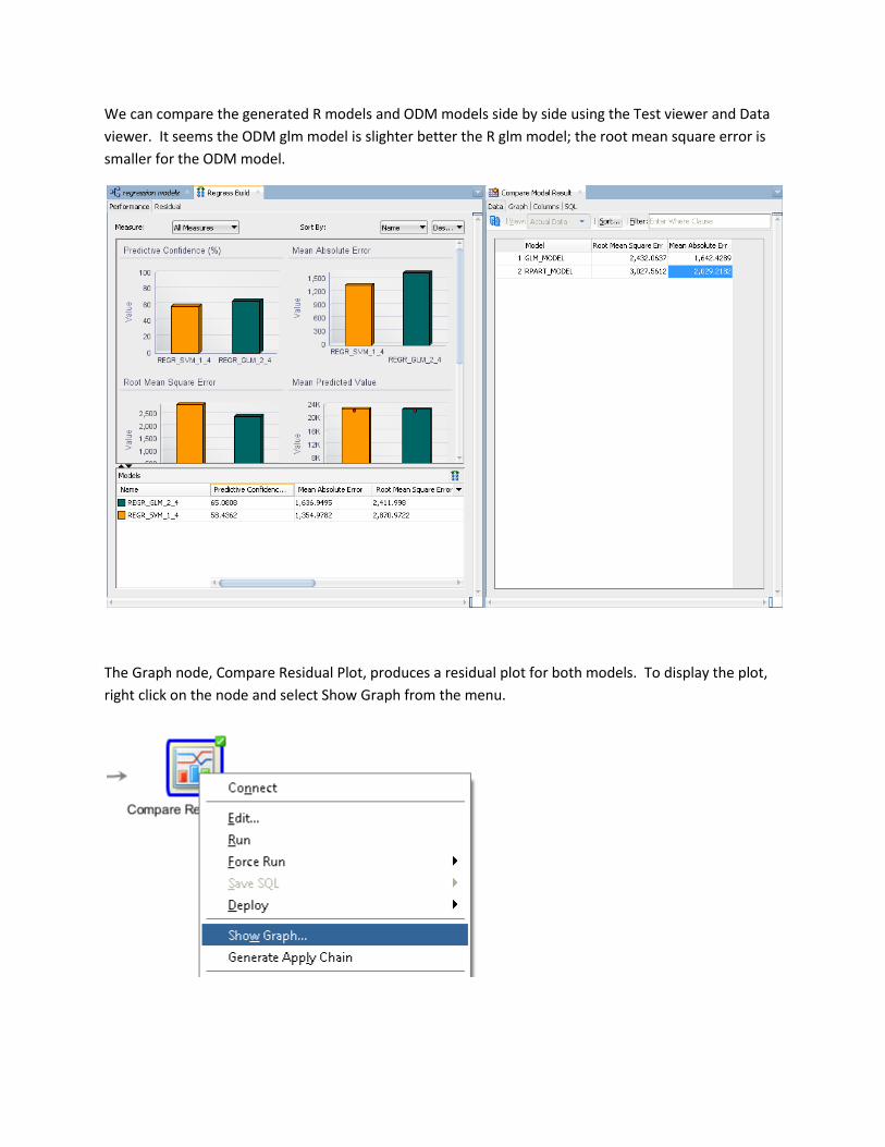
We can compare the generated R models and ODM models side by side using the Test viewer and Data

viewer. It seems the ODM glm model is slighter better the R glm model; the root mean square error is

smaller for the ODM model.

The Graph node, Compare Residual Plot, produces a residual plot for both models. To display the plot,

right click on the node and select Show Graph from the menu.

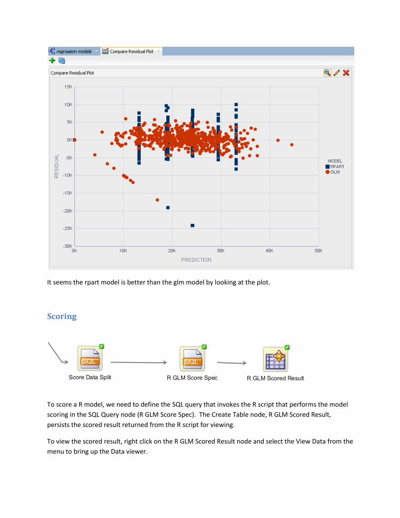
It seems the rpart model is better than the glm model by looking at the plot.

Scoring

To score a R model, we need to define the SQL query that invokes the R script that performs the model

scoring in the SQL Query node (R GLM Score Spec). The Create Table node, R GLM Scored Result,

persists the scored result returned from the R script for viewing.

To view the scored result, right click on the R GLM Scored Result node and select the View Data from the

menu to bring up the Data viewer.

Notice the result table contains a new PREDICTION column, which is generated by the R script.

Deploying the Workflow

Now that we have a successfully run workflow, we could use the new SQL script generation feature in

the Data Miner 4.0 to generate a script for the model builds. This script allows user to recreate all the

objects generated by above workflow in the target/production system. The ORE and Data Miner

Repository must be installed in the target/production system.

Conclusions The demo shows how easy it is to integrate R algorithms into the workflow using the SQL Query node.

The generated model and test results can be viewed using the generic Data viewer. The R scripts

demonstrated are for mining operations, but other type of R scripts can be used as well. For example,

user may use R scripts for statistical computation or advanced graphing. Those scripts can be easily

integrated into the workflow in similar fashion. Potentially, users can extend the workflow to include

any R operations that provided by the extensive CRAN packages or use his own scripts.

References Oracle R Enterprise: http://www.oracle.com/technetwork/database/options/advanced-analytics/r-

enterprise/index.html?ssSourceSiteId=ocomen