Optimum design for artiﬁcial neural networks: an example ... · Optimum design for artiﬁcial...

Optimum design for arti®cial neural networks: an example in abicycle derailleur system

T.Y. Lin, C.H. Tseng*

Department of Mechanical Engineering, National Chiao Tung University, Hsinchu 30050, Taiwan

Received 1 June 1998; accepted 1 September 1999

Abstract

The integration of neural networks and optimization provides a tool for designing network parameters and improvingnetwork performance. In this paper, the Taguchi method and the Design of Experiment (DOE) methodology are used tooptimize network parameters. The users have to recognize the application problems and choose a suitable Arti®cial Neural

Network model. Optimization problems can then be de®ned according to the model. The Taguchi method is ®rst applied to aproblem to ®nd out the more important factors, then the DOE methodology is used for further analysis and forecasting. ALearning Vector Quantization example is shown for an application to bicycle derailleur systems. # 2000 Elsevier Science Ltd.All rights reserved.

Keywords: Neural networks; Optimization; Taguchi method; Design of experiments; Bicycle derailleur systems

1. Introduction

Arti®cial Neural Networks (ANNs) are receivingmuch attention currently because of their wide applica-bility in research, medicine, business, and engineering.ANNs provide better and more reasonable solutionsfor many problems that either can or cannot be solvedby conventional technologies. Especially in engineeringapplications, ANNs o�er improved performance inareas such as pattern recognition, signal processing,control, forecasting, etc.

In the past few years, many ANN models withdi�erent strengths have been introduced for variousapplications. According to the di�erent ANN modelsused, many training algorithms have been developedto improve the accuracy and convergence of themodels. Although a lot of research is being concen-

trated in these two ®elds, there is still a conventionalproblem in ANN design. Users have to choose thearchitecture and determine many of the parameters ina selected network. For instance, in a ``MultilayerFeedforward (MLFF) Neural Network'', the architec-ture, such as the number of layers and the number ofunits in each layer, has to be determined. If a``Backpropagation with Momentum'' training algor-ithm is selected, many parameters, such as the learningrate, momentum term, weight initialization range, etc.,have to be selected. It is not easy for a user to choosea suitable network even if he is an experienceddesigner. The ``trial-and-error'' technique is the usualway to get a better combination of network architec-ture and parameters.

Therefore, there must be an easier and more e�cientway to overcome this disadvantage. Especially in en-gineering applications, an engineer, with or without anANN background, should not spend so much time inoptimizing the network. In recent years, the Taguchimethod (Taguchi, 1986; Peace, 1993) has become anew approach that can be used for solving the optimiz-

Engineering Applications of Arti®cial Intelligence 13 (2000) 3±14

0952-1976/00/$ - see front matter # 2000 Elsevier Science Ltd. All rights reserved.

PII: S0952-1976(99 )00045 -7

www.elsevier.com/locate/engappai

* Corresponding author. Tel.: +886-35-712-121; fax: +886-35-720-

634.

E-mail address: [email protected] (C.H. Tseng).

ation problems in this ®eld. The parameters and archi-tectures of an MLFF network were selected by usingthe Taguchi method in Khaw et al. (1995). This canimprove the original network design to obtain a betterperformance. The same technique has been used tooptimize Neocognitron Networks (Teo and Sim, 1995)and another MLFF network (Lin and Tseng, 1998).The Taguchi Method is a type of optimization tech-nique, which is very well suited to solving problemswith continuous, discrete and qualitative design vari-ables. Therefore, any ANN model can be optimized bythis method. Another method, the genetic algorithm,which requires a large computational cost, has beenapplied to populations of descriptions of networks inorder to learn the most appropriate architecture(Miller et al., 1989).

In this study, a systematic process is introduced toobtain the optimum design of a neural network. TheTaguchi method and the Design of Experiments tech-nique (DOE) (Montgomery, 1991) are the main tech-niques used. Unlike previous studies, the Taguchimethod is used here to simplify the optimization pro-blems. Then, DOE is more easily performed. Becauseof the stronger statistical basis of DOE methodologies,many analyses can be executed. Finally, a LearningVector Quantization (LVQ) network is demonstratedas an example. The method proposed in this paper canalso be applied to any ANN model. The integration ofoptimization and ANNs in this paper was simulatedby a computer program which can be executed auto-matically and easily.

2. Optimization process

Optimization techniques are used to obtain animproved solution under given circumstances. In ANNdesign, it helpful to improve the original settings of anetwork in order to get a better performance. For theconvenience of further analysis, the parameters inANNs must be classi®ed as follows.

2.1. Design parameter classi®cation

ANNs are de®ned by a set of quantities, some ofwhich are viewed as variables during the design pro-cess. These parameters are classi®ed into three partsaccording to the numerical quantities. For an n-vectorx��x1, x2, . . ., xn�, there are

1. Continuous design parameters:

xklRxkRxku k � 1, 2, . . . , n �1�where xk 2 Rn, xkl is the lower bound of xk, xku isthe upper bound of xk:

2. Discrete design parameters: xk 2 �xk1, xk2, . . ., xkm�and m is the size of the discrete set.

3. Qualitative design parameter: xk is a qualitative vari-able which cannot be described by a numerical ex-pression.

For example, consider an MLFF neural networkwith a ``backpropagation with momentum'' trainingmethod. The continuous design parameters are thelearning rate, momentum term and weight initializa-tion range. The discrete design parameters are thenumber of hidden layers, the number of units ineach layer and the number of training data items.The qualitative design parameters are the activationfunction type, the network typologies and the nu-merical method, such as the gradient descent, conju-gate gradient and BFGS (Arora, 1989).

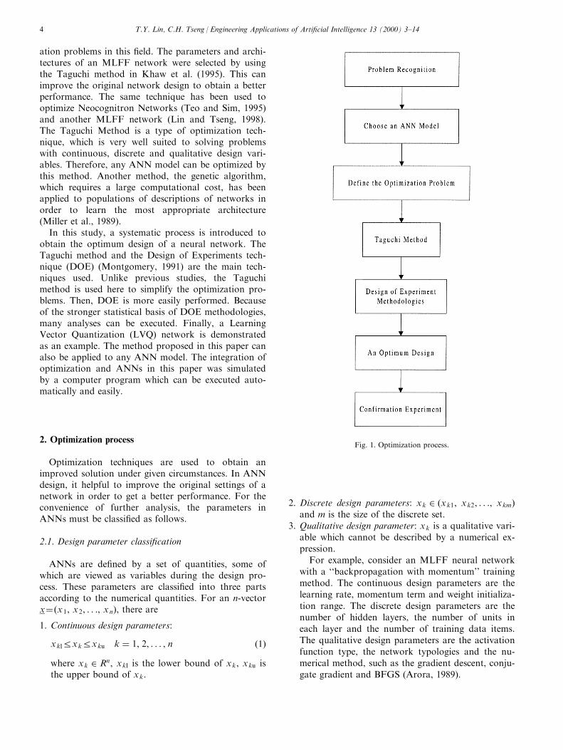
Fig. 1. Optimization process.

T.Y. Lin, C.H. Tseng / Engineering Applications of Arti®cial Intelligence 13 (2000) 3±144

2.2. Optimization problem

In order to obtain an optimum design for a neuralnetwork, an optimization process is proposed in Fig.1. First, choose a suitable ANN model for the appli-cation. The optimization problem can be formulatedas follows.

Find an n-vector x� �x1, x2, . . ., xn� of design vari-ables to minimize a vector objective function

F�x� ��f1�x�, f2�x�, . . . , fq�x�

� �2�

subject to the constraints.

hj�x� � 0; j � 1, 2, . . . , p

gi�x�R0; i � 1, 2, . . . , m: �3�The design variables x can be classi®ed into threeparts: continuous, discrete and qualitative design vari-ables, as de®ned above. The objective functions rep-resent some criteria that are used to evaluate di�erentdesigns. In ANN design, the objective function can bethe training error, the learning e�ciency, the groupingerror, etc. For engineering design problems, there aresome limitations, called constraints, and design vari-ables are not completely freely selected. Equality aswell as inequality constraints often exist in a problem.

2.3. Traditional optimization method

Numerical methods, such as Sequential LinearProgramming (SLP) and Sequential QuadraticProgramming (SQP) (Arora, 1989), which areemployed to solve optimization problems, are usuallyreferred to as ``traditional methods''. In ANN design,it is not appropriate to use these schemes to solve pro-blems. The reasons can be stated as follows.

1. There exist qualitative design parameters and thesequalitative design parameters cannot be describedby a numerical expression. Therefore, they cannotbe solved using numerical methods.

2. There exist non-pseudo-discrete design parameters.These discrete parameters, which occur when thesolution to a continuous problem is perfectly mean-ingful but cannot be accepted due to extraneousrestrictions, are termed as ``pseudo-discrete par-ameters'' which can be solved by traditionalmethods (Gill et al., 1981). For instance, the vari-able in a design problem could be the diameter of apipe. The diameter is a continuous variable, butonly speci®c values, such as 1 in, 1.5 in and 2 in,can be found in the market. This kind of variable iscalled a ``pseudo-discrete'' design parameter. Manynon-pseudo-discrete parameters that are intrinsically

discrete, such as the number of units and layers,have to be determined in ANN design.

3. The objective function is complicated. In applyingthe traditional methods, ®rst order or second orderdi�erentials of the objective function have to bechecked before using SLP or SQP. However, inANN design, it is di�cult or impossible to write thenumerical expressions of the objective function. Forexample, the grouping error is treated as the objec-tive function, but the grouping error of every train-ing process may be calculated from software or auser subroutine, which is seen as a ``black box''.Therefore, only the implicit form of the objectivefunction can be obtained. There is no explicit formof the objective function for checking.

For the above reasons, traditional optimizationmethods cannot be performed well in ANN design. Onthe other hand, there are no such limitations when

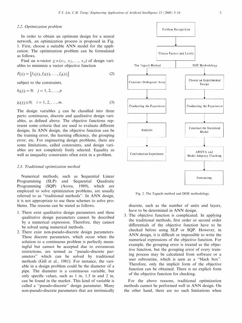
Fig. 2. The Taguchi method and DOE methodology.

T.Y. Lin, C.H. Tseng / Engineering Applications of Arti®cial Intelligence 13 (2000) 3±14 5

using other kinds of optimization methods, such as theTaguchi method and DOE methodology.

2.4. The Taguchi method

Dr. Genichi Taguchi's methods were developed afterWorld War II in Japan. His most notable contri-butions lie in quality improvement, but in recent years,the basic concepts of the Taguchi method has beenwidely applied in solving optimization problems, es-pecially in zero order problems. Because the Taguchimethod is a kind of fractional factorial DOE, thesimulation or experiment at times can be reduced,compared to DOE. For example, if there are seventwo-level factors in a design problem, only eight simu-lations have to be done in the Taguchi method. InDOE, however there are 27 � 128 simulations thathave to be done.

Fig. 2 shows the process of the Taguchi method.The engineers must recognize the application problemwell and choose a suitable ANN model. In the selectedmodel, the design parameters (factors) which need tobe optimized have to be determined. Using orthogonalarrays, simulations can be executed in a systematicway. From simulation results, the responses can beanalyzed by level average analysis and signal-to-noise(S/N ) ratio in the Taguchi method (Taguchi, 1986).

2.5. DOE methodology

DOE is a test or series of tests in which the designermay observe and identify the reasons for changes in

the output response from the changes in the input par-ameters. Fig. 2 also shows the process of DOE. Unlikethe Taguchi method, a statistical model is constructedfor the simulations and the experiment. Therefore,some assumptions and validations of the model (modeladequacy checking) have to be made, both before andafter the experiment. The experimental strategy is tochange one parameter and keep the rest of the par-ameters constant in each step. Therefore, the exper-iment and simulation times are much longer than inthe Taguchi method as mentioned before. The exper-imental response, such as the training error and con-vergence speed, can be analyzed and forecast by``Analysis of Variance'' (ANOVA) and other statisticaltechniques (Montgomery, 1991).

2.6. The Taguchi method vs. DOE methodology

In the optimization process shown in Fig. 1, theTaguchi method is treated as a pre-running of the de-sign parameters. For some engineering applications, itis quite su�cient to use the Taguchi method. There aremany reasons to do so. In design problems, there aresometimes a large number of design parameters. It isnot e�cient to use DOE methodologies at this timebecause of too many training cases. Therefore, theTaguchi method is used to reduce the training cases,and to ®nd the more important parameters that a�ectthe response of the neural network. Afterwards, theDOE methodology can be easily completed using asmaller number of important parameters, keeping

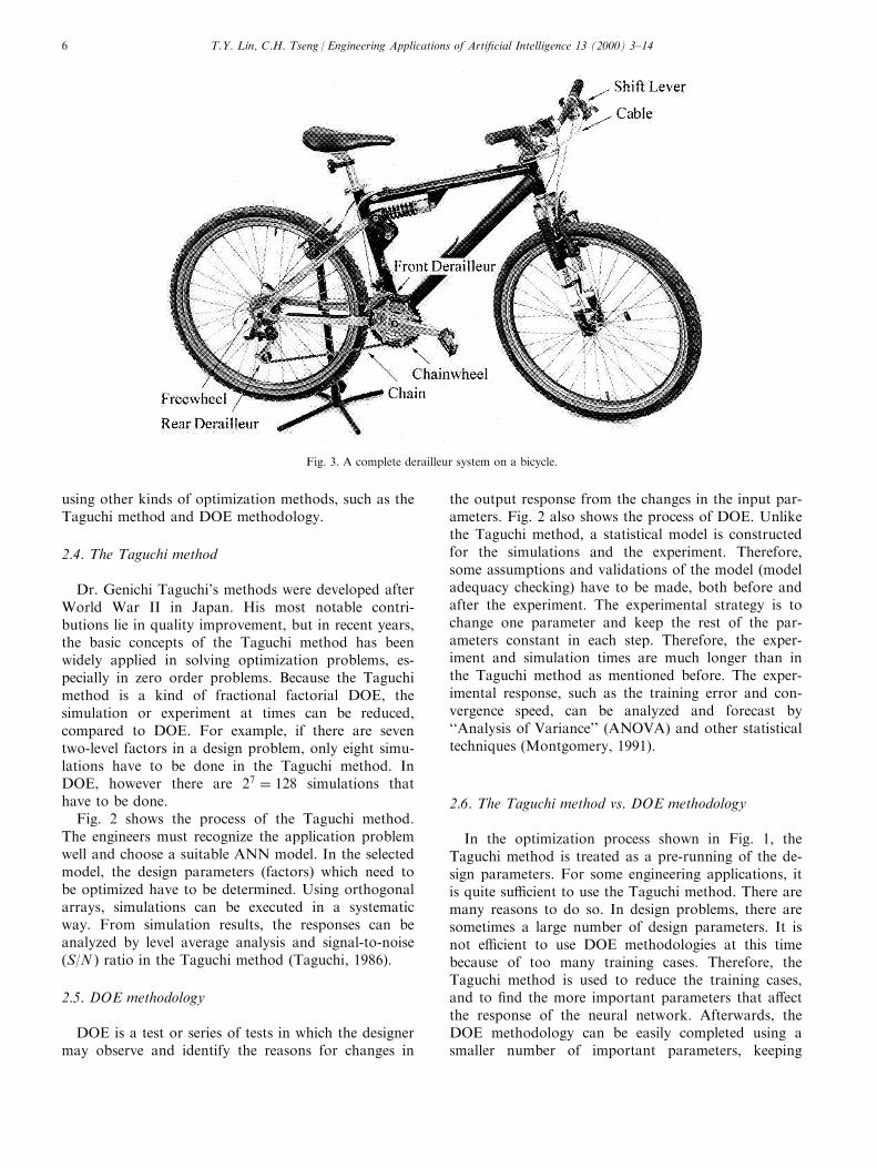
Fig. 3. A complete derailleur system on a bicycle.


other parameters constant from the conclusions of theTaguchi method.

In the DOE methodology, the experimental matrixcontains all the combinations of factors and levels.Therefore, the experimental data are su�cient to con-struct the statistical models for the analytical phase.Because of the stronger statistical base in DOE meth-odology, ANOVA can be executed in DOE but it can-not be executed in the Taguchi method. ANOVAprovides the sensitivity analysis in DOE, and thecharacteristics of the parameters can be realized. Also,a forecast can be made to ®nd the optimal combi-nations of the design parameters. The process of usingDOE and the Taguchi method is described inAppendix A.

3. The LVQ example: part 1

In order to demonstrate the optimum design pro-cesses, an application with a Learning VectorQuantization (LVQ) model is shown. In this example,the purpose is to distinguish the type of chain engage-ment to be used in the rear derailleur system of abicycle.

3.1. Problem description

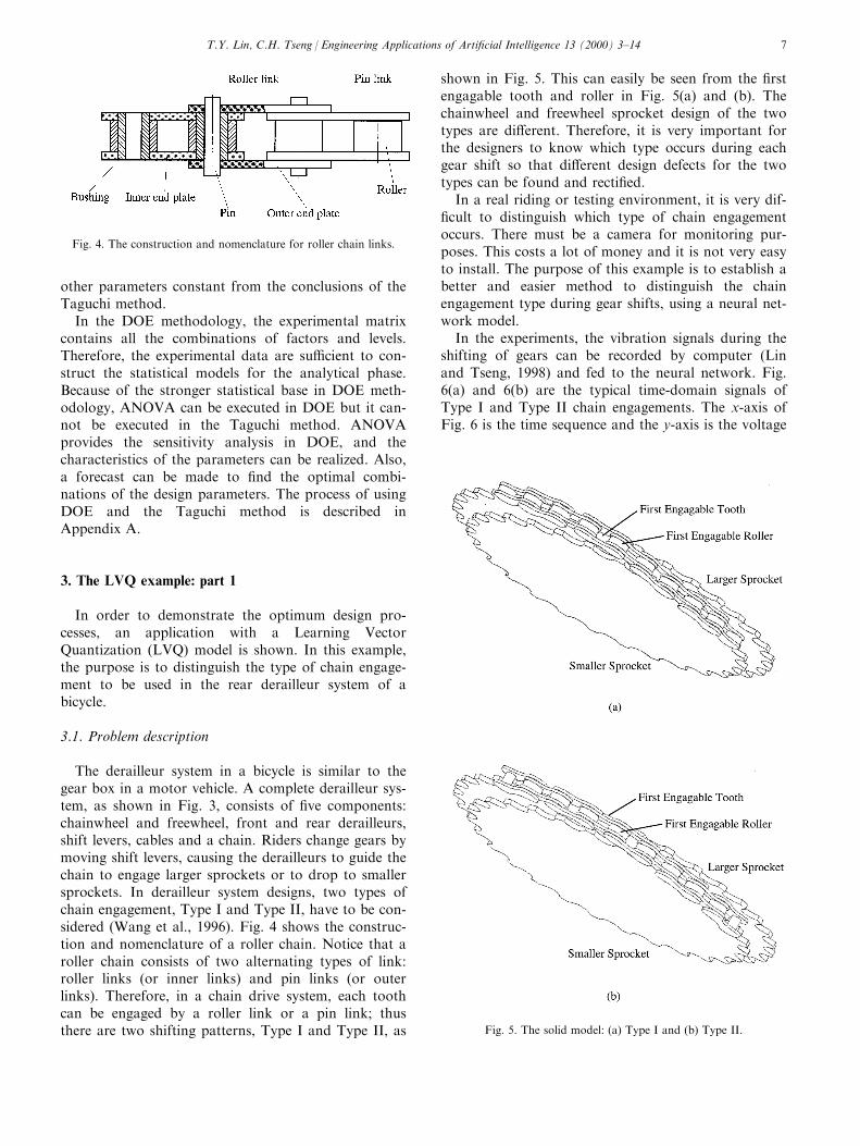
The derailleur system in a bicycle is similar to thegear box in a motor vehicle. A complete derailleur sys-tem, as shown in Fig. 3, consists of ®ve components:chainwheel and freewheel, front and rear derailleurs,shift levers, cables and a chain. Riders change gears bymoving shift levers, causing the derailleurs to guide thechain to engage larger sprockets or to drop to smallersprockets. In derailleur system designs, two types ofchain engagement, Type I and Type II, have to be con-sidered (Wang et al., 1996). Fig. 4 shows the construc-tion and nomenclature of a roller chain. Notice that aroller chain consists of two alternating types of link:roller links (or inner links) and pin links (or outerlinks). Therefore, in a chain drive system, each toothcan be engaged by a roller link or a pin link; thusthere are two shifting patterns, Type I and Type II, as

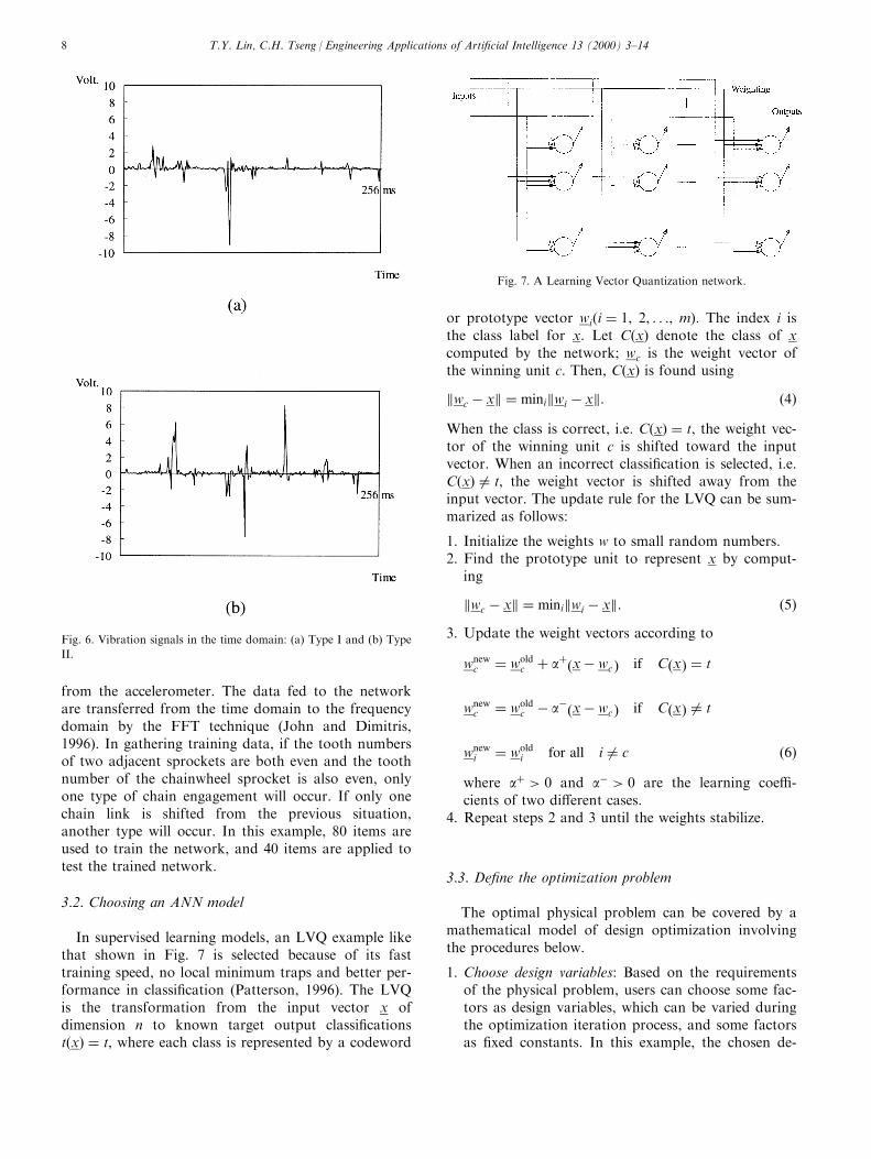
shown in Fig. 5. This can easily be seen from the ®rstengagable tooth and roller in Fig. 5(a) and (b). Thechainwheel and freewheel sprocket design of the twotypes are di�erent. Therefore, it is very important forthe designers to know which type occurs during eachgear shift so that di�erent design defects for the twotypes can be found and recti®ed.

In a real riding or testing environment, it is very dif-®cult to distinguish which type of chain engagementoccurs. There must be a camera for monitoring pur-poses. This costs a lot of money and it is not very easyto install. The purpose of this example is to establish abetter and easier method to distinguish the chainengagement type during gear shifts, using a neural net-work model.

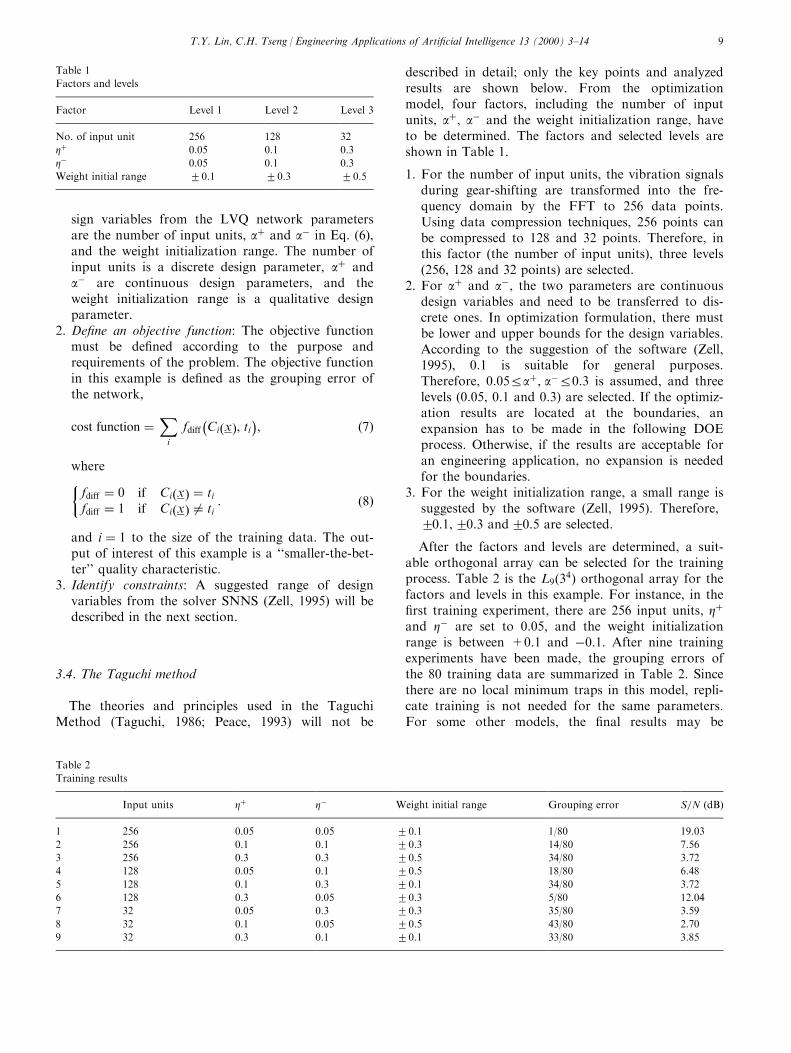
In the experiments, the vibration signals during theshifting of gears can be recorded by computer (Linand Tseng, 1998) and fed to the neural network. Fig.6(a) and 6(b) are the typical time-domain signals ofType I and Type II chain engagements. The x-axis ofFig. 6 is the time sequence and the y-axis is the voltage

Fig. 4. The construction and nomenclature for roller chain links.

Fig. 5. The solid model: (a) Type I and (b) Type II.


from the accelerometer. The data fed to the networkare transferred from the time domain to the frequencydomain by the FFT technique (John and Dimitris,1996). In gathering training data, if the tooth numbersof two adjacent sprockets are both even and the toothnumber of the chainwheel sprocket is also even, onlyone type of chain engagement will occur. If only onechain link is shifted from the previous situation,another type will occur. In this example, 80 items areused to train the network, and 40 items are applied totest the trained network.

3.2. Choosing an ANN model

In supervised learning models, an LVQ example likethat shown in Fig. 7 is selected because of its fasttraining speed, no local minimum traps and better per-formance in classi®cation (Patterson, 1996). The LVQis the transformation from the input vector x ofdimension n to known target output classi®cationst�x� � t, where each class is represented by a codeword

or prototype vector wi�i � 1, 2, . . ., m�: The index i isthe class label for x: Let C�x� denote the class of xcomputed by the network; wc is the weight vector ofthe winning unit c. Then, C�x� is found using

kwc ÿ xk � minikwi ÿ xk: �4�When the class is correct, i.e. C�x� � t, the weight vec-tor of the winning unit c is shifted toward the inputvector. When an incorrect classi®cation is selected, i.e.C�x� 6� t, the weight vector is shifted away from theinput vector. The update rule for the LVQ can be sum-marized as follows:

1. Initialize the weights w to small random numbers.2. Find the prototype unit to represent x by comput-

ing

kwc ÿ xk � minikwi ÿ xk: �5�3. Update the weight vectors according to

wnewc � wold

c � a��xÿ wc � if C�x� � t

wnewc � wold

c ÿ aÿ�xÿ wc � if C�x� 6� t

wnewi � wold

i for all i 6� c �6�where a� > 0 and aÿ > 0 are the learning coe�-cients of two di�erent cases.

4. Repeat steps 2 and 3 until the weights stabilize.

3.3. De®ne the optimization problem

The optimal physical problem can be covered by amathematical model of design optimization involvingthe procedures below.

1. Choose design variables: Based on the requirementsof the physical problem, users can choose some fac-tors as design variables, which can be varied duringthe optimization iteration process, and some factorsas ®xed constants. In this example, the chosen de-

Fig. 6. Vibration signals in the time domain: (a) Type I and (b) Type

II.

Fig. 7. A Learning Vector Quantization network.


sign variables from the LVQ network parametersare the number of input units, a� and aÿ in Eq. (6),and the weight initialization range. The number ofinput units is a discrete design parameter, a� andaÿ are continuous design parameters, and theweight initialization range is a qualitative designparameter.

2. De®ne an objective function: The objective functionmust be de®ned according to the purpose andrequirements of the problem. The objective functionin this example is de®ned as the grouping error ofthe network,

cost function �Xi

fdiff

ÿCi�x�, ti

�, �7�

where�fdiff � 0 if Ci�x� � tifdiff � 1 if Ci�x� 6� ti

: �8�

and i � 1 to the size of the training data. The out-put of interest of this example is a ``smaller-the-bet-ter'' quality characteristic.

3. Identify constraints: A suggested range of designvariables from the solver SNNS (Zell, 1995) will bedescribed in the next section.

3.4. The Taguchi method

The theories and principles used in the TaguchiMethod (Taguchi, 1986; Peace, 1993) will not be

described in detail; only the key points and analyzedresults are shown below. From the optimizationmodel, four factors, including the number of inputunits, a�, aÿ and the weight initialization range, haveto be determined. The factors and selected levels areshown in Table 1.

1. For the number of input units, the vibration signalsduring gear-shifting are transformed into the fre-quency domain by the FFT to 256 data points.Using data compression techniques, 256 points canbe compressed to 128 and 32 points. Therefore, inthis factor (the number of input units), three levels(256, 128 and 32 points) are selected.

2. For a� and aÿ, the two parameters are continuousdesign variables and need to be transferred to dis-crete ones. In optimization formulation, there mustbe lower and upper bounds for the design variables.According to the suggestion of the software (Zell,1995), 0.1 is suitable for general purposes.Therefore, 0:05Ra�, aÿR0:3 is assumed, and threelevels (0.05, 0.1 and 0.3) are selected. If the optimiz-ation results are located at the boundaries, anexpansion has to be made in the following DOEprocess. Otherwise, if the results are acceptable foran engineering application, no expansion is neededfor the boundaries.

3. For the weight initialization range, a small range issuggested by the software (Zell, 1995). Therefore,20.1,20.3 and20.5 are selected.

After the factors and levels are determined, a suit-able orthogonal array can be selected for the trainingprocess. Table 2 is the L9�34� orthogonal array for thefactors and levels in this example. For instance, in the®rst training experiment, there are 256 input units, Z�

and Zÿ are set to 0.05, and the weight initializationrange is between +0.1 and ÿ0.1. After nine trainingexperiments have been made, the grouping errors ofthe 80 training data are summarized in Table 2. Sincethere are no local minimum traps in this model, repli-cate training is not needed for the same parameters.For some other models, the ®nal results may be

Table 1

Factors and levels

Factor Level 1 Level 2 Level 3

No. of input unit 256 128 32

Z� 0.05 0.1 0.3

Zÿ 0.05 0.1 0.3

Weight initial range 20.1 20.3 20.5

Table 2

Training results

Input units Z� Zÿ Weight initial range Grouping error S=N (dB)

1 256 0.05 0.05 20.1 1/80 19.03

2 256 0.1 0.1 20.3 14/80 7.56

3 256 0.3 0.3 20.5 34/80 3.72

4 128 0.05 0.1 20.5 18/80 6.48

5 128 0.1 0.3 20.1 34/80 3.72

6 128 0.3 0.05 20.3 5/80 12.04

7 32 0.05 0.3 20.3 35/80 3.59

8 32 0.1 0.05 20.5 43/80 2.70

9 32 0.3 0.1 20.1 33/80 3.85


a�ected by di�erent initial designs. Therefore, repli-cated training is necessary for the following S=Nanalysis.

The last column in Table 2 is the signal-to-noiseratio �S=N). The equation for calculating the S=N for

the smaller-the-better quality characteristic is Eq. (A1).In this example, there is only one replicate, therefore,the physical meaning of S=N is similar to the groupingerrors in Table 2. The grouping errors are used hereinstead of S=N for easier understanding.

The next step in the Taguchi method is LevelAverage Analysis. The goal is to identify the strongeste�ects and to determine the combination of factorsand levels that can produce the most desired results.

Table 3 is the response table, which shows the averageexperiment result for each factor level. The total e�ectof the 256 input units is 16. This is the average group-ing error of the ®rst three rows in Table 2��1� 14� 80�=3 � 16). Other response values can becalculated by using a similar method. For the numberof input units, 256 units can get a smaller groupingerror than other levels. The same principle can be usedto make Z� and Zÿ equal to 0.05, and the weight initi-alization range to be between +0.3 and ÿ0.3. Fig. 8shows the response curves for the four factors. Itshows that the four factors do have a strong e�ect on

the grouping errors. Therefore, the recommended fac-tor levels are: 256 input units, Z� � 0:05, Zÿ � 0:05and a weight initialization range of 20:3:

4. The LVQ example: part 2

From the Taguchi method, an improved design ofthe LVQ network is obtained. Fig. 2 shows the nextstep of the optimization process Ð the DOE method-ology. The main purpose of this step is to further ana-lyse the results of the Taguchi method, and to getmore accurate settings for the factors. The DOE the-ories and principles (Montgomery, 1991) will not bedescribed here; only the key points and results areshown below.

4.1. Choosing an experimental design

For the number of input units, it is obvious that alarger number will cause smaller grouping errors inFig. 5, and that 256 units is the maximum. Therefore,the number of input units will remain at 256 in thisstep. For the weight initialization range 20:3 is notlocated at the variable boundaries and seems to be alocal minimum in Fig. 8. Therefore, this parameterwill also remain constant here. For Z� and Zÿ, theminimum response is located at the lower bound ofthe variables; therefore, an expansion of the bound-aries is required in further analysis. In summary, onlythe two continuous parameters, Z� and Zÿ, are treatedas design variables in the DOE methodology, and theother two parameters are kept constant.

The new parameter sets are shown in Table 4. Theupper and lower bounds of Z� and Zÿ are changedfrom 0.05 and 0.3 to 0.01 and 0.1. Therefore, threelevels (0.1, 0.05 and 0.01) are designed for training,while the other two parameters are kept constant.Nine training cases have to be simulated in thisexample.

4.2. Conducting the experiment

The same 80 items of training data used in theTaguchi method are also applied here. The results ofgrouping errors are also shown in Table 4. Upon com-pletion of the training experiments, DOE analysis tech-niques can be executed.

Table 3

Response table

Factor Level Error Factor Level Error

Input units 256 16 0.05 16

128 19 Zÿ 0.1 22

32 37 0.3 34

Z� 0.05 18 20.1 23

0.1 30 Weight initial range 20.3 18

0.3 34 20.5 32

Fig. 8. Response curves.

Table 4

DOE array and training results

Z�

0.1 0.05 0.01

0.1 14/80 (4.0) 26/80 (7.0) 28/80 (8.0)

Zÿ 0.05 23/80 (6.0) 1/80 (1.5) 10/80 (3.0)

0.01 29/80 (9.0) 19/80 (5.0) 1/80 (1.5)


4.3. The statistical model

This is a two-factor factorial design. The statisticalmodel of this example is

yijk � m� ti � bj � �tb�ij�eijk,8<: i � 1, 2, . . . , aj � 1, 2, . . . , bk � 1, 2, . . . , n

: �9�

where

yijk is the ijkth observation (grouping error),m is the overall mean,ti is the ith Z� e�ect (®xed e�ect),bj is the jth Zÿ e�ect (®xed e�ect),�tb�ij is the interaction between Z� and Zÿ,eijk is the random error component. eijk0NID �0,s2�:

There are three levels in each factor and only onereplicate is done; therefore, a � 3, b � 3 and k � 1:With only one replicate, there are no error estimations.One approach applied to the following analysis is toassume a negligible higher order interaction betweenZ� and Zÿ combined with an error degree of freedom.

4.4. Analysis of variance (ANOVA)

Using the statistical model and the training results,the ANOVA technique can be executed. Table 5 is theANOVA table from the SAS software, and the errorestimation is taken from the interaction between Z�

and Zÿ: If a 95 percent con®dence interval is assumed(i.e., a � 0:05, the normal setting for applications),Fa; n1; n2 � F0:05; 2; 2 � 19:0: For the null hypotheses ofti � 0 and bj � 0,

F0, Z� � 0:42 < F0:05, 2, 2 � 19:0 and

F0, Zÿ � 0:61 < F0:05, 2, 2 � 19:0:

Therefore, the null hypotheses are accepted. The con-clusion is that there is no signi®cant di�erence betweenthe three levels of Z� and Zÿ: The results can also beobserved from the Pr value in the ANOVA table.Pr � 0:68 and Pr � 0:59 mean that the probability ofrejecting null hypotheses is very high (compared to0.05). The sensitivity of Z� and Zÿ to grouping errors

is not very high. In some cases, the conclusion may bedrawn that there are signi®cant di�erences between thelevels. This means that the factor is very sensitive tothe output response.

4.5. Model adequacy checking

In the statistical model of this problem, threeassumptions are made: normality, independence andequal variance. Some tests have to be executed to ver-ify these assumptions. For checking the normality, theKruskal±Wallis Test (Montgomery, 1991) is used. InTable 4, the values in the brackets are the data ranks,Rijk, for the experiment.

S2 � 1

Nÿ 1

24Xai�1

Xbj�1

Xnk�1

R2ijk ÿ

N�N� 1�24

35� 1

8

�284:5ÿ 9� 102

4

�� 7:4375 �10�

H � 1

S2

"Xai�1

R2ijk

nÿ N�N� 1�2

4

#

� 1

55:32

�284:5ÿ 9� 102

4

�� 1:0756: �11�

Since H < w20:05, 8 � 15:51, one would accept the nullhypothesis of ti � 0 and bj � 0: There is no signi®cantdi�erence between the three levels of Z� and Zÿ: Theconclusion here is the same as that given by the usualanalysis of the variance F test. Therefore, the normal-ity assumption is justi®ed.

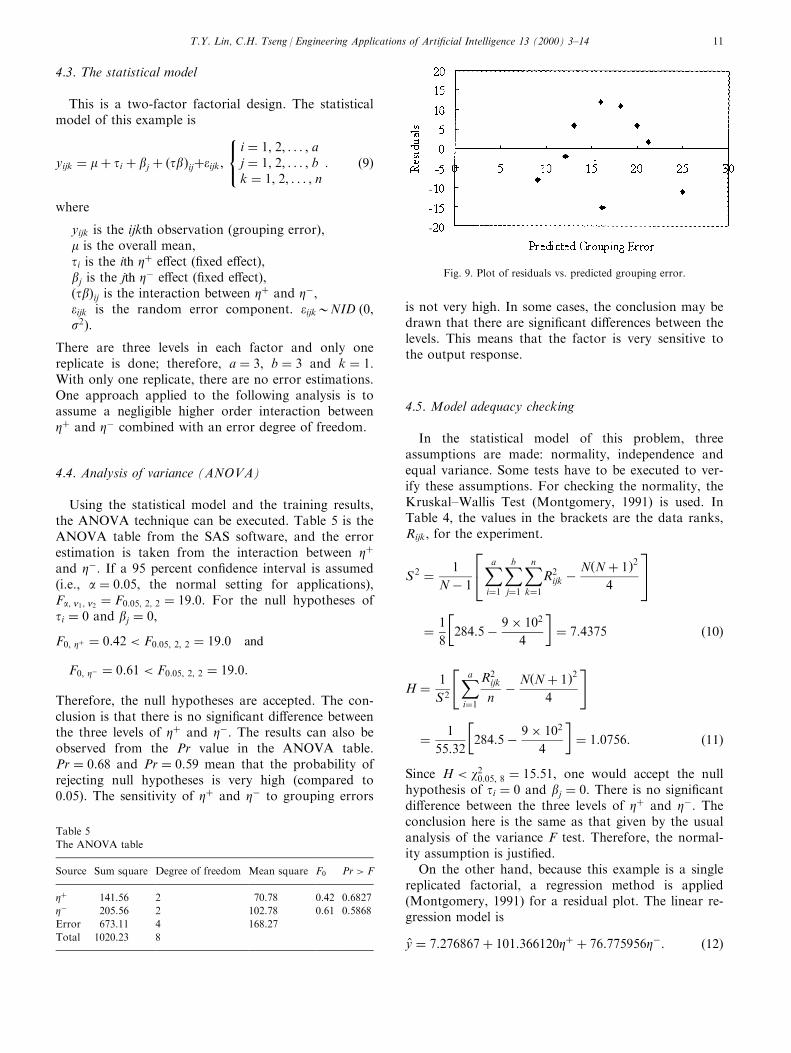
On the other hand, because this example is a singlereplicated factorial, a regression method is applied(Montgomery, 1991) for a residual plot. The linear re-gression model is

y � 7:276867� 101:366120Z� � 76:775956Zÿ: �12�

Fig. 9. Plot of residuals vs. predicted grouping error.

Table 5

The ANOVA table

Source Sum square Degree of freedom Mean square F0 Pr > F

Z� 141.56 2 70.78 0.42 0.6827

Zÿ 205.56 2 102.78 0.61 0.5868

Error 673.11 4 168.27

Total 1020.23 8


Fig. 9 plots the residuals vs. the predicted values, y,for the grouping errors. There is no obvious patternapparent, therefore, the independence and equal var-iance assumptions are justi®ed.

4.6. Forecasting

In Table 4, the training results show that two casesof Z� and Zÿ using the combination ((0.01, 0.01) and(0.05, 0.05)) will get a better grouping error. Only onegrouping error occurs among 80 training data. Inorder to get more precise results, the regressionmethod is used. Using the General Regression Modelin the SAS software (Montgomery, 1991), the highestorder Fitting Response Surface is

z � ÿ13:89� 1284:54Z� � 800:09Zÿ

ÿ 8422:84Z�2 ÿ 3867:28Zÿ

2 ÿ 68236Z�Zÿ

� 561574Z�Zÿ2 � 589352Z�

2

Zÿ

ÿ 5262346Z�2

Zÿ2

: �13�

The surface is shown in Fig. 10. Using the partialdi�erential method, the minimum z value and the cor-respondence Z� and Zÿ can be obtained: Z� � 0:046and Zÿ � 0:05:

4.7. Con®rmation experiment

Using the recommended factor levels:

number of input units: 256,Z�:0:046,Zÿ:0:05,weight initialization range: 20:3:

the grouping error after training becomes zero, i.e., allthe training data are classi®ed successfully.

5. Conclusion

Optimization techniques have been widely used inmany applications. In this paper, two major categories,the Taguchi method and the DOE methodology, areapplied to improve upon the original designs ofANNs. The users have to recognize the design problemand choose a suitable ANN model. Then, the optimiz-ation problems can be de®ned according to the model.The Taguchi method is ®rst applied to ®nd the moreimportant factors, and to simplify the design problems.DOE methodologies are then used to ®nd the sensi-tivity and a more precise combination of design par-ameters. The ®nal results of the examples introducedin this study indeed improve the initial designs and geta better performance.

Although only one ANN model, LVQ, is demon-strated in this paper, other models, such as ADALINE,MADALINE, Hop®eld Networks, MLFF, BoltzmannMachines, Recurrent Neural Networks, Neocognitrons,etc., are also suitable. Many bene®ts can be mentioned.First, this is a systematic method to use for a neural net-work design. It means that the engineer, whether or nothe or she is experienced in ANN, the Taguchi methodand DOE, can follow this process easily. Many commer-cial software packages can be applied, such as SNNS inANN and SAS in the DOE. Second, it will not take toomuch computational e�ort and time. The results of thedemonstrated examples can be obtained within 5 minwith a Pentium-150 PC. This detail was not emphasizedin this paper because it is not the major concern here.Finally, in engineering applications, it is not necessary toget a global optimization of the problems, because thattakes too much time or the algorithms may be very com-plicated. The improvement of the original designs to anacceptable region is helpful for engineers.

Acknowledgements

The support of this research by the National ScienceCouncil, Taiwan, R.O.C., under grant NSC-85-2622-E-007-012, is gratefully acknowledged.

Appendix A. The Taguchi method and DOEmethodology

Dr. Genichi Taguchi's methods were developed afterWorld War II in Japan, while the DOE methodologywas ®rst introduced by R. A. Fisher in the 1920s. TheTaguchi method is a kind of fractional factorial DOE;therefore, the simulation or experiment times can bereduced to a smaller number compared to DOE. Themost notable contributions of the methodology are inquality improvement, but in recent years, the basicFig. 10. Fitting response surface.


concepts of the Taguchi method and DOE have beenwidely applied to the solution of optimization pro-blems, especially in zero order problems. In this sec-tion, some of the basic concepts used in the Taguchimethod and DOE are described.

A.1. Problem recognition

A clear recognition of the problem often contributessubstantially to a better understanding of the phenom-ena involved, and the ®nal solution of the design pro-blem. Usually, it is necessary to convert physicalstatements or customer requirements to measurablequantities. Therefore, an optimization problem whichconsists of design variables, objective (cost) functions,and constraints can be de®ned.

A.2. Choice of factors and levels

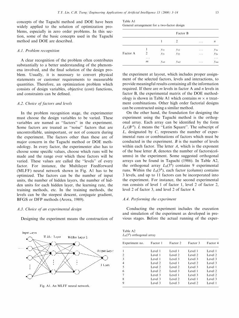
In the problem recognition stage, the experimentermust choose the design variables to be varied. Thesevariables are named as ``factors'' in the experiment.Some factors are treated as ``noise'' factors that areuncontrollable, unimportant, or not of concern duringthe experiment. The factors other than these are ofmajor concern in the Taguchi method or DOE meth-odology. In every factor, the experimenter also has tochoose some speci®c values, choose which runs will bemade and the range over which these factors will bevaried. These values are called the ``levels'' of everyfactor. For instance, the Multilayer Feedforward(MLFF) neural network shown in Fig. A1 has to beoptimized. The factors can be the number of inputunits, the number of hidden layers, the number of hid-den units for each hidden layer, the learning rate, thetraining methods, etc. In the training methods, thelevels can be the steepest descent, conjugate gradient,BFGS or DFP methods (Arora, 1989).

A.3. Choice of an experimental design

Designing the experiment means the construction of

the experiment at layout, which includes proper assign-ment of the selected factors, levels and interactions, toprovide meaningful results containing all the informationrequired. If there are m levels in factor A and n levels infactor B, the experimental matrix of the DOE method-ology is shown in Table A1 which contains m � n treat-ment combinations. Other high order factorial designscan be constructed using a similar method.

On the other hand, the foundation for designing theexperiment using the Taguchi method is the orthog-onal array. Each array can be identi®ed by the formLC�BA�: L means the ``Latin Square''. The subscript ofL, designated by C, represents the number of exper-imental runs or combinations of factors which must beconducted in the experiment. B is the number of levelswithin each factor. The letter A, which is the exponentof the base letter B, denotes the number of factors(col-umns) in the experiment. Some suggested orthogonalarrays can be found in Taguchi (1986). In Table A2,the orthogonal array L9�34� contains 9 experimentalruns. Within the L9�34�, each factor (column) contains3 levels, and up to 11 factors can be incorporated intothe experiment. For instance, the second experimentalrun consists of level 1 of factor 1, level 2 of factor 2,level 2 of factor 3, and level 2 of factor 4.

A.4. Performing the experiment

Conducting the experiment includes the executionand simulation of the experiment as developed in pre-vious stages. Before the actual running of the exper-

Table A1

General arrangement for a two-factor design

Factor B

1 2 . . . n

1 y11 y12 . . . y1nFactor A 2 y21 y22 . . . y2n

. . . . . .

m ym1 ym2 . . . ymn

Table A2

L9�34� orthogonal array

Experiment no. Factor 1 Factor 2 Factor 3 Factor 4

1 Level 1 Level 1 Level 1 Level 1








9 Level 3 Level 3 Level 2 Level 1Fig. A1. An MLFF neural network.


iment, the test plans (including the experimental order,repetition, randomization, preparation and coordi-nation) have to be developed. These preliminary e�ortsare essential and are important for smooth and e�-cient execution of the experiment.

A.5. Analysis for DOE

The analysis phase of the experiment is employed toconvert a row of data into meaningful informationand to interpret the results. The ®rst step of an analy-sis for DOE is to assume a statistical model for the ex-periment. The model contains the e�ects of the factors,their interactions, and error estimations. Threeassumptions (normality, independence and equal var-iance) are applied in the model. According to the stat-istical model, the Analysis of Variance (ANOVA) canbe accomplished using the SAS software. The ANOVAis the sensitivity analysis for the levels in each factor.Therefore, the e�ects of di�erent factors, levels, andinteractions between factors can be realized. Finally,the model adequacy checking has to be performed toprove the three assumptions in the model. For check-ing the normality, the Kruskal±Wallis Test(Montgomery, 1991) is always used. For the indepen-dence and equal variance assumptions, residual plots(Montgomery, 1991) can be used. If the model is ade-quate, the General Regression Model in the SAS soft-ware (Montgomery, 1991) can be used to forecast theoptimum combination of the experiment. The demon-stration example and the detailed descriptions of dataanalysis for DOE are shown in Section 4 of this paper.

A.6. Analysis for the Taguchi method

Dr. Taguchi recommends analyzing the mean responsefor each experiment in the orthogonal array, and analyz-ing the variation using the signal-to-noise �S=N� ratio.The S=N ratio for three di�erent objective functions are:

S

N� ÿ10 logjy

21 � y22 � . . .� y2n

nj,

for a smaller-the-better characteristic

�A1�

S

N� ÿ10 logj

1

y21� 1

y22� . . .� 1

y2nn

j,

for a larger-the-better characteristic,

�A2�

where n is the number of replicates and yn is the exper-imental response. Larger S=N values mean that strongsignals and little noise (interference) exist during the ex-periment. Therefore, larger S=N values are desired in theTaguchi Method. After the S=N calculations, the levelaverage analysis can be performed to obtain the opti-mum solution. The demonstration example and thedetailed descriptions of data analysis for the Taguchimethod are shown in Section 3 of this paper.

A.7. Con®rmatory experiment

After the analysis phase, the optimum combinationof the levels in each factor can be obtained. A con®r-matory experiment at these settings is vital for check-ing the reproducibility of the optimum combinations,and for con®rming the assumptions used in planningand designing the experiment.

References

Arora, J.S., 1989. Introduction to Optimum Design. McGraw-Hill,

New York.

Gill, P.E., Murray, W., Margaret, H.W., 1981. Practical

Optimization. Academic Press, New York.

John, G.P., Dimitris, G.M., 1996. Digital Signal Processing.

Prentice-Hall, Englewood Cli�s, NJ.

Khaw, B.S.L., John, F.C., Lennie, E.N.L., 1995. Optimum design of

neural networks using the Taguchi method. Neurocomputing 7,

225±245.

Lin, T.Y., Tseng, C.H., 1998. Using fuzzy logic and neural network

in bicycle derailleur system tests. In: Proceedings of the

International Conference on Advances in Vehicle Control and

Safety (AVCS'98), Amiens, France, 338±343.

Miller, G.F., Todd, P.M., Hedge, S.U., 1989. Designing neural net-

works using genetic algorithms. In: In: Proceedings of the Third

International Conference on Genetic Algorithms, 379±384.

Montgomery, D.C., 1991. Design and Analysis of Experiments.

Wiley, New York.

Patterson, D.W., 1996. Arti®cial Neural Networks, Theory and

Applications. Prentice-Hall, Englewood Cli�s, NJ.

Peace, G.S., 1993. Taguchi Methods, A Hands-On Approach.

Addison-Wesley, Reading, MA.

Taguchi, G., 1986. Introduction to Quality Engineering. Asian

Productivity Organization, Tokyo.

Teo, M.Y., Sim, S.K., 1995. Training the neocognitron network

using design of experiments. Arti®cial Intelligence in Engineering

9, 85±94.

Wang, C.C., Tseng, C.H., Fong, Z.H., 1996. A method for improv-

ing shifting performance. International Journal of Vehicle Design

18 (1), 100±117.

Zell, A., 1995. SNNS, Stuttgart Neural Network Simulator User

Manual, Version 4.1, Report No. 6/95. University of Stuttgart,

IPVR, Stuttgart, Germany.


Optimum design for artiﬁcial neural networks: an example ... · Optimum design for artiﬁcial...

Documents

Transcript of Optimum design for artiﬁcial neural networks: an example ... · Optimum design for artiﬁcial...