LIBRARY

OF THE

MASSACHUSETTS INSTITUTE

OF TECHNOLOGY

Digitized by the Internet Archive

in 2011 with funding from

Boston Library Consortium IVIember Libraries

http://www.archive.org/details/optimumconsumptiOOmert

Optimum Consumption and Portfolio Pvules

in a Continuous-time Model

by

Robert C. Merton

Number 58 August 1970

This paper was supported by the NationalScience Foundation (grant number GS 1812) . Theviews expressed in this paper are the author'ssole responsibility, and do not reflect thoseof the National Science Foundation, the Depart-ment of Economics, nor of the Massachusetts In-stitute of Technology.

Optimum Consumption and Portfolio Rules in a Continuous-time Model *

Robert C. Merton

M.I.T. March, 1970

1. Introduction . A common hypothesis about the

behavior of (limited liability) asset prices In perfect mar-

kets Is the random walk of returns or (In Its continuous-

time form) the "geometric Brownian motion" hypothesis which

implies that asset prices are stationary and log-normally

distributed. A number of investigators of the behavior of

stock and commodity prices have questioned the accuracy of

the hypothesis. In particular, Cootner [2] and others

have criticized the independent increments assumption, and

Osborne [2] has examined the assumption of statlonariness

.

Mandelbrolt [2] and Pama [2] argue that stock and commodity

price changes follow a stable-Paretian distribution with

infinite second-moments. The non-academic literature on

the stock market is also filled with theories of stock

price patterns and trading rules to "beat the market",

rules often called "technical analysis" or "charting",

and that presupposes a departure from random price changes.

aI would like to thank P. A. Samuelson, R.M. Solow, P. A. Diamond,J. A. Mlrrlees, J.S. Flemmlng, and D.T. Scheffman for theirhelpful discussions. Of course, all errors are mine. Aidfrom the National Science Foundation is gratefully acknowl-edged

^1^

For a number of Interesting papers on the subject, seeCootner [2]. An excellent survey article is "EfficientCapital Markets :A Review of Theory and Empirical VJork"(a draft), E.F. Fama, November, 1969.

536357

-2-

In an earlier paper [12], I examined the continuous-

time consumption-portfolio problem for an Individual whose

Income Is generated by capital gains on Investments In

assets with prices assumed to satisfy the "geometric

Brownlan motion" hypothesis. I.e. I studied Max eJ U(C,t)dt

where U Is the Instantaneous utility function; C is consump-

tion; E is the expectation operator. Under the additional

assumption of a constant relative or constant absolute risk-

aversion utility function, explicit solutions for the opti-

mal consumption and portfolio rules were derived. The

changes in these optimal rules with respect to shifts in

various parameters such as expected return. Interest rates,

and risk were examined by the technique of comparative

statics.

The present paper extends these results for more gen-

eral utility functions, price behavior assumptions, and

for Income generated also from non-capital gains sources.

It is shown that if the "geometric Brownlan motion" hy-

pothesis is accepted, then a general "Separation" or "mutual

fund" theorem can be proved such that, in this model, the

classical Tobln mean-variance rules hold without the ob-

jectionable assumptions of quadratic utility or of normality

of distributions for prices. Hence, when asset prices are

generated by a geometric Brownlan motion, one can work with

the two-asset case without loss of generality-. If the fur-

ther assumption is made that the utility function of the

individual is a member of the family of utility functions

called the "HARA" family, explicit solutions for the opti-

mal consumption and portfolio rules are derived and a num-

ber of theorems proved. In the last parts of the paper,

the effects on the consumption and portfolio rules of al-

ternative asset price dynamics, in which changes are neither

stationary nor independent, are examined along with the

effects of Introducing wage income, uncertainty of life

ejcpectancy, and the possibility of default on (formerly)

"risk-free" assets.

-3-

2. A digression on It6 Processes . To apply the

dynamic programming technique in a continuous-time model,

the state variable dynamics must be expressible as Markov

stochastic processes defined over time intervals of length

h, no matter how small h is. Such processes are referred

to as infinitely divisible in time. The two processes of

this type are: functions of Gauss-Wiener Brownian

motions which are continuous in the "space" variables and

functions of Polsson processes which are discrete in the

space variables. Because neither of these processes is

differentiable in the usual sense, a more general type of

differential equation must be developed to express the

dynamics of such processes. A particular class of contin-

uous-time Markov processes of the first type called Ito

Processes are defined as the solution to the stochastic

differential equation

(1) dP <= f(P,t)dt + g(P,t)dz

where P, f , and g are n-vectors and z(t) is a n-vector of

I ignore those infinitely divisible processes with in-finite moments which include those members of the stableParetian family other than the normal.

Ito Processes are a special case of a more general classof stochastic processes called Strong diffusion processes(see Kushner [9], p. 22).(1) is a short-hand expression for the stochastic integral

t t

P(t) = P(o) + ^ f(P,s)ds + ^ g(P,s)dz

where P(t) is the solution to (1) with probability one.A rigorous discussion of the meaning of a solution

to equations like (1) is not presented here. Only thosetheorems needed for formal manipulation and solution ofstochastic differential equations are in the text andthese without proof. For a complete discussion of ItoProcesses, see the seminal paper of Ito [7], Ito andMcKean [8], and McKean [11]. For a short descriptionand some proofs, see Kushner [9]j p. 12-18. For a heuristicdiscussion of continuous-time Markov processes in general,see Cox and Miller [3]j chapter 5.

-4-

standard normal random variables. Then dz(t) is called a

multl-dimenslonal Wiener process (or Brownian motion).

The fundamental tool for formal manipulation and solu-

tion of stochastic processes of the Ito type is Ito's Lemma

stated as follows

Lemma: Let F(Pi , . . . jP^^ jt ) be a C^ func-

tion defined on R X[o,°°) and take the

stochastic integrals

P^(t) = P^(o) + /^ fj_(P,s)ds + ^^ g^(P,s)dz^,

i = 1,. ..,n;

then the time-dependent random variable

Y = F is a stochastic integral and its

stochastic differential Is

« - 2? % ^^1 ^ If ^* + ?2?S? fP^ ^i-i^j

where the product of the differentials

dP . dP . are defined by the multiplication rulei J

dz^dz = p^. dt l.,J = l,...,n

dz . dt =0 i = 1 , . . . ,n

where p. . is the instantaneous corre-ij

lation coefficient between the Wiener

processes dz. and dz..1 J

dz is often referred to in the literature as "GaussianWhite Noise." There are some regularity conditions im-posed on the functions : f and g. It is assumed through-out the paper that such conditions are satisfied. Forthe details, see [9] or [11].

-^ See McKean [11] p. 32-35 and p. 44 for proofs of the Lemmain one- and n-dimenslons

.

This multiplication rule has given rise to the formalismof writing the Wiener process differentials as dz. =zf./^where the ^. are standard normal variates (e.g. see [3j).

fH^

-5-

Armed with Ito's Lemma, we are now able to formally differ-

entiate most smooth functions of Brownlan motions (and hence

Integrate stochastic differential equations of the It6 type)

Before proceeding to the discussion of asset price be-

havior, another concept useful for working with It6 Processes

is the differential generator (or weak infinitesmal operator)

of the stochastic process P(t). Define the function G(P,t) by

ry^

(2) G(Ph

,t) . limit E^[G(p(t-Hh),t+h)- G(p(t),t)

]

when the limit exists and where "E, " is the conditional ex-

pectation operator, conditional on knowing P(t). If the

P.(t) are generated by I to Processes, then the differential

generator of P, ^p, is defined by

•^3) ^p = E 1^1 8p7 "^

8T "^ 2S1 Si ^ij 8P.9P

where f = (fi,...,f^), g = (gi,...,g^), and

a. . = g.g.p... Further, it can be shown that

^H) G(P,t) =/p[G(P,t)]

G can be Interpreted as the "average" or expected time rate

of change of the function G(P,t) and as such is the natural

generalization of the ordinary time derivative for -deter-

ministic functions.

Warning: derivatives (and integrals) of functions ofBrownlan motions are similar to, but different from, therules for deterministic differentials and integrals. Forexample, if itt,^ 1. ^r^\ ryf^y ^^-

P(t) = P(o)e ^odz- zt = p(o)e^^^)~^^°^- ^\then dP = Pdz. Hence /q |^ = /q^z 7^ log (p(t)/P(o)).

Stratonovich [15] has developed a symmetric definitionof stochastic differential equations which formallyfollows the ordinary rules of differentiation and inte-gration. However, this alternative to the Ito formalismwill not be discussed here.

A heuristic method for finding the differential generatoris to take the conditional expectation of dG (found by It6'sLemma) and "divide" by dt . The result of this operationwill be/p[G], i.e. formally, l^E^(dGJ = G =<'p[G].

The "^p" operator is often called a Dynkin operator and iswritten as "Dp".

-6-

3 . Asset price dynamics and the budget equation .

Throughout the paper. It Is assumed that all assets are of

the limited liability type; that there exist continuously-

trading, perfect markets with no transactions costs for all

assets; that the prices per share, {P. (t)}. are generated

by Ito Processes, i.e.dP.

(5) -^ = a^(P,t)dt + a^(P,t)dz^

where we define a. = fj/Pj and a. = g./P. and a. is the1 11 1 ^1 1 1

Instantaneous conditional expected percentage change in price

per unit time and o.^ is the Instantaneous conditional

variance per unit time. In the particular case where the

"geometric Brownlan motion hypothesis is assumed to hold' for

asset prices, a. and a. will be constants. For this case,

prices will be statlonarily and log-normally distributed and

it will be shown that this assumption about asset prices

simplifies the continuous-time model in the same way that

the assumption of normality of prices simplifies the static

one-period portfolio model.

To derive the correct budget equation, it is necessary

to examine the discrete-time formulation of the model and

then to take limits carefully to obtain the continuous-time

form. Consider a period model with periods of length h

where all income is generated by capital gains and wealth,

W(t) and P. (t) are known at the beginning of period t. Let

the decision variables be indexed such that the indices

coincide with the period in which the decisions are imple-

mented. Namely, let

N.(t) E number of shares of asset 1 purchased during

period t, i.e. between t and: t + h

(6) and

C(t) = amount of consumption per unit time during

period t

The model assumes that the individual "comes into" period t

with wealth invested in assets so that

in(7) W(t) = 2" N.(t-h)P.(t)

-7-

Notlce that It is N.(t-h) because N.(t-h) Is the number of

shares purchased for the portfolio In period (t-h) and It Is

P.(t) because P.(t) Is the current value of a share of the 1

—

^sset. The amount of consumption for the period, C(t)h, and

the new portfolio, N. (t), are simultaneously chosen, and If It

Is assumed that all trades are made at (known) current prices,

then we have that

(8) -C(t)h = 2'^[N.(t) - N^(t-h)]P^(t)

The "dice" are rolled and a new set of prices Is determined,

P. (t+h), and the value of portfolio Is now V.^ N. ( t ) P . ( t+h)

.

So the Individual "comes Into" period (t+h) with wealth

W(t+h) = 2 N. (t)P, (t+h) and the process continues.

Incrementing (7) and (8) by h to eliminate backward

differences, we have that

(9) -C(t+h)h =2"^ CN^(t+h)-N^(t)]P^(t+h)

= 2^; [N^(t+h)-N^(t)][P^(t+h)-P^(t)]

+ S"^ [N, (t+h)-N, (t)]P, (t)

and

(10) W(t+h) = g'^ N^(t)P^(t+h)

Taking the limits as h -> o, we arrive at the continuous

version of (9) and (10),

(9') -C(t)dt =;2" dN^(t) dP^Ct) + J]^ dN^(t) P^(t)

and

(10') W(t) = 2^ N^(t)P^(t)

We use here the result that Ito Processes are right-continuous (see [9], p. 15) and hence P.(t) and W(t) areright-continuous. It is assumed that C(t) is a right-continuous function and throughout the paper, the choiceof C(t) is restricted to this class of functions.

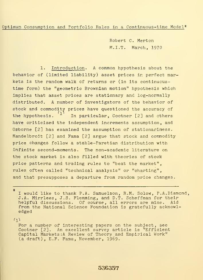
Using Ito's Lemma, we differentiate (10') to get

(11) dW «= V'^ N.dP. + y" dN.P. + 77" dN.dP^^iii ^1 11 /Ji ilThe last two terms', V^ dN.P. + V" dN.dP., are the net^ \ 11 ^1 1 1

'

value of additions to wealth from sources other than capital

gains. Hence, if dy(t) = (possibly stochastic) instan-

taneous flow of non-capital gains (wage) income, then we have

that

(12) dy - C(t)dt = 2^ ^^1^1 + YT dN^dP^

From (11) and (12), the budget or accumulation equation is

written as

(13) dW =J^^

N^(t)dP^ + dy -C(t)dt

It is advantageous to eliminate N. (t) from (13) by defining

a new variable, w.(t) = N. (t )P. (t )/W(t ) , the percentage of

wealth invested In the itll asSet at time t. Substituting

for d?^/?^ from (5), we can write (13) as

(14) dW = 'S^'^w.Wa.dt - C dt + dy + P'^w.Wa.dz.•*-<iii _*—'iiiiwhere, by definition, ^ w. =1 riO11

1

.

t

Until section seven, it will be assumed that dy = o

,

i.e. all income is derived from capital gains on assets.

If one of the n-assets is "risk-free" (by convention, the

n— asset), then a = o, the instantaneous rate of return,

a , will be called r, and (l4) is re-written as

(14') dW = ^"^ w.(a.-r)Wdt + (rW-C)dt + dy + ^ "^ W.a^dz^

^10^This result follows directly from the discrete-time argu-ment used to derive (9') where -C(t)dt Is replaced by ageneral dv(t) where dv(t) is the instantaneous flow offunds from all non-capital gains sources.

It was necessary to derive (12) by starting with thediscrete-time formulation because it is not obvious fromthe continuous version directly whether dy-C(t)dt equals2^^ dN^P^ + V^ dN^dP^ or just J^^ dN^P^.

^11^There are no other restrictions on the individual w.because borrowing and short-selling are allowed.

-9-

where m = n-1 and the w- , • ••,w are unconstrained by virtue

of the fact that the relation w = 1 - V w. will ensuren Zji i

that the identity constraint in (l4) is satisfied.

^ . Optimal portfolio and consumption rules : the

equations of optimality . The problem of choosing optimal

portfolio and consumption rules for an individual who lives

T years is formulated as follows,

(15) Max E^ [ /^ u(c(t),t)dt + b(w(T),t)J

subject to: W(o) = W ; the budget con-

straint (l4)j which in the case of a

"risk-free" asset becomes (l4'); and

where the utility function (during life),

U, is assumed to be strictly concave in

C and the "bequest" function, B, is assumed

also to be concave in W.

To derive the optimal rules, the technique of stochastic

dynamic programming is used. Define

(16) J(W,P,t) = Max E, /, U(C,s)ds + b(w(T) ,t){c,w} t L t ^ 'J

where as before, "E," is the conditional expectation operator,

conditional on W(t) = W and P^(t) = P^. Define

(17) (()(w,C;W,P,t) E U(C,t) +/[J] ,^ ^

given w^(t) = w^ , C(t) = C, ¥Ct.) = W, and P^(t) = P^. ^^

Where there is no "risk-free" asset, it is assumed noasset can be expressed as a linear combination of theother assets, implying that the nxn variance-covariancematrix of returns, Q, = [cf..] where a.. = p.. a. a., isnon-singular. In the case'^when theri'^is a"*"*^ ^ "^

"risk-free" asset, the same assumption is made about the"reduced" mxm variance-covariance matrix.

'•'^" is short for the rigorous ^ , the Dynkin operator

over the variables P and W for a given set of controlsw and C. J - '^

, Ton w nl 9 .l \-i n ,:, 3

^ = 9¥ +LI!: ^l^l^-Cj 9w-^ El "l^i 9P^

1 y,ny,n^ 2 9L + lj-|n^n

p.p.a. . ^^-1^2 ZjiZji ij 1 J 3W^ 2^^i-^i 1 J ij 3P.9P,

*s?i:? fiW"3<'ij

-10-

From the theory of stochastic dynamic programming, the

following theorem provides the method for deriving the

optimal rules, C* and w*

.

Theorem I. If the P. (t) are gen-

erated by a strong diffusion process, U

is strictly concave in C, and B is con-

cave in W, then there exists a set of

optimal rules (controls), w* and C*,

satisfying 2^ w^» = 1 and J(W,P,T) = B(W,T)

and these controls satisfy

o = 4)(C«,w*;W,P,t) > (t)(C,w;W,P,t)

for t e [o,T].

From theorem I, we have that

(18) o = Max {<j>(Cvw;W,P,t)}

{C,w}

In the usual fashion of maximization under constraint, we

define the Lagrangian, L = (}> + X[l -Y"!

"^ w.] where A is

the multiplier and find the extreme points from the first-

order conditions

(19) = L^(C*,w*) = U^(C*,t) - J^

(20) = L^^(C^w*) = - X 4. J^a^W + J^^ S? '^kJ^^J^'

^ E? -^JW^kJ^/'k=l,...,n

(2,1) = L^(C*,w») = 1 - S^^i*

3 T 9 Jwhere the notation for partial derivatives is J^ = -sttj J^ = -^r-j

TT = ^ T = i:L_ T = 9^J .J ^ 3^J^C " 9C' ^i - 3P. ' ^ij " 8P.3P. '

^"^ ^jW ~ 9P.9W

For a heuristic proof of this theorem and the derivationof the stochastic Bellman equation, see Dreyfus [4] andMerton [12]. For a rigorous proof and discussion ofweaker conditions, see Kushner [9], chapter IV especiallytheorem 7-

-11-

Because L^^^ = <^^^ = U^^^ < 0, L^^ ^*C

^ °'

^k k

L afW^J,,,,; L = 0, k ?< J, a sufficient condition^k^k - ^ WW ^v^i ' ^ '

for a unique Interior maximum Is that J,„, < (I.e. that^ WWJ be strictly concaVe In W) . That assumed, as an Immediate

consequence of differentiating (19) totally v;lth respect to

W, we have

(22) ^^ >^ ' 9W

To solve explicitly for C* and w* , we solve the n+2

non-dynamic implicit equations, (19) - (21), for C*, and

w*, and X as functions of J,,, J,nr> J^ttj W, P and t. Then' W' WW' jW' '

C* and w* are substituted in (l8) which now becomes a second-

order partial differential equation for J, subject to the

boundary condition J(W,P,T) = B(W,T) . Having (in principle

at least) solved this equation for J, we then substitute

back into (19) - (21) to derive the optimal rules as func-

tions of W, P, and t. Define the inverse function

G = CU^]~^ Then from (19),

(23) C» = G(J^,t)

To solve for the w.*, note that (20) is a linear system in

VT * and hence can be solved explicitly. Define

(24) ^ = [a..] , the nxn variance-covarlance matrix

Eliminating X from (20), the solution for w*, can be written as

(.25) w« = h^(P,t) + m(P,W,t)g^(P,t) + f^(P,W,t), k=l,...,n

wh^- E>k ~= 1' S? ^k ^ °' -^^S% ^

^16^

Q exists by the assumption on fi in footnote 12.

(continued)

-12-

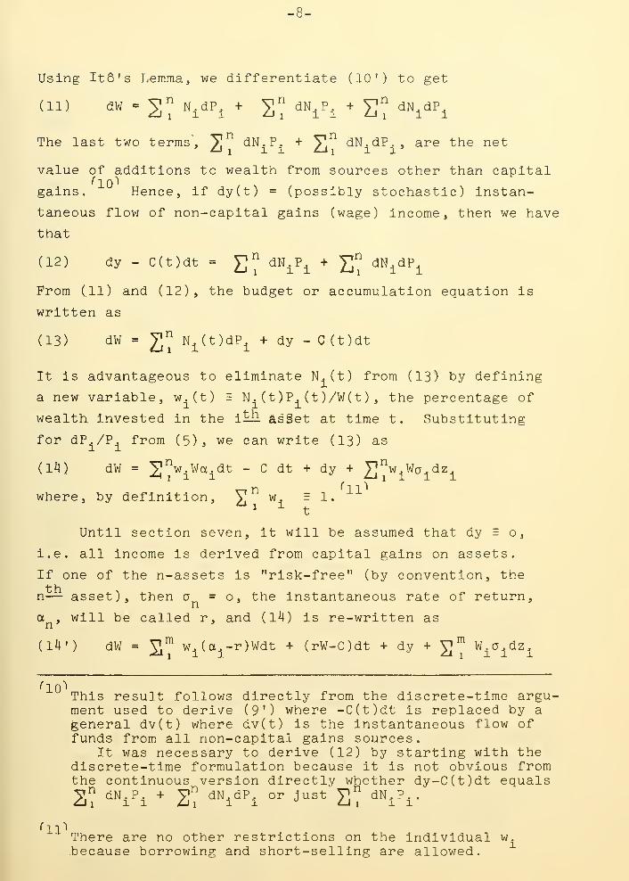
Substltutlng for w* and C* In (l8), we arrive at the

fundaftiental partial differential equation for J as a function

of W, P, and t.

(26) = UCG

+ Y^^ J,a,P. + i p'^y'^J. .a.,P.P, + F V'' J.TrP.ZJi 1 1 1 2 Liilxi ij ij 1 J r Zji jW J

W

WW[c? S>.i%V-(2?S?^i»0^]

subject to the boundary condition J(W,P,T) = B(W,T). If

(26) were solved, the solution J could be substituted into

(23) and (25) to obtain C* and w* as functions of W, P, and t.

For the case where one of the assets is "risk-free",

the equations are somewhat simplified because the problem

can be solved directly as an unconstrained maximum by. elim-

inating w as was done in (l4')-. In this case, the optimal

proportions in the risky assets areT J P

(27) w* = -j—TT V V, .(a ) - ^—Tj- , k=l,...,m.k JwwW ^1 kj J-r J,„,Wk ^ww"" " ' ^^ ^"' ^WW'

The partial differential equation for J corresponding to

(26) becomes

im

^Jw"

(.28) = U[G,T] + J^ + J^ [rW-G]+Y^^^

^±°'±'^±

+ 4 r-^ yi/" J a,,p.p, - ^r^ J,,,P,(a. s

2 £ji £>i ij IJ 1 J Jmu^i JW y j-r)

J'^ ^T, z: v,j(.,-r,(c.-., - ^Aii^s^iw^jw^ij^^jWW ' ^1 ^0 - J --yy

''16'' (continued)

-13-

subject to the boundary condition J(W,P,T) = B(W,T)

.

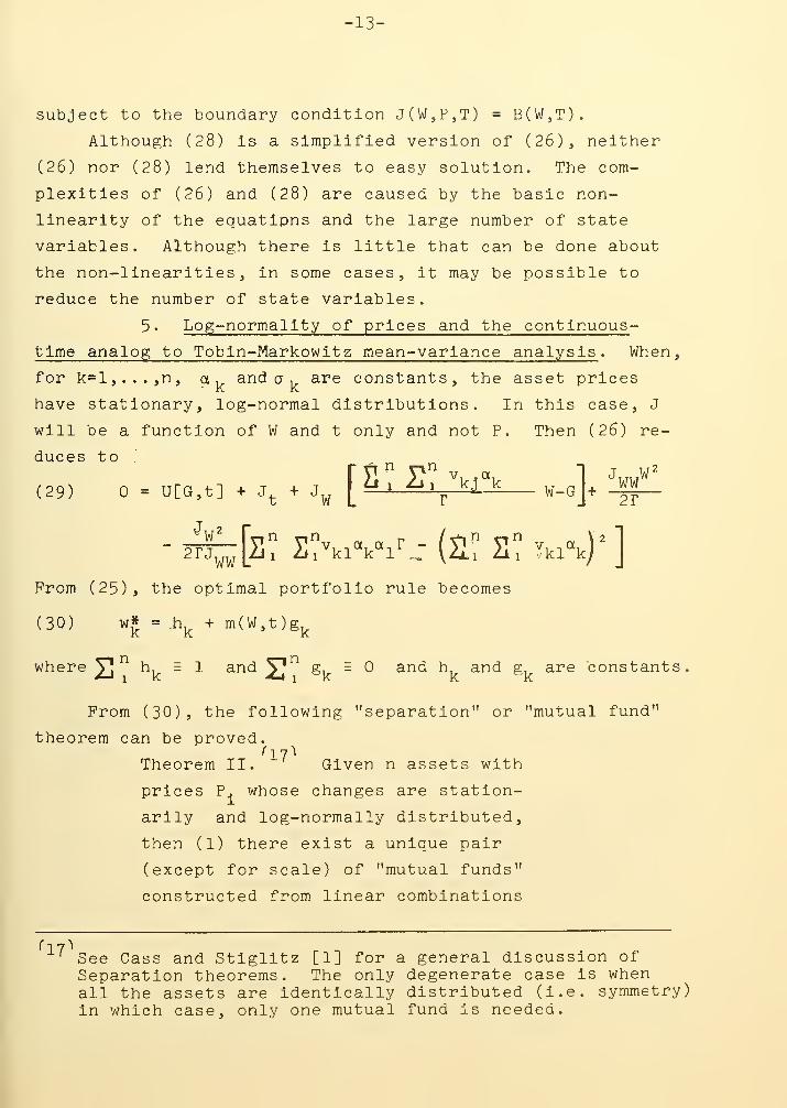
Although (28) Is a simplified version of (26), neither

(26) nor (28) lend themselves to easy solution. The com-

plexities of (26) and (28) are caused by the basic non-

llnearlty of the equatlpns and the large number of state

variables. Although there Is little that can be done about

the non-llnearlties 5 In some cases. It may be possible to

reduce the number of state variables.

5 . Log-normality of prices and the continuous -

time analog to Tobln-Markowitz mean-variance analysis . When,

for k:=l,...,n, a, and ct , are constants, the asset prices

have stationary, log-normal distributions. In this case, J

will be a function of W and t only and not P. Then (26) re-

duces tor P '^ P" V a 1

(29) = u[G,t] + Jt "^-^w I r

^^ ~^"^J"^

WW2r

^w^

WW [a? S>,cAV,:(ll" S"^H%)']From (25), the optimal portfolio rule becomes

(30) w* = h^ + m(W,t)gj^

where 2 ^v - -^ ^'^'^ 2 ^v ~ '^ ^^^ ^v ^""^ ^v ^^^ "constants.

From (30), the following "separation" or "mutual fund"

theorem can be proved.

Theorem II. Given n assets with

- prices P. whose changes are station-

arily and log-normally distributed,

then (1) there exist a unique pair

(except for scale) of "mutual funds"

constructed from linear combinations

' See Cass and Stiglltz [1] for a general discussion ofSeparation theorems. The only degenerate case is whenall the assets are identically distributed (I.e. symmetry)in which case, only one mutual fund Is needed.

-14-

of these assets such that, Independent

of preferences (i.e. the form of the

utility function) wealth distribution,

or time horizon, individuals will be

indifferent between choosing from a

linear combination of these two funds

or a linear combination of the original

n assets. (2) If P„ is the price per

share of either fund, then P„ is log-

normally distributed. Further (3) if

6, = percentage of one mutual fund's

value held in the k— asset and if

X, = percentage of the other mutual

fund's value held in the k— asset,

then one can find that

"^k" ^k

"*"

^k 'k«l,. . . ,n

and X, = h, , k=l,...,n.k k ' ' '

Proof: (1) (30) is a parametric representation of a line in

Sn * ''18''

w, =1. Hence, there exist

two linearly independent vectors (namely, the vectors of

asset proportions held by the two mutual funds) which form a

basis for all optimal portfolios chosen by the individuals.

Therefore, each individual would be indifferent between

choosing a linear combination of the mutual fund shares or a

linear combination of the original n assets.

(2) Let V = N„P„ = the total value of (either) fund

where N„ = number of shares of the fund outstanding. Let

N, = number of shares of asset k held by the fund and

u, = N, P, /V = percentage of total value invested in the

k -^ asset. Then V =2 N^P^ and

(31) dv = 2? V^k ^ S? V\ ^E ^V\= N^dP^ + P^dN^ + dP^dN^

See [1], page 15.

-15-

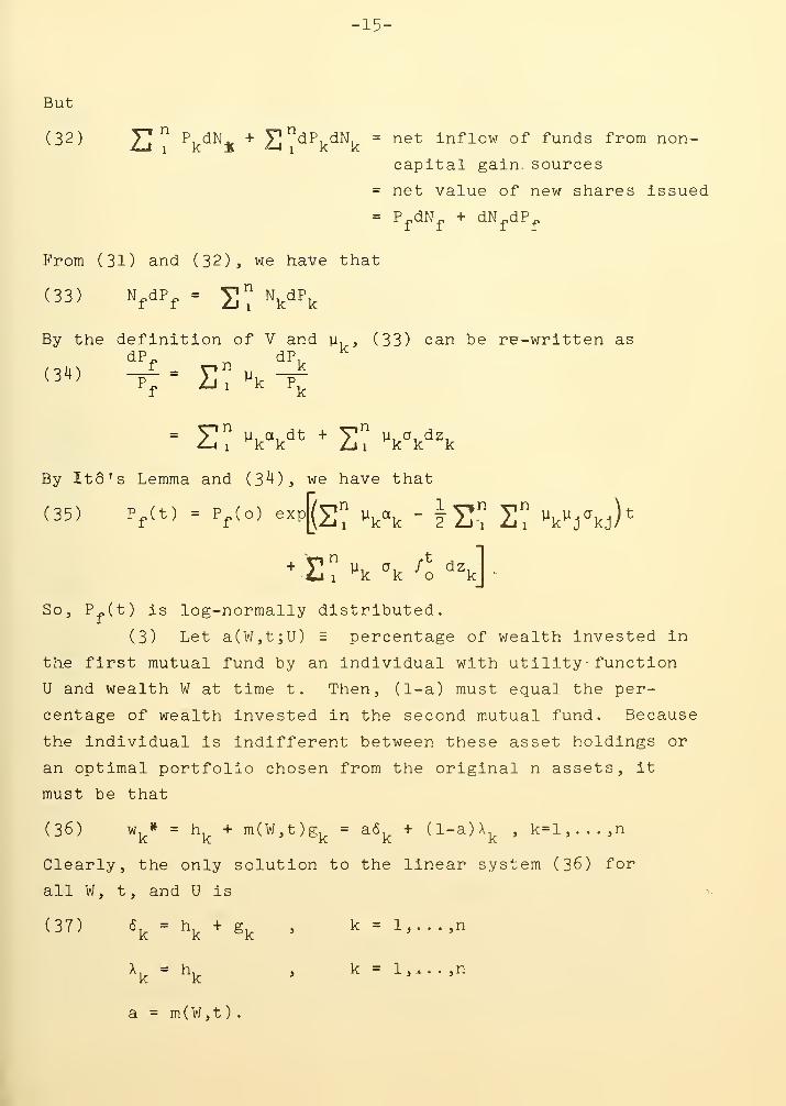
But

(32) J^^ ^k^^**" Ij'^^^k^\ "^ ^^^ inflow of funds from non-

capital gain sources

= net value of new shares issued

= P^dN^ + dN^dP^

From (31) and (32), we have that

(33) N,dP^ = 2? \^\

By the definition of V and y, , (33) can be re-written asdP„ dP,

By It8's Lemma and (3^), we have that

(35) Pj.(t) = P,(o) exp[(2^ v^a^ - ijj.";2^ Vj'lcj)'

So, P^(t) is log-normally distributed.

(3) Let a(W,t;U) = percentage of wealth invested In

the first mutual fund by an individual with utility - function

U and wealth W at time t. Then, (1-a) must equal the per-

centage of wealth invested in the second mutual fund. Because

the individual is indifferent between these asset holdings or

an optimal portfolio chosen from the original n assets, it

must be that

(36) Wj^* =^k

"^ m(W,t)g^ = aS^ + (l-a)X^ , k=l,...,n

Clearly, the only solution to the linear system (36) for

all W, t, and U is

(37) \ =^k

"^

^k 'k = 1,. . .,n

X^ = h^ , k = 1,^. . ,n

a = m(W,t)

.

-16-

Note thatY.'l \- S? ^\ -^

^k^ = ^ ^-^ S? \ = S? \ = 1'

Q.E.D.

For the case when one of the assets Is "risk-free", there

Is a corollary to theorem II. Namely,

Corollary. If one of the assets is

"risk-free", then one of the two

mutual funds will contain only this

asset. If ^].

- percentage of the

total value of the "risky" mutual

fund invested in the k— asset, then

^k =11? ^kJ^^'j-^^/S? S? ^ij^^j-^^'k=l,...,m,

Proof. By the assumption of stationary log-normal prices,

(27) reduces to

(38) w^. -'^ ^-v^jCa^-r), k=l,...,m

and

(39) w * = 1 - yV * = 1 + ^-\. V"" y"' V. .(a.-r)

By the same argument as in the proof of theorem II, (38) and

(39) define a line in the hyperplane defined by Y^ '^w . * = 1^-1

1 1

and

^k =S? ^kj^^J-^^/S? 2? ^ij^^J-^^' V°' k=l,...,m

6=0 ; A =1 k*n,n ' k

Q.E.D,

Thus, if we have an economy where all asset prices are

log-normally distributed, the investment decision can be

divided into two parts by the establishment of two financial

intermediaries (mutual funds) to hold all individual secu-

rities and to issue shares of their own for purchase by in-

dividual investors. The separation is complete because the

"instructions" given the fund managers, namely to hold pro-

-17-

portlons 6, and X, of the k— security, k=l,...,n, depend

only on the price distribution parameters and are Independent

of individual preferences, wealth distribution, or age

distribution.

The similarity of this result to that of the classical

Tobln-Markowltz analysis is clearest when one examines

closely the investment rule given to the "risky" fund's man-

ager when there exists a "risk-free" asset (money) with zero

return (r=0). It is easy to show that the 6, proportions

prescribed in the corollary are derived by finding the locus

of points in the (instantaneous) mean-standard deviation

space of composite returns which minimize variance for a

given mean, and then by finding the point where a line

drawn from the origin is tangent to the locus. This point

determines the 6, as is illustrated in figure 1.

figure 1.

Given the a*, the 6 are determined. So the log-normal

assumption in the continuous-time model is sufficient to

allow the same analysis as in the static mean-variance

model but without the objectionable assumptions of quadratic

utility or normality of the distribution of absolute price

changes. (Log-normality of price changes is much less ob-

jectionable, since this does invoke "limited liability" and

by the central limit theorem is the only regular solution to

-18-

any continuous-space. Infinitely-divisible process In time.)

An Immediate advantage for the present analysis Is that

whenever log-normality of prices Is assumed, we can work,

without loss of generality, with Just two assets, one "risk-

free" and one risky with Its price log-normally distributed.

The risky asset can always be thought of as a composite asset

with price P(t) defined by the process

(40) ^ = adt +adz

m T-im / N / ^-im v-iin

where

(41) a -as: s: ^j'^j-'v n: s: -ij(-j->

6 . Explicit solutions for a particular class of

utility functions . On th,e assumption of log-normality of

prices, some characteristics of the asset demand functions

were shown, If a further assumption about the preferences

of the individual is made, then equation (28) can be solved

in closed fonm, and the optimal consumption and portfolio

rules derived explicitly. Assume that the utility function

for the Individual, U(C,t), can be written as U(C,t) = e~'^^V(C)

where V is a member of the family of utility functions whose

measure of absolute risk aversion is positive and hyperbolic

in consumption, i^e. A(C) = -V"/V' = 1/ /j^ + n/p) > 0,

subject to the restrictions

(42) Y ^ 1; 3 > 0; (^ + n) > 0;_ n = 1 if Y= ^°° •

All members of the HARA (hyperbolic absolute risk-aversion)

family can be expressed as

(43) V(C) = ii^ (^ + n)^

-19-

This family Is rich. In the sense that by suitable adjustment

of the parameters, one can have a utility function with

absolute or relative risk aversion Increasing, decreasing,

or constant.

ri9^

table 1. Properties of KARA Utility Functions

A(C) = 1>

1-Y

(Implies n > for y > 1)

A'(C) = -1

-^'(^%tr >

< for - oo < Y < 1

for 1 < Y < '^

= for Y = ± °°

Relative risk aversion RCC) = -V"C/V' = A(C)C

R'(C) = n/gw^ > for n>0(-°°<_Yl°°jY7^1)= for n =

^ for ri<0(-«><Y<l)

Note that Included as members of the HARA family are the widely-used iso-elastlc (constant relative risk aversion), exponen-tial (constant absolute risk aversion), and quadratic utilityfunctions. As is well known for the quadratic case, the mem-bers of the HARA family with y > 1 are only defined for arestricted range of consumption, namely < C < (y -l)ri/B.

[6], [10], [5], [13], [1], and [12] discuss the propertiesof various members of the HARA family in a portfolio context.Although this is not done here, the HARA definition can begeneralized to include the cases when Yj 3, and ri are fuhe-tlohs of time subject to the restrictions in (42).

-20-

Wlthout loss of generality, assume that there are two assets,

one "risk-free" asset with return r and the other, a "risky"

asset whose price is log-normally distributed satisfying

(40). From (28), the optimality equation for J is

2 -Pt e

(41|) =^^-'^''

eL~~6~^-'

'~""^

"^t"^ [(1-Y)n/B + rWj J^

V (g-r) ^

WW

subject to J(W,T) = 0. The equations for the optimal

consumption and portfolio rules are. 1

pt

.

(45)

and

c.(., =ilfX)[l_^] ^-\ . (-da

(*6) w.(t)=J^ (5=|1)^ urw °

where w*(t) is the optimal proportion of wealth invested in

the risky asset at time t. A solution to (44) is

(47) J(W,t) = ,e-'(e-''4'^'-""' '"""^

] h ^ h (l-e-"'''-'')jYV <5 Br

where 6 = 1 - y S-^'^ v = r + (a-r)^/26a'

''20^-It is assumed for simplicity that the Individual has azerp bequest function, i.e. B H 0. If B(W,T) = H(T) (aW+b)"^,th,e basic functional form for J in (4?) will be the same.Otherwise, systematic effects of age will be involved inthe solution.

r2ilBy theorem I, there is no need to be concerned withuniqueness although, in this case, the solution is unique.

-21-

From (45), (46), and (47), the optimal consumption and

portfolio rules can be written In-, explicit form as

(48) cMt) - ^^P-^^^ '-^^^^•^ •*• ^ ^^ - e"'^^"^^)) 6n

5(1 - exp[ie^) (t-T)])^

and

(49) w*(t)W(t) = ^^W(t) + ai^(i_e^(t-T)j

The manifest characteristic of (48) and (49) Is that

the demand functions are linear in wealth. It will be shown

that the KARA family Is the only class of concave utility

functions which imply linear solutions. For notation pur-

poses, define I(X,t)c HARA(X) if "^xx^^X" l/^^tX +B) > 0,

where a and 6 are, at most, functions of time and I is a

strictly concave function of X.

Theorem III. Given the model specified

in this section, then C* = aW + b and

w*W = gW + h where a, b, g, and h are,

at most, functions of time if and only

if U(C,t) c HARA(C)

.

Proof: "If" part is proved directly by (48) and (49).

"Only if" part: Suppose w*W = gW + h and C* = aW + b

Prom (19), we have that U|^(C*,t) = J^(W,t). Differentiating

this expression totally with respect to W, we have thatdC*

U„_, -rr-r- = J,T,r or aU_,_, = J,nr End henceCC dW WW CC WW

"c " ^w•

From (46), w»W = gW + h = - J^ia-r) /J^^o^ or

-22-

So, from (50) and (51), we have that U must satisfy

-U^^/U^ = l/(a'c» + b').2

. (aa^h - ba^g)/(a-r)

(52)

where a' = <f'^g/(a-r) and b'

Hence UoHARA(C). Q.E.D.

As an immediate result of theorem III, a second theorem -

can be proved.

Theorem IV. Given the model specified

In this section, J(W,t) c HARA(W) if

and only if U c HARA(C).

Proof: "If" part is proved directly by (^7).

"C)nly If" part: suppose J(W,t) C HARA(W) . Then from (46),

w*W is a linear function of W. If (28) is differentiated

totally with respect to wealth and given the specific price

behavior assumptions of this section, we have that C* must

satisfy

v2

(53) C* = rW + ^ + ^ - w»WJ, J,

d(w*W)dW

JWWW

2J,—

-zri—

WW WW WW ' mBut if J c HARA(W), then (53) implies that C* is linear in

wealth. Hencp, by theorem III, U < HARA(C). Q.E.D.

Given (48) and (49), the stochastic process which generates

wealth when the optimal rules are applied, can be derived.

From the budget equation (l4'), we have that

(54) dW =I(w«(a-r) + r)w-C*J dt + aw*Wdz

T (a-r) ^V

"

I

I

a^6 ^_gy(t-T)Jdt +

.g-r.a6

dz X(t)

+ r ["^0] dt

where X(t) e W(t) + 6nBr

(,_,r(t-T))for < t < T and

y = (p-v)/6 . By Ito's Lemma, X(t) is the solution to

dXX \- lirT^h^"^

-23-

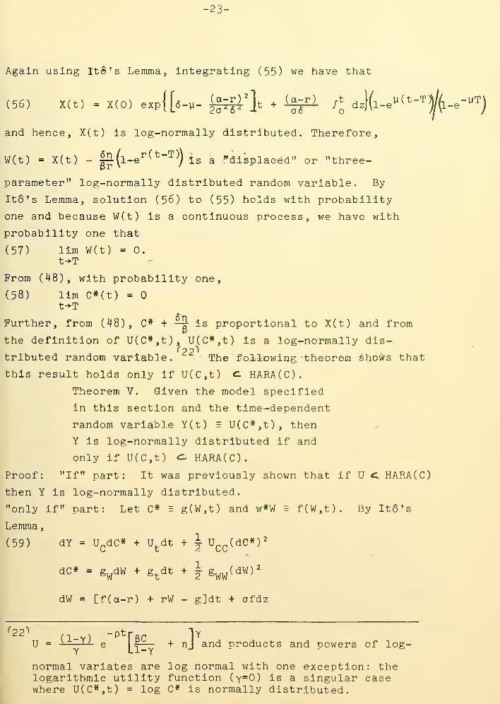
Agaln using Itc's Lemma, integrating (55) we have that

(56) X(t) = X(0) exp{[6-y- ^^^t + i^ /^ dz)(l-e^(t-T)/(l-e-^Tj

and hencBj X(t) Is log-normally distributed. Therefore,

W(t) = X(t) - |j(l-e^^^~'^'*) Is a 'displaced" or "three-

parameter" log-normally distributed random variable. By

Ito's Lemma, solution (56) to (55) holds with probability

one and because WCt) is a continuous process, we have with

probability one that

(57) lim W(t) = 0.t->T

From (48), with probability one,

(58) lim C*Ct) =

t-^-T

Further, from (48), C* + —? is proportional to X(t) and fromp

the definition of U(C*,t), U(C*,t) is a log-normally dls-

tributed random variable. ^. The following theorem shov*fs that

this result holds only if U(C,t) C HARA(C).

Theorem V. Given the model specified

in this section and the time-dependent

random variable Y(t) = U(C*,t), then

Y is log-normally distributed if and

only if U(C,t) c:^ HARA(C).

Proof: "If" part: It was previously shown that if U <1 HARA(C)

then Y is log-normally distributed.

"only if" part: Let C» e g(W,t) and w*W = f(W,t). By Ito's

Lemma,

(59) dY = U^dC* + U^dt + I U^^(de*)^

dC* = g^dW + g^dt + I gww^^^)'

dW = [f(a-r) + rW - g]dt + afdz

^22^ ,,_,, -ptr„^ lYand products and powers of log-

Y Ll-YY Ll-Y

normal varlates are log normal with one exception: thelogarithmic utility function (y=0) Is a singular casewhere U(C*,t) = log C* is normally distributed.

-24-

Because (dW)^ = a^f^dt, we have that

(60) dC* = [g„f(a-r) + g^rW-gg^ + | gww^'f'+ ^t J ^^ ^ ^%^ =

and

(61) dY =^C [sy^^^-^^ "^ ^%^ -SSw -^ I %w^'^'

-^

=t] ^ "t

CC ^Wdt + afg^U^dz

A necessary condition for Y to be log-normal is that Y satisfy

(62) ^ = F(Y)dt + bdz

where b is, at most, a function of time. If Y is log-normal,

from (6l) and (62), we have that

(63) b(t) = afg^U^/U

From the first-order conditions, f and g must satisfy

f = _ J^(a-r)/a2j^

But (63) and (64) imply that

(65)

or

hl]/o\]^ = fg^ = ^^ia-r)JJ^/o^\]^^

(66) - U^c'^^C " n(t)u^/u

where t\i.t) = (a-r)/ab(t). Integrating (66), we have that1

(67) u = [(n+i) (c+y) ?(t) ] n+i

where tit) and y are, at most, functions of time and hence

U C. ffARA ( C ) . Q . E . D

.

For the case when asset prices satisfy the "geometric"

Brownian motion hypothesis and the individual's utility

function is a member of the KARA family, the consumption-

portfolio problem is completely solved. From (48) and (49),

one could examine the effects of shifts in various parameters

on the consumption and portfolio rules by the methods of

comparative statics as was done for the Iso-elastlc case in [12]

-25-

7. Non-capital gains Income :wages . In the previous

sections. It was assumed that all Income was generated by cap-

ital gains. If a (certain) wage Income flow, dy = Y(t)dt, Is

Introduced, the optlmallty equation (18) becomes

(68) = Max [U(c,t) + / (J)]{C,w}

where the operator ^ Is defined "by jC = X + Y(t) ^tt .

This new complication causes no particular computational

difficulties. If a new control variable, C(t), and new

utility function, V(C,t) are defined by ^(t) e C(t)-Y(t) and

V(C,t) = U(C(t)+Y(t) ,t) , then (68) can be re-written as

(69) = Max [;v(C,t) +/ [J]]

{C,w}

which is the same equation as the optlmallty equation (l8)

when there is no wage Income and where consumption has been

re^r-deflned as consumption in excess of wage Income.

In partlciilar, if Y(t) e Y, a constant, and U CHARA(C),

then the optimal consumption and portfolio rules corresponding

to (48) and (49) are

iLw + r ^ + Br \ /J 6n^^°^ ^^^^ -

6 /1-exp [(p-Yv)(t-T)/6]y

and

(71) w*W =6a \ r / Bra

Comparing (70) and (71) with (48) and (49), one finds that. In

computing the optimal decision rules, the individual capi-

talizes the lifetime flow of wage Income at the market (risk-

free) rate of Interest and then treats the capitalized value

-26-

as an addition to the current stock of wealth.

The Introduction of a stochastic wage Income will cause

Increased computational difficulties although the basic

analysis Is the same as for the no-wage Income case. For a

solution to a particular example of a stochastic wage problem,

see example two of section eight.

8. Polsson processes . The previous analyses always

assumed that the underlying stochastic processes were smooth

functions of Brownlan motions and therefore, continuous In

both the time and state spaces. Although such processes are

reasonable models for price behavior of many types of liquid

assets, they are rather poor models for the description of

other types. The Polsson process is a continuous-time pro-

cess which allows discrete (or dis-continuous ) changes in

the variables. The simplest Independent Polsson process

defines the probability of an event occuring during a time

Interval of length h (where h is as small as you like) as

follows

,

(72) Prob {the event does not occur in the time interval (t,t+h)}

= ]"-- Ah + 0(h)

Prob {the event occurs once in the time interval (t,t+h)}

= Xh + 0(h)

Prob {the event occurs more than once in the time interval

(t,t+h)}= 0(h)

where 0(h) is the asymptotic order symbol defined by

(73) ^ih) is 0(h) if 11m (ij;(h)/h) '=

h^O

and X = the mean number of occurrences per unit time.

Given the Polsson process, the "event" can be defined in

a number of interesting ways. To illustrate the degree of

^^ As Hakansson [6] has pointed out, (70) and (71) are con-sistent with the Friedman Permanent Income and theModigliani Life-cycle hypotheses. However, in general,this result will not hold.

-27-

latlfeude, three examples of applications of Polsson processes

In the coneumptlon-portfollo choice problem are presented

below. Before examining these examples. It Is first necessary

to develop some of the mathematical properties of Polsson

processes. There is a theory of stochastic differential

equations for Polsson processes similar to the one for Brownian

motion discussed in section two. Let q(t) be an independent

Polsson process with probability structure as described in (72).

Let the event be that a state variable x(t) has a Jump in am-

plitude of size J where c5 is a random variable whose prob-

ability measure has compact support. Then a Polsson differ-

ential equation for x(t) can be written as

(74) dx = f(x,t)dt + g(x,t)dq

and the corresponding differential generator,^ , is defined by

(75) /^[h(x,t)]= h^ + fCx,t)h^ + E^ {XCh(x +-5g,t) - h(x,t)]}

where "E, " is the conditional expectation over the randomt

variable 5 , conditional on knowing x(t) = x, and where h(x,t)1

''24''

is a C function of x and t. Further, theorem I holds^25^

for Polsson processes.Returning to the consumption-portfolio problem, consider

first the two—asset case. Assume that one asset is a common

stock whose price is log-rnormally distributed and that the

other asset is a "risky" bond which pays an instantaneous rate

of Interest r when not in default but in the event of default,^26^

the price, of the bond becomes zero.

__For a short discussion of Polsson differential equationsand a proof of (75) as well as other references, seeKushner [9], pages 18-22.

-^ See Dreyfus [4], p. 225 and Kushner [9], chapter IV.

''26^That the price of the bond is zero in the event of defaultis an extreme assumption made only to illustrate how defaultcan be treated in the analysis. One could make the morereasonable assumption that the price In the event of defaultis a random variable. The degree of computational difficultycaused by this more reasonable assumption will depend on thechoice of distribution for the random variable as well as theutility function of the Individual.

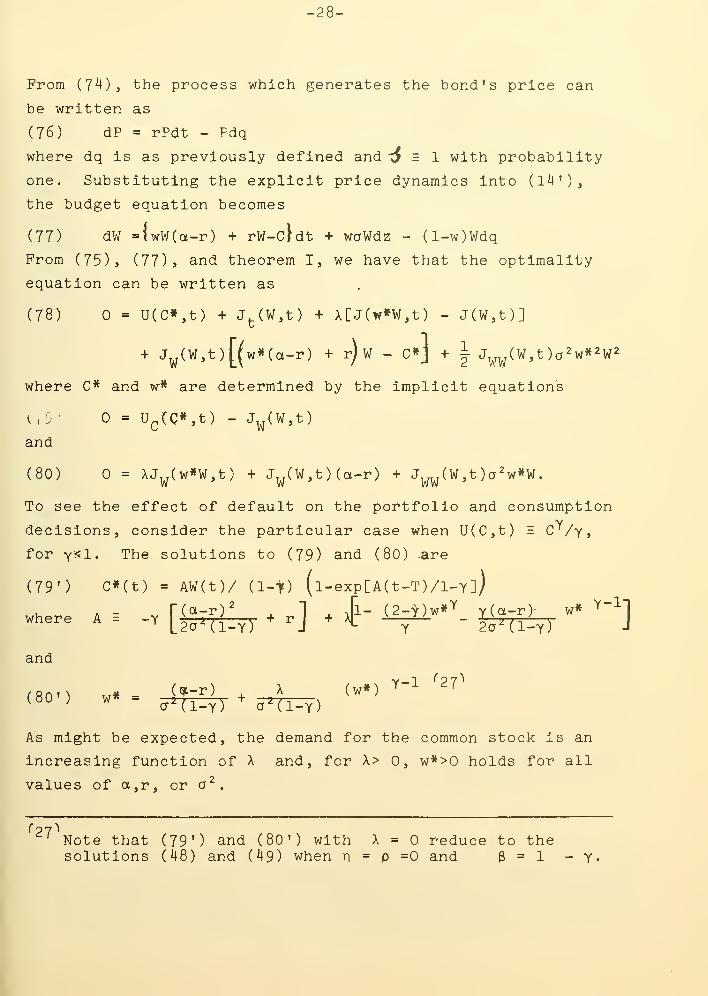
-28-

Prom (7^)5 the process which generates the bond's price can

be written as

(76) dP = rPdt - Pdq

where dq Is as previously defined and x^ = 1 with probability

one. Substituting the explicit price dynamics Into (14'),

the budget equation becomes

(77) dW ={wW(a-r) + rW-cldt + waWdz - (l-w)Wdq

From (75), (77), and theorem I, we have that the optlmality

equation can be written as

(78) = U(C»,t) + J^(W,t) + X[J(w»W,t) - J(W,t)]

+ J^(W,t)[(w*(a-r) + r)w - C»J + | J^^(\^ ,t)a^v}*^VI.

where C* and w* are determined by the implicit equation's

u9.- = U^(C*,t) - J^(W,t)

and

(80) = XJ^(w»W,t) + J^(W,t)(a-r) + Jy^(W,t )a^w*W.

To see the effect of default on the portfolio and consumption

decisions, consider the particular case when U(C,t) = C'^^/y,

for Y^l- The solutions to (79) and (80) are

C»(t) = AW(t)/ (l-t) (l-exp[A(t-T)/l-y])

^ - -^ L2a^(l-Y) + ^J + ^ -^T" " 2aHl-y) J

2

(79'')

where

and

(80' )w» - (y-r)

,X (w*) Y-1 ''27^

As might be expected, the demand for the common stock is an

Increasing function of X and, for X> 0, w*>0 holds for all

values of a,r, or a^

.

' Note that (79') and (80') with X = reduce to thesolutions (^8) and (49) when n = P =0 and 3=1 - Y-

-29-

Por the second example, consider an Individual who re-

ceives a wage, Y(t), which Is Incremented by a constant amount

e at random points In time. Suppose that the event of a wage

Increase Is distributed Polsson with parameter X. Then, the

dynamics of the wage-rate state variable are described by

(81) dY = edq, with ::^ = 1 with probability one.

Suppose further that the Individual's utility function Is of

the form U(C,t) e e~P^V(C) and that his time horizon Is in-

finite (I.e. T = <» ) . Then, for the two-asset case of sec-

tion six, the optlmallty equation can be written as

(83) = V(C») - pI(W,Y) + A[I(W,Y + £•) - I(W,Y)]

+ I^(W,Y) [(w*(a-r) + r) W + Y-C«J + | 1^^(V ,Y)a^vi*^\i^

where I(W,Y) = eP^J(W,Y,t). If It Is further assumed that_ p

V(C) = - e "/rt , then the optimal consumption and portfolio rules,

derived from (83), are

(84)

and

-(') -[«t) .^ ^ ^ (if1. „-l[p-r . if^J

(85) w«(t)w(t) = ^"7^^r ^^^

/ -1

In (84), |_W(t) + Y(t)/r + X (l-e'^^y/rw^j is the general

wealth terra, equal to the sum of present wealth and capitalized

future wage earnings. If A = 0, then (84) reduces to (70) in

^ I have shown elsewhere [[12], p. 252] that if U = e~^^V(C)and U is bounded or p sufficiently large to ensure con-vergence of the Integral and if the underlying stochasticprocesses are stationary, then the optlmallty equation (I8)can be written, independent of explicit time, as

(82) = Max [v(C) + y [I]]

^ {C,w}

where./ = ^ - P- gfand I(W,P) = e^^J(W,P,t).

A solution to (82) is called the "stationary" solution tothe consumption-portfolio problem. Because the time statevariable is eliminated, solutions to (82) are computationallyeasier to find than for the finite-horizon case.

-30-

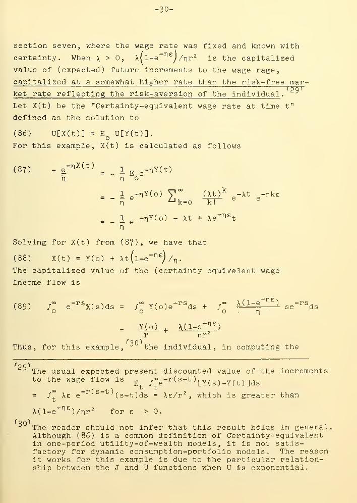
sectlon seven, where the wage rate was fixed and known with

certainty. When X > 0, xll-e~^^j/r]r^ Is the capitalized

value of (expected) future Increments to the wage rage,

capital ized at a somewhat higher rate than the risk-free mar-j_^

ket rate reflecting the risk-aversion of the Individual .

Let X(t) be the "Certainty-equivalent wage rate at time t"

defined as the solution to

(86) U[X(t)] = E^ U[Y(t)].

For this example, X(t) Is calculated as follows

(87) - e''^^^^^ = _ 1 E e"^^^^^h no

n ^ k=o k!

^ \. 1 g -nY(o) - Xt + Xe'^^^t

n

Solving for X(t) from (87), we have that

(88) X(t) = Y(o) + Xt(l-e"'^^)/TT

The capitalized value of the (certainty equivalent wage

Income flow is

rQn\ /•"> -I's^, X , ^~ v/ ^ -rs, , .<» X(l-e~^^) -rs,(o9) / e X(s)ds = / Y(o)e ds + / ^^ se ds

o o o • n

^ nol ^ i\(l-e"^^ )

r nr^

Thus, for this example, the Individual, in computing the

The usual expected present discounted value of the Incrementsto the wage flow is

^^ /"e"^^^"^

^ [Y( s )-Y(t ) ]ds

/^ Xe e"'^^^"^^ (s-t)ds = Xe/r^ , which is greater than

X(l-e~^^)/Tir2 for e > 0.

The reader should not infer that this result hdlds in general,Although (86) is a common definition of Certainty-equivalentin one-period utlllty-of-wealth models, it is not satis-factory for dynamic consumption-portfolio models. The reasonit works for this example is due to the particular relation-ship between the J and U functions when U is exponential.

-31-

present value of future earnings , determines the Certainty-

equivalent flow and then capitalizes this flow at the (cer-

tain) market rate of interest.

The third example of a Poisson process differs from the

first two because the occurrence of the event does not in-

volve an explicit change in a state variable. Consider an

individual whose age of death is a random variable. Further

assume that the event of death at each instant of time is an

independent Poisson process with parameter A. Then, the age

of death, x, is the first time that the event (of death)

occurs and is an exponentially distributed random variable

with parameter X. The optimality criterion is to

(.901 Max E^{/J

U(C,t)dt + B (w(t),t) }

and the associated optimality equation is

(91) = U(C*,t) + x[B(¥,t) - J(W,t)] +^[j] .

To derive (91), an "artificial" state variable, x(t), is con-

structed with x(t) = while the individual is alive and

x(t) = 1 in the event of death. Therefore, the stochastic

process which generates x is defined by

(92) dx = dq and 'S' = 1 with probability one

and T is now defined by x as

(93) T = mln {t|t > and x(t) = 1}.

The derived utility function, J, can be considered a function

of the state variables W, x, and t subject to the boundary

condition

OH) J(W,x,t) = B(W,t) when x = 1.

In this form, example three is shown to be of the same type

as examples one and. two in that the occurrence of the Poisson

event causes a state variable to be incremented, and (91) is

of the same form as (78) and (83).

A comparison of (91) for the particular case when B e

(no bequests) with (82) suggested the following theorem .

-^I believe that a similar theorem has been proved by

(.continued)

-32-

Theorem VI. If x is as defined in (93)

and U is such that the integral

E [/"^ U(C,t)dt] is absolutely convergent,

then the maximization of E [/"^ U(C,t)dt]

o -^0 ^ ' '

is equivalent to the maximization of

^ [/°° e~'^^U(C,t)dt] where "E " is the

conditional expectation operator over

all random variables Including t and

"^ " is the conditional expectation

operator over: all random variables

excluding x.

Proof: X is distributed exponentially and is independent of

the other random variables in the problem. Hence, we have

that

(95) E^[/J

U(C,t)dt] = /" Xe'^cJx^/J

U(C,t)at

= /"fl Xg(t)e"^'^dtdT

where g(t) e ^ [U(C,t)]. Because the integral In (95) is

absolutely convergent, the order of integration can be inter-

changed, l.e.f /"^ U(C,t)dt = /"^ f U(C,t)dt. By Inte-

gratlon by parts, (95) can be re-written as

(96) /~/;^ e"^'^g(t)dtdx = /"e"^^g(s)ds

= € /°° e '''^U(C,t)dt. Q.E.D,'O 'o

Thus, an individual who faces an exponentially-distributed

uncertain age of death acts as if he will live forever, but

with a subjective rate of time preference equal to his "force

of mortality", i.e. to the reciprocal of his life expectancy.

9. Alternative price expectations to the geometric

Brownlan motion . The assumption of the geometric Brownlan

motion hypothesis is a rich one because it is a reasonably good

''31 "^

( continued)J. A. Mlrrlees, but I have no reference. D. Cass and M.E. Yaarl

,

in "Individual Saving, Aggregate Capital Accumulation, andEfficient Growth", in Essays on the Theory of Optimal EconomicGrowth, ed. K. Shell, (M.I.T. Press 1967), prove a similartheorem on page 262.

-33-

model of observed stock price behavior and it allows the proof

of a number of strong theorems about the optimal consumption-

portfolio rules, as was illustrated in the previous sections.

However, as mentioned in the Introduction, there have been

some disagreements with the underlying assumptions required

to accept this hypothesis. The geometric Brownian motion

hypothesis best describes a stationary equilibrium economy

where expectations about future returns have settled down, and

as such, really describes a "long-run" equilibrium model for

asset prices. Therefore, to explain "short-run" consumption

and portfolio selection behavior one must Introduce alternative

models of price behavior which reflect the dynamic adjustment

of expectations.

In this section, alternative price behavior mechanisms

are postulated which attempt to capture in a simple fashion

the effects of changing expectations, and then comparisons

are made between the optimal decision rules derived under these

mechanisms with the ones derived in the previous sections.

The choices of mechanisms are not exhaustive nor are they

necessarily representative of observed asset price behavior.

Rather they have been chosen as representative examples of

price adjustment mechanisms commonly used in economic and

financial models.

Little can be said in general about the form of a solu-

tion to (28) when ct and a depend in an arbitrary manner on

the price levels. If it is specified that the utility func-

tion is a member of the KARA family, i.e.

(97) u(c,t) = -^^^ F(t) (f§^ + n)^

subject to the restrictions in (^2), then (28) can be simpli-

fied because J(¥,P,t) is separable into a product of func-

tions, one depending on W and t, and the other on P and t.

''32^This separability property was noted in [1], [5], [6],[10], [12], and [13]. It is assumed throughout this sec-tion that the bequest function satisfies the conditionsof footnote 20.

-34-

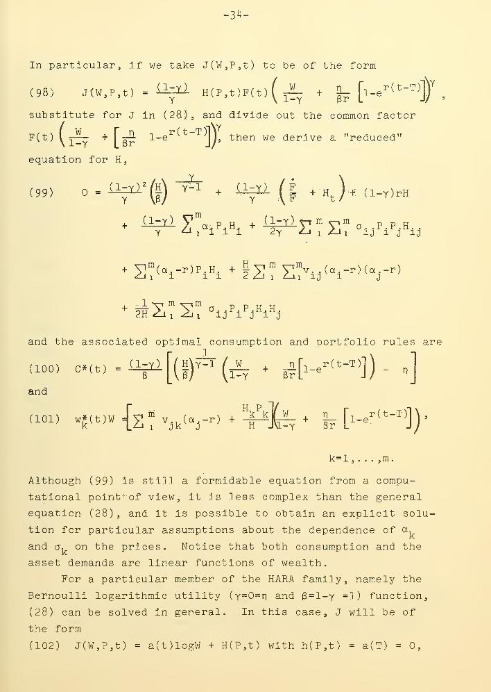
In particular. If we take J(W,P,t) to be of the form

(98) J(W,P,t) = i^:^ H(P,t)F(t)(^ . |_ [l_e-(t-T)]y

substitute for J In (28), and divide out the common factor

r(t-T)lF(t)

\1-Y L3r1-e Ij, then we derive a "reduced"

equation for H,

(99)

. (i->

X(I ^-t)+ ^-^^ [ ^- +^H, /•+ (l-Y)rH

1^X1 V\ PH. + ilzXlyrm^m ^,.p,p,H.Y '^ 1 1 1 1 2y Zj 1 2_1i ij 1 j 1,

+ yi"'(a,-r)P.H. + ly"" y"'v.,(a.-r)(a.-r)

1 x-i m -^-im

2H Zj 1 -iii 1 ij 1 J 1 J

and the associated optimal consumption and portfolio rules are_1

(100) C*(t) = -^i^p

and

(101) w*(t)W

k=l , . ..jm.

Although (99) is still a formidable equation from a compu-

tational poiht'of view, it is lees complex than the general

equation (28), and it is possible to obtain an explicit solu-

tion for particular assumptions about the dependence of a

and cr, on the prices. Notice that both consumption and the

asset demands are linear functions of wealth.

For a particular member of the KARA family, namely the

Bernoulli logarithmic utility (Y=0=ri and 6 = 1-y =1) function,

(28) can be solved in general. In this case, J will be of

the form

(102) J(W,P,t) = a(t)logW + H(P,t) with h(P,t) = a(T) = 0,

-35-

with a(t) independent of the a, and o, (and 'hence, the 'P^) •

For the case when P(t) = 1, we find a(t) = T-t and the opti-

mal rules become

(103) C» = ^T-t

and

(104) w* = 2"^ v^j(a^-r) , k=l,...,m.

For the log case, the optimal rules are identical to those

derived when a, and a, were constants, with the understanding

that the a, and a, are evaluated at current prices. Hence,

although we can solve this case for general price mechanisms,

it is not an interesting one because different assumptions

about price behavior have no effect on the decision rules.

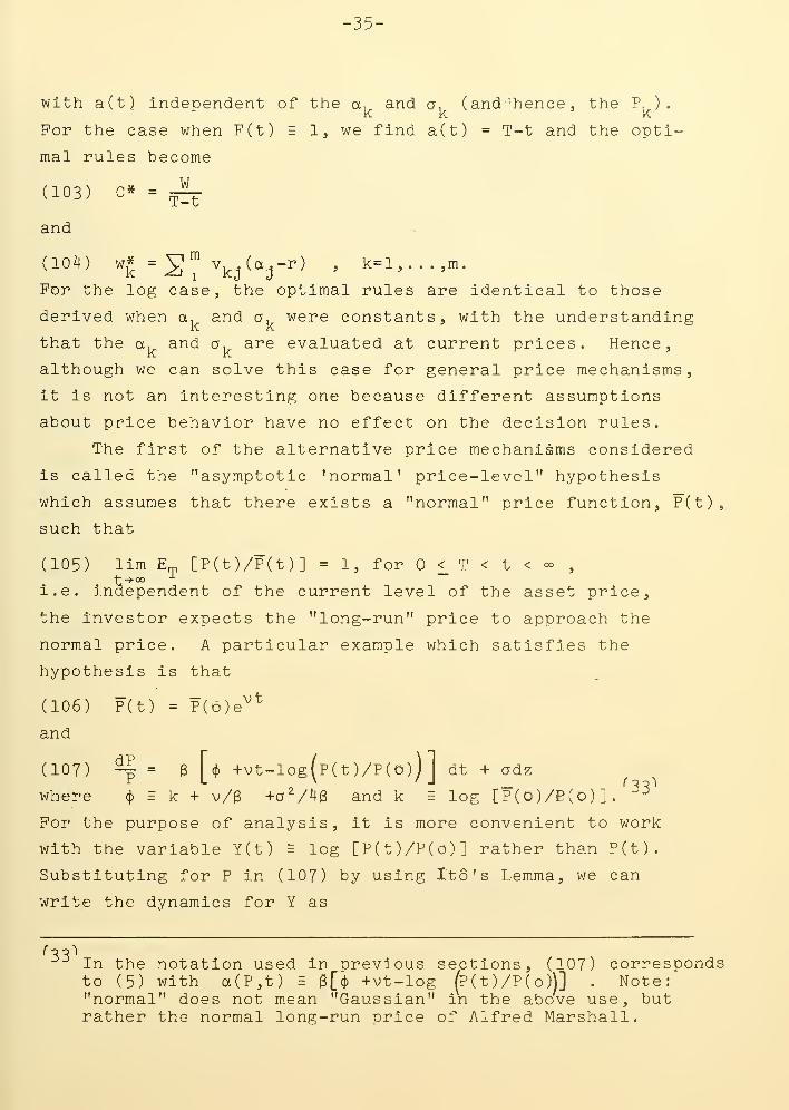
The first of the alternative price mechanisms considered

is called the "asymptotic 'normal' price-level" hypothesis

which assumes that there exists a "normal" price function, P(t),

such that

(105) lim E„ [P(t)/P(t)] = 1, for < T < t < oo,

I.e. independent of the current level of the asset price,

the investor expects the "long-run" price to approach the

normal price. A particular example which satisfies the

hypothesis is that

(106) P(t) = P(b)e^^

and

(107) ^ = 3 [(j> +vt-log(p(t)/P(0))J dt + adz

where 4) = k + v/6 +aV43 and k = log [P(o)/P(o)]. ^For the purpose of analysis, it is more convenient to work

with the variable Y(t) = log [P(t)/P(o)] rather than P(t).

Substituting for P in (107) by using Ito's Lemma, we can

write the dynamics for Y as

In the notation used in previous sections, (107) correspondsto (5) with a(P,t) = B[4) +vt-log (P(t)/P(o))] . Note:"normal" does not mean "Gaussian" in the above use, butrather the normal long-run price of Alfred Marshall.

-36-

(108) dY = &lv + vt - Y] dt + adz

where y =(fj

- a^/23. Before examining the effects of this

price mechanism on the optimal portfolio decisions, It Is

useful to Investigate the price behavior Implied by (IO6) and

(107). (107) Implies an exponentially-regressive price ad-

justment toward a normal price, adjusted for trend. By In-

spection of (108), Y is a normally-distributed random vari-

able generated by a Markov process which is not stationary

and does not have Independent Increments. Therefore, from

the definition of Y, P(t) is log-normal and Markov. Using

ItS's Lemma, one can solve (IO8) for Y(t), conditional on

knowing Y(T) , as

(109) Y(t) - Y(T) = (k + vT - ^ - Y(T)) (l-e"^^+ vt +ae"^^ /^ e^^^^

where t= t-T> 0. The instantaneous conditional variance of

Y(t) is

(110) Var [Y(t)fY(T)] =|^ (l-e'^^^).

Given the characteristics of Y(t), it is straightforward to

derive the price behavior. For example, the conditional ex-

pected price can be derived from (110) and written as

(111) E^(p(t)/P(T)) = E^ exp [Yit) - Y(T)]

= exp [(k + vT -5g - Y(T)) (l-e~^> vt

. ^(l-e-^6T)]

It is easy to verify that (105) holds by applying the appro-

priate limit process to (111). Figure 2 Illustrates the be-

havior of the conditional expectation mechanism over time.

Processes such as (IO8) are called Ornstein-Uhlenbeckprocesses and are discussed, for example, in [3]> P- 225.

-37-

,.\.YW)lY(T|.Y'j

|r(T)=?]

-<

figure 2.

For computational simplicity in deriving the optimal con-

sumption and portfolio rules, the two-asset model is used with

the individual having an infinite time horizon and a constant— Cabsolute risk-aversion utility function, U(C,t) = -e / n •

The fundamental optimality equation then is written as

(112) = -e"^-^*/n + J ^ + J^ [w* / 6(<J) + vt -Y)-r j W + rW -C*!

,1, W*^W^a^,-ro/ , , v^J_lT+ ^ J,,,, + J„g(y + vt - Y) + ^ J2 WW Y

and the associated equations for the optimal rules are

(113) w«W = -J^ [e(<}) + vt - Y) -r]/J^a^ - Jy^/J^^

and

2 -YY "^YW

(114) C» = - log (Jy)/n

Solving (112), (113), and (ll4), we write the optimal rules

in explicit form as

(115) w«W = ^ [(i + ^)(a(P,t) - r) + |4 (f^ H-v - r)]

-38-

and

(116) C» = rW + 2^1^ Y2 - ^^ (gvt + Bel) - r + b(v+ |'-r)) Y + aCt)

where a(P,t) Is the instantaneous expected rate of return de-

fined explicitly in footnote 33. To provide a basis for com-

parison, the solutions when the geometric Brownian motion hy-

pothesis IS assumed are presented as

(117) w»W = ^""F^

and

(118) C* = rW +nr

r(a-L2^

1 r(ct-r) - r

To examine the effects of the alternative "normal price" hy-

pothesis on the consumption-portfolio decisions, the (constant)

a of (117) and (ll8) is chosen equal to a(P,t) of (115) and

(ll6) so that, in both cases, the instantaneous expected return

and variance are the same at the point of time of comparison.

Comparing (115) with (117), we find that the proportion of

wealth invested in the riskv asset is always larger under the

"normal pric^e" hypothesis tj^an under the geometric Brownian motionliiypofehesis. -

' In particular* -notice 'that even if a,< r, unlike inll^e.,g<goig?t3:lc Brewnlan motion^case, g-positive amount "of the riskySSset is held.' Figures 3a" aftd "^b''. ' illustrate-'-the behavior ofthe optimal portfolio holdings.

'^^\ar. 1 {^-,.^(*-i-|i). !;.[(,-|i)(*.^.|l-.)

•v^.pr

3vt

^36 ^

For a derivation of (117) and (ll8), see [12], p. 256.

''37^ o^It is assumed that v + p- > r, i.e. the "long-run" rateof growth of the "normal " price is greater than the surerate of interest so that something of the risky asset willbe held in the short and long run.

-39-

yj*W

i^'fi) ^ilxcl"

I r P/afigure 3a,

(^W

P^>P.>^

C*<-a)

figure 3t)

.

The most striking feature of this analysis is that,

despite the ability to make continuous portfolio adjustments,

a person who believes that prices satisfy the "normal" price

hypothesis will hold more of the risky asset than one who

believes that prices satisfy the geometric Brownian motion

hypothesis, even though they both have the same utility func-

tion and the same expectations about the instantaneous mean

and variance.

The primary Interest in examining these alternative price

mechanism is to see the effects on portfolio behavior, and so,

little will be said about the effects on consumption other

than to present the optimal rule.

The second alternative price mechanism assumes the same

type of price-dynamics equation as was assumed for the geo-

metric Brownian motion: namely,

dP(119) adt + adz

-40-

However, Instead of the instantaneous expected rate of return,

a, being a constant, it is assumed that a is itself generated

by the stochastic differential equation

(120) da = B(y-a)dt + 6 (^ - ctdt)

= B(iJ-a)dt + 6adz.

The first term in (120) implies a long-run, regressive ad-

justment of the expected rate of return toward a "normal"

rate of return, y, where 3 is the speed of adjustment. The

second term in (120) implies a short-run, extrapolative ad-

justment of the expected rate of return of the "error-learn-

ing" type, where 6 is the speed of adjustment. I will call

the assumption of a price mechanism described by (119) and

(120) the "E^ Leeuw" hypothesis for Prank De Leeuw who first

introduced this type mechanism to explain interest rate be-

havior.

To examine the price behavior implied by (119) and (120),

we first derive the behavior of a, and then P. The equation

for a, (120), is of the same type as (108) described pre-

viously. Hence, a is normally distributed and is generated

by a Markov process. The solution of (120), conditional on

knowing a(T) is

(.121) a(t) - a(T) =(y- a(T)) (l-e" ^^) + 6oe~^^ /^ e^^dz,

where t = t-T> 0. Prom (121), the conditional mean and

variance of a( t ) - a(T) are

(122) E^ (a(t) - a(T)) = (y- a(T)j(l-e"^VT

and

(123) Var I a( t ) - a(T) I a([a(t) - a(T)I

a(T)]= ^F (1"^"^ ^'^

B

To derive the dynamics of P, note that, unlike a, P is

not Markov although the joint process [P,a] is. Combining

the results derived for a(t) with (119), we solve directly

-41-

for the price, conditional on knowing P(T) and a(T)

,

(124) Y(t) - Y(T)

t s-6(s-s')

+ ct6/^ /^ e ^'" " ^dz(s')ds + a /^ dz

,

t

T

where Y(t) = log [P(t!)]. From (124), the conditional mean

and variance of Y(t) - Y(T) are

(125) E^ [Y(t) - Y(T)] = (y - 1^^) T - (^-, -^^^^Xl-eg")

and

(126) Var [Y(t) - Y(T)Iy(T) = a . . 0i [b. - 2(l-e-«^)

Since P(t) is log-normal J it is straightforward to derive the

zn-Qinents for PCt) from (124), (125), and (126). Figure 4.

illustrates the behavior of the expected price mechanism.

£^rn*)|r(T)rY><<^(T)]

£^fra)|YCT)*r,/<>Ar(r)]

1

figure 4 .

The equilibrium or "long-run" (i.e. t->-°° ) distribution for!j 2^ 2

oi(t) is stationary gaussian with mean y and variance —pg— ,

and the equilibrium distribution for P(t)/P(T) is a stationary

log-normal. Hence, the long-run behavior of prices under the

De Leeuw hypothesis approaches the geometric Brownian motion.

-42-

Agaln, the two-asset model Is used with the Individual

having an Infinite time horizon and a constant absolute risk-

aversion utility function, U(0,t) = - e /ri . The

fundamental optlmality equation Is written as

-nC* r- -]

(127) = - - *"'^t

"*"

"^Ww»(a-r)W + rW - C»J

+ ^ J,n.w*2w2a2 + J 3(y-a) + ^ J fi^a"2 WW a 2 aa

+ J„ 6a^ w«WWa

Notice that the state variables of the problem are W and a,

which are both Markov, as is required for the dynamic pro-

gramming technique. The optimal portfolio rule derived from

(127) is,

J,,(a-r) J,. 6

(128) w*W = - ^ r - T^WW ^ WW

The optimal consumption rule Is the same as in (ll4). Solving

(127) and (128), the explicit solution for the portfolio rule is

(129) w»W = ;^ (,^^,,,g) [( r + « + 26 ) (a-r) - f^^^^ ]

Comparing (129) with (117) and assuming that y >r, we find

that under the De Leeuw hypothesis, the Individual will hold

a smaller amount of the risky asset than under the geometric

Brownian motion hypothesis. Note also that w*W is a decreas-

ing function of the long-run normal rate of return, y . The

interpretation of this result is that as y increases for a

given a, the probability increases that future "a's" will be

more favorable relative to the current a, and so there Is a

tendency to hold more of one's current wealth in the risk-

free asset as a "reserve" for Investment under more favorable

conditions

.

The last type of price mechanism examined differs from

the previous two in that it is assumed that prices satisfy

the geometric Brownian motion hypothesis. However, it Is also

-43-

assumed that the Investor does not know the true value of

the parameter a, but must estimate it from past data. Suppose

P is generated by equation (119) with a and a constants, and

the investor has price data back to time -t . Then, the

best estimator for a, S(t), is

(130) a(t) = ^ /^ ^where we assume, arbitrarily, that a(-T) = 0. From (130),

we have that e| S(t)j= a, and so, if we define the error

term e, = a- S(t), then (119) can be re-written as

(131) ^ = adt + adz

where dz = dz + e dt/o . Further, by differentiating (130)

we have the dynamics for S, namely

(132) dS = ^ dz/ .

Comparing (131) and (132) with (119) and (120), we see that

this "learning" model is equivalent to the special case of

the De Leeuw hypothesis of pure extrapolation (i.e. 6 = 0)

where the degree of extrapolation (6) is decreasing over time.

If the two-asset model is assumed with an investor who lives

to time T with a constant absolute risk-aversion utility

function, and if (for computational simplicity) the risk-free

asset is money (i.e. r * 0) , then the optimal portfolio rule

is

(133) w»W = -^^i^ log(|±l)a(t)

and the optimal consumption rule is

(134) c» = ^ - ^ llog (T+t) + ^ (T-t - (T+T)log(T+T)

J. f^^ M (^^ \\^ S' / (t+T) ^ Tt +t] (T-t) \1+ (t+T)iog(t+T);+ 2^^^-^-^iog|_^--tTF-jJ

By differentiating (133) with respect to t, we find that

w*W is an increasing function of time for t<t , reaches a

_il4-

raaxlmum at t = t , and then Is a decreasing function of time

for t <t <T, where t Is defined by

(135) t = [T + (l-e)T]/e. The reason for this behavior Is

that, early In life (I.e. for t<t ) , the Investor learns more

about the price equation with each observation, and hence In-

vestment In the risky asset becomes more attractive. However,

as he approaches the end of life (I.e. for t> t) , he Is gen-

erally liquidating his portfolio to consume a larger fraction

of his wealth, so that although Investment In the risky asset

Is more favorable, the absolute dollar amount Invested In the

risky asset declines.

Consider the effect on Cl33) of Increasing the number of

available previous observations (I.e. Increase x). As expect-

edj the dollar amount Invested In the risky asset Increases

monotonically . Taking the limit of (133) as t->«' , we have

that the optimal portfolio rule is

(136) w*W = '^^~2^a as T^^o

r\o

which Is the optimal rule for the geometric Brownlan motion

case when a Is known with certainty. Figure 5. Illustrates

graphically how the optimal rule changes with x .

«*v/

figure 5.

-H5-

10. Conclusion . By the introduction of Lto's

Lemma and the Fundamental Theorem of Stochastic Dynamic Pro-

gramming (Theorem I), we have shown how to systematically

construct and analyze optimal continuous-time dynamic models

under uncertainty. The basic methods employed in studying

the consumption-pDDtfolio problem are applioable to a wide-

class of economic models of decision making under uncertainty.

A major advantage of the continuous-time model over its

discrete time' analog is that one need only consider two types

of stochastic processes: functions of Brownian motions and

Poisson processes. This result limits the number of para-

meters in the problem and allows one to take full advantage

of the enormous amount of literature written about these

processes. Although I have not done so here, it is straight-

forward to show that the limits of the discrete-time model

solutions as the period spacing goes to zero are the solutions

of the continuous-time model.

A basic simplification gained by using the continuous-

time model to analyze the consumption-portfolio problem is

the Justification of the Tobin-Markowitz portfolio efficiency

conditions in the important case when asset price changes are

stationarily and log-normally distributed. With earlier

writers (Hakansson [6], Leland [10], Fischer [5], Samuelson [13]

and Cass and Stiglitz [1]), we have shown that the assumption

of the KARA utility function family simplifies the analysis

and a number of strong theorems were proved about the optimal

solutions. The introduction of stochastic wage income, risk

of default, uncertainty about life expectancy, and alternative

types of price dynamics serve to illustrate the power of the

techniques as well as to provide insight into the effects of

these complications on the optimal rules.

For a general discussion of this result, see Samuelson [l4].

-46-

References

[1] Cass, D, and Stiglltz, J.E., "The Structure of Investor

Preferences and Asset Returns, and Separability In

Portfolio Allocation: A Contribution to the Pure

Theory of Mutual Funds," Cowles Foundation Paper

[2] Cootner, P., ed.. The Random Character of Stock Market

Prices , (Cambridge: The M.I.T. Press, 1964).

[3] Cox, D.A. and Miller, H.D., The Theory of Stochastic

Processes , (New York: John Wiley and Sons, Inc.,

1968).

[4] Dreyfus, S.E., Dynamic Programming and the Calculus of

Variations , (New York: Academic Press, 1965).

[5] Fischer, S., Essays on Assets and Contingent Commodities ,

Ph.D. Dissertation, Department of Economics,

Massachusetts Institute of Technology, August, I969.

[6] Hakansson, N.H., "Optimal Investment and Consumption

Stategies Under Risk for a Class of Utility Functions,"

forthcoming in Econometrica .

[7] Ito, K., "On Stochastic Differential Equations,"

Mem. Amer. Math. Soc. No. 4 (1951),

[8] and McKean, H.P. Jr., Diffusion Processes and

Their Sample Paths , (New York: Academic Press, 1964).

[9] Kushner, H.J., Stochastic Stability and Control ,

(New York: Academic Press, 1967).

[10] Leland, H.E., Dynamic Portfolio Theory , Ph.D. Dissertation

Department of Economics, Harvard University, May, 1968.

-47-

[11] McKean, H.P. Jr., Stochastic Integrals , (New York:

Academic Press, 1969).

[12] Merton, R.C., "Lifetime Portfolio Selection Under

Uncertainty: The Continuous-time Case," Review

of Economics and Statistics , LI, (August, 1969)>

p. 2^47-257.

[13] Samuelson, P. A., "Lifetime Portfolio Selection by

Dynamic Stochastic Programming," Review of

Economics and Statistics , LI, (August, 1969)j

p. 239-246.

[14]^

, "The Fundamental Approximation

Theorem of Portfolio Analysis in Terms of Means,

Variances and Higher Moments," forthcoming in

Review of EconomiiS Studies .

[15] Stratonovich, R.L., Conditional Markov Processes and

Their Application to the Theory of Optimal Control ,

(New York: American Elsevier Publishing Co.:,1968).

Date Due

!SC15 75

JAN \ »'?

iiaEC. S I

9 1998

^^^S^

2 9 mm

Lib-26-67

3 TDfiD 003 Efi moMIT LIBRARIES

3 TOflO 03 TSfi M3

MIT LIBRARIES

3 TOflO 003 TST MMT

3 TOfio 003 TST msMIT LISRAftlES

3 TOfiO 003 7Tb OMT

ofiD 003 vTt. om