HAL Id: hal-01769324https://hal.archives-ouvertes.fr/hal-01769324v2

Submitted on 11 Oct 2018

HAL is a multi-disciplinary open accessarchive for the deposit and dissemination of sci-entific research documents, whether they are pub-lished or not. The documents may come fromteaching and research institutions in France orabroad, or from public or private research centers.

L’archive ouverte pluridisciplinaire HAL, estdestinée au dépôt et à la diffusion de documentsscientifiques de niveau recherche, publiés ou non,émanant des établissements d’enseignement et derecherche français ou étrangers, des laboratoirespublics ou privés.

Optimizing supports for additive manufacturingGrégoire Allaire, Beniamin Bogosel

To cite this version:Grégoire Allaire, Beniamin Bogosel. Optimizing supports for additive manufacturing. Structuraland Multidisciplinary Optimization, Springer Verlag (Germany), 2018, 58 (6), pp.2493-2515. hal-01769324v2

Optimizing supports for additive manufacturing

Gregoire Allaire, Beniamin Bogosel

October 11, 2018

Abstract

In additive manufacturing process support structures are often required to ensure thequality of the final built part. In this article we present mathematical models and their nu-merical implementations in an optimization loop, which allow us to design optimal supportstructures. Our models are derived with the requirement that they should be as simple aspossible, computationally cheap and yet based on a realistic physical modeling. Supportsare optimized with respect to two different physical properties. First, they must supportoverhanging regions of the structure for improving the stiffness of the supported structureduring the building process. Second, supports can help in channeling the heat flux pro-duced by the source term (typically a laser beam) and thus improving the cooling down ofthe structure during the fabrication process. Of course, more involved constraints or man-ufacturability conditions could be taken into account, most notably removal of supports.Our work is just a first step, proposing a general framework for support optimization. Ouroptimization algorithm is based on the level set method and on the computation of shapederivatives by the Hadamard method. In a first approach, only the shape and topology ofthe supports are optimized, for a given and fixed structure. In second and more elaboratedstrategy, both the supports and the structure are optimized, which amounts to a specificmultiphase optimization problem. Numerical examples are given in 2-d and 3-d.

1 Introduction

Additive manufacturing (AM) refers to the construction of objects using a layer by layer depo-sition system. Such fabrication processes have the advantage of being able to build complex orunique structures starting from a given design. Additive manufacturing offers multiple advan-tages over classical fabrication techniques, like molding or casting. In particular, the complexityof the structure is only limited by the precision given by the width of the layers, while thereare no topological constraints. Moreover, the design can be modified at any moment in thefabrication process, allowing the immediate correction of eventual design errors. Recent de-velopments in technologies regarding AM processes based on melting metal powder with theaid of a laser (or electron) beam provide great opportunities for the usage of these technologiesin various industrial branches like aeronautics, automotive, biomedical engineering, etc. [11],[23].

As already underlined in many works [16, 17, 20, 21, 26, 27, 28, 29, 30, 31, 32, 36, 38, 42, 43]a recurring issue when dealing with AM processes is the conformity of the printed structuresto the original design. Indeed, it has been observed that structures which have large portionsof surfaces which are close to being horizontal and are unsupported tend to be distorted afterthe manufacturing process. Such horizontal regions are called overhangs. These deformations,which were not in the original design, may have multiple sources. Firstly, the overhang sectionsmay be rough or deformed because the melted powder is not supported. This constraint islinked to the angle of normals to overhang surfaces with the build direction and it varies withthe material or machines involved. As a rule of thumb, it is agreed that angles greater than45 − 60 (depending on the 3D printer technology) are admissible in order to be able to build

1

the structures. Secondly, the uneven temperature distribution in the structure, which is due tothe path of the heating laser (or electron) beam, may create thermal residual stresses or thermaldilation of the structure in various directions. In order to avoid such undesired deformations,the structure can either be redesigned taking into consideration the limitation of the overhangregions and of the thermal effects, or support parts can be added with the goal of improvingthe construction process, which will be removed after the fabrication is finished.

Shape and topology optimization is by now a well known technique to automatically designstructures with optimal mechanical or thermal properties [1], [12]. Recently, there has been agrowing interest in extending these techniques in the framework of additive manufacturing.There are at least two main directions of research in this context.

First, structures can be optimized, not only for their final use, but also for their behaviorduring the building process, without requiring the addition of supports. In general, the maingoal is to limit the apparition of overhang parts during the design optimization and very oftenit is achieved by enforcing a geometric constraint on the overhang angle. In the framework ofthe SIMP method, the topology optimization of support-free structures was proposed in [33].Unfortunately, relying only on a penalization of the overhang angle is not enough. An horizon-tal overhanging part can be replaced by a zig-zag structure, which passes the angle penalizationbut is still globally an overhang. This is called the dripping effect. It shows that mechanical prop-erties should be taken into account. In the framework of the level set method, it is achieved bya combination of geometric and mechanical constraints in [4, 5]. The minimization of thermalresidual stresses or thermal deformations has been considered in [6]. The optimization of theorientation of the shape was studied in [37], [46].

Second, for given structures (optimal or not) one can optimize the placement of supports toimprove the building process and avoid any of the possible defects, previously mentioned, likeoverhang deformations or residual stresses. There are many more works in this second class ofproblems. Various ways of optimizing the supports were proposed, like sloping wall structures[27], tree-like structures [43], [21], periodic cells [42], lattices [28] and support slimming [26].A procedure for the automatic design of supports under the form of bars, with applications topolymer 3D printers was presented in [20]. An approach to optimize the topological structureof supports using the SIMP method was considered in [22]. The optimization of supports wasalso addressed in [31], where mechanical properties and geometric aspects were consider inthe optimal design process. In [14] the authors consider the optimization of supports undermechanical stresses, using the SIMP method in dimension 2. Still in the framework of theSIMP method, but adding the ease of removal as an additional constraint, the optimal designof supports was studied in [30]. The addition of supports via a level set method in orderto limit the overhang regions was studied in [16] for some two dimensional tests. A modelfor optimizing supports using compliance minimization for the linearized elasticity using theSIMP method was proposed in [34].

Of course, the two approaches can be combined in a simultaneous optimization of shapeand support. Topology optimization coupled with support structure design was considered in[36]. In [32] the simultaneous optimization of the shape, support and orientation is treated.

In the present paper we are concerned with the second approach, i.e. optimizing the sup-ports for a given structure. The main novelty of our research is to propose a general frameworkfor optimizing supports rather than just one single specific model. Inside this framework, sev-eral models are discussed for support optimization. Either one can optimize the support dis-tribution for maximizing the rigidity of the supported structure with a fixed structure, or boththe support and the structure can be optimized in a multiphase topology optimization setting.Thermal properties of the support can also be optimized in order to facilitate the evacuationof heat produced by the additive manufacturing process. A combination of both mechanicaland thermal properties can be taken into account. Following the lead of [4, 5] it is also possibleto mimick the building process and optimize supports in a layer by layer model. The common

2

point of all these models and the main characteristic of our framework is that we choose toevaluate the support performance in terms of physical models (based on partial differentialequations) rather than in terms of simple geometrical measures. To the best of our knowledge,apart from the notable exception [30], our work is the first to systematically use such a physicalmodeling of the supports in their optimization. Furthermore, we are not aware of any previouswork on support optimization based on thermal properties. Although we insist on a physicalmodeling of supports, in the mean time, having in mind to limit the computational cost, wedeliberately choose simple enough models so that support optimization is cheap and easy toimplement into automatic design softwares. Our goal is thus not to model very accurately thebuilding process and the behavior of supports but rather to obtain a global and approximateperformance of the supports which is easily taken into account in an optimization algorithm.In particular, if supports are finely spaced and form a very heterogeneous structure, our modelconsider them as an equivalent homogenized material which avoids a precise description andmeshing of all geometrical details. Of course, our models, objective functions and resulting op-timized supports should be assessed by comparison with experimental results. In this respect,a crucial issue is the removal of supports after printing. This may be a very intricate process,especially for complex 3-d shapes. One possibility is to add geometric constraints (in the spiritof [8], [9]) ensuring that any contact zone between supports and the actual shape is accessiblefrom the outside along a straight tubular hole, allowing for the passage of some tool able to cutthe supports. This is the topic of future work which is clearly out of the scope of the presentpaper. In particular, it may well be that new objective functions or models arise, based on ex-perimental evidence (for example to take into account thermal residual stresses as in [6]). Oneadvantage of our approach is that such new ingredients can easily be cast in our framework.Nevertheless, we make comparison of our optimized supports with the one obtained in [30]and those obtained by classical geometric criteria.

The content of our paper is the following. In Section 2 we focus on minimizing the me-chanical effects of overhangs, without taking into account a thermal model. In Subsection 2.1the shape is assumed to be fixed and only the supports are optimized by using a mechanicalcriterion. More precisely we minimize a weighted sum of the support volume and of the com-pliance for the union of the shape and its support, submitted to gravity. Of course, under sucha load, overhang regions of the shape will have a tendency to get supported during the opti-mization process. In Subsection 2.2 we extend our analysis to the simultaneous optimization ofthe shape and support. It involves two state equations: one for the final use of the shape (with-out supports) and another one for gravity effects during the building process. It is therefore amulti-phase optimization problem and we rely on the method proposed in [3]. Subsection 2.3makes a comparison with the more involved layer by layer model, introduced in [4, 5], restrictedhere to the case of a fixed shape.

Section 3 turns to the support optimization in order to facilitate the evacuation of the heatcoming from the laser or electron beam. In this case the model is the stationary heat equationor its long time behavior, given by the first eigenmode, posed in the union of the shape and itssupport. Thermal compliance is minimized for a given source term supported only in the shapesince thermal deformations of the support are not important. As is well known, minimizingthermal compliance can be interpreted as maximizing heat evacuation.

As explained in Section 4 our main numerical tool is the level set method [41]. Shape deriva-tives, computed by Hadamard method, are the velocities in the transport Hamilton-Jacobiequation [10]. Our optimization algorithm is a simple Augmented Lagrangian method [13].Dealing with the level set method needs certain specific tools regarding the reinitialization andthe advection of the level set function. We rely on the publicly available tools MshDist [19] andAdvect [15] from the ICSD Toolbox available online: https://github.com/ISCDtoolbox.Our partial differential equations models are solved by finite elements in the FreeFem++ soft-ware [24] which is well suited for multiphysics simulation (and is a publicly available tool too).

3

Eventually Section 5 contains our numerical test cases. At first a few examples concerningsupports which maximize the rigidity of the structure under gravity loads are presented, usingthe ideas of Section 2. Numerical examples in dimensions two and three show that our algo-rithm can handle complex cases. Then, some simulations concerning the optimization of thesupports with respect to their thermal properties are displayed in the framework of Section 3.Of course, it is possible to optimize the supports for both thermal and elastic loads, as in Section5.3. The simultaneous optimization of the shape and its support, as discussed in Section 2.2, isalso illustrated. The behavior of the support with respect to the orientation of the shape is alsoconsidered in Section 5.5. Finally, for the sake of comparison, the layer by layer algorithm, pre-sented in Section 2.3, is tested for two and three dimensional test cases. The resulting optimalsupports are not very different from the ones obtained with the simpler algorithm of Section2, showing the interest of the present approach, which is much cheaper in terms of CPU time.Comparisons with other methods for generating supports, like the model considered in [30] orthe simple geometrical criterion adding vertical supports under overhanging regions, can befound in Section 5.1.

Concluding remarks and perspectives are given in Section 6. As already said, our approachhas to be validated by experiments which will possibly indicate other possible objective func-tions and models which may be useful for support optimization. Other constraints or objectiveson supports include mitigation of thermal deformations, ease of removal, a precise geometricdescription of the supports not based on equivalent homogenized properties: they are nottreated here and will be addressed in future works. The main point of our work, as well as nayoptimization approach, is to progressively replace the expert intuition and knowledge by anautomatic process of support design, based on a physical, albeit simplified, modeling.

2 Shape optimization for minimizing the mechanical effects of over-hangs

2.1 Optimizing the Support when the Shape is Fixed

Let us consider a shape ω, which has to be printed, together with its supports S. Both S andω are open sets of Rd (with d = 2 or 3 in practice) and are not necessarily made of the samematerial. In a first stage the shape ω will be fixed and only the support S will be the opti-mized. In a second stage (see the next subsection), both the support S and the shape ω willbe optimized. Our numerical framework could be used for arbitrary build directions. In ourcomputations, however, we always suppose that the build direction is the vertical one: a struc-ture is built from bottom towards its top. A point in Rd is denoted by x = (x1, ..., xd) and thevertical direction is ed = (0, ..., 0, 1). The supported structure is denoted by Ω = S ∪ ω and isassumed to be contained in a given computational domain D, which can be interpreted as thebuild chamber. For simplicity, the build chamber will always be a rectangular box. The buildchamber D always contains the baseplate as its bottom boundary, denoted by ΓD. By defini-tion, the bottom boundary ΓD corresponds to xd = 0. We assume that the support S is clampedon the boundary ΓD of the computation domain D. The other regions of the boundary of thesupported structure Ω are traction-free, denoted by ΓN . In the following for an open domainΩ ⊂ Rd and a (d− 1)-dimensional set Γ we consider the space

H1Γ(Ω)d = u ∈ H1(Ω)d : u = 0 on Γ (1)

The deformation of the supported structure Ω is governed by the equations of linearizedelasticity. Following [5] only gravity forces are applied to Ω. Then, optimizing the support Sfor minimizing the compliance of Ω will induce minimal overhang regions. The elastic dis-placement uspt of the supported structure Ω = ω∪S is the unique solution in the space H1

ΓD(Ω)

4

(defined in (1)) to the mechanical system−div(Ae(uspt)) = ρg in Ω,

uspt = 0 on ΓD,Ae(uspt)n = 0 on ΓN .

(2)

In (2), e(u) = 12(∇u+∇uT ) is the linearized strain tensor associated to the displacement u, g is

the (vertical) gravity vector and n denotes the unit normal vector to Ω. We denote by ρ(x) thedensity of the structure Ω and by A(x) its Hooke’s tensor, which may both vary with respectto the position x. Typically, these material properties may be different in the shape ω and inthe support S, which happens often in practice. Indeed, supports are often not bulk piecesof metal but rather are some kind of lattice-thin-wall structures. However, for optimizationpurposes it is out of the question to model all these fine details and rather it is replaced here bya homogeneous effective material (or equivalent homogenized material) with different materialproperties from those of the shape. More precisely we have Ae(u) = 2µe(u) + λ div u Id, whereId is the identity matrix and µ, λ are the Young modulus and Poisson ratio, respectively. Ifµω, λω, ρω are the mechanical parameters for the shape ω and µS , λS , ρS are the correspondingparameters for the support, then

µ = µωχω + µSχS , λ = λωχω + λSχS , ρ = ρωχω + ρSχS .

We evaluate the mechanical performance of the supported structure Ω in terms of its struc-tural compliance

J(S) =

∫ω∪S

Ae(uspt) · e(uspt) dx =

∫ω∪S

ρg · uspt dx . (3)

Other objective functions would be possible. This objective function is minimized in the set Uadof admissible supports defined by

Uad = S ⊂ (D \ ω) such that ,ΓD ∩ ∂S 6= ∅, ∂ω ∩ ∂S 6= ∅.

If we do not impose any constraints then the optimization procedure will not produce relevantsupported structures since the support S will simply fill the space under the shape ω in D. Inorder to prevent this we add a constraint on the volume of the support S. This is of courserelevant from a physical point of view, since we wish to obtain optimal structures which do notuse too much material.

The constraint can be incorporated in the functional by using a Lagrange multiplier `.Therefore we will consider problems of the form

minS∈Uad

J(S) + `Vol(S), (4)

where ` is either a given penalization parameter, or a parameter which changes during theoptimization process in order to reach the equality in the volume constraint at the end of theoptimization process. When we wish to work with a volume constraint an Augmented La-grangian method is used, as described in Section 4.

In order to find numerical solutions to problem (4) we use algorithms which are basedon the derivatives of the compliance J(S) and the volume Vol(S). In the shape optimizationcontext these shape derivatives are computed by the Hadamard method [1], [40]. Given avector field θ ∈W 1,∞(Rd,Rd) we consider variations of the set S induced by θ of the form

θ 7→ Sθ = (Id + θ)(S).

5

Definition 2.1. A function F (S) of the domain is shape differentiable at S if the underlying mapθ 7→ F (Sθ) from W 1,∞(Rd,Rd) into R, defined above, is Frechet differentiable at 0. The correspondingderivative is denoted by F ′(S) and the following asymptotic expansion holds in a neighborhood of 0:

F (Sθ) = F (S) + F ′(S)(θ) + o(θ), where|o(θ)|

‖θ‖W 1,∞(Rd,Rd)

θ→0−→ 0.

Computing the shape derivative of the compliance is a classical result (see e.g. [10]). Recallthat the shape ω is fixed and only the support S may vary. Note also that, from a mechan-ical point of view, the support S always lies outside the shape ω and cannot move inside ω.Therefore, for most results in the following we make the following assumption.

Assumption 2.2. The interface ∂S ∩ ∂ω is assumed to be fixed. Therefore, all vector fields θ in theshape derivatives are assumed to satisfy θ · n = 0 on ∂S ∩ ∂ω.

Proposition 2.3. Under Assumption 2.2, the shape derivative of the compliance (3) is given by

J ′(S)(θ) =

∫∂S∩ωc

(−Ae(uspt) · e(uspt) + 2ρg · uspt

)θ · n ds

where uspt is the solution of (2) and ωc = D \ ω and ∂S ∩ ωc = ∂S \ ∂ω.

This follows at once from [10, Theorem 7]. The shape derivative is carried merely by ∂S∩ωcbecause the normal components of the vector fields θ vanish on the interface ∂S∩∂ω. This resultis a particular case of the more general result, Proposition 2.5, proved in the following section.

Eventually, it is well known that the shape derivative of the volume is given by

Vol′(S)(θ) =

∫∂S∩ωc

θ · nds.

2.2 Simultaneous Optimization of the Support and the Shape

In a second stage we consider the simultaneous optimization of the shape and the support.While in the previous subsection the support S was optimized only for counter-balancing thegravity effects during the building process, now the shape ω has also to be optimized for its finaluse, independently of the support S. Therefore, in addition to the state equation (2), accountingfor gravity effects on the supported structure S ∪ ω, we now add another state equation for ωonly, which takes into account its final use with new loads and boundary conditions. Figure 1displays the different type of boundary conditions for these two state equations on an examplewhich will be studied later in Section 5. From now on the elastic displacement, solution ofthe first state equation for the supported structure during its building process, is denoted uspt,while the other elastic displacement, solution of the second state equation for the shape duringits final use, is denoted ufin.

For its final use, the shape ω is clamped on a boundary ΓD and is loaded on another bound-ary Γ0 by some surface loads by ffin. The rest of the boundary denoted ΓN is traction-free. Themechanical properties of ω with respect to the final functionality of the shape is described bythe following second state equation

−div(Ae(ufin)) = 0 in ω,ufin = 0 on ΓD,

Ae(ufin)n = ffin on Γ0,

Ae(ufin)n = 0 on ΓN .

(5)

As already said, the boundary conditions and loadings are not the same for the two state equa-tions (2) and (5) (see Figure 1).

6

Figure 1: Different boundary conditions for the final use of the shape (left) and for the sup-ported structure (right)

The objective function to be optimized is now the sum of the compliance for (5) and that for(2)

J2(ω, S) =

∫ω∪S

ρg · uspt dx+

∫Γ0

ffin · ufin ds. (6)

Of course, more general objective functions for (5) could be studied, at the expense of introduc-ing an adjoint equation. This new objective function is minimized in the set Uad of combinedadmissible shapes and supports defined by

Uad =

(ω, S) ⊂ D such that ω ∩ S = ∅,ΓD ∩ ∂S 6= ∅, ΓD ∩ ∂ω 6= ∅, ∂ω ∩ ∂S 6= ∅.

Adding volume constraints on both S and ω, we consider the following optimization problem

min(ω,S)∈Uad

J2(ω, S) + `S Vol(S) + `ω Vol(ω), (7)

where `S , `ω are two Lagrange multipliers for the volume constraints on S and ω, respectively.Contrary to the previous section, the interface between the support S and the shape ω can nowbe optimized. Therefore, the vector fields θ in the shape derivatives do not necessarily vanishon the interface ∂S ∩ ∂ω. In other words, problem (7) is a two-phase optimization problembecause the material properties are usually not the same in the support and in the shape.

It is well known (see e.g. [3]) that computing shape derivatives for an interface betweentwo phases is a delicate issue and that the resulting formulas are complicated to use in numer-ical optimization. Typically, because of different mechanical properties A and ρ between ω andS, there will be jumps of discontinuous quantities on the interface in the shape derivative for-mula. However, as already underlined in [3, Section 2.2], shape derivatives are much simplerif we suppose that the equations (2) and (5) are solved for uspt, ufin in some finite dimensionalsubspaces. Therefore, in the following we make the following simplifying assumption, whichremains valid in our numerical computations based on finite element methods.

Assumption 2.4. Let Vh andWh be finite dimensional subspaces ofH1ΓD

(ω)d andH1ΓD

(Ω)d (see (1) fortheir definition), respectively. Let uhfin be the solution of the approximate variational formulation of (5)in Vh and uhspt be the solution of the approximate variational formulation of (2) in Wh. In the followingwe work with these discrete solutions, and for the simplicity of notation, we drop the discrete index h.

We now give the shape derivative of J2(ω, S) when both the shape and the support aredeformed by a vector field θ.

Proposition 2.5. Under Assumption 2.4, for any vector field θ ∈ W 1,∞(Rd,Rd), the shape derivativeof J2(ω, S), defined by (6), is given by

J ′2(ω, S)(θ) =

∫∂ω\∂S

j1θ · n ds+

∫∂ω∩∂S

j2θ · n ds+

∫∂S\∂ω

j3θ · n ds,

7

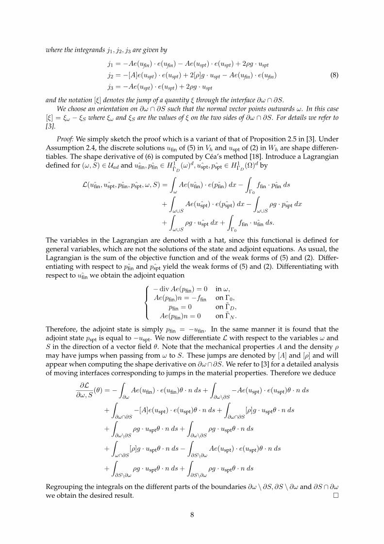
where the integrands j1, j2, j3 are given by

j1 = −Ae(ufin) · e(ufin)−Ae(uspt) · e(uspt) + 2ρg · uspt

j2 = −[A]e(uspt) · e(uspt) + 2[ρ]g · uspt −Ae(ufin) · e(ufin) (8)

j3 = −Ae(uspt) · e(uspt) + 2ρg · uspt

and the notation [ξ] denotes the jump of a quantity ξ through the interface ∂ω ∩ ∂S.We choose an orientation on ∂ω ∩ ∂S such that the normal vector points outwards ω. In this case

[ξ] = ξω − ξS where ξω and ξS are the values of ξ on the two sides of ∂ω ∩ ∂S. For details we refer to[3].

Proof: We simply sketch the proof which is a variant of that of Proposition 2.5 in [3]. UnderAssumption 2.4, the discrete solutions ufin of (5) in Vh and uspt of (2) in Wh are shape differen-tiables. The shape derivative of (6) is computed by Cea’s method [18]. Introduce a Lagrangiandefined for (ω, S) ∈ Uad and ˆufin, ˆpfin ∈ H1

ΓD(ω)d, ˆuspt, ˆpspt ∈ H1

ΓD(Ω)d by

L( ˆufin, ˆuspt, ˆpfin, ˆpspt, ω, S) =

∫ωAe( ˆufin) · e( ˆpfin) dx−

∫Γ0

ffin · ˆpfin ds

+

∫ω∪S

Ae( ˆuspt) · e( ˆpspt) dx−∫ω∪S

ρg · ˆpspt dx

+

∫ω∪S

ρg · ˆuspt dx+

∫Γ0

ffin · ˆufin ds.

The variables in the Lagrangian are denoted with a hat, since this functional is defined forgeneral variables, which are not the solutions of the state and adjoint equations. As usual, theLagrangian is the sum of the objective function and of the weak forms of (5) and (2). Differ-entiating with respect to ˆpfin and ˆpspt yield the weak forms of (5) and (2). Differentiating withrespect to ˆufin we obtain the adjoint equation

−divAe(pfin) = 0 in ω,Ae(pfin)n = −ffin on Γ0,

pfin = 0 on ΓD,

Ae(pfin)n = 0 on ΓN .

Therefore, the adjoint state is simply pfin = −ufin. In the same manner it is found that theadjoint state pspt is equal to −uspt. We now differentiate L with respect to the variables ω andS in the direction of a vector field θ. Note that the mechanical properties A and the density ρmay have jumps when passing from ω to S. These jumps are denoted by [A] and [ρ] and willappear when computing the shape derivative on ∂ω∩∂S. We refer to [3] for a detailed analysisof moving interfaces corresponding to jumps in the material properties. Therefore we deduce

∂L∂ω, S

(θ) = −∫∂ωAe(ufin) · e(ufin)θ · n ds+

∫∂ω\∂S

−Ae(uspt) · e(uspt)θ · n ds

+

∫∂ω∩∂S

−[A]e(uspt) · e(uspt)θ · n ds+

∫∂ω∩∂S

[ρ]g · usptθ · n ds

+

∫∂ω\∂S

ρg · usptθ · n ds+

∫∂ω\∂S

ρg · usptθ · n ds

+

∫ω∩∂S

[ρ]g · usptθ · n ds−∫∂S\∂ω

Ae(uspt) · e(uspt)θ · n ds

+

∫∂S\∂ω

ρg · usptθ · n ds+

∫∂S\∂ω

ρg · usptθ · n ds

Regrouping the integrals on the different parts of the boundaries ∂ω \ ∂S, ∂S \ ∂ω and ∂S ∩ ∂ωwe obtain the desired result.

8

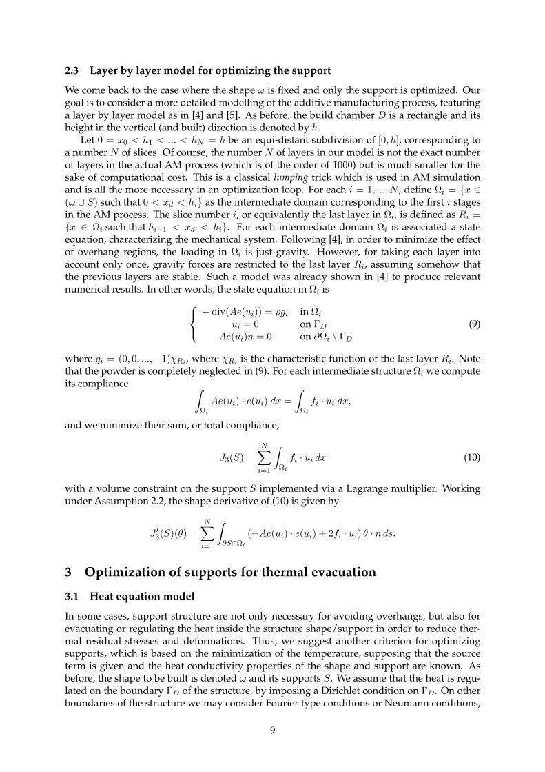
2.3 Layer by layer model for optimizing the support

We come back to the case where the shape ω is fixed and only the support is optimized. Ourgoal is to consider a more detailed modelling of the additive manufacturing process, featuringa layer by layer model as in [4] and [5]. As before, the build chamber D is a rectangle and itsheight in the vertical (and built) direction is denoted by h.

Let 0 = x0 < h1 < ... < hN = h be an equi-distant subdivision of [0, h], corresponding toa number N of slices. Of course, the number N of layers in our model is not the exact numberof layers in the actual AM process (which is of the order of 1000) but is much smaller for thesake of computational cost. This is a classical lumping trick which is used in AM simulationand is all the more necessary in an optimization loop. For each i = 1, ..., N , define Ωi = x ∈(ω ∪ S) such that 0 < xd < hi as the intermediate domain corresponding to the first i stagesin the AM process. The slice number i, or equivalently the last layer in Ωi, is defined as Ri =x ∈ Ωi such that hi−1 < xd < hi. For each intermediate domain Ωi is associated a stateequation, characterizing the mechanical system. Following [4], in order to minimize the effectof overhang regions, the loading in Ωi is just gravity. However, for taking each layer intoaccount only once, gravity forces are restricted to the last layer Ri, assuming somehow thatthe previous layers are stable. Such a model was already shown in [4] to produce relevantnumerical results. In other words, the state equation in Ωi is

−div(Ae(ui)) = ρgi in Ωi

ui = 0 on ΓDAe(ui)n = 0 on ∂Ωi \ ΓD

(9)

where gi = (0, 0, ...,−1)χRi , where χRi is the characteristic function of the last layer Ri. Notethat the powder is completely neglected in (9). For each intermediate structure Ωi we computeits compliance ∫

Ωi

Ae(ui) · e(ui) dx =

∫Ωi

fi · ui dx,

and we minimize their sum, or total compliance,

J3(S) =

N∑i=1

∫Ωi

fi · ui dx (10)

with a volume constraint on the support S implemented via a Lagrange multiplier. Workingunder Assumption 2.2, the shape derivative of (10) is given by

J ′3(S)(θ) =N∑i=1

∫∂S∩Ωi

(−Ae(ui) · e(ui) + 2fi · ui) θ · nds.

3 Optimization of supports for thermal evacuation

3.1 Heat equation model

In some cases, support structure are not only necessary for avoiding overhangs, but also forevacuating or regulating the heat inside the structure shape/support in order to reduce ther-mal residual stresses and deformations. Thus, we suggest another criterion for optimizingsupports, which is based on the minimization of the temperature, supposing that the sourceterm is given and the heat conductivity properties of the shape and support are known. Asbefore, the shape to be built is denoted ω and its supports S. We assume that the heat is regu-lated on the boundary ΓD of the structure, by imposing a Dirichlet condition on ΓD. On otherboundaries of the structure we may consider Fourier type conditions or Neumann conditions,

9

since the conductivity of the powder is significantly smaller than the conductivity of the fusedstructure.

In the following, we denote by k = kωχω + kSχS the conductivity throughout the structure.Here kω is the constant conductivity in the shape ω and kS that in the support S. These twovalues kω and kS may be different since the support can be an equivalent homogenized mate-rial, with distinct properties from the bulk material occupying the shape. The source term f isassumed to be supported inside the shape ω. Fourier boundary conditions may be considered,in view of the fact that the heat may dissipate in the powder region or by radiation in the up-per layer. However, since it is considered that the main source of heat evacuation is throughthe baseplate, we simplify our model by considering homogeneous Neumann boundary con-ditions. Thus, the thermal model reads

−div(k∇T ) = fχω in S ∪ ωk(x)∇T · n = 0 on ΓN

T = 0 on ΓD

(11)

The shape ω is assumed to be fixed and thermal compliance is minimized for all admissiblesupports

minS∈Uad

F(S) =

∫ωfTdx. (12)

The volume constraint is added using a Lagrange multiplier.

Proposition 3.1. Under Assumption 2.2 the shape derivative of the thermal compliance (12) related tothe system (11) is given by

F ′(S)(θ) = −∫∂S\∂ω

k|∇T |2θ · nds. (13)

Proof: This is a classical result and we briefly sketch the main idea of the proof. Considerthe Lagrangian defined for S ∈ Uad and T , p ∈ H1

ΓD(D) by

L(T , p, S) =

∫S∪ω

k∇T · ∇p dx−∫ωfp dx+

∫ωfT dx

obtained by summing the variational form of (11) with the functional F(S). The partial deriva-tive of L with respect to p gives the state equation and the partial derivative with respect to Tyields the adjoint equation. This is a self-adjoint case and the adjoint is simply p = −T . Thepartial derivative of Lwith respect to S gives the shape derivative of F given in (13).

3.2 Spectral model

In truth, heat evacuation is a transient phenomenon, which is governed by the heat equationρ∂u

∂t− div(k∇u) = 0 in S ∪ ω

u(t = 0) = u0 in S ∪ ωu = 0 on ΓD

k∇u · n = 0 on ΓN ,

where ρ = ρωχω + ρSχS is the product of density by specific heat and k = kωχω + kSχS isthe conductivity. Since the heat operator is self-adjoint with compact resolvent, its spectrumconsists of an increasing sequence of eigenvalues. Furthermore, the associated eigenfunctionsform a Hilbert basis for the space H1

ΓD(Ω). In the following λk and wk denote the eigenvalues

10

and eigenvectors of the heat operator. It is well known (see, for example [2]) that if the initialdata admits the decomposition u0 =

∑∞k=1 u

0kwk then the solution of the heat equation is

u(t, x) =∞∑k=1

u0ke−λktwk(x).

Thus, in the absence of source term, the decay of the temperature u(t, x) as t → ∞ is inde-pendent of the initial condition u0 and is given by the first (smallest) eigenvalue of the heatoperator. Moreover, in order to achieve the best cooling rate the first eigenvalue λ1 shouldbe maximized. Based on this analysis, for achieving the best asymptotic heat evacuation, thefollowing spectral problem is considered

−div(k∇T ) = λ1ρT in S ∪ ωk∇T · n = 0 on ΓN

T = 0 on ΓD,(14)

where λ1 ≡ λ1(S) is the first eigenvalue (which depends on the support S). As explained aboveand in [35], in order to optimize the evacuation of heat, one can maximize the first eigenvalueof (14)

maxS∈Uad

F(S) = λ1(S).

Recall that the first eigenvalue of (14) is simple and therefore it is shape differentiable (see forexample [25, Chapter 5].

Proposition 3.2. Under Assumption 2.2, the shape derivative of the first eigenvalue of (14) is given by

λ′1(S)(θ) =

∫∂S\ω

(k|∇T |2 − ρT 2

)θ · nds (15)

where T is an eigenfunction of the first eigenvalue of (14) normalized such that∫ω ρT

2 dx = 1.

Proof: To justify this known classical result introduce the Lagrangian defined for S ∈ Uad,T , p ∈ H1

ΓDand λ ∈ R by

L(T , p, S, λ) =

∫S∪ω

k∇T · ∇p dx− λ∫S∪ω

ρT p dx+ λ,

obtained by summing the variational form of the state equation (14) and the functional F(S) =λ(S). The partial derivative of Lwith respect to p gives the state equation, while the derivativewith respect to T gives the adjoint equation. In this case we obtain that the adjoint p is amultiple of T . The derivative with respect to λ gives∫

S∪ωρTp dx = 1,

which establishes the multiplicative constant between T and the adjoint state p. Finally, thepartial derivative of L with respect to S yields the shape derivative formula of the eigenvalueshown in (15).

4 Numerical framework

4.1 The Level Set Method

In order to be able to describe complex structures, including possible topology changes, and touse a fixed computational mesh of the domain D, containing the variable shapes, we use the

11

level set method [41]. The boundary of a generic shape Ω ⊂ D is defined via a level set functionψ : D → R such that

ψ(x) < 0 in Ω,ψ(x) = 0 on ∂Ω,ψ(x) > 0 in D \ Ω.

During the optimization process the shape evolves according to a scalar normal velocity V (x).In other words, its level set function is solution of the following advection or transport equa-tion, which is a Hamilton-Jacobi equation,

∂ψ

∂t+ V |∇ψ| = 0. (16)

Our computations rely on the software Advect [15] from the ICSD Toolbox in order to solve(16). The algorithm of [15] solves a linearization of (16) by the method of characteristics. It hasthe advantage of being able to handle unstructured meshes.

A particular level set function associated to the set Ω is its signed distance function dΩ. Thesigned distance function allows us to recover geometric properties of the shape Ω by perform-ing simple computations. For example the unit normal vector to ∂Ω at x is simply∇ψ(x) and tocompute the curvature of ∂Ω at x it is enough to compute the Laplacian ∆ψ at a point x ∈ ∂Ω.See [39, Chapter 2] for more facts and proofs regarding the geometry of objects defined viasigned distance functions. Therefore it is important to keep the level set ψ equal to the signeddistance function in order to have immediate access to geometric properties of ∂Ω. It is classicalto initialize the level set to a signed distance function at the beginning of the optimization pro-cess. However, when advecting the shape via the Hamilton-Jacobi equation (16) the resultinglevel set is not necessarily a signed distance function anymore. Therefore, at every iteration weperform a re-distancing procedure in order to keep the level set equal to the signed distancefunction to the actual set Ω. This redistancing procedure is done efficiently with the toolboxMshDist [19] or with the distance function in FreeFem++ [24].

4.2 Optimization Algorithm

In the optimization procedure we use the following ingredients.

• Initialization. The initial level set function is chosen with sufficiently rich topology in 2D(uniformly distributed holes), or as the whole computational domain in 3D.

• Optimization loop. Given the current shape, represented by the level set function, wecompute the corresponding cost functional and its shape derivative. This gives the per-turbation field V to be used in the Hamilton-Jacobi equation (16) in order to advect thelevel set function. If the value of the cost function decreases, up to a certain tolerance, theiteration is accepted, if not, the step size is decreased and the current step is computedagain. An iteration is accepted if the relative decrease is below a certain tolerance rangingfrom 0.001 to 0.01. This tolerance is decreased during the optimization algorithm to en-sure the convergence to a local minimum. For all accepted iterations the level set functionis reinitialized as a signed distance function.

• Termination. We terminate the algorithm once we observe that the cost functional doesnot decrease further, or when a prescribed number of iterations is reached. The numberof iterations is chosen high enough such that convergence is achieved. Of course, a bettertermination criterion could be added regarding the non-decrease of the cost function orthe verification of an optimality condition.

As usual, the holes or the exterior of the shape, inside the computational domain, is filledby an ersatz material which has typically mechanical parameters 10−3 smaller than those of

12

the structure. In our computations there are thus three phases: the shape, the support and theersatz material.

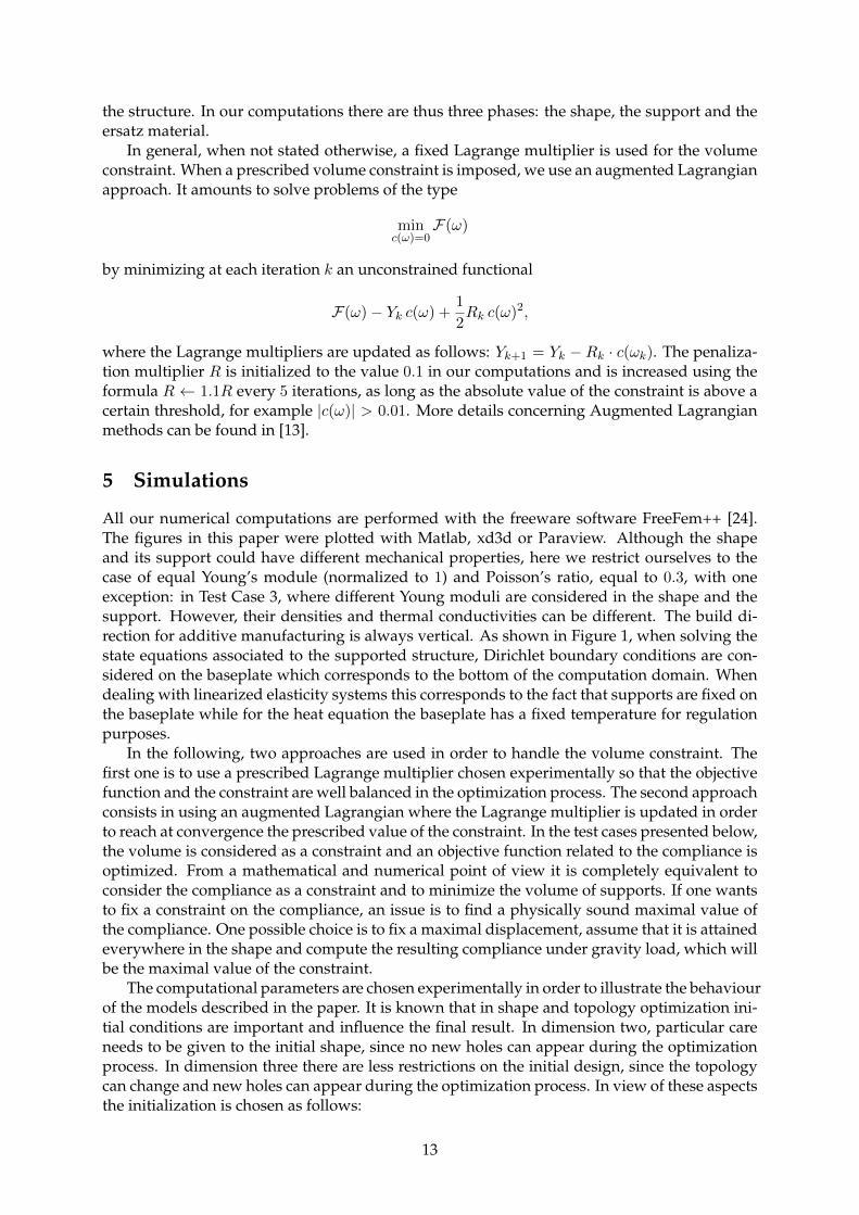
In general, when not stated otherwise, a fixed Lagrange multiplier is used for the volumeconstraint. When a prescribed volume constraint is imposed, we use an augmented Lagrangianapproach. It amounts to solve problems of the type

minc(ω)=0

F(ω)

by minimizing at each iteration k an unconstrained functional

F(ω)− Yk c(ω) +1

2Rk c(ω)2,

where the Lagrange multipliers are updated as follows: Yk+1 = Yk − Rk · c(ωk). The penaliza-tion multiplier R is initialized to the value 0.1 in our computations and is increased using theformula R ← 1.1R every 5 iterations, as long as the absolute value of the constraint is above acertain threshold, for example |c(ω)| > 0.01. More details concerning Augmented Lagrangianmethods can be found in [13].

5 Simulations

All our numerical computations are performed with the freeware software FreeFem++ [24].The figures in this paper were plotted with Matlab, xd3d or Paraview. Although the shapeand its support could have different mechanical properties, here we restrict ourselves to thecase of equal Young’s module (normalized to 1) and Poisson’s ratio, equal to 0.3, with oneexception: in Test Case 3, where different Young moduli are considered in the shape and thesupport. However, their densities and thermal conductivities can be different. The build di-rection for additive manufacturing is always vertical. As shown in Figure 1, when solving thestate equations associated to the supported structure, Dirichlet boundary conditions are con-sidered on the baseplate which corresponds to the bottom of the computation domain. Whendealing with linearized elasticity systems this corresponds to the fact that supports are fixed onthe baseplate while for the heat equation the baseplate has a fixed temperature for regulationpurposes.

In the following, two approaches are used in order to handle the volume constraint. Thefirst one is to use a prescribed Lagrange multiplier chosen experimentally so that the objectivefunction and the constraint are well balanced in the optimization process. The second approachconsists in using an augmented Lagrangian where the Lagrange multiplier is updated in orderto reach at convergence the prescribed value of the constraint. In the test cases presented below,the volume is considered as a constraint and an objective function related to the compliance isoptimized. From a mathematical and numerical point of view it is completely equivalent toconsider the compliance as a constraint and to minimize the volume of supports. If one wantsto fix a constraint on the compliance, an issue is to find a physically sound maximal value ofthe compliance. One possible choice is to fix a maximal displacement, assume that it is attainedeverywhere in the shape and compute the resulting compliance under gravity load, which willbe the maximal value of the constraint.

The computational parameters are chosen experimentally in order to illustrate the behaviourof the models described in the paper. It is known that in shape and topology optimization ini-tial conditions are important and influence the final result. In dimension two, particular careneeds to be given to the initial shape, since no new holes can appear during the optimizationprocess. In dimension three there are less restrictions on the initial design, since the topologycan change and new holes can appear during the optimization process. In view of these aspectsthe initialization is chosen as follows:

13

• dimension 2: the initial design is chosen as either the complement of a union of equallyspaced disks corresponding to vertically aligned holes, or as the level-set given by anexpression coming from a product of cosines of the form cos(2nπx) cos(2nπy) − 0.5, cor-responding to diagonally aligned holes. The parameter n controls the number of holes inthe second case. For the two dimensional computations, the initializations are displayedor explicitly referenced.• dimension 3: the initial condition is chosen as full subset or as the whole computational

domain. In some cases some balls may be removed in order to enrich the topology of thefinal result. In each of the computations below we describe the initialization used in thecomputations.

The computational time depends on the dimension, on the size of the discretization andon the number of optimization iterations. For example, performing 300 iterations for the twodimensional computations presented in the Test Cases 1 and 2 below takes less than half anhour. For the three dimensional computations with 150 iterations the computational time isaround three hours for both Test Cases 5 and 6 when dealing with roughly 105 degrees offreedom. The computations were made on an Intel Xeon 8 core processor, with 32 RAM and onan Intel i7 quad-core laptop with 16GB of RAM.

5.1 Minimizing Compliance with a Fixed Shape

In this subsection the shape ω is fixed and we only optimize the support S for minimal compli-ance under gravity loads (see Subsection 2.1). In all the following cases we take g = (0,−1) indimension two and g = (0, 0,−1) in dimension three.

Test Case 1 (MBB beam). The fixed shape ω is a MBB beam obtained by compliance minimizationfor a volume V = 1.13, without any further constraint (see e.g. [4] for details). The fixed shape, theinitial and optimal supports are shown in Figure 2. Gravity does not apply to the support S, namelyρS = 0. The supports are obtained for the density ρω = 2.5 and the optimization procedure has 300iterations. The computational domain is of size 3× 1 corresponding to half of the beam and a symmetrycondition on the vertical symmetry axis is imposed by making the horizontal displacement equal to zero.The computational domain D is discretized using a grid of size 301 × 101 with 30401 nodes and P1

finite elements are used for solving (2). In this simulation the support and the fixed shape have the samemechanical parameters.

Figure 2: The fixed shape and the initialization used for Test Case 1 (MBB beam).

In order to illustrate the behaviour of the algorithm two versions of the optimization proce-dure are used here: fixed Lagrange multiplier (Figure 3) and augmented Lagrangian (Figure 4).The initial condition is the same and the target volume for the augmented Lagrangian is chosenas the final volume of the structure obtained at the end of the optimization with fixed Lagrangemultiplier. Note the differences in the convergence histories between the two algorithms. Con-vergence is monotone for all terms in the optimization process with a fixed Lagrange multiplier.On the other hand, with the augmented Lagrangian approach, compliance first increase until

14

Figure 3: Optimal supports and convergence curves for Test Case 1 with a fixed Lagrangemultiplier ` = 1. Fixed shape and initialization given in Figure 2

Figure 4: Optimal supports and convergence curves for Test Case 1 with a volume constraintand an augmented Lagrangian algorithm. Fixed shape and initialization given in Figure 2

the volume constraint is satisfied, and later it decreases. The final volume of the support struc-ture is 0.4620 and the final compliances are 1.4648 for the fixed Lagrange multiplier and 1.4330for the augmented Lagrangian approach. The augmented Lagrangian approach finds a struc-ture which performs better and is topologically different from the one obtained with a fixedLagrange multiplier, starting from the same initial condition and using the same mechanicalparameters.

The interest of Test Case 1 is that the initial MBB beam has large horizontal parts. Thesehorizontal parts cannot be produced using additive manufacturing processes, unless they aresupported. Notice that the optimal support S is distributed in such a way that overhang re-gions are indeed supported. Moreover, the results obtained with our algorithm resemble thosepresented in [4], where the additive manufacturing constraints imposed in the optimizationprocess lead to a self-supporting structure.

In order to evaluate the performance of the support with respect to its volume constraint,we plot in Figure 5 the computed optimal compliances as a function of the support volume. Asexpected, the optimal compliance is decreasing with respect to the volume constraint. A smallamount of support improves a lot the rigidity of the supported structure, but the improvementis saturating when adding more and more supports.

Test Case 2 (M-shape). The fixed shape and the initial and optimal support are displayed in Figure 6.

15

Figure 5: Optimal compliance of the supported structure as a function of the support volumeconstraint for Test Case 1.

Figure 6: Numerical results for Test Case 2. From left to right, fixed M-shape, initial and finalsupports.

The M-shape consists of two thin vertical bars, connected by a thicker part. The computational domainhas size 3.1× 3 and the mesh has 156× 151 degrees of freedom. We consider ρω = 5 for the fixed shapeand we optimize the objective function (4) with a fixed Lagrange multiplier ` = 150. The convergencehistory of the algorithm for 300 iterations can be seen on Figure 7.

The motivation for Test Case 2 comes from the fact the M-shape successfully passes thegeometric constraint of an angle between the boundary normal and the build direction lessthan 45 degrees, although the overall structure is clearly overhanging. Such a M-shape is hardto manufacture without support since the lower angle of the M start right in the middle of thepowder bed. Thus it requires some support. Moreover, in order to have the desired stabilityas the layers are added, the support should be strong enough to hold the start surface and thesubsequent layers, until they join with the other parts of the structure. With our model, optimalsupports distribute as expected in order to provide enough resistance for the part of the shapewhich starts to be fabricated from the powder bed.

Test Case 3 (MBB beam with different phases). In order to illustrate the behavior of the algorithmwhen different mechanical parameters are present in the shape and the support, the same configurationas in Test Case 1 is considered, but the support is allowed to have different material properties from theshape. In this case the mesh has 301× 101 nodes. The Young modulus of the shape is set to be equal to 1,while the Young modulus of the support has the values 0.5, 0.9 and 1. The optimization algorithm usesan augmented Lagrangian approach and the combined volume of the shape and support is set to convergeto 1.7. Results, histories of convergence and final values of the compliances can be visualized in Figure8.

The goal of Test Case 3 is to test the influence of a different stiffness of the support withrespect to the shape. As expected, supports tend to be more massive when its Young modulusis smaller. Since the same initial condition is used for all three computations, the topological

16

Figure 7: Convergence history of the cost function, the volume and the compliance for TestCase 2 (M-shape).

structure of the result is not radically different in the result. Nevertheless, the convergencecurves for the compliances which can be seen in Figure 8 show that the stiffness of the sup-ported structure decreases when weaker materials are used for supports.

The goal of the next computation is to make a comparison between our model and the onepresented by Kuo et al. in [30] which does not feature the same loading conditions. Theirsurface loads are reproduced in Figure 9 and compared to the bulk loads which are used in thiswork. Recall that in [30] the authors also used techniques in order to facilitate the removal ofsupports and that these ideas are not implemented in the models proposed here.

Test Case 4 (Kuo et al.). The fixed shape is represented in Figure 9. Since the model used in [30]is different from the ones proposed in this article, two loading cases are considered: one surface loadcorresponding to the model in [30] and one bulk load corresponding to the model proposed in Section2.1. The optimization is done with an augmented Lagrangian approach with target volume 0.7 for thecombined structure part/supports. The parameters considered are ρω = 2, ρS = 0. The initial designand the optimized ones for each of the loading cases are shown in Figure 9. In view of the fact that themesh and shape parameters, loading cases and mechanical properties are not the same in the two models,no precise quantitative comparison of the results can be made. From a qualitative point of view, it canbe noted that when using volumic forces, supports tends to concentrate under the more massive parts ofthe structure. The model proposed in [30] allows a more uniform distribution of supports, but for moregeneral and complex shapes it is not clear on which surfaces should the surface load be applied.

Test Case 5 (3D chair). The fixed shape and the optimal support are displayed on Figure 10. Thecomputational domain is the union of the rectangular boxes [0, 6]×[0, 2]×[0, 6] and [0, 2]×[0, 2]×[6, 12].The domain is meshed using 343201 nodes. The initial support fills the whole domain outside the shape.The density is ρω = 3.7, the volume of the chair structure represents 5% of the computational domainand the Lagrange multiplier is chosen so that the final volume of the support is 3% of the volume of thecomputational domain. The optimization procedure has 150 iterations.

Test Case 5 is inspired from [7], where the 3D chair shape was obtained by complianceminimization.

Test Case 6 (3D beam). The fixed shape and the optimal support are displayed on Figure 11. Dueto the symmetry we work on a quarter of the box containing the shape. The computational domain is[0, 3] × [0, 0.5] × [0, 1] which is discretized using finite elements. The discretization contains 104181nodes and 576000 tetrahedra. The density is ρω = 3.5 in the fixed shape and we adapt the Lagrangemultiplier in order that the final support occupies 4% of the computational box (equal to 0.24). The opti-mization procedure has 300 iterations. The fixed MBB beam was obtained by compliance minimizationand occupies 10% of the computational domain. The initial support, the result of the optimization and theconvergence histories are represented in Figure 11. Note that these graphs correspond to computationsmade on one quarter of the domain with symmetry conditions.

17

Figure 8: Test Case 3: optimal supports and convergence histories obtained when varying theYoung modulus of the support. The Young modulus of the support is equal to 1, 0.9 and 0.5(from top to bottom), while for the shape it is kept at 1.

Figure 9: (top row) Loadings considered for the Test Case 4 inspired from [30]. On the left, bulkloads as proposed in the present work, while on the right, for the sake of comparison, surfaceloads as proposed in [30]. (bottom row): initial support (left), result for the model proposedin this article using bulk loads (center), result for the model using surface loads on the upperboundary as in [30] (right).

18

Figure 10: Test Case 5 (3D chair): fixed shape (left) and two views of the optimal supports.

Figure 11: Test Case 6 (3D beam): fixed shape and initial (left) and the optimized support (right)together with the convergence curves.

In order to automatically generate support structures, most commercial or proprietary soft-wares propose methods based on geometric criteria. One such criterion is to detect all surfaceswhich are sufficiently close to being horizontal. An inclination angle α0 is given and it is de-cided that all structure boundaries which make an angle smaller than α0 with the horizontalplane have to be supported. We implemented this simple idea and define vertical supportsunder all overhanging regions given by the angle α0. In the following, the case of the 3D MBBBeam is studied and supports are calculated for multiple values of α0. In the left column ofFigure 12 our results, obtained for α0 ∈ 21.5, 30, 45, are provided. The corresponding sup-port volumes are 0.24, 0.48 and 0.80, respectively. In particular, note that the solution obtainedfor α0 = 21.5 has the same volume as the one used as a target in the Test Case 6. In view of theresults presented in Figure 11, this kind of supports based on simple geometric assumptionscan be further optimized, showing again the interest in modeling the optimization of supports.

For the sake of comparison, the free software Ultimaker Cura1 was also used in order to

1Webpage: https://ultimaker.com/en/products/ultimaker-cura-software

19

Figure 12: (left) Vertical supports generated under the overhang regions for the fixed beamshape shown in Figure 11 for limiting angle α0 ∈ 21.5, 30, 45. (right) Supports generatedby the freeware software Ultimaker Cura for the same angles.

generate supports for the same angles α0 as above. The resulting support structures, generatedwith default parameters of the software, are shown in the right column of Figure 12 for aneasy comparison with our results, obtained with the simple geometrical method described inthe previous paragraph. Clearly the supports of both columns of Figure 12 are qualitativelysimilar, which is a confirmation that only geometric information is used to generate supportsin Ultimaker Cura.

5.2 Thermal evacuation

In the following, results obtained for the optimization of supports for heat evacuation are pre-sented. The theoretical aspects concerning the objective functions and shape derivatives usedcan be found in Subsection 3. The heat equation (11) with a constant source term f in the fixedshape ω is considered and the support structure S is optimized such that the thermal compli-ance is minimized. In practice, this would correspond to an optimal evacuation or regulation ofthe heat produced by the additive manufacturing process. In the following test cases a Dirich-let condition T = 0 is imposed on some parts of the boundary of the computational domain.It is expected that supports will connect the shape ω to these parts of the boundary. Since theconductivity of the powder is orders of magnitude smaller than the conductivity of the shapeor the support, Neumann boundary conditions are imposed on ∂(S ∪ ω). Here, only simpletest cases in dimension two are performed. More complex situations can be handled with noadditional difficulties: for example, different thermal conductivities in the structure and thesupport, non-constant source terms, etc.

In this subsection, the fixed shape ω is a cantilever, obtained by compliance minimizationwith volume 0.8 in a 2× 1 rectangular box with a vertical point load at the middle of the rightside and a clamped left side. In all the test cases of this subsection the optimization procedurehas 300 iterations.

Test Case 7. A cantilever shape is considered in a 2 × 1 rectangular box with Dirichlet condition onthe baseplate (bottom of the domain). The conductivity in the fixed shape and the support is set to 0.5and the constant source term f is equal to 2 in the fixed shape. The optimization is done using anaugmented Lagrangian method: the final support has volume 0.35. The initialization and the result ofthe optimization can be seen in Figure 13.

In industrial practice only connections to the baseplate (lower boundary) of the build cham-

20

ber can be considered as solid contact, which could efficiently evacuate the heat. Nevertheless,the next test case investigates other boundaries where to apply Dirichlet boundary condition,for the sake of comparison and since the role of supports for heat evacuation is still in debate.Note also that supports are often used to connect the structure to the baseplate: thus, contrarilyto the Test Case 7, the structure is placed slightly above the baseplate so that supports must ap-pear between the structure and the baseplate. It is thus not surprising that the optimal supportsare different between Test Cases 7 and 8.

Test Case 8. In this test case the behaviour of the algorithm with respect to different boundary conditionsis investigated. In Figure 14 a slightly enlarged box of size 2.2× 1.2 is considered around the cantileverand it is placed such that it is not in contact with any of the boundaries. In this case the behavior of thealgorithm with respect to different boundary conditions is investigated. As expected, supports optimizedin order to reduce the temperature tend to connect to the parts of the boundary which are regulatedthrough the Dirichlet boundary condition.

Figure 13: Test Case 7: initial and optimal supports for thermal evacuation.

Figure 14: Test Case 8: Optimal supports for thermal evacuation with different boundary con-ditions: bottom, top-bottom, top-bottom-right and left-right.

Test Case 9. In order to optimize the behavior of the structure concerning the heat evacuation, themaximization of the fundamental eigenvalue of the system given in (14) is considered. The conductivitiesare set to 0.5 and the density is ρω = 1. Dirichlet boundary conditions are imposed on the lowerboundary of the domain. The optimization is done using an augmented Lagrangian method: the finalsupport has volume 0.35. The initial support is the same as the one in Test Case 7 and is shown in Figure13. The result of the optimization is presented in Figure 15.

The optimal support of Test Case 9 is quite similar to that of Test Case 7 which indicatessome kind of robustness of this design to the chosen model.

21

Figure 15: Test Case 9: Maximization of the first eigenvalue for the heat equation.

5.3 Mixing elastic and thermal constraints

We now consider an objective function which takes into account both mechanical and thermalconstraints: the average of the elastic and thermal compliances. In order to perform the opti-mization, one simply needs to solve both the elastic system (2) and the thermal system (11) andcombine the corresponding shape derivatives.

Test Case 10. The fixed shape is a MBB beam (same as in Test Case 1). The parameters are as follows.The mesh consists of a 301 × 101 grid which is triangulated, representing half the beam, by symmetry.The source is 2.5 in the beam and the conductivity is k = 0.5χω + χS . The mechanical parameters arethe same as in other computations in the previous subsection: Young modulus is 1 and the Poisson ratiois 0.3. A fixed Lagrange multiplier ` = 1 is used and the optimization procedure has 300 iterations. Theoptimal supports obtained are shown in Figure 16. The initial support is initialized with a grid of 15× 4vertically aligned holes.

Figure 16: Test Case 10: Optimal supports with respect to the average of mechanical and ther-mal compliances.

5.4 Simultaneous optimization of the shape and the support

Following the theoretical results stated in Section 2.2, the optimization of the shape and thesupport at the same time is illustrated below. The difficulty here is to be able to represent nu-merically both the shape and the support and to evolve through the Hamilton-Jacobi equationthe corresponding parts of ∂ω and ∂S following the derivatives given in equations (8). In or-der to represent both the fixed shape ω and the support S and to distinguish easily betweenboundaries ∂ω \ ∂S, ∂S \ ∂ω and ∂ω ∩ ∂S, two level set functions are used, following classicalideas from [44], [45]. These techniques were already used when dealing with the optimizationof structures made of multiple materials in [3]. In our case two level sets ψ1, ψ2 : D → R areneeded. The mechanical shape ω and the support S are represented with the aid of the level-setfunctions ψ1, ψ2 as follows

x ∈ ω ⇔ ψ1(x) ≤ 0x ∈ S ⇔ ψ1(x) > 0 and ψ2(x) ≤ 0

x ∈ D \ (ω ∪ S) ⇔ ψ1(x) > 0 and ψ2(x) > 0.

22

Figure 17: Test Case 11: Simultaneous optimization of a MBB beam and its supports togetherwith the initialization of the two level sets used to represent S and ω.

This helps decide how to implement the shape derivatives formulas found in (8). The vectorfield θ, giving a descent direction, is chosen as follows

x ∈ ∂ω \ ∂S ⇔ ψ1(x) = 0 and ψ2(x) > 0 ⇒ θ(x) = −j1(x)nx ∈ ∂ω ∩ ∂S ⇔ ψ1(x) = 0 and ψ2(x) ≤ 0 ⇒ θ(x) = −j2(x)nx ∈ ∂S \ ∂ω ⇔ ψ1(x) = 0 and ψ2(x) > 0 ⇒ θ(x) = −j3(x)n,

where the expressions of j1, j2 and j3 can be found in (8) and n is the normal vector to the con-sidered surfaces. On ∂ω∩∂S the normal vector n is chosen pointing outwards ω. In view of theshape derivative formulas (8) the choice of a vector field perturbation θ gives a correspondingdescent direction for the functional we wish to optimize. The volume constraints on ω and Sare implemented via Lagrange multipliers. In order to allow different behaviors concerningthe shape or the support, two different Lagrange multipliers `ω, `S are used and the functionalto be optimized is the following:

J2(ω, S) + `ωVol(ω) + `SVol(S) =

∫Γ0

ffin ·ufin ds+

∫ω∪S

ρg ·uspt dx+ `ωVol(ω) + `SVol(S). (17)

The initialization for the two level sets ψ1, ψ2 needs also particular care. In order to haverich enough structures for the shape and the support one should place the holes such that theboundaries of S and ω do not coincide so that the shape derivatives corresponding to parts∂ω \ S, ∂ω ∩ ∂S and ∂S \ ∂ω are all active. An example of initialization is given in Figure 17.

Test Case 11. We minimize (17) simultaneously with respect to S and ω. In Figure 17 the initialconfiguration of the two level sets, as well as the result of the optimization algorithm are displayed (seethe previous paragraph for a justification of the choice of the initial support and shape). The MBB-beamis optimized under a standard center load with sliding boundary conditions at the lower corners and thesupport is optimized under the gravity loads of the beam. The Lagrange multipliers are `ω = 1.4 for thebeam and `S = 0.5 for the support. The vertical load for the mechanical properties of the final shape isequal to ffin = 2.5ed and the density of the shape used in (2) is ρω = 2.5 (ρS = 0). The optimizationprocedure took 200 iterations.

5.5 Towards an optimized orientation

In practice when given a shape ω to be printed, before searching for a support strategy oneneeds to find the proper orientation of the shape which ensures that the need for supports isminimal. In the following, our algorithm is applied to a fixed cantilever shape under differentorientations. The capabilities of FreeFem++ [24] are used in order to rotate the level set andconstruct a new mesh containing it so that the quality of the level set function is preserved

23

Figure 18: Convergence history of the volume and compliance when optimizing the supportsfor the horizontal orientation of the cantilever presented in Figure 19. The volume constraint isimplemented using an augmented Lagrangian approach.

under rotation. We perform the exact rotation of the mesh using the command movemesh withthe vector-field

Φ = (x cosα− y sinα, x sinα+ y cosα),

corresponding to an exact rotation of angle α. In this way, a new rectangular mesh containingthe rotated shape is constructed and the level set is interpolated on this new mesh. Further-more, the mesh is truncated so that the unnecessary parts of the mesh which lie above therotated shape are not considered in the computation. Finally, the width of the mesh coincideswith the width of the rotated shape.

Optimized supports for a cantilever shape under different orientations are presented below.The minimal compliance model presented in Section 2 is used in order to optimize the supportsin this case. The results given in Figure 19 correspond to rotation angles 0, 30, 45, 60 and90. More precisely, the compliance of the structure ω ∪ S, given by (3), is optimized with afixed volume constraint, implemented as an augmented Lagrangian. The convergence curvesfor the volume, compliance and the cost function are shown in Figure 18, noticing that we havethe desired convergence of the volume. Various computations are performed for all angles,multiples of 7.5, between 0 and 90 for different volume constraints and the final complianceof the structure for each angle is represented in Figure 20. For comparison, the compliance ofthe structure without supports is also presented. Of course, compliance is greatly diminishedwhen adding supports. The behavior of compliance with respect to the support volume is alsoindicated by three different curves. Again, compliance is decreased by adding more supports.It is striking to check that, without support, the minimal compliance is obtained for the verticalorientation of the cantilever, while, with support, it is the horizontal orientation which yieldsthe smallest compliance (whatever the tested volume of support).

Figure 19: Optimal supports for different orientations 0, 30, 45, 60 and 90 of the fixedshape. The support has fixed volume in all computations. The cantilever shapes have thesame size, but the pictures are rescaled to have a fixed height.

Remark 5.1. The computations described above were made for a fixed family of angles. An immediateperspective of this work is to consider the angle as a parameter in the optimization process. The sensitivity

24

Figure 20: Final compliance of the structure ω ∪ S with respect to the orientation angle for therotated cantilevers in Figure 19. Different curves correspond to different volume constraintsfor the support.

with respect to the angle parameter is classical. However, there are some choices regarding the couplingbetween the support and the rotated shape. Either the shape and its support are rotated together or theshape is rotated, while the support remains fixed. We favor the last choice, but close attention needs to begiven in order to prevent the separation of the structure and its support.

5.6 Layer by layer model

In the following, results concerning the minimization of the functional (10), which models thelayer by layer AM process, are presented (see Section 2.3 for details and notations). Recall thatthe number of layers, denoted by N , is much smaller in our model than in reality, for mini-mizing the computational cost. Given the computational domain D and the number of slices,meshes are constructed for D and for each region Di = D ∩ xd ≤ hi. In order to computethe objective function modeling the layer by layer process (10), N partial differential equationsof the type (9) need to be solved. Ideally, the mesh chosen in the whole computational domainD will have meshes Di as sub-meshes which will be computed only once, before starting theoptimization algorithm in FreeFem++. Each of the solutions ui is then interpolated on D by ex-tending it with zero on the region xd > hi. The extensions of u from Di to D are denoted byui. Finally, the vector field giving the descent direction for the level set optimization algorithm,is be given by

θ = −N∑i=1

(−Ae(ui) · e(ui) + 2fi · ui)n,

where n is the normal vector to ∂S.

Test Case 12. In dimension two the MBB beam structure is used (same as in Test Case 1) and theobjective function (10) is minimized for 10 and 50 slices. Shape optimization problems tend to havemultiple local minima, therefore the solution found by the optimization algorithm depends on the initialchoice. The results of the optimization algorithm for two different initializations are shown in Figure 21.The computation is made for a fixed volume constraint and comparing the final costs given by (10) it canbe noticed that structures corresponding to the vertical alignment of holes in the initial condition give aslightly lower cost function. The mechanical parameters and the fixed beam are the same as in Test Case1. The optimization algorithm takes 150 iterations.

25

Figure 21: Test Case 12: Optimization of the supports for a MBB beam for 10 (middle line) and50 slices (bottom line), for different initial conditions at fixed volume (top line). The optimizeddesigns on the left, giving rise to vertical bar structures, have a lower value of the cost function.

Figure 22: Test Case 13: Optimization of the supports for the 3D chair structure for 5, 10 and 20slices.

A strong resemblance between our results and the self supporting structures obtained in[4], [5] can be observed.

Test Case 13. In dimension three the layer by layer algorithm is applied to the chair structure usedbefore in the Test Case 5 for 5, 10 and 20 slices. The mechanical and optimization parameters are thesame. The results obtained are shown in Figure 22. As the number of slices increases, it can be noticedthat the structure of supports modifies slightly so that there is a more uniform supporting of overhangsurfaces.

The computational cost for the layer by layer model is important since we need to solve thestate equation for each slice. In general, for N slices, the computational cost is multiplied byN , since most of the time in the optimization algorithm is spent solving the elasticity systems.Two dimensional computations for 50 slices take about 3 hours, while the three dimensionalcomputations for 20 slices took 2 days of computational time.

26

6 Conclusion

This paper introduces several models and algorithms for the optimization of supports in addi-tive manufacturing. Our mathematical models are based on the mechanical and thermal prop-erties regarding the combined structure shape/support. Yet, they are simple enough so thattheir computational cost remains reasonable. They allow to successfully detect and supportoverhang regions without relying only geometrical information. We also consider the simul-taneous optimization of the shape and its support in a multiphase optimization framework.The numerical computations were performed with the freeware software FreeFem++ [24], inreasonable computational times. For example a typical 2-d optimization with 300 iterations ona mesh of size 300× 100 takes less than half an hour on a laptop (Intel i7 quad-core laptop with16GB of RAM), while a 3-d optimization with 150 iterations on a mesh consisting of around105 nodes costs around 3 hours of CPU time. We believe that our algorithms, coupled withmore optimized finite element solvers (for example, using parallel computing), could be easilyimplemented and used for industrial purposes. A parallel version of our algorithm is a workin progress and it could significantly improve computational times in dimension three. In afuture work we plan to handle the optimization of the shape orientation, combined with thatof the supports. We also want to incorporate other manufacturability constraints, includingaccessibility issues related to the removal of supports. The removal of supports may pose diffi-culties, especially for complex 3-d shapes. To guarantee the ease of removal, any contact zonebetween supports and the actual shape should be accessible from the outside along a straightline. This can be added as a constraint in the optimization process. Another constraint relevantto supports is the penalization of the unnecessary contact zone between the support and theshape. The optimal orientation with respect to the area of overhang regions and the volumeunder overhang regions is also a relevant aspect regarding the support structures. All these is-sues are the topic of an ongoing work. Of course, it is crucial to assess our optimized supportswith experiments. This will be the topic of a future collaboration with industrial partners inthe SOFIA project.

Acknowledgements

This work was partially supported by the SOFIA project, funded by BPI (Banque Publiqued’Investissement). G.A. is a member of the DEFI project at INRIA Saclay Ile-de-France.

References

[1] G. Allaire. Conception optimale de structures, volume 58 of Mathematiques & Applications(Berlin) [Mathematics & Applications]. Springer-Verlag, Berlin, 2007.

[2] G. Allaire. Numerical analysis and optimization. Numerical Mathematics and Scientific Com-putation. Oxford University Press, Oxford, 2007. An introduction to mathematical mod-elling and numerical simulation, Translated from the French by Alan Craig.

[3] G. Allaire, C. Dapogny, G. Delgado, and G. Michailidis. Multi-phase structural optimiza-tion via a level set method. ESAIM Control Optim. Calc. Var., 20(2):576–611, 2014.

[4] G. Allaire, C. Dapogny, R. Estevez, A. Faure, and G. Michailidis. Structural optimizationunder overhang constraints imposed by additive manufacturing technologies. J. Comput.Phys., 351:295–328, 2017.

[5] G. Allaire, C. Dapogny, A. Faure, and G. Michailidis. Shape optimization of a layerby layer mechanical constraint for additive manufacturing. C. R. Math. Acad. Sci. Paris,355(6):699–717, 2017.

27

[6] G. Allaire and L. Jakabcin. Taking into account thermal residual stresses in topology op-timization of structures built by additive manufacturing. M3AS, to appear. preprint hal-01666081.

[7] G. Allaire and F. Jouve. A level-set method for vibration and multiple loads structuraloptimization. Computer methods in applied mechanics and engineering, 194(30):3269–3290,2005.

[8] G. Allaire, F. Jouve, and G. Michailidis. Molding direction constraints in structural opti-mization via a level-set method. In Variational analysis and aerospace engineering, volume116 of Springer Optim. Appl., pages 1–39. Springer, Cham, 2016.

[9] G. Allaire, F. Jouve, and G. Michailidis. Thickness control in structural optimization via alevel set method. Struct. Multidiscip. Optim., 53(6):1349–1382, 2016.

[10] G. Allaire, F. Jouve, and A.-M. Toader. Structural optimization using sensitivity analysisand a level-set method. J. Comput. Phys., 194(1):363–393, 2004.

[11] C. Barlier and A. Bernard. Fabrication additive - Du Prototypage Rapide a l’impression 3D.Dunod, Paris, 2016.

[12] M. P. Bendsøe and O. Sigmund. Topology Optimization. Springer Berlin Heidelberg, 2004.

[13] E. G. Birgin and J. M. Martınez. Practical augmented Lagrangian methods for constrained op-timization, volume 10 of Fundamentals of Algorithms. Society for Industrial and AppliedMathematics (SIAM), Philadelphia, PA, 2014.

[14] M. Bruggi, N. Parolini, F. Regazzoni, and M. Verani. Finite element approximation of anevolutionary topology optimization problem. Additive Manufacturing, 12(Part A):60 – 70,2017.

[15] C. Bui, C. Dapogny, and P. Frey. An accurate anisotropic adaptation method for solvingthe level set advection equation. Internat. J. Numer. Methods Fluids, 70(7):899–922, 2012.

[16] S. Cacace, E. Cristiani, and L. Rocchi. A level set based method for fixing overhangs in 3Dprinting. Appl. Math. Model., 44:446–455, 2017.

[17] F. Calignano. Design optimization of supports for overhanging structures in aluminiumand titanium alloys by selective laser melting. Materials & Design, 64:203–213, 2014.

[18] J. Cea. Conception optimale ou identification de formes: calcul rapide de la derivee direc-tionnelle de la fonction cout. RAIRO Model. Math. Anal. Numer., 20(3):371–402, 1986.

[19] C. Dapogny and P. Frey. Computation of the signed distance function to a discrete contouron adapted triangulation. Calcolo, 49(3):193–219, 2012.

[20] J. Dumas, J. Hergel, and S. Lefebvre. Bridging the gap: Automated steady scaffoldings for3d printing. ACM Trans. Graph., 33(4):98:1–98:10, July 2014.

[21] M. Gan and C. Wong. Practical support structures for selective laser melting. Journal ofMaterials Processing Technology, 238:474 – 484, 2016.

[22] N. Gardan and A. Schneider. Topological optimization of internal patterns and support inadditive manufacturing. Journal of Manufacturing Systems, 37:417 – 425, 2015.

[23] I. Gibson, D. Rosen, and B. Stucker. Additive Manufacturing Technologies. Springer NewYork, 2015.

28

[24] F. Hecht. New development in FreeFem++. J. Numer. Math., 20(3-4):251–265, 2012.

[25] A. Henrot and M. Pierre. Variation et optimisation de formes, volume 48 of Mathematiques &Applications (Berlin) [Mathematics & Applications]. Springer, Berlin, 2005.

[26] K. Hu, S. Jin, and C. C. Wang. Support slimming for single material based additive man-ufacturing. Computer-Aided Design, 65:1 – 10, 2015.

[27] X. Huang, C. Ye, S. Wu, K. Guo, and J. Mo. Sloping wall structure support generation forfused deposition modeling. The International Journal of Advanced Manufacturing Technology,42(11):1074, Aug 2008.

[28] A. Hussein, L. Hao, C. Yan, R. Everson, and P. Young. Advanced lattice support structuresfor metal additive manufacturing. Journal of Materials Processing Technology, 213(7):1019 –1026, 2013.

[29] Y.-H. Kuo, C.-C. Cheng, Y.-S. Lin, and C.-H. San. Support structure design in additivemanufacturing based on topology optimization. Struct. Multidiscip. Optim., 57(1):183–195,2018.

[30] Y.-H. Kuo, C.-C. Cheng, Y.-S. Lin, and C.-H. San. Support structure design in additivemanufacturing based on topology optimization. Struct. Multidiscip. Optim., 57(1):183–195,2018.

[31] M. Langelaar. Topology optimization of 3d self-supporting structures for additive manu-facturing. Additive Manufacturing, 12(Part A):60 – 70, 2016.

[32] M. Langelaar. Combined optimization of part topology, support structure layout and buildorientation for additive manufacturing. Structural and Multidisciplinary Optimization, Jan2018. doi: 10.1007/s00158-017-1877-z.

[33] M. Leary, L. Merli, F. Torti, M. Mazur, and M. Brandt. Optimal topology for additive man-ufacture: A method for enabling additive manufacture of support-free optimal structures.Materials & Design, 63(Supplement C):678–690, 2014.

[34] F. Mezzadri, V. Bouriakov, and X. Qian. Topology optimization of self-supporting supportstructures for additive manufacturing. Additive Manufacturing, 21:666–682, may 2018.

[35] G. Michailidis. Manufacturing Constraints and Multi-Phase Shape and Topology Opti-mization via a Level-Set Method. PhD thesis, Ecole Polytechnique, 2014, available at:http://pastel.archives-ouvertes.fr/pastel-00937306.

[36] A. M. Mirzendehdel and K. Suresh. Support structure constrained topology optimizationfor additive manufacturing. Computer-Aided Design, 81:1 – 13, 2016.

[37] H. D. Morgan, J. A. Cherry, S. Jonnalagadda, D. Ewing, and J. Sienz. Part orientationoptimisation for the additive layer manufacture of metal components. The InternationalJournal of Advanced Manufacturing Technology, 86(5):1679–1687, Sep 2016.

[38] K. Mumtaz, P. Vora, and N. Hopkinson. A method to eliminate anchors/supports from di-rectly laser melted metal powder bed processes. Proc. Solid Freeform Fabrication Symposium,Sheffield, pages 54–64, 2011.

[39] S. Osher and R. Fedkiw. Level set methods and dynamic implicit surfaces, volume 153 ofApplied Mathematical Sciences. Springer-Verlag, New York, 2003.

[40] O. Pironneau. Optimal shape design for elliptic systems. Springer Series in ComputationalPhysics. Springer-Verlag, New York, 1984.

29

[41] J. A. Sethian. Level set methods and fast marching methods, volume 3 of Cambridge Monographson Applied and Computational Mathematics. Cambridge University Press, Cambridge, sec-ond edition, 1999.

[42] G. Strano, L. Hao, R. M. Everson, and K. E. Evans. A new approach to the design andoptimisation of support structures in additive manufacturing. The International Journal ofAdvanced Manufacturing Technology, 66(9):1247–1254, Jun 2013.

[43] J. Vanek, J. A. G. Galicia, and B. Benes. Clever support: Efficient support structure gener-ation for digital fabrication. Computer Graphics Forum, 33(5):117–125, 2014.

[44] L. Vese and T. Chan. A multiphase level set framework for image segmentation using themumford and shah model. Int. J. Comput. Vision, 50 (3):271–293, 2002.

[45] M. Y. Wang and X. Wang. “Color” level sets: a multi-phase method for structural topologyoptimization with multiple materials. Comput. Methods Appl. Mech. Engrg., 193(6-8):469–496, 2004.

[46] X. Zhang, X. Le, A. Panotopoulou, E. Whiting, and C. C. L. Wang. Perceptual models ofpreference in 3d printing direction. ACM Trans. Graph., 34(6):215:1–215:12, Oct. 2015.

30