Optimizing Diesel Fuel Supply Chain Operations for Hurricane Relief

Daniel Duquea, Haoxiang Yangb and David P. Mortona

aDepartment of Industrial Engineering & Management Sciences, Northwestern University,Evanston, IL, USA; bCenter for Nonlinear Studies, Los Alamos National Laboratory, LosAlamos, NM, USA

ARTICLE HISTORY

Compiled May 10, 2020

ABSTRACTHurricanes can cause severe property damage and casualties in coastal regions. Dieselfuel plays a crucial role in hurricane disaster relief. It is important to optimize fuelsupply chain operations so that emergency demand for diesel can be mitigated in atimely manner. However, it can be challenging to estimate demand for fuel and makeinformed proactive and reactive decisions in the distribution process, accounting forthe hurricane’s path and severity. We develop predictive and prescriptive models toguide diesel fuel supply chain operations for hurricane disaster relief. We construct amodel for estimating diesel fuel demand from historical weather forecasts and poweroutage data. This predictive model feeds into a prescriptive stochastic programmingmodel implemented in a rolling-horizon fashion to dispatch tank trucks. This data-driven optimization tool provides a framework for decision support in preparationfor approaching hurricanes, and our numerical results provide insights regarding keyaspects of operations.

KEYWORDSDiesel fuel supply chain; hurricane relief; stochastic programming

1. Introduction

Tropical storms and hurricanes formed in the Atlantic Ocean have been a major con-tributor to natural disasters on the east and gulf coasts of the United States and inCaribbean countries and territories, causing significant property damage and casual-ties. The Atlantic hurricane season is from early June through late November. Therehave been 43 major hurricanes since 2005, the year in which the costliest hurricanein history, Katrina, made landfall in Louisiana, and altogether they have caused morethan 600 billion dollars of damage in the United States and the Caribbean. Highwinds, storm surge, and inland flooding from rainfall cause damage to infrastructuresystems including electric power, transportation, and the liquid-fuel supply chain. Forexample, flooding from Hurricane Katrina led to breaches in the city’s levee systemand flooded all major roads in and out of New Orleans, Louisiana. Hurricane Sandyin 2012 caused power loss for more than 8 million customers. The hurricane seasonof 2017 is the costliest on record and included the effects of Hurricane Harvey hittingHouston, Texas and disrupting US petroleum refining capacity.

CONTACT D. P. Morton. Email: david.morton@northwestern.edu

We focus on the diesel fuel supply chain (DFSC) because diesel fuel is a criticalresource for hurricane relief. Disruptions caused by natural disasters to a DFSC canhave a detrimental impact on other aspects of disaster relief: transportation networksrely on the DFSC to provide fuel for vehicles used for evacuation and repair; and,critical infrastructure, such as hospitals, municipal water systems, and facilities forfirst responders, requires diesel fuel for power generation when electric power is lost.

In this paper, we propose a stochastic programming model of DFSC operations thatis used within a rolling-horizon approach. We present a case study of DFSC operationsin Florida for Hurricane Irma. We analyze weather data from the National Oceanicand Atmospheric Administration (NOAA) and other sources, and we model how hur-ricane winds affect the demand for diesel fuel. Using this relationship, we map a set ofhurricane scenarios from the Global Ensemble Forecast System (GEFS) to scenariosfor diesel fuel demand with a county-level resolution, which is used as a key inputfor the stochastic program. While there is a stream of literature on DFSC operationsunder normal conditions and disaster operations management of relief supplies that wediscuss below, to our knowledge this is the first data-driven approach that specificallyfocuses on addressing DFSC operations for hurricane relief.

We first review relevant literature on hurricane relief and DFSC operations in Sec-tion 2. In Section 3, we describe in detail the two-stage stochastic program and therolling-horizon approach we employ. Section 4 first develops our model for predict-ing demand for diesel fuel and then analyzes hypothetical DFSC operations duringHurricane Irma by presenting computational results and insights from our models, in-cluding comparisons with baseline alternatives. We conclude with remarks on potentialextensions of our approach in Section 5.

2. Literature Review

Many previous studies have analyzed different aspects of hurricanes. The NationalHurricane Center (NHC) uses multiple forecasting models, such as ECMWF [32],GFS [33], and UKMET [56], to prepare tropical cyclone advisories, which informusers regarding a hurricane’s intensity and track. See the National Hurricane Center[52] for a list of the forecasting models that NHC uses. Although useful in providingguidance for emergency planning, these forecasting models do not fully characterizea hurricane’s physical impact on infrastructure systems such as fuel supply chains,transportation networks, and electric power grids. Therefore, in addition to weatherforecasts, hazard models for infrastructure damage are needed to support decisionmaking for evacuation and recovery. In a hurricane, damage can result from high windspeeds, storm surge in coastal areas, and inland flooding [e.g., 19, 51, 61, 67]. Recentefforts [21, 26] combine output from multiple models of weather forecasts (WRF [64],CREST [68], and ADCIRC [48]) and provide a dynamic method to model the impactof wind speed and storm surge on evacuation.

Most of the previous literature on hurricane relief focuses on evacuation, rescue mis-sions, and distribution of emergency supplies [e.g., 12, 69], instead of DFSCs. A DFSCis part of a larger supply chain for liquid fuels, which incorporates other petroleumproducts such as gasoline, heavy fuel oil, and jet fuel. A typical fuel supply chainstarts from crude oil production sites. After extraction, and transportation to refiner-ies by pipeline or ship, crude oil is processed to different petroleum products [14]. Inthe United States, the bulk of processed petroleum products are distributed throughpipelines from refineries to terminals, while the rest is transported to terminals by

2

truck, vessel, or train. Terminals serve as large storage venues and satisfy the demandfor fuel stations at which most end customers replenish diesel fuel. See Neiro and Pinto[53] and Sear [63] for detailed descriptions of the petroleum supply chain.

A spike in demand for diesel fuel is often observed during and after a hurricane.In the immediate aftermath, the electric power system may incur outages [e.g., 31].While the power system is down, diesel can fuel backup power generation at cruciallocations [7, 10]. Electricity is required to power: hospitals [6, 42, 47, 58]; chemicalplants and temperature-sensitive laboratories, e.g., in universities [18]; communicationsfacilities for evacuation coordination [40, 41]; and municipal water systems to treatand distribute drinking water [1, 2]. To pump fuel, service stations require electricity,and so the lack of diesel-fueled backup power can constrain transportation both forevacuation and distribution of disaster relief supplies. Some states, including Florida,have laws that require service stations at important locations, e.g., on an evacuationroute, to have access to a backup generator [5]. After a hurricane, fuel terminalsrequire electricity so that additives such as ethanol can be mixed with gasoline andother petroleum products, and so the lack of diesel fuel and generators can lead tocascading failures across multiple systems of infrastructure [8]. These demands fordiesel can be coupled with compromised supplies, as refineries and ports for importedfuel may be shut down during a hurricane and take time to recover. Hurricane Harveyreduced overall US refining capacity by as much as 25-30% [25]. During HurricaneIrma, all ports in Florida were closed for up to five days, stopping the import of nearlyall fuel, including diesel [8].

There is a rich history of applying mathematical models to optimize supply chain op-erations in the petroleum industry [e.g., 16, 23, 24]. Sear [63] analyzes different aspectsof a fuel supply chain such as product types and the scope of demands and costs, anddescribes a linear programming framework for optimizing logistics. Neiro and Pinto[53] identify three key segments of the supply chain: processing units at refineries;petroleum and product tanks; and pipelines, each with its own sets of constraints, andthey link them to form a large-scale deterministic fuel supply chain model. Escuderoet al. [30] propose a two-stage stochastic linear programming model named CORO toincorporate uncertainty in demand, selling price, and supply cost. Dempster et al. [29]extend the CORO model to a multi-stage stochastic program. See Lima et al. [44] fora review of different models and their characteristics for fuel supply chain planning.

While a significant stream of literature addresses operations outside of disasters,there is little work directly addressing the DFSC for hurricane relief. Adhitya et al.[11] propose a heuristic to reschedule operations in the fuel supply chain after observinga disruption, such as delay of supply, resource unavailability, and changes in demand.Using a two-stage stochastic program, Beheshtian et al. [20] aim to design a resilientmotor-fuel supply chain in preparation for a hurricane, which will induce uncertaindamage. First-stage decisions enhance resilience of the supply network, and second-stage decisions replenish fuel in the residual network, accounting for damage. Suzuki[65] models constraints on the transportation problem of delivering relief resourcesaccounting for limited fuel supply. Li et al. [43] develop a mixed-integer programfor effective and equitable gasoline distribution after a natural disaster. They modelsurges in demand for gasoline and identify important service stations requiring backupgenerators, but their model does not quantify demand for diesel at those locations.To the best of our knowledge, there is no specific literature that models the DFSCfor disaster relief and captures dependencies between the DFSC and other relevantinfrastructure including transportation and electric power.

There is a broader literature on operations management for disasters. Altay and

3

Green [15] organize the literature by the phases of a disaster: mitigation, prepared-ness, response, and recovery. We focus on the latter three phases, with an eye towardsproactive, dynamic approaches to the preparedness and response for the DFSC. At theintersection of preparedness and response, Rawls and Turquist [59] develop a two-stagestochastic program for prepositioning emergency supplies on a network, in which first-stage variables determine facility locations and inventories, and second-stage variablesdistribute resources, post-disaster. Uncertainty is modeled by scenarios for demand andnetwork damage, with the goal of minimizing the expected cost of facility location,inventory, and distribution. Subsequent work advances this type of two-stage prepo-sitioning model [13, 28, 54, 60], and further work examines slow on-set disasters [e.g.,49].

In our setting, less attention has been paid to models in which decisions are takendynamically in short time frames. On that front, Pacheco and Batta [57] develop adynamic model for prepositioning relief goods in preparation for a hurricane, whereinforecasts are updated every six hours, and decisions are revised in a rolling-horizonfashion as the hurricane progresses. Earlier work by Lodree and Taskin [45, 46] issimilar in spirit in that Bayesian updates are made sequentially based on new hurricaneforecasts to decide when and how much to order, for resources like flashlights, batteries,and generators. Once an order is placed, it is assumed to cover demand to the horizon.

The literature reviewed above largely focuses on the operation of one system, e.g., apower grid or transportation system. For our work, other systems and facilities rely onthe DFSC. Therefore, also relevant to our work is literature that studies recovery froma disaster accounting for the interdependence of infrastructure systems. Gonzalez et al.[34], for example, consider the design of an interdependent network problem to obtaina minimum-cost recovery strategy of a partially destroyed system of infrastructurenetworks, e.g., electric power, water distribution, and natural gas networks. Accountingfor interdependence of the networks and geographical co-location, a mixed-integerprogramming model is proposed to determine reconstruction decisions of a networkto minimize the total cost that includes reconstruction costs, disconnection costs, andflow costs.

Successfully gathering and processing real-time data for a proactive plan can bechallenging for many of the approaches sketched above. Information about the statusof infrastructure is often unavailable or incomplete, and there is limited research givingguidelines on how to approach these challenges. Yagci Sokat et al. [70] introduce aframework to evaluate real-time data in the context of humanitarian logistics, andYagci Sokat et al. [71] propose a framework to impute missing data regarding roadconditions and present its application in the 2010 earthquake in Haiti. Recent literature[39] also aims to improve understanding of critical events by incorporating multipledata sources including social media, which can be accessed and processed in real time.

3. Modeling DFSC Operations for Hurricane Relief

Operations in a DFSC are driven by the supply and demand for diesel fuel. We as-sume a known supply, but a random demand, depending on the hurricane’s path andintensity. To mitigate electric power outages, backup generators fueled by diesel re-store power at critical locations. We map weather scenarios to power outages, whichresult in additional demand for diesel fuel, referred to as surge demand henceforth.As a hurricane develops, weather forecasts are periodically updated and released. Weuse these forecasts to estimate surge demand for diesel fuel. The dynamic nature of

4

the forecasts naturally yields a rolling-horizon approach that we detail in this section.Within this approach, we solve a two-stage stochastic program, which we describein Section 3.1, in order to dispatch tank trunks to deliver diesel. Details on how weparameterize and employ the rolling-horizon approach are presented in Section 3.2.In Section 3.3 we close by discussing two deterministic alternatives to the two-stagemodel. Such alternatives are useful for two reasons: (i) a deterministic optimizationmodel is relevant when the forecasts are only available in the form of point forecasts,as opposed to a collection of scenarios; and, (ii) a deterministic optimization modelassuming perfect information can serve as an optimistic lower bound when minimizingshortfalls.

3.1. Two-stage Stochastic Program

Our two-stage stochastic program for DFSC operations, models supply at fuel-terminalnodes and demand at destination nodes, where we assume a known hourly nominaldemand. In our implementation, the latter nodes aggregate demand at the level ofa county, while supply at terminals is associated with a small number of specificcounties that produce or receive exogenous diesel fuel. Fuel is distributed via tanktrucks, which transport diesel from supply nodes to demand nodes, although othertransportation modes such as rail or pipelines could also be incorporated. We assumethat the number of tank trucks is fixed and that the schedule of supply arriving at theterminals is known.

We model the flow of fuel throughout the network, as well as the flow of loadedand empty trucks, to characterize the system’s ability to transport diesel. When thehurricane arrives, surge demand for diesel is driven by outages in the electric powersystem. Because the impact of the hurricane is uncertain, the surge demand is random.We characterize this surge with scenarios that are built using wind forecasts andhistorical data of outages, as detailed in Section 4. Due to the demand surge, andpotential resulting supply deficit, significant diesel fuel shortages may occur. Duringthe span of the planning period, a small percentage of nominal demand has the highestpriority (e.g., for trucks to transport diesel), but otherwise surge demand has priority.

We consider a two-stage stochastic program that models the inventory dynamics ofdiesel fuel as well as the routing of tank trucks over time on a network, again with thegeographic resolution of counties. Counties with supply are denoted by set Is, countieswith demand by set Id, and we create two nodes for each county that has both supplyand demand. The nodes of the entire network are represented by all counties, withsupply node duplicates where appropriate, and is denoted by I = Is ∪ Id.

Time is discretized into periods of one hour length with all relevant times beinginteger values. In the two-stage model, the first stage comprises time periods Tf andthe second stage comprises time periods Ts. Naturally, the first time period in Ts isone unit of time ahead of the last time period in Tf . While the entire time horizon ofinterest is specified by {1, 2, . . . , T −1, T}, with an eye to the rolling-horizon approachthat we describe in Section 3.2, we let tf be the first time period in Tf , and similarly,let ts be the first time period in Ts. Hence, Tf = {tf , tf + 1, tf + 2, . . . , ts − 1} andTs = {ts, ts+1, ts+2, . . . ,H}, where time tf ≥ 1 to time H ≤ T is the planning periodfor an instance of the model we specify here, and where we define T = Tf ∪ Ts.

For a given set of time periods, the model describing the inventory dynamics andin-transit tank trucks is represented recursively as a function of past inventory statesand routing decisions. For a specific time period t, regardless of whether t ∈ Tf or

5

t ∈ Ts, state variables describing the system are shown in Table 1.

Idi,t inventory of diesel fuel at demand node i ∈ Id at time t (barrels)

Isi,t inventory of diesel fuel at supply node i ∈ Is at time t (barrels)

ri,t,` number of loaded tank trucks scheduled to arrive at demand node i ∈ Idat time t+ `

gi,t,` number of empty tank trucks scheduled to arrive at supply node i ∈ Isat time t+ `

Table 1. State variables for the diesel fuel supply chain model

Table 2 summarizes additional decision variables for controls and recourse actions.The flow of both loaded trucks (x-variables) and empty trucks (y-variables) is specifiedvia four indices: the origin node, i, the time period of departure, t, the destination node,j, and the arrival time period, t′. Three types of such movements are allowed. A loadedtank truck can deliver from i ∈ Is to j ∈ Id, i.e., from a supply node to a demandnode, and only full truck-loads can be delivered. An empty truck must immediatelyreturn from i ∈ Id to some j ∈ Is, which need not be its original supply node. Finally,an empty tank truck can relocate from i ∈ Is to j ∈ Is. Travel time is assumed tobe deterministic, and we define sets Axi,t and Ayi,t that contain all destination, arrival-

time pairs, (j, t′), accessible from node i with start time t, for loaded and empty trucksrespectively. With j = i we allow an empty truck to be idle at a supply node for oneperiod of time, i.e., (i, t+ 1) ∈ Ayi,t.

xi,t,j,t′ number of loaded trucks that depart from node i ∈ Is at time t ∈ Tand arrive at node j ∈ Id at time t′ ∈ T

yi,t,j,t′ number of empty trucks that depart from node i ∈ I at time t ∈ Tand arrive at node j ∈ Is at time t′ ∈ T

zni,t nominal shortage at node i ∈ Id at time t ∈ T (barrels)

zei,t surge shortage at node i ∈ Id at time t ∈ T (barrels)Table 2. Additional decision variables for the diesel fuel supply model

Table 3 summarizes the parameters of the model including both deterministic pa-rameters (capacity, supply, nominal demand, and demand point forecast) and randomvariables (surge demand).

b capacity per truck (barrels)si,t additional supply of diesel fuel at node i ∈ Is at time t ∈ Tdni,t nominal demand (in barrels) for diesel fuel at node i ∈ Id at time t ∈ T (barrels)

dei,t surge demand point forecast for diesel fuel at node i ∈ Id at time t ∈ T (barrels)

dei,t random surge demand for diesel fuel at node i ∈ Id at time t ∈ T (barrels)

δmax upper bound on the transit time for a tank truck between two nodesTable 3. Parameters for the diesel fuel supply model

The mathematical formulation of our two-stage stochastic program is shown inmodel (1). The cost functions of surge shortage and nominal shortage at time period tare denoted by cet (z

e·,t) and cnt (zn·,t), respectively. The “·” notation in the subscript

represents the collection of z variables with the same t but different i indices. We deferthe explanation of how we parameterize these cost functions to Section 4.3. Againlooking ahead to the rolling-horizon approach, the model is parameterized by theinput that specifies the values of state variables due to previously taken decisions. To

6

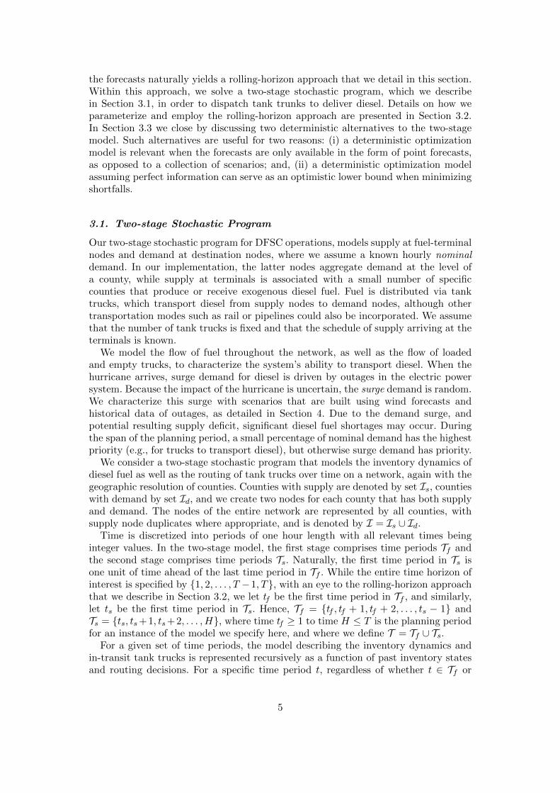
distinguish current decision variables and fixed values from previous time periods, wemodify the latter symbols by adding the modifier “” and include the appropriate timeindex in the formulation. When subscript indices are omitted the term corresponds tothe appropriately dimensioned vector; e.g., Id as a vector of fixed inventories for Idi,t,i ∈ Id, with relevant time periods specified in the formulation.

QTf (Id, Is, r, g, de) =

min∑t∈Tf

[cet (z

e·,t) + cnt (zn·,t)

]+ E[QTs(Id, Is, r, g, de)] (1a)

s.t. Idi,t = Idi,t−1 + b ri,t−1,1 − dni,t − dei,t + zni,t + zei,t ∀i ∈ Id, t ∈ Tf (1b)

Isi,t = Isi,t−1 + si,t − b∑

(j,t′)∈Axi,t

xi,t,j,t′ ∀i ∈ Is, t ∈ Tf (1c)

ri,t−1,1 =∑

(j,t′)∈Ayi,t

yi,t,j,t′ ∀i ∈ Id, t ∈ Tf (1d)

∑(j,t′)∈Ax

i,t

xi,t,j,t′ +∑

(j,t′)∈Ayi,t

yi,t,j,t′ = gi,t−1,1 ∀i ∈ Is, t ∈ Tf (1e)

rj,t,` = rj,t−1,`+1 +∑

i∈Is:(j,t+`)∈Axi,t

xi,t,j,t+`

∀j ∈ Id, t ∈ Tf , ` = 1, 2, . . . , δmax (1f)

gj,t,` = gj,t−1,`+1 +∑

i∈Id:(j,t+`)∈Ayi,t

yi,t,j,t+`

∀j ∈ Is, t ∈ Tf , ` = 1, 2, . . . , δmax (1g)

zni,t ≤ dni,t ∀i ∈ Id, t ∈ Tf (1h)

zei,t ≤ dei,t ∀i ∈ Id, t ∈ Tf (1i)

Idi,tf−1 = Idi,tf−1 ∀i ∈ Id (1j)

Isi,tf−1 = Isi,tf−1 ∀i ∈ Is (1k)

ri,tf−1,1 = ri,tf−1,1 ∀i ∈ Id (1l)

gi,tf−1,1 = gi,tf−1,1 ∀i ∈ Is (1m)

Idi,t ≥ 0 ∀i ∈ Id, t ∈ Tf (1n)

Isi,t ≥ 0 ∀i ∈ Is, t ∈ Tf (1o)

ri,t,l ≥ 0 ∀i ∈ Id, t ∈ Tf , l = 1, 2, . . . , δmax (1p)

gi,t,l ≥ 0 ∀i ∈ Is, t ∈ Tf , l = 1, 2, . . . , δmax (1q)

xi,t,j,t′ ≥ 0, ∀i ∈ Is, t ∈ Tf , (j, t′) ∈ Axi,t (1r)

yi,t,j,t′ ≥ 0, ∀i ∈ Id ∪ Is, t ∈ Tf , (j, t′) ∈ Ayi,t (1s)

zni,t, zei,t ≥ 0 ∀i ∈ Id, t ∈ Tf . (1t)

Here, QTs(·) has identical form as QTf (·) except that: (i) Ts replaces Tf throughoutmodel (1); (ii) ts replaces tf in constraints (1j)-(1m); (iii) the expectation term in (1a)

is eliminated; and (iv) as indicated in QTs(·)’s argument, realizations of deit replace

parameter dei,t in constraints (1b) and (1i).We minimize the sum of penalty costs from nominal and surge shortage and the

expected value of the second stage cost, as shown in the objective function (1a). Con-straints (1b) and (1c) model the inventory of fuel at demand and supply nodes, re-spectively. Constraint (1d) models the balance of trucks at demand nodes by requiring

7

that the number of loaded trucks arriving at a particular node equals the number ofempty trucks leaving from that node at time t. Constraint (1e) follows a similar logicbut for supply nodes, and allows repositioning of an empty tank truck from one supplynode to another and idling at the same supply node. Constraints (1f)–(1g) update thestate variables of loaded and empty trucks according to the number of trucks alreadyin transit and the new departures at time t. Constraints (1h)-(1i) prohibit impropermixing of nominal and surge demands with their shortage variables. Constraints (1j)–(1m) specify boundary conditions, by initializing the state variables inherited from

Id, Is, r, g. Constraints (1n)–(1t) require all variables to be non-negative.

3.2. Rolling-horizon Approach

We embed model (1) in a rolling-horizon approach—see Algorithm 1—over the entiretime span of interest of an arriving hurricane and its aftermath, {1, 2, . . . , T − 1, T}.This set specifies both the hourly temporal resolution and problem horizon. Given this,to define a model instance (1) for the rolling-horizon procedure, we require an initialtime period for decisions, tf , the length of the first stage, F , and the model horizon, H.In this way, Tf = {tf , tf +1, . . . , tf +F −1} and Ts = {tf +F, tf +F +1, . . . , tf +H−1}.

As a practical matter, deploying operational decisions will require advance notice,implying that if the model is proposing decisions that start at time tf , it will useforecasts issued some time before tf , say tf − N . The last element in the rolling-horizon construct is the number of time periods to roll forward, which we denoteR ∈ {1, 2, . . . , F}. This means that the minimum length of time to roll forward is onehour and the maximum is the length of the first-stage set Tf . The following summarizesthe parameters required to run model (1) in our rolling-horizon approach:

• T : problem time horizon• H: model time horizon• F : length of the first stage• R: length of time to roll forward• N : length of time in advance that decisions should be made.

Rolling forward in time essentially means that control variables (x and y in ourmodel) are fixed for all trucks departing at time t ∈ Tf such that tf ≤ t ≤ tf +R− 1.In addition, we assume demand realizations for these time periods are known uponfixing these variables. Of course, these realizations of surge demand will differ from ourforecasts, and hence rolling forward requires updating the actual values of the statevariables, in particular Id. Having fixed the control variables, and having accounted forthe realized surge demand, the new values of the state variables are computed becausethey serve as input to the next instance of model (1), which starts at time tf + R.To formalize this procedure, let TR = {1, R + 1, 2R + 1, . . .} be the set of initial timeperiods at which the model is solved. Algorithm 1 summarizes the procedure describedin this section.

After Algorithm 1 initializes state variables and time-indexed sets for the currentmodel instance, in step 5 we obtain the point forecast of the surge demand for t ∈ Tfand scenarios for surge demand for t ∈ Ts. We discuss this further in the next section.Solving model (1) in step 6 determines the dispatch plan for time periods t ∈ Tr, aset defined in step 7. Re-solving the model in step 10 is simply a convenient way ofcomputing the state variables at the last period in Tr. Step 11 saves this for input tothe next instance of model (1) with the next start time in TR. To understand the way

8

Algorithm 1 Rolling-horizon approach

Require: Id0 , Is0 , r0, g0, initial inventories of fuel and trucks; dn, de, de, nominal and

surge demand.Ensure: void

1: Let Id = Id0 , Is = Is0 , r = r0, g = g0

2: for tf ∈ TR do3: Let Tf = {tf , tf + 1, . . . , tf + F − 1}4: Let Ts = {tf + F, tf + F + 1, . . . , tf +H − 1}5: Retrieve point forecast de and scenarios de issued at time tf −N for Tf and Ts6: Solve model (1) with input (Id, Is, r, g, de) and the scenarios of de

7: Let Tr = {tf , tf + 1, . . . , tf +R− 1} . Start rolling forward8: Fixed control variable x and y for all tank truck departures in t ∈ Tr9: Update surge demand, replacing de with actual realizations for all t ∈ Tr

10: Re-solve model (1) to compute state variables at time to = tf +R− 1

11: Id = Idto , Is = Isto , r = rto , g = gto . End rolling forward12: end for13: return void

in which we roll ahead and fix variables, it is helpful to consider the two extreme casesof R = 1 and R = F . The former only fixes the decisions made in the current initialtime period, tf , and the latter fixes those in all first-stage time periods, i.e., throughperiod tf + F − 1.

3.3. Deterministic Alternative Models

Model (1) is a relatively compact representation of a two-stage stochastic program thatfacilitates different models as special cases. For a model horizon, H, our choice of Fdetermines adaptability to different sample paths. If F = H then the first stage spansthe entire planning horizon, and there is no second stage. Despite losing resolution inthe demand realizations, this model is useful when the only available data come froma single point forecast, and therefore the expectation in (1a) is eliminated. Note alsothat a high-quality point forecast reduces the value of a two-stage model since thescenarios provide little additional information to compute a policy.

The same setup (with F = H) also serves to evaluate ideal cases, not for the purposeof deriving an operations policy, but rather to obtain an optimistic bound on what ispossible. If instead of a point forecast we assume perfect information of future demandthroughout the entire span of the hurricane (problem horizon T ), such a model servesas a benchmark to assess both the two-stage model based on demand scenarios andthe deterministic model based on point forecasts.

4. Case Study: Hurricane Irma

In this section we detail a case study, applying our approach to data available for Hur-ricane Irma, over the period from August 30, 2017 to September 12, 2017. HurricaneIrma caused severe damage in the Caribbean and the State of Florida, although welimit our focus to Florida. We first provide an overview of the DFSC in Florida andof Hurricane Irma. We detail the process of mapping the severity of the hurricane to

9

the demand for diesel fuel in Section 4.1 and of constructing hurricane scenarios fromGEFS data in Section 4.2. In Section 4.3 we describe how the cost function in (1) prior-itizes and penalizes shortfalls in satisfying demand for diesel fuel. With the procedurefor estimating all parameters for the stochastic programming model of Section 3 inplace, we present the computational results and summarize insights in Section 4.5.

Florida does not produce crude oil or have refining capability of significance. Morethan 95% of Florida’s refined petroleum products are transported to the state throughships or pipelines, and there is rarely export of fuel from the state. During HurricaneIrma, because only Florida was hit by the hurricane, the refining capacity of other GulfStates (Texas, Mississippi, Louisiana, and Alabama) was unaffected, and the supplyof diesel fuel quickly resumed after the hurricane. Thus, this case study allows us toisolate the effects of disruption to the demand for diesel relative to the nominal supplychain.

Florida’s daily consumption of refined petroleum products is about 550 thousandbarrels [3], of which diesel is about 27% (150 thousand barrels). We assume that thedemand is approximately equal to the supply because only a small amount of diesel istypically stored in inventory. Among all the end-use sectors for diesel, on-highway use(motor vehicle consumption) makes up around 70% of the demand. Other major usesectors are: vessel bunkering (9%), off-highway (6%, mainly construction use), farming(5%), and commercial (5%) [4]. However, during a hurricane, additional demand arisesto power backup generators for critical infrastructure, while transportation of that fuelmay be interrupted. The typical daily peak electric load for the entire State of Floridais approximately 27.2 GW. We assume that the hurricane can damage a portion ofthe power system, and present the impact of various levels of damage to the DFSC inSection 4.5.

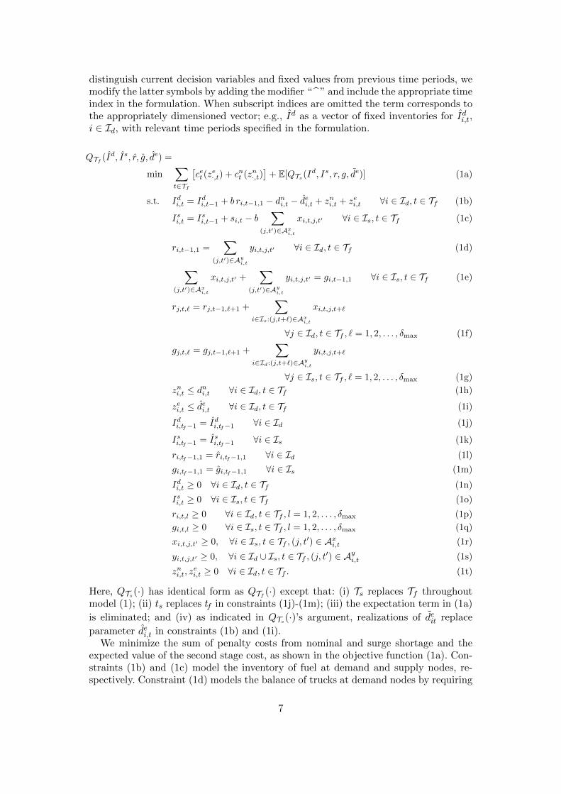
Infrastructure damage during a hurricane is mainly caused by high winds, stormsurge, and inland flooding [55]. Hurricane Irma made landfall as a Category 4 hurri-cane in the Florida Keys on September 10, 2017, and struck southwestern Florida atCategory 3 intensity. The center of Irma passed through the western part of Florida;see Figure 1. According to the NHC [22], peak sustained wind speeds were 115 ktin the Florida Keys and about 100 kt in Southwest Florida, near Marco Island. Themaximum sustained wind recorded inland across South Florida averaged about 60 kt.For portions of the Lower Florida Keys, the storm surge produced inundation levels of5 to 8 ft. As Irma progressed north, the maximum sustained wind speed decreased toabout 55 kt on the east coast and 40 kt on the west, even though the hurricane’s trackwas along the western coast of the state. This contrast is caused by Irma’s large windfield, and similar effects were observed for storm surge: while Irma led to a maximuminundation level of 3-5 ft between Naples and Fort Myers, storm surge flooding of upto 6 ft occurred in Miami-Dade County. In addition, heavy rain was brought to muchof the state by Hurricane Irma, “rainfall totals of 10 to 15 inches were common acrossthe peninsula and the Keys” [22].

4.1. From Weather Data to Diesel Fuel Demand

An important aspect of our analysis is to use data that decision makers can obtain inreal time, as a hurricane approaches. Such resources include hurricane advisories andweather forecasts from the NHC. However, only having weather data is not enoughto estimate the impact of a hurricane. Our analysis, linking the weather forecast dataand the demand for diesel fuel, helps answer the following questions, keeping in mind

10

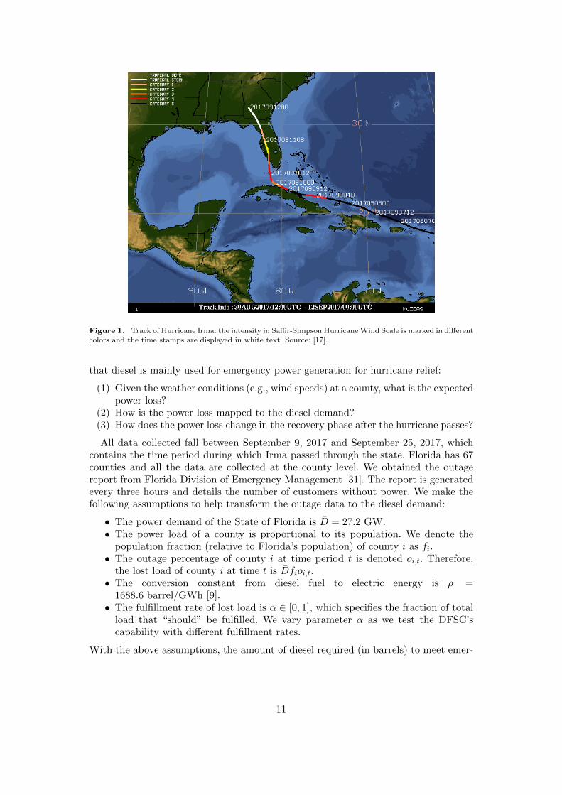
Figure 1. Track of Hurricane Irma: the intensity in Saffir-Simpson Hurricane Wind Scale is marked in different

colors and the time stamps are displayed in white text. Source: [17].

that diesel is mainly used for emergency power generation for hurricane relief:

(1) Given the weather conditions (e.g., wind speeds) at a county, what is the expectedpower loss?

(2) How is the power loss mapped to the diesel demand?(3) How does the power loss change in the recovery phase after the hurricane passes?

All data collected fall between September 9, 2017 and September 25, 2017, whichcontains the time period during which Irma passed through the state. Florida has 67counties and all the data are collected at the county level. We obtained the outagereport from Florida Division of Emergency Management [31]. The report is generatedevery three hours and details the number of customers without power. We make thefollowing assumptions to help transform the outage data to the diesel demand:

• The power demand of the State of Florida is D = 27.2 GW.• The power load of a county is proportional to its population. We denote the

population fraction (relative to Florida’s population) of county i as fi.• The outage percentage of county i at time period t is denoted oi,t. Therefore,

the lost load of county i at time t is Dfioi,t.• The conversion constant from diesel fuel to electric energy is ρ =

1688.6 barrel/GWh [9].• The fulfillment rate of lost load is α ∈ [0, 1], which specifies the fraction of total

load that “should” be fulfilled. We vary parameter α as we test the DFSC’scapability with different fulfillment rates.

With the above assumptions, the amount of diesel required (in barrels) to meet emer-

11

gency generation load in county i within one hour, starting at time t, is:

di,t = αρDfioi,t. (2)

While there is no direct forecast of the outage percentage, oi,t, we can attempt tomap weather conditions to outage levels. We obtain actual weather data from theLocal Climatological Data (LCD) and the weather forecast data from the NationalDigital Forecast Database (NDFD), both maintained by NOAA. LCD data in Floridais collected at 42 locations, each a weather station in a distinct county, usually at anairport, with sustained wind speed, gust speed, pressure, and precipitation recordedhourly. NDFD forecasts are made every three hours at a grid of points for the following168 hours (7 days), and data for the area between the grid points is interpolated byNOAA algorithms. We collect the NDFD data for every county in Florida and the datacontain temperature, sustained wind speed, gust speed, precipitation level, humidity,probability of surface wind speed exceeding 34 kt, 50 kt, and 64 kt.

We also collect storm surge data from the Probabilistic Tropical Storm Surge (P-Surge) model by NOAA, and high water mark (HWM) data from the United StatesGeological Survey (USGS) [66] to estimate storm surge and resulting flooding levels.The P-Surge model estimates the probability that storm surge exceeds a certain heightfor the same grid of points as NDFD data. For a given time, we use the expected stormsurge height at the closest point. HWM data record the height of water marks left byflooding on buildings or trees, which can show the peak flooding level.

For each county we can plot how the outage percentage changed as the hurricaneprogressed, as shown in Figure 2 for Miami-Dade County. From such plots we note:

Observation 1 The outage percentage grows from zero before reaching the peak in asynchronized manner as the wind speed and the storm surge height (not shown)increases;

Observation 2 After its peak, the outage percentage does not appear correlated withthe weather predictors (gust speed, storm surge, etc.);

Observation 3 After the peak, the outage percentage decreases in a roughly linearfashion with the time elapsed since the peak, perhaps due to maintenance efforts.

Based on these observations, we build a quantitative model with two parts: (i) apredictive model to map from the maximum level of a weather condition (e.g., windspeed) to the peak outage percentage; and (ii) a model to estimate the recovery ratefrom the outage.

There has been research about predicting hurricane power outages [e.g., 35, 37,38]. We use a similar statistical analysis approach, but we do not include geographicfeatures such as the land cover and soil variables because our outages are aggregatedby county. Our predictors, in vector x, include the maximum gust speed, the maximumstorm surge height, and the highest recorded water mark height, because damage tothe power system is determined by the worst weather condition; the response variable,y, is the percentage of power outage. We develop a logistic regression model as:

yi =(

1 + e−(β>xi+β0))−1

+ εi, i ∈ I, (3)

where i again indexes counties. Before fitting the regression model, we add one artificialdata point x = 0, y = 0 to represent the absence of a hazard. Our fitted results showthat the storm surge height and the flooding height are not statistically significant—for

12

Figure 2. Power outage percentage (oi,t), LCD gust speed, and NDFD 3-hour forecast gust speed for Miami-

Dade County between September 9, 2017 and September 25, 2017.

Hurricane Irma—even when we add an auxiliary variable indicating coastal counties,which is similar to the result in Guikema et al. [35]. If we keep the maximum gustspeed as the only predictor, we obtain the estimated parameters as β = 0.0889, andβ0 = −6.388. Figure 3 shows that the nonlinear regression model (blue curve) fit tothe data (black dots) across the 67 counties of Florida. For this regression model weobtain R2 = 0.523.

Figure 3. Logistic regression model between the maximum gust speed and the percentage of power loss in

the county.

Power outages decrease during the recovery process after the hurricane passes. Weapproximate the recovery process using a linear function of the elapsed time since the

13

peak outage. Figure 4 plots the peak power loss versus the time to recover to “normaloperations,” defined here as less than 1% outage, across Florida’s 67 counties. Thefitted coefficients of the linear regression model are β = 171.59 and β0 = −7.10,with R2 = 0.6661. The goal is to estimate how long it takes to return to normaloperations so that diesel fuel is no longer needed for emergency generation demand,given the peak level of power outage. For example, the estimated recovery time froman 80% outage is 0.8 × 171.59 − 7.10 = 131.17 hours. In addition, since we assume alinear recovery rate (1.7159 hours to recover 1% of the outage), we can estimate theoutage percentage given the elapsed time since the hurricane peak. In summary, givena time series forecasting gust speeds at county i, wit, t = 1, 2, . . ., and the time indexcorresponding to the maximum gust speed denoted as t, we can estimate the poweroutage rate oi,t using the following:

oi,t =

(

1 + e−(β>wit+β0))−1

t ≤ tβ−1(t− t− β0) t > t.

(4)

Figure 4. Estimated linear relationship between the recovery time and the maximum power outage level.

4.2. Construction of Hurricane Scenarios

With the quantitative models of Section 4.1, given a time series of forecast windspeeds, we can estimate the power outage at corresponding times, and this sectiondescribes how we do so using the GEFS database. GEFS is an ensemble of 21 separateweather forecasting models. A forecast is made every three hours and contains 16 daysof weather information, including the wind gust speed. GFS forecasts are for a grid ofpoints with 1° resolution, with estimates for other points again available by NOAA’sinterpolation e.

We assume equal probabilities for each of these 21 scenarios. When a GEFS forecastis made, we obtain 21 scenarios of wind gust speeds for a county for the next 16 days.

14

Each scenario for these speeds is then mapped to a time series of diesel demand usingequations (2) and (4). Figure 5 illustrates the comparison between the estimated dieseldemand from two GEFS scenarios, the mapped demand from the NDFD gust speedforecasts (available for a shorter horizon), and the diesel demand calculated accordingto actual outage data.

Figure 5. Comparison between the diesel demand profile based on actual outages, the mapped diesel demandfrom two forecast gust speed scenarios, and the mapped diesel demand from NDFD forecast for Miami-Dade

County at 12pm EST September 8th, 2017. Fulfillment rate α = 100%.

4.3. Shortage Cost Setups

An increasing piece-wise linear convex cost function is often used to model conse-quences of growing severity as unsatisfied demand grows (see, e.g., Schutz et al. [62]).We model penalty costs for failing to satisfy nominal demand, cnt , and surge demand,cet , as piece-wise linear convex functions that are parameterized with Kn and Ke pieces,respectively:

cnt (zn·,t) = maxk=1,...,Kn

{ank +mn

k

∑i∈Id

zni,t

}∀t ∈ T (5a)

cet (ze·,t) =

∑i∈Id

[max

k=1,...,Ke

{aek,i +me

k,izei,t

}]∀t ∈ T . (5b)

Here coefficients mek,i, a

ek,i denote the slope and intercept for county-specific surge

shortage while coefficients mnk , a

nk are analogous but for nominal shortage. These func-

tions are incorporated in model (1) by adding auxiliary variables and constraints akinto the right-hand side of constraints (5a) and (5b). Our choice for the penalty functionsis motivated by the fact that the effects of nominal and surge shortages at differentlevels. Because trucks run on diesel fuel, if the total nominal shortage is too high,we do not have enough diesel fuel to dispatch trucks and the transportation networkcannot function. Therefore, in equation (5a), the nominal shortage cost is calculatedin terms of the aggregated nominal shortage across the DFSC. On the other hand,

15

surge shortage cost described in equation (5b) is calculated at each county due to thecost of not powering local facilities.

While we distinguish nominal and surge demand in global and local ways, as justdescribed, our piece-wise linear functions have a total of four pieces and slopes withKe = Kn = 2, ordered in decreasing steepness: (i) nominal demand, 90-100%; (ii) surgedemand, 50%-100%; (iii) surge demand, 0%-50%; and (iv) nominal demand, 0-90%.Thus the most important demand to satisfy is global nominal demand, until “only”90% remains unmet. Then, we should satisfy surge demand in each county until 50%remains unmet, and then again until surge demand is fully satisfied. The remainingfuel is then used to satisfy nominal demand. We assume 10% of the nominal demandis needed for key transportation across the state, including for tank trucks, and this iswhy the first piece of the nominal demand has the steepest shortfall cost. After that,we prioritize surge demand at critical infrastructure such as hospitals, municipal watersystems, and facilities for first responders. Therefore, we set a high penalty cost forthe surge shortage, with two levels of priority. Table 4 summarizes the values for ank ,mnk , aek,i, and me

k,i for a given time period t.

Piece kSurge Nominal

mek,i aek,i mn

k ank1 2 0 1 0

2 5 (me2,i −me

1,i) · 0.5 · dei,t 10 (mn2 −mn

1 ) · 0.9 ·∑

i∈Id dni,t

Table 4. Parameters used to define penalty functions for failing to satisfy demand for diesel fuel. See equa-

tion (5) and model (1).

4.4. Solution Stability

Model (1) can have multiple optimal solutions, particularly in the early part of theplanning period, because multiple dispatch plans achieve zero shortage before the hur-ricane arrives and demand surges. Under the rolling-horizon approach, small changesin the solution in early time periods can lead to differences as large as 5% in theexpected shortage cost as we replicate experiments. To obtain a stable solution, weincorporate a tie-breaking mechanism by small adjustments in the objective function:

• for variables Idi,t, we use a per-barrel reward for inventory of fuel at demand sites

with a coefficient of −(1.001)tfi|Tf |−1;• for variables x and y, we use a penalty of 10−4 · τij to discourage long-distance

transport, where τij is the travel time i from j embedded in sets Ax and Ay.

Adding these tie-breaking coefficients does not degrade the total penalty cost formodels with a long horizon, but helps significantly in stabilizing solutions in the rolling-horizon procedure. We employ these objective function terms in all experiments in thefollowing section.

4.5. Experimental Results

We present experimental results of our DFSC optimization model in this section. Wecompare shortfall penalties for surge and nominal demand obtained by running Algo-rithm 1 with the stochastic programming model (1), using deterministic alternativesas benchmarks, as described in Section 3.3. We also test our model with controlled

16

parameters, H,F,R,N and α (see Sections 3.2 and 4.1) in order to evaluate their ef-fect on the model and obtain operational insights. All results that we report use eithera point forecast or a set of scenarios to dispatch tank trucks, but use actual poweroutages from Irma, and the associated demand for diesel, to compute shortages.

We use a single thread on a 2.4 GHz Intel Xeon core with 8 GB of RAM to runall tests. All models are constructed using the Gurobi Python API and solved byGurobi 8.1.1 [36] with default parameters. For all tests, solving both the optimizationproblem (1) and all deterministic alternatives takes less than one hour, which is theunit time period. Thus, the computational performance does not affect the executionof the rolling-horizon approach, and so we focus our presentation on the value ofour model and analysis of model parameters, rather than the required computationaleffort.

4.5.1. Comparison with Deterministic Benchmarks

We compare three deterministic alternatives to our stochastic program (denoted“GEFS”), to examine the value of modeling uncertainty and how much improvementcan be made under a perfect hurricane forecast. As described in Section 3.3, as analternative we can run Algorithm 1 with deterministic demand profiles instead of 21scenarios. The ways of doing so are via NDFD, average GEFS (denoted “GAVG”),and perfect information (denoted “PI”). For NDFD, we use the point forecast for windgust speed from NDFD as the deterministic forecast; for GAVG, we use the mean of21 scenarios; for PI, we use the actual demand data, i.e., based on actual outages. Inaddition, we solve a deterministic optimization problem with demand information forthe entire problem horizon T , denoted “BEST.” While PI essentially provides a bench-mark on best practice, given a set of H,F,R and N , BEST gives the best achievablepractice with the distinction being that PI can only see to the model horizon H whileBEST has access to perfect information to the problem horizon T .

Figure 6 shows surge and nominal shortages and the total demand across time.These results assume α = 0.5 of the demand must be satisfied and uses rolling-horizonparameters of H = 96, F = 72, R = 24 and N = 24 hours. The colored lines specifyshortages for the four alternatives, and the black line indicates total demand, account-ing for α. The cumulative shortage and penalty results at the end of the problem timehorizon are summarized in Table 5.

AlternativeSurge Nominal Total Surge Nominal Total

Shortage Shortage Shortage Penalty Penalty PenaltyGEFS 161.4 1012.4 1173.8 370,309.9 1,012,352.2 1,382,662.0NDFD 469.0 705.3 1174.3 1,227,241.5 705,335.0 1,932,576.5GAVG 204.2 969.6 1173.8 489,425.8 969,608.0 1,459,033.8PI 1.9 1171.6 1173.5 3825.1 1,171,584.0 1,175,409.1BEST 0.0 1173.5 1173.5 0.0 1,173,496.6 1,173,496.6

Table 5. Cumulative surge, nominal and total shortages and their penalties at the end of time horizon for

different alternatives, with parameters α = 0.5 and H = 96, F = 72, R = 24 and N = 24 hours. The unit fordemand data is thousand of barrels.

If more diesel is delivered to a county than its demand, it goes unused, but mostdiesel is consumed. Thus we observe from Figure 6 and Table 5 that the total shortagesfor different alternatives are similar. The table and figure show that the alternativesdiffer in their treatment of surge demand and nominal demand. Given the cost struc-ture in Section 4.3, after satisfying the first 10% of nominal demand, surge demandshould be prioritized over nominal demand.

17

PI yields a total penalty cost 0.1% higher than BEST as PI makes decisions lookingonly 96 hours into the future. Together PI and BEST achieve the lowest penalty costsby incurring larger nominal shortages early in the time horizon so that accumulatedinventory is better used when the hurricane arrives. This suggests that knowing thedemand ahead of time can save at least 15% of costs compared to the next bestalternative, GEFS.

Putting aside a perfect weather forecast, GEFS performs better than GAVG andNDFD, which shows the value of incorporating multiple scenarios. GEFS achieves161.4 thousand barrels of surge shortage and a total cost of about 1.38 × 106, whichis 28.5% and 5.2% lower than respective total costs of NDFD and GAVG. Thus, thereis value in hedging against multiple possible hurricane paths.

AlternativeSurge Nominal Total Surge Nominal Total

Shortage Shortage Shortage Penalty Penalty PenaltyGEFS 142.7 1031.0 1173.8 312,191.3 1,031,032.5 1,343,223.9NDFD 575.2 599.1 1174.2 1,675,772.6 599,072.6 2,274,845.3GAVG 157.9 1015.9 1173.8 356,436.9 1,015,872.9 1,372,309.8PI 0.0 1173.5 1173.5 0.0 1,173,496.6 1,173,496.6

Table 6. Cumulative surge, nominal and total shortages and their penalties at the end of time horizon for

different alternatives, with parameters α = 0.5 and H = 96, F = 72, R = 12 and N = 12 hours. The unit for

demand data is thousand of barrels.

We repeat the same analysis for the same horizon (H = 96) and first-stage length(F = 72), but a shorter rolling period (R = 12) and a shorter span to make decisions inadvance (N = 12), with results in Table 6 and Figure 7. With more frequent updatesof our decisions, and more up-to-date forecasts, GEFS, GAVG, and PI all improve overthe results of Table 5 while NDFD degrades, surprisingly. What is consistent is thatNDFD’s results are inferior to those of GAVG and GEFS. These two test instancesare also consistent with the general trend of relative costs of these alternatives:

PI < GEFS < GAVG < NDFD.

The combination of the shorter rolling period and more up-to-date forecasts trans-lates into a more informed and adaptive response. The model with perfect informationreduces the surge shortage to zero, and GEFS and GAVG decrease surge shortage.Comparing the two figures, we see that the nominal shortage curve shifts to the leftand the surge shortage is lower in Figure 7, as the optimization starts moving fuelfor nominal demand earlier to accumulate inventory in preparation for the upcomingsurge demand. For NDFD, this increased adaptability does not translate to a decreasedsurge shortage or a decreased total cost, potentially because the NDFD forecast is sig-nificantly more variable than GEFS over time.

4.5.2. Analysis of Model Parameters

The above comparison between two tests with different R and N motivates us toexplore how different parameters affect performance. We run multiple tests, with de-viations from the base case of H = 96, F = 24, R = 24, N = 24, α = 0.5 to examinethe impact of each of H,F,R,N and α on the shortage and the penalty cost.

Table 7 shows the results of the parametric tests, with the results split into sixgroups. The first group shows that an increased first-stage length decreases the surgeshortage and total cost up to a limit, i.e., some stochastic hedging brings value. Thesecond and third sets of results show value in simultaneously increasing the model

18

(H,F ,R,N ,α)Surge Nominal Total Surge Nominal Total

Shortage Shortage Shortage Penalty Penalty Penalty(96,24,24,24,0.5) 197.8 976.0 1173.8 459,564.7 975,999.3 1,435,564.0(96,48,24,24,0.5) 172.7 1001.1 1173.8 391,341.4 1,001,080.2 1,392,421.6(96,72,24,24,0.5) 161.4 1012.4 1173.8 370,309.9 1,012,352.2 1,382,662.0(96,96,24,24,0.5) 204.2 969.6 1173.8 489,425.8 969,608.0 1,459,033.8(96,24,24,24,0.5) 197.8 976.0 1173.8 459,564.7 975,999.3 1,435,564.0(120,48,24,24,0.5) 158.4 1015.4 1173.8 363,113.7 1,015,368.6 1,378,482.3(144,72,24,24,0.5) 153.3 1020.5 1173.8 347,197.0 1,020,467.1 1,367,664.1(96,24,24,24,0.5) 197.8 976.0 1173.8 459,564.7 975,999.3 1,435,564.0(72,24,24,24,0.5) 201.7 972.1 1173.8 470,461.3 972,090.6 1,442,552.0(48,24,24,24,0.5) 328.3 845.5 1173.8 751,868.0 845,507.9 1,597,375.9(96,24,24,24,0.5) 197.8 976.0 1173.8 459,564.7 975,999.3 1,435,564.0(96,24,12,24,0.5) 176.4 997.3 1173.6 390,568.3 997,265.8 1,387,834.2(96,24,6,24,0.5) 159.4 1014.2 1173.7 341,405.3 1,014,229.9 1,355,635.2(96,24,24,24,0.5) 197.8 976.0 1173.8 459,564.7 975,999.3 1,435,564.0(96,24,24,12,0.5) 201.5 972.4 1173.9 421,761.8 972,370.9 1,394,132.7(96,24,24,6,0.5) 142.6 1030.9 1173.5 316,316.1 1,030,869.4 1,347,185.5(96,24,24,24,1.0) 1112.0 1280.2 2392.2 2,626,870.5 1,280,238.1 3,907,108.7(96,24,24,24,0.5) 197.8 976.0 1173.8 459,564.7 975,999.3 1,435,564.0(96,24,24,24,0.2) 20.4 422.3 442.7 45,723.6 422,341.4 468,065.0

Table 7. Cumulative surge, nominal and total shortages and their penalties at the end of time horizon for

different sets of parameters, with parameters α = 0.5, H = 96, F = 72, R = 24 and N = 24 serving as the basecase. The unit for demand data is thousand of barrels.

horizon H and the length of the first stage F . The fourth and fifth sets suggest thatas we shorten the time periods to roll forward, R, or the delay in the forecast, N ,the total cost and the surge shortage decreases, because it allows more flexible andadaptive planning. These quantify the value of pursuing a more flexible and quick-responsive operation.

Finally, we inspect how the shortage and total cost are affected by different fulfill-ment rates. When the supply is fixed, an increased fulfillment rate increases demandand leads to larger shortages and higher costs. However, the relationship is not lin-ear in that the surge shortage, total shortage, and shortage costs grow more quicklyas the fulfillment rate grows. This suggests that it is key to prioritize critical loadsand that there would be benefits to local self-reliance either by reducing loads or viastorm-resilient microgrids.

5. Conclusions

In this paper, we formulated and solved a model for diesel fuel supply chain opera-tions under a disruption caused by a hurricane. It is key to be proactive in planningbefore the hurricane arrives, accounting for its uncertain path and intensity. We uti-lized weather forecasts from NOAA to construct hurricane scenarios and mapped theweather data to demand for diesel fuel, which is mainly used in emergency power gen-eration and transportation of fuel. We proposed a rolling-horizon approach: at eachdecision point, we solved a two-stage stochastic program with the GEFS-informedhurricane scenarios, committed to the dispatch of tank trucks until the next time adecision is made, and a new stochastic program was solved with updated scenarios.

We created a case study for Hurricane Irma, considering realistic settings in model-ing diesel demand from accessible public data. Computational results justify the value

19

of our stochastic programming model, and sensitivity analysis on model parametersprovide useful insights about valuable improvements for preparedness.

In the context of Hurricane Irma, only wind speed was predictive of power outages,but more generally we expect further weather predictors, such as rainfall and stormsurge, to add predictive value. Our rolling-horizon approach can be extended to amulti-stage stochastic program, which poses more challenging issues in how to con-struct a reasonable model that can be decomposed and solved efficiently. Moreover, itis important to coordinate the DFSC and other infrastructure networks for hurricanerelief. In the future, we aim to augment our model, and rolling-horizon algorithm,with interfaces to port operations [27], transportation networks [50], and electricitynetworks [72] to better inform decision support for hurricane response and relief.

Acknowledgments

This work was supported by the U.S. Department of Homeland Security under GrantAward 2017-ST-061-QA0001. The views and conclusions contained in this documentare those of the authors and should not be interpreted as necessarily representing theofficial policies, either expressed or implied, of the U.S. Department of Homeland Se-curity. We thank the Center for Nonlinear Studies at Los Alamos National Laboratoryfor partially supporting Haoxiang Yang’s work. The authors thank Lauren Davis, PituMirchandani, and Giulia Pedrielli for multiple conversations that contributed to ourwork. And, the authors thanks Craig S. Gordon, Laura Laybourn, and Eric Rollisonfor suggestions that helped frame the analysis.

References

[1] Is your water or wastewater system prepared? What you need to know about generators.Technical Report EPA 901-F-09-027, United States Environmental Protection AgencyNew England, September 2009.

[2] Power resilience: Guide for water and wastewater utilities. Technical Report EPA800–R–15–004, United States Environmental Protection Agency, December 2015.

[3] Hurricane Irma: Infrastructure impact assessment: Florida refined petroleum productavailability 1130 EDT September 8, 2017. Technical report, National Protection andPrograms Directorate, Office of Cyber and Infrastructure Analysis, September 2017.

[4] Florida sales of distillate fuel oil by end use, December 2017. URL https://www.eia.

gov/dnav/pet/pet_cons_821dst_dcu_SFL_a.htm.[5] The 2017 Florida statutes, Title XXXIII, Chapter 526, March 2018. URL

http://www.leg.state.fl.us/statutes/index.cfm?App_mode=Display_Statute&

URL=0500-0599/0526/Sections/0526.143.html.[6] Role of diesel generators in the healthcare industry, 2018. URL http://www.

dieselserviceandsupply.com/Generators_Healthcare.aspx. Accessed: 2018-03-05.[7] Diesel generators provide power in critical times, March 2018. URL http://www.

dieselserviceandsupply.com/Hurricanes_Backup_Power.aspx. Accessed: 2018-03-05.

[8] Hurricane Irma’s effect on Florida’s fuel distribution system and recommended im-provements. Technical report, The Florida Department of Transportation, January2018. URL http://www.fdot.gov/info/CO/news/newsreleases/020118_FDOT-Fuel-

Report.pdf.[9] Approximate diesel fuel consumption chart, 2019. URL https://www.

20

dieselserviceandsupply.com/temp/Fuel_Consumption_Chart.pdf. Accessed:2019-08-21.

[10] C. Abbey, D. Cornforth, N. Hatziargyriou, K. Hirose, A. Kwasinski, E. Kyriakides,G. Platt, L. Reyes, and S. Suryanarayanan. Powering through the storm: microgridsoperation for more efficient disaster recovery. IEEE Power and Energy Magazine, 12(3):67–76, 2014.

[11] A. Adhitya, R. Srinivasan, and I. A. Karimi. Heuristic rescheduling of crude oil operationsto manage abnormal supply chain events. AIChE Journal, 53(2):397–422, 2007.

[12] A. M. Afshar and A. Haghani. Heuristic framework for optimizing hurricane evacuationoperations. Transportation Research Record, 2089(1):9–17, 2008.

[13] D. Alem, A. Clark, and A. Moreno. Stochastic network models for logistics planning indisaster relief. European Journal of Operational Research, 255(1):187–206, 2016.

[14] G. Alfke, W. W. Irion, and O. S. Neuwirth. Oil refining. Ullmann’s Encyclopedia ofIndustrial Chemistry, 2007.

[15] N. Altay and W. G. Green. OR/MS research in disaster operations management. EuropeanJournal of Operational Research, 175(1):475–493, 2006.

[16] J. S. Aronofsky and A. C. Williams. The use of linear programming and mathematicalmodels in under-ground oil production. Management Science, 8(4):394–407, 1962.

[17] Scott Bachmeier. Hurricane Irma storm-track. http://tropic.ssec.wisc.edu/storm_

archive/2017/storms/11L/11L.html, 2017. Accessed: 2019-08-18.[18] F. Bajak and R. Dunklin. Explosions rock flood-crippled chemical plant near Houston,

Sptember 2017. URL https://apnews.com/43288ccafa394ae59fd8a548b23a29a1.[19] J. D. Bales. Effects of Hurricane Floyd inland flooding, September–October 1999, on

tributaries to Pamlico Sound, North Carolina. Estuaries, 26(5):1319–1328, Oct 2003.[20] A. Beheshtian, K. P. Donaghy, R. R. Geddes, and O. M. Rouhani. Planning resilient

motor-fuel supply chain. International Journal of Disaster Risk Reduction, 24:312–325,2017.

[21] B. Blanton, K. Dresback, B. Colle, R. Kolar, R. Vergara, Y. Hong, N. Leonardo, R. A.Davidson, L. K. Nozick, and T. Wachtendorf. An integrated scenario ensemble-basedframework for hurricane evacuation modeling: Part 2—hazard modeling. Risk Analysis,40(1):117–133, 2020.

[22] J. P. Cangialosi, A. S. Latto, and R. Berg. National Hurricane Center tropical cyclonereport: Hurricane Irma. Research report AL112017, National Hurricane Center, 2018.URL https://www.nhc.noaa.gov/data/tcr/AL112017_Irma.pdf.

[23] A. Charnes, W. W. Cooper, and B. Mellon. Blending aviation gasolines–a study inprogramming interdependent activities in an integrated oil company. Econometrica, 20(2):135–159, 1952.

[24] A. Charnes, W. W. Cooper, and B. Mellon. A model for programming and sensitivityanalysis in an integrated oil company. Econometrica, 22(2):193–217, 1954.

[25] D. Cullen. Fuel market impact of Hurricanes Harvey & Irma, September2017. URL http://www.breakthroughfuel.com/blog/fuel-market-impact-of-

hurricanes-harvey-irma-advisor-pulse/.[26] R. A. Davidson, L. K. Nozick, T. Wachtendorf, B. Blanton, B. Colle, R. L. Kolar, S. DeY-

oung, K. M. Dresback, W. Yi, K. Yang, and N. Leonardo. An integrated scenarioensemble-based framework for hurricane evacuation modeling: Part 1—decision supportsystem. Risk Analysis, 40(1):97–116, 2020.

[27] L. B. Davis and D. Edwards. Determining optimal fuel strategies under uncertainty.Research report, North Carolina A&T State University, 2020.

[28] L. B. Davis, F. Samanlioglu, X. Qu, and S. Root. Inventory planning and coordinationin disaster relief efforts. International Journal of Production Economics, 141(2):561–573,2013.

[29] M. A. H. Dempster, N. H. Pedron, E. A. Medova, J. E. Scott, and A. Sembos. Planninglogistics operations in the oil industry. Journal of the Operational Research Society, 51(11):1271–1288, 2000.

21

[30] L. F. Escudero, F. J. Quintana, and J. Salmeron. CORO, a modeling and an algorithmicframework for oil supply, transformation and distribution optimization under uncertainty.European Journal of Operational Research, 114(3):638–656, 1999.

[31] Florida Division of Emergency Management. Hurricane Irma: Power outage data, Septem-ber 2017. URL http://floridadisaster.org/info/outage_reports/irma/.

[32] European Centre for Medium-Range Weather Forecasts. Modelling and prediction, March2019. URL https://www.ecmwf.int/en/research/modelling-and-prediction.

[33] Global Climate and Weather Modeling Branch. The GFS atmospheric model. Tech-nical report, National Weather Service, 2003. URL https://www.emc.ncep.noaa.gov/

officenotes/newernotes/on442.pdf.[34] A. D. Gonzalez, L. Duenas Osorio, M. Sanchez-Silva, and A. Medaglia. The interdepen-

dent network design problem for optimal infrastructure system restoration. Computer-Aided Civil and Infrastructure Engineering, 31(5):334–350, 2016.

[35] S. D. Guikema, R. Nateghi, S. M. Quiring, A. Staid, A. C. Reilly, and M. Gao. Predictinghurricane power outages to support storm response planning. IEEE Access, 2:1364–1373,2014.

[36] Gurobi Optimization, Inc. Gurobi Optimizer Reference Manual, 2016. URL http://www.

gurobi.com.[37] S. R. Han, S. D. Guikema, and S. M. Quiring. Improving the predictive accuracy of

hurricane power outage forecasts using generalized additive models. Risk Analysis: AnInternational Journal, 29(10):1443–1453, 2009.

[38] S. R. Han, S. D. Guikema, S. M. Quiring, K. H. Lee, D. Rosowsky, and R. A. Davidson.Estimating the spatial distribution of power outages during hurricanes in the Gulf Coastregion. Reliability Engineering & System Safety, 94(2):199–210, 2009.

[39] M. L. Itria, M. Kocsis-Magyar, A. Ceccarelli, P. Lollini, G. Giunta, and A. Bondavalli.Identification of critical situations via event processing and event trust analysis. Knowl-edge and Information Systems, 52(1):147–178, 2017.

[40] A. Kwasinski. Hurricane Sandy effects on communication systems. Technical ReportPR-AK-0112-2012, The University of Texas at Austin, 2012.

[41] A. Kwasinski. Lessons from field damage assessments about communication networkspower supply and infrastructure performance during natural disasters with a focus onHurricane Sandy. In FCC Workshop on Network Resiliency, 2013.

[42] D. R. Levinson. Hospital emergency preparedness and response during superstorm Sandy.Technical Report OEI-06-13-00260, Department of Health and Human Services, 2014.

[43] X. Li, R. Batta, and C. Kwon. Effective and equitable supply of gasoline to impactedareas in the aftermath of a natural disaster. Socio-Economic Planning Sciences, 57:25–34,2017.

[44] C. Lima, S. Relvas, and A. P. F. D. Barbosa-Povoa. Downstream oil supply chain man-agement: a critical review and future directions. Computers & Chemical Engineering, 92:78–92, 2016.

[45] E. J. Lodree and S. Taskin. Supply chain planning for hurricane response with wind speedinformation updates. Computers & Operations Research, 36(1):2–15, 2009.

[46] E. J. Lodree and S. Taskin. A Bayesian decision model with hurricane forecast updates foremergency supplies inventory management. Journal of the Operational Research Society,62(6):1098–1108, 2011.

[47] N. Lorenzi. Critical features of emergency power generators, September 2015. URLhttps://www.hfmmagazine.com/articles/1712-critical-features-of-emergency-

power-generators.[48] R. A. Luettich, J. J. Westerink Jr., and N. W. Scheffner. ADCIRC: an advanced three-

dimensional circulation model for shelves coasts and estuaries, report 1: theory andmethodology of ADCIRC-2DDI and ADCIRC-3DL. Technical Report DRP-92-6, U.S.Army Engineers Waterways Experiment Station, 1992.

[49] M. Meraklı and S. Kucukyavuz. Risk aversion to parameter uncertainty in markov decisionprocesses with an application to slow-onset disaster relief. IISE Transactions, pages 1–21,

22

2019. URL https://doi.org/10.1080/24725854.2019.1674464.[50] P. Mirchandani and K. G. Ayu. A data-driven probabilistic simulation model and visu-

alization for hurricane. Research report, Arizona State University, 2020.[51] National Hurricane Center. Hurricane preparedness: Hazards, July 2019. URL https:

//www.nhc.noaa.gov/prepare/hazards.php.[52] National Hurricane Center. NHC track and intensity models, March 2019. URL https:

//www.nhc.noaa.gov/modelsummary.shtml.[53] S. M. S. Neiro and J. M. Pinto. A general modeling framework for the operational planning

of petroleum supply chains. Computers & Chemical Engineering, 28(6-7):871–896, 2004.[54] N. Noyan. Risk-averse two-stage stochastic programming with an application to disaster

management. Computers & Operations Research, 39(3):541–559, 2012.[55] U.S. Department of Homeland Security. Foundational methodology to support infras-

tructure decision analysis: Initial development efforts and test case. Research report, U.S.Department of Homeland Security, 2009.

[56] Met Office. Met Office numerical weather prediction models, March 2019. URLhttps://www.metoffice.gov.uk/research/modelling-systems/unified-model/

weather-forecasting.[57] G. G. Pacheco and R. Batta. Forecast-driven model for prepositioning supplies in prepa-

ration for a foreseen hurricane. Journal of the Operational Research Society, 67:98–131,2016.

[58] T. Powell, D. Hanfling, and L. O. Gostin. Emergency preparedness and public health:the lessons of Hurricane Sandy. Journal of the American Medical Association, 308(24):2569–2570, 2012.

[59] C. G. Rawls and M. A. Turquist. Pre-positioning of emergency supplies for disasterresponse. Transportation Research Part B: Methodological, 44:521–534, 2010.

[60] M. Rezaei-Malek, R. Tavakkoli-Moghaddam, B. Zahiri, and A. Bozorgi-Amiri. An inter-active approach for designing a robust disaster relief logistics network with perishablecommodities. Computers & Industrial Engineering, 94:201–215, 2016.

[61] I. N. Robertson, H. R. Riggs, S. C. Yim, and Y. L. Young. Lessons from HurricaneKatrina storm surge on bridges and buildings. Journal of Waterway, Port, Coastal, andOcean Engineering, 133(6):463–483, 2007.

[62] P. Schutz, L. Stougie, and A. Tomasgard. Stochastic facility location with general long-runcosts and convex short-run costs. Computers and Operations Research, 35(9):2988–3000,2008.

[63] T. N. Sear. Logistics planning in the downstream oil industry. Journal of the OperationalResearch Society, 44(1):9–17, 1993.

[64] W. C. Skamarock, J. B. Klemp, J. Dudhia, D. O. Gill, D. M. Barker, W. Wang, andJ. G. Powers. A description of the advanced research wrf version 2. Technical ReportNCAR/TN-468+ STR, National Center For Atmospheric Research, 2005.

[65] Y. Suzuki. Disaster-relief logistics with limited fuel supply. Journal of Business Logistics,33(2):145–157, 2012.

[66] The United States Geological Survey. USGS flood event viewer: providing hurricaneand flood response data, September 2017. URL https://stn.wim.usgs.gov/fev/

#IrmaSeptember2017.[67] P. J. Vickery, J. Lin, P. F. Skerlj, L. A. Twisdale, and K. Huang. HAZUS-MH hurricane

model methodology. I: hurricane hazard, terrain, and wind load modeling. Natural HazardsReview, 7(2):82–93, 2006.

[68] J. Wang, Y. Hong, L. Li, J. J. Gourley, S. Khan, K. K. Yilmaz, R. F. Adler, F. S. Policelli,S. Habib, D. Irwn, A. S. Limaye, T. Korme, and L. Okello. The coupled routing and excessstorage (CREST) distributed hydrological model. Hydrological Sciences Journal, 56(1):84–98, 2011.

[69] M. J. Widener and M. W. Horner. A hierarchical approach to modeling hurricane disasterrelief goods distribution. Journal of Transport Geography, 19(4):821–828, 2011.

[70] K. Yagci Sokat, R. Zhou, I. S. Dolinskaya, K. Smilowitz, and J. Chan. Capturing real-time

23

data in disaster response logistics. Journal of Operations and Supply Chain Management,9(1):23–54, 2016.

[71] K. Yagci Sokat, I. S. Dolinskaya, K. Smilowitz, and R. Bank. Incomplete informationimputation in limited data environments with application to disaster response. EuropeanJournal of Operational Research, 269(2):466–485, 2018.

[72] H. Yang and H. Nagarajan. Optimal power flow in distribution networks under stochasticN-1 disruptions. In 2020 Power Systems Computation Conference (PSCC) Proceedings,2020.

24

Figure 6. Surge (top), nominal (middle), and total (bottom) demands are shown in black. Unmet demand

under the stochastic program (GEFS), two deterministic models (GAVG and NDFD) as well as under perfectinformation (PI) are also shown. All values are in barrels of diesel fuel for parameters α = 0.5 and H = 96, F =

72, R = 24 and N = 24 hours.

25

Figure 7. This figure follows the same format as Figure 6 except that Algorithm 1 now uses parametersα = 0.5 and H = 96, F = 72, R = 12 and N = 12 hours. Decreasing R and N tends to increase the nimbleness

of the strategy.

26