Optimization WS 2017/18 Lecturer { Dan Rust, Tutor { Mima ...
48
Optimization, WS 2017/18 Lecturer – Dan Rust, Tutor – Mima Stanojkovski Part 1. Convergence in Metric Spaces (about 7 Lectures) Supporting Literature: Angel de la Fuente, “Mathematical Methods and Models for Economists”, Chapter 2 Contents 1 Convergence in Metric Spaces 1 1.1 Definition of Metric and Normed Spaces ................... 2 1.2 Sequences and Convergence .......................... 9 1.3 Open and Closed Sets ............................. 12 1.4 Limits of Functions, Continuity ........................ 14 1.5 Cauchy Sequences, Complete Metric Spaces ................. 18 1.6 Banach Contraction Mapping Theorem .................... 18 1.7 Cantor Intersection Theorem .......................... 22 1.8 Separable Spaces ................................ 23 1.9 Basic Examples revisited ............................ 24 1.10 Linear Mappings (Operators) in Normed Spaces ............... 28 1.11 Compact Sets (Heine-Borel, Bolzano-Weierstrass) .............. 31 1.12 Continuous Functions on Compact Sets .................... 36 1.13 Equivalent Metrics and Norms ......................... 39 1.14 Back to the Reals: R d as a Banach Space ................... 42 1.15 Summary: Structures on Vector Spaces .................... 44 1.16 Multivalued Mappings (Correspondences) ................... 46 1 Convergence in Metric Spaces Acknowledgements These Lecture notes were kindly provided by Dr. Tanja Pasurek. They were edited by Dr. Dan Rust and Chrizaldy Neil Manibo. 1
Transcript of Optimization WS 2017/18 Lecturer { Dan Rust, Tutor { Mima ...

Optimization, WS 2017/18
Lecturer – Dan Rust, Tutor – Mima Stanojkovski
Part 1. Convergence in Metric Spaces
(about 7 Lectures)
Supporting Literature: Angel de la Fuente, “Mathematical Methods and Models
for Economists”, Chapter 2
Contents
1 Convergence in Metric Spaces 1
1.1 Definition of Metric and Normed Spaces . . . . . . . . . . . . . . . . . . . 2
1.2 Sequences and Convergence . . . . . . . . . . . . . . . . . . . . . . . . . . 9
1.3 Open and Closed Sets . . . . . . . . . . . . . . . . . . . . . . . . . . . . . 12
1.4 Limits of Functions, Continuity . . . . . . . . . . . . . . . . . . . . . . . . 14
1.5 Cauchy Sequences, Complete Metric Spaces . . . . . . . . . . . . . . . . . 18
1.6 Banach Contraction Mapping Theorem . . . . . . . . . . . . . . . . . . . . 18
1.7 Cantor Intersection Theorem . . . . . . . . . . . . . . . . . . . . . . . . . . 22
1.8 Separable Spaces . . . . . . . . . . . . . . . . . . . . . . . . . . . . . . . . 23
1.9 Basic Examples revisited . . . . . . . . . . . . . . . . . . . . . . . . . . . . 24
1.10 Linear Mappings (Operators) in Normed Spaces . . . . . . . . . . . . . . . 28
1.11 Compact Sets (Heine-Borel, Bolzano-Weierstrass) . . . . . . . . . . . . . . 31
1.12 Continuous Functions on Compact Sets . . . . . . . . . . . . . . . . . . . . 36
1.13 Equivalent Metrics and Norms . . . . . . . . . . . . . . . . . . . . . . . . . 39
1.14 Back to the Reals: Rd as a Banach Space . . . . . . . . . . . . . . . . . . . 42
1.15 Summary: Structures on Vector Spaces . . . . . . . . . . . . . . . . . . . . 44
1.16 Multivalued Mappings (Correspondences) . . . . . . . . . . . . . . . . . . . 46
1 Convergence in Metric Spaces
Acknowledgements These Lecture notes were kindly provided by Dr. Tanja Pasurek.
They were edited by Dr. Dan Rust and Chrizaldy Neil Manibo.
1

1.1 Definition of Metric and Normed Spaces
Of fundamental importance in mathematical analysis is the notion of limit and convergence
(e.g., for real numbers, complex numbers, vectors in Rn, functions etc.). This constitutes a
basis for defining two fundamental operations: differentiation and integration of functions.
The notion of limit involves a possibility to measure a “distance” between the objects.
Extending the well-known notion of the Euclidean distance
d(x, y) := |x− y| between two reals x, y ∈ R, or
d(x, y) := ‖x − y‖ =√
(x1 − y1)2 + (x2 − y2)2 + (x3 − y3)2 between two points x :=
(x1, x2, x3), y := (y1, y2, y3) ∈ R3,
we naturally come to the notion of metric space, which is the basic one in modern math-
ematics. Roughly speaking, a metric space is a set in which we have defined a distance,
i.e., a metric. Introducing the metric, we can study the properties of limits independently
on the concrete nature of objects under consideration.
History: The notion of a metric space was first introduced by the French mathemati-
cian M. Frechet (1906). This area of mathematics is now seen as a part of Functional
Analysis (FA).
Functional Analysis (as a branch of Mathematical Analysis) studies vector space (in
general, infinite-dimensional) endowed with some kind of limit-related structure (e.g. inner
product, norm, metric, topology, etc.) and the functions (so-called functionals or operators)
acting upon these spaces and respecting these structures in a suitable sense. (see Wiki).
FA started out at the beginning of the last century in works of the French mathemati-
cians Hadamard, Frechet, Levy, Riesz, . . . , and by the group of Polish mathematicians
around Stefan Banach (1892-1945). The PhD of Stephan Banach (1922) included the
basic ideas of functional analysis, which was soon to become an entirely new branch of
mathematics. Banach’s most influential work was Theorie des operations lineaires (Theory
of Linear Operations, 1932), in which he formulated the concept now known as “Banach
spaces” (i.e., complete normed vector space) and proved many basic theorems of FA. An
important example of such spaces is a Hilbert space (named after David Hilbert, 1862-
1943), where the norm arises from an inner product. These spaces are of fundamental
importance in many areas.
Definition 1.1.1. Let X be a nonempty set (i.e, a collection of objects we call elements).
A metric (or distance function) on X is a mapping
d : X ×X 3 (x, y)→ d(x, y) ∈ R+ (≥ 0)
with the following properties:
(i) d(x, y) = 0⇐⇒ x = y (positive definite);
2
(ii) d(x, y) = d(y, x), ∀x, y ∈ X (symmetry);
(iii) d(x, z) ≤ d(x, y) + d(y, z), ∀x, y, z ∈ X (triangle inequality).
The pair (X, d) is called a metric space. The elements x of a metric space X are also
called points.
On the same set one can define different metrics.
Example 1.1.2. The trivial (or discrete) metric on any set X:
d(x, y) =
0, if x = y,
1, if x 6= y.
Exercise 1.1.3. Prove that this d is a metric.
Exercise 1.1.4. Prove that (i)–(iii) imply the inverse triangle inequality
|d(x, z)− d(y, z)| ≤ d(x, y).
Given a metric space (X, d) and a (nonempty) subset Y ⊂ X, it is clear that (Y, d) is
also a metric space; it is called a metric subspace of X.
Definition 1.1.5. Let V be a vector (i.e., linear) space. A norm is a (nonnegative)
mapping
‖ · ‖ : V → R+ (≥ 0)
obeying the following properties:
(i) ‖x‖ = 0⇐⇒ x = 0 (identity axiom);
(ii) ‖x+ y‖ ≤ ‖x‖+ ‖y‖, ∀x, y ∈ V (triangle inequality);
(iii) ‖αx‖ = |α| · ‖x‖, ∀ scalar α ∈ R, ∀x ∈ X (homogeneity).
The pair (V, ‖ · ‖) is called a normed space.
Remark 1.1.6 (For Supporting material, see A. de la Fuente, p. 28.). A vector (or
linear) space is a set V of elements called vectors, together with a binary operation V ×V → V called vector addition (and denoted by “+”) and an operation R× V → V called
scalar multiplication. These operations have the following properties:
for all x, y, z ∈ V and α, β ∈ R(1) x+ y = y + x (commutative property);
(2) x+ (y + z) = (x+ y) + z (associative property);
(3) ∃! 0 ∈ V : x+ 0 = 0 + x = x (existence of the zero element);
3

(4) ∀ x ∈ V , ∃! (−x) ∈ V : x+ (−x) = 0 (existence of inverse elements);
(5) α(x+ y) = αx+ αy and (α + β)x = αx+ βx (distributive property);
(6) α(βx) = (αβ)x (associative law for scalars);
(7) 1 · x = x (multiplicative identity).
Then one can define the difference operation
x− y := x+ (−y) where − y := (−1)y,
with the property x− y = 0⇐⇒ x = y.
Lemma 1.1.7. Let (V, ‖ · ‖) be a normed space. Then
d(x, y) := ‖x− y‖, x, y ∈ V,
is a metric on V .
Proof. By construction d(x, y) ≥ 0. Let us check (i)–(iii) in the definition of a metric.
(i) d(x, y) = ‖x− y‖ = 0⇐⇒ x− y = 0⇐⇒ x = y by Definition 1.1.5(i).
(ii) d(y, x) = ‖y−x‖ = ‖(−1) · (x−y)‖ = |−1| · ‖x−y‖ = d(y, x) by Definition 1.1.5(iii).
(iii) d(x, z) = ‖x − z‖ = ‖(x − y) + (y − z)‖ ≤ ‖x − y‖ + ‖y − z‖ = d(x, y) + d(y, z) by
Definition 1.1.5(ii).
Examples of normed and metric spaces.
(1) The set of real numbers R with ‖x‖ := |x| (absolute value).
(2) Euclidean space Rn with n ≥ 1;
vectors x = (x1, . . . , xn) ∈ Rn, xi ∈ R, 1 ≤ i ≤ n,
norm ‖x‖ :=
√√√√ n∑i=1
x2i ,
Euclidean distance d(x, y) =
√√√√ n∑i=1
(xi − yi)2.
‖x + y‖ ≤ ‖x‖ + ‖y‖? The triangle inequality is not trivial. To check it one needs
the Cauchy-Schwarz inequality (Theorem 1.1.10 below).
4
(3) Another norm on Rn, the maximum norm
‖x‖ := max1≤i≤n
|xi|.
(4) ! Counterexample: Not every metric defined on a vector space corresponds to
some norm.
Exercise 1.1.8. Show that the trivial metric on R does not come from any norm.
(5) The space of continuous functions C([0, 1]) with the uniform (or maximum) norm.
f : [0, 1]→ R, continuous,
‖f‖ := supt∈[0,1]
|f(t)| = maxt∈[0,1]
|f(t)|.
Exercise 1.1.9. Prove that the examples (1), (2), (3) and (5) are norms. You will need:
Theorem 1.1.10 (Cauchy–Schwarz Inequality). For x, y ∈ Rn we define the scalar product
x · y :=∑n
i=1 xiyi ∈ R. Then
|x · y| =
∣∣∣∣∣n∑i=1
xiyi
∣∣∣∣∣ ≤√√√√ n∑
i=1
x2i ·
√√√√ n∑i=1
y2i = ‖x‖ · ‖y‖.
Proof. Note that for any k ∈ R
0 ≤∑n
i=1(xi − kyi)2 = k2
n∑i=1
y2i︸ ︷︷ ︸
a
−2kn∑i=1
xiyi︸ ︷︷ ︸b
+n∑i=1
x2i︸ ︷︷ ︸
c
= k2a− 2kb+ c.
Quadratic polynomial P (k) := k2a − 2kb + c ≥ 0 for any k ∈ R iff its discriminant
∆ := b2 − ac ≤ 0, i.e.,
∆ =
(n∑i=1
xiyi
)2
−
(n∑i=1
x2i
)(n∑i=1
y2i
)≤ 0.
⇔
∣∣∣∣∣n∑i=1
xiyi
∣∣∣∣∣ ≤√√√√ n∑
i=1
x2i ·
√√√√ n∑i=1
y2i .
5

Definition 1.1.11. The open ball with center at point x ∈ X and radius ε > 0 is
Bε(x) := y ∈ X | d(x, y) < ε .
The closed ball with center at point x ∈ X and radius ε > 0 is
Bε(x) := y ∈ X | d(x, y) ≤ ε .
The subset U ⊆ X is open if for each x ∈ U there exists an open ball Bε(x) ⊂ U (with
radius ε = ε(x) > 0 depending on x).
U ⊆ X is closed if its complement U c := X\U is open.
U ⊆ X is called bounded if there exists some ball BR(x) (or BR(x)) such that U ⊆ BR(x)
(resp. U ⊆ BR(x)).
Lemma 1.1.12. Open balls are open sets.
Proof. Let y ∈ BR(x). We have to find ε > 0 such that Bε(y) ⊆ BR(x).
Set ε := R− d(x, y) > 0 (since y ∈ BR(x)).
For any z ∈ Bε(y), by the triangle inequality we have
d(x, z) ≤ d(x, y) + d(y, z) < d(x, y) + ε = R,
which means z ∈ Bε(y). Thus, Bε(y) ⊂ BR(x).
Example 1.1.13. The intervals (a, b), (b,∞), (−∞, b) are open sets in R. Their unions
are also open. The inverse statement is also true:
Proposition 1.1.14. Any open set Y in R can be represented as a finite or countable
union of non-intersecting open intervals:
Y =
N≤∞⋃i=1
(ai, bi), (ai, bi)⋂
(aj, bj) = ∅, i 6= j.
Exercise 1.1.15. What do open balls in R2 look like with:
(i) the Euclidean norm;
(ii) the maximum norm;
(iii) the trivial metric?
Exercise 1.1.16. Let (X, d) be a metric space. Show that:
(i) ∅ and X are open sets in X;
6

(ii) the intersection of two (or a finite number of) open sets is open;
(iii) the union of arbitrarily many open sets is open.
What do points (i)-(iii) imply for closed sets?
Exercise 1.1.17. Let X = [0, 1] with the metric d(x, y) = |y − x|. Characterise all open
balls in X. Is [0, 1] open? Is [0, 1/2] open?
Exercise 1.1.18. Show that the following are equivalent
(i) Y ⊆ X is bounded;
(ii) there is x ∈ X and C > 0 such that d(x, y) ≤ C for all y ∈ Y ;
(iii) diamY := supx,y∈Y d(x, y) <∞.
Definition 1.1.19. If A,B ⊆ X, the Hausdorff distance between the sets A and B is
given by
dH(A,B) := maxsupx∈A
infy∈B
d(x, y), supy∈B
infx∈A
d(x, y).
In particular, the distance from x to B is given by
dH(x,B) := infy∈B
d(x, y).
Exercise 1.1.20. [*] Show that, in general, the Hausdorff distance between two sets is
not a metric. [Hint: Show that dH(A,B) = 0 if and only if A = B. Hence, construct a
counterexample—find two subsets A 6= B ⊂ R such that A = B.]
What is true is that the Hausdorff distance on Rn defines a metric on the set of all
non-empty closed and bounded subsets of Rn (we’ll see what this means soon).
Basic Examples
Now we will introduce some of the more important metrics, as well as some metrics which
are a bit ‘non-standard’ (just to illustrate that metrics can be unintuitive sometimes):
(i) Euclidean space (Rn, | · |) of vectors x = (xi)ni=1 with the metric
d(x, y) = |x− y| :=
√√√√ n∑i=1
(xi − yi)2.
7
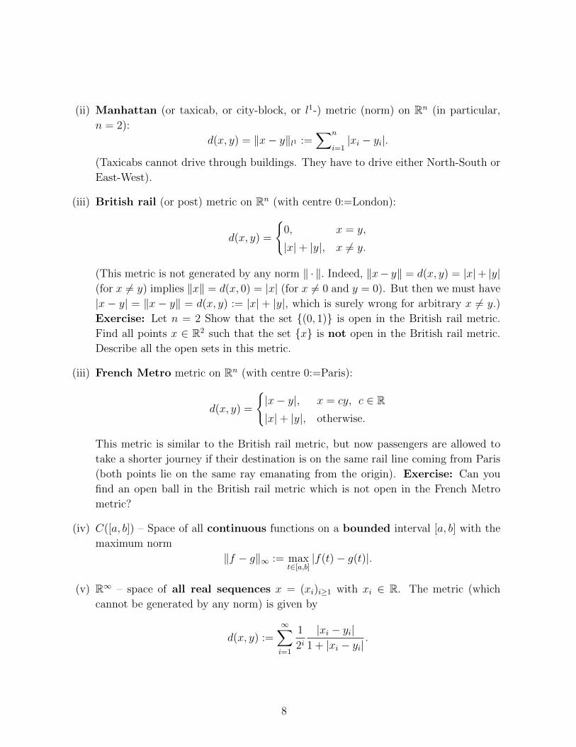
(ii) Manhattan (or taxicab, or city-block, or l1-) metric (norm) on Rn (in particular,
n = 2):
d(x, y) = ‖x− y‖l1 :=∑n
i=1|xi − yi|.
(Taxicabs cannot drive through buildings. They have to drive either North-South or
East-West).
(iii) British rail (or post) metric on Rn (with centre 0:=London):
d(x, y) =
0, x = y,
|x|+ |y|, x 6= y.
(This metric is not generated by any norm ‖ · ‖. Indeed, ‖x− y‖ = d(x, y) = |x|+ |y|(for x 6= y) implies ‖x‖ = d(x, 0) = |x| (for x 6= 0 and y = 0). But then we must have
|x − y| = ‖x − y‖ = d(x, y) := |x| + |y|, which is surely wrong for arbitrary x 6= y.)
Exercise: Let n = 2 Show that the set (0, 1) is open in the British rail metric.
Find all points x ∈ R2 such that the set x is not open in the British rail metric.
Describe all the open sets in this metric.
(iii) French Metro metric on Rn (with centre 0:=Paris):
d(x, y) =
|x− y|, x = cy, c ∈ R|x|+ |y|, otherwise.
This metric is similar to the British rail metric, but now passengers are allowed to
take a shorter journey if their destination is on the same rail line coming from Paris
(both points lie on the same ray emanating from the origin). Exercise: Can you
find an open ball in the British rail metric which is not open in the French Metro
metric?
(iv) C([a, b]) – Space of all continuous functions on a bounded interval [a, b] with the
maximum norm
‖f − g‖∞ := maxt∈[a,b]
|f(t)− g(t)|.
(v) R∞ – space of all real sequences x = (xi)i≥1 with xi ∈ R. The metric (which
cannot be generated by any norm) is given by
d(x, y) :=∞∑i=1
1
2i|xi − yi|
1 + |xi − yi|.
8

(vi) l∞ – the space of all bounded sequences
l∞ :=
x = (xi)i≥1 ∈ R∞
∣∣∣∣ supi≥1|xi| <∞
with d(x, y) := ‖x− y‖∞ := sup
i≥1|xi − yi|.
(vii) The space of p-summable sequences lp, 1 ≤ p <∞,
lp :=
x = (xi)i≥1 ∈ R∞
∣∣∣∣∣∞∑i=1
|xi|p <∞
with the norm ‖x‖p := p
√√√√ ∞∑i=1
|xi − yi|p.
The triangle inequality for ‖ · ‖p is known as Minkovski’s inequality(∞∑i=1
|xi + yi|p)1/p
≤
(∞∑i=1
|xi|p)1/p
+
(∞∑i=1
|yi|p)1/p
, x, y ∈ lp.
Closely related is Holder’s inequality for sequences
∞∑i=1
|xiyi| ≤
(∞∑i=1
|xi|p)1/p
·
(∞∑i=1
|yi|q)1/q
,
x ∈ lp, y ∈ lq,1
p+
1
q= 1 (p, q > 1).
Exercise 1.1.21. Check that the following define metrics on the set of all positive
integers N := 1, 2, 3, . . .:
(i) ρ(n,m) = |m−n|mn
;
(ii) ρ(n,m) =
0, m = n;
1 + 1m+n
, m 6= n.
1.2 Sequences and Convergence
Definition 1.2.1. Let (X, d) be a metric space and (xn)n∈N be a sequence in X. We
say that xn converges to some x ∈ X if
∀ε > 0, ∃N(ε) ∈ N, ∀n > N(ε) : d(xn, x) < ε.
9
Notation 1.2.2. We write xn → x or limn→∞ xn = x.
In other words: xn ∈ Bε(x) for all n > N(ε);
or equivalently, xn → x⇐⇒ d(xn, x)→ 0 (in the sense of real numbers)
Theorem 1.2.3 (Uniqueness of limits). A sequence (xn)n∈N has at most one limit.
Proof. Suppose not, and
limn→∞
xn = x, limn→∞
xn = y, x 6= y.
Let
ε := d(x, y)/2 > 0.
Then:
∃N1(ε) : d(xn, x) < ε ∀n > N1(ε);
∃N2(ε) : d(xn, y) < ε ∀n > N2(ε).
Put N := maxN1(ε), N2(ε). Then for n > N : d(xn, x), d(xn, y) < ε.
d(x, y) ≤ d(xn, x) + d(xn, y) < 2ε = d(x, y),
which is a contradiction with d(x, y) > 0.
Theorem 1.2.4. If (xn)n∈N converges, then (xn)n∈N is bounded.
Proof. Choose ε = 1 in the definition of convergence. There exists N0 ∈ N such that
d(xn, x) < 1 for n > N0. Let
R := 1 + max1≤n≤N0
d(xn, x).
Then d(xn, x) ≤ R for all n ∈ N i.e.,
(xn)n∈N ⊆ BR(x).
Remark 1.2.5. In the discrete space X (see Example 1.1.2), any convergent sequence
is ‘eventually stationary’:
limn→∞
xn = x ⇐⇒ ∃N0 ∈ N : xn = x ∀n > N.
Definition 1.2.6. x ∈ X is a cluster point of (xn)n∈N if for any (small) open ball
with center at x, the sequence returns infinitely often to the ball.
10

In other words,
∀ε > 0, ∀N ∈ N, ∃n = n(ε) > N : d(xn, x) < ε.
Remark 1.2.7. This is a weaker condition than convergence: we may have an infinite
number of terms outside the ball Bε(x). The limit of the sequence is always a cluster
point, but the converse need not be true.
Example 1.2.8. Let X = R and
xn =
0, n even (n = 2m),
1, n odd (n = 2m+ 1).
(xn)n∈N has 2 cluster points, 0 and 1.
Example 1.2.9. Let X = R and
xn = (0, 0, 1, 0, 1, 2, 0, 1, 2, 3, 0, 1, 2, 3, 4, 0, 1, 2, 3, 4, 5, . . .)
(xn)n∈N has infinitely many cluster points, 0, 1, 2, 3, . . ..
Exercise 1.2.10. Show that the sequence
xn = (−1)n(
1− 1
n
)does not converge in R. Find all cluster points of the sequence.
Theorem 1.2.11. x is a cluster point of (xn)n∈N if and only if there exists a subse-
quence (xnm)m∈N of (xn)n∈N such that limm→∞ xnm = x.
Proof. We give only a sketch.
(⇐=) is trivial.
(=⇒) Choose a sequence of balls Bεm(x) with εm ↓ 0. For each m find some xnm ∈Bεm . Make sure that nm+1 > nm (this is always possible since Bεm(x) contains
infinitely many elements of (xn)n∈N). Then xnm → x as m→∞.
Exercise 1.2.12. Find cluster points of the following sequences in R:
(i) xn = (−1)n;
(ii) xn = sin(π2n);
(iii) xn =
2− 1
n, n even,
1/n, n odd;
(iv) xn = n mod 4.
11

1.3 Open and Closed Sets
Recall the definition of an open set from Section 1.1.
Theorem 1.3.1. Let (X, d) be a metric space. Then:
(i) ∅ and X are open and closed (simultaneously);
(ii) The intersection of any finite collection of open sets is open;
(iii) The union of any arbitrary (possibly infinite) collection of open sets is open.
Exercise 1.3.2. Prove this theorem.
Example 1.3.3. We’ll show why point (ii) of Theorem 1.3.1 does not necessarily
apply to infinite intersections. Consider open balls in Rn, n ≥ 1,
Bεn(x0) with some x0 ∈ Rn and εn = 1/n.
Then the countable intersection ⋂n∈N
Bεn(x0) = x0
is not open in Rn.
Definition 1.3.4. Let (X, d) be a metric space, and A ⊆ X (a subset of X).
(i) A point x ∈ A is an interior point of A if Bε(x) ⊆ A for some ε > 0. The
interior of A, which will be denoted by intA or A, is the set of all interior
points of A.
(ii) x ∈ X (possibly, x /∈ A) is a closure point of A if
Bε(x) ∩ A 6= ∅ for all ε > 0.
The closure of A, which will be denoted by A, consists of all closure points of
A. Obviously, A ⊆ A (since Bε(x) ∩ A 3 x for each x ∈ A).
(iii) x ∈ X is a boundary point of A if for all ε > 0:
Bε(x) ∩ A 6= ∅ and Bε(x) ∩ Ac 6= ∅.
The boundary of A, denoted by ∂A, consists of all boundary points of A.
x ∈ ∂A ⇐⇒ x ∈ A ∩ Ac.
12
From the above definitions
A ⊆ A ⊆ A, A = A ∪ ∂A = A ∪ ∂A, ∂A = A\A = A ∩ Ac.
In particular, the closure of the open ball Bε(x) is always contained in the closed ball
Bε(x), see Definition 1.1.11. Furthermore, in the Euclidean space Rn they coincide.
Remark 1.3.5. In general, the closure of Bε(x) does not coincide with the closed
ball Bε(x)! A typical counterexample is the discrete metric with the unit open ball
B1(x) = x (which is an open and closed set simultaneously) and the closed ball
B1(x) = X.
Theorem 1.3.6. Let (X, d) be a metric space. Then:
(i) A is the largest open set contained in A;
(ii) A is open ⇐⇒ A = A;
(iii) A is the smallest closed set containing A;
(iv) A is closed ⇐⇒ A = A
Proof. We will prove only (i), (ii).
(i) Show first that A is open. By definition, for any x ∈ A there exists Bε(x) ⊂ A.
We claim that indeed Bε(x) ⊂ A. Pick an arbitrary y ∈ Bε(x). Since Bε(x) is
an open set, there exists η > 0 such that
Bη(y) ⊂ Bε(x) ⊂ A.
This means that any y ∈ Bε(x) is an interior point of A, i.e., Bε(x) ⊂ A.
Show next that A is the largest open subset of A: If B ⊆ A and B is open,
then B ⊆ A. Indeed, for every point x ∈ B one finds a ball Bε(x) ⊂ B ⊂ A,
which means x ∈ A.
(ii) If A = A, then A is open, because A is always open by Claim (i). If A is open,
then any x ∈ A is an interior point, which implies A ⊆ A ⊆ A.
Exercise 1.3.7. Prove Claims (iii) and (iv). Hint: use that A open ⇐⇒ Ac closed.
The next theorem is very important!
Theorem 1.3.8 (Characterization of Closed Sets). A set A ⊆ X is closed if and
only if any convergent sequence in X, (xn)n∈N ⊂ A has its limit inside A, i.e.,
∃ limn→∞
xn := x ∈ X =⇒ x ∈ A.
13
Proof. (=⇒) Let A be closed and x := limn→∞ xn ∈ X. Suppose x /∈ A, i.e.,
x ∈ Ac := X\A, which is an open set. Therefore, Bε(x) ⊆ Ac for some ε > 0. By the
definition of convergence,
xn ∈ Bε(x) ⊆ Ac, ∀n > N(ε) ∈ N.
This contradicts the assumption (xn)n∈N ⊆ A.
(⇐=) We show that Ac is open. So, let x ∈ Ac, i.e., x /∈ A. If Bε(x) * Ac for any
ε > 0, i.e., Bε(x) ∩ A 6= ∅, we can pick a sequence xn ∈ Bεn(x) ∩ A with εn ↓ 0,
n → ∞. By construction, (xn)n∈N ⊂ A and limn→∞ xn = x. By assumption we
should have that x ∈ A, which is a contradiction with x /∈ A.
Exercise 1.3.9. Show that any closed ball Bε(x) is a closed set. Hint: use Theorem
1.3.8. Indeed, let (xn)n∈N ⊂ Bε(x) be convergent to some y ∈ X. Then by the triangle
inequality, for any n ∈ N
d(x, y) ≤ d(x, xn) + d(xn, y) ≤ R + d(xn, y).
Since d(xn, y)→ 0 as n→∞, this yields d(x, y) ≤ R.
Exercise 1.3.10. Let A ⊆ X be closed and x /∈ A. Show that
d(x,A) := infy∈A
d(x, y) > 0
Hint: what happens if we suppose the converse is true?
1.4 Limits of Functions, Continuity
Definition 1.4.1 (Continuous functions). Let (X, d) and (Y, ρ) be two metric spaces.
Let f : X → Y be a function (also called a map or mapping). We say that f is
continuous at a point x0 ∈ X if
∀ε > 0, ∃δ > 0 : d(x, x0) < δ =⇒ ρ(f(x), f(x0)) < ε.
We say that f is continuous if it is continuous at every point x0 ∈ X.
Intuition: you can control the changes of f : a “small” change in x away from x0
will not change f(x0) too much.
The following is an equivalent definition of continuity.
Definition 1.4.2 (Continuous functions in terms of open balls).
∀ε > 0 ∃δ > 0 : f(x) ∈ Bε(f(x0)) for all x ∈ Bδ(x0).
14

Note that in the above definition δ := δ(ε, x0), i.e., it depends on ε as well as on the
point x0.
History: This (ε, δ)-definition is due to A.-L. Cauchy (1789-1857), the French mathe-
matician who was an early pioneer of analysis. He had more than 800 research papers
and became a full professor of Ecole Polytechnique at 28 years old. Cauchy’s inspi-
ration for continuity came from properties of differentiable functions. It was thought
for a very long time that all continuous functions were differentiable (except possibly
on a set of isolated points). Weierstrass proved that this was not true in 1872 when
he gave an example of a continuous function that was differentiable nowhere.
Exercise 1.4.3. Let y ∈ X be fixed. Show that the distance function f defined by
(X, d) 3 x→ f(x) := d(x, y) ∈ R
is continuous.
Theorem 1.4.4 (Sequential Characterization of Continuity). The function f : X →Y is continuous at the point x0 ∈ X if and only if for every sequence (xn)n∈N ⊆ X
converging to x0, the sequence (f(xn))n∈N ⊆ Y is convergent to f(x0) ∈ Y .
Symbolically: limn→∞
xn = x0 =⇒ limn→∞
f(xn) = f(x0).
Proof. (=⇒) Suppose f is continuous at a point x0 ∈ X. Let xn → x0 as n → ∞.
For a given ε > 0, choose δ = δ(ε) > 0 such that ρ(f(x), f(x0)) < ε for all x ∈ Xwith d(x, x0) < δ. By the definition of limn→∞ xn = x0,
∃N(δ) ∈ N : d(xn, x0) < δ for all n > N(δ).
Hence,
ρ(f(xn), f(x0)) < ε for all n > N(δ).
Therefore, f(xn) −→ f(x0) as n→∞.
(⇐=) Proof by contradiction: Suppose f is not continuous at x0 ∈ X. Then ∃ε > 0
such that ∀δ > 0 one finds xδ ∈ X with d(xδ, x0) < δ but ρ(f(xδ), f(x0)) ≥ ε. Now
let δn = 1/n and choose the corresponding sequence
xn := xδn , n ∈ N.
Then xn → x0, but f(xn) 9 f(x0) as n→∞.
So, the (ε, δ)-definition of continuity is equivalent to the sequential definition.
History: The notion of sequential continuity is due to the German mathematician
Heinrich Heine (1821-81).
15

Theorem 1.4.5 (Composition of Continuous Functions). Let (X, d1), (Y, d2), and
(Z, d3) be metric spaces. Let f : X → Y and g : Y → Z be functions such that f is
continuous at some point x0 ∈ X and g is continuous at y0 := f(x0) ∈ Y . Then,
their composition
h := g f : X → Z
is continuous at x0.
Proof. We use the characterization of continuity in terms of sequences. Let xn → x0
as n → ∞. As f is continuous, yn := f(xn) → f(x0) =: y0. As g is continuous,
zn := g(yn)→ g(y0) = g(f(x0)) =: z0 ∈ Z as n→∞.
The next theorem is one of the most important characterisations of continuity and
it should be memorised!
Theorem 1.4.6 (Global Continuity). The function f : X → Y is continuous if and
only if the preimage
f−1(U) := x ∈ X | f(x) ∈ U
of any open set U ⊆ Y is open in X.
Proof. (=⇒) Let f : X → Y be continuous on X. Let U be an open subset of Y , we
check that that f−1(U) is open. Take any x0 ∈ f−1(U), then f(x0) ∈ U . As U is
open, there exists ε > 0 such that Bε(f(x0)) ⊆ U . As f is continuous at x0, there
exists δ > 0 such that
f(Bδ(x0)) ⊆ Bε(f(x0)) ⊆ U,
or
Bδ(x0) ⊆ f−1(U).
This means that f−1(U) is open.
(⇐=) Let x0 ∈ X and ε > 0. By assumption, f−1 [Bε(f(x0))] ⊆ X is open
as the preimage of the open ball Bε(f(x0)). Hence ∃δ > 0 such that Bδ(x0) ⊆f−1 [Bε(f(x0))], or f(Bδ(x0)) ⊆ Bε(f(x0)). This gives the required continuity of
f .
Corollary 1.4.7. Let f : (X, d)→ (R, | · |) be continuous. Then for any C ∈ R
x ∈ X | f(x) > C is open,
x ∈ X | f(x) ≤ C is closed.
There is an equivalent formulation of Theorem 1.4.6 in terms of closed sets.
16

Corollary 1.4.8. The function f : X → Y is continuous ⇐⇒ the preimage f−1(B)
of any closed set B ⊆ Y is closed in X.
Exercise 1.4.9. Prove the above corollary using Theorem 1.4.6 and the equality
[f−1(U)]c = f−1(U c)
for any subset U ⊆ Y .
Warning: A similar statement for images of open (resp. closed) sets is in general
wrong! If V ⊆ X is open (resp. closed) in X, then
f(V ) := y ∈ Y | y := f(x), x ∈ V
is not necessarily open (resp. closed) in Y .
Exercise 1.4.10. Find an example of a continuous function f : X → Y and an open
subset U ⊆ X such that f(U) is not an open subset of Y .
Definition 1.4.11. Let (X, d) and (Y, ρ) be two metric spaces. A function f : X → Y
is uniformly continuous if
∀ε > 0, ∃δ > 0 : ρ(f(x1), f(x2)) < ε, ∀x1, x2 ∈ X with d(x1, x2) < δ.
Remark 1.4.12. δ := δ(ε) is independent of points x ∈ X, unlike in the (ε, δ)-
definition of continuity.
The following generalisations of continuity are important but will not be examinable:
Definition 1.4.13. Let (X, ‖ · ‖X) and (Y, ‖ · ‖Y ) be two normed spaces. A function
f : X → Y is Lipschitz-continuous if there exists a (Lipschitz) constant L > 0
such that
‖f(x1)− f(x2)‖Y ≤ L‖x1 − x2‖X , ∀x1, x2 ∈ X.Lemma 1.4.14. Lipschitz-continuous functions are uniformly continuous.
Proof. Let ε > 0 and set δ := ε/L > 0. Then for any x1, x2 ∈ X with ‖x1−x2‖X < δ
dY (x1, x2) := ‖f(x1)− f(x2)‖Y ≤ L‖x1 − x2‖X < Lδ = ε.
The following definition is a generalisation of Lipschitz continuity.
Definition 1.4.15. Let (X, ‖ · ‖X) and (Y, ‖ · ‖Y ) be two normed spaces. A function
f : X → Y is Holder-continuous (with exponent α) if there exist α,L > 0 such
that
‖f(x1)− f(x2)‖Y ≤ L‖x1 − x2‖αX , ∀x1, x2 ∈ X.
Holder-continuous functions are also uniformly continuous.
17
1.5 Cauchy Sequences, Complete Metric Spaces
Definition 1.5.1. Let (X, d) be a metric space. A sequence (xn)n∈N ⊆ X is a
Cauchy sequence if
∀ε > 0, ∃N(ε) ∈ N, ∀m,n > N(ε) : d(xm, xn) < ε.
Intuition: A sequence is Cauchy if its terms get closer and closer to each other.
Theorem 1.5.2. Every convergent sequence in (X, d) is Cauchy.
Proof. Let xn → x as n→∞. Then ∀ε > 0, ∃N(ε) > 0 such that
d(xn, x) < ε/2, ∀n > N(ε).
Hence, for any n,m > N(ε)
d(xn, xm) ≤ d(xn, x) + d(x, xm) < ε.
Warning: In general metric spaces, the converse claim is false!
Definition 1.5.3. A metric space (X, d) is called complete if every Cauchy sequence
(xn)n∈N in X converges to some x ∈ X.
A normed space (X, ‖·‖X) that is complete w.r.t. the metric dX(x1, x2) := ‖x1−x2‖Xis called a Banach space.
Exercise 1.5.4. Every Cauchy sequence in (X, d) is bounded (compare with Theorem
1.2.4).
Exercise 1.5.5. Let (X, d) be a complete metric space and Y ⊆ X. Then
(Y, d) is complete ⇐⇒ Y is a closed set in (X, d).
1.6 Banach Contraction Mapping Theorem
Definition 1.6.1. Let (X, d) be a metric space. A function
T : X → X
sending X into X is called an operator in X. An operator T is a contraction of
modulus β ∈ (0, 1) if
d(Tx, Ty) ≤ β · d(x, y), ∀x, y ∈ X.
18

Exercise 1.6.2. Show that every contraction is a uniformly continuous function.
The next theorem is possibly the most important result in this course and it should be
memorised! It is used throughout analysis, the study of differential equations, matrix
analysis, game theory, dynamical systems and many other areas of mathematics and
economics.
Theorem 1.6.3 (Banach Contraction Mapping Theorem). Let (X, d) be a complete
metric space and T : X → X be a contraction of modulus β ∈ (0, 1). Then:
(i) T has exactly one fixed point x∗ ∈ X solving the equation
Tx = x.
(ii) How to construct x∗: For any starting point x0 ∈ X, the sequence (xn)n∈Ndefined by
x1 := Tx0, x2 := Tx1, . . . , xn+1 := Txn, . . . (∗)
converges to x∗.
Proof. It is useful to prove the existence of the fixed point and its uniqueness sepa-
rately.
(ia) Existence: Take any x0 ∈ X and define (xn)n∈N as in (∗). We show that this
sequence is Cauchy:
d(xn+1, xn) = d(Txn, Txn−1) ≤ βd(Txn, Txn−1)
≤ . . . ≤ βnd(Tx1, Tx0), n ∈ N.
Then, by the triangle inequality, for any n > m
d(xn, xm) ≤n−1∑i=m
d(xi+1, xi) ≤
(n−1∑i=m
βi
)· d(x1, x0) ≤
(∞∑i=m
βi
)· d(x1, x0)
(geometric series) ≤ βm
1− βd(x1, x0)→ 0 as m→∞ (since βm → 0).
Since (X, d) is complete =⇒ ∃x∗ := limn→∞ xn. We show that this x∗ is a fixed
point of T . Recall that T is continuous as it is a contraction (see Exercise 1.6.2
and Theorem 1.4.4). Indeed,
Tx∗ = T ( limn→∞
xn) = limn→∞
Txn = limn→∞
xn+1 = x∗.
19
(ib) Uniqueness: Let x, y ∈ X be two fixed points. T is a contraction with β <
1 =⇒
d(x, y) = d(Tx, Ty) ≤ βd(x, y),
i.e., d(x, y) = 0 ⇐⇒ x = y.
(ii) As was shown in (ia), any sequence of the form (∗) converges to some fixed point
x∗ (possibly depending on the initial point x0). But according to (ib), the fixed
point is unique, which means that each approximating sequence (xn)n∈N has the
limit x∗, which is the same for all x0 ∈ X.
Exercise 1.6.4. Let (X, d) be a complete metric space, and let T : X → X be such
that, for some n ∈ N, the operator T n is a contraction. Show that T has a unique
fixed point.
Hint: (i) Prove that T n has a unique fixed point, say x∗. (ii) Check that this x∗ is
also the unique fixed point for T .
The Banach fixed point theorem is one of the most important theorems in all of
mathematics! Many problems can be formulated as equations F (x) = 0 and can be
rewritten in the form f(x) = x with f(x) := F (x) + x.
Standard applications of the Banach fixed point theorem include:
— The Picard-Lindelof theorem about unique solvability of ordinary differential equa-
tions.
— The Page rank algorithm used by Google: One computes a fixed point of a linear
operator in RN (with huge N →∞), which is a contraction. This fixed point x∗ ∈ RN
gives ordering of pages.
— Image compression: Digital encoding of images in the JPEG format is also a
mathematical algorithm based on the Banach fixed point theorem.
Theorem 1.6.5 (Continuous Dependence of the Fixed Point on Parameters). Let
(X, d) and (Ω, ρ) be metric spaces, and T (x, ω) be a mapping X × Ω→ X. Further-
more, let (X, d) be complete. Suppose that for each x ∈ X
Ω 3 ω → T (x, ω) ∈ X is continuous,
and for each ω ∈ Ω
X 3 x→ T (x, ω) ∈ X is a contraction with (the same) β ∈ (0, 1).
20
Then the solution x∗(ω) ∈ X of the fixed point problem
T (x, ω) = x
is a continuous function of the parameter ω ∈ Ω.
Proof. Let ωn → ω in (Ω, ρ). We need to show that
d(x∗(ωn), x∗(ω))→ 0, as n→∞.
Denote the corresponding fixed points
x∗ : = x∗(ω) = T (x∗(ω), ω) = T (x∗, ω),
x∗n : = x∗(ωn) = T (x∗(ωn), ωn) = T (x∗n, ωn).
Thus, by the triangle inequality
d(x∗n, x∗) = d(T (x∗, ω), T (x∗n, ωn))
≤ d(T (x∗, ω), T (x∗, ωn)) + d(T (x∗, ωn), T (x∗n, ωn))
≤ d(T (x∗, ω), T (x∗, ωn)) + β · d(x∗, x∗n),
which can be rewritten as
(1− β)d(x∗n, x∗) ≤ d(T (x∗, ω), T (x∗, ωn))
or
d(x∗n, x∗) ≤ 1
1− βd(T (x∗, ω), T (x∗, ωn)).
Since T (x∗, ω) is continuous in ω, the right-hand side tends to zero as ωn → ω. Thus,
d(x∗n, x∗) as n→∞.
Exercise 1.6.6. Let (X, d) be a complete metric space. Suppose we have two con-
tractions A : X → X and B : X → X such that
d(Ax,Ay) ≤ αd(x, y), d(Bx,By) ≤ βd(x, y), with α, β ∈ (0, 1).
Prove that, if for some ε > 0
d(Ax,Bx) < ε for all x ∈ X,
then the fixed points x∗ and y∗ obey
d(x∗, y∗) ≤ ε
1− γ, γ := maxα, β < 1.
21

Exercise 1.6.7. On a calculator, if you enter any number x0 and then apply the
cos function to x0, you get a new number x1 := cos x0. If we iterate this process
xn+1 := cosxn, you’ll find that the sequence of values xn converges to some other value
x∞ ' 0.739085133 . . .. Show that the function g : [0, 1]→ [0, 1] given by g(x) = cos x
is a contraction (you might need to use the Mean Value Theorem). Interpret this
property of the cosine function in terms of the Banach fixed point theorem. Why does
this justify the method of iterating the cos function on a calculator to show that the
sequence xn converges? How many roots does the function f(x) = cosx− x have in
the interval [0, 1]?
1.7 Cantor Intersection Theorem
Theorem 1.7.1 (Cantor Intersection Theorem1). A metric space (X, d) is complete
if and only if any decaying sequence of non-empty closed sets
∅ 6= An = An ⊆ X, An+1 ⊆ An, n ∈ N,
with diameters decaying to zero
diamAn := sup d(x, y) | x, y ∈ An → 0, n→∞,
has exactly one common point
x ∈⋂n∈N
An (i.e.,⋂n∈N
An = x).
Proof. (=⇒) Suppose X is complete and consider any decaying sequence (An)n∈N ⊆X as described above. Since An 6= ∅ =⇒ ∃xn ∈ An. Obviously, xm ∈ Am ⊆ An for
all m ≥ n, and hence
d(xn, xm) ≤ diamAn, m ≥ n.
So, (xn)n∈N is a Cauchy sequence as diamAn → 0. Since X is complete =⇒
∃ limn→∞
xn =: x ∈ X.
We claim that x ∈⋂n∈NAn. Indeed, xm ∈ An for all m ≥ n and An is closed, thus
by the characterisation of closed sets (Theorem 1.3.8), x = limm→∞, m≥n
xm = x ∈ An.
So, x ∈⋂n∈NAn.
1Georg Cantor (1845–1918), German mathematician, inventor of set theory
22

Finally, we observe that⋂n∈NAn consists only of the unique point x. If y 6= x is
some other point from⋂n∈NAn, then
d(x, y) ≤ diamAn → 0, n→∞,
which yields x = y.
(⇐=) This is left as an optional exercise. It is not so trivial. Argue by contradiction.
1.8 Separable Spaces
Definition 1.8.1. A subset A ⊆ X is called dense in (X, d) if its closure is the
whole of X, i.e.,
A = X.
Example 1.8.2. Let X = [0, 1] and let A = (0, 1). Clearly A ⊂ A. Also, the points
0 and 1 are in the closure of A, as the sequence xn := 1n⊂ A converges to 0 and the
sequence xm := 1− 1m⊂ A converges to 1. It follows that (0, 1) is dense in [0, 1].
Definition 1.8.3. A space (X, d) is called separable if there exists a countable set
(i.e., sequence)
A = (xn)n∈N ⊆ X,
which is dense in X.
In other words Definition 1.8.3 says that for each x ∈ X there exists a subsequence
(xnm)m∈N of (xn)n∈N such that
x = limm→∞
xnm ,
which means that x is a cluster point of (xn)n∈N. Or equivalently,
∀x ∈ X, ∀ε > 0, ∃xn ∈ A : d(xn, x) < ε;
or equivalently, ∀x ∈ X, ∀ε > 0 : A ∩Bε(x) 6= ∅.
Definition 1.8.4. A metric space is called a Polish space if it is complete and
separable.
23

1.9 Basic Examples revisited
(i) Euclidean space (Rn, | · |) of vectors x = (xi)ni=1 with metric
d(x, y) = |x− y| :=
√√√√ n∑i=1
(xi − yi)2.
This is a Polish (normed) space with the dense set Qn (consisting of vectors
with rational components xi ∈ Q).
(ii) Manhattan (or taxicab, or city-block, or l1-) metric (norm) on Rn (in partic-
ular, n = 2):
d(x, y) = ‖x− y‖l1 :=∑n
i=1|xi − yi|.
(We cannot cut the corners and walk along the streets). Again this is a separable
Banach space.
(iii) British rail (or post) metric on Rn (with centre 0:=London):
d(x, y) =
0, x = y,
|x|+ |y|, x 6= y.
Exercise: Show that Euclidean space with the British rail metric is complete
but not separable. (Hint: recall that for every x 6= 0, the set x is open).
(iii) French Metro metric on Rn (with centre 0:=Paris):
d(x, y) =
|x− y|, x = cy, c ∈ R|x|+ |y|, x 6= y.
Exercise: Show that Euclidean space with the French Metro metric is not
separable. (Hint: think in polar coordinates)
(iv) C([a, b]) – Banach space of all continuous functions on a bounded interval
[a, b] with the maximum norm
‖f − g‖∞ := maxt∈[a,b]
|f(t)− g(t)|.
For completeness of C([a, b]) see Lemma 1.9.3 below. This space is separable:
for instance, A = C([a, b]), where A is the set of all polynomials with rational
coefficients;
P (t) := a0tN + a1t
N−1 + · · ·+ aN−1t+ aN , ai ∈ Q, N ∈ N.
24

(v) R∞ – space of all real sequences x = (xi)i≥1 with xi ∈ R. The metric (which
cannot be generated by any norm) is given by
d(x, y) :=∞∑i=1
1
2i|xi − yi|
1 + |xi − yi|.
This is a Polish space, a countable dense set A consists e.g. of all finite sequences
with rational coefficients (q1, q2, . . . , qN , 0, 0, . . .), qi ∈ Q, N ∈ N. For a sequence
(xn)n∈N ⊂ R∞ with xn = (xn,i)i≥1 = (xn,1, xn,2, . . . , xn,i, . . .),
d(xn, x) →n→∞
0 ⇐⇒ xn,i →n→∞
xi, ∀i ∈ N,
i.e., the convergence in the above metric d is equivalent to the coordinate
convergence for each fixed i.
(vi) l∞ – Banach space of all bounded sequences
l∞ :=
x = (xi)i≥1 ∈ R∞ | sup
i≥1|xi| <∞
with d(x, y) := ‖x− y‖∞ := sup
i≥1|xi − yi|.
xn →n→∞
x in l∞ ⇐⇒ coordinate convergence xn,i →n→∞
xi
uniformly w.r.t i ∈ N,i.e., sup
i∈N|xn,i − xi| → 0 as n→∞.
Warning! This space is complete but not separable! Define its subset
B := x = (xi)i∈N ∈ l∞ | xi = 0 or 1 for each i ∈ N .
This subset is not countable (its cardinality is that of the continuum). But
d(x, y) = 1 for all x, y ∈ B, x 6= y. If there exists a set A that is dense in l∞,
then in each of the balls B1/2(y), y ∈ B, there should be at least one point
x ∈ A. Such balls do not intersect, which means that A is also uncountable.
This contradicts the assumption that l∞ is separable.
(vii) Polish spaces of p-summable sequences lp, 1 ≤ p <∞,
lp :=
x = (xi)i≥1 ∈ R∞
∣∣∣∣∣∞∑i=1
|xi|p <∞
with the norm ‖x‖p := p
√√√√ ∞∑i=1
|xi − yi|p.
25
Exercise 1.9.1. (not trivial) Check completeness of lp.
(viii) Lp([a, b]) – Banach space of all Lebesgue p-integrable functions, 1 ≤ p <∞,
with
d(x, y) = ‖x− y‖Lp :=
(∫ b
a
|x(t)− y(t)|pdt)1/p
.
A dense set A is the set of all polynomials with rational coefficients.
Minkovski’s inequality for functions(∫ b
a
|x(t) + y(t)|pdt)1/p
≤(∫ b
a
|x(t)|pdt)1/p
+
(∫ b
a
|y(t)|pdt)1/p
.
Holder’s inequality for functions∫ b
a
|x(t)y(t)|dt ≤(∫ b
a
|x(t)|pdt)1/p
·(∫ b
a
|y(t)|qdt)1/q
x ∈ Lp, y ∈ Lq,1
p+
1
q= 1 (p, q > 1).
(ix) Ck([a, b]) for k = 1, 2, ..., Banach space of k-times continuously differen-
tiable functions x : [a, b]→ R, with the norm
‖x‖Ck :=k∑i=0
maxt∈[a,b]
|x(k)(t)|, x(0)(t) := x(t).
Again, a countable dense set in Ck([a, b]) are polynomials with rational coeffi-
cients.
General spaces of bounded continuous functions
Let (X, d) be a metric space. Define
Cb(X) := f : X → R | f is continuous and bounded on X
with the supremum (not maximum) norm
‖f‖Cb= ‖f‖∞ := sup
x∈X|f(x)|.
Compare:
(a) Cb((−∞,∞)) = Cb(R) with the sup-norm; but
26
(b) Cb([a, b]) with the max-norm (since max f = sup f on a bounded closed interval
[a, b]).
In general, we do not assume that X is compact (as will be introduced in Section
1.12).
The convergence of (fn)n∈N ⊂ Cb(X) to f ∈ Cb(X) in the sup-norm is equivalent to
the uniform convergence.
Definition 1.9.2. Let fn, f be functions on X. We say that fn → f uniformly
on X (notation: fn ⇒ f) as n→∞ if
∀ε > 0, ∃N(ε) ∈ N : |fn(x)− f(x)| < ε, ∀x ∈ Xas n > N(ε);
which implies ‖fn − f‖∞ := supx∈X|fn(x)− f(x)| ≤ ε (here ≤ and not <).
Lemma 1.9.3. Let a sequence (fn)n∈N ⊂ Cb(X) converge uniformly to some func-
tion f : X → R. Then certainly f ∈ Cb(X).
Proof. From the uniform convergence fn ⇒ f we have
∀ε > 0, ∃N ∈ N : supx∈X|fN(x)− f(x)| < ε/3.
Fix now some x ∈ X. Since fN ∈ Cb(X),
∃δ > 0 : d(x, y) < δ =⇒ |fN(x)− fN(y)| < ε/3.
Thus for all such y ∈ Bδ(x) and for N ∈ N as above
|f(x)− f(y)| ≤ |f(x)− fN(x)|+ |fN(x)− fN(y)|+ |fN(y)− f(y)| < ε,
which means that f is continuous at each x ∈ X.
Corollary 1.9.4. (Cb(X), ‖ · ‖∞) is complete.
Proof. Let (fn)n∈N ⊂ Cb(X) be Cauchy w.r.t. ‖·‖∞. Recall that any Cauchy sequence
is bounded, i.e.,
supn≥1‖fn‖∞ := C <∞.
Obviously (fn(x))n∈N ⊂ R is Cauchy for each fixed x ∈ X and hence
∃ limn→∞
fn(x) =: f(x) ∈ R.
27

Furthermore, for each x ∈ X
|f(x)| ≤ supn≥1|fn(x)| ≤ sup
n≥1‖fn‖∞,
i.e., ‖f‖∞ ≤ C.
The required continuity of f : X → R then follows from Lemma 1.9.3 as soon as we
check that fn ⇒ f on X.
So, it remains to prove that ‖f − fn‖∞ → 0 as n → ∞. Indeed, by the Cauchy
property of (fn)n∈N
∀ε > 0, ∃N(ε) ∈ N : |fn(x)− fm(x)| < ε/2, ∀n,m > N(ε), ∀x ∈ X.
Thus, for each fixed n > N(ε) and x ∈ X, in the above estimate we can pass to the
limit fm(x)→ f(x) as m→∞ and get
∀ε > 0, ∃N(ε) ∈ N : |fn(x)− f(x)| ≤ ε/2, ∀n > N(ε), ∀x ∈ X,i.e., ∀ε > 0, ∃N(ε) ∈ N : ‖f − fn‖∞ ≤ ε/2 < ε, ∀n > N(ε).
Warning: Pointwise convergence (fn)n∈N ⊂ Cb(X) to f : X → R does not guarantee
that f ∈ Cb(X).
Example 1.9.5. X = [0, 1], fn(x) := xn,
limn→∞
fn(x) = f(x) =
0, 0 ≤ x < 1,
1, x = 1.
So, fn → f pointwise, but f /∈ C[0, 1]. This immediately says us that fn cannot
converge uniformly on [0, 1], otherwise by Lemma 1.9.3 we should have f ∈ C[0, 1].
1.10 Linear Mappings (Operators) in Normed Spaces
Let (X, ‖ · ‖X) and (Y, ‖ · ‖Y ) be normed spaces, and let the mapping L : X → Y be
linear, i.e.,
L(αx+ βy) = αL(x) + βL(y), ∀x, y ∈ X, ∀α, β ∈ R,in particular, L 0︸︷︷︸
∈X
= 0︸︷︷︸∈Y
.
Theorem 1.10.1 (Characterisation of Continuous Linear Mappings). The following
are equivalent:
28
(i) L is uniformly continuous on X;
(ii) L is continuous on X;
(iii) L is continuous only at 0 ∈ X (or at some x ∈ X);
(iv) L is bounded, in the sense it has the bounded operator norm
‖L‖ = ‖L‖X→Y := sup‖x‖X≤1
‖Lx‖Y <∞;
(v) ∃C ∈ (0,∞): ‖Lx‖Y ≤ C‖x‖X , ∀x ∈ X.
Proof. (i) → (ii) → (iii) are all trivial.
(iii) → (iv) By continuity of L at x = 0
∃δ > 0 : ‖x‖X < δ =⇒ ‖Lx‖Y < 1.
Then ∀x ∈ X, ‖x‖X ≤ 1,∥∥∥∥δ2x∥∥∥∥X
≤ δ
2< δ =⇒ ‖Lx‖Y =
∥∥∥∥L(2
δ· δ
2x
)∥∥∥∥Y
=2
δ
∥∥∥∥L(δ2x)∥∥∥∥
Y
<2
δ.
(iv) → (v) Let x 6= 0, then
‖Lx‖Y = ‖x‖X ·∥∥∥∥L( x
‖x‖X
)∥∥∥∥Y
≤ ‖x‖X · ‖L‖.
(v) → (i) Let ‖Lx‖Y ≤ C‖x‖X , ∀x ∈ X. Then
‖Lx− Ly‖Y = ‖L(x− y)‖Y ≤ C‖x− y‖X , ∀x, y ∈ X.
The definition of uniform continuity follows with any ε > 0 and δ = ε/L > 0.
Example 1.10.2. Let X = C([a, b]) with ‖f‖∞ := maxt∈[a,b] |f(t)|.
Define I : C([a, b])→ R by
If :=
∫ b
a
f(t)dt (Riemannian integral).
The linear map I is continuous since
|I(f)| ≤∫ b
a
|f(t)|dt ≤ (b− a)‖f‖∞, i.e., ‖I‖ ≤ (b− a) <∞.
Actually, by taking f0(t) ≡ 1 with ‖f0‖∞ = 1, we see that I(f0) = (b− a) and hence
‖I‖ = (b− a).
29

Example 1.10.3. Let X = C1([0, 1]) with the same sup-norm ‖f‖∞.
Define D : C1([0, 1])→ C([0, 1]) by
Df := f ′ (derivative).
Then D is linear but not continuous!
Proof. Take
fn(t) := tn, t ∈ [0, 1].
Obviously, fn ∈ C1([0, 1]) and ‖fn‖∞ = 1. But
Dfn(t) = ntn−1 = nfn−1(t)
and
‖Dfn‖∞ = n.
So,
‖D‖ := supf∈C1, ‖f‖∞≤1
‖Df‖∞ ≥ supn‖Dfn‖∞ =∞.
Aside: Equivalent definitions of the operator norm
Above we have defined the operator norm of L as
‖L‖ = ‖L‖X→Y := sup‖x‖X≤1
‖Lx‖Y . (∗)
In the literature you can also meet the following definitions
‖L‖ := sup‖y‖=1
‖Ly‖Y , (∗∗)
‖L‖ := supz 6=0
‖Lz‖Y‖z‖X
. (∗ ∗ ∗)
We claim all three definitions are equivalent.
Indeed, by the linearity of L
supz 6=0
‖Lz‖Y‖z‖X
= supz 6=0
∥∥∥∥L( z
‖z‖X· ‖z‖X
)∥∥∥∥Y∥∥∥∥ z
‖z‖X· ‖z‖X
∥∥∥∥X
= supz 6=0
‖z‖X ·∥∥∥∥L( z
‖z‖X
)∥∥∥∥Y
||z‖X ·∥∥∥∥ z
‖z‖X
∥∥∥∥X
= sup‖y‖X=1
‖Ly‖Y‖y‖X
= sup‖y‖X=1
‖Ly‖Y ≤ sup0≤‖x‖X≤1
‖Lx‖Y = sup0<‖x‖X≤1
‖Lx‖Y
30

(since L0 = 0). Note that for each x ∈ X with 0 < ‖x‖X ≤ 1
‖Lx‖Y =
∥∥∥∥L(‖x‖X · x
‖x‖X
)∥∥∥∥Y
= ‖x‖X︸ ︷︷ ︸≤1
∥∥∥L( x‖x‖X
)∥∥∥Y
≤∥∥∥L( x
‖x‖X
)∥∥∥Y
= ‖Ly‖Y ,
where
y :=x
‖x‖X∈ X obeys ‖y‖X = 1.
Hence,
sup‖y‖=1
‖Ly‖Y ≤ sup0<‖x‖X≤1
‖Lx‖Y ≤ sup‖y‖=1
‖Ly‖Y .
So, we have proved that
supz 6=0
‖Lz‖Y‖z‖X
= sup‖x‖X≤1
‖Lx‖Y = sup‖y‖=1
‖Ly‖Y .
1.11 Compact Sets (Heine-Borel, Bolzano-Weierstrass)
Definition 1.11.1. Let A ⊆ X
(i) An open cover of A is a family of open sets (Ui)i∈I ⊆ X (indexed by an
arbitrary set I) such that
A ⊆⋃i∈I
Ui.
(ii) A is compact if every open cover (Ui)i∈I of A has a finite subcover
A ⊆⋃
1≤k≤N
Uik = Ui1 ∪ · · · ∪ UiN .
Example 1.11.2. Let (xn)n≥1 be a convergent sequence in X with limn→∞
xn = x. Then
A := xnn≥1 ∪ x
is compact.
Proof. Let (Ui)i∈I be an open cover of A. Since
x ∈ A ⊆⋃i∈I
Ui =⇒ x ∈ Ui0 for some i0 ∈ I.
As Ui0 is open, we can find ε > 0 such that x ∈ Bε(x) ⊆ Ui0 . As xn → x, there exists
N0 ∈ N such that
xn ∈ Bε(x) ⊆ Ui0 for all n > N0.
31

Now choose some sets from the open cover such that Uin 3 xn, 1 ≤ n ≤ N0. Then
A ⊆⋃
0≤k≤N0
Uik = Ui0 ∪ Ui1 ∪ · · · ∪ UiN .
Warning: Without the limit point x the argument would not work! Indeed, see
the counterexample below:
Exercise 1.11.3. Show that the set A = 1/nn≥1 is not compact in R.
Hint: Consider e.g. the following open cover⋃n∈N Un ⊇ A:
U1 =
(1
2, 2
)3 1, Un =
(1
n+ 1,
1
n− 1
)3 1/n, n ≥ 2.
Theorem 1.11.4. Any compact set is closed and bounded.
Proof. We first show that Ac := X \ A is open—hence that A is closed. Take any
x ∈ Ac and define a family of open sets
Un := y ∈ X | d(y, x) > 1/n =[B1/n(x)
]c, n ∈ N.
By construction, U1 ⊆ · · · ⊆ Un ⊆ Un+1 ⊆ · · · and
A ⊆ X\x =∞⋃n=1
Un.
Since A is compact, there exists a finite subcover
A ⊆N⋃k=1
Unk.
Thus,
A ⊆ UK =[B1/K(x)
]cwith K = maxn1, . . . , nN,
or B1/K(x) ⊆ B1/K(x) ⊆ Ac.
(Note that A ⊆ B ⇐⇒ Bc ⊆ Ac.) Since x ∈ Ac is arbitrary, this means that Ac is
open.
We now show that A is bounded. Take any x ∈ A, then
A ⊆ X =∞⋃n=1
Bn(x).
32

By compactness,
A ⊆ Bn1(x) ∪ · · · ∪BnN(x).
Then
A ⊆ BK(x) with K = maxn1, . . . , nN,
which means that A is bounded.
Theorem 1.11.5. Let A ⊆ K ⊆ X, where K is compact and A = A is closed in X.
Then A is also compact.
Proof. By our assumption Ac := X\A is open. Let (Ui)i∈I be an open cover of A.
Then (Ui)i∈I and Ac together constitute an open cover of K. Since K is compact,
there exists a finite subcover
K ⊆ Ui1 ∪ · · · ∪ UiN ∪ Ac.
As A ⊆ K and A ∩ Ac = ∅, this yields A ⊆ Ui1 ∪ · · · ∪ UiN .
The next theorem is a famous and very important result which allows one to more
easily determine exactly when a subset of Euclidean space is compact. It should be
memorised!
Theorem 1.11.6 (Heine-Borel). Let A ⊆ Rn. Then
A is compact ⇐⇒ A is closed and bounded.
Proof. (=⇒) already done in Theorem 1.11.4.
(⇐=) Idea: LetA = A and A be bounded. Then there exists a quader [a, b]n ⊇ A.
By Th. 1.18 it would suffice to show that this quader is a compact set in Rn. We omit
the proof here (which is based on Cantor’s intersection theorem, cf. Th. 1.14).
Warning: This theorem (more precisely, its sufficient part) holds only in Rn or in
finite dimensional spaces, see Riescz Theorem below.
Definition 1.11.7. A set A ⊆ X is called sequentially compact if every sequence
(xn)n≥1 ⊆ A has a convergent subsequence (xnk)k≥1 whose limit belongs to A:
∃ limk→∞
xnk=: x ∈ A.
In other words, every (xn)n≥1 ⊆ A has at least one cluster point x ∈ A.
33
Definition 1.11.8. A set A ⊆ X is totally bounded if for any ε > 0 it can be
covered by a finite family of balls
Bε(x1), . . . , Bε(xN) with x1, . . . , xN ∈ X, N ∈ N.
The set x1, . . . , xN ⊂ X is called an ε-net for A, i.e., x1, . . . , xN ⊂ A.
Exercise 1.11.9. Show that in Definition 1.11.8 one can always choose an ε-net
consisting of points from A.
The total boundedness is much stronger than the usual boundedness, but in Rn
they are equivalent! (Since ∀R, ε > 0: BR(0) ⊂ ∪Nk=1Bε(xk) with proper N =
N(R, ε) ∈ N and xk ∈ Rn, 1 ≤ k ≤ N .)
Theorem 1.11.10 (Characterisation of Compact Sets). Let (X, d) be a metric space.
For any A ⊆ X, the following claims are equivalent:
(i) A is compact;
(ii) A is sequentially compact;
(iii) (A, d) is complete and A is totally bounded in X.
Remark 1.11.11. If (X, d) is complete, then for each A ⊆ X
metric space (A, d) is complete ⇐⇒ the set A is closed in X, A = A.
(i) ⇐⇒ (ii) is known as the Bolzano-Weierstrass theorem;
(ii) ⇐⇒ (iii) is known as the Hausdorff criterion.
Proof. We prove here only some of the above implications.
(i) =⇒ (ii) Let A be compact, and consider any sequence (xn)n≥1 ⊆ A. Suppose that
(xn)n≥1 does not have cluster points in A. Thus, for any y ∈ A we can find a ball
Bε(y)(y) of radius ε(y) > 0 containing only finitely many (possibly, even zero) xn’s.
By compactness,
A ⊆ Bε1(y1) ∪ · · · ∪BεN (yN), for some N ∈ N,
where we denote ε1 := ε(y1) > 0, . . . , εN := ε(yN) > 0. Thus, A contains only finitely
many terms of the sequence (xn)n≥1, i.e., xn /∈ A for all n larger than some N0 ∈ N.
This contradicts the initial assumption that (xn)n≥1 ⊆ A.
Related Claim: Any sequentially compact set A is closed (compare with Theorem
1.11.4 saying that any compact set is closed).
34
Let us prove this by contradiction. Suppose that A is not closed, then by Theorem
1.11.4 there exists (xn)n≥1 ⊆ A such that
xn → x ∈ Ac as n→∞.
Then any subsequence (xnk)k≥1 also converges to this x. This contradicts with the
sequential compactness of A claiming that x ∈ A.
(ii) =⇒ (iii) (a) We show that the metric space (A, d) is complete. Take any
Cauchy sequence (xn)n≥1 ⊆ A. By sequential compactness, there exists a subsequence
(xnk)k≥1 that converges to some x ∈ A. So, (xn)n≥1 has a cluster point in A. But
(xn)n≥1 is Cauchy, and from the very definition (see Exercise 1.11.12 below) any
Cauchy sequence can have at most one cluster point which (provided it exists) will
also be its limit point. This means that (xn)n≥1 is convergent to x ∈ A.
(b) Let us show that A is totally bounded. Suppose not, i.e., for some ε > 0
we cannot find a finite ε-net for A. Take any x1 ∈ A and let U1 := Bε(x1). By
assumption ∃x2 ∈ A with x2 /∈ U1. Let U2 := Bε(x2), then U1, U2 is still not a
cover of A, which implies ∃x3 ∈ A with x2 /∈ U1 ∪U2. Put U3 := Bε(x3), and so on...
Consider the sequence (xn)n≥1, by construction d(xn, xm) ≥ ε for all n,m. Clearly,
(xn)n≥1 is not a Cauchy sequence, and hence it cannot contain some convergent
subsequence (xnk)k≥1.
Exercise 1.11.12 (see also Tutorials 3). Every Cauchy sequence (xn)n≥1 ⊆ X has
at most one cluster point. If such cluster point exists, it would also be the limit
point.
Corollary 1.11.13 (already stated as Theorem 1.11.6, Heine-Borel). Let X = Rn.
Then
A ⊆ Rn is compact ⇐⇒ A is closed and bounded.
Proof. In (Rn, | · |), which is a complete space, we have
A is bounded ⇐⇒ A is totally bounded.
A = A ⇐⇒ (A, | · |) is complete.
So, Theorem 1.20 applies.
Remark 1.11.14. The following statement is known as the Theorem of F. Ri-
escz: For any normed space (X, ‖ · ‖) it holds:
B1(0) is compact ⇐⇒ dimX <∞.
35

The dimension N = dimX < ∞ is the smallest number N ∈ N such that there
exists a basis of vectors e1, . . . , eN ∈ X allowing the presentation (as a linear com-
bination)
x =N∑i=1
αiei, αi ∈ R,
for all x ∈ X.
Some examples of infinite dimensional spaces include lp, Lp with 1 ≤ p ≤ ∞; C([0, 1]).
For instance, the unit ball B1(0) in lp is not (sequentially) compact. This ball
contains a sequence of basis vectors
en := (0, . . . , 0︸ ︷︷ ︸n−1
, 1, 0, 0, . . .) = (δn,i)∞i=1, n ∈ N,
so that
‖en‖lp = 1, ‖en − em‖lp =p√
2 > 0, n 6= m,
and hence there are no convergent subsequences in (en)∞n=1.
1.12 Continuous Functions on Compact Sets
Continuous functions defined on a compact metric space have especially useful prop-
erties.
Theorem 1.12.1. Let (X, d) and (Y, ρ) be metric spaces, and f : X → Y a con-
tinuous function. Then, for each compact set K ⊆ X, its image f(K) ⊆ Y is
compact.
Proof. We use sequential compactness. Let (yn)n≥1 ⊆ f(K), which means that yn =
f(xn) for some xn ∈ K. By sequential compactness of K
∃ limk→∞
xnk=: x ∈ K.
By continuity of f and its characterisation by Theorem 1.4.4.
ynk= f(xnk
)→ f(x) =: y ∈ f(K).
Theorem 1.12.2. A continuous function f : (X, d)→ (Y, ρ) is uniformly continu-
ous on every compact set K ⊆ X.
36

Proof. Let ε > 0 be arbitrary. Due to continuity of f , for every x ∈ K we can choose
δ(x) > 0 such that
ρ(f(y), f(x)) < ε/2, ∀y ∈ Bδ(x)(x). (∗)
The familyBδ(x)/2(x)
x∈K constitutes a (trivial) open cover of K. By compactness
of K, it holds that
K ⊆ Bδ1/2(x1) ∪ ... ∪BδN/2(xN), (∗∗)
for someN ∈ N and δ1 := δ(x1) > 0, . . . , δN := δ(xN) > 0. Set δ := minδ1, . . . , δN >0. Now let x, y ∈ K with d(x, y) < δ/2. Because of (∗∗), there exists some xi with
1 ≤ i ≤ N , such that d(xi, x) < δi/2. Moreover,
d(xi, y) ≤ d(xi, x) + d(x, y) < δi/2 + δ/2 ≤ δi := δ(xi).
Hence, both x, y ∈ Bδ(xi)(xi) and by (∗)
ρ(f(y), f(x)) ≤ ρ(f(x), f(xi)) + ρ(f(xi), f(y))
< ε/2 + ε/2 = ε.
We have the following important corollary from Theorem 1.12.2.
Theorem 1.12.3 (K. Weierstrass). Given a metric space (X, d), a nonmpty compact
set K ⊆ X, and a continuous function f : K → R, then:
(i) f(K) is bounded;
(ii) f attains both its maximum and minimum on K. That is, there exist points
xmax, xmin ∈ K such that
f(xmax) = supx∈K
f(x) = maxx∈K
f(x), f(xmin) = infx∈K
f(x) = minx∈K
f(x).
Proof. From Theorem 1.12.2, f(K) is a compact set in R. Therefore, by Theorem
1.11.4, f(K) is closed and bounded in R. Thus, supx∈K f(x) and infx∈K f(x) exist (i.e,
are finite) and, since f(K) is closed, they belong to f(K). Indeed, supx∈K f(x) =
limn→∞ f(xn) for some sequence (xn)n∈N ⊂ K and hence supx∈K f(x) ∈ f(K) =
f(K), i.e., there exists some (not necessarily unique) xmax ∈ K such that supx∈K f(x) =
f(xmax). The same argument works for infx∈K f(x).
We are now in a position to state what an optimisation problem is. The goal of this
course will be to study when such problems have solutions and, if they do have a
solution, how many solutions are there and what are their values?
37

Optimization Problems for f : K → R
f – objective function;
K – constraint set.
Maximize
Minimize
f(x) subject to x ∈ K.
Notation:
maxf(x) | x ∈ K, minf(x) | x ∈ K.
The Weierstrass extreme value theorem is a powerful tool. But it says nothing about
how to find these extrema. Concrete (e.g., numerical) ways to do this will be the
subject of Part 3 of this course.
Some Applications: Best Approximation
Problem 1.12.4. Let (X, d) be a metric space with nonempty subset K. Given some
x /∈ K, find the “closest” element to x in K.
Proposition 1.12.5. Let K be a compact set. Then for every x /∈ K there exists
y0 ∈ K (not necessarily unique) such that
d(x, y0) = d(x,K) := infd(x, y) | y ∈ K.
Proof. For a fixed x /∈ K, consider a function f : K → R defined by
f(y) := d(x, y), y ∈ K.
Note that |f(y) − f(z)| ≤ d(y, z) for any y, z ∈ K, thus f is (Lipschitz) continuous
on K. But K is compact which implies that f attains its min on K. Hence, ∃y0 ∈ Ksuch that
f(y0) = d(x, y0) = infd(x, y) | y ∈ K = d(x,K).
Problem 1.12.6. Let (X, ‖·‖) be a normed space and let L ⊆ X be a linear subspace
generated by a finite system of vectors e1, . . . , eN, N ∈ N, i.e.,
L :=
y ∈ X
∣∣∣∣∣ y =N∑i=1
αiei with α1, . . . , αN ∈ R
, dimL ≤ N.
Given some x /∈ L, find in L ⊂ X the “best” approximation of x.
38

Proposition 1.12.7. For every x /∈ L there exists y0 ∈ L such that
‖x− y0‖ := inf‖x− y‖ | y ∈ L.
Proof. Let us fix some x /∈ K. Since L is a closed set,
inf‖x− y‖ | y ∈ L =: δ > 0.
By the definition of inf, ∀n ∈ N there exists yn ∈ L such that
δ ≤ ‖x− yn‖ < δ + 1/n. (∗)
The sequence ynn∈N is bounded, more precisely ‖yn‖ ≤ ‖x‖ + ‖x − yn‖ < ‖x‖ +
δ + 1 =: R. The closed ball BR(0) in the (finite dimensional) space (L, ‖ · ‖) is a
compact set which implies that ∃ynk→k→∞ y0 ∈ BR(0) ⊆ L. Passing to the limit in
(∗) as nk →∞, we conclude that ‖x− y0‖ = δ.
Remark 1.12.8. Such elements y0 are not necessary unique!
1.13 Equivalent Metrics and Norms
Definition 1.13.1. There is an important notion of equivalence for metrics and
norms:
(i) Given a set X 6= ∅, the metrics d1 and d2 are (topologically) equivalent if for
any x ∈ X and (xn)n≥1 ⊆ X, the sequence xn → x in (X, d1) if and only if
xn → x in (X, d2).
(ii) Given a linear space X, the norms ‖ ·‖1 and ‖ ·‖2 are equivalent if the metrics
generated by ‖ · ‖1 and ‖ · ‖2 are equivalent.
Theorem 1.13.2 (Equivalence of all norms in Rn). Let ‖ · ‖ be any norm on Rn.
Then there exist constants m,M ∈ (0,∞) such that
m|x| ≤ ‖x‖ ≤M |x|, ∀x ∈ Rn,
where | · | := | · |Rn is the Euclidean norm on Rn.
Proof. Note that the norm function (Rn, ‖ · ‖) 3 x→ ‖x‖ ∈ R is always continuous.
But we claim that
(Rn, | · |) 3 x→ f(x) := ‖x‖ ∈ R
39
is also continuous (although we now consider another norm on Rn!). Indeed, each
vector x = (x1, . . . , xn) ∈ Rn is uniquely represented as a linear combination
x = x1e1 + · · · + xnen,
where
ei = (0, . . . , 0, 1︸︷︷︸i
, 0, . . . , 0), 1 ≤ i ≤ n,
is the canonical basis in Rn. Then for x = (x1, . . . , xn), y = (y1, . . . , yn) ∈ Rn
|f(x)− f(y)| = | ‖x‖ − ‖y‖ | ≤︸︷︷︸inverse ∆−inequ
‖x− y‖ =
∥∥∥∥∥n∑i=1
(xi − yi)ei
∥∥∥∥∥≤
n∑i=1
|xi − yi| · ‖ei‖ ≤︸︷︷︸Cauchy inequ
(n∑i=1
|xi − yi|2)1/2( n∑
i=1
‖ei‖2
)1/2
= C|x− y|Rn , with C :=
(n∑i=1
‖ei‖2
)1/2
<∞,
which means the uniform continuity of f . By Theorem 1.12.3 x→ f(x) achieves its
maximum M and minimum m on the unit sphere
S1(0) := x ∈ Rn | |x|Rn = 1 ,
which is a compact set in (Rn, | · |Rn). It is easy to see that m > 0 (since f(xmin) =
‖xmin‖ = 0 implies xmin = 0 /∈ S1(0)).
Consider now any x 6= 0, then |x|Rn =: α > 0 and
‖x‖ = ‖x · α · α−1‖ = α‖y‖, y := α−1x ∈ S1(0).
Thus,αm ≤ ‖x‖ ≤ αM, if α := |x|Rn > 0, or
m|x| ≤ ‖x‖ ≤M |x|, ∀x ∈ Rn.
Theorem 1.13.3. In vector spaces, the norms ‖ · ‖1 and ‖ · ‖2 are (topologically)
equivalent if and only if there exist m,M ∈ (0,∞) such that
m‖x‖1 ≤ ‖x‖2 ≤M‖x‖1, ∀x ∈ X. (∗∗)
40

Proof. (⇐=) is obvious.
(=⇒) If ‖ · ‖1 and ‖ · ‖2 are (topologically) equivalent, the embedding operators
(X, ‖ · ‖1) 3 x→ I1x := x ∈ (X, ‖ · ‖2),
(X, ‖ · ‖2) 3 x→ I2x := x ∈ (X, ‖ · ‖1),
are continuous. By Theorem 1.10.1 we immediately get (∗∗).
Remark 1.13.4. Obviously, (∗∗) implies the equivalence of ‖ · ‖1 and ‖ · ‖2 , but if
the metrics d1 and d2 are equivalent, in general one could not expect that there exist
some m,M ∈ (0,∞) such that
md1(x, y) ≤ d2(x, y) ≤Md1(x, y), ∀x, y ∈ X.
Equivalent metrics preserves continuity of functions and generate the same system
of open sets.
Addendum: Schauder basis (not examinable)
Definition 1.13.5. Let (X, ‖·‖) be a separable Banach (i.e., complete normed) space.
A sequence (en)n≤∞ (finite or countable) is called a Schauder basis of X if every
element x ∈ X has a unique presentation as a linear combination
x =
≤∞∑n=1
αnen with some coefficients αn ∈ R,
where the series above is convergent in the norm ‖ · ‖.
The uniqueness is equivalent to∑≤∞
n=1 αnen = 0 iff all αn = 0.
Example 1.13.6. The space of sequences lp, 1 ≤ p <∞, has a canonical basis
en = (0, . . . , 0, 1︸︷︷︸n
, 0, . . .), n ∈ N.
Clearly, each Banach space with a Schauder basis is necessarily separable. As a dense
set, one can take all finite sums∑N
n=1 αnen with αn ∈ Q and 1 ≤ n ≤ N ∈ N.
Problem 1.13.7 (The Basis problem). Does every separable Banach space have a
Schauder basis?
The basis problem was posed by S. Banach in the 1930s. It remained open for more
than 40 years and was finaly solved in 1973 by Per Enflo (born in 1944); a Norwegian
mathematician (and concert pianist!). Surprisingly, the answer is negative as Enflo
constructed a counterexample.
41

1.14 Back to the Reals: Rd as a Banach Space
We will first review of some basic facts in R (d = 1).
R = the real line, with the norm |x| = absolute value of x ∈ R.
• (R, | · |) is a Banach space, which means that every Cauchy sequence is conver-
gent.
• For a set A ⊂ R, the supremum supA ∈ R∪+∞ is the least upper bound
for A. That is, (i) ∀x ∈ A, x ≤ supA; (ii) ∀y < supA, ∃x ∈ A such that x > y.
• If supA ∈ A, we call this number the maximum of A: maxA ∈ R.
• Analogously we define the infimum inf A ∈ R ∪ −∞ and the minimum
minA ∈ R.
• The supremum property (one of basic axioms for R; cannot be proved or dis-
proved):
Every nonempty set A ⊂ R which is ‘bounded above’ has its supA ∈ R. That
is:
x ≤M <∞ for all x ∈ A ⇐⇒ ∃ supA ∈ R.
• The supremum property is equivalent to the completeness of (R, | · |).
• Clearly, if A is bounded and closed, then it has both maxA and minA.
Theorem 1.14.1 (Bolzano-Weierstrass). Every bounded sequence (xn)n≥1 ⊂ R con-
tains a convergent subsequence (xnk)k≥1.
Proof. Just combine Theorems 1.11.6 and 1.11.10
Theorem 1.14.2. Every bounded above, increasing sequence (xn)n≥1 ⊂ R (such that
xn ≤ xn+1 ≤M <∞, ∀n ≥ 1) converges to its supremum
∃ limn→∞
xn = supn≥1
xn (≤M).
Proof. Exercise for you to try at home.
Proposition 1.14.3 (The algebra of limits in R). Let (xn)n≥1, (yn)n≥1 be convergent
sequences in R,
limn→∞
xn = x, limn→∞
yn = y.
Then:
(i) limn→∞(xn + yn) = x+ y;
42
(ii) limn→∞(xn · yn) = x · y;
(iii) limn→∞(xn/yn) = x/y if y 6= 0;
(iv) if xn ≤ yn for all n ≥ 1, then x ≤ y.
Remark 1.14.4. Note that (iv) is not true for “<”: If xn < yn for all n ≥ 1, then
in general x ≤ y.
Definition 1.14.5. (xn)n≥1 ⊂ R tends to infinity if
∀K > 0 ∃N(K) ∈ N : |xn| > K for all n > N(K).
Lemma 1.14.6. xn →n→∞
∞⇐⇒ 1/xn →n→∞
0.
Proof. Exercise for you to try at home.
We now look at the multidimensional case: Rd, d ≥ 2.
Euclidean norm |x| :=√∑d
i=1 |xi|2, x ∈ Rd.
By Theorem 1.13.2 all norms in Rd are equivalent.
Lemma 1.14.7. A sequence xn := (xn,1, . . . , xn,d), n ∈ N, converges in Rd to some
limit x := (x1, . . . , xd) ∈ Rd if and only if each coordinate sequence (xn,i)n∈N converges
to xi, 1 ≤ i ≤ d.
Proof. Straightforward - (Exercise to do at home).
Corollary 1.14.8. (Rd, | · |) is a Banach space.
Proof. If (xn)n≥1 ⊂ Rd is Cauchy, then every (xn,i)n∈N ⊂ R is Cauchy. As R is
complete, ∃ limn→∞ xn,i =: xi ∈ R, 1 ≤ i ≤ d. By Lemma 1.14.7, xn → x :=
(x1, . . . , xd) ∈ Rd.
Corollary 1.14.9. A function f : R→ Rd is continuous if and only if each coordinate
function fi : R→ R is continuous, 1 ≤ i ≤ d.
Proof. Exercise, see Lemma and Theorem 1.4.4.
Lemma 1.14.10. The following mappings are continuous:
• R× R 3 (x, y)→ x+ y ∈ R,
• R× R 3 (x, y)→ x · y ∈ R,
• R× R\0 3 (x, y)→ x/y ∈ R.
43

Proof. This follows from the algebra of limits and Theorem 1.4.4.
Corollary 1.14.11. Let (X, d) be a metric space and f, g : X → R be continuous.
Then the functions
f + g : X → R, f · g : X → R
are continuous. If g(x) 6= 0 for all x ∈ X, then also f/g : X → R is continuous.
Proof. f + g is composition of (f, g) and R × R 3 (x, y) → x + y ∈ R, which are
continuous. Similarly, for f · g and f/g.
Corollary 1.14.12. Let f : [a, b] → R be a continuous function defined on a closed
bounded interval [a, b] ⊂ R. Then there exist xmin, xmax ∈ [a, b] such that
f(xmin) = minx∈[a,b]
f(x), f(xmax) = maxx∈[a,b]
f(x).
Proof. This follows from the Weierstrass Theorem, since [a, b] is compact.
Theorem 1.14.13 (Intermediate-Value Theorem). Let f : [a, b]→ R be continuous.
Then for each y0 strictly between f(a) and f(b) there exists x0 ∈ (a, b) such that
f(x0) = y0.
Proof. (Idea) For concreteness, let f(a) < y0 < f(b). Define
x0 := sup x ∈ [a, b] | f(x) ≤ y0 .
Check that f(x0) = y0. (see the proof of Th. 6.24 in de la Fuente).
1.15 Summary: Structures on Vector Spaces
We have the following hierarchy of ‘structures on spaces’:
Topological spaces (X, (Ui)i∈I)
↓
Metric spaces (X, d)
↓
Banach spaces (X, ‖ · ‖)
↓
Hilbert spaces (X, 〈·, ·〉)
44

Definition 1.15.1 (Hilbert spaces). Let X be a vector space. The most restrictive
structure on X is that of the inner product. By definition, this is the mapping
X ×X 3 (x, y)→ 〈x, y〉 ∈ R
with the following properties:
(i) Symmetry: 〈x, y〉 = 〈y, x〉;
(ii) Linearity: 〈αx+ βy, z〉 = α〈x, z〉+ β〈y, z〉;
(iii) Positivity: 〈x, x〉 =: ‖x‖2 ≥ 0, 〈x, x〉 = 0⇔ x = 0;
for all x, y, z ∈ X and α, β ∈ R.
It is easy to check that ‖x‖ :=√〈x, x〉 is a norm on X.
The space (X, 〈·, ·〉) is called a Hilbert space if (X, ‖ · ‖) is a Banach space (i.e.,
we have completeness of X w.r.t. ‖ · ‖).
Remark 1.15.2. The usual dot product for vectors x, y ∈ Rn given by x · y =∑ni=1 xi.yi is an inner product: 〈x, y〉 := x · y.
By means of 〈x, y〉 we introduce the notion of orthogonality for a pair of vectors
x, y ∈ X:
x⊥ y if 〈x, y〉 = 0.
This generlises the usual notion of orthogonality for vectors in Rn where we substitute
the usual dot product x · · · y with the inner product 〈x, y〉.
Theorem 1.15.3 (Cauchy-Schwarz inequality). For all x, y ∈ X,
|〈x, y〉| ≤ 〈x, x〉1/2 · 〈y, y〉1/2.
Example 1.15.4. The space of square-summable sequences
l2 :=
x = (xi)i≥1 ∈ R∞
∣∣∣∣∣∞∑i=1
x2i <∞
with the norm ‖x‖2 :=
√∑∞
i=1(xi − yi)2.
In this space, the Cauchy-Schwarz inequality takes the form:∣∣∣∣∣∞∑i=1
xiyi
∣∣∣∣∣ ≤∞∑i=1
|xiyi| ≤
(∞∑i=1
x2i
)1/2
·
(∞∑i=1
y2i
)1/2
.
45

An Orthonomal basis in l2 consists of the vectors
ei = (0, . . . , 0, 1︸︷︷︸i
, 0, 0 . . . , ), 1 ≤ i <∞,
〈ei, ej〉 = δi,j :=
1, i = j,
0, i 6= j.
The most general notion is a topological space. Such spaces are described by a sys-
tem of open sets (Ui)i∈I , which is called its topology. But we cannot quantitatively
measure the distance between two point x, y ∈ X. To do this we need some metric
d on X which induces the topology. Not all topologies are induced by a metric!
1.16 Multivalued Mappings (Correspondences)
This section is not examinable.
Definition 1.16.1. Let (X, d) and (Y, ρ) be two metric spaces. A correspondence
f : X →→ Y
is a set valued mapping which assigns to each point x ∈ X a subset f(x) ⊆ Y .
Such f : X →→ Y are also called multivalued (i.e., “point-to-set”) mappings.
The graph of a correspondence f : X →→ Y is a subset in X × Y
Graph(f) := (x, y) ∈ X × Y | y ∈ f(x) ⊂ X × Y.
The image of the correspondence
Im(f) := y ∈ Y | ∃x ∈ X : y ∈ f(x) ⊂ Y.
Example 1.16.2. Some simple examples are given by:
(i) Let g : X → Y be a (usual) function sending X to the whole Y . Then the inverse
f := g−1 : Y →→ X can be thought of as a multivalued mapping;
(ii) Suppose we are given a family of functions F ( · , u) : X → Y , where u ∈ U runs
over some parameter set U . Then
f(x) := F (x, u)u∈U ⊂ Y
defines a correspondence f : X → Y .
We would like to generalize the concept of continuity to correspondences by using the
topological characterisation of continuity. A correspondence would be continuous if
every preimage of an open set is open. The problem is how to define “preimage”.
One has two choices.
46

Definition 1.16.3. Let f : X →→ Y be a correspondence, and let V ⊆ Y .
The strong (or upper) inverse of V under f is
f−1str (V ) := x ∈ X | f(x) ⊆ V, f(x) 6= ∅ .
The weak (or lower) inverse of V under f is
f−1weak(V ) := x ∈ X | f(x) ∩ V 6= ∅ .
Obviously, f−1str (V ) ⊆ f−1
weak(V ) for any V ⊆ Y .
Definition 1.16.4. We now have some choices about how to define continuity of a
correspondence:
(i) A correspondence f : X →→ Y is upper hemicontinuous (sometimes called
semicontinuous) if the strong inverse f−1str (V ) of every open set V ⊆ Y is open;
(ii) A correspondence f : X →→ Y is lower hemicontinuous if the weak inverse
f−1weak(V ) of every open set V ⊆ Y is open;
(iii) A correspondence f : X →→ Y is continuous if it has both properties.
Definition 1.16.5. Some other important properties that a correspondence can sat-
isfy:
(i) A correspondence f : X →→ Y is compact-valued if every f(x) is a compact
set in Y ;
(ii) A correspondence f : X →→ Y is called closed if its graph Graph(f) is a closed
set in X × Y . In more words, f is closed wheneverxn → x,
yn ∈ f(xn), yn → y=⇒ y ∈ f(x).
Theorem 1.16.6. Let f : X →→ Y be a compact-valued correspondence.
(i) f is upper hemicontinuous if and only if Graph(f) is closed.
(ii) If f is upper hemicontinuous, then for each compact K ⊆ X, the image
f(K) := ∪x∈Kf(x) is compact in Y.
Theorem 1.16.7 (Sequential Characterisation of Continuity). As with normal func-
tions on metric spaces, we can give a sequential charcterisations of continuity for
correspondences:
47

(i) A compact-valued correspondence f : X →→ Y is upper hemicontinuous iff for
any convergent sequence xnn∈N ⊂ X, limn→∞ xn = x ∈ X, every sequence
ynn∈N ⊂ Y , yn ∈ f(xn), has a convergent subsequence ynk→ y ∈ f(x) as
k →∞.
(ii) A compact-valued correspondence f : X →→ Y is lower hemicontinuous iff for
any convergent sequence xnn∈N ⊂ X, limn→∞ xn = x ∈ X, there exists a
sequence ynn∈N ⊂ Y , yn ∈ f(xn), such that yn → y ∈ f(x).
Main problem in applications: To construct continuous realisations (so-
called sections), which are (single-valued) functions X 3 x → ϕ(x) ∈ Y , ϕ ∈C(X, Y ), such that ϕ(x) ∈ f(x), ∀x ∈ X.
Further reading: See Section 2.11 in [A. de la Fuente] and references therein.
48