Optimization - web.sgh.waw.pl - prace trwaja
47
Transcript of Optimization - web.sgh.waw.pl - prace trwaja
University Paris 1 2008/2009M1–QEM1 Mr. Gourdel
Chapter 1
Presentation of Optimization
Notations
On the euclidean space Rn, the inner product will be denoted by〈u, v〉 =
∑ni=1 uivi, the norm is ‖u‖ =
√〈u, u〉. We denote by B(x, r)
and B(x, r) the closed ball and the open ball of center x and radius r.
If A is a subset of Rn, int A is the interior of A and cl A the closure ofA. We denote x ≥ y (respectively x > y, x � y) if for all h = 1, . . . , nxh ≥ yh (respectively for all h = 1, . . . , n xh ≥ yh and there exists at leastone indice for which the inequality is strict, respectively for all h = 1, . . . , nxh > yh).
If f is a linear form from Rn to R, there exists a unique vector u ∈ Rn
such that f(v) = 〈u, v〉 for all v ∈ Rn.
We denote
Rn+ = {x ∈ Rn | x1 ≥ 0, . . . , xn ≥ 0} = {x ∈ Rn | x ≥ 0}
Rn+ \ {0} = {x ∈ Rn | x > 0}
Rn++ = {x ∈ Rn | x1 > 0, . . . , xn > 0} = {x ∈ Rn | x � 0}
1.1 Mathematical presentation
1.1.1 Definitions
Let us consider f : A → R (where A ⊂ R is the domain of function f) andC ⊂ A. The problem consists in finding the maximum (respectively the
minimum of f on C). The function f is the objective function and theset C is the set of feasible points (admissible points), it is often describedby a finite list of constraints.
We will note
(P) maxx∈C
f(x) resp. (Q) minx∈C
f(x)
Definition 1.1 The point x is solution of (P) (respectively of (Q)) ifx ∈ C and if for all x in C, f(x) ≤ f(x) (respectively f(x) ≥ f(x)).
Definition 1.2 The point x is a local solution of (P) (respectively of(Q)) if x ∈ C and if there exists ε > 0 such that for all x in C ∩ B(x, ε),f(x) ≤ f(x) (respectively f(x) ≥ f(x)).
Definition 1.3 We define the value of Problem (P) (respectively of (Q))the supremum (respectively the infimum ) of the set {f(x) | x ∈ C}. Thisvalue is either finite or infinite.
If the domain C is empty, we will let by convention val(P ) = −∞ andval(Q) = +∞. We will denote Sol(P ) for the set of solutions of (P).
One should distinguish between c a solution of (P) which is a vec-tor of Rn and v = f(c) the corresponding value which is an element of[−∞, +∞]. There might exist several solutions c while the value v isunique.
Example 1.1(P) max
x∈Rsin x
1
val(P) = 1 while Sol(P) = {π/2 + 2kπ | k ∈ Z}
Example 1.2
(P) maxx∈R
x2
1 + x2
val(P) = 1 while Sol(P) = ∅
Exercise 1.1 (*) Determine the set of solutions, the set of local solu-tions, and the value of the following problems:
1. (PY )
{max 1− x2
x ∈ R (PX)
{max 1− x2
x ∈ ]2, 3[
2. (PZ)
{min x2 + x + 1x ∈ R
3. (PT )
{min x2 + x + 1x ∈ N
Proposition 1.1 Let f : A → R. Let us consider the optimization prob-lem (P), maxx∈C f(x) whose value is α, we have
Sol(P) = f−1({α}) ∩ C and Sol(P) = {x ∈ A | f(x) ≥ α} ∩ C.
In particular, this set is closed in A if f is continuous and C is a closedset.
In particular, if val(P) /∈ R, then Sol(P) = ∅.
Definition 1.4 If (P) and (Q) are two optimization problems, we saythat they are equivalent if their sets of solution are equal (but in general,their values are not equal).
Exercise 1.2 (*) Let f be a function defined on C. Let us suppose thatϕ : X → R is an increasing function, where X contains f(C).
(P1)
{max f(x)x ∈ C
(P2)
{max ϕ(f(x))x ∈ C
(P3)
{min−ϕ(f(x))x ∈ C
1. Prove that the three following problems are equivalents.
2. Prove with a counter-exemple that (P1) and (P2) are not necessarilyequivalent if ϕ is only non decreasing.
Exercise 1.3 (**) Let f be a function defined on C. Let us suppose thatϕ : X → R is an non-decreasing function, where X contains cl(f(C)). Weassume in addition that (P1) has a finite value.
(P1)
{max f(x)x ∈ C
(P2)
{max ϕ(f(x))x ∈ C
1. Prove that val(P2) ≤ ϕ(val(P1)).
2. Prove that if ϕ is continuous then val(P2) = ϕ(val(P1)).
3. Show that if there exists a solution, then val(P2) = ϕ(val(P1)).
4. Let us consider f(x) = x, C = ]0, 2[ and ϕ : R → R defined byϕ(x) = int(x) + x where int(x) denotes the ceiling function (theceiling fonction of x is min{n ∈ Z | x ≤ n}). Show that ϕ isincreasing. Compute val(P1), val(P2) and ϕ(val(P1)). Prove thatval(P2) < ϕ(val(P1))
Exercise 1.4 (*) Let X ⊂ Y be two subsets of Rn and f be a functionfrom X to R. Let us consider two optimization problems:
(PX)
{max f(x)x ∈ X
(PY )
{max f(x)x ∈ Y
1. Show that val(PX) ≤ val(PY ).
2. If y ∈ Sol(PY ), and if y ∈ X, show that y ∈ Sol(PX). This means :
Sol(PY ) ∩X ⊂ Sol(PX)
3. If x ∈ Sol(PX), and if val(PX) = val(PY ), then prove that x ∈Sol(PY ). Deduce that
val(PX) = val(PY ) ⇒ Sol(PX) ⊂ Sol(PY )
2
4. We assume that for all y in the set Y , there exists x ∈ X such thatf(x) ≥ f(y), show that val(PX) = val(PY ).
5. In the following example, show that Sol(PY ) 6⊂ Sol(PX).
(PX)
{max 1− x2
x ∈ ]2, 3[(PY )
{max 1− x2
x ∈ R
6. Same question for Sol(PX) 6⊂ Sol(PY ).
(PX)
{max ex(sin x + 2)x ∈ [0, π]
(PY )
{max ex(sin x + 2)x ∈ R
Exercise 1.5 (*) Let X be a nonempty subset of Rn and f , g be contin-uous functions from X to R. Let us consider two optimization problems:
(PX)
max f(x)x ∈ Xg(x) < 0
(PY )
{max f(x)x ∈ X
Let us assume that x is a local solution of PY that satisfies g(x) < 0.Prove that x is a local solution of PX .
Exercise 1.6 (**) Let (P) be the optimization problem maxx∈C f(x).Let us define the set
D = {(x, y) ∈ Rn × R | x ∈ C and y ≤ f(x)}
Let us define g on Rn × R par g(x, y) = y and the optimization problem(Q), max(x,y)∈D g(x, y).
1. Show that (P) and (Q) have the same value.
2. Show that if x ∈ Sol(P), then (x, f(x)) ∈ Sol(Q).
3. Prove that if (x, y) ∈ Sol(Q), then x ∈ Sol(P), and y = f(x).
4. Are the two problems equivalent ?
Definition 1.5 Let us consider the optimization problem (P),maxx∈C f(x) (respectively minx∈C f(x). The sequence (xk)k is said tobe a maximizing (respectively minimizing) sequence for (P) if for all k,xk ∈ C and if the limit of f(xk) exists (either finite or infinite) and isequal to the value of the problem (P).
Exercise 1.7 (*) Let us consider the following optimization problemwhere α is a given parameter:
(PX)
{min αx2
x ∈ R
1) If α > 0, determine a minimizing sequence.
2) If α = 0, determine a minimizing sequence.
3) If α < 0, does there a minimizing sequence.
Exercise 1.8 (**) Let X be a nonempty subset of Rn, and f be a func-tion from X to R. Let us consider the following optimization problem:
(PX)
{max f(x)x ∈ X
1. Prove that there exists a maximizing sequence (xk)k, i.e. a sequenceof elements in X such that f(xk) → maxx∈X f(x).
2. Prove that there exists a maximizing sequence (yk)k such that f(yk) ≤(f(yk+1).
3. Let us suppose moreover that Sol(P) = ∅, prove that there exists amaximizing sequence (zk)k such that f(zk) < (f(zk+1).
1.1.2 Geometric interpretation
Depending wether the optimal point belongs or not to the boundary ofthe set of feasible points, we get using the level sets two kinds of pictures.
3
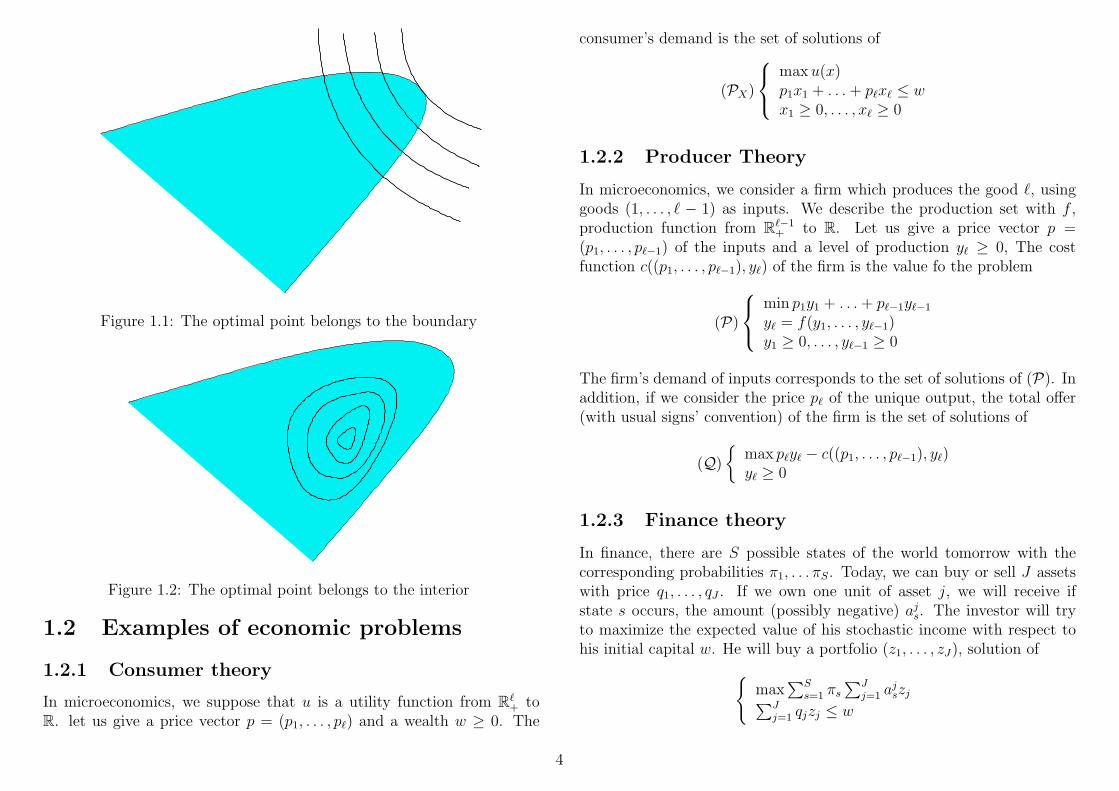
Figure 1.1: The optimal point belongs to the boundary
Figure 1.2: The optimal point belongs to the interior
1.2 Examples of economic problems
1.2.1 Consumer theory
In microeconomics, we suppose that u is a utility function from R`+ to
R. let us give a price vector p = (p1, . . . , p`) and a wealth w ≥ 0. The
consumer’s demand is the set of solutions of
(PX)
max u(x)p1x1 + . . . + p`x` ≤ wx1 ≥ 0, . . . , x` ≥ 0
1.2.2 Producer Theory
In microeconomics, we consider a firm which produces the good `, usinggoods (1, . . . , ` − 1) as inputs. We describe the production set with f ,production function from R`−1
+ to R. Let us give a price vector p =(p1, . . . , p`−1) of the inputs and a level of production y` ≥ 0, The costfunction c((p1, . . . , p`−1), y`) of the firm is the value fo the problem
(P)
min p1y1 + . . . + p`−1y`−1
y` = f(y1, . . . , y`−1)y1 ≥ 0, . . . , y`−1 ≥ 0
The firm’s demand of inputs corresponds to the set of solutions of (P). Inaddition, if we consider the price p` of the unique output, the total offer(with usual signs’ convention) of the firm is the set of solutions of
(Q)
{max p`y` − c((p1, . . . , p`−1), y`)y` ≥ 0
1.2.3 Finance theory
In finance, there are S possible states of the world tomorrow with thecorresponding probabilities π1, . . . πS. Today, we can buy or sell J assetswith price q1, . . . , qJ . If we own one unit of asset j, we will receive ifstate s occurs, the amount (possibly negative) aj
s. The investor will tryto maximize the expected value of his stochastic income with respect tohis initial capital w. He will buy a portfolio (z1, . . . , zJ), solution of{
max∑S
s=1 πs
∑Jj=1 aj
szj∑Jj=1 qjzj ≤ w
4
1.2.4 Statistics
In statistics, we determine an estimator using the maximum of the like-hood, and we determine the regression’s lines by minimizing the sum ofthe squares of the “distance to the line” among all possible lines.
1.2.5 Transportation problems
Let us consider a firm with m units of production P1, . . . , Pm, whichproduce quantities q1, . . . , qm of a certain good. There are n marketsM1, . . . ,Mn to provide whose respective demands are δ1, . . . , δn. In orderto transport one unit of good from the the unity i to the market j, there isa cost γij. We try to provide all the markets at the lowest transportationcost. We have to determine all the flows xij (quantity moved from Pi toMj) solution of
min∑m
i=1
∑nj=1 γijxij∑m
i=1 xij ≥ δj for all j,∑nj=1 xij ≤ qi for all i,
xij ≥ 0, for all i and all j
1.2.6 Constant returns to scale
Let us consider a firm using m processes P1, . . . , Pm of production. Theprocess Pj is characterized by a vector αj ∈ R`. For a single level ofactivity, there are αj
h units of good h produced by the firm if αjh ≥ 0 and
αjh units of good h used by the firm in the process if αj
h ≤ 0. The totalamount of activity of Process Pj will be denoted by xj ≥ 0.
A first class of problem consists in furnishing the demand at minimalcost. There are ` markets (one for each good) with respective demandsδ1, . . . , δn and the marginal cost of Process Pj is γj. The problem consistsin determining all activity levels xj solutions of
max∑m
j=1 γjxj∑mi=1 αj
hxj ≥ δi for all i,xj ≥ 0, for all j
A second class of problem consists in maximizing the income. We as-sume that the planer owns an initial stock σ1, . . . , σ` of inputs and that themarginal income of process j is rj. The problem consists in determiningall activity levels xj solutions of
max∑m
j=1 rjxj∑mi=1 αj
hxj ≤ σh for all h = 1, . . . , `,xj ≥ 0, for all j
5
University Paris 1 2008/2009M1–QEM1 Mr. Gourdel
Chapter 2
Convexity of sets
2.1 Definition
2.1.1 Definition of a convex set
Let E be a vector space, for all couple of elements (x, y) of E, we willdenote by [x, y], the “segment” which is the subset of E defined by
[x, y] = {tx + (1− t)y | t ∈ [0, 1]}
b
b y
x
[x, y] = [y, x]
Figure 2.1: segment
Definition 2.1 A subset C of E is convex if for all (x, y) ∈ C × C, theset [x, y] is contained in C.
Examples: For all couple of elements (x, y) in E, [x, y] is a convex subsetof E. All vector subspace is affine (see the next part), all affine subspaceis convex. All open (respectively closed) balls are convex. All set ofsolutions of linear system (involving equalities, large or strict inequalities)is convex, in particular any affine half-space. If E = R, we can characterizethe convex subsets which are the intervals.
Exercise 2.1 (*) We recall that a set J included in R is an intervall ifit satisfies the following property :
∀x ∈ J, ∀y ∈ J, ∀z ∈ R, x ≤ z ≤ y ⇒ z ∈ J.
Show that every compact interval of R is a line segment of R and thatthe only nonempty convex subsets of R are the intervals.
Exercise 2.2 (*) Use Definition 2.1 in order to show that the followingsets are convex:
a) {(x, y) ∈ R2 | x2 + y2 < 4},
b) {(x, y) ∈ R2 | |x|+ |y| ≤ 2},
c) {(x, y) ∈ R2 | max{|x|, |y|} ≤ 2},
d) the set of the (n× n)-matrices with elements ≥ 0.
Note that there is no notion of concave set. It is important toemphasize that it not a topologic concept, it can be defined even if thevector space is not embedded with a topology. Among convex sets, someof them are open, closed or even neither closed nor open.
Exercise 2.3 (**) Let A be a subset of Rn. We will introduce the fol-lowing property
Forall x ∈ A, y ∈ A, 12(x + y) ∈ A (P)
6

C
Figure 2.2: A convex and closed half space
bb
C
Figure 2.3: A convex half space which is neither closed nor open
1. Prove that this property is satisfied when A is convex.
2. Prove that Q satisfies this property though it is not a convex set.
3. We assume that A is a closed set that satisfies Property (P). Wewant to prove that it is a convex set. Let us fix x and y in A, and letus introduce the set
J = {t ∈ [0, 1], tx + (1− t)y ∈ A}.
C
Figure 2.4: A convex and open half space
a) Prove that J is a closed set containing both 0 and 1.
b) Prove that when t and t′ are in J , then (t + t′)/2 is in J .
c) Let us define for each p ∈ N, the set Jp
Jp =
{k
2p| k ∈ N, k ≤ 2p
}Prove by induction that for each p ∈ N, Jp ⊂ J . (Hint: note that(1/2)(Jp + Jp) = Jp+1.
d) Prove that J = [0, 1] and that A is convex.
4. Summarize the exercise.
Exercise 2.4 (**) In R2, consider the triangle with vertices x0, x1, x2
(non-collinear points).
1. Prove that for all u ∈ R2, there exists a unique (λ0, λ1, λ2) ∈ R3+ such
that u = λ0x0 + λ1x1 + λ2x2 and λ0 + λ1 + λ2 = 1. The coefficientsλ0, λ1, λ2 are called the barycentric coordinates of u with respect tox0, x1, x2.
2. Let y be the midpoint of the side opposite x0 and let z be the inter-section of the three medians. What are the barycentric coordinates(with respect to {x0, x1, x2}) of respectively: x0, x1, x2, y, z?
2.1.2 Definition of an affine subspace
Definition 2.2 A subset A of E is affine if for all couple of distinct pointsof A, the line defined by those two points is still in A. Formally, if for all(x, y) ∈ A× A, the set = {tx + (1− t)y | t ∈ R} is included in A.
Note that the empty set is affine. It is easy to check that any translation ofa vector subspace is an affine set. Exercise 2.8 will show that the converseis true when the set is nonempty.
Let us introduce as a complement the definition of a strictly convexset (the definition given here is not the most general).
7
Definition 2.3 Let C be a subset of E with a nonempty interior, C isstrictly convex if for all (x, y) ∈ cl C × cl C, such that x 6= y, and for allλ ∈ ]0, 1[, λx + (1− λ)y ∈ int C.
Exercise 2.5 (**) Let C be a subset contained dans E.
1. Prove that C is convex if and only if for all (x, y) ∈ C ×C, such thatx 6= y, and for all λ ∈ ]0, 1[, λx + (1− λ)y ∈ C.
2. Prove that if C is strictly convex, then C is convex.
3. If C is strictly convex and D be a subset of E such that int(C) ⊂D ⊂ cl(C), prove that D is convex.
4. Give an example of C and D, subsets of R2, such that C is convex,int(C) ⊂ D ⊂ cl(C) but D is not convex.
2.1.3 Definition of the unit simplex of Rn
Let us now introduce a very important example of convex set in Rn, theunit simplex (or “usual simplex”) denoted by Sn−1 which is defined by:
Sn−1 = {λ = (λ1, . . . , λn) ∈ Rn+ |
n∑i=1
λi = 1}
We can remark that Sn−1 is convex, closed and bounded, consequently itis a compact set.
2.2 First properties
Definition 2.4 Let (xi)ki=1, be k points of Rn. A convex combination (of
length k) of (xi)ki=1 is an element x of Rn such that there exists λ ∈ Sk−1
satisfying x =∑k
i=1 λixi.
Exercise 2.6 (*) If (x, y) is a couple of elements in Rn, show that theset of convex combinations of x and y is [x, y].
Definition 2.5 Let (xi)ni=1, be n points of Rn. An affine combination
of (xi)ni=1 is an element x of Rn such that there exists λ ∈ Rn satisfying
x =∑n
i=1 λixi and∑n
i=1 λi = 1.
Proposition 2.1 Let C be a subset of E. The set C is convex if and onlyif C contains all the convex combinations of finite families of elements ofC.
Proof of Proposition 2.1. It is obvious that if C contains all theconvex combinations of finite families of elements of C then C is a convexsubset of C.
Reciprocally, we prove the result by induction on the cardinal of thefamily. if the family has one or two elements, the definition of a convexsubset show that all convex combination of this family remain in C. Let usassume that this is true for all the families that have at most n elements.Let (x1, . . . , xn, xn+1) be a family of elements of C. Let λ ∈ Sn and letx :=
∑n+1i=1 λixi. Since
∑n+1i=1 λi = 1, there exists at least one λi which
is not equal to 0. Let us assume with no loss of generality that λ1 6= 0.Then
x =
(n∑
i=1
λi
)n∑
i=1
λin∑
i=1
λi
xi
+ λn+1xn+1
using the induction hypothesis, if we define
x′ =n∑
i=1
λin∑
i=1
λi
xi =n∑
i=1
µixi,
where µi = λin∑
i=1
λi
, we can remark that x′ is an element of C since it is a
convex combination of a family of n elements of C. In order to conclude,if we let λ =
∑ni=1 λi, λ ∈ [0, 1], this allows us to see x as a convex
8
combination of x′ and xn+1 since x = λx′ + (1− λ)xn+1. Consequently xis in C, which ends the proof. �
Proposition 2.2 Let A be a subset of E. The set A is affine if and onlyif A contains all the affine combinations of finite families of elements ofA.
Exercise 2.7 (*) Show Proposition 2.2.
Exercise 2.8 (*) Let A be a nonempty affine subset of E (vector space)and a ∈ A.
• For any a in A, let us define the translated set Ba := A − {a} =A+ {−a}. This can reformulated as, x ∈ Ba if and only if x+ a ∈ A.Check that 0 ∈ Ba.
• Deduce from Proposition 2.2 that Ba is a vector subspace of E.
• Deduce from Proposition 2.2 for if a and a are in A, then Ba = Ba,which means that the set B is independent of the particular choiceof a.
Consequently, the set B is called the direction of A and wecall affine the dimension of A the dimension of B as a vectorspace. We do not care about the dimension of the emptyset.
2.2.1 Stability by intersection
Note that the union of two convex sets is not convex.
Proposition 2.3 Let E be a vector space and let (Ci)i∈I be a family ofconvex subsets of E. Then ∩i∈ICi is convex.
Exercise 2.9 (**) Let (Ci)i∈N (respectively (Di)i) be a family of convexsubsets of some vector space E.
1) If for all integer i, Ci ⊂ Ci+1, then ∪i∈NCi is convex.
2) Show that⋃∞
k=0
⋂∞j=k Dj is a convex set.
Exercise 2.10 (**) Let (Ci)i∈I be a family of convex subsets of somevector space E.
Let us now assume that I is any set of indices and that the family ofconvex subsets satisfies that for all (i, j) ∈ I × I, there exists k ∈ I suchthat Ci ∪ Cj ⊂ Ck. then ∪i∈ICi is convex.
2.2.2 Stability by the sum operation
Proposition 2.4 Let E be a vector space. Let (Ci)i∈I , be a finite familyof convex subsets of E. Then∑
i∈I
Ci := {∑i∈I
ci | (ci) ∈∏i∈I
Ci}
is a convex subset of E.
The proof is left to the reader, it is worth to notice that for a convexset 2C = C + C and that this is not true in general.
Exercise 2.11 (**) We recall that if X is a subset of some vector spaceE, 2X = {z ∈ E | ∃x ∈ X, z = 2x}.
1. Let C be a convex subset of E. Prove that 2C = C + C.
2. Let us consider in R2, the set A = {(x, y) ∈ R2 | xy = 0}, draw A,prove that 2A = A, A + A = R2, and deduce that 2A 6= A + A.
2.3 Stability with respect to affine func-
tions
Definition 2.6 Let A and B be two affine subspace, and f : A → B.The mapping f is affine if for all couple of points (x, y) of A, and for allt ∈ R,
f(tx + (1− t)y) = tf(x) + (1− t)f(y).
Exercise 2.12 (**) Let A and B be two affine spaces with respectivedirections E and F . Let f A → B and a ∈ A.
9
1. Prove that f is an affine mapping if and only if there exists a linearmapping ϕ : E → F such that for all x of A, f(x) = f(a) + ϕ(x− a).
2. Show moreover that ϕ does not depend on the choice of a.
Consequently, ϕ is called the linear mapping associated to theaffine mapping f .
Proposition 2.5 Let E be a vector space.
(i). Let C be a convex subset of E and let α ∈ R. Then αC := {αc | c ∈C} is convex in E.
(ii). Let f , be an affine mapping from E to some affine subspace A (con-tained in some vector space F ), and let C be a convex subset of E.Then f(C) is a convex subset of F .
The proof is left to the reader.
Proposition 2.6 Let f be an affine mapping from A to B. Let us assumethat the affine subspace A is contained in the vector space E while theaffine subspace B is contained in the vector space F . Let C be a convexsubset convex of F . Then f−1(C) is a convex subset de E.
The proof is left to the reader.
Proposition 2.7 Let (Ci)i∈I be a finite family of sets such that each Ci
is a convex subset of the vector space Ei. Then∏
i∈I Ci is a convex subsetof∏
i∈I Ei.
The proof is left to the reader.
2.4 Convex hull, affine hull and conic hull
2.4.1 Convex hull and affine hull
Definition 2.7 Let A be a subset of some vector space E.
(i). The convex hull of A, denoted by co(A), is the intersection of allconvex subsets of E containing A.
(ii). The affine hull of A, denoted by Aff(A), is the intersection of all affinesubspaces of E containing A.
Remark 2.1 Note that it follows from the definition that co(∅) = ∅ andthat Aff(∅) = ∅. Since E is convex (and affine), if A is nonempty, co(A)(respectively Aff A) is well defined and nonempty. Since the set of con-vex subsets (respectively affine subsets) is stable by intersection, co(A)(respectively Aff(A)) is the smallest (in the sense of inclusion) convex (re-spectively affine) subset containing A. this implies for example that if Cis a convex subset containing A, then co(A) ⊂ C.
Proposition 2.8 Let A be a subset of some vector space E.
(i). The set co(A) is the set of all convex combinations of elementsfrom A.
(ii). The set Aff(A) is the set of all affine combinations of elementsfrom A.
Proof of Proposition 2.8. (i) Let us denote by B (respectively D), theset of all convex combinations of elements from A (respectively co(A)).One has B ⊂ D since A ⊂ (co(A)). Moreover, we can apply Proposition2.1 together with the convexity of co(A) (cf. the previous remark) in orderto get D = co(A). Consequently B ⊂ co(A).
Let us now show that co(A) ⊂ B. It is clear that A ⊂ B. Hence, inorder to prove this inclusion, il suffices to prove that B is convex. Let xand y, be two elements of B and t ∈ [0, 1]. By definition of B, there existstwo families (x1 . . . , xn) and (y1, . . . , yp) of elements from A, λ ∈ Sn−1 andµ ∈ Sp−1 such that x =
∑ni=1 λixi and y =
∑pj=1 µjyj. One has
tx + (1− t)y =n∑
i=1
tλixi +
p∑j=1
(1− t)µjyj.
10
Then tx + (1− t)y is a convex combination of (x1, . . . , xn, y1 . . . , yp) since
n∑i=1
tλi +
p∑j=1
(1− t)µj = t + (1− t) = 1
and therefore, (tλ1, . . . , tλn, (1− t)µ1 . . . , (1− t)µp) belongs to Sn+p−1.
(ii) Similar to first part. �
Definition 2.8 Let us call (convex) polytope, the convex hull of a finiteset.
Example 2.1 Let us define the simplex (denoted by Sn−1) as the subsetof Rn which is the polytope generated by the elements of the canonicbasis. The affine subspace generated by Aff(Sn−1), is the hyperplane{x ∈ Rn | x1 + . . . + xn = 1}.
Exercise 2.13 (**) Let U and V be two subsets of Rn. We will denoteby co U the closure of the convex set U .Show that: co U + co V ⊂ co(co U + V ); co U + V ⊂ co(U + V ).Prove then that co(U + V ) = co U + co V .If co U is compact, show that co(U + V ) = co U + co V .
Exercise 2.14 (*) Let A and B be convex subsetsof Rn, Let us defineD = co(A∪B) and E = {z = λx + (1− λ)y | x ∈ A, y ∈ B, 0 ≤ λ ≤ 1}.
• Show that E ⊂ D.
• Check that E is convex and contains A. Deduce that
co(A ∪B) = {z = λx + (1− λ)y | x ∈ A, y ∈ B, 0 ≤ λ ≤ 1}.
• More generally, prove that for a finite collection (Ai)pi=1 of convex
subsets of Rn,co(⋃p
i=1 Ai) = {z =∑p
i=1 λixi | λi ≥ 0, xi ∈ Ai, i =
1, . . . p,∑p
i=1 λi = 1}.
Definition 2.9 Let E be a vector space which has a finite dimension, andA be a nonempty subset, either finite or infinite. We call the dimensionof A the dimension of the affine subspace generated by A.
With this definition, it is easy to show that the unit simplex Sn−1 is(n− 1)-dimensional.
2.4.2 Cone and Conic hull
Definition 2.10 A subset K of E is a blunt cone of vertex 0 if for allx ∈ K and for all t > 0, tx belongs to K. If in addition, it contains 0, theset is a pointed cone of vertex 0.
By translation, we may define the notion of cone of vertex z.
Here, a cone will mean ici pointed cone of vertex 0.
Example, any vector subspace is a cone of vertex 0. If A is an affinesubspace and if a ∈ A, then A is a cone of vertex a. A cone can benon-convex, K = {(x, y) ∈ R2 | xy = 0}. A bounded nonempty cone isreduced to its vertex. A nonempty cone K (blunt or pointed) of vertex 0satisfies 0 ∈ ∂K.
Proposition 2.9 Let K be a subset of E.
(i). K is a pointed cone of vertex 0 if and only if for all x ∈ K and forall t ≥ 0, tx belongs to K.
(ii). A one K (pointed or blunt) is convex if and only if it is stable byaddition.
Proof of Proposition 2.9. Assertion (i) is trivial.
(ii) Let K be a convex cone. Let x an y be two elements of K. Then12(x + y) belongs to K since it is convex and x + y can be written as
2(12(x + y)) which belongs to K since it is a cone. Consequently K is
stable by addition.
Let K be a cone stable by addition and let x and y be two elementsof K. One has to show that for all t ∈ ]0, 1[, tx + (1− t)y belongs to K.
11
The vectors tx and (1− t)y are elements of K since it is a cone. Since Kis stable by addition, tx + (1− t)y belongs to K. �
Examples: All space subspace of E is a convex cone of vertex 0. Allset of solutions of a linear system of homogeneous linear equations andhomogeneous linear inequations is a convex cone. The image of a convexcone of vertex z by an affine mapping f is a convex cone which vertex isequal to f(z). The inverse image of a convex cone of vertex 0 by a linearmapping f is a convex cone which vertex is equal to 0.
Definition 2.11 Let A be a nonempty subset of E. The convex conichull of A is the intersection of all the convex pointed cone of vertex 0containing A. It is denoted by K(A).
Since E is a convex cone, the set K(A) is well defined. It is easy to provethat all intersection of convex cones is also a convex cone. Consequently,
K(A) is the smallest (in the sense of inclusion) convex cone containingA. It is also obvious that K(A) is the set of all linear combinations withnon-negative coefficients of elements from A.
12

University Paris 1 2008/2009M1–QEM1 Mr. Gourdel
Chapter 3
The one dimensional results
3.1 Existence results
The main starting point of existence results is Weierstrass’s Theorem andits corollaries.
Theorem 3.1 (Weierstrass) If the domain is compact, and if f is con-tinuous then f is bounded and the extremum are reached.
The proof is based on the notion of maximizing sequence (respectivelyminimizing). When the domain is not bounded, numerous problems canbe solved using the coercivity condition.
Definition 3.1 The function f : R → R is said coercive if
limx→−∞
f(x) = limx→+∞
f(x) = +∞.
Exercise 3.1 (*) Let us assume that f : R → R is coercive and con-tinuous, show that f has a lower bound and that there exists at least aminimum.
3.2 First order condition
3.2.1 Necessary condition
Proposition 3.1 Let −∞ ≤ a < b ≤ ∞, we let I = [a, b] ∩ R and weconsider f : I → R differentiable on I, if we assume that the problemmaxx∈I f(x) has a local solution x ∈ R, then
1. when x ∈ ]a, b[, one has f ′(x) = 0,
2. when x = a, one has f ′(x) ≤ 0,
3. when x = b, one has f ′(x) ≥ 0.
Exercise 3.2 (*) Let us use the notations of Proposition 3.1.
1. Prove Proposition 3.1.
2. Let us fix a = π. Prove that π is the solution (even it is a globalsolution) of maxx∈[π,π] e
x. What is the value of the derivative f ′(a) ?
3.2.2 Alternative formulation in terms of multipliers
Let us focus on the previous problem when the domain is bounded (a andb finite). The problem maxx∈[a,b] f(x) can be formulated as
(P)
max f(x)x− b ≤ 0a− x ≤ 0
i.e (P1)
max f(x)g1(x) ≤ 0g2(x) ≤ 0
with the notations g1(x) = x − b and g2(x) = a − x. We can stateProposition 3.1 under the following version.
13

Proposition 3.2 Let −∞ < a < b < ∞, we let I = [a, b] and we considerf : I → R differentiable on I, we assume that the problem (P1) has a localsolution x, then there exist multipliers λ1 ≥ 0 and λ2 ≥ 0 such that
f ′(x) = λ1g′1(x) + λ2g
′2(x)
and λ1g1(x) = λ2g2(x) = 0.
Exercise 3.3 (*) Deduce Proposition 3.2 from Proposition 3.1.
Be careful, if we consider the optimization problem,
(P)
{max xg1(x) = x2 ≤ 0
(3.1)
It is easy to prove that x = 0 is the unique solution of (P) but nevertherlessthe system
f ′(x) = λ1g′1(x)
λ1 ≥ 0λ1g1(x) = 0
has no solution.
Even with a single variable, the optimality does not implythe existence of multipliers, we need an additional condition(“qualification condition”). Solving the previous system dealingwith the existence of multipliers at point x makes sense only ifthis point is qualified.
We will now introduce a first version of the notion of qualification.This is not the better one, though it allow to give an intuition on thenotion.
Definition 3.2 Let us consider the following set of feasible points, theset O is open and gi are continuous on O.
x ∈ Og1(x) ≤ 0. . .gp(x) ≤ 0
We say that the Slater condition is satisfied for this list of constraints ifthere exists a point x such that x ∈ O, and for each i = 1, . . . , p,
either gi is an affine function and gi(x) ≤ 0orgi is a convex function and gi(x) < 0
Note that in the previous definition, the point x is feasible.
Exercise 3.4 (*) Let f : [a, b] → R, let us consider the optimizationproblems
(P1)
max f(x) ∈ Rx− b ≤ 0a− x ≤ 0
(P2)
max f(x)(x− b)3 ≤ 0a− x ≤ 0
1) Compare the two problems.
2) Show that the Slater condition is satisfied for (P1).
3) Show that the Slater condition is NOT satisfied for (P2).
Exercise 3.5 (*) Let us consider again the problem
(P)
{max xg1(x) = x2 ≤ 0
Show that the Slater qualification condition does not hold.
Proposition 3.3 Let x be a local solution of the optimization problem:
(P)
max f(x)x ∈ Og1(x) ≤ 0. . .gp(x) ≤ 0
Let us assume that the Slater condition is satisfied and that each functionis differentiable on a neighborhood of x, then, there exists (λi)
pi=1 ∈ Rp
+
such that {f ′(x) = λ1g
′1(x) + . . . + λpg
′p(x)
λigi(x) = 0 for all i = 1, . . . , p
14
Proof. Let us define the (possibly empty) sets, K = {i ∈ {1, . . . , p} |gi(x) = 0}, K+ = {i ∈ K | g′i(x) > 0}, K0 = {i ∈ K | g′i(x) = 0}andK− = {i ∈ K | g′i(x) < 0}. Note that we only need to prove the existenceof (λi)i∈K since when x /∈ K, the “complementary condition” λigi(x) = 0implies that λi = 0. let us prove the existence of multipliers with respectto the value of f ′(x).
If f ′(x) = 0, it suffices to let in addition λi = 0, for each i ∈ K.
Let us now consider for example the case where f ′(x) > 0, (a symmet-ric argument allows to treat the case where f ′(x) < 0). We can introducethe alternative problem
(P1)
{max f(x)gi(x) ≤ 0, for all i ∈ K
Using Exercise 1.4, we know that x is also a local solution of (P1).
Step 1 Let us prove that K+ ∪ K0 is nonempty. First, one can notice thatthere exists some ε > 0, such that for each x ∈ ]x, x + ε], gk(x) < 0,for each k ∈ K−, and f(x) > f(x). The value of ε can be chosen suchthat that x is a global solution of
(P2)
max f(x)gi(x) ≤ 0, for all i ∈ Kx ∈ [x− ε, x + ε]
Since f(x+ε) > f(x), there exists some k ∈ K such that gk(x+ε) > 0.In view of the choice of ε, we already know that k /∈ K−.
Step 2 Let us know prove that K+ is nonenmpty. If K+ is empty, then k ∈K0, and the convexity of gk implies that x is a global minimum for gk.The Slater condition assumes that either gk is affine or gk(x) < 0 =gk(x). The second case is excluded and therefore gk is affine and moreprecisely constant. This is not possible since gk(x + ε) > 0 = gk(x).
Step 3 Since K is nonempty, we can choose some k ∈ K, and let λi = 0 if i 6= k
λk =f ′(x)g′k(x)
It is obvious that (λi) satisfies all the conditions.
3.3 Convex and concave functions
3.3.1 Definitions
In this part, f is a function defined on U convex subset (interval) of R toR.
Definition 3.3 The function f is convex (resp. concave) if for all (x, y) ∈U × U and for all t ∈ [0, 1],
f(tx + (1− t)y) ≤ tf(x) + (1− t)f(y).
(respectively) f(tx + (1− t)y) ≥ tf(x) + (1− t)f(y).
The function f is strictly convex if for all (x, y) ∈ U × U such thatx 6= y and for all t ∈ ]0, 1[, f(tx + (1− t)y) < tf(x) + (1− t)f(y).
A function f is convex if and only if −f is concave. Consequently,the results obtained for convex functions can be translated in terms ofconcave functions. These notions can be defined locally.
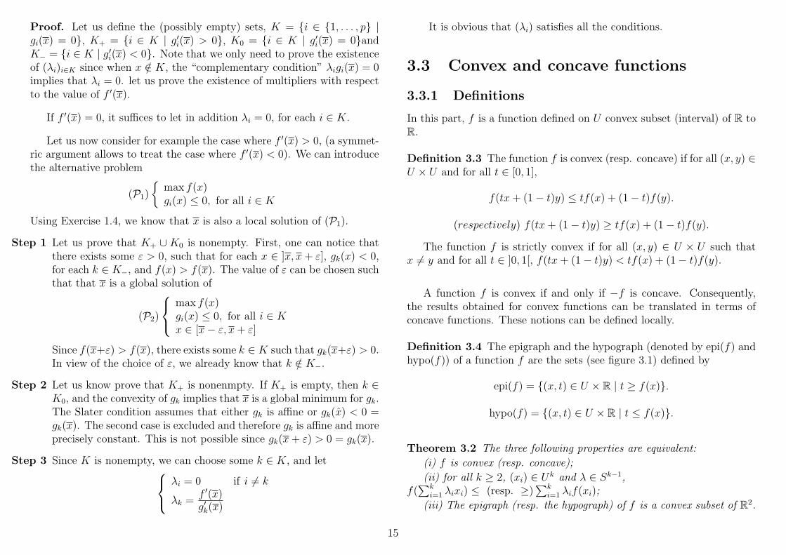
Definition 3.4 The epigraph and the hypograph (denoted by epi(f) andhypo(f)) of a function f are the sets (see figure 3.1) defined by
epi(f) = {(x, t) ∈ U × R | t ≥ f(x)}.
hypo(f) = {(x, t) ∈ U × R | t ≤ f(x)}.
Theorem 3.2 The three following properties are equivalent:
(i) f is convex (resp. concave);
(ii) for all k ≥ 2, (xi) ∈ Uk and λ ∈ Sk−1,f(∑k
i=1 λixi) ≤ (resp. ≥)∑k
i=1 λif(xi);
(iii) The epigraph (resp. the hypograph) of f is a convex subset of R2.
15

Cf
E(f)
H(f)
Figure 3.1: graph, epigraph and hypograph
Proof of Theorem 3.2. We will only prove the result in the convexcase. It is obvious that (ii) implies (i). Let us now show that (i) implies(iii). Let (x, λ) and (y, µ) two elements of epi(f) and let t ∈ [0, 1]. Itmeans that f(x) ≤ λ and f(y) ≤ µ. Since f is convex, f(tx + (1− t)y) ≤tf(x) + (1 − t)f(y). Then, f(tx + (1 − t)y) ≤ tλ + (1 − t)µ. This isequivalent to t(x, λ) + (1− t)(y, µ) = (tx + (1− t)y, tλ + (1− t)µ) belongsto the epigraph of f . Therefore, this set is convex.
We will end the proof by showing that (iii) implies (ii). Let k ≥ 2,(xi) ∈ (Rn)k and λ ∈ Sk. then, (xi, f(xi)) is an element of the epigraphof f and since this set is convex,
k∑i=1
λi(xi, f(xi)) = (k∑
i=1
λixi,k∑
i=1
λif(xi))
is an element of epi(f). Then, by definition of the epigraph,f(∑k
i=1 λixi) ≤∑k
i=1 λif(xi). �
Examples:
1. Let us recall a function R → R, is an affine function if there exists αand β such that for all x in R,
f(x) = αx + β.
Any affine function is both convex and concave, but not strictly. Itcan be easily proved that if f is convex and concave on U , then it isthe restriction on U of an affine function.
2. |.| is a convex function.
3. If C is a nonempty convex convex subset of R, the distance to Cdefined by dC(x) = inf{|x− c| such that c ∈ C} is convex.
Proposition 3.4 (i) A finite sum of convex functions (resp. concave)defined on U is convex (resp. concave);
(ii) if f is convex (resp. concave) and λ > 0, λf is convex (resp.concave);
(iii) The supremum (resp. infimum) of a family of convex functions(resp. concave) defined on U is convex (resp. concave) on its domain(when the supremum is finite);
(iv) If f is a convex function (resp. concave) from I to J , intervals ofR, and if ϕ is a convex function (resp. concave) non-decreasing from I toR then ϕ ◦ f is convex (resp. concave).
(v) if g is an affine function from R to R and f a convex function onU ⊂ R, then f ◦ g is a convex function on g−1(U).
The proof of this proposition is left to the reader.
Exercise 3.6 (*) Let f be the function defined by f(x) = −|x| on R,
Show that f is convex on [0, +∞[ and on ]−∞, 0] but not on R.
3.3.2 quasi-convex functions
Definition 3.5 Let f be a real-valued function defined on an interval I,we say that f is quasi-concave if for all α ∈ R, the set {x ∈ I | f(x) ≥ α}is convex. We say that f is quasi-convex if the sets {x ∈ I | f(x) ≤ α}are convex.
Exercise 3.7 (*) Let f be a real-valued function defined on an intervalU ,
Show that f is quasi-convex if and only if for all x, y of U and allλ ∈ [0, 1],
f(λx + (1− λ)y) ≤ max(f(x), f(y))
Proposition 3.5 Let f be a real-valued function defined on an interval,
1) if f is convex, then f is quasi-convex.
2) The function f is quasi-convex if and only if (−f) is quasi-concave.
16

3) if f is weakly monotone, then f is both quasi-concave and quasi-convex.
For example, the exponential function is convex and quasi-concave.
Exercise 3.8 (*) Show Proposition 3.5.
Exercise 3.9 (*) Let U be an open interval of R and f be a function C1
from U to R. Show that f is quasi-convex if and only if
∀x,∈ U, ∀y ∈ U, f(y) ≤ f(x) ⇒ f ′(x)(x− y) ≤ 0.
Exercise 3.10 (*) Let f be the function defined by f(x) = −|x| on R,
Show that f is quasi-convex on [0, +∞[ and on ]−∞, 0] but not on R.
There exists several notions of strict quasi-convexity, and one shouldbe cautious and check the definition used. Here we will use the followingdefinition.
Definition 3.6 Let f be a real-valued function defined on an interval U ,We say that f is strictly quasi-convex if f is quasi-convex and if for allx, y from U satisfying x 6= y and for all λ ∈ ]0, 1[,
f(λx + (1− λ)y) < max(f(x), f(y))
When the function is continuous, we can propose another characteri-zation of strict convexity (see exercise 3.11).
Exercise 3.11 (**) Let f be a continuous real-valued function definedon an interval U , we assume that for all x, y from U satisfying x 6= y,f(x) = f(y) and for all λ ∈ ]0, 1[,
f(λx + (1− λ)y) < f(x)
Show that f is strictly quasi-convex.
Exercise 3.12 (**) Let U be an open interval of R and f be a strictlyquasi-convex function:
1. Show that if x is a local solution of minx∈U f(x), then it is also aglobal solution.
2. If there exists a solution to the minimization problem, then it isunique.
Exercise 3.13 (**) Let U be an open interval of R and f a function C2
from U → R. We assume that for all x ∈ U , f ′(x) = 0 ⇒ f ′′(x) > 0.
1. The goal of this question is to show by contradiction that f is strictlyquasi-convex :
a) Let x0 6= x1 be two elements of U , such that there exists xλ ∈]x0, x1[ satisfying f(xλ) ≥ max(f(x0), f(x1)). Show that the problemmaxu∈[x0,x1] f(u) has at least one solution z satisfying z ∈ ]x0, x1[.
b) Show that f ′(z) = 0, and that f ′′(z) > 0. Deduce the contradic-tion.
2. Let x ∈ U , such that f ′(x) = 0, show that x is the unique globalminimum (necessary and sufficient condition). (Hint, one may useexercise 3.12).
3. Let g be a function U → R C1, such that g′(x) 6= 0 for all x ∈ U ,show that g is both strictly quasi-convex and strictly quasi-concave.
Exercise 3.14 1) Show with a counter-example that the sum of twoquasi-convex functions is not necessarily quasi-convex.
2) Show with a counter-example that the sum of a quasi-convex functionand a convex function is not necessarily quasi-convex.
3)Show with a counter-example that the sum of a strictly quasi-convexfunction and a strictly convex function is not necessarily quasi-convex.
3.3.3 Regularity of convex functions
We will give in this part important results on the continuity of convexfunctions.
17
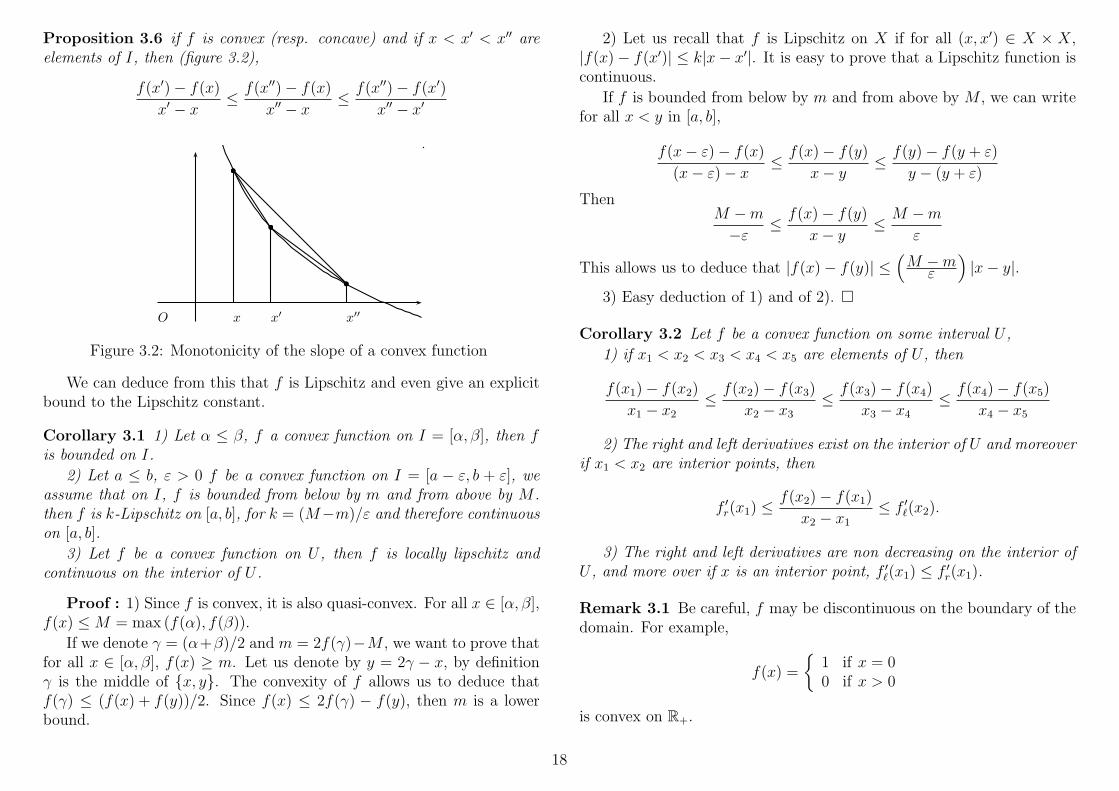
Proposition 3.6 if f is convex (resp. concave) and if x < x′ < x′′ areelements of I, then (figure 3.2),
f(x′)− f(x)
x′ − x≤ f(x′′)− f(x)
x′′ − x≤ f(x′′)− f(x′)
x′′ − x′
O
b
bb
b
b
b
.
x x′ x′′
Figure 3.2: Monotonicity of the slope of a convex function
We can deduce from this that f is Lipschitz and even give an explicitbound to the Lipschitz constant.
Corollary 3.1 1) Let α ≤ β, f a convex function on I = [α, β], then fis bounded on I.
2) Let a ≤ b, ε > 0 f be a convex function on I = [a − ε, b + ε], weassume that on I, f is bounded from below by m and from above by M .then f is k-Lipschitz on [a, b], for k = (M−m)/ε and therefore continuouson [a, b].
3) Let f be a convex function on U , then f is locally lipschitz andcontinuous on the interior of U .
Proof : 1) Since f is convex, it is also quasi-convex. For all x ∈ [α, β],f(x) ≤ M = max (f(α), f(β)).
If we denote γ = (α+β)/2 and m = 2f(γ)−M , we want to prove thatfor all x ∈ [α, β], f(x) ≥ m. Let us denote by y = 2γ − x, by definitionγ is the middle of {x, y}. The convexity of f allows us to deduce thatf(γ) ≤ (f(x) + f(y))/2. Since f(x) ≤ 2f(γ) − f(y), then m is a lowerbound.
2) Let us recall that f is Lipschitz on X if for all (x, x′) ∈ X × X,|f(x)− f(x′)| ≤ k|x− x′|. It is easy to prove that a Lipschitz function iscontinuous.
If f is bounded from below by m and from above by M , we can writefor all x < y in [a, b],
f(x− ε)− f(x)
(x− ε)− x≤ f(x)− f(y)
x− y≤ f(y)− f(y + ε)
y − (y + ε)
ThenM −m
−ε≤ f(x)− f(y)
x− y≤ M −m
ε
This allows us to deduce that |f(x)− f(y)| ≤(
M −mε
)|x− y|.
3) Easy deduction of 1) and of 2). �
Corollary 3.2 Let f be a convex function on some interval U ,
1) if x1 < x2 < x3 < x4 < x5 are elements of U , then
f(x1)− f(x2)
x1 − x2
≤ f(x2)− f(x3)
x2 − x3
≤ f(x3)− f(x4)
x3 − x4
≤ f(x4)− f(x5)
x4 − x5
2) The right and left derivatives exist on the interior of U and moreoverif x1 < x2 are interior points, then
f ′r(x1) ≤f(x2)− f(x1)
x2 − x1
≤ f ′`(x2).
3) The right and left derivatives are non decreasing on the interior ofU , and more over if x is an interior point, f ′`(x1) ≤ f ′r(x1).
Remark 3.1 Be careful, f may be discontinuous on the boundary of thedomain. For example,
f(x) =
{1 if x = 00 if x > 0
is convex on R+.
18

Exercise 3.15 (***) Let f be a function defined on some interval I, andlet x be a point of I. Let us define the set
∂f(x) = {α ∈ R | f(x) ≥ f(x) + α(x− x), for all x ∈ I}.
1. Show that if x is an interior point of I, and if the right and the lefderivatives exists at point x, then for all α ∈ ∂f(x), we have f ′r(x) ≥ αand α ≤ f ′l (x).
2. We assume that f is convex. Deduce from Proposition 3.2 that if xis an interior point of I, ∂f(x) = [f ′l (x), f ′r(x)], in particular, that theset is nonempty.
3. Let f : R → R defined by f(x) = min(0,−x), determine for all x inR, the set ∂f(x)
4. We assume that f is convex and that ∂f(x) = {a}, show that f isdifferentiable at point x and that f ′(x) = a.
3.3.4 Characterization with derivatives
Let us end this part by studying the possible characterizations when thefirst (respectively the second) derivative exists.
Proposition 3.7 Let f be a differentiable function defined on some con-vex set U ⊂ R. The function f is convex if and only if for all (x, y) ∈U × U , f(y)− f(x) ≥ f ′(x)(y − x).
Proof of Proposition 3.7. Let us first consider the implication ⇒.Let (x, y) ∈ U × U . If x = y, there is nothing to prove. Let us assumenow that x 6= y, using mean value Theorem, there exists some c in ]x, y[if x < y and in ]y, x[ if y < x such that
f(y)− f(x)
y − x= f ′(c)
The weak monotony of f ′ (See Corollary 3.2) allows us to conclude.
Conversely, we assume that the property on the derivative of f issatisfied. Let (x, y) ∈ U × U and let t ∈]0, 1[. We have
f(x)− f(x + t(y − x)) ≥ f ′(x + t(y − x))(−t(y − x))
and
f(y)− f(x + t(y − x)) ≥ f ′(x + t(y − x))((1− t)(y − x)).
If we multiply the first inequality by (1 − t), the second inequality by t,and if we sum, then we get that (1− t)(f(x)− f(x + t(y−x))) + t(f(y)−f(x + t(y− x))) ≥ (−t(1− t) + t(1− t))f ′(x + t(y− x))(y− x) = 0. Thenf(x + t(y − x)) = f((1− t)x + ty) ≤ (1− t)f(x) + tf(y), i.e. f is convex.�
The next exercise propose an alternative proof of the converse impli-cation.
Exercise 3.16 Let f be a differentiable mapping defined on the convexset U , we assume that for all (x, x′) ∈ U×U , f(x)−f(x′) ≥ f ′(x′)(x−x′).
1) Show that
epi(f) =⋂
x′∈U
{(x, y) ∈ U × R | y ≥ f(x′) + f ′(x′)(x− x′)}.
2) Using the characterization given by Theorem 3.2, deduce that f isconvex.
The monotony of f ′ characterize entirely the convexity, this can beformalized in the next proposition.
Proposition 3.8 Let f be a differentiable function on the interval U .The function f is convex if and only if for all (x, y) ∈ U × U , (f ′(y) −f ′(x))(y − x) ≥ 0.
Proof of Proposition 3.8. The implication ⇒ is a consequence of theweak monotony of f ′ (see Corollary 3.2).
For the converse implication, let us consider x and y two elements ofU . Using the proposition 3.7, it suffices to show that f(y)− f(x)− (x−
19

y)f ′(x) ≥ 0 in order to prove that f is convex. If x = y, there is nothingto prove.
We will first consider the case x > y. Since y − x < 0, we haveby assumption that for all t of ]y, x[, (f ′(t) − f ′(x))(t − x) ≥ 0, andconsequently f ′(t)− f ′(x) ≤ 0. If we integrate on [y, x] this inequality, weget
∫ x
y(f ′(t)− f ′(x))dt ≤ 0, this means f(y)− f(x)− (x− y)f ′(x) ≥ 0,
The proof of the case x < y is similar. �
Let us now consider the case where f is twice differentiable on U .
Corollary 3.3 Let f be a twice differentiable function on the interval U ,f is convex if and only if for all x ∈ U , f ′′(x) ≥ 0.
Proof of Proposition 3.3. Indeed, f is convex, if and only if f ′ isweakly increasing, therefore if and only if f ′′ ≥ 0 on U . �In order to get a result involving strict convexity, we may use the resultsof the next exercise.
Exercise 3.17 1) Show that the function f defined by f(x) = x4 isstrictly convex on R but nevertheless the second derivative is not alwayspositive on R since f ′′(0) = 0.
2) Let f be a twice differentiable function on the interval U . Show that iffor all x ∈ U , f ′′(x) > 0, then f is strictly convex on U .
3) Let f be a C2 function on U a neighborhood of x, and assume thatf ′′(x) > 0. Show that there exists V a (possibly smaller) neighborhood ofx such that f is strictly convex on V .
4) Let f be a C1 function on some interval U such that f ′ is increasing(strictly). Prove that f is strictly convex on V .
3.4 Sufficient conditions for optimality
When the problem is not convex, the only case where we can conclude isthe following:
Proposition 3.9 Let −∞ ≤ a < b ≤ ∞, we let I = [a, b] ∩ R and weconsider f : I → R differentiable at point a. If f ′(a) > 0, a is a localsolution of minimization problem.
When the problem is “convex”, we can state:
Proposition 3.10 Let us consider the optimization problem :max f(x)x ∈ Og1(x) ≤ 0. . .gp(x) ≤ 0
We assume that x is a feasible point for this system. If the function fis globally concave, (respectively locally concave at point x), and if thefunctions gi are globally convex, (respectively locally convex at point x)and if there exists (λi)
pi=1 ∈ Rp
+ such that{f ′(x) = λ1g
′1(x) + . . . + λpg
′p(x)
λigi(x) = 0 for all i = 1, . . . , p.
then, the condition is sufficient, x is a global solution (respectively local)of the maximization problem.
Proof of the proposition 3.10. Let us call the “Lagrangian” of theproblem L(x) = f(x)−
∑pi=1 λigi(x). Since this function is globally con-
cave, (respectively locally concave at point x) and L′(x) = 0, we can writethat for all point x feasible (respectively feasible and in a neighborhood ofx), L(x) ≤ L(x). we can conclude if we note that for each feasible pointx, L(x) ≥ f(x) and that L(x) = f(x) (in view of the conditions on themultipliers). �.
Exercise 3.18 Let us consider the problem:
(P)
{min x3
−1− x ≤ 0
1) Check that the Slater condition is satisfied, that the objective functionis strictly quasi-concave, that the constraint function is convexe.
2) Write the conditions for the existence of a multiplier at some feasiblepoint x and show that there exists two solutions: “x = 0 associated tothe multiplier λ = 0” and “x = −1 associated to the multiplier λ = 3”.
3) Show that the point x = 0 is not a solution (even a local solution) ofour optimization problem.
20

3.5 Introduction to sensibility analysis
Let us consider in this part an optimization problem with a single inequal-ity constraint involving one real parameter β
(Pβ)
{max f(x)g(x) ≤ β
We assume that the functions f and g are C1 on R and that for all β,there exists a unique solution xβ. We denote by ϕ(β) the value of (Pβ),we want to study the behavior of the function ϕ. Note that it is obviousthat when β increases, the set of feasible points is bigger or equal, whichimplies that the function ϕ will be non-decreasing.
Theorem 3.3 Let us assume that the function f is strictly concave, gconvex, that for all x of R, g′(x) > 0, and that the limit of f in −∞ is−∞, then for all β,
1. there exists a unique solution denoted by h(β).
2. the function h is continuous at point β and has a right and left deriva-tive at each point.
3. the function ϕ is C1 at point β and ϕ′(β) = λβ where λβ is the uniquemultiplier associated to the optimal solution h(β).
Proof of Theorem 3.3. According to the question of existence, sinceg is increasing, there exists an inverse and the problem can be equivalentlystated as maxx∈]−∞,g−1(β)] f(x). Since limx→−∞ f(x) = −∞, and since fis continuous (in view of its concavity on R), this problems has a solutionwhich is unique since f is strictly concave.
Let us first remark that the assumption on g′ implies that each pointof the domain will be qualified. Therefore x is solution of (Pβ) if and onlyif there exists a multiplier λ. Then, (x, λ) is solution of (Sβ)
(Sβ)
λ ≥ 0f ′(x) = λg′(x)λ(g(x)− β) = 0g(x)− β ≤ 0
⇔
λ = f ′(x)/g′(x) ≥ 0(f ′(x)/g′(x))(g(x)− β) = 0g(x)− β ≤ 0
⇔ (S ′β)
f ′(x) ≥ 0f ′(x)(g(x)− β) = 0g(x)− β ≤ 0
One should note that the associated multiplier is unique. In order tostudy the regularity of the value function, we will distinguish several casedepending on the sign of the multiplier.
First case: g(h(β)) < β.In this case, the associated multiplier denoted by λβ is equal to 0. Wehave, {
f ′(xβ) = 00.(g(xβ)− β) = 0
For all β′ close enough to β, g(h(β)) < β′ and the couple (h(β), 0) issolution of (Pβ′), i.e. that h(β′) = h(β). The solution is here constant.Since ϕ(β′) = f(xβ′), we can deduce that ϕ′(β) = 0 = λβ.
Second case : g(xβ) = β and λβ > 0.
We have, (S ′β)
{f ′(h(β)) > 0g(h(β))− β = 0
In view of the implicit function theorem, there exists ε > 0, and afunction γ : [β − ε, β + ε] → [h(β) − ε, h(β) + ε], such that for all β′ ∈[β − ε, β + ε], g(γ(β′)) = β′.
It is obvious that locally γ(β′) is solution of (S ′β′), this means thatlocally h = γ, in particular h is C1 in a neighborhood of β. Since ϕ(β′) =f(h(β′)), we can deduce that
ϕ′(β) = γ′(β)f ′(γ(β)) =1
g′(h(β))f ′(h(β)) = λβ
Third case : g(xβ) = β and λβ = 0.We have, {
f ′(xβ) = 0g(xβ)− β = 0
• As in the first case, for all β′ > β and close enough to β, the couple(h(β), 0) is solution of (Pβ′), i.e. that h(β′) = h(β). We can deduce
21
that h is continuous on the right, has a right derivative, at point β,moreover the right derivative ϕ′r(β) = 0 = λβ.
• As in the second case, for all β′ < β close enough to β, in view ofthe implicit function theorem, there exists ε > 0, and a functionγ : [β−ε, β +ε] → [xβ−ε, xβ +ε], such that for all β′ ∈ [β−ε, β +ε],g(γ(β′)) = β′.
It remains to study the sign of the multiplier. Since f ′(γ(β)) = 0,γ is increasing, we can deduce that the strict concavity of f impliesthat f ′(γ(β′)) ≥ 0 for all β′ < β close enough to β. Then γ(β′) issolution of (S ′β′), i.e. h = γ. We can deduce that h is continuous onthe left, has a left derivative at point β, moreover the left derivative
ϕ′`(β) = γ′(β)f ′(γ(β)) =1
g′(xβ)f ′(xβ) = λβ
In this theorem, h is not necessarily C1, while ϕ = f ◦ h is C1. �.
Exercise 3.19 Let β be a real parameter, we consider the problem
(Pβ)
{max−x2
x ≤ β
Show thatSol(Pβ) = {0} if β ≥ 0 and {β} if β ≤ 0
Deduce that in particular the solution is not differentiable at point 0 withrespect to β.
Exercise 3.20 Let h defined by h(x) = g(−x).
1) Compare the sets of solutions and the values of the problems
(Pβ)
{max f(x)g(x) ≤ β
(Qβ)
{max f(−x)h(x) ≤ β
2) Deduce, that in Theorem 3.3, the conclusion remains true if we replacethe condition “for all x, g′(x) > 0” by “for all x, g′(x) < 0”.
22

University Paris 1 2008/2009M1–QEM1 Mr. Gourdel
Chapter 4
Finite dimensional optimization
4.1 Existence results
As in dimension 1, the main starting point of existence results is Weier-strass’s Theorem and its corollaries.
Theorem 4.1 (Weierstrass) Let f be a function whose domain is com-pact, and if f is continuous then f is bounded and the extrema are reached.
The proof uses the notion of maximizing sequence (cf. Definition 1.5)and is based on the following lemma.
Lemma 4.1 Let us consider a maximizing sequence (xk)k. If the domainis closed, the objective function f is continuous, then any cluster point of(xk)k is a solution to the maximization problem.
When the domain is not bounded, numerous problems can be solvedusing the coercivity condition.
Definition 4.1 The function f : A → R is said coercive if
lim‖x‖→+∞
f(x) = +∞.
Proposition 4.1 Let us assume that f : A → R is coercive and contin-uous, and that A is closed, then f has a lower bound and there exists atleast a minimum.
Exercise 4.1 (*) Let us consider the following optimization problem.
(P)
min x + ys.t. x ≥ 0
y ≥ 0(1 + x)(1 + y) ≤ 2
1. Draw the set of feasible points compact.
2. Prove that we can apply 4.1 to this problem.
Exercise 4.2 (*) Let us consider the following optimization problem.
(P)
max 3x1x2 − x3
2
s.t. x1 ≥ 0x2 ≥ 0x1 − 2x2 = 52x1 + 5x2 ≥ 20
1. Is the set of feasible points compact ?
2. Prove that we can apply Proposition 4.1 to the “modified” problem
(Q)
min −3x1x2 + x3
2
s.t. x1 ≥ 0x2 ≥ 0x1 − 2x2 = 52x1 + 5x2 ≥ 20
3. conclude
23

4.2 Convex and quasi-convex functions
4.2.1 Definitions
In this part, f is a function defined on U convex subset of Rn with valuesin R.
Definition 4.2 The function f is convex (resp. concave) if for all (x, y) ∈U × U and for all t ∈ [0, 1],
f(tx + (1− t)y) ≤ tf(x) + (1− t)f(y).
(respectively) f(tx + (1− t)y) ≥ tf(x) + (1− t)f(y).
The function f is strictly convex if for all (x, y) ∈ U × U such thatx 6= y and for all t ∈ ]0, 1[, f(tx + (1− t)y) < tf(x) + (1− t)f(y).
Exercise 4.3 (**)
1. Let U be an open convex set on which the function f is assumed tobe convex, We assume moreover that f is continuous on the closureof U . Show that f is convex on U .
2. Let U = R2++ = {x ∈ R2 | x1 > 0 and x2 > 0}, let us consider f
defined on U by f(x1, x2) = 4√
x1x2). Is f strictly concave on U? onU?
A function f is convex if and only if −f is concave. Consequently,the results obtained for convex functions can be translated in terms ofconcave functions. These notions can be defined locally.
Definition 4.3 Let f be a real-valued function defined on a convex setU , we say that f is quasi-concave if for all α ∈ R, the set {x ∈ U | f(x) ≥α} is convex. We say that f is quasi-convex if for all α ∈ R, the set{x ∈ U | f(x) ≤ α} is convex.
There exist several notions of strict quasi-convexity, and one shouldbe cautious and check the definition used. Here we will use the followingdefinition.
Definition 4.4 Let f be a real-valued function defined on a convex setU , We say that f is strictly quasi-convex if f is quasi-convex and if for allx, y from U satisfying x 6= y and for all λ ∈ ]0, 1[,
f(λx + (1− λ)y) < max(f(x), f(y))
Exercise 4.4 (**)
1. Let U be an open convex set on which the function f is assumed tobe quasi-convex, We assume moreover that f is continuous on theclosure of U . Show that f is quasi-convex on U .
2. Let U = R2++ = {x ∈ R2 | x1 > 0 and x2 > 0}, let us consider f
defined on U by f(x1, x2) = 4√
x1x2). Is f strictly quasi-concave onU? on U?
Remark 4.1 Let U be a convex subset of Rn. One has the equivalence
• The function f is convex (respectively strictly convex, quasi-convex,strictly quasi convex) on U ,
• for all x 6= y in U , the function ϕx,y defined from [0, 1] to R by,
ϕx,y(t) = f(ty + (1− t)x) = f(x + t(y − x))
is convex (respectively strictly convex, quasi-convex, strictly quasiconvex) on [0, 1].
Note that ϕx,y is differentiable (resp. twice differentiable) when f is differ-entiable (resp. twice differentiable) then, ϕ′x,y(t) = 〈∇f(x+t(y−x)), y−x〉and ϕ′′x,y(t) = 〈Hf (x + t(y − x)))(y − x), y − x〉.
Definition 4.5 The epigraph and the hypograph (denoted by epi(f) andhypo(f)) of a real-valued function f are the sets (see figure 4.1) definedby
epi(f) = {(x, t) ∈ U × R | t ≥ f(x)}.
hypo(f) = {(x, t) ∈ U × R | t ≤ f(x)}.
24

��� ������
Figure 4.1: graph and epigraph
Theorem 4.2 The three following properties are equivalent:
1. f is convex (resp. concave);
2. for all k ≥ 2, (xi) ∈ Uk and λ ∈ Sk−1, (unit simplex of Rk)f(∑k
i=1 λixi) ≤ (resp. ≥)∑k
i=1 λif(xi);
3. The epigraph (resp. the hypograph) of f is a convex subset of Rn+1.
Proof of Theorem 4.2. Simple adaptation of the proof of Theorem 3.2
Examples:
1. Any affine real-valued function is both convex and concave, but notstrictly. It can be easily proved that if f is convex and concave on U ,then it is the restriction to U of an affine function, (still called affinefunction by an abuse of language).
2. Each norm is a convex function.
3. If C is a nonempty convex subset of Rn, the distance to C defined bydC(x) = inf{‖x− c‖ such that c ∈ C} is convex.
Proposition 4.2 1. A finite sum of convex functions (resp. concave)defined on U is convex (resp. concave);
2. if f is convex (resp. concave) and λ > 0, λf is convex (resp. con-cave);
3. The supremum (resp. infimum) of a family of convex functions (resp.concave) defined on U is convex (resp. concave) on its domain (whenthe supremum is finite);
4. If f is a convex function (resp. concave) from U (convex set of Rn)to I (interval of R), and if ϕ is a convex function (resp. concave)non-decreasing from I to R then ϕ ◦ f is convex (resp. concave) onU .
5. if g is an affine function from Rn to Rp and f a convex function onU ⊂ Rp, then f ◦ g is a convex function on g−1(U).
The proof of this proposition is left to the reader.
Exercise 4.5 Let U be a convex set of Rn and f be a convex function:
Show that if x is a local solution of minx∈U f(x), then it is also a globalsolution.
Exercise 4.6 (*) Let f be a real-valued function defined on a convexset U , show that f is quasi-convex if and only if for all x, y of U and allλ ∈ [0, 1],
f(λx + (1− λ)y) ≤ max(f(x), f(y))
Exercise 4.7 (*) Let U be an open convex set of Rn and f be a strictlyquasi-convex function:
1. Show that if x is a local solution of minx∈U f(x), then it is also aglobal solution.
2. If there exists a solution to the minimization problem, then it isunique.
When the function is regular, we can propose characterizations of(strict) quasi-convexity (see exercises 4.8 and 4.9).
Exercise 4.8 (*) Let U be an open set of Rn and f be a function C1 onU . Show that f is quasi-convex if and only if
∀x,∈ U, ∀y ∈ U, f(y) ≤ f(x) ⇒ 〈∇f(x), x− y〉 ≤ 0.
25
Exercise 4.9 (*) Let f be a continuous real-valued function defined on aconvex set U , we assume that for all x, y of U satisfying x 6= y, f(x) = f(y)and for all λ ∈ ]0, 1[,
f(λx + (1− λ)y) < f(x)
Show that f is strictly quasi-convex.
Exercise 4.10 (*) Let U be a convex subset of Rn and f be a quasi-convex function. We want to study minx∈U f(x).
1. Show that the set of solution to the minimization problem is convex.
2. Prove with a counter-example that a local solution is not necessarilya global solution. Hint: consider f : R → R, defined by
f(x) =
−x− 1 if x ≤ −1,0 if x ∈ [−1, 1],x− 1 if x ≥ 1.
Exercise 4.11 (**) Let U be an open convex set of Rn and f a functionC2 from U → R. We assume that for all x ∈ U , and all v ∈ Rn \ {0},〈∇f(x), v〉 = 0 ⇒ vtHf (x)v > 0. Show that f is strictly quasi-convex.
Hint: use Exercise 3.13 and Remark 4.1.
4.2.2 Regularity of convex functions
We will give in this part important results on the continuity of convexfunctions.
Proposition 4.3 Let U be a convex set, ε > 0 and f be a convex functionon V = U + B(0, ε),
1. We assume that on V , f is bounded from below by m and from aboveby M . then f is k-Lipschitz on U , for k = (M −m)/ε and thereforecontinuous on U .
2. Let f be a convex function on U , then f is locally lipschitz and con-tinuous on the interior of U .
Note that this property is false in an infinite dimension setting. Forexample, if we consider E = R[X] (polynomial functions), embedded withthe norm
‖P‖ =
deg(P )∑k=0
|ak|, when P =
deg(P )∑k=0
akXk.
It is easy to see that the linear ϕ(and consequently convex) is NOT con-tinuous, where ϕ(P ) = P ′(0).
4.2.3 Characterization of convexity with derivatives
Let us end this part by studying the possible characterizations when thefirst (respectively the second) derivative exists.
Proposition 4.4 Let f be a differentiable function defined on some con-vex set U ⊂ Rn. The function f is convex if and only if for all(x, y) ∈ U × U ,
f(y) ≥ f(x) + 〈∇f(x), y − x〉.
Proof of Proposition 4.4.
Let us first consider the implication ⇒. Let (x, y) ∈ U ×U and x 6= y.In view of Remark 4.1, we know that the function ϕx,y is convex. Since thisfunction has a derivative, we know that ϕx,y(1)−ϕx,y(0) ≥ ϕ′x,y(0)(1− 0)which leads to the conclusion.
Conversely, we assume that the property on the gradient of f is sat-isfied. Let x0 6= x1 in U , let us consider the function ϕx0,x1 . In view ofProposition 3.7, it suffices to prove that for all t 6= t′ (in [0, 1]),
ϕx0,x1(t′)− ϕx0,x1(t) ≥ ϕ′x0,x1
(t)(t′ − t)
in order to prove that ϕx0,x1 is convex. If we denote by x = tx1 +(1− t)x0
and y = t′x1 + (1 − t′)x0, the left side of the previous inequality can beinterpreted as f(y)− f(x), while the right side is equal to 〈∇f(x), y− x〉.Since ϕx0,x1 is convex, it follows from Remark 4.1 that f is convex. �
The next exercise propose an alternative proof of the converse impli-cation.
26
Exercise 4.12 (**) Let f be a differentiable mapping defined on theconvex set U , we assume that for all (x, x′) ∈ U × U , f(x) − f(x′) ≥〈∇f(x′), x− x′〉.
1. Show that
epi(f) =⋂
x′∈U
{(x, y) ∈ U × R | y ≥ f(x′) + 〈∇f(x′), x− x′〉}.
2. Using the characterization given by Theorem 4.2, deduce that f isconvex.
Exercise 4.13 (***) Let f be a function defined on some convex set U ,and let x be an interior point. Let us define the set (cf. Exercise 3.15)
∂f(x) = {α ∈ Rn | f(x) ≥ f(x) + 〈α, x− x〉, for all x ∈ U}
In order to simplify the notations, it may be easier to consider the casex = 0.
1. Apply Proposition 4.4 in order to show that if f is convex and differ-entiable at point x, then ∇f(x) ∈ ∂f(x).
2. If f is differentiable at point x, write the Taylor expansion of degree1 at a neighborhood of x, and deduce that α ∈ ∂f(x) ⇒ α = ∇f(x).
3. We assume that f is convex and that ∂f(x) = {α}, show that f isdifferentiable at point x and that ∇f(x) = α.
Proposition 4.5 Let f be a differentiable function on some convex setU . The function f is convex if and only if for all (x, y) ∈ U × U ,
〈∇f(y)−∇f(x), y − x〉 ≥ 0.
Proof of Proposition 4.5. The implication ⇒ is a consequence ofRemark 4.1. Indeed, we know that the function ϕx,y is convex, whichimplies ϕ′x,y(1)− ϕ′x,y(0) ≥ 0. This leads to the conclusion.
For the converse implication, let us consider x and y two elements ofU . We know that for all t of ]0, 1[,
〈∇f(ty + (1− t)x)−∇f(x), (ty + (1− t)x)− x〉 ≥ 0,
and consequently 〈∇f(ty + (1 − t)x), y − x〉 ≥ 〈∇f(x), y − x〉. If weintegrate on [0, 1] this inequality, we get∫ 1
0
(〈∇f(ty + (1− t)x), y − x〉dt ≥ 〈∇f(x), y − x〉,
this means f(y) − f(x) − 〈∇f(x), x − y〉 ≥ 0. Using Proposition 4.4, wecan deduce that f is convex. �
Let us now consider the case where f is twice differentiable on U . Wewill denote by Hf (x) the hessian matrix at point x, we recall that thismatrix is symmetric when f is C2.
Definition 4.6 Let M be a symmetric matrix (n, n).
• We say that M is positive semidefinite (respectively negative semidef-inite) if for all v ∈ Rn, 〈v, Mv〉 ≥ 0 (respectively 〈v, Mv〉 ≤ 0).
• We say that M is positive definite (respectively negative definite) iffor all v ∈ Rn \ {0}, 〈v, Mv〉 > 0 (respectively 〈v, Mv〉 < 0).
Proposition 4.6 Let M be a symmetric matrix (n, n).
• the matrix M has n eigenvalues (possibly equal),
• the matrix M is positive semidefinite (respectively negative semidef-inite) if and only if all eigenvalues are non-negative, (respectivelynon-positive),
• the matrix M is positive definite (respectively negative definite) if andonly if all eigenvalues are positive, (respectively negative).
Exercise 4.14 (*) Let M be a symmetric (n, n)−matrix, then
• if M is positive semidefinite, then det M ≥ 0 and Tr(M) ≥ 0.
27
• if M is positive definite, then det M > 0 and Tr(M) > 0.
• if M is negative semidefinite, then Tr(M) ≤ 0 and det M ≤ 0 whenn is odd, det M ≥ 0 when n is even.
• if M is negative definite, then Tr(M) < 0 and det M < 0 when n isodd, det M > 0 when n is even.
Exercise 4.15 (*) When the dimension is equal to 2, we can reenforce
the conclusion of the previous exercise. Let M =
(r ss t
)be a symmetric
(2, 2)−matrix, then
• the matrix M is positive semidefinite if and only if det M ≥ 0 andTr(M) ≥ 0.
• the matrix M is positive definite if and only if det M > 0 andTr(M) > 0.
Exercise 4.16 (*) Let M be the following matrix,
M =
−1 0 00 −1 00 0 3
Show that det M > 0 and Tr(M) > 0, and that M is not positive semidef-inite.
Proposition 4.7 Let M be a symmetric matrix, then M is positive defi-nite if and only if for all k = 1, . . . , n, ∆k > 0, where
∆k =
∣∣∣∣∣∣∣a11 . . . a1k...
. . ....
ak1 . . . akk
∣∣∣∣∣∣∣Exercise 4.17 (*) 1) Let M be a symmetric matrix, such that M ispositive semidefinite, then for all k = 1, . . . , n, ∆k ≥ 0, where
∆k =
∣∣∣∣∣∣∣a11 . . . a1k...
. . ....
ak1 . . . akk
∣∣∣∣∣∣∣
2) Let M be the following matrix,
M =
3 0 00 0 00 0 −1
Prove that for all k = 1, . . . , 3, ∆k ≥ 0, but that M is not positivesemidefinite.
Proposition 4.8 Let f be a twice continuously differentiable function onU , which is a convex and open subset of Rn. Then, f is convex if andonly if for all x ∈ U , Hf (x) is positive semidefinite.
Proof of Proposition 4.8. Indeed, if f is convex, then for any xin U and v in Rn, there exists ε > 0, such that y = x + εv ∈ U . Wecan consider the function ϕx,y which is convex. We can deduce that〈εv, Hf (x)εv〉ϕ′′x,y(0) ≥ 0. This implies that Hf (x) is positive semidefi-nite.
Conversely, let us assume that at each point of U , Hf (x) is positivesemidefinite. Then the computation of ϕ′′x,y (cf. Remark 4.1) allows us todeduce that ϕx,y is convex. �
A simple adaptation of the previous proof allows us to deduce thefollowing proposition:
Proposition 4.9 Let f be a twice continuously differentiable function onsome convex set U ,
1) If for all x ∈ U , Hf (x) is positive definite, then f is strictly convex.
2) If at point x, the hessian matrix is positive definite, then f is strictlyconvex in some neighborhood of x.
4.3 Unconstrained optimization
4.3.1 Classical case
The problem maxx∈U f(x) is said unconstrained if the set U is an opensubset of Rn.
28
Remark 4.2 Let us consider the unconstrained problem minx∈U f(x) andx ∈ U . The point x is a local solution of this problem if and only if it isan interior point of the set {x ∈ U | f(x) ≥ f(x)}.
Remark 4.3 The previous remark can only be used for unconstrainedoptmization: for example, x = (0, 0) is a local solution of the problemminx∈U f(x) (where U = R2
+ NOT open and f(x) = x21 + x2
2), but thecorresponding set {x ∈ U | f(x) ≥ f(x)} is reduced to {x} and theinteriory property does not hold.
Proposition 4.10 Let us consider the unconstrained problemminx∈U f(x).
• If x is a local solution, and if f is differentiable at point x, then∇f(x) = 0, (“critical point”)
• If x is a local solution, and if f is twice continuously differentiable atpoint x, then Hf (x) is positive semidefinite,
• If x is a critical point, if f is twice continuously differentiable atpoint x, and if Hf (x) is positive definite, then x is a local solution.In addition, there exists some ε > 0, such that on B(x, ε) ⊂ U , x isthe unique solution.
• If x is a critical point and if f is convex, then x is a global solution.
Proof of Proposition 4.10
It suffices to remark that if x is a local solution, then for any directionu ∈ Rn, there exists some positive real number ε > 0, such that thefunction
ϕ : ]−ε, ε[ → Rϕ(t) = f(x + tu)
is defined, and that 0 is a (global) minimum.
If f is differentiable at point x, then ϕ has a derivative and ϕ′(0) = 0.In view of the chain rule theorem, ϕ′(t) = 〈∇f(x + tu), u〉. This leads to〈∇f(x), u〉 ≥ 0. Since this is true for any u ∈ Rn, we can conclude that∇f(x) = 0.
If f is twice differentiable at point x, then ϕ has a second derivative andϕ′′(0) ≥ 0. In view of the chain rule theorem, ϕ′′(t) = 〈u, Hf (x + tu)(u)〉.This leads to 〈u, Hf (x)(u)〉 = 0. Since this is true for any u ∈ Rn, we canconclude that Hf (x) is positive semidefinite.
Note that some results of unconstrained optimization can be used evenif the domain is not open (cf. Exercise 1.5).
Remark 4.4 Let x is a local solution of the problem minx∈X f(x). WhenX is a neighborhood of x, there exists some V open subset of C containingx such that x is a local solution of the problem minx∈V f(x). This allowsto apply the first and second order necessary conditions.
Exercise 4.18 We can reenforce the third result of the previous proposi-tion. For all k strictly smaller than the smallest eigenvalue of the Hessianmatrix Hf (x) (in particular, k can be chosen positive), there exists someε > 0 such that for all x ∈ B(x, r), f(x) ≥ f(x) + k
2‖x− x‖2.
4.3.2 Extension to affine constraints
Let us consider the following problem{min f(x)x ∈ U,Ax = b
The set of feasible points C is {x ∈ U | Ax = b}, where A is a (n× p)-matrix and b ∈ Rp. This correspond to the case of p affine constraintsrepresented by the p rows of A and the vector b. If we denote by aj thevector de Rn corresponding to the j-row of A, the set C is defined by:
x ∈ C if and only if 〈aj, x〉 − bj = 0 for all j = 1, . . . , p.
If we denote by gj(x) = 〈aj, x〉 − bj (which are affine functions), andJ = {1, . . . , p}, the problem can be written as
min f(x)gj(x) = 0, ∀j ∈ Jx ∈ U
29
Note that C can be written as U∩Λ−1(b) where Λ is the linear mappingdefined by x → Λ(x) = Ax. Let x be a local solution of the problem:
min f(x)Ax = bx ∈ U
For all u ∈ Ker Λ, note that for all t ∈ R, A(x + tu) = b.
Since U is open et x ∈ U , there exists some ε > 0 such that for allt ∈ ]−ε, ε[, x + tu ∈ U . Once again, we can consider
ϕu : ]−ε, ε[ → Rϕu(t) = f(x + tu)
Consequently, for all t ∈ ]−ε, ε[, ϕu(t) := f(x+tu) ≥ ϕu(0) = f(x), whichmeans that 0 is a minimum de ϕu. This implies that ϕ′u(0) = 0. We cancompute ϕ′u(0) = ∇f(x) · u = 0.
Let (u1, . . . uk) be a basis of the kernel
Note that when U is equal to Rn, we can entirely describe C which isequal to {x}+ Ker Λ. This implies that 0 is a solution of{
min f(x + λ1u1 + . . . + λkuk)λ1 ∈ R, . . . , λk ∈ R
In the general case, C is equal to U ∩ ({x}+Ker Λ). This implies thatthere exists ε > 0, such that 0 is a solution of
min h(λ)λ1 ∈ R, . . . , λk ∈ Rλ ∈ B(0, ε)
where h(λ) = f(x + λ1u1 + . . . + λkuk).
This leads to ∇h(0) = 0, and we can formulate this result as ∇f(x)is orthogonal to Ker Λ. It follows that ∇f(x) is in the image of Λt, thetransposed of de ϕ. We recall that the matrix of Λt is the matrix wherethe rows are the columns of A, the vectors aj. We have the result, thereexists some vector λ in Rp (vector of Lagrange multipliers) such that:
∇f(x) =
p∑j=1
λjaj
Since aj = ∇gj(x), this means that
∇f(x) =
p∑j=1
λj∇gj(x)
4.4 Karush-Kuhn-Tucker
4.4.1 Necessary condition
Let us consider the domain defined by the list of constraintsfi(x) = 0, ∀i ∈ Igj(x) ≤ 0, ∀j ∈ Jx ∈ U
Among the inequality constraints, we will distinguish those that corre-spond to affine function. This can be formulated as J is equal to thepartition Ja∪Jna, where gj is affine when j ∈ Ja. The set U is open whichmay hide strict inequalities.
Definition 4.7 We say that the Slater condition is satisfied if
• all fi are affine,
• all gj are convex
• there exists x be a feasible point of the previous system, satisfyingmoreover gj(x) < 0, for all j ∈ Jna.
Remark 4.5 When all the constraints are affine, then the Slater’s con-dition is equivalent to to the existence of a feasible point.
Theorem 4.3 (Karush-Kuhn-Tucker) Let us consider the optimiza-tion problem:
min f(x)fi(x) = 0, ∀i ∈ Igj(x) ≤ 0, ∀j ∈ Jx ∈ U
30
where U is an open set. Let x be a local solution of this problem. Weassume that there exists V open neighborhood of x such that f , fi, gj arecontinuously differentiable on V . If the Slater condition is satisfied thenthere exists λ ∈ RI and µ ∈ RJ
+ such that
∇f(x) +∑i∈I
λi∇fi(x) +∑j∈J
µj∇gj(x) = 0 (4.1)
and µjgj(x) = 0, for all j ∈ J .
Note that if we distinguish among the inequalities, the set of bindingconstraints at point x by J(x) = {j ∈ J | gj(x)}, then the condition 4.1can be rewritten as,
∇f(x) +∑i∈I
λi∇fi(x) +∑
j∈J(x)
µj∇gj(x) = 0. (4.2)
Note that when j /∈ J(x), in view of the “complementary condition”(µjgj(x) = 0), we can deduce that the multiplier µj is equal to zero.
Definition 4.8 We will associate to the previous minimization problem,the following system “Karush-Kuhn-Tucker conditions”
fi(x) = 0, ∀i ∈ Igj(x) ≤ 0, ∀j ∈ J
λi ∈ R, ∀i ∈ Iµj ≥ 0, ∀j ∈ Jµjgj(x) = 0, for all j ∈ J
∇f(x) +∑
i∈I λi∇fi(x) +∑
j∈J µj∇gj(x) = 0
x ∈ U
Exercise 4.19 1. Prove that for all z ∈ R2,
z1 ≥ 0,z2 ≥ 0,z1 + z2 = 0,
⇔{
z1 = 0,z2 = 0.
2. Prove that for any p ≥ 1, for any α ∈ Rp+, β ∈ Rp
+,
p∑i=1
αiβi = 0 ⇔ αiβi = 0, for all i = 1, . . . , p
3. Prove that the Karush-Kuhn-Tucker system is equivalent to thereexists (x, λ, µ) ∈ U × RI × RJ
+ such thatfi(x) = 0, ∀i ∈ Igj(x) ≤ 0, ∀j ∈ J∑
j∈J µjgj(x) = 0,
∇f(x) +∑
i∈I λi∇fi(x) +∑
j∈J µj∇gj(x) = 0
4.4.2 Sufficient conditions for optimality
Definition 4.9 We say that the problem
min f(x)x ∈ U ,h1(x) = 0. . .hq(x) = 0g1(x) ≤ 0. . .gp(x) ≤ 0
is convex if the functions hj are affine, the functions gi are convex, and iff is convex 1.
When the problem is convex, we can state:
Proposition 4.11 Let us consider the optimization problem:min f(x)g1(x) ≤ 0. . .gp(x) ≤ 0x ∈ U
1for a maximization problem, the objective function is concave.
31

Let us assume that x be a feasible point and that U is an open set.If the function f is convex on U (globally convex), (respectively locallyconvex at point x), and if the functions gi are convex on U , (respectivelylocally convex at point x) and if there exists (λi)
pi=1 ∈ Rp
+ such that{∇f(x) + λ1∇g1(x) + . . . + λp∇gp(x) = 0
λigi(x) = 0 for all i = 1, . . . , p.
then, the condition is sufficient, x is a global solution (respectively local)of the minimization problem.
Proof of the proposition 4.11. In order to simplify the notation, wewill focus on the global case. Let us call the “Lagrangian” of the problem
L(x, λ) = f(x) +
p∑i=1
λigi(x).
We can consider the partial function H(x) = L(x, λ), The function His convex on U , and x is a critical point of H. So for each x ∈ U (feasibleor not), H(x) ≤ H(x).
We can conclude, if in addition we notice that for each feasible pointx, gi(x) ≤ 0 ⇒ λigi(x) ≤ 0 ⇒ L(x, λ) ≤ f(x) and that L(x, λ) = f(x) (inview of the complementary relations). �
Corollary 4.1 Let us consider the optimization problem:min f(x)x ∈ Ufi(x) = 0, i ∈ Igj(x) ≤ 0, j ∈ J
Let us assume that x be a feasible point and that U is an open set. If thefunction f is (respectively locally at point x) convex, the functions fi areaffine, if for all j ∈ J(x) functions gj are convex on U (respectively locally
at point x), and if there exists (λ) ∈ RI and µ ∈ RJ(x)+ such that{
∇f(x)−∑
i∈I λi∇fi(x) +∑
j∈J(x) µj∇gj(x) = 0
µjgj(x) = 0 for all j ∈ J.
then, the condition is sufficient, (respectively sufficient) x is a solution(repectively local solution) of the minimization problem.
We can extend in the next exercise Corollary 4.1 by assuming thatthe objective function is only quasi-concave but only if the point is not acritical point (cf. Exercise 3.18).
Exercise 4.20 Let us consider (x, λ, µ) solution of Karush-Kuhn-Tuckersystem (Definition 4.8) associated to the minimization problem
min f(x)fi(x) = 0, ∀i ∈ Igj(x) ≤ 0, ∀j ∈ Jx ∈ U
We assume in addition that the objective function is quasi-concave onU and continuous on U , the functions fi are affine, and for all j ∈ J ,the functions gj are convex on U , The goal of the exercise is to show bycontradiction that if ∇f(x) 6= 0, then x is a solution of the minimizationproblem. With no loss of generality, we may assume that x = 0.
1. Let us assume that there exists some feasible point y such that f(y) <f(0), prove the existence of some ε > 0 such that for all z ∈ B(y, ε),f(z) < f(x).
2. Let us fix some z ∈ B(y, ε). Show that the function ϕ := ϕ0,z isquasi-concave and consequently ϕ′(0) ≤ 0.
3. Deduce from ∇f(x) +∑
i∈I λi∇fi(x) +∑
j∈J(x) µj∇gj(x) = 0 that
ϕ′(0) ≥ 0.
4. Compute ϕ′(0) and deduce that ∇f(0) ⊥ B(y, ε). Conclude.
4.5 Polarity and orthogonality
4.5.1 Separation theorems
Theorem 4.4 Let A and B be two nonempty disjoint convex subsets ofRn. If A is compact and B is closed, then there exists y ∈ E, y 6= 0 such
32
that:sup{y · a | a ∈ A} < inf{y · b | b ∈ B}
Theorem 4.5 Let A and B be two nonempty disjoint convex subsets ofRn. Then there exists a hyperplane separating A and B.
y ∈ E, y 6= 0 such that
sup{y · a | a ∈ A} ≤ inf{y · b | b ∈ B}
4.5.2 definitions
Definition 4.10 Let A be a subset of Rn, the polar cone of A, denotedby A◦ is defined by
A◦ = {y ∈ E | for all a ∈ A, y · a ≤ 0}
The orthogonal of A, denoted by A⊥ is defined by
A⊥ = {y ∈ E | for all a ∈ A, y · a = 0}
Proposition 4.12 Let A be a subset of Rn
1. A◦ is a closed convex cone (of vertex 0),
2. A⊥ is a linear subspace,
3. A⊥ = A◦ ∩ (−A)◦;
4. If A1 ⊂ A2, then A◦2 ⊂ A◦
1 and A⊥2 ⊂ A⊥
1 ;
5. If A 6= ∅, A◦ = (cl(K(A)))◦ and A⊥ = (vect(A))⊥ where vect(A) isthe linear subspace spanned by A.
Exercise 4.21 (*) Prove Proposition 4.12.
Exercise 4.22 Let A be a nonempty subset of Rn
1. A ⊂ A◦◦ := (A◦)◦
2. A◦ = A◦◦◦ := ((A◦)◦)◦
3. A◦◦ = A◦◦◦◦ := (((A◦)◦)◦)◦
Exercise 4.23 Let A be a nonempty subset of Rn
1. If A is a cone subspace, then y belongs to A◦ if and only if a → y · ais bounded from above on A.
2. If A is a linear subspace, then A◦ = A⊥; y belongs to A⊥ if and onlyif a → y · a is bounded from above on A. A vector y belongs to A⊥
if and only if a → y · a is bounded from below on A.
Theorem 4.6 (Bipolar Theorem) If A be a nonempty subset of Rn,then, (A◦)◦ = cl(K(A)) and (A⊥)⊥ = vect(A), where vect(A) is the linearsubspace spanned by A.
Corollary 4.2 Let A be a nonempty subset of Rn. The set A is a closedconvex cone if and only if A = (A◦)◦. The set A is a linear subspace ifand only if A = (A⊥)⊥.
Corollary 4.3 Let M be a linear subspace of Rn, M = E if and only ifM⊥ = {0}.
Exercise 4.24 Let M be a convex set of Rn. M is a neighborhood of 0if and only if M◦ = {0}.
4.5.3 Farkas’ lemma
Theorem 4.7 (Farkas’ lemma) Let (ai)i∈I be a finite family of ele-ments in Rn. Let
A = {∑i∈I
λiai | λ ∈ RI+}
and
B = {y ∈ E | y · ai ≤ 0, for all i ∈ I}
one has A◦ = B and B◦ = A.
The key argument is Exercise 4.26.
33
Exercise 4.25 (**) Let (a1, . . . , ap) be a finite subset of E = Rn.
1) Show that co(a1, . . . , ap) is a compact set.
2) Extend this result if E is a normed vector space.
Exercise 4.26 (***) Let (a1, . . . , ap) be a finite subset of E = Rn.
The goal of this exercise is to show by induction on p that the setK(a1, . . . , ap) which denotes {
∑pi=1 λiai | λ ∈ Rp
+} is closed.
A) 1) show that if −ap+1 ∈ K(a1, . . . , ap) then
K(a1, . . . , ap+1) =
p+1⋃i=1
K({aj | j 6= i}).
2) show that if M and N are two closed convex cones of E, such thatM ∩ (−N) = {0} then M + N is closed.
B) 1) Show that the result is true when p = 1.
2) Write the proof (one will have to distinguish wether −ap+1 belongsor not to K(a1, . . . , ap)).
Corollary 4.4 (Second version of Farkas’ lemma) Let (ai)i∈I and(bj)j∈J be finite families of elements in Rn. Let
A = {∑i∈I
λiai +∑j∈J
µjbj | λ ∈ RI+, µ ∈ RJ}
et
B = {y ∈ E | y · ai ≤ 0, for all i ∈ I, y · bj = 0, for all j ∈ J}
one has A◦ = B and B◦ = A.
Corollary 4.5 Let (ai)i∈I be a finite family of elements in Rn. Let
A = {∑i∈I
λiai | λ ∈ RI}
andB = {y ∈ E | y · ai = 0, pour tout i ∈ I}
One has, A⊥ = B and B⊥ = A.
Exercise 4.27 Let (ai)i=1,...,p be a finite family of elements in Rn. Letb ∈ Rn satisfying the following property:
For all y ∈ Rn y · a1 ≤ 0. . .y · ap ≤ 0
⇒ y · b ≤ 0.
Prove (using the hint) that there exists λ ∈ RI+ such that b =
∑i∈I λiai.
Hint: Prove that 0 is a solution of the following optimization problemand write the Karush-Kuhn-Tucker conditions.
max y · b y · a1 ≤ 0. . .y · ap ≤ 0
4.6 Tangent and normal cones
Let us now introduce two definitions.
Definition 4.11 Let C be a convex set containing c. The tangent coneto the set C at point c denoted by TC(c) is
TC(c) = cl{t(c′ − c) | t ≥ 0, c′ ∈ C}
The normal cone to the set C at point c denoted by NC(c) is:
NC(c) = {y ∈ E | y · c ≥ y · c′ ∀c′ ∈ C}.
Exercise 4.28 (*) (i) Let C be a convex set containing c, and D denotesis translation D := C + {−c}. Show that TC(c) = TD(0) and NC(c) =ND(0).
(ii) Let c ∈ A ⊂ B, then TA(c) ⊂ TB(c) and NB(c) ⊂ NA(c).
Proposition 4.13 (i) For all c ∈ C, TC(c) and NC(c) are nonempty,closed and convex cones.
(ii) TC(c) = (NC(c))◦ and NC(c) = (TC(c))◦.
It is very important to emphasize that these notions are local notions,cf. next exercise.
34

Exercise 4.29 (*) Let C1 and C2 be convex sets containing c, if thereexists ε > 0 such that C1 ∩ B(c, ε) = C2 ∩ B(c, ε) then NC1(c) = NC2(c)and TC1(c) = TC2(c).
Exercise 4.30 (*) Let us consider min x2 +y2 under the constraint 2x+y ≤ −4.
1) Is the Slater condition satisfied for this problem ?
2) Write the Karush-Kuhn-Tucker conditions of this problem.
3) Solve the Karush-Kuhn-Tucker system.
4) Discuss wether the conditions are necessary/sufficient in order tosolve the optimization problem.
Exercise 4.31 (**)
let us consider the following optimization problems:
(P)
max 3x1x2 − x3
2
s.c. x1 ≥ 0x2 ≥ 0x1 − 2x2 = 52x1 + 5x2 ≥ 20
(Q)
max 3x1x2 − x3
2
s.c. x1 > 0x2 > 0x1 − 2x2 = 520− 2x1 − 5x2 ≤ 0
1) Draw the set of feasible points for (P) and comment.
2) Prove that x is feasible for (P) if and only if x is feasible for (Q).Deduce that the two problems are equivalent.
3) Prove that Sol(P) is nonempty.
4) Write the Karush-Kuhn-Tucker conditions.
5) Solve the Karush-Kun-Tucker conditions.
6) Solve the optimization problem (P)
35
University Paris 1 2008/2009M1–QEM1 Mr. Gourdel
Chapter 5
Linear Programming
A linear programming problem consists in finding the maximum (resp.minimum) value of a linear functional, subject to a finite number of linearconstraints. If c and ai, i = 1, . . . ,m are elements of Rn, and if b =(b1, . . . , bm) belongs to Rm, the most general form of a linear programmingproblem is the following:
Maximize (resp. minimize)
f(x) = c · x
subject to the conditions
ai · x
≤=≥
bi, i = 1, . . . ,m
x ∈ Rn.
The linear functional f(x) is called the objective function. The linearequations and inequations are called constraints of the problem. Theset of points that satisfy these linear equations or inequations is calledfeasible set. An element of this set is a feasible solution; it is an optimalsolution if it solves the maximization (resp. minimization) problem. Let(P ) and (P ′) be two optimization problems, we recall that (P ) and (P ′)are equivalent if their sets of solutions are equal.
Note that in general, we can not use Weierstrass theorem neither acoercivity property of the objective function.
5.1 The main results
5.1.1 existence
Note that in general, we can not use Weierstrass theorem neither a coer-civity property of the objective function.
Proposition 5.1 Given a linear programming problem (P ) (maximiza-tion), one of the three following alternatives holds:
- either there is no feasible point for Problem (P ), the value is equalto −∞, Sol(P ) = ∅.
- either the objective function is not bounded from above on thenonempty set of feasible points, the value is equal to +∞, Sol(P ) = ∅.
- either the objective function is not bounded from above on thenonempty set of feasible points, the value is finite and the set of solutionsis nonempty.
5.1.2 Necessary and sufficient conditions of optimal-ity
Let fk (resp. f ′k) k = 1, . . . , q, hk (resp. h′k) k = 1, . . . , r, g (resp.g′) be linear functional on Rn, αk (resp. α′k) k = 1, . . . , q, βk (resp.β′k) k = 1, . . . , r be real numbers. We now consider linear programming
36
problems expressed in the following form:
(I)
Minimize g(x) subject tofk(x) = αk, k = 1, . . . , qhk(x) ≥ βk, k = 1, . . . , rx ∈ Rn.
Proposition 5.2 For a feasible solution x to be an optimal solution ofProblem (I), it is both necessary and sufficient that there exist some KKTmultipliers µ1, . . . , µq ∈ R and ν1, . . . , νr ∈ R+.
Note that the Slater condition is satisfied if and only if there exists afeasible point.
Corollary 5.1 For a feasible solution x to be an optimal solution of Prob-lem (I), it is both necessary and sufficient that there exist µ1, . . . , µq ∈ Rand ν1, . . . , νr ∈ R+ such that g =
∑qk=1 µkf
k +∑r
k=1 νkhk, with νk = 0 if
hk(x) > βk.
5.2 Saddle point properties
(P )min f(x) subject to
fi(x) ≤ 0, i ∈ Ix ∈ Rn.
The Lagrangian of minimization Problem (P ) is the function L : Rn ×RI
+ → R defined by for all (x, λ) = (x, (λi)i∈I),
L(x, λ) = f(x) +∑i∈I
λifi(x).
We say that (x, λ) is a saddle-point of L if for all ∀λ ∈ RI+,∀x ∈ Rn,
L(x, λ) ≥ L(x, λ) ≥ L(x, λ).
Theorem 5.1 (i) If (x, λ) is a saddle-point of L, then x is a solution to(P ) and (λ) are the Karush-Kuhn-Tucker coefficients associated with x.Moreover, L(x, λ) = f(x).(ii) If (x, λ) satisfies Karush-Kuhn-Tucker Conditions for Problem (P ),then (x, λ) is a saddle-point of L.
In this case, the dual problem can be defined as
(D)max G(λ) subject to
λ ∈ RI+.
where
G(λ) = infx∈Rn
L(x, λ)
Note that G(λ) = L(x, λ) = f(x) = val(P )
5.3 The duality theorem of linear program-
ming
5.3.1 Canonical form of the duality theorem
Let A be a (m×n)-matrix, b ∈ Rm, c ∈ Rn. Let us consider the followinglinear programming problem (P ), here referred to as the primal problem,
(P )
Minimize c · x subject toAx ≥ bx ≥ 0x ∈ Rn.
and define its dual problem (D)
(D)
Maximize b · p subject totpA ≤ tcp ≥ 0p ∈ Rm.
37
Writing down the dual of the dual leads to the given primal problem.For this reason, the linear programming problems (P ) and (D) are referredto as primal problem and dual problem in canonical form. Each one of bothproblems is said to be the dual of the other one.
Proposition 5.3 Given the pair of dual linear programming problems(P ) and (D), one of the two following alternatives holds:
- either (P ) and (D) have a couple (x, p) of optimal solutions satisfy-ing: p · b = c · x (obviously, the same relation p · b = c · x holds then forevery couple (x, p) of optimal solutions since the primal and the dual havethe same value);
- or neither (P ) nor (D) has an optimal solution and one of bothfeasible sets is empty.
In what follows, the duality theorem is used to establish an importantresult on linear inequalities which extends Exercise4.27.
5.3.2 Application to nonhomogeneous Farkas’lemma
Exercise 5.1 (***) Let for every i = 0, 1, . . . ,m, ai ∈ Rn, αi ∈ R besuch that the system ai ·x ≤ αi, i = 1, . . . ,m is consistent. Then in orderthat the following implication is true
ai · x ≤ αi, i = 1, . . . ,m ⇒ a0 · x ≤ α0 (5.1)
it is necessary and sufficient that there exist nonnegative real numbersλi ≥ 0 such that
a0 =m∑
i=1
λiai and α0 ≥
m∑i=1
λiαi.
Exercise 5.2 Let p1 > 0, p2 > 0 and the optimization problem
(P)
min −x1 − x2
s.c. x1 ≥ 0, x2 ≥ 0p1x1 + p2x2 ≤ 1
1) Write the Karush-Kuhn-Tucker conditions of (P), solve the primal.
2) Write the dual and solve it.
38
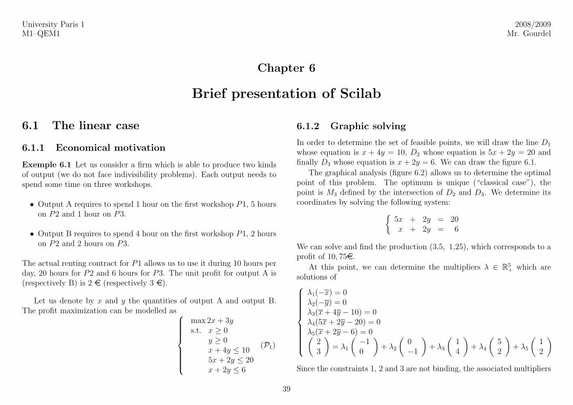
University Paris 1 2008/2009M1–QEM1 Mr. Gourdel
Chapter 6
Brief presentation of Scilab
6.1 The linear case
6.1.1 Economical motivation
Exemple 6.1 Let us consider a firm which is able to produce two kindsof output (we do not face indivisibility problems). Each output needs tospend some time on three workshops.
• Output A requires to spend 1 hour on the first workshop P1, 5 hourson P2 and 1 hour on P3.
• Output B requires to spend 4 hour on the first workshop P1, 2 hourson P2 and 2 hours on P3.
The actual renting contract for P1 allows us to use it during 10 hours perday, 20 hours for P2 and 6 hours for P3. The unit profit for output A is(respectively B) is 2 e (respectively 3 e).
Let us denote by x and y the quantities of output A and output B.The profit maximization can be modelled as
max 2x + 3ys.t. x ≥ 0
y ≥ 0x + 4y ≤ 105x + 2y ≤ 20x + 2y ≤ 6
(P1)
6.1.2 Graphic solving
In order to determine the set of feasible points, we will draw the line D1
whose equation is x + 4y = 10, D2 whose equation is 5x + 2y = 20 andfinally D3 whose equation is x + 2y = 6. We can draw the figure 6.1.
The graphical analysis (figure 6.2) allows us to determine the optimalpoint of this problem. The optimum is unique (“classical case”), thepoint is M3 defined by the intersection of D2 and D3. We determine itscoordinates by solving the following system:{
5x + 2y = 20x + 2y = 6
We can solve and find the production (3,5, 1,25), which corresponds to aprofit of 10, 75e.
At this point, we can determine the multipliers λ ∈ R5+ which are
solutions of
λ1(−x) = 0λ2(−y) = 0λ3(x + 4y − 10) = 0λ4(5x + 2y − 20) = 0λ5(x + 2y − 6) = 0(
23
)= λ1
(−10
)+ λ2
(0−1
)+ λ3
(14
)+ λ4
(52
)+ λ5
(12
)Since the constraints 1, 2 and 3 are not binding, the associated multipliers
39
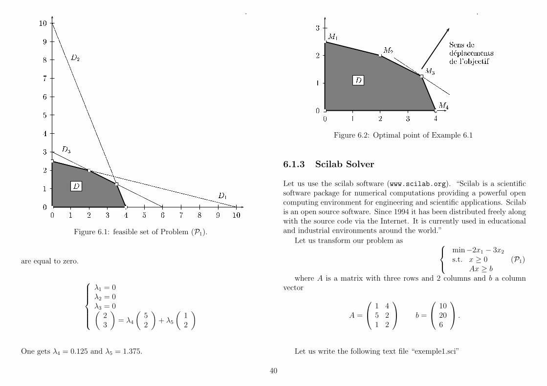
� � � � � � � � � ���
�
�
�
�
�
�
�
�
��
��������
��������
��������
�����
�����������������������������
�� ����
����
��������
��
����
���
���
Figure 6.1: feasible set of Problem (P1).
are equal to zero.
λ1 = 0λ2 = 0λ3 = 0(
23
)= λ4
(52
)+ λ5
(12
)
One gets λ4 = 0.125 and λ5 = 1.375.
� � � � ��
�
�
�
� � � � �
�����
������ �� ��������������������� ������! #"%$&�����')(
*+ *+,-
,-./
./01
0123
23
4
576
598
5;:
59<
Figure 6.2: Optimal point of Example 6.1
6.1.3 Scilab Solver
Let us use the scilab software (www.scilab.org). “Scilab is a scientificsoftware package for numerical computations providing a powerful opencomputing environment for engineering and scientific applications. Scilabis an open source software. Since 1994 it has been distributed freely alongwith the source code via the Internet. It is currently used in educationaland industrial environments around the world.”
Let us transform our problem as min−2x1 − 3x2
s.t. x ≥ 0Ax ≥ b
(P1)
where A is a matrix with three rows and 2 columns and b a columnvector
A =
1 45 21 2
b =
10206
.
Let us write the following text file “exemple1.sci”
40
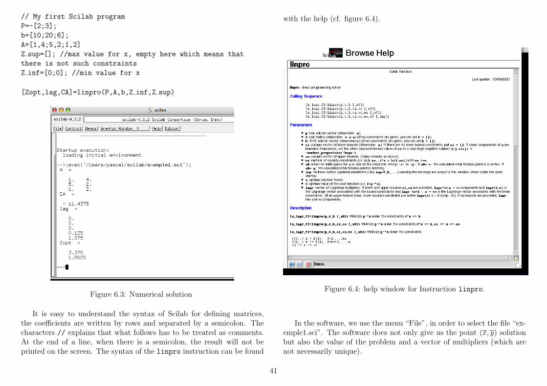
// My first Scilab program
P=-[2;3];
b=[10;20;6];
A=[1,4;5,2;1,2]
Z sup=[]; //max value for x, empty here which means that
there is not such constraints
Z inf=[0;0]; //min value for x
[Zopt,lag,CA]=linpro(P,A,b,Z inf,Z sup)
Figure 6.3: Numerical solution
It is easy to understand the syntax of Scilab for defining matrices,the coefficients are written by rows and separated by a semicolon. Thecharacters // explains that what follows has to be treated as comments.At the end of a line, when there is a semicolon, the result will not beprinted on the screen. The syntax of the linpro instruction can be found
with the help (cf. figure 6.4).
Figure 6.4: help window for Instruction linpro.
In the software, we use the menu “File”, in order to select the file “ex-emple1.sci”. The software does not only give us the point (x, y) solutionbut also the value of the problem and a vector of multipliers (which arenot necessarily unique).
41
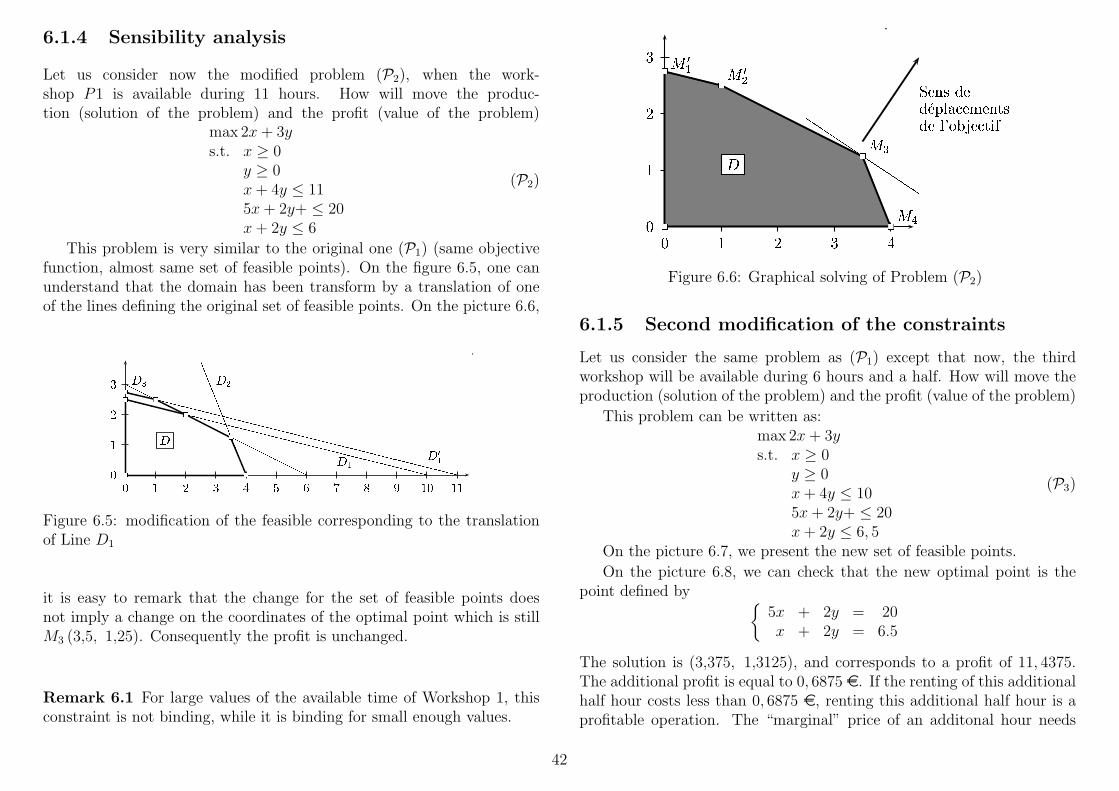
6.1.4 Sensibility analysis
Let us consider now the modified problem (P2), when the work-shop P1 is available during 11 hours. How will move the produc-tion (solution of the problem) and the profit (value of the problem)
max 2x + 3ys.t. x ≥ 0
y ≥ 0x + 4y ≤ 115x + 2y+ ≤ 20x + 2y ≤ 6
(P2)
This problem is very similar to the original one (P1) (same objectivefunction, almost same set of feasible points). On the figure 6.5, one canunderstand that the domain has been transform by a translation of oneof the lines defining the original set of feasible points. On the picture 6.6,
� � � � � � � � � �� ����
�
�
�
��������
��������
��������
�����
��������
��������
��������
��������
����
����
����
����
��
�� ����
��������
�� ���� ������
��
���� �! �
�#"�%$
Figure 6.5: modification of the feasible corresponding to the translationof Line D1
it is easy to remark that the change for the set of feasible points doesnot imply a change on the coordinates of the optimal point which is stillM3 (3,5, 1,25). Consequently the profit is unchanged.
Remark 6.1 For large values of the available time of Workshop 1, thisconstraint is not binding, while it is binding for small enough values.
� � � � ��
�
�
�
� � � � �
�����
������ �� �������������������� ���� �"!$#&%'���)(+*
,- ,-./
./01
01232345
45
6
798: 7 8;
7=<
7?>
Figure 6.6: Graphical solving of Problem (P2)
6.1.5 Second modification of the constraints
Let us consider the same problem as (P1) except that now, the thirdworkshop will be available during 6 hours and a half. How will move theproduction (solution of the problem) and the profit (value of the problem)
This problem can be written as:max 2x + 3ys.t. x ≥ 0
y ≥ 0x + 4y ≤ 105x + 2y+ ≤ 20x + 2y ≤ 6, 5
(P3)
On the picture 6.7, we present the new set of feasible points.
On the picture 6.8, we can check that the new optimal point is thepoint defined by {
5x + 2y = 20x + 2y = 6.5
The solution is (3,375, 1,3125), and corresponds to a profit of 11, 4375.The additional profit is equal to 0, 6875 e. If the renting of this additionalhalf hour costs less than 0, 6875 e, renting this additional half hour is aprofitable operation. The “marginal” price of an additonal hour needs
42
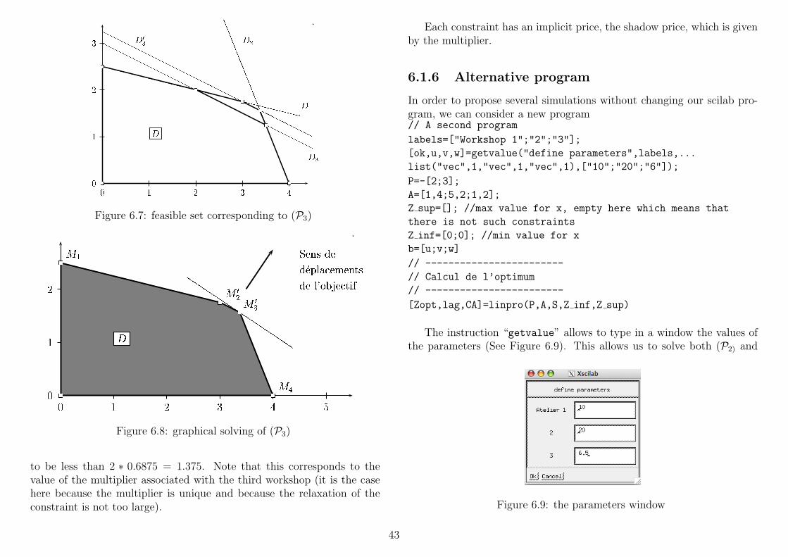
� � � � ��
�
�
�
� � � � � � � � � � � � � � � � � � � � � � � � � � �
����������������������
� � � � � � � � � � � � � � � � � � � � � � � � � � � � �
� � � � � � � � � � � � � � � � � � � � � � � � � � � � �
� ��
��
� ��
��
����
����
��
��
��
��
�
���
�������
� �
Figure 6.7: feasible set corresponding to (P3)
� � � � � ��
�
�
� � � � � �
������
��� ��� ������� ����������������� ��� �"!$#&%'������(*)
+, +,-.
-./0/012
1234
34
5
687
6:9; 6:9<
6>=
Figure 6.8: graphical solving of (P3)
to be less than 2 ∗ 0.6875 = 1.375. Note that this corresponds to thevalue of the multiplier associated with the third workshop (it is the casehere because the multiplier is unique and because the relaxation of theconstraint is not too large).
Each constraint has an implicit price, the shadow price, which is givenby the multiplier.
6.1.6 Alternative program
In order to propose several simulations without changing our scilab pro-gram, we can consider a new program// A second program
labels=["Workshop 1";"2";"3"];
[ok,u,v,w]=getvalue("define parameters",labels,...
list("vec",1,"vec",1,"vec",1),["10";"20";"6"]);
P=-[2;3];
A=[1,4;5,2;1,2];
Z sup=[]; //max value for x, empty here which means that
there is not such constraints
Z inf=[0;0]; //min value for x
b=[u;v;w]
// ------------------------
// Calcul de l’optimum
// ------------------------
[Zopt,lag,CA]=linpro(P,A,S,Z inf,Z sup)
The instruction “getvalue” allows to type in a window the values ofthe parameters (See Figure 6.9). This allows us to solve both (P2) and
Figure 6.9: the parameters window
43
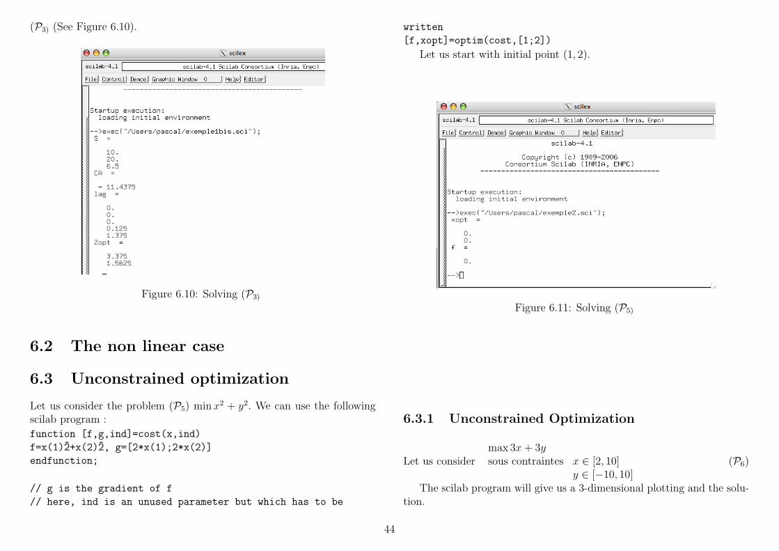
(P3) (See Figure 6.10).
Figure 6.10: Solving (P3)
6.2 The non linear case
6.3 Unconstrained optimization
Let us consider the problem (P5) min x2 + y2. We can use the followingscilab program :
function [f,g,ind]=cost(x,ind)
f=x(1)2+x(2)2, g=[2*x(1);2*x(2)]
endfunction;
// g is the gradient of f
// here, ind is an unused parameter but which has to be
written
[f,xopt]=optim(cost,[1;2])
Let us start with initial point (1, 2).
Figure 6.11: Solving (P5)
6.3.1 Unconstrained Optimization
Let us considermax 3x + 3ysous contraintes x ∈ [2, 10]
y ∈ [−10, 10](P6)
The scilab program will give us a 3-dimensional plotting and the solu-tion.
44
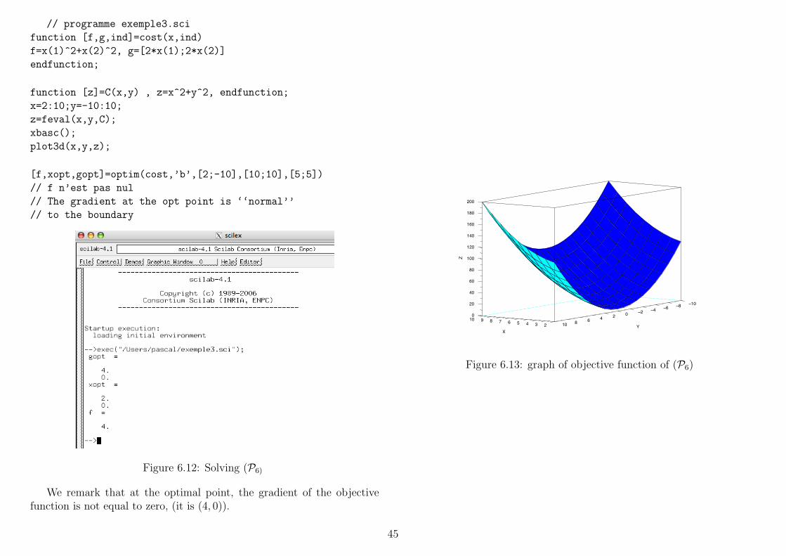
// programme exemple3.sci
function [f,g,ind]=cost(x,ind)
f=x(1)^2+x(2)^2, g=[2*x(1);2*x(2)]
endfunction;
function [z]=C(x,y) , z=x^2+y^2, endfunction;
x=2:10;y=-10:10;
z=feval(x,y,C);
xbasc();
plot3d(x,y,z);
[f,xopt,gopt]=optim(cost,’b’,[2;-10],[10;10],[5;5])
// f n’est pas nul
// The gradient at the opt point is ‘‘normal’’
// to the boundary
Figure 6.12: Solving (P6)
We remark that at the optimal point, the gradient of the objectivefunction is not equal to zero, (it is (4, 0)).
0
20
40
60
80
100
120
140
160
180
200
Z
!10!8!6!4!20246810 Y2345678910
X
Figure 6.13: graph of objective function of (P6)
45
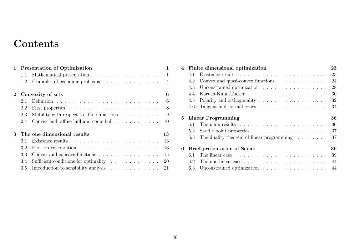
Contents
1 Presentation of Optimization 1
1.1 Mathematical presentation . . . . . . . . . . . . . . . . . . 1
1.2 Examples of economic problems . . . . . . . . . . . . . . . 4
2 Convexity of sets 6
2.1 Definition . . . . . . . . . . . . . . . . . . . . . . . . . . . 6
2.2 First properties . . . . . . . . . . . . . . . . . . . . . . . . 8
2.3 Stability with respect to affine functions . . . . . . . . . . 9
2.4 Convex hull, affine hull and conic hull . . . . . . . . . . . . 10
3 The one dimensional results 13
3.1 Existence results . . . . . . . . . . . . . . . . . . . . . . . 13
3.2 First order condition . . . . . . . . . . . . . . . . . . . . . 13
3.3 Convex and concave functions . . . . . . . . . . . . . . . . 15
3.4 Sufficient conditions for optimality . . . . . . . . . . . . . 20
3.5 Introduction to sensibility analysis . . . . . . . . . . . . . 21
4 Finite dimensional optimization 23
4.1 Existence results . . . . . . . . . . . . . . . . . . . . . . . 23
4.2 Convex and quasi-convex functions . . . . . . . . . . . . . 24
4.3 Unconstrained optimization . . . . . . . . . . . . . . . . . 28
4.4 Karush-Kuhn-Tucker . . . . . . . . . . . . . . . . . . . . . 30
4.5 Polarity and orthogonality . . . . . . . . . . . . . . . . . . 32
4.6 Tangent and normal cones . . . . . . . . . . . . . . . . . . 34
5 Linear Programming 36
5.1 The main results . . . . . . . . . . . . . . . . . . . . . . . 36
5.2 Saddle point properties . . . . . . . . . . . . . . . . . . . . 37
5.3 The duality theorem of linear programming . . . . . . . . 37
6 Brief presentation of Scilab 39
6.1 The linear case . . . . . . . . . . . . . . . . . . . . . . . . 39
6.2 The non linear case . . . . . . . . . . . . . . . . . . . . . . 44
6.3 Unconstrained optimization . . . . . . . . . . . . . . . . . 44
46