Introduction to KerasTensorFlow

Marco Rorrom.rorro@cineca.it

CINECA – SCAI SuperComputing Applications and Innovation Department

1/33

Table of Contents

Introduction

Keras

Distributed Deep Learning

2/33

Introduction

Keras

Distributed Deep Learning

3/33

TensorFlow

I Google Brain’s second generation machine learning system

I computations are expressed as stateful data-flow graphsI automatic differentiation capabilitiesI optimization algorithms: gradient and proximal gradient basedI code portability (CPUs, GPUs, on desktop, server, or mobile computing platforms)I Python interface is the preferred one (Java, C and Go also exist)I installation through: pip, Docker, Anaconda, from sourcesI Apache 2.0 open-source license

4/33

TensorFlow

I Google Brain’s second generation machine learning systemI computations are expressed as stateful data-flow graphs

I automatic differentiation capabilitiesI optimization algorithms: gradient and proximal gradient basedI code portability (CPUs, GPUs, on desktop, server, or mobile computing platforms)I Python interface is the preferred one (Java, C and Go also exist)I installation through: pip, Docker, Anaconda, from sourcesI Apache 2.0 open-source license

4/33

TensorFlow

I Google Brain’s second generation machine learning systemI computations are expressed as stateful data-flow graphsI automatic differentiation capabilities

I optimization algorithms: gradient and proximal gradient basedI code portability (CPUs, GPUs, on desktop, server, or mobile computing platforms)I Python interface is the preferred one (Java, C and Go also exist)I installation through: pip, Docker, Anaconda, from sourcesI Apache 2.0 open-source license

4/33

TensorFlow

I Google Brain’s second generation machine learning systemI computations are expressed as stateful data-flow graphsI automatic differentiation capabilitiesI optimization algorithms: gradient and proximal gradient based

I code portability (CPUs, GPUs, on desktop, server, or mobile computing platforms)I Python interface is the preferred one (Java, C and Go also exist)I installation through: pip, Docker, Anaconda, from sourcesI Apache 2.0 open-source license

4/33

TensorFlow

I Google Brain’s second generation machine learning systemI computations are expressed as stateful data-flow graphsI automatic differentiation capabilitiesI optimization algorithms: gradient and proximal gradient basedI code portability (CPUs, GPUs, on desktop, server, or mobile computing platforms)

I Python interface is the preferred one (Java, C and Go also exist)I installation through: pip, Docker, Anaconda, from sourcesI Apache 2.0 open-source license

4/33

TensorFlow

I Google Brain’s second generation machine learning systemI computations are expressed as stateful data-flow graphsI automatic differentiation capabilitiesI optimization algorithms: gradient and proximal gradient basedI code portability (CPUs, GPUs, on desktop, server, or mobile computing platforms)I Python interface is the preferred one (Java, C and Go also exist)

I installation through: pip, Docker, Anaconda, from sourcesI Apache 2.0 open-source license

4/33

TensorFlow

I Google Brain’s second generation machine learning systemI computations are expressed as stateful data-flow graphsI automatic differentiation capabilitiesI optimization algorithms: gradient and proximal gradient basedI code portability (CPUs, GPUs, on desktop, server, or mobile computing platforms)I Python interface is the preferred one (Java, C and Go also exist)I installation through: pip, Docker, Anaconda, from sources

I Apache 2.0 open-source license

4/33

TensorFlow

I Google Brain’s second generation machine learning systemI computations are expressed as stateful data-flow graphsI automatic differentiation capabilitiesI optimization algorithms: gradient and proximal gradient basedI code portability (CPUs, GPUs, on desktop, server, or mobile computing platforms)I Python interface is the preferred one (Java, C and Go also exist)I installation through: pip, Docker, Anaconda, from sourcesI Apache 2.0 open-source license

4/33

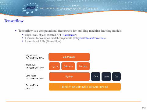
Tensorflow

I Tensorflow is a computational framework for building machine learning modelsI High-level, object-oriented API (tf.estimator)I Libraries for common model components (tf.layers/tf.losses/tf.metrics)I Lower-level APIs (TensorFlow)

5/33

Introduction

Keras

Distributed Deep Learning

6/33

Keras

I Keras is a high-level neural networks API, written in Python, developed with a focus onenabling fast experimentation.

I Keras offers a consistent and simple API, which minimizes the number of user actionsrequired for common use cases, and provides clear and actionable feedback upon usererror.

I Keras is capable of running on top of many deep learning backends such as TensorFlow,CNTK, or Theano. This capability allows Keras model to be portable across all thesebackends.

7/33

Keras

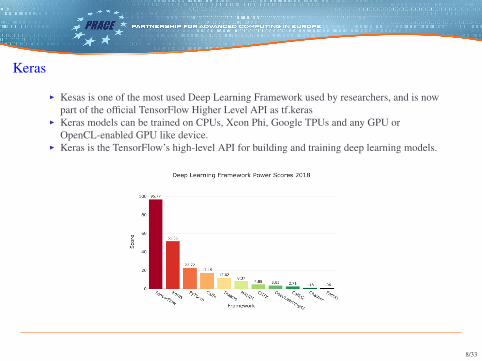
I Kesas is one of the most used Deep Learning Framework used by researchers, and is nowpart of the official TensorFlow Higher Level API as tf.keras

I Keras models can be trained on CPUs, Xeon Phi, Google TPUs and any GPU orOpenCL-enabled GPU like device.

I Keras is the TensorFlow’s high-level API for building and training deep learning models.

8/33

Building models with Keras

I The core data structure of Keras is the Model which is basically a container of one or moreLayers.

I There are two main types of models available in Keras: the Sequential model and theModel class, the latter used to create advanced models.

I The simplest type of model is the Sequential model, which is a linear stack of layers. Eachlayer is added to the model using the .add() method of the Sequential model object.

I The model needs to know what input shape it should expect. The first layer in a Sequentialmodel (and only the first) needs to receive information about its input shape, specifing theinput_shape argument. The following layers can do automatic shape inference from theshape of its predecessor layer.

9/33

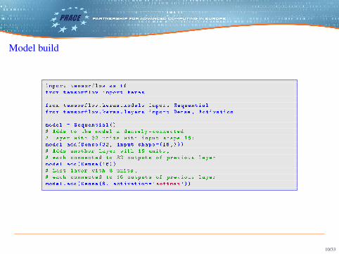
Model build

import tensorflow as tffrom tensorflow import keras

from tensorflow.keras.models import Sequentialfrom tensorflow.keras.layers import Dense , Activation

model = Sequential ()# Adds to the model a densely -connected# layer with 32 units with input shape 16:model.add(Dense (32, input_shape =(16,)))# Adds another layer with 16 units ,# each connected to 32 outputs of previous layermodel.add(Dense (16))# Last layer with 8 units ,# each connected to 16 outputs of previous layermodel.add(Dense(8, activation='softmax '))

10/33

Activation functions

I The activation argument specifies the activation function for the current layer. By default,no activation is applied.

I The softmax activation function normalize the output to a probability distribution. Iscommonly used in the last layer of a model. To select a single output in a classificationproblem the most probable one can be selected.

I The ReLU (Rectified Linear Unit), max(0,x), is commonly used as activation function forthe hidden layers.

I Many other activation functions are available or easily defined as well as layer types.

11/33

Model compile

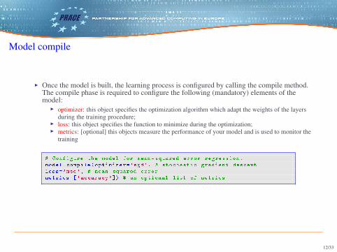
I Once the model is built, the learning process is configured by calling the compile method.The compile phase is required to configure the following (mandatory) elements of themodel:

I optimizer: this object specifies the optimization algorithm which adapt the weights of the layersduring the training procedure;

I loss: this object specifies the function to minimize during the optimization;I metrics: [optional] this objects measure the performance of your model and is used to monitor the

training

# Configure the model for mean -squared error regression.model.compile(optimizer='sgd', # stochastic gradient descentloss='mse', # mean squared errormetrics =['accuracy ']) # an optional list of metrics

12/33

Model compile

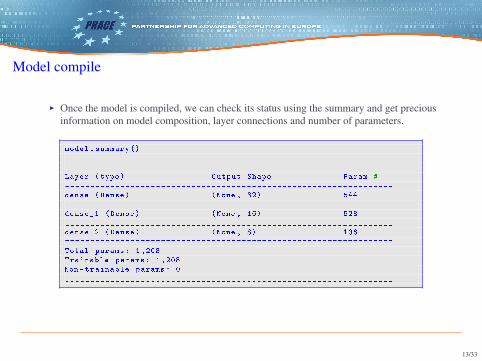
I Once the model is compiled, we can check its status using the summary and get preciousinformation on model composition, layer connections and number of parameters.

model.summary ()

_________________________________________________________________Layer (type) Output Shape Param #=================================================================dense (Dense) (None , 32) 544_________________________________________________________________dense_1 (Dense) (None , 16) 528_________________________________________________________________dense_2 (Dense) (None , 8) 136=================================================================Total params: 1,208Trainable params: 1,208Non -trainable params: 0_________________________________________________________________

13/33

Model training

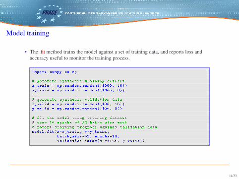
I The .fit method trains the model against a set of training data, and reports loss andaccuracy useful to monitor the training process.

import numpy as np

# generate synthetic training datasetx_train = np.random.random ((1000 , 16))y_train = np.random.random ((1000 , 8))

# generate synthetic validation datax_valid = np.random.random ((100, 16))y_valid = np.random.random ((100, 8))

# fit the model using training dataset# over 10 epochs of 32 batch size each# report training progress against validation datamodel.fit(x=x_train , y=y_train ,

batch_size =32, epochs =10,validation_data =(x_valid , y_valid))

14/33

Model evaluation and prediction

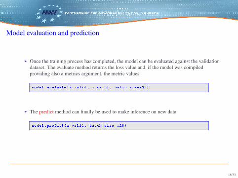
I Once the training process has completed, the model can be evaluated against the validationdataset. The evaluate method returns the loss value and, if the model was compiledproviding also a metrics argument, the metric values.

model.evaluate(x_valid , y_valid , batch_size =32)

I The predict method can finally be used to make inference on new data

model.predict(x_valid , batch_size =128)

15/33

Model saving and restore

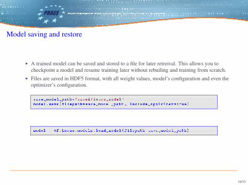
I A trained model can be saved and stored to a file for later retreival. This allows you tocheckpoint a model and resume training later without rebuiling and training from scratch.

I Files are saved in HDF5 format, with all weight values, model’s configuration and even theoptimizer’s configuration.

save_model_path='saved/intro_model 'model.save(filepath=save_model_path , include_optimizer=True)

model = tf.keras.models.load_model(filepath=save_model_path)

16/33

Try it out

17/33

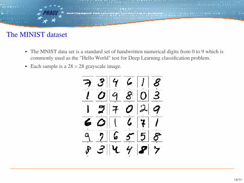
The MINIST dataset

I The MNIST data set is a standard set of handwritten numerical digits from 0 to 9 which iscommonly used as the "Hello World" test for Deep Learning classification problem.

I Each sample is a 28×28 grayscale image.

18/33

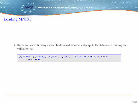
Loading MNIST

I Keras comes with many dataset built in and automatically splits the data into a training andvalidation set.

(x_train , y_train), (x_test , y_test) = tf.keras.datasets.mnist.load_data ()

19/33

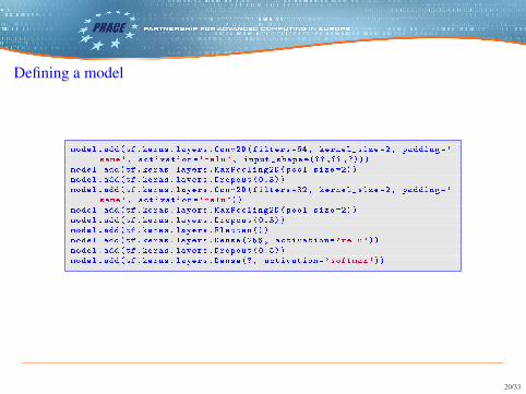
Defining a model

model.add(tf.keras.layers.Conv2D(filters =64, kernel_size =2, padding='same', activation='relu', input_shape =(?? ,?? ,?)))

model.add(tf.keras.layers.MaxPooling2D(pool_size =2))model.add(tf.keras.layers.Dropout (0.3))model.add(tf.keras.layers.Conv2D(filters =32, kernel_size =2, padding='

same', activation='relu'))model.add(tf.keras.layers.MaxPooling2D(pool_size =2))model.add(tf.keras.layers.Dropout (0.3))model.add(tf.keras.layers.Flatten ())model.add(tf.keras.layers.Dense (256, activation='relu'))model.add(tf.keras.layers.Dropout (0.5))model.add(tf.keras.layers.Dense(?, activation='softmax '))

20/33

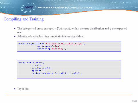
Compiling and Training

I The categorical cross entropy, −∑p(x)q(x), with p the true distribution and q the expectedone.

I Adam is adaptive learning rate optimization algorithm.

model.compile(loss='categorical_crossentropy ',optimizer='adam',metrics =['accuracy '])

model.fit(x_train ,y_train ,batch_size =64,epochs =10,validation_data =(x_valid , y_valid),)

I Try it out

21/33

Callbacks

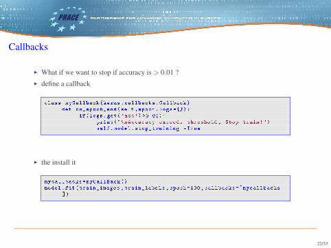
I What if we want to stop if accuracy is > 0.01 ?I define a callback

class myCallback(keras.callbacks.Callback)def on_epoch_end(self ,epoch ,logs ={}):

if(logs.get('acc') >0.01):print("\nAccuracy exceeds threshold , Stop train!")self.model.stop_training =True

I the install it

mycallbacks=myCallBack ()model.fit(train_images ,train_labels ,epoch =100, callbacks =[ mycallbacks

])

22/33

Callbacks

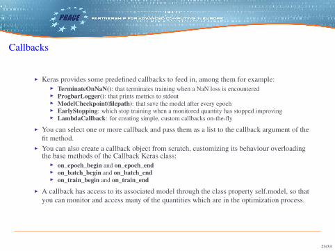
I Keras provides some predefined callbacks to feed in, among them for example:I TerminateOnNaN(): that terminates training when a NaN loss is encounteredI ProgbarLogger(): that prints metrics to stdoutI ModelCheckpoint(filepath): that save the model after every epochI EarlyStopping: which stop training when a monitored quantity has stopped improvingI LambdaCallback: for creating simple, custom callbacks on-the-fly

I You can select one or more callback and pass them as a list to the callback argument of thefit method.

I You can also create a callback object from scratch, customizing its behaviour overloadingthe base methods of the Callback Keras class:

I on_epoch_begin and on_epoch_endI on_batch_begin and on_batch_endI on_train_begin and on_train_end

I A callback has access to its associated model through the class property self.model, so thatyou can monitor and access many of the quantities which are in the optimization process.

23/33

Introduction

Keras

Distributed Deep Learning

24/33

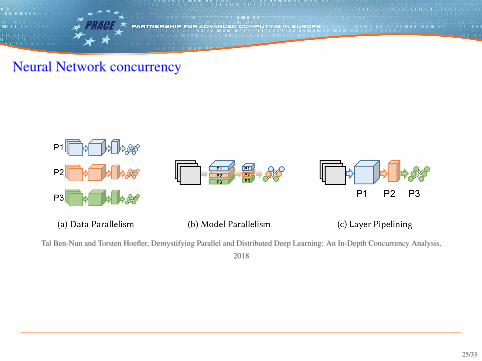
Neural Network concurrency

Tal Ben-Nun and Torsten Hoefler, Demystifying Parallel and Distributed Deep Learning: An In-Depth Concurrency Analysis,

2018

25/33

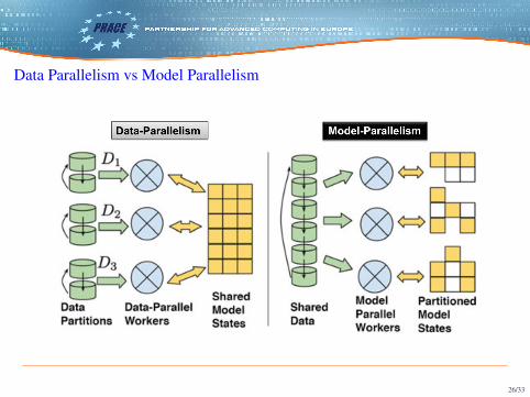
Data Parallelism vs Model Parallelism

26/33

Hardware and Libraries

I It is not only a matter of computational power:I CPU (MKL-DNN)I GPU (cuDNN)I FPGAI TPU

I Input/OutputI SSDI Parallel file system (if you run in parallel)

I Communication and interconnection too, if you are running in distributed modeI MPII gRPC + verbs (RDMA)I NCCL

27/33

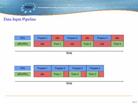
Data Input Pipeline

28/33

CPU optimizations

I Built from source with all of the instructions supported by the target CPU and theMKL-DNN option for Intel® CPU.

I Adjust thread poolsI intra_op_parallelism_threads: Nodes that can use multiple threads to parallelize their execution

will schedule the individual pieces into this pool. (OMP_NUM_THREADS)I inter_op_parallelism_threads: All ready nodes are scheduled in this pool

config = tf.ConfigProto ()config.intra_op_parallelism_threads = 44config.inter_op_parallelism_threads = 44tf.session(config=config)

I The MKL is optimized for NCHW (default NHWC) data format and use the followingvariables to tune performance: KMP_BLOCKTIME, KMP_AFFINITY ,OMP_NUM_THREADS

29/33

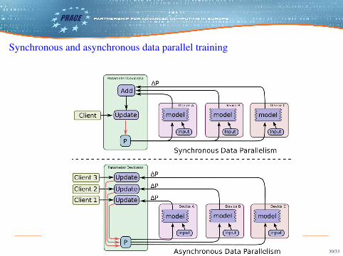
Synchronous and asynchronous data parallel training

TensorFlow: Large-Scale Machine Learning on Heterogeneous Distributed Systems, 2016

30/33

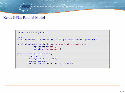
Keras GPUs Parallel Model

model = keras.Sequential ()...gpus=4parallel_model = keras.utils.multi_gpu_model(model , gpus=gpus)

parallel_model.compile(loss='categorical_crossentropy ',optimizer='adam',metrics =['accuracy '])

parallel_model.fit(x_train ,y_train ,batch_size=batch_size ,epochs=epochs ,validation_data =(x_valid , y_valid),)

31/33

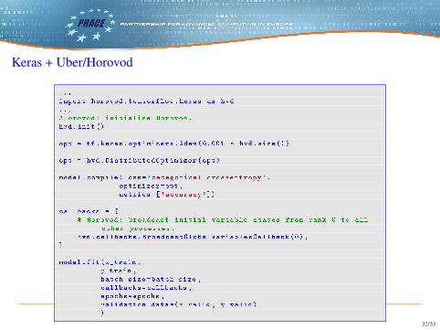
Keras + Uber/Horovod

...import horovod.tensorflow.keras as hvd...#Horovod: initialize Horovod.hvd.init()

opt = tf.keras.optimizers.Adam (0.001 * hvd.size())

opt = hvd.DistributedOptimizer(opt)

model.compile(loss='categorical_crossentropy ',optimizer=opt ,metrics =['accuracy '])

callbacks = [# Horovod: broadcast initial variable states from rank 0 to all

other processes.hvd.callbacks.BroadcastGlobalVariablesCallback (0),

]

model.fit(x_train ,y_train ,batch_size=batch_size ,callbacks=callbacks ,epochs=epochs ,validation_data =(x_valid , y_valid))

32/33

Other References

I HorovodI NCCLI MNISTI CIFAR datasetsI Deeplearning.ai youtube channel

33/33