AuTO: Scaling Deep Reinforcement Learningfor Datacenter-Scale Automatic Traic Optimization

Li Chen, Justinas Lingys, Kai Chen, Feng Liu†SING Lab, Hong Kong University of Science and Technology, †SAIC Motors

{lchenad,jlingys,kaichen}@cse.ust.hk,liufeng@saicmotor.com

ABSTRACTTrac optimizations (TO, e.g. ow scheduling, load balanc-ing) in datacenters are dicult online decision-making prob-lems. Previously, they are done with heuristics relying onoperators’ understanding of the workload and environment.Designing and implementing proper TO algorithms thus takeat least weeks. Encouraged by recent successes in applyingdeep reinforcement learning (DRL) techniques to solve com-plex online control problems, we study if DRL can be used forautomatic TO without human-intervention. However, ourexperiments show that the latency of current DRL systemscannot handle ow-level TO at the scale of current datacen-ters, because short ows (which constitute the majority oftrac) are usually gone before decisions can be made.

Leveraging the long-tail distribution of datacenter trac,we develop a two-level DRL system, AuTO, mimicking thePeripheral & Central Nervous Systems in animals, to solvethe scalability problem. Peripheral Systems (PS) reside onend-hosts, collect ow information, and make TO decisionslocally with minimal delay for short ows. PS’s decisionsare informed by a Central System (CS), where global tracinformation is aggregated and processed. CS further makesindividual TO decisions for long ows. With CS&PS, AuTOis an end-to-end automatic TO system that can collect net-work information, learn from past decisions, and perform ac-tions to achieve operator-dened goals. We implement AuTOwith popular machine learning frameworks and commodityservers, and deploy it on a 32-server testbed. Compared toexisting approaches, AuTO reduces the TO turn-around timefrom weeks to ∼100 milliseconds while achieving superior

Permission to make digital or hard copies of all or part of this work forpersonal or classroom use is granted without fee provided that copiesare not made or distributed for prot or commercial advantage and thatcopies bear this notice and the full citation on the rst page. Copyrightsfor components of this work owned by others than the author(s) mustbe honored. Abstracting with credit is permitted. To copy otherwise, orrepublish, to post on servers or to redistribute to lists, requires prior specicpermission and/or a fee. Request permissions from permissions@acm.org.SIGCOMM ’18, August 20–25, 2018, Budapest, Hungary© 2018 Copyright held by the owner/author(s). Publication rights licensedto the Association for Computing Machinery.ACM ISBN 978-1-4503-5567-4/18/08. . . $15.00https://doi.org/10.1145/3230543.3230551

performance. For example, it demonstrates up to 48.14% re-duction in average ow completion time (FCT) over existingsolutions.

CCS CONCEPTS• Networks → Network resources allocation; Tracengineering algorithms; Data center networks; • Com-puting methodologies → Reinforcement learning;

KEYWORDSDatacenter Networks, Reinforcement Learning, Trac Opti-mization

1 INTRODUCTIONDatacenter trac optimizations (TO, e.g. ow/coow sched-uling [1, 4, 8, 14, 18, 19, 29, 61], congestion control [3, 10],load balancing &routing [2]) have signicant impact on ap-plication performance. Currently, TO is dependent on hand-crafted heuristics for varying trac load, ow size distri-bution, trac concentration, etc. When parameter settingmismatches trac, TO heuristics may suer performancepenalty. For example, in PIAS [8], thresholds are calculatedbased on a long term ow size distribution, and is proneto mismatch the current/true size distribution in run-time.Under mismatch scenarios, performance degradation can beas much as 38.46% [8]. pFabric [4] shares the same problemwhen implemented with limited switch queues: for certaincases the average FCT can be reduced by over 30% even if thethresholds are carefully optimized. Furthermore, in coowscheduling, xed thresholds in Aalo [18] depend on the op-erator’s ability to choose good values upfront, since there isno run-time adaptation.

Apart from parameter-environment mismatches, the turn-around time of designing TO heuristics is long—at leastweeks. Because they require operator insight, applicationknowledge, and trac statistics collected over a long periodof time. A typical process includes: rst, deploying a mon-itoring system to collect end-host and/or switch statistics;second, after collecting enough data, operators analyze thedata, design heuristics, and test it using simulation tools andoptimization tools to nd suitable parameter settings; nally,

SIGCOMM ’18, August 20–25, 2018, Budapest, Hungary L. Chen et al.

tested heuristics are enforced1 (with application modica-tions [19, 61], OS kernel module [8, 14], switch congura-tions [10], or any combinations of the above).

Automating the TO process is thus appealing, and we de-sire an automated TO agent that can adapt to voluminous,uncertain, and volatile datacenter trac, while achievingoperator-dened goals. In this paper, we investigate rein-forcement learning (RL) techniques [55], as RL is the subeldof machine learning concerned with decision making andaction control. It studies how an agent can learn to achievegoals in a complex, uncertain environment. An RL agentobserves previous environment states and rewards, then de-cides an action in order to maximize the reward. RL hasachieved good results in many dicult environments in re-cent years with advances in deep neural networks (DNN):DeepMind’s Atari results [40] and AlphaGo [52] used deepRL (DRL) algorithms which make few assumptions abouttheir environments, and thus can be generalized in other set-tings. Inspired by these results, we are motivated to enableDRL for automatic datacenter TO.We started by verifying DRL’s eectiveness in TO. We

implemented a ow-level centralized TO system with a basicDRL algorithm, policy gradient [55]. However, in our exper-iments (§2.2), even this simple algorithm running on cur-rent machine learning software frameworks2 and advancedhardware (GPU) cannot handle trac optimization tasks atthe scale of production datacenters (>105 servers). The cruxis the computation time (∼100ms): short ows (which con-stitute the majority of the ows) are gone before the DRLdecisions come back, rendering most decisions useless.

Therefore, in this paper we try to answer the key question:How to enable DRL-based automatic TO at datacenter-scale?To make DRL scalable, we rst need to understand the long-tail distribution of datacenter trac [3, 11, 33]: most of theows are short ows3, but most of the bytes are from longows. Thus, TO decisions for short ows must be generatedquickly; whereas decisions for long ows aremore inuentialas they take longer time to nish.

We presentAuTO, an end-to-endDRL system for datacenter-scale TO that works with commodity hardware. AuTO is atwo-level DRL system, mimicking the Peripheral & CentralNervous Systems in animals. Peripheral Systems (PS) run onall end-hosts, collect ow information, and make instant TOdecisions locally for short ows. PS’s decisions are informedby the Central System (CS), where global trac information

1After the heuristic is designed, its parameters can usually be computed ina short time for average scenarios: minutes [8, 14, 19] or hours [61]. AuTOseeks to automate the entire TO design process, rather than just parameterselection.2e.g. TensorFlow [57], PyTorch [48], Ray [42]3The threshold between short and long ows is dynamically determined inAuTO based on current trac distribution (§4).

are aggregated and processed. CS further makes individualTO decisions for long ows which can tolerate longer pro-cessing delays.

The key to AuTO’s scalability is to detach time-consumingDRL processing from quick action-taking for short ows.To achieve this, we adopt Multi-Level Feedback Queueing(MLFQ) [8] for PS to schedule ows guided by a set of thresh-olds. Every new ow starts at the rst queue with highestpriority, and is gradually demoted to lower queues after itssent bytes pass certain thresholds. Using MLFQ, AuTO’s PSmakes per-ow decisions instantly upon local information(bytes-sent and thresholds)4, while the thresholds are stilloptimized by a DRL algorithm in the CS over a relativelylonger period of time. In this way, global TO decisions aredelivered to PS in the form of MLFQ thresholds (which ismore delay-tolerant), enabling AuTO to make globally in-formed TO decisions for the majority of ows with onlylocal information. Furthermore, MLFQ naturally separatesshort and long ows: short ows complete in the rst fewqueues, and long ows descend down to the last queue. Forlong ows, CS centrally processes them individually using adierent DRL algorithm to determine routing, rate limiting,and priority.We have implemented an AuTO prototype using Python.

AuTO is thus compatible with popular learning frameworks,such as Keras/TensorFlow. This allows both networkingand machine learning community to easily develop and testnew algorithms, because software components in AuTO arereusable in other RL projects in datacenter.We further build a testbed with 32 servers connected by

2 switches to evaluate AuTO. Our experiments show that,for trac with stable load and ow size distribution, AuTO’sperformance improvement is up to 48.14% compared to stan-dard heuristics (shortest-job-rst and least-attained-service-rst) after 8 hours of training. AuTO is also shown to learnsteadily and adapt across temporally and spatially heteroge-neous trac: after only 8 hours of training, AuTO achieves8.71% (9.18%) reduction in average (tail) FCT compared toheuristics.In the following, we rst overview DRL and reveal why

current DRL systems fail to work at large scale in §2. Wedescribe system design in §3, as well as the DRL formulationsand solutions in §4. We implement AuTO in §5, and evaluateit with extensive experiments in §6 using a realistic testbed.Finally, we review related works in §7, and conclude in §8.

2 BACKGROUND AND MOTIVATIONIn this section, we rst overview the RL background. Then,we describe and apply a basic RL algorithm, policy gradient,

4For short ows, AuTO relies on ECMP[30] (which is also not centrallycontrolled) for routing/load-balancing and makes no rate-limiting decisions.

AuTO: Scaling Deep Reinforcement Learningfor Datacenter-Scale Automatic Traic Optimization SIGCOMM ’18, August 20–25, 2018, Budapest, Hungary

Figure 1: A general reinforcement learning setting us-ing neural network as policy representation.to enable ow scheduling in TO. Finally, we show the prob-lem of an RL system running PG using testbed experiments,motivating AuTO.

2.1 Deep Reinforcement Learning (DRL)As shown in Figure 1, environment is the surroundings ofthe agent with which the agent can interact through ob-servations, actions, and feedback (rewards) on actions [55].Specically, in each time step t , the agent observes state st ,and chooses action at . The state of the environment thentransits to st+1, and the agent receives reward rt . The statetransitions and rewards are stochastic and Markovian [36].The objective of learning is to maximize the expected cumu-lative discounted reward E[∑∞t=0γ trt ] where γt∈(0,1] is thediscounting factor.The RL agent takes actions based on a policy, which is

a probability distribution of taking action a in the state s:π (s,a). For most practical problems, it is infeasible to learnall possible combinations of state-action pairs, thus functionapproximation [31] technique is commonly used to learn thepolicy. A function approximator πθ (s,a) is parameterized byθ , whose size is much smaller (thus mathematically tractable)than the number of all possible state-action pairs. Functionapproximator can have many forms, and recently, deep neu-ral networks (DNNs) have been shown to solve practical,large-scale dynamic control problems similar to ow sched-uling. Therefore, we also use DNN as the representation offunction approximator in AuTO.With function approximation, the agent learns by updat-

ing the function parameters θ with the state st , action at ,and the corresponding reward rt in each time period/step t .We focus on one class of updating algorithms that learn byperforming gradient-descent on the policy parameters. Thelearning involves updating the parameters (link weights)of a DNN so that the aforementioned objective could bemaximized.

θ ← θ + α∑t

∇θ loд πθ (st ,at )vt (1)

Training of the agent’s DNN adopts a variant of the well-known REINFORCE algorithm [56]. This variant uses a mod-ied version of Equation (1), which alleviates the drawbacksof the algorithm: convergence speed and variance. To mit-igate the drawbacks, Monte Carlo Method [28] is used tocompute an empirical reward, vt , and a baseline value (thecumulative average of experienced rewards per server) isused for reducing the variance [51]. The resultant updaterule (Equation (2)) is applied to the policy DNN, due to itsvariance management and guaranteed convergence to atleast a local minimum [56]:

θ ← θ + α∑t

∇θ loд πθ (st ,at ) (vt − baseline ) (2)

2.2 Example: DRL for Flow SchedulingAs an example, we formulate the problem of ow schedulingin datacenters as a DRL problem, and describe a solutionusing the PG algorithm based on Equation (2).Flow scheduling problem We consider a datacenter net-work connecting multiple servers. For simplicity, we adoptthe big-switch assumption by previous works in ow sched-uling [4, 14], where the network is non-blocking with full-bisection bandwidth and proper load-balancing. Followingthis assumption, the ow scheduling problem is simpliedto the problem of deciding the sending order of ows. Weconsider an implementation that enables preemptive sched-uling of ows using strict priority queueing. We create Kpriority queues for ows in each server [23], and enforcestrict priority queuing among them. K priority queues arealso congured in the switches, similar to [8]. The priority ofeach ow can be changed dynamically to enable pre-emption.The packet of each ow is tagged with its current prioritynumber, and will be placed in the same queue throughoutthe entire datacenter fabric.DRL formulationAction Space: The action provided by the agent is a mappingfrom active ows to priorities: for each active ow f , at timestep t , its priority is pt ( f )∈[1,K].State space: The big-switch assumption allows for a muchsimplied state space. As routing and load balancing are outof our concern, the state space only includes the ow states.In our model, states are represented as the set of all activeows, F ta , and the set of all nished ows, F td , in the entirenetwork at current time step t . Each ow is identied byits 5-tuple [8, 38]: source/destination IP, source/destinationport numbers, and transport protocol. Active ows have an

SIGCOMM ’18, August 20–25, 2018, Budapest, Hungary L. Chen et al.

additional attribute, which is its priority; while nished owshave two additional attributes: FCT and ow size5.Rewards: Rewards are feedback to the agent on how good itsactions are. The reward can be obtained after the completionof a ow, thus is computed only on the set of nished owsF td for time step t . The average throughput of each nishedow f is Tputf =

SizefFCTf

. We model the reward as the ratiobetween the average throughputs of two consecutive timesteps.

rt=

∑f t ∈F td

Tput tf∑f t−1∈F t−1d

Tput t−1f

(3)

It signals if the previous actions have resulted in a higherper-ow throughput experienced by the agent, or it has de-graded the overall performance. The objective is to maximizethe average throughput of the network as a whole.DRL algorithm We use the update rule specied by Equa-tion (2). The DNN residing on the agent computes probabilityvectors for each new state and updates its parameters by eval-uating the action that resulted in the current state. The eval-uation step compares the previous average throughput withthe corresponding value of the current step. Based on thecomparison, an appropriate reward (either negative or posi-tive) is produced which is added to the baseline value. Thus,we can ensure that the function approximator improves withtime and can converge to a local minimum by updating DNNweights in the direction of the gradient. The update whichfollows (2) ensures that poor ow scheduling decisions arediscouraged for similar states in the future, and the goodones become more probable for similar states in the future.When the system converges, the policy achieves a sucientow scheduling mechanism for a cluster of servers.

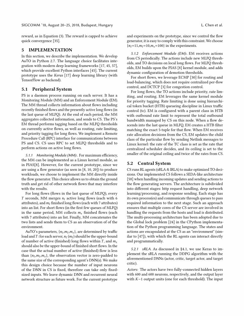
2.3 Problem IdentiedUsing the DRL problem of ow scheduling as an example,we implement PG using popular machine learning frame-works: Keras/TensorFlow, PyTorch, and Ray. We simplify theDRL agent to have only 1 hidden layer. We use two servers:DRL agent resides in one, and the other sends mock tracinformation (states) to the agent using an RPC interface. Weset the sending rate of the mock server to 1000 ows persecond (fps). We measure the processing latency of dierentimplementations at the mock server: the time between nishsending the ow information and receiving the action. Theservers are Huawei Tecal RH1288 V2 servers running 64-bitDebian 8.7, with 4-core Intel E5-1410 2.8GHz CPU, NVIDIAK40 GPU, and Broadcom 1Gbps NICs.

5Flow size and FCT can be measured when the ow ends using either OSutility[44] or application layer mechanisms[49, 61].

Figure 2: Current DRL systems are insucient.As shown in Figure2, even for small ow arrival rate of

1000fps and only 1 hidden layer, the processing delays ofall implementations are more than 60ms, during which timeany ow within 7.5MB would have nished on a 1Gbps link.For reference, using the well-known trac traces of a websearch application and a data mining application collected inMicrosoft datacenters[3, 8, 26], a 7.5MB ow is larger than99.99% and 95.13% of all ows, respectively. This means,most of the DRL actions are useless, as the correspondingows are already gone when the actions arrive.Summary Current DRL systems’ performance is not enoughto make online decisions for datacenter-scale trac. Theysuer from long processing delays even for simple algorithmsand low trac load.

3 AUTO DESIGN3.1 OverviewThe key problem of current DRL systems is the long latencybetween collection of ow information and generation ofactions. In modern datacenters with ≥10Gbps link speed,to achieve ow-level TO operations, the round-trip latencyof actions should be at least sub-millisecond. Without in-troducing specialized hardware, this is unachievable (§2.2).Using commodity hardware, the processing latency of DRLalgorithm is a hard limit. Given this constraint, how to scaleDRL for datacenter TO?

Recent studies [3, 11, 33] have shown that most datacenterows are short ows, yet most trac bytes are from longows. Informed by such long-tail distribution, our insightis to delegate most short ow operations to the end-host,and formulate DRL algorithms to generate long-term (sub-second) TO decisions for long ows.

We design AuTO as a two-level system, mimicking the Pe-ripheral and Central Nervous Systems in animals. As shownin Figure 3, Peripheral Systems (PS) run on all end-hosts,collect ow information, and make TO decisions locally withminimal delay for short ows. Central System (CS) makes in-dividual TO decisions for long ows that can tolerate longerprocessing delays. Furthermore, PS’s decisions are informedby the CS where global trac information are aggregatedand processed.

AuTO: Scaling Deep Reinforcement Learningfor Datacenter-Scale Automatic Traic Optimization SIGCOMM ’18, August 20–25, 2018, Budapest, Hungary

Figure 3: AuTO overview.

Figure 4: Multi-Level Feedback Queuing.3.2 Peripheral SystemThe key to AuTO’s scalability is to enable PS to make glob-ally informed TO decisions on short ows with only localinformation. PS has two modules: an enforce module and amonitoring module.Enforcementmodule To achieve the above goal, we adoptMulti-Level FeedbackQueueing (MLFQ, introduced in PIAS [8])to schedule owswithout centralized per-ow control. Specif-ically, PS performs packet tagging in the DSCP eld of IPpackets at each end-host as shown in Figure 4. There are Kpriorities, Pi ,1≤i≤K , and (K−1) demotion thresholds, α j ,1≤j≤K−1. We congure all the switches to perform strict pri-ority queueing based on the DSCP eld. At the end host,when a new ow is initialized, its packets are tagged withP1, giving them the highest priority in the network. As morebytes are sent, the packets of this ow will be tagged withdecreasing priorities Pj (2≤j≤K), thus they are scheduledwith decreasing priorities in the network. The threshold todemote priority from Pj−1 to Pj is α j−1.With MLFQ, PS has the following properties:• It can make instant per-ow decisions based only on localinformation: bytes-sent and thresholds.

Figure 5: AuTO: A 4-queue example.• It can adapt to global trac variations. To be scalable, CSmust not directly control small ows. Instead, CS opti-mizes and sets MLFQ thresholds with global informationover a longer period of time. Thus, thresholds in PS can beupdated to adapt to trac variations. In contrast, PIAS [8]requires weeks of trac traces to update the thresholds.• It naturally separates short and long ows. As shown inFigure 5, short ows nished in the rst few queues, andlong ows drop to the last queue. Thus, CS can centrallyprocess long ows individually to make decisions on rout-ing, rate limit, and priority.

Monitoring module For CS to generate thresholds, themonitoring module collects ow sizes and completion timesof all nished ows, so that CS can update ow size distri-bution. The monitoring module also reports on-going longows that have descended into the lowest priority on itsend-host, so that CS can make individual decisions.

3.3 Central SystemThe CS is composed of twoDRL agents (RLA): short ow RLA(sRLA) is for optimizing thresholds for MLFQ, and long owRLA (lRLA) is for determining rates, routes, and prioritiesfor long ows. sRLA attempts to solve a FCT minimizationproblem, and we develop a Deep Deterministic Policy Gra-dient algorithm for this purpose. For lRLA, we use a PGalgorithm (§2.2) to generate actions for the long ows. Inthe next section, we describe the two DRL problems andsolutions.

4 DRL FORMULATIONS AND SOLUTIONSIn this section, we describe the two DRL algorithms in CS.

4.1 Optimizing MLFQ thresholdsWe consider a datacenter network connectingmultiple servers.Scheduling of ows is imposed by using K strict priorityqueues at hosts and network switches (Figure 4) by setting

SIGCOMM ’18, August 20–25, 2018, Budapest, Hungary L. Chen et al.

the DCSP eld in each of the IP headers. The longer theow is, the lower priority is assigned to the ow as it is de-moted through host priority queues in order to approximateShortest-Job-First (SJF). The packet’s priority is preservedthroughout the entire datacenter fabric till it reaches thedestination.One of the challenges of MLFQ is the calculation of the

optimal demotion thresholds for the K priority queues atthe host. Prior works [8, 9, 14] provide mathematical anal-ysis and models for optimizing the demotion thresholds:{α1,α2,...,αK−1}. Bai et al. [9] also suggest weekly/monthlyre-computation of the thresholds with collected ow-leveltraces. AuTO takes a step further and proposes a DRL ap-proach to optimizing the values of theα ’s. Unlike prior worksthat used machine learning in datacenter problems [5, 36, 60],AuTO is unique due to its target - optimization of real val-ues in continuous action space. We formulate the thresholdoptimization problem as an DRL problem and try to explorethe capabilities of DNN for modeling the complex datacenternetwork for computing the MLFQ thresholds.

As shown in §2.2, PG is a basic DRL algorithm. The agentfollows a policy πθ (a |s ) parameterized by a vector θ andimproves it with experience. However, REINFORCE andother regular PG algorithms only consider stochastic policies,πθ (a |s )=P[a |s;θ], that select action a in state s according tothe probability distribution over the action set A parame-terized by θ . PG cannot be used for value optimization prob-lem, as a value optimization problem computes real values.Therefore, we apply a variant ofDeterministic Policy Gradient(DPG) [53] for approximating optimal values {a0,a1,...,an }for the given state s such that ai=µθ (s ) f or i=0,...,n. Figure6 summarizes the major dierences between stochastic anddeterministic policies. DPG is an actor-critic [12] algorithmfor deterministic policies, which maintains a parameterizedactor function µθ for representing current policy and a criticneural network Q (s,a) that is updated using the Bellmanequation (as in Q-learning [41]). We describe the algorithmwith Equation (4,5,6) as follows: The actor samples the en-vironment and has its parameters θ updated according toEquation (4). The result of Equation (4) follows from the factthat the objective of the policy is to maximize the expectedcumulative discounted reward Equation(5) and its gradientcan be expressed in the following form Equation(5). For moredetails, please refer to [53].

θk+1 ← θk + αEs∼ρ µk

[∇θ µθ (s )∇aQ

µk (s,a)����a=µθ (s )

]

whereρµk is the state distribution at time k .(4)

J (µθ )=

∫S

ρµ (s )r (s,µθ (s ))ds

=Es∼ρ µ [r (s,µθ (s ))](5)

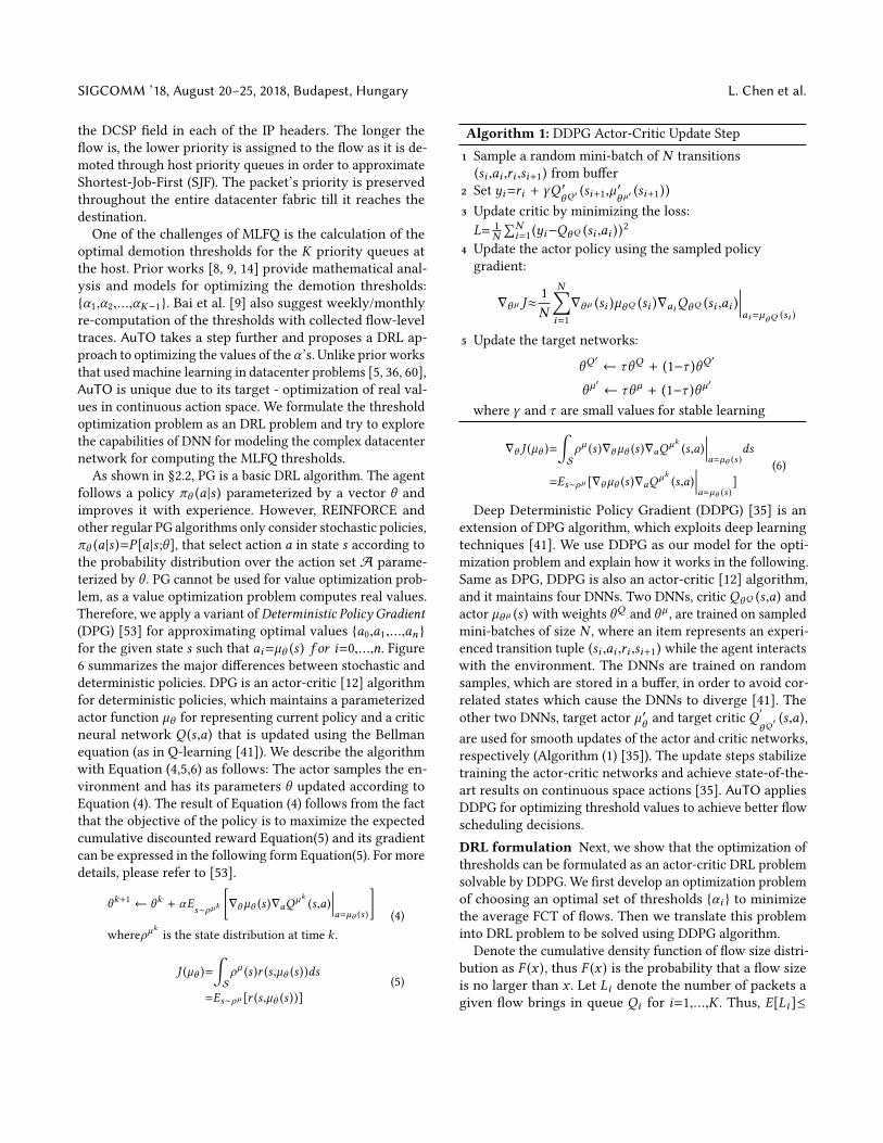
Algorithm 1: DDPG Actor-Critic Update Step1 Sample a random mini-batch of N transitions(si ,ai ,ri ,si+1) from buer

2 Set yi=ri + γQ ′θQ′ (si+1,µ′

θ µ′(si+1))

3 Update critic by minimizing the loss:L= 1

N∑N

i=1 (yi−QθQ (si ,ai ))2

4 Update the actor policy using the sampled policygradient:

∇θ µ J≈1N

N∑i=1∇θ µ (si )µθQ (si )∇aiQθQ (si ,ai )

����ai=µθQ (si )

5 Update the target networks:

θQ′

← τθQ + (1−τ )θQ ′

θ µ′

← τθ µ + (1−τ )θ µ′

where γ and τ are small values for stable learning

∇θ J (µθ )=

∫S

ρµ (s )∇θ µθ (s )∇aQµk (s,a)

����a=µθ (s )ds

=Es∼ρ µ [∇θ µθ (s )∇aQ µk (s,a)����a=µθ (s )

](6)

Deep Deterministic Policy Gradient (DDPG) [35] is anextension of DPG algorithm, which exploits deep learningtechniques [41]. We use DDPG as our model for the opti-mization problem and explain how it works in the following.Same as DPG, DDPG is also an actor-critic [12] algorithm,and it maintains four DNNs. Two DNNs, critic QθQ (s,a) andactor µθ µ (s ) with weights θQ and θ µ , are trained on sampledmini-batches of size N , where an item represents an experi-enced transition tuple (si ,ai ,ri ,si+1) while the agent interactswith the environment. The DNNs are trained on randomsamples, which are stored in a buer, in order to avoid cor-related states which cause the DNNs to diverge [41]. Theother two DNNs, target actor µ ′θ and target critic Q ′

θQ′ (s,a),

are used for smooth updates of the actor and critic networks,respectively (Algorithm (1) [35]). The update steps stabilizetraining the actor-critic networks and achieve state-of-the-art results on continuous space actions [35]. AuTO appliesDDPG for optimizing threshold values to achieve better owscheduling decisions.DRL formulation Next, we show that the optimization ofthresholds can be formulated as an actor-critic DRL problemsolvable by DDPG. We rst develop an optimization problemof choosing an optimal set of thresholds {αi } to minimizethe average FCT of ows. Then we translate this probleminto DRL problem to be solved using DDPG algorithm.

Denote the cumulative density function of ow size distri-bution as F (x ), thus F (x ) is the probability that a ow sizeis no larger than x . Let Li denote the number of packets agiven ow brings in queue Qi for i=1,...,K . Thus, E[Li ]≤

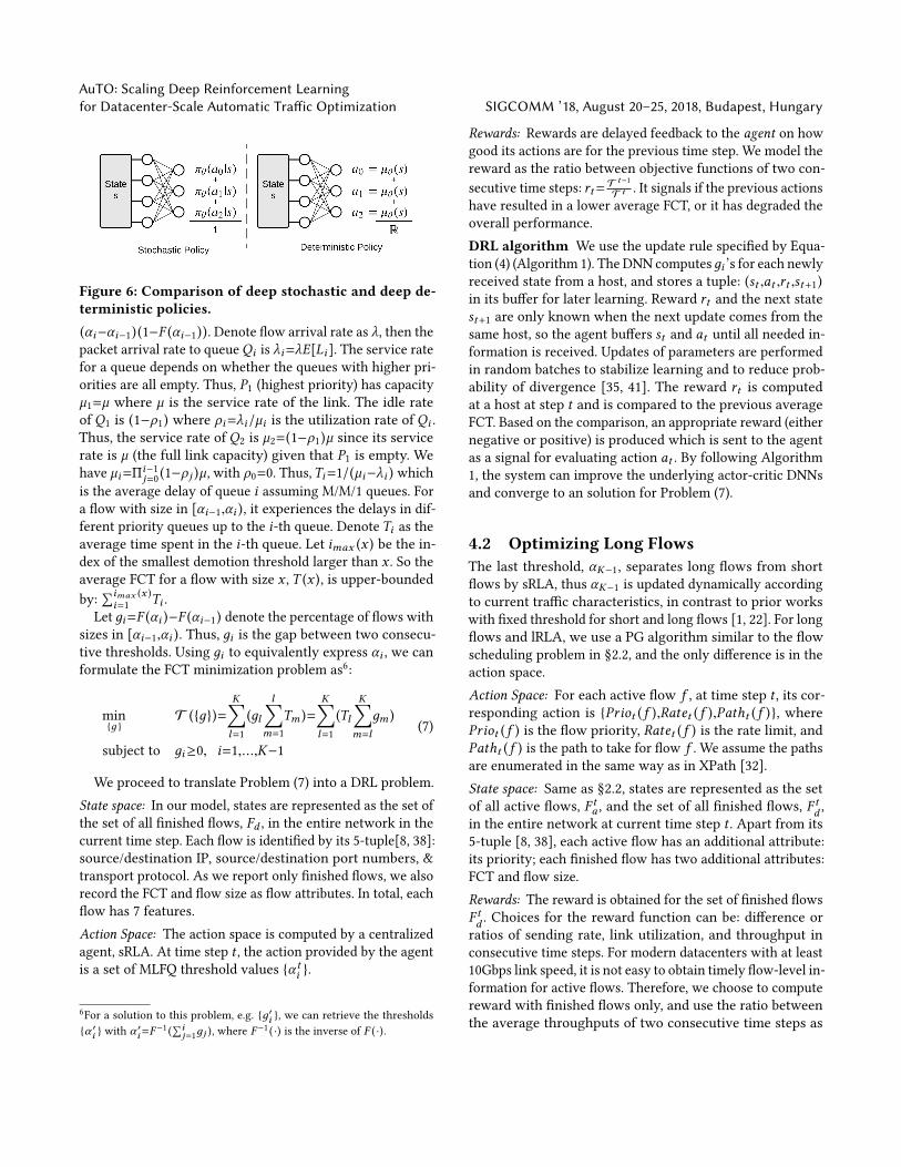
AuTO: Scaling Deep Reinforcement Learningfor Datacenter-Scale Automatic Traic Optimization SIGCOMM ’18, August 20–25, 2018, Budapest, Hungary

Figure 6: Comparison of deep stochastic and deep de-terministic policies.(αi−αi−1) (1−F (αi−1)). Denote ow arrival rate as λ, then thepacket arrival rate to queueQi is λi=λE[Li ]. The service ratefor a queue depends on whether the queues with higher pri-orities are all empty. Thus, P1 (highest priority) has capacityµ1=µ where µ is the service rate of the link. The idle rateof Q1 is (1−ρ1) where ρi=λi/µi is the utilization rate of Qi .Thus, the service rate of Q2 is µ2=(1−ρ1)µ since its servicerate is µ (the full link capacity) given that P1 is empty. Wehave µi=Πi−1

j=0 (1−ρ j )µ, with ρ0=0. Thus,Ti=1/(µi−λi ) whichis the average delay of queue i assuming M/M/1 queues. Fora ow with size in [αi−1,αi ), it experiences the delays in dif-ferent priority queues up to the i-th queue. Denote Ti as theaverage time spent in the i-th queue. Let imax (x ) be the in-dex of the smallest demotion threshold larger than x . So theaverage FCT for a ow with size x , T (x ), is upper-boundedby: ∑imax (x )

i=1 Ti .Let дi=F (αi )−F (αi−1) denote the percentage of ows with

sizes in [αi−1,αi ). Thus, дi is the gap between two consecu-tive thresholds. Using дi to equivalently express αi , we canformulate the FCT minimization problem as6:

min{д }

T ({д})=K∑l=1

(дl

l∑m=1

Tm )=K∑l=1

(Tl

K∑m=l

дm )

subject to дi≥0, i=1,...,K−1(7)

We proceed to translate Problem (7) into a DRL problem.State space: In our model, states are represented as the set ofthe set of all nished ows, Fd , in the entire network in thecurrent time step. Each ow is identied by its 5-tuple[8, 38]:source/destination IP, source/destination port numbers, &transport protocol. As we report only nished ows, we alsorecord the FCT and ow size as ow attributes. In total, eachow has 7 features.Action Space: The action space is computed by a centralizedagent, sRLA. At time step t , the action provided by the agentis a set of MLFQ threshold values {α ti }.

6For a solution to this problem, e.g. {д′i }, we can retrieve the thresholds{α ′i } with α

′i=F

−1 (∑ij=1дj ), where F

−1 ( ·) is the inverse of F ( ·).

Rewards: Rewards are delayed feedback to the agent on howgood its actions are for the previous time step. We model thereward as the ratio between objective functions of two con-secutive time steps: rt= T

t−1

T t . It signals if the previous actionshave resulted in a lower average FCT, or it has degraded theoverall performance.DRL algorithm We use the update rule specied by Equa-tion (4) (Algorithm 1). The DNN computesдi ’s for each newlyreceived state from a host, and stores a tuple: (st ,at ,rt ,st+1)in its buer for later learning. Reward rt and the next statest+1 are only known when the next update comes from thesame host, so the agent buers st and at until all needed in-formation is received. Updates of parameters are performedin random batches to stabilize learning and to reduce prob-ability of divergence [35, 41]. The reward rt is computedat a host at step t and is compared to the previous averageFCT. Based on the comparison, an appropriate reward (eithernegative or positive) is produced which is sent to the agentas a signal for evaluating action at . By following Algorithm1, the system can improve the underlying actor-critic DNNsand converge to an solution for Problem (7).

4.2 Optimizing Long FlowsThe last threshold, αK−1, separates long ows from shortows by sRLA, thus αK−1 is updated dynamically accordingto current trac characteristics, in contrast to prior workswith xed threshold for short and long ows [1, 22]. For longows and lRLA, we use a PG algorithm similar to the owscheduling problem in §2.2, and the only dierence is in theaction space.Action Space: For each active ow f , at time step t , its cor-responding action is {Priot ( f ),Ratet ( f ),Patht ( f )}, wherePriot ( f ) is the ow priority, Ratet ( f ) is the rate limit, andPatht ( f ) is the path to take for ow f . We assume the pathsare enumerated in the same way as in XPath [32].State space: Same as §2.2, states are represented as the setof all active ows, F ta , and the set of all nished ows, F td ,in the entire network at current time step t . Apart from its5-tuple [8, 38], each active ow has an additional attribute:its priority; each nished ow has two additional attributes:FCT and ow size.Rewards: The reward is obtained for the set of nished owsF td . Choices for the reward function can be: dierence orratios of sending rate, link utilization, and throughput inconsecutive time steps. For modern datacenters with at least10Gbps link speed, it is not easy to obtain timely ow-level in-formation for active ows. Therefore, we choose to computereward with nished ows only, and use the ratio betweenthe average throughputs of two consecutive time steps as

SIGCOMM ’18, August 20–25, 2018, Budapest, Hungary L. Chen et al.

reward, as in Equation (3). The reward is capped to achievequick convergence [35].

5 IMPLEMENTATIONIn this section, we describe the implementation. We developAuTO in Python 2.7. The language choice facilitates inte-gration with modern deep learning frameworks [17, 45, 57],which provide excellent Python interfaces [45]. The currentprototype uses the Keras [17] deep learning library (withTensorFlow as backend).

5.1 Peripheral SystemPS is a daemon process running on each server. It has aMonitoring Module (MM) and an Enforcement Module (EM).The MM thread collects information about ows includingrecently nished ows and the presently active long ows (inthe last queue of MLFQ). At the end of each period, the MMaggregates collected information, and sends to CS. The PS’sEM thread performs tagging based on the MLFQ thresholdson currently active ows, as well as routing, rate limiting,and priority tagging for long ows. We implement a RemoteProcedure Call (RPC) interface for communications betweenPS and CS. CS uses RPC to set MLFQ thresholds and toperform actions on active long ows.

5.1.1 Monitoring Module (MM):. For maximum eciency,the MM can be implemented as a Linux kernel module, asin PIAS[8]. However, for the current prototype, since weare using a ow generator (as seen in [8, 10, 20]) to produceworkloads, we choose to implement the MM directly insidethe ow generator. This choice allows us to obtain the groundtruth and get rid of other network ows that may interferewith the results.

For long ows (ows in the last queue of MLFQ), everyT seconds, MM merges nl active long ows (each with 6attributes), andml nished long ows (each with 7 attributes)into an list. For short ows (in the rst few queues of MLFQ)in the same period, MM collects ms nished ows (eachwith 7 attributes) into an list. Finally, MM concatenates thetwo lists and sends them to CS as an observation of of theenvironment.

AuTO’s parameters, {nl ,ml ,ms }, are determined by tracload andT : for each server,nl (ml ) should be the upper-boundof number of active (nished) long ows within T , andmsshould also be the upper-bound of nished short ows. In thecase that the actual number of active (nished) ow is lessthan {nl ,ml ,ms }, the observation vector is zero-padded tothe same size of the corresponding agent’s DNN(s). We makethis design choice because the number of input neuronsof the DNN in CS is xed, therefore can take only xed-sized inputs. We leave dynamic DNN and recurrent neuralnetwork structure as future work. For the current prototype

and experiments on the prototype, since we control the owgenerator, it is easy to complywith this constraint.We choose{nl=11,ml=10,ms=100} in the experiments.

5.1.2 Enforcement Module (EM):. EM receives actionsfrom CS periodically. The actions include new MLFQ thresh-olds, and TO decisions on local long ows. For MLFQ thresh-olds, EM builds upon the PIAS [8] kernel module, and addsdynamic conguration of demotion thresholds.For short ows, we leverage ECMP [30] for routing and

load-balancing, which does not require centralized per-owcontrol, and DCTCP [3] for congestion control.For long ows, the TO actions include priority, rate lim-

iting, and routing. EM leverages the same kernel modulefor priority tagging. Rate limiting is done using hierarchi-cal token bucket (HTB) queueing discipline in Linux traccontrol (tc). EM is congured with a parent class in HTBwith outbound rate limit to represent the total outboundbandwidth managed by CS on this node. When a ow de-scends into the last queue in MLFQ, EM creates a HTB ltermatching the exact 5-tuple for that ow. When EM receivesrate allocation decisions from the CS, EM updates the childclass of the particular ow by sending Netlink messages toLinux kernel: the rate of the TC class is set as the rate thatcentralized scheduler decides, and its ceiling is set to thesmaller of the original ceiling and twice of the rates from CS.

5.2 Central SystemCS runs RL agents (sRLA& lRLA) to make optimized TO deci-sions. Our implemented CS follows a SEDA-like architecture[58] when handling incoming updates and sending actions tothe ow generating servers. The architecture is subdividedinto dierent stages: http request handling, deep networklearning/processing, and response sending. Each stage hasits own process(es) and communicate through queues to passrequired information to the next stage. Such an approachensures that multiple cores of the CS server are involved inhandling the requests from the hosts and load is distributed.The multi-processing architecture has been adopted due tothe Global lock problem [24] in the CPython implementa-tion of the Python programming language. The states andactions are encapsulated at the CS as an "environment" (sim-ilar to [47]), with which the RL agents can interact directlyand programmatically.

5.2.1 sRLA. As discussed in §4.1, we use Keras to im-plement the sRLA running the DDPG algorithm with theaforementioned DNNs (actor, critic, target actor, and targetcritic).Actors: The actors have two fully-connected hidden layerswith 600 and 600 neurons, respectively, and the output layerwith K−1 output units (one for each threshold). The input

AuTO: Scaling Deep Reinforcement Learningfor Datacenter-Scale Automatic Traic Optimization SIGCOMM ’18, August 20–25, 2018, Budapest, Hungary

layer takes states (700 features per-server (ms=100)) andoutputs MLFQ thresholds for a host server for time step t .Critics: The critics are implemented with three hidden layers,thus the networks are a bit more complicated as comparedto the actor network. Since the critic is supposed to ’criticize’the actor for bad decisions and ’compliment’ for good ones,the critic neural network also takes as its input the outputs ofthe actor. However, as [53] suggests, the actor outputs are notdirect inputs, but are only fed into the critic’s network at ahidden layer. Therefore, the critic has two hidden layers sameas the actor and one extra hidden layer which concatenatesthe actor’s outputs with the outputs of its own second hiddenlayer, resulting in one additional hidden layer. This hiddenlayer eventually is fed into the output layer consisting of oneoutput unit - approximated value for the observed/receivedstate.The neural networks are trained on a batch of observa-

tions periodically by sampling from a buer of experience:{st ,at ,rt ,st+1} . The training process is described in Algorithm(1).

5.2.2 lRLA. For lRLA, we also use Keras to implementthe PG algorithm with a fully connected NN with 10 hiddenlayer of 300 neurons. The RL agent takes a state (136 featuresper-server (nl=11,ml=10)) and outputs probabilities for theactions for all the active ows.Summary The hyper-parameters (structure, number oflayer, height, and width of DNN) are chosen based on a fewempirical training sessions. Our observation is that morecomplicated DNNs with more hidden layers and more pa-rameters took longer to train and did not perform muchbetter than the chosen topologies. Overall, we nd that suchRLA congurations leads to good system performance andis rather reasonable considering the importance of computa-tion delay, as we reveal next in the evaluations.

6 EVALUATIONIn this section, we evaluate the performance of AuTO usingreal testbed experiments. We seek to understand: 1) Withstable trac (ow size distribution and trac load are xed),how does AuTO compare to standard heuristics? 2) For vary-ing trac characteristics, can AuTO adapt? 3) how fast canAuTO respond to trac dynamics? 4) what are the perfor-mance overheads and overall scalability?Summary of results (grouped by scenarios):

• Homogeneous: For trac with xed ow size distribu-tion and load, AuTO-generated thresholds converge, anddemonstrate similar or better performance compared tostandard heuristics, with up to 48.14% average FCT reduc-tion.

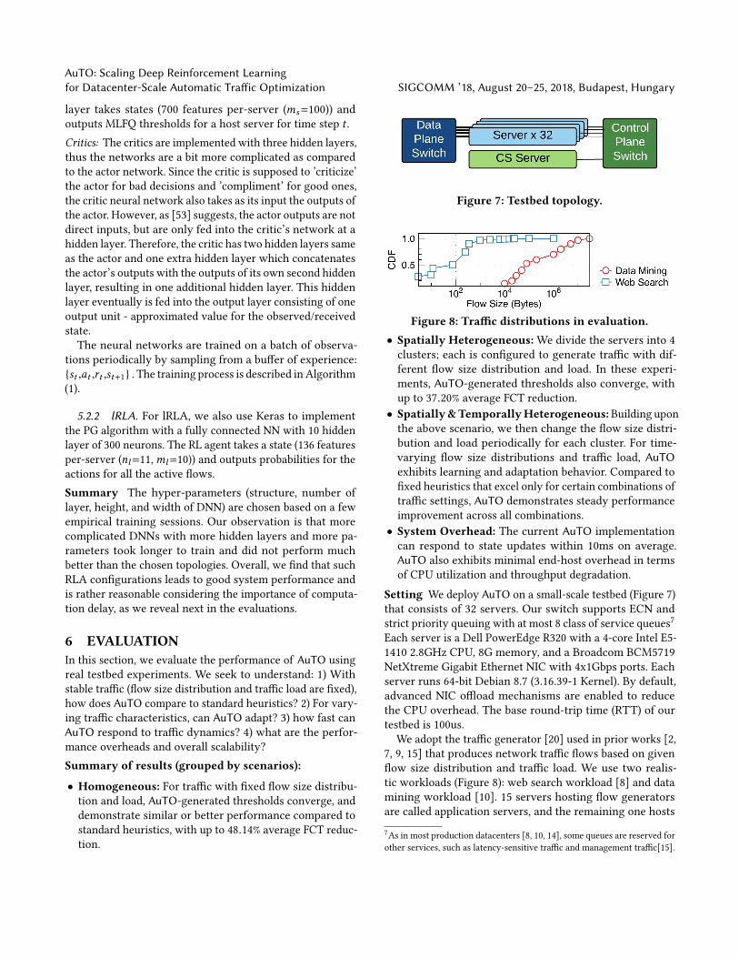
Figure 7: Testbed topology.

Figure 8: Trac distributions in evaluation.• Spatially Heterogeneous:We divide the servers into 4clusters; each is congured to generate trac with dif-ferent ow size distribution and load. In these experi-ments, AuTO-generated thresholds also converge, withup to 37.20% average FCT reduction.• Spatially&TemporallyHeterogeneous:Building uponthe above scenario, we then change the ow size distri-bution and load periodically for each cluster. For time-varying ow size distributions and trac load, AuTOexhibits learning and adaptation behavior. Compared toxed heuristics that excel only for certain combinations oftrac settings, AuTO demonstrates steady performanceimprovement across all combinations.• System Overhead: The current AuTO implementationcan respond to state updates within 10ms on average.AuTO also exhibits minimal end-host overhead in termsof CPU utilization and throughput degradation.

Setting We deploy AuTO on a small-scale testbed (Figure 7)that consists of 32 servers. Our switch supports ECN andstrict priority queuing with at most 8 class of service queues7Each server is a Dell PowerEdge R320 with a 4-core Intel E5-1410 2.8GHz CPU, 8G memory, and a Broadcom BCM5719NetXtreme Gigabit Ethernet NIC with 4x1Gbps ports. Eachserver runs 64-bit Debian 8.7 (3.16.39-1 Kernel). By default,advanced NIC ooad mechanisms are enabled to reducethe CPU overhead. The base round-trip time (RTT) of ourtestbed is 100us.

We adopt the trac generator [20] used in prior works [2,7, 9, 15] that produces network trac ows based on givenow size distribution and trac load. We use two realis-tic workloads (Figure 8): web search workload [8] and datamining workload [10]. 15 servers hosting ow generatorsare called application servers, and the remaining one hosts7As in most production datacenters [8, 10, 14], some queues are reserved forother services, such as latency-sensitive trac and management trac[15].

SIGCOMM ’18, August 20–25, 2018, Budapest, Hungary L. Chen et al.

the CS. Each application server is connected to a data planeswitch using 3 of its ports, as well as to a control plane switchto communicate with the CS server using the remaining port.The 3 ports are congured to dierent subnets, forming 3paths between any pair of application servers. Both switchesare Pronto-3297 48-port Gigabit Ethernet switch. States andactions are sent on the control plane switch (Figure 7).ComparisonTargets We comparewith two popular heuris-tics in ow scheduling: Shortest-Job-First (SJF), and Least-Attained-Service-First (LAS). The main dierence betweenthe two is that SJF schemes [1, 4, 29] require ow size atthe start of a ow, while LAS schemes [8, 14, 43] do not. Forthese algorithms to work, suciently enough data shouldbe collected before calculating their parameters (thresholds).The shortest period to collect enough ow information toform an accurate and reliable ow size distribution is anopen research problem [9, 14, 21, 34], and we note that pre-viously reported distributions are all collected over periodsof at least weeks (Figure 8), which indicates the turn-aroundtime are also at least weeks for these algorithms.In the experiments, we mainly compare with quantized

version of SJF and LAS with 4 priority levels. The prioritylevels are enforced both in the server using Linux qdisc [23]and in the data plane switch using strict priority queue-ing [8]:• Quantized SJF (QSJF):QSJF has three thresholds:α0,α1,α2.We can obtain ow size from the ow generator at itsstart. For ow size s , if x≤α0, it is given highest priority;if x∈(α0,α1], it is given the second priority; and so on. Inthis way, shorter ows are given higher priority, similarto SJF.• Quantized LAS (QLAS):QLAS also has thresholds: β0,β1,β2.All the ows are given high priority at the start. If a owsends more than βi bytes, it is then demoted to the (i+1)-th priority. In this way, longer ows gradually drop tolower priorities.The thresholds for both schemes can be calculated using

methods described in [14] for "type-2/3 ows", and they aredependent on the ow size distribution and trac load. Ineach experiment, unless specied, we use the thresholdscalculated for DCTCP distribution at 80% load (i.e. the totalsending rate is at 80% of the network capacity).

6.1 Experiments6.1.1 Homogeneous traic. In these scenarios, the ow

size distribution and the load generated from all 32 serversare xed.We chooseWeb Search (WS) and Data Mining (DM)distributions at 80% load. These two distributions representdierent group of ows: a mixture of short and long ows(WS) and a set of short ows (DM). The average and 99thpercentile (p99) FCT are shown in Figure 9. We train AuTO

Figure 9: Homogeneous trac: Average and p99 FCT.

Figure 10: Spatially heterogeneous trac: Average andp99 FCT.for 8 hours and use the trained DNNs to schedule ows foranother hour (shown in Figure 9 as AuTO).We make the following observations:• For a mixture of short and long ows (WS), AuTO out-performs the standard heuristics, achieving up to 48.14%average FCT reduction. This is because it can dynamicallychange priority of long ows, avoiding the starvationproblem in the heuristics.• For distribution with mostly short ows (DM), AuTO per-forms similar to the heuristics. Since AuTO also givesany ow highest priority when it starts, AuTO performsalmost the same as QLAS.• Training the RL network results in average FCT reductionof 18.31% and 4.12% for WS&DM distribution respectively,which demonstrates AuTO is capable to learn and adaptto trac characteristics overtime.• We further isolate the incast trac [16] from the collectedtraces, and we nd that they are almost the same withboth QLAS and QSJF. This is because incast behavior isbest handled by the congestion control and parametersetting. DCTCP [3], which is the transport we used inthe experiments, already handles incast very well withappropriate parameter settings [3, 9].

6.1.2 Spatially heterogeneous traic. We proceed to di-vide the servers into 4 clusters to create spatially hetero-geneous trac. We congure the ow generators in eachcluster with dierent distribution and load pairs: <WS, 60%>,<WS, 80%>, <DM, 60%>, <DM, 60%>. We use AuTO to con-trol all 4 clusters, and plot the average and p99 FCTs inFigure 10. For the heuristics, we compute the thresholds for

AuTO: Scaling Deep Reinforcement Learningfor Datacenter-Scale Automatic Traic Optimization SIGCOMM ’18, August 20–25, 2018, Budapest, Hungary

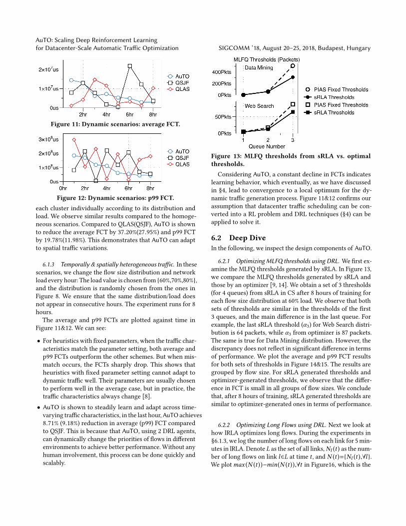
Figure 11: Dynamic scenarios: average FCT.

Figure 12: Dynamic scenarios: p99 FCT.each cluster individually according to its distribution andload. We observe similar results compared to the homoge-neous scenarios. Compared to QLAS(QSJF), AuTO is shownto reduce the average FCT by 37.20%(27.95%) and p99 FCTby 19.78%(11.98%). This demonstrates that AuTO can adaptto spatial trac variations.

6.1.3 Temporally & spatially heterogeneous traic. In thesescenarios, we change the ow size distribution and networkload every hour: The load value is chosen from {60%,70%,80%},and the distribution is randomly chosen from the ones inFigure 8. We ensure that the same distribution/load doesnot appear in consecutive hours. The experiment runs for 8hours.The average and p99 FCTs are plotted against time in

Figure 11&12. We can see:

• For heuristics with xed parameters, when the trac char-acteristics match the parameter setting, both average andp99 FCTs outperform the other schemes. But when mis-match occurs, the FCTs sharply drop. This shows thatheuristics with xed parameter setting cannot adapt todynamic trac well. Their parameters are usually chosento perform well in the average case, but in practice, thetrac characteristics always change [8].• AuTO is shown to steadily learn and adapt across time-varying trac characteristics, in the last hour,AuTO achieves8.71% (9.18%) reduction in average (p99) FCT comparedto QSJF. This is because that AuTO, using 2 DRL agents,can dynamically change the priorities of ows in dierentenvironments to achieve better performance. Without anyhuman involvement, this process can be done quickly andscalably.

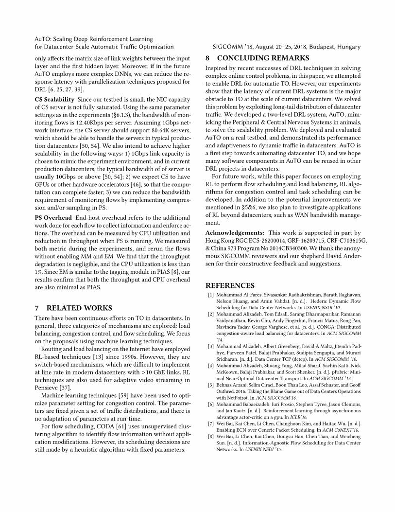
Figure 13: MLFQ thresholds from sRLA vs. optimalthresholds.Considering AuTO, a constant decline in FCTs indicates

learning behavior, which eventually, as we have discussedin §4, lead to convergence to a local optimum for the dy-namic trac generation process. Figure 11&12 conrms ourassumption that datacenter trac scheduling can be con-verted into a RL problem and DRL techniques (§4) can beapplied to solve it.

6.2 Deep DiveIn the following, we inspect the design components of AuTO.

6.2.1 Optimizing MLFQ thresholds using DRL. We rst ex-amine the MLFQ thresholds generated by sRLA. In Figure 13,we compare the MLFQ thresholds generated by sRLA andthose by an optimizer [9, 14]. We obtain a set of 3 thresholds(for 4 queues) from sRLA in CS after 8 hours of training foreach ow size distribution at 60% load. We observe that bothsets of thresholds are similar in the thresholds of the rst3 queues, and the main dierence is in the last queue. Forexample, the last sRLA threshold (α3) for Web Search distri-bution is 64 packets, while α3 from optimizer is 87 packets.The same is true for Data Mining distribution. However, thediscrepancy does not reect in signicant dierence in termsof performance. We plot the average and p99 FCT resultsfor both sets of thresholds in Figure 14&15. The results aregrouped by ow size. For sRLA generated thresholds andoptimizer-generated thresholds, we observe that the dier-ence in FCT is small in all groups of ow sizes. We concludethat, after 8 hours of training, sRLA generated thresholds aresimilar to optimizer-generated ones in terms of performance.

6.2.2 Optimizing Long Flows using DRL. Next we look athow lRLA optimizes long ows. During the experiments in§6.1.3, we log the number of long ows on each link for 5min-utes in lRLA. Denote L as the set of all links,Nl (t ) as the num-ber of long ows on link l∈L at time t , and N (t )={Nl (t ),∀l }.We plotmax (N (t ))−min(N (t )),∀t in Figure16, which is the

SIGCOMM ’18, August 20–25, 2018, Budapest, Hungary L. Chen et al.

Figure 14: Average FCT using MLFQ thresholds fromsRLA vs. optimal thresholds.

Figure 15: p99 FCTusingMLFQThresholds from sRLAvs. optimal thresholds.

Figure 16: Load balancing using lRLA (PG algorithm):dierence in number of long ows on links.dierence in number of long ows on the link that have themost long ows and the link that have the least. This metricis an indicator of load imbalance. We observe that this metricis less than 10 most of the time. When temporary imbal-ance occurs, as shown in the magnied portion of Figure 16(from 24s to 28s), lRLA reacts to the imbalance by routing theexcess ows onto the less congested links. This is because,as we discussed in §2.2, the reward of the PG algorithm isdirectly linked to the throughput: when long ows share alink, the total throughput is less than when they are usingdierent links. lRLA is rewarded when it places long owson dierent links, thus it learns to load balance long ows.

6.2.3 System Overhead. We proceed to investigate theperformance and overheads of AuTOmodules. First, we look

Figure 17: CS response latency: Traces from 4 runs.

Figure 18: CS response latency: Scaling short ows(ms )at the response latency of CS, as well as its scalability. Thenwe examine the overheads of the end-host modules in PS.CS Response Latency During experiments, response delayof the CS server (Figure 17) is measured as follows: tu is thetime instant of CS receiving an update from one server, andts is the time instant of CS sending the action to that server,so the response time is ts−tu . This metric directly shows howfast can the scheduler adapt to trac dynamics reported byPS. We observe that CS can respond to an update within10ms on average for our 32-server testbed. This latency ismainly due to the computation overhead of DNN, as well asthe queueing delay of servers’ updates at CS. AuTO currentlyonly uses CPU. To reduce this latency, one promising direc-tion is CPU-GPU hybrid training and serving [46], whereCPUs handle the interaction with the environment, whileGPUs train the models in the background.Response latency also increases with computation com-

plexity of DNN. In AuTO, the network size is dened by{nl ,ml ,ms }. Since long ows are few, the increment of nl ,mlare expected to be moderate even for datacenters with highload. We increase {nl ,ml } from {11,10} to {1000,1000}, andnd the average response time for lRLA becomes 81.82ms(median 25.14ms). However,ms can increase signicantlyin high load scenarios, and we conduct an experiment tounderstand the impact on response latency of sRLA. In Fig-ure 18, we varyms from 100 (used in the above experiments)to 1000, and measure the response latency. We nd that theaverage response time only slightly increase for largerms .This is because,ms determines the input layer size, which

AuTO: Scaling Deep Reinforcement Learningfor Datacenter-Scale Automatic Traic Optimization SIGCOMM ’18, August 20–25, 2018, Budapest, Hungary

only aects the matrix size of link weights between the inputlayer and the rst hidden layer. Moreover, if in the futureAuTO employs more complex DNNs, we can reduce the re-sponse latency with parallelization techniques proposed forDRL [6, 25, 27, 39].CS Scalability Since our testbed is small, the NIC capacityof CS server is not fully saturated. Using the same parametersettings as in the experiments (§6.1.3), the bandwidth of mon-itoring ows is 12.40Kbps per server. Assuming 1Gbps net-work interface, the CS server should support 80.64K servers,which should be able to handle the servers in typical produc-tion datacenters [50, 54]. We also intend to achieve higherscalability in the following ways: 1) 1Gbps link capacity ischosen to mimic the experiment environment, and in currentproduction datacenters, the typical bandwidth of of server isusually 10Gbps or above [50, 54]; 2) we expect CS to haveGPUs or other hardware accelerators [46], so that the compu-tation can complete faster; 3) we can reduce the bandwidthrequirement of monitoring ows by implementing compres-sion and/or sampling in PS.PS Overhead End-host overhead refers to the additionalwork done for each ow to collect information and enforce ac-tions. The overhead can be measured by CPU utilization andreduction in throughput when PS is running. We measuredboth metric during the experiments, and rerun the owswithout enabling MM and EM. We nd that the throughputdegradation is negligible, and the CPU utilization is less than1%. Since EM is similar to the tagging module in PIAS [8], ourresults conrm that both the throughput and CPU overheadare also minimal as PIAS.

7 RELATEDWORKSThere have been continuous eorts on TO in datacenters. Ingeneral, three categories of mechanisms are explored: loadbalancing, congestion control, and ow scheduling. We focuson the proposals using machine learning techniques.

Routing and load balancing on the Internet have employedRL-based techniques [13] since 1990s. However, they areswitch-based mechanisms, which are dicult to implementat line rate in modern datacenters with >10 GbE links. RLtechniques are also used for adaptive video streaming inPensieve [37].

Machine learning techniques [59] have been used to opti-mize parameter setting for congestion control. The parame-ters are xed given a set of trac distributions, and there isno adaptation of parameters at run-time.For ow scheduling, CODA [61] uses unsupervised clus-

tering algorithm to identify ow information without appli-cation modications. However, its scheduling decisions arestill made by a heuristic algorithm with xed parameters.

8 CONCLUDING REMARKSInspired by recent successes of DRL techniques in solvingcomplex online control problems, in this paper, we attemptedto enable DRL for automatic TO. However, our experimentsshow that the latency of current DRL systems is the majorobstacle to TO at the scale of current datacenters. We solvedthis problem by exploiting long-tail distribution of datacentertrac. We developed a two-level DRL system, AuTO, mim-icking the Peripheral & Central Nervous Systems in animals,to solve the scalability problem. We deployed and evaluatedAuTO on a real testbed, and demonstrated its performanceand adaptiveness to dynamic trac in datacenters. AuTO isa rst step towards automating datacenter TO, and we hopemany software components in AuTO can be reused in otherDRL projects in datacenters.For future work, while this paper focuses on employing

RL to perform ow scheduling and load balancing, RL algo-rithms for congestion control and task scheduling can bedeveloped. In addition to the potential improvements wementioned in §5&6, we also plan to investigate applicationsof RL beyond datacenters, such as WAN bandwidth manage-ment.Acknowledgements: This work is supported in part byHongKong RGCECS-26200014, GRF-16203715, CRF-C703615G,&China 973 ProgramNo.2014CB340300.We thank the anony-mous SIGCOMM reviewers and our shepherd David Ander-sen for their constructive feedback and suggestions.

REFERENCES[1] Mohammad Al-Fares, Sivasankar Radhakrishnan, Barath Raghavan,

Nelson Huang, and Amin Vahdat. [n. d.]. Hedera: Dynamic FlowScheduling for Data Center Networks. In USENIX NSDI ’10.

[2] Mohammad Alizadeh, Tom Edsall, Sarang Dharmapurikar, RamananVaidyanathan, Kevin Chu, Andy Fingerhut, Francis Matus, Rong Pan,Navindra Yadav, George Varghese, et al. [n. d.]. CONGA: Distributedcongestion-aware load balancing for datacenters. In ACM SIGCOMM’14.

[3] Mohammad Alizadeh, Albert Greenberg, David A Maltz, Jitendra Pad-hye, Parveen Patel, Balaji Prabhakar, Sudipta Sengupta, and MurariSridharan. [n. d.]. Data Center TCP (dctcp). In ACM SIGCOMM ’10.

[4] Mohammad Alizadeh, Shuang Yang, Milad Sharif, Sachin Katti, NickMcKeown, Balaji Prabhakar, and Scott Shenker. [n. d.]. pFabric: Mini-mal Near-Optimal Datacenter Transport. In ACM SIGCOMM ’13.

[5] Behnaz Arzani, Selim Ciraci, Boon Thau Loo, Assaf Schuster, and GeoOuthred. 2016. Taking the Blame Game out of Data Centers Operationswith NetPoirot. In ACM SIGCOMM’16.

[6] Mohammad Babaeizadeh, Iuri Frosio, Stephen Tyree, Jason Clemons,and Jan Kautz. [n. d.]. Reinforcement learning through asynchronousadvantage actor-critic on a gpu. In ICLR’16.

[7] Wei Bai, Kai Chen, Li Chen, Changhoon Kim, and Haitao Wu. [n. d.].Enabling ECN over Generic Packet Scheduling. In ACM CoNEXT’16.

[8] Wei Bai, Li Chen, Kai Chen, Dongsu Han, Chen Tian, and WeichengSun. [n. d.]. Information-Agnostic Flow Scheduling for Data CenterNetworks. In USENIX NSDI ’15.

SIGCOMM ’18, August 20–25, 2018, Budapest, Hungary L. Chen et al.

[9] Wei Bai, Li Chen, Kai Chen, Dongsu Han, Chen Tian, and Hao Wang.2017. PIAS: Practical Information-Agnostic Flow Scheduling for Com-modity Data Centers. IEEE/ACM Transactions on Networking (TON)25, 4 (2017), 1954–1967.

[10] Wei Bai, Li Chen, Kai Chen, and Haitao Wu. [n. d.]. Enabling ECN inMulti-Service Multi-Queue Data Centers. In USENIX NSDI ’16.

[11] Theophilus Benson, Aditya Akella, and David Maltz. [n. d.]. NetworkTrac Characteristics of Data Centers in the Wild. In ACM IMC’10.

[12] Shalabh Bhatnagar, Mohammad Ghavamzadeh, Mark Lee, andRichard S Sutton. 2008. Incremental Natural Actor-Critic Algorithms.(2008).

[13] Justin A Boyan, Michael L Littman, et al. 1994. Packet routing indynamically changing networks: A reinforcement learning approach.Advances in neural information processing systems (1994).

[14] Li Chen, Kai Chen, Wei Bai, and Mohammad Alizadeh. [n. d.]. Sched-uling Mix-ows in Commodity Datacenters with Karuna. In ACMSIGCOMM ’16.

[15] Li Chen, Jiacheng Xia, Bairen Yi, and Kai Chen. [n. d.]. PowerMan: AnOut-of-Band Management Network for Datacenters Using Power LineCommunication. In USENIX NSDI’18.

[16] Yanpei Chen, Rean Grith, Junda Liu, Randy H Katz, and Anthony DJoseph. 2009. Understanding TCP incast throughput collapse in dat-acenter networks. The 1st ACM workshop on Research on enterprisenetworking (2009).

[17] Francois Chollet. [n. d.]. Keras Documentation. https://keras.io/. ([n.d.]). (Accessed on 04/18/2017).

[18] Mosharaf Chowdhury and Ion Stoica. [n. d.]. Ecient Coow Sched-uling Without Prior Knowledge. In ACM SIGCOMM ’15.

[19] Mosharaf Chowdhury, Yuan Zhong, and Ion Stoica. [n. d.]. Ecientcoow scheduling with Varys. In ACM SIGCOMM ’14.

[20] Cisco. [n. d.]. Simple client-server application for generat-ing user-dened trac patterns. https://github.com/datacenter/empirical-trac-gen. ([n. d.]). (Accessed on 04/24/2017).

[21] Ralph B Dell, Steve Holleran, and Rajasekhar Ramakrishnan. 2002.Sample size determination. ILAR journal (2002).

[22] Nathan Farrington, George Porter, Sivasankar Radhakrishnan,Hamid Hajabdolali Bazzaz, Vikram Subramanya, Yeshaiahu Fainman,George Papen, and Amin Vahdat. [n. d.]. Helios: A Hybrid Electri-cal/Optical Switch Architecture for Modular Data Centers. In ACMSIGCOMM’10.

[23] Linux Foundation. [n. d.]. Priority qdisc - Linux man page. https://linux.die.net/man/8/tc-prio. ([n. d.]). (Accessed on 04/17/2017).

[24] Python Software Foundation. [n. d.]. Global Interpreter Lock. https://wiki.python.org/moin/GlobalInterpreterLock. ([n. d.]). (Accessed on04/18/2017).

[25] Kevin Frans and Danijar Hafner. 2016. Parallel Trust Region PolicyOptimization with Multiple Actors. (2016).

[26] Albert Greenberg, James R. Hamilton, Navendu Jain, Srikanth Kandula,Changhoon Kim, Parantap Lahiri, David A. Maltz, Parveen Patel, andSudipta Sengupta. [n. d.]. VL2: A Scalable and Flexible Data CenterNetwork. In ACM SIGCOMM’09.

[27] Shixiang Gu, Ethan Holly, Timothy Lillicrap, and Sergey Levine. [n.d.]. Deep reinforcement learning for robotic manipulation with asyn-chronous o-policy updates. In Proceedings of Robotics and Automation(ICRA), 2017 IEEE International Conference on.

[28] W. K. Hastings. 1970. Biometrika (1970). http://www.jstor.org/stable/2334940

[29] Chi-Yao Hong, Matthew Caesar, and P Godfrey. [n. d.]. Finishing owsquickly with preemptive scheduling. In ACM SIGCOMM ’12.

[30] C. Hopps. 2000. Analysis of an Equal-Cost Multi-Path Algorithm. RFC2992 (2000).

[31] Kurt Hornik. [n. d.]. Approximation Capabilities of Multilayer Feed-forward Networks. Neural Netw., 1991 ([n. d.]).

[32] Shuihai Hu, Kai Chen, Haitao Wu, Wei Bai, Chang Lan, Hao Wang,Hongze Zhao, and Chuanxiong Guo. 2016. Explicit path control in com-modity data centers: Design and applications. IEEE/ACM Transactionson Networking (2016).

[33] Srikanth Kandula, Sudipta Sengupta, Albert Greenberg, Parveen Pa-tel, and Ronnie Chaiken. [n. d.]. The Nature of Datacenter Trac:Measurements and Analysis. In ACM IMC’09.

[34] Russell V Lenth. 2001. Some practical guidelines for eective samplesize determination. The American Statistician (2001).

[35] Timothy P. Lillicrap, Jonathan J. Hunt, Alexander Pritzel, Nicolas Heess,Tom Erez, Yuval Tassa, David Silver, and Daan Wierstra. 2015. Contin-uous control with deep reinforcement learning. CoRR abs/1509.02971(2015). arXiv:1509.02971 http://arxiv.org/abs/1509.02971

[36] Hongzi Mao, Mohammad Alizadeh, Ishai Menache, and Srikanth Kan-dula. [n. d.]. ResourceManagementwithDeep Reinforcement Learning.In ACM HotNets ’16.

[37] Hongzi Mao, Ravi Netravali, and Mohammad Alizadeh. [n. d.]. NeuralAdaptive Video Streaming with Pensieve. In ACM SIGCOMM ’17.

[38] N. McKeown, T. Anderson, H. Balakrishnan, G. Parulkar, L. Peter-son, J. Rexford, S. Shenker, and J. Turner. 2008. OpenFlow: Enablinginnovation in campus networks. ACM CCR (2008).

[39] Volodymyr Mnih, Adria Puigdomenech Badia, Mehdi Mirza, AlexGraves, Timothy Lillicrap, Tim Harley, David Silver, and KorayKavukcuoglu. [n. d.]. Asynchronous methods for deep reinforcementlearning. In ICML’16.

[40] Volodymyr Mnih, Koray Kavukcuoglu, David Silver, Alex Graves, Ioan-nis Antonoglou, Daan Wierstra, and Martin Riedmiller. 2013. Playingatari with deep reinforcement learning. arXiv preprint arXiv:1312.5602(2013).

[41] Volodymyr Mnih, Koray Kavukcuoglu, David Silver, Alex Graves, Ioan-nis Antonoglou, Daan Wierstra, and Martin Riedmiller. 2013. Playingatari with deep reinforcement learning. arXiv preprint arXiv:1312.5602(2013).

[42] Philipp Moritz, Robert Nishihara, Stephanie Wang, Alexey Tumanov,Richard Liaw, Eric Liang,William Paul, Michael I Jordan, and Ion Stoica.2017. Ray: A Distributed Framework for Emerging AI Applications.arXiv preprint arXiv:1712.05889 (2017).

[43] Ali Munir, Ihsan A Qazi, Zartash A Uzmi, Aisha Mushtaq, Saad NIsmail, M Safdar Iqbal, and Basma Khan. [n. d.]. Minimizing owcompletion times in data centers. In IEEE INFOCOM ’13.

[44] Netlter.Org. [n. d.]. The netlter.org project. https://www.netlter.org/. ([n. d.]). (Accessed on 04/17/2017).

[45] NVIDIA. [n. d.]. Deep Learning Frameworks. https://developer.nvidia.com/deep-learning-frameworks. ([n. d.]). (Accessed on 04/18/2017).

[46] NVlabs. [n. d.]. Hybrid CPU/GPU implementation of the A3C algo-rithm for deep reinforcement learning. https://github.com/NVlabs/GA3C. ([n. d.]). (Accessed on 06/13/2018).

[47] OpenAI. [n. d.]. OpenAI Gym. https://gym.openai.com/. ([n. d.]).(Accessed on 04/24/2017).

[48] Adam Paszke, Sam Gross, Soumith Chintala, and Gregory Chanan.2017. Pytorch. (2017).

[49] Yang Peng, Kai Chen, Guohui Wang, Wei Bai, Ma Zhiqiang, and Lin Gu.[n. d.]. HadoopWatch: A First Step Towards Comprehensive TracForcecasting in Cloud Computing. In IEEE INCOCOM ’14.

[50] Arjun Roy, Hongyi Zeng, Jasmeet Bagga, George Porter, and Alex CSnoeren. [n. d.]. Inside the Social Network’s (Datacenter) Network. InACM SIGCOMM’15.

[51] John Schulman, Sergey Levine, Philipp Moritz, Michael I. Jordan, andPieter Abbeel. 2015. Trust Region Policy Optimization. CoRR (2015).

AuTO: Scaling Deep Reinforcement Learningfor Datacenter-Scale Automatic Traic Optimization SIGCOMM ’18, August 20–25, 2018, Budapest, Hungary

[52] David Silver, Aja Huang, Chris J Maddison, Arthur Guez, Laurent Sifre,George Van Den Driessche, Julian Schrittwieser, Ioannis Antonoglou,Veda Panneershelvam, Marc Lanctot, et al. 2016. Mastering the gameof Go with deep neural networks and tree search. Nature (2016).

[53] David Silver, Guy Lever, Nicolas Heess, Thomas Degris, DaanWierstra,andMartin Riedmiller. 2014. Deterministic Policy Gradient Algorithms.In Proceedings of the 31st International Conference on InternationalConference on Machine Learning - Volume 32 (ICML’14). JMLR.org,I–387–I–395. http://dl.acm.org/citation.cfm?id=3044805.3044850

[54] Arjun Singh, Joon Ong, Amit Agarwal, Glen Anderson, Ashby Armis-tead, Roy Bannon, Seb Boving, Gaurav Desai, Bob Felderman, PaulieGermano, et al. [n. d.]. Jupiter Rising: A Decade of Clos Topologiesand Centralized Control in Google’s Datacenter Network. In ACMSIGCOMM’15.

[55] Richard S. Sutton and Andrew G. Barto. 1998. Introduction to Rein-forcement Learning.

[56] Richard S Sutton, David A. McAllester, Satinder P. Singh, and YishayMansour. 2012. Policy Gradient Methods for Reinforcement Learningwith Function Approximation. (2012).

[57] TensorFlow. [n. d.]. API Documentation: TensorFlow. https://www.tensorow.org/api_docs/. ([n. d.]). (Accessed on 04/18/2017).

[58] Matt Welsh, David Culler, and Eric Brewer. [n. d.]. SEDA: An Ar-chitecture for Well-conditioned, Scalable Internet Services. In SOSP’01.

[59] Keith Winstein and Hari Balakrishnan. [n. d.]. Tcp ex machina:Computer-generated congestion control. In ACM SIGCOMM ’13.

[60] Neeraja J. Yadwadkar, Ganesh Ananthanarayanan, and Randy Katz. [n.d.]. Wrangler: Predictable and Faster Jobs Using Fewer Resources. InSOCC ’14.

[61] Hong Zhang, Li Chen, Bairen Yi, Kai Chen, Mosharaf Chowdhury, andYanhui Geng. [n. d.]. CODA: Toward automatically identifying andscheduling coows in the dark. In ACM SIGCOMM ’16.