Optimization via Search

CPSC 315 – Programming Studio

Spring 2008

Project 2, Lecture 4

Adapted from slides of Yoonsuck Choe

Improving Results and Optimization

Assume a state with many variables Assume some function that you want to

maximize/minimize the value of Searching entire space is too complicated

Can’t evaluate every possible combination of variables

Function might be difficult to evaluate analytically

Iterative improvement

Start with a complete valid state Gradually work to improve to better and

better states Sometimes, try to achieve an optimum, though

not always possible Sometimes states are discrete, sometimes

continuous

Simple Example

One dimension (typically use more):

x

functionvalue

Simple Example

Start at a valid state, try to maximize

x

functionvalue

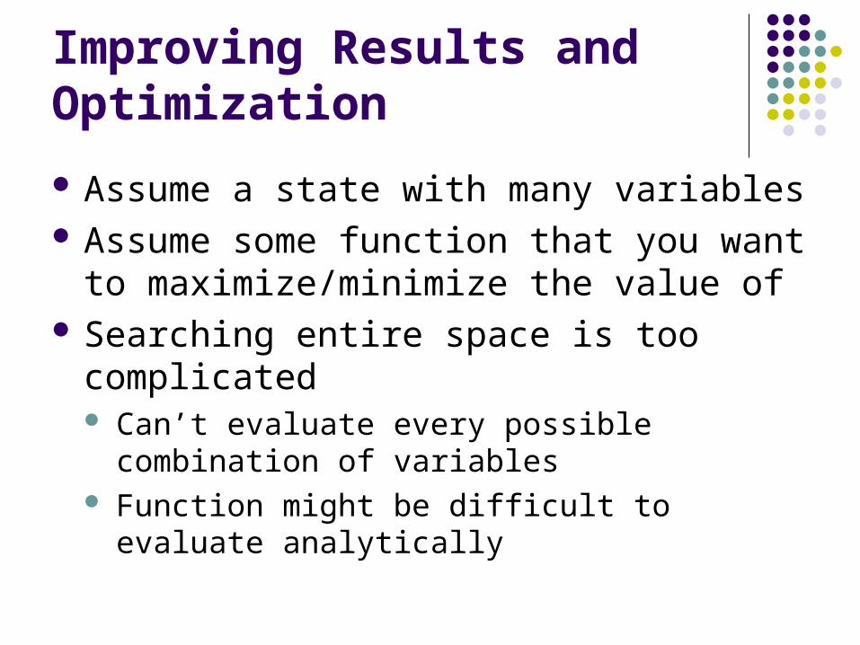
Simple Example

Move to better state

x

functionvalue

Simple Example

Try to find maximum

x

functionvalue

Hill-Climbing

Choose Random Starting State

Repeat

From current state, generate n random

steps in random directions

Choose the one that gives the best new

value

While some new better state found

(i.e. exit if none of the n steps were better)

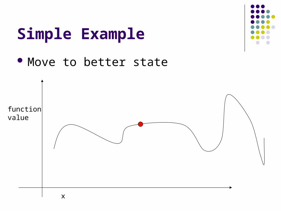
Simple Example

Random Starting Point

x

functionvalue

Simple Example

Three random steps

x

functionvalue

Simple Example

Choose Best One for new position

x

functionvalue

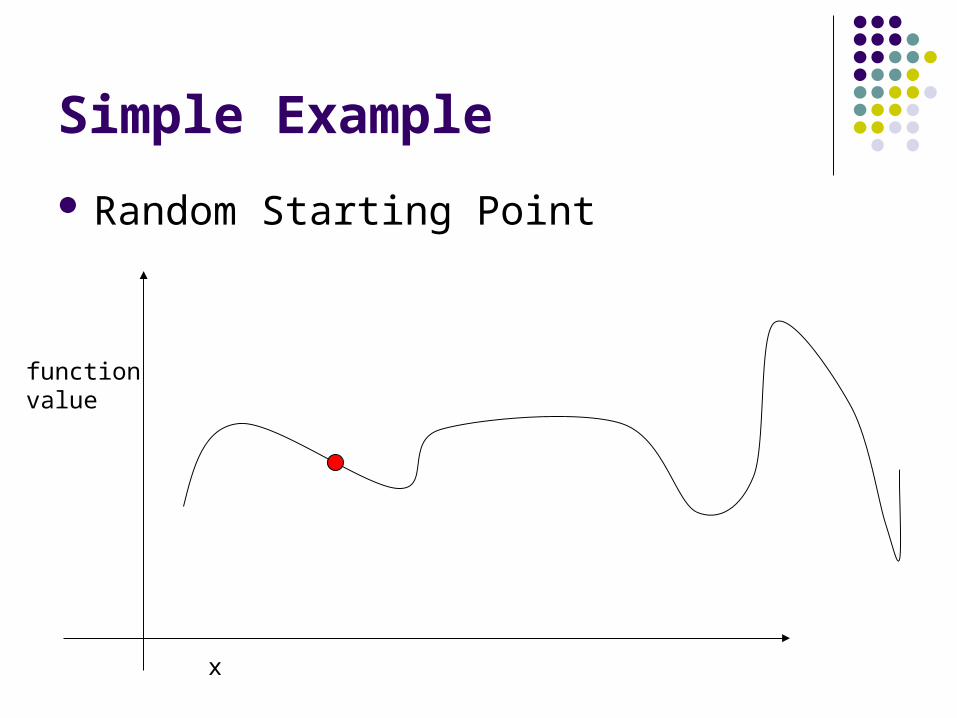
Simple Example

Repeat

x

functionvalue

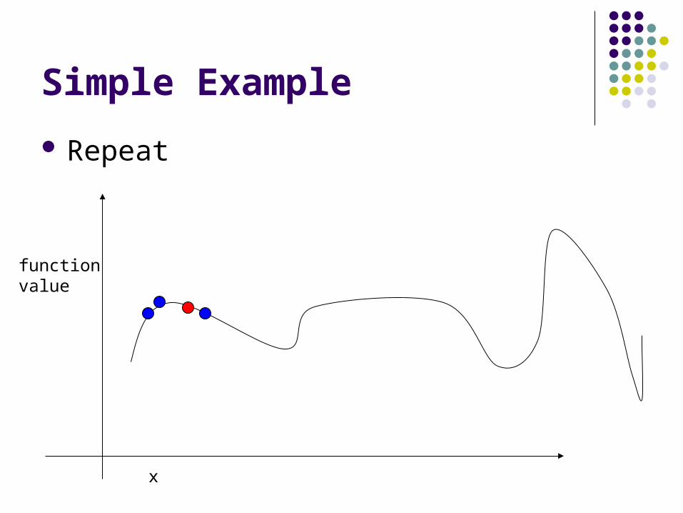
Simple Example

Repeat

x

functionvalue

Simple Example

Repeat

x

functionvalue

Simple Example

Repeat

x

functionvalue

Simple Example

No Improvement, so stop.

x

functionvalue

Problems With Hill Climbing

Random Steps are Wasteful Addressed by other methods

Local maxima, plateaus, ridges Can try random restart locations Can keep the n best choices (this is also called “beam

search”)

Comparing to game trees: Basically looks at some number of available next moves

and chooses the one that looks the best at the moment Beam search: follow only the best-looking n moves

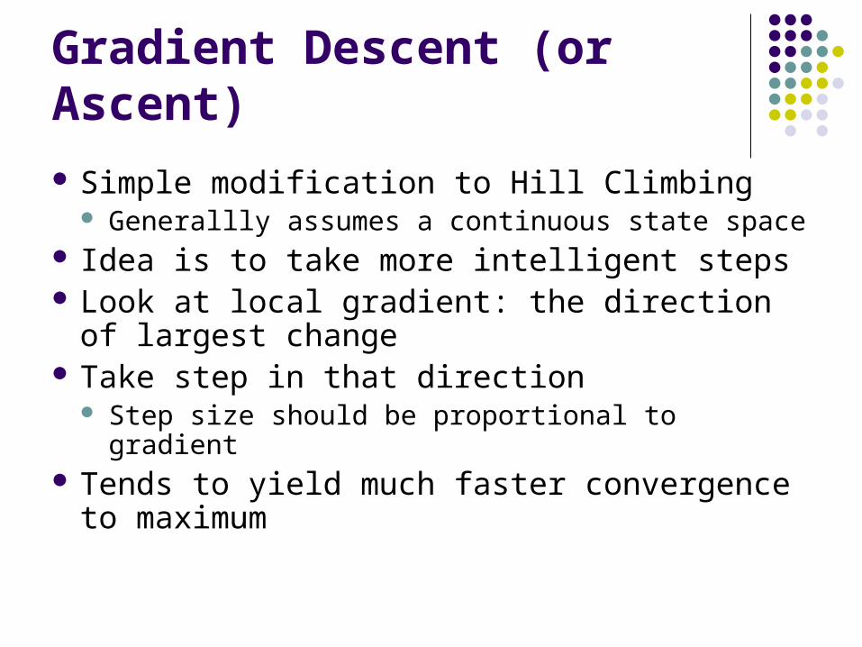
Gradient Descent (or Ascent)

Simple modification to Hill Climbing Generallly assumes a continuous state space

Idea is to take more intelligent steps Look at local gradient: the direction of largest

change Take step in that direction

Step size should be proportional to gradient Tends to yield much faster convergence to

maximum

Gradient Ascent

Random Starting Point

x

functionvalue

Gradient Ascent

Take step in direction of largest increase

(obvious in 1D, must be computed

in higher dimensions)

x

functionvalue

Gradient Ascent

Repeat

x

functionvalue

Gradient Ascent

Next step is actually lower, so stop

x

functionvalue

Gradient Ascent

Could reduce step size to “hone in”

x

functionvalue

Gradient Ascent

Converge to (local) maximum

x

functionvalue

Dealing with Local Minima

Can use various modifications of hill climbing and gradient descent Random starting positions – choose one Random steps when maximum reached Conjugate Gradient Descent/Ascent

Choose gradient direction – look for max in that direction

Then from that point go in a different direction

Simulated Annealing

Simulated Annealing

Annealing: heat up metal and let cool to make harder By heating, you give atoms freedom to move

around Cooling “hardens” the metal in a stronger state

Idea is like hill-climbing, but you can take steps down as well as up. The probability of allowing “down” steps goes

down with time

Simulated Annealing

Heuristic/goal/fitness function E (energy) Generate a move (randomly) and compute

E = Enew-Eold

If E <= 0, then accept the move If E > 0, accept the move with probability:

Set

T is “Temperature”

kT

E

eEP

)(

Simulated Annealing

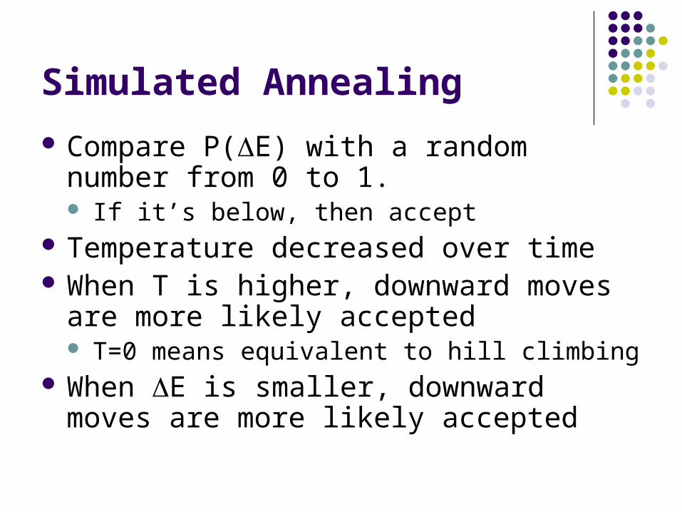
Compare P(E) with a random number from 0 to 1. If it’s below, then accept

Temperature decreased over time When T is higher, downward moves are more

likely accepted T=0 means equivalent to hill climbing

When E is smaller, downward moves are more likely accepted

“Cooling Schedule”

Speed at which temperature is reduced has an effect

Too fast and the optima are not found Too slow and time is wasted

Simulated Annealing

Random Starting Point

x

functionvalue

T = Very High

Simulated Annealing

Random Step

x

functionvalue

T = Very High

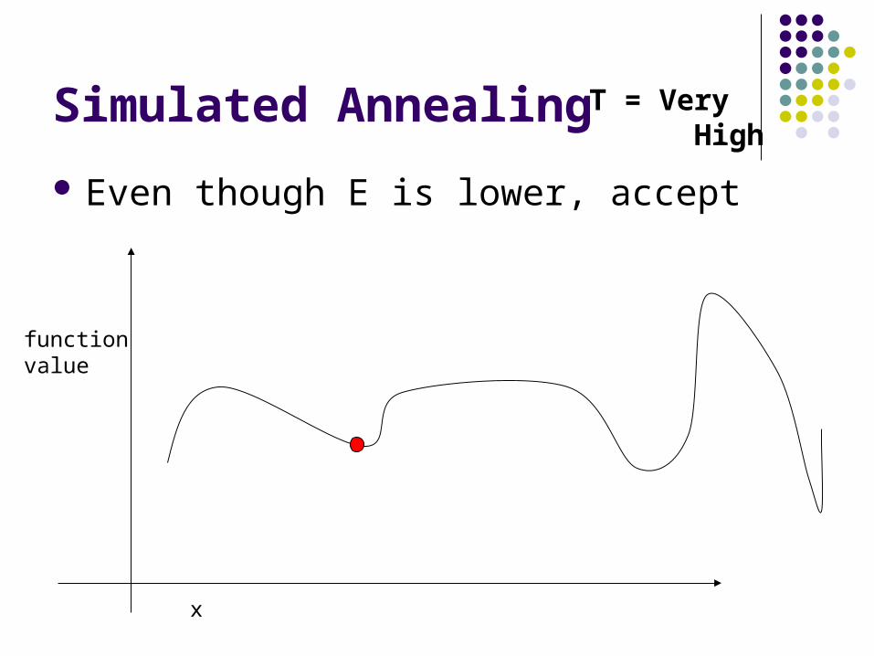
Simulated Annealing

Even though E is lower, accept

x

functionvalue

T = Very High

Simulated Annealing

Next Step; accept since higher E

x

functionvalue

T = Very High

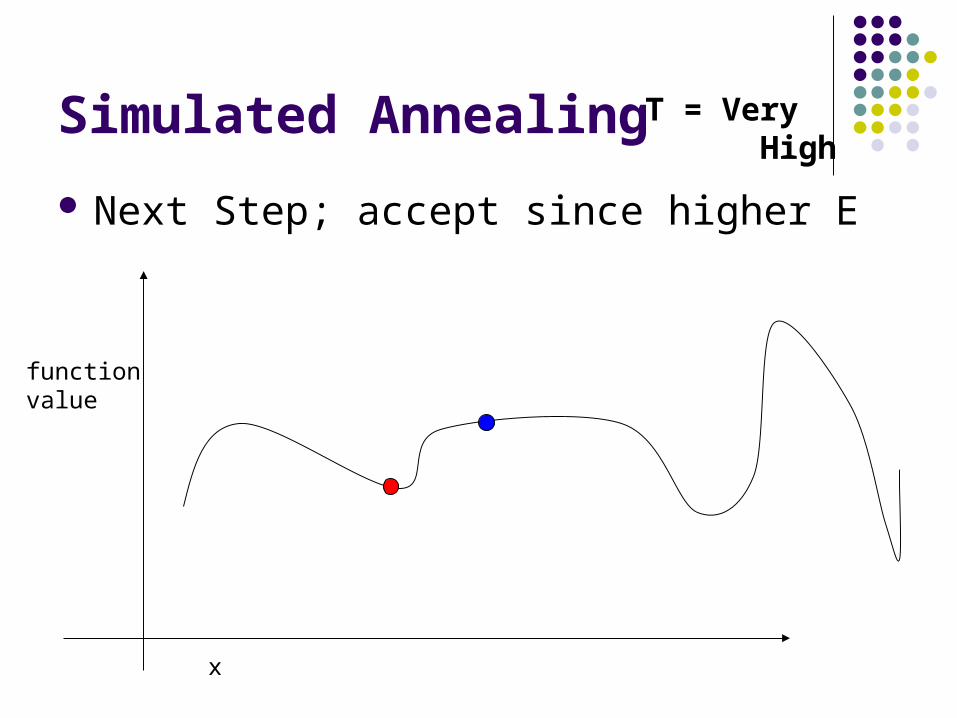
Simulated Annealing

Next Step; accept since higher E

x

functionvalue

T = Very High

Simulated Annealing

Next Step; accept even though lower

x

functionvalue

T = High

Simulated Annealing

Next Step; accept even though lower

x

functionvalue

T = High

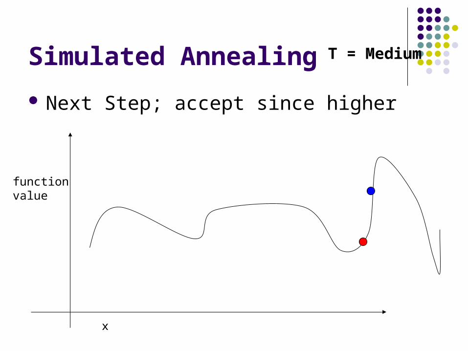
Simulated Annealing

Next Step; accept since higher

x

functionvalue

T = Medium

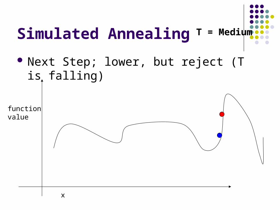
Simulated Annealing

Next Step; lower, but reject (T is falling)

x

functionvalue

T = Medium

Simulated Annealing

Next Step; Accept since E is higher

x

functionvalue

T = Medium

Simulated Annealing

Next Step; Accept since E change small

x

functionvalue

T = Low

Simulated Annealing

Next Step; Accept since E larget

x

functionvalue

T = Low

Simulated Annealing

Next Step; Reject since E lower and T low

x

functionvalue

T = Low

Simulated Annealing

Eventually converge to Maximum

x

functionvalue

T = Low

Other Optimization Approach: Genetic Algorithms

State = “Chromosome” Genes are the variables

Optimization Function = “Fitness” Create “Generations” of solutions

A set of several valid solution

Most fit solutions carry on Generate next generation by:

Mutating genes of previous generation “Breeding” – Pick two (or more) “parents” and create

children by combining their genes