OPTIMIZATION OF MISSION DESIGN FOR CONSTRAINED …
153
OPTIMIZATION OF MISSION DESIGN FOR CONSTRAINED LIBRATION POINT SPACE MISSIONS A DISSERTATION SUBMITTED TO THE DEPARTMENT OF AERONAUTICS AND ASTRONAUTICS AND THE COMMITTEE ON GRADUATE STUDIES OF STANFORD UNIVERSITY IN PARTIAL FULFILLMENT OF THE REQUIREMENTS FOR THE DEGREE OF DOCTOR OF PHILOSOPHY Samantha I. Infeld December 2005 Revision Date: December 16, 2005
Transcript of OPTIMIZATION OF MISSION DESIGN FOR CONSTRAINED …

OPTIMIZATION OF MISSION DESIGN FOR CONSTRAINED
LIBRATION POINT SPACE MISSIONS
A DISSERTATION
SUBMITTED TO THE DEPARTMENT OF
AERONAUTICS AND ASTRONAUTICS
AND THE COMMITTEE ON GRADUATE STUDIES
OF STANFORD UNIVERSITY
IN PARTIAL FULFILLMENT OF THE REQUIREMENTS
FOR THE DEGREE OF
DOCTOR OF PHILOSOPHY
Samantha I. Infeld
December 2005
Revision Date: December 16, 2005

Copyright c© 2006 by Samantha I. Infeld
All Rights Reserved
ii

I certify that I have read this dissertation and that, in myopinion, it is fully adequate in scope and quality as a disser-tation for the degree of Doctor of Philosophy.
Walter Murray(Principal Advisor)
I certify that I have read this dissertation and that, in myopinion, it is fully adequate in scope and quality as a disser-tation for the degree of Doctor of Philosophy.
Christopher Cassell
I certify that I have read this dissertation and that, in myopinion, it is fully adequate in scope and quality as a disser-tation for the degree of Doctor of Philosophy.
Sanjay Lall
I certify that I have read this dissertation and that, in myopinion, it is fully adequate in scope and quality as a disser-tation for the degree of Doctor of Philosophy.
Per Enge
Approved for the University Committee on Graduate Studies:
iii

iv

Abstract
Designing space missions to remain in the vicinity of an equilibrium point in a three-
body system is both useful and more difficult than for a two-body system. Earth orbits
are the most common two-body trajectory (the spacecraft being the second body). In
a three-body system we are considering a spacecraft near two large masses rotating
around their center of mass.
Because of the rotation of the system, there is not just one point of equilibrium, but
rather five points where the gravitational and centripetal accelerations exactly cancel;
three where the satellite is collinear with the other masses and two points where the
satellite forms in-plane equilateral triangles with the other masses. These points are
called libration points (L1-L5), or Lagrange points since it was Lagrange who obtained
the first solutions of the three-body problem. This work chooses the Earth-Sun L2 point
at which to apply the developed mission design approach because of current proposals
for telescope missions at that point, but is equally applicable to any libration point in
any three-body system.
The chosen point is behind the Earth from the Sun and is useful for a telescope mis-
sion because it is outside Earth’s atmosphere and magnetosphere (beyond the moon’s
orbit), but close enough for fast communications and possibly human maintenance mis-
sions. Also the telescope can point away from the light and heat interference of the
Sun, Earth, and Moon simultaneously. The collinear points (L1-L3,) although useful
locations, are unstable equilibriums[1], which makes trajectories near them quite sensi-
tive to differences in velocity or force perturbations by the full space environment (e.g.
solar radiation pressure).
Trajectory and control history design about the unstable Sun-Earth L2 point will
become increasingly complex as additional mechanical and scheduling constraints ac-
company scientific observation missions. Satisfying such constraints in designing a
station-keeping plan may be viewed as an optimization problem, with the objective
of maximizing the mission goals. It then adds little further complexity to minimize fuel
usage as part of the objective, which is always a goal in space mission planning. Solving
this design problem is an illustration of the power and ease of this alternative multiple-
body mission design approach, which is based on optimization of the whole trajectory
and control design. In this thesis, the formulation of such an optimization problem is
explained in several steps using increasingly complex dynamical and mission constraint
v

models, and some resulting solutions for these steps are presented and discussed. The
continuous time problem is first discretized using a pseudospectral method, and the re-
sulting finite dimensional problem is solved using a sequential quadratic programming
algorithm. This approach is implemented by the software package DIDO, which calls
the sparse nonlinear optimization software SNOPT. The design approach is discussed as
a general mission optimization process, which can easily be used further into the design
process and for more types of missions than the examples here, by applying it to a more
realistically modeled and more highly constrained libration-point mission design.
vi

Acknowledgments
Acknowledgments go here.
vii

viii

Contents
List of Tables, Figures, and Algorithms xi
1 Introduction 1
1.1 Preliminary Investigation . . . . . . . . . . . . . . . . . . . . . . . . . . 5
1.2 Thesis Outline . . . . . . . . . . . . . . . . . . . . . . . . . . . . . . . . 7
2 Libration Point Missions 9
2.1 The Three Body Problem . . . . . . . . . . . . . . . . . . . . . . . . . . 10
2.2 Past Mission Trajectory Design and Control . . . . . . . . . . . . . . . . 13
2.3 Optimization in Mission Design . . . . . . . . . . . . . . . . . . . . . . . 18
2.4 Mission Design Optimal Control Problem . . . . . . . . . . . . . . . . . 19
2.4.1 Basic Formulation . . . . . . . . . . . . . . . . . . . . . . . . . . 20
2.4.2 Complex Formulations . . . . . . . . . . . . . . . . . . . . . . . . 24
3 Solving the Optimal Control Problem 31
3.1 Discretization of the Optimal Control Problem . . . . . . . . . . . . . . 32
3.1.1 Experiments with simple finite differencing and user differentiation 33
3.1.2 Direct Collocation Method . . . . . . . . . . . . . . . . . . . . . 34
3.1.3 Pseudospectral Method . . . . . . . . . . . . . . . . . . . . . . . 37
3.2 Solution of the Discretized Problem. . . . . . . . . . . . . . . . . . . . . 40
3.2.1 Nonlinear Programming Problem . . . . . . . . . . . . . . . . . . 40
3.2.2 Algorithm Details . . . . . . . . . . . . . . . . . . . . . . . . . . 40
3.2.3 Implementation Analysis . . . . . . . . . . . . . . . . . . . . . . 41
4 Results for an Example Mission 43
4.1 Mission-Unconstrained Results . . . . . . . . . . . . . . . . . . . . . . . 44
4.1.1 Simple Model Definition . . . . . . . . . . . . . . . . . . . . . . . 44
4.1.2 Simple Model Solutions . . . . . . . . . . . . . . . . . . . . . . . 44
4.1.3 Perturbed Model Definition . . . . . . . . . . . . . . . . . . . . . 61
4.1.4 Perturbed Model Solutions . . . . . . . . . . . . . . . . . . . . . 61
4.2 Mission Constrained Results . . . . . . . . . . . . . . . . . . . . . . . . . 73
4.2.1 Attitude Constraint Definition . . . . . . . . . . . . . . . . . . . 73
4.2.2 Perturbed Mission Constrained Model Solutions . . . . . . . . . 74
ix

4.3 Comparison with Reference Orbit Approach . . . . . . . . . . . . . . . . 93
5 Multiple Spacecraft: A Second Example Mission 97
5.1 General Framework . . . . . . . . . . . . . . . . . . . . . . . . . . . . . . 99
5.2 Libration Point Formations . . . . . . . . . . . . . . . . . . . . . . . . . 103
5.3 Numerical Examples . . . . . . . . . . . . . . . . . . . . . . . . . . . . . 105
5.4 Framework for Spacecraft Formations . . . . . . . . . . . . . . . . . . . 114
6 Conclusions and Future Work 129
Bibliography 130
x

Tables, Figures, and Algorithms
Tables
2.1 Mission Models (Sections of Results, Ch.4) . . . . . . . . . . . . . . . . 20
3.1 Limitations of direct collocation method . . . . . . . . . . . . . . . . . . 37
3.2 Submatrix diagonal in D matrix for N = 4 . . . . . . . . . . . . . . . . . 39
4.1 Summary of Results: Simple Model . . . . . . . . . . . . . . . . . . . . . 56
4.2 Summary of Results: Perturbed Model. tf in TU, Cost in DU/TU and
m/s . . . . . . . . . . . . . . . . . . . . . . . . . . . . . . . . . . . . . . 72
4.3 Summary of Results: Constrained/Unconstrained Comparison. Cost in
DU/TU . . . . . . . . . . . . . . . . . . . . . . . . . . . . . . . . . . . . 93
Figures
2.1 Coordinate system for the restricted three-body problem . . . . . . . . . 11
2.2 Past and Planned Libration Point Missions . . . . . . . . . . . . . . . . 14
2.3 Lissajous reference orbit for Genesis mission[22] . . . . . . . . . . . . . . 16
2.4 Halo orbit from early JWST planning.[23] Note size in comparison to
Moon’s orbit around Earth. . . . . . . . . . . . . . . . . . . . . . . . . . 17
2.5 The thrust direction u must stay out of the sun-view cone. . . . . . . . 26
4.1 Simple Model Example 1: An Optimal Trajectory for Large Halo Input 46
4.2 Simple Model Example 1: Thrust over time . . . . . . . . . . . . . 47
4.3 Simple Model Example 1: Evolution of the Hamiltonian; note the
scale on the ordinate . . . . . . . . . . . . . . . . . . . . . . . . . . . . . 48
4.4 Simple Model Example 1: Comparison of the velocity states to those
propagated by ODE45 in Matlab (dotted) . . . . . . . . . . . . . . . . . 49
4.5 Simple Model Example 2: An Optimal Trajectory for Small Halo
Input, df = D . . . . . . . . . . . . . . . . . . . . . . . . . . . . . . . . . 51
4.6 Simple Model Example 2: A 2-D Zoomed View of the Optimal Tra-
jectory . . . . . . . . . . . . . . . . . . . . . . . . . . . . . . . . . . . . . 52
4.7 Simple Model Example 2: Thrust over time . . . . . . . . . . . . . 52
xi

4.8 Simple Model Example 3: An Optimal Trajectory for Small Halo
Input, df = D/2 . . . . . . . . . . . . . . . . . . . . . . . . . . . . . . . 53
4.9 Simple Model Example 3: A 2-D Zoomed View of the Optimal Tra-
jectory . . . . . . . . . . . . . . . . . . . . . . . . . . . . . . . . . . . . . 54
4.10 Simple Model Example 3: Thrust over time . . . . . . . . . . . . . 55
4.11 Simple Model Example 4: An Optimal Trajectory for Full Halo Orbit
Input, df = D/2 . . . . . . . . . . . . . . . . . . . . . . . . . . . . . . . 57
4.12 Simple Model Example 4: A Zoomed View of the Optimal Trajectory,
df = D/2 . . . . . . . . . . . . . . . . . . . . . . . . . . . . . . . . . . . 58
4.13 Simple Model Example 5: An Optimal Trajectory for Stationary L2
Input, df = D . . . . . . . . . . . . . . . . . . . . . . . . . . . . . . . . . 59
4.14 Simple Model Example 5: Thrust over time . . . . . . . . . . . . . 59
4.15 Speed and Accuracy vs Number of Nodes . . . . . . . . . . . . . . . . . 60
4.16 Perturbed Model Example 1: Optimal trajectory with no bounds on
states . . . . . . . . . . . . . . . . . . . . . . . . . . . . . . . . . . . . . 62
4.17 Perturbed Model Example 1: Optimal trajectory with no bounds on
states (zoomed) . . . . . . . . . . . . . . . . . . . . . . . . . . . . . . . . 63
4.18 Perturbed Model Example 1: Thrust over time with no bounds on
states . . . . . . . . . . . . . . . . . . . . . . . . . . . . . . . . . . . . . 64
4.19 Perturbed Model Example 2: Optimal trajectory with initial states
bound . . . . . . . . . . . . . . . . . . . . . . . . . . . . . . . . . . . . . 65
4.20 Perturbed Model Example 2: Thrust over time with initial states
bound . . . . . . . . . . . . . . . . . . . . . . . . . . . . . . . . . . . . . 66
4.21 Perturbed Model Example 3: Optimal trajectory with states bound 67
4.22 Perturbed Model Example 3: Thrust over time with states bound . 68
4.23 Perturbed Model Example 4: Optimal trajectory with states bound 69
4.24 Perturbed Model Example 4: Thrust over time with states bound . 70
4.25 Perturbed Model Example 5: Optimal trajectory with states bound 71
4.26 Perturbed Model Example 5: Thrust over time with states bound . 72
4.27 The thrust direction (defined by the control vector) must stay out of the
sun-view cone. . . . . . . . . . . . . . . . . . . . . . . . . . . . . . . . . 73
4.28 Constrained Example 1: Optimal trajectory with attitude constraint
and states not bound . . . . . . . . . . . . . . . . . . . . . . . . . . . . . 75
4.29 Constrained Example 1: Thrust over time with attitude constraint
and states not bound . . . . . . . . . . . . . . . . . . . . . . . . . . . . . 76
4.30 Constrained Example 1: Attitude over time w/out constraint and
states not bound . . . . . . . . . . . . . . . . . . . . . . . . . . . . . . . 76
xii

4.31 Constrained Example 1: Attitude over time with constraint and states
not bound . . . . . . . . . . . . . . . . . . . . . . . . . . . . . . . . . . . 77
4.32 Constrained Example 2: Optimal trajectory with constraint and ini-
tial states bound . . . . . . . . . . . . . . . . . . . . . . . . . . . . . . . 78
4.33 Constrained Example 2: Thrust over time with attitude constraint
and initial states bound . . . . . . . . . . . . . . . . . . . . . . . . . . . 79
4.34 Constrained Example 2: Attitude over time w/out constraint but
initial states bound . . . . . . . . . . . . . . . . . . . . . . . . . . . . . . 79
4.35 Constrained Example 2: Attitude over time with constraint and initial
states bound . . . . . . . . . . . . . . . . . . . . . . . . . . . . . . . . . 80
4.36 Constrained Example 2: Optimal trajectory with constraint and ini-
tial states bound, twice as many nodes . . . . . . . . . . . . . . . . . . . 81
4.37 Constrained Example 2: Optimal trajectory with constraint and ini-
tial states bound, twice as many nodes (zoomed) . . . . . . . . . . . . . 82
4.38 Constrained Example 2: Thrust over time with constraint and initial
states bound, twice as many nodes . . . . . . . . . . . . . . . . . . . . . 83
4.39 Constrained Example 2: Attitude over time with constraint and initial
states bound, twice as many nodes . . . . . . . . . . . . . . . . . . . . . 83
4.40 Constrained Example 3: Optimal trajectory with constraint and states
bound . . . . . . . . . . . . . . . . . . . . . . . . . . . . . . . . . . . . . 84
4.41 Constrained Example 3: Thrust over time with constraint and states
bound . . . . . . . . . . . . . . . . . . . . . . . . . . . . . . . . . . . . . 85
4.42 Constrained Example 3: Attitude over time w/out constraint but
states bound . . . . . . . . . . . . . . . . . . . . . . . . . . . . . . . . . 85
4.43 Constrained Example 3: Attitude over time with constraint and states
bound . . . . . . . . . . . . . . . . . . . . . . . . . . . . . . . . . . . . . 86
4.44 Constrained Example 4: Optimal trajectory with constraint and states
bound . . . . . . . . . . . . . . . . . . . . . . . . . . . . . . . . . . . . . 87
4.45 Constrained Example 4: Thrust over time with constraint and states
bound . . . . . . . . . . . . . . . . . . . . . . . . . . . . . . . . . . . . . 88
4.46 Constrained Example 4: Attitude over time w/out constraint but
states bound . . . . . . . . . . . . . . . . . . . . . . . . . . . . . . . . . 88
4.47 Constrained Example 4: Attitude over time with constraint and states
bound . . . . . . . . . . . . . . . . . . . . . . . . . . . . . . . . . . . . . 89
4.48 Constrained Example 5: Optimal trajectory with constraint and states
bound . . . . . . . . . . . . . . . . . . . . . . . . . . . . . . . . . . . . . 90
xiii

4.49 Constrained Example 5: Thrust over time with constraint and states
bound . . . . . . . . . . . . . . . . . . . . . . . . . . . . . . . . . . . . . 91
4.50 Constrained Example 5: Attitude over time w/out constraint but
states bound . . . . . . . . . . . . . . . . . . . . . . . . . . . . . . . . . 91
4.51 Constrained Example 5: Attitude over time with constraint and states
bound . . . . . . . . . . . . . . . . . . . . . . . . . . . . . . . . . . . . . 92
4.52 Reference Orbit Approach: Near-Optimal Trajectory . . . . . . . . 94
4.53 Reference Orbit Approach: Thrust over time . . . . . . . . . . . . . 95
4.54 Reference Orbit Approach: Attitude over time . . . . . . . . . . . . 95
4.55 Reference Orbit Approach: Error in x position state variable . . . . 96
5.1 Trajectories for a two-agent DSS . . . . . . . . . . . . . . . . . . . . . . 107
5.2 Separation between the two spacecraft over time . . . . . . . . . . . . . 108
5.3 Relative orbit for the two-agent DSS . . . . . . . . . . . . . . . . . . . . 109
5.4 Thrust along the x axis for the two-agent DSS . . . . . . . . . . . . . . 110
5.5 Evolution of the Hamiltonian for the two-agent DSS; note the scale on
the ordinate . . . . . . . . . . . . . . . . . . . . . . . . . . . . . . . . . . 111
5.6 Comparison of the position states of spacecraft one (solid) to those prop-
agated by ODE45 in Matlab (dotted) . . . . . . . . . . . . . . . . . . . . 112
5.7 Trajectories for a two-agent DSS with periodicity constraints . . . . . . 113
5.8 Input and Optimal Trajectories for a two-agent DSS with periodicity
constraints. NOT TO SCALE: stretched to show orbit shape . . . . . . 114
5.9 Trajectories on the y-z plane for a two-agent DSS with periodicity con-
straints. NOT TO SCALE: stretched along the y axis . . . . . . . . . . 115
5.10 Thrust along the x axis for the periodic two-agent DSS. . . . . . . . . . 115
5.11 Separation between the two spacecraft over time . . . . . . . . . . . . . 116
5.12 Relative orbit for the periodic two-agent DSS . . . . . . . . . . . . . . . 117
5.13 The values of the position half of xi(t0) and xi(tf ) for i = 1, 2 are marked
with circles on this close-up view of the trajectory where it starts and
ends. . . . . . . . . . . . . . . . . . . . . . . . . . . . . . . . . . . . . . 118
5.14 The values of the velocity half xi(t0) and xi(tf ) for i = 1 are marked
with circles on this close-up view of the velocity trajectory start and end. 119
5.15 Evolution of the Hamiltonian for the periodic two-agent DSS . . . . . . 120
5.16 Comparison of the position states of spacecraft one (solid) to those prop-
agated by ODE45 in Matlab(dotted) . . . . . . . . . . . . . . . . . . . . 121
5.17 Trajectories for a large-baseline two-agent DSS . . . . . . . . . . . . . . 122
xiv

5.18 Thrust along the x axis for the large-baseline two-agent DSS; note the
scale on the ordinate . . . . . . . . . . . . . . . . . . . . . . . . . . . . . 123
5.19 Separation between the two spacecraft over time . . . . . . . . . . . . . 124
5.20 Relative orbit for the large-baseline two-agent DSS . . . . . . . . . . . . 125
5.21 Evolution of the Hamiltonian for the large-baseline two-agent DSS; note
the scale on the ordinate . . . . . . . . . . . . . . . . . . . . . . . . . . . 126
5.22 Comparison of the position states of spacecraft one (solid) to those prop-
agated by ODE45 in Matlab (dotted) . . . . . . . . . . . . . . . . . . . . 127
xv

xvi

Chapter 1
Introduction
The problem of mission design for a spacecraft at the Sun-Earth L2 point has been
studied and accomplished in past missions. Farquhar first explored trajectory design
strategies in the regions of libration points, taking into account periodic disturbances,
eccentricity correction, gravitational perturbations and solar radiation pressure.[2] In
these recent libration point missions, the spacecraft describes a Lissajous path about
the libration point, which is usually corrected by engine burns at the crossing of the
Earth-Sun line to ensure that the spacecraft will not escape the vicinity in the next few
orbits. (A Lissajous path, named after the nineteenth century mathematician, is defined
as the path of a point each of whose coordinates is under not necessarily related harmonic
motion, so it stays within a certain area over time but does not repeat its path.) Several
methods to compute trajectory control strategies have been developed, for example the
Target Point Method[3], and the Floquet Mode method[4], which incorporates the idea
of invariant manifold tubes from dynamical systems theory. This type of mission design,
taking advantage of these tubes associated with libration point orbits, was used on the
recent Genesis mission[5]. These methods target a trajectory control strategy based on
a good estimate from the theory of an orbit that remains about the libration point only
in a simple model, and they may optimize maneuvers individually from this strategy.
They do not optimize the design because they do not search the whole acceptable
design space. These missions do not require that the spacecraft remain in some specific
orbit that exists only with a simple theoretical model, but the recent design methods
do not consider acceptable paths other than the reference orbit. This outside space
of alternate paths then are very likely to contain a path with a lower associated fuel
expenditure, when considering a more accurate modeling of the forces and errors. Thus,
the approach presented here will necessarily result in mission designs with lower fuel
costs than mission designs based on reference orbits (as well as being a simpler and
more direct design approach).
Future missions will carry more complicated and sensitive spacecraft structure and
on-board instruments, and consequently will require more constraints on the station-
keeping plan. As an example, consider the problem of an astronomical mission during
1

2 Chapter 1 Introduction
which the cryogenic optics must be pointed away from the Sun, such as the James Webb
Telescope or the Terrestrial Planet Finder. Such constraints limit the thrust direction.
To keep light away from the instrument side of the spacecraft, there must be a large sun
shield, and the spacecraft must be oriented such that the shield is completely protecting
the instruments. Any blast of light (visible and IR) from the Sun, Earth, or Moon will
destroy the cryogenic instrument, and even infrared radiated from the spacecraft will
overwhelm the very faint astronomical signals. This sun shield will produce extra forces
and torques due to the solar radiation pressure on the surface area of the shield[6].
The Earth-Sun L2 point provides a location where the sources of heat are all coming
from the same general direction, and is far enough from the Earth to avoid major at-
mospheric and electrical field interference, but close enough to avoid the large antenna
power requirements of interplanetary missions.
Proposals of more highly constrained missions necessitates the ability to create mis-
sion design plans that not only keep the spacecraft in the libration points vicinity, but
also optimize for minimum fuel usage and other mission goals (e.g. least interference
with scientific goals). The design approach presented in this thesis introduces an alter-
native direction in the development of more sophisticated processes for space mission
design. The direction is that of concurrent engineering to incorporate optimization
from the beginning of the design process, resulting in lower fuel requirements because of
elimination of unnecessary assumptions about the orbit or control design (fuel-burning
maneuvers to maintain planned orbit). In fact, other design approaches which make
these assumptions, and design the trajectory and control design in series are unable to
find fuel-optimal designs. Further, a concurrent design approach that does take the en-
tire mission design process as one optimal control problem as is done here, but without
taking advantage of sophisticated numerical methods, also leads to unsolvable problems.
The design of a control plan and corresponding trajectory (which together we call
the ‘mission design’) is posed here as a single optimization problem that finds the
optimum maneuver schedule to minimize fuel, achieve or maximize mission goals, and
meet the mechanical and scheduling constraints. This optimization problem would be
recognized from the controls point of view as an optimal control problem, which simply
means we are searching for a control vector that when applied to a dynamical system
results in optimum behavior as modeled by an objective function[7]. Optimizing the
design of a space mission almost always implies minimizing fuel use. This minimizes the
percentage of the spacecraft’s mass taken by fuel, and maximizes the mass available for
operations equipment. In the work presented here, it has been assumed that minimizing
fuel use is the primary goal. We do not necessarily propose to control a particular orbit
shape in minimum fuel; rather, we propose that the more fundamental problem is to

3
explore the mission-length trajectory design space (e.g. by varying initial estimates
as the optimization algorithm’s starting point) to find minimum-fuel solutions. Thus
it is part of the method to find many locally optimal solutions, rather than looking
for the one local optimal solution closest to an estimate of a particular orbit shape.
These solutions can then be evaluated for use in specific missions by adding appropriate
position, attitude, and timing constraints and using the solutions as starting points for
another iteration of the optimization algorithm. This approach, of telling an object
what to do, rather than how to do it, has been successfully applied for the design and
control of a variety of Earth-orbiting formations[8, 9] and libration-point formations
[10]. This thesis looks briefly at formations, but the approach is mostly applied to a
single spacecraft system design space with no restrictions on the orbit shape. The first
step uses a simple force model. The optimal trajectories found in this space have zero
cost (no fuel use needed), and are therefore global optimizers. Then some perturbations
and mission constraints are added to the problem formulation. The next step in the
development of this method is to iterate these trajectories in a design space with a
complex (full) force model, to get an accurate minimum fuel solution for the set of
chosen constraints.
This systems engineering approach of concurrently choosing the orbit and satisfying
the mission constraints; concurrent design and optimization; results in ease of applica-
tion. It is easy, and trivial to the solving of the problem, to change mission constraints,
spacecraft or force models, or even location of the mission, because these are all simple
inputs into a single encompassing optimization problem. This is a flexible approach
in that the search space for minimum-fuel trajectories is not confined to be close to
a reference orbit. Rather, the algorithm can search any combination of positions, ve-
locities, and thrust at each time step, with the equations of motion in the region as a
feasibility requirement rather than a requirement at each step in the algorithm, and the
characteristics of the orbit restricted only by this feasibility through the laws of physics
and a requirement that the spacecraft not have drifted too far by the end of the mission
lifetime. The example mission used here illustrates how the concurrent approach opens
the design space to allow total mission optimization, and the ease of altering the details
of the problem formulation in order to guide the mission design process. This ease in
formulation translates to use of this approach for any type of space mission design.
The mission design problem approached in this way is a single optimal control prob-
lem; a dynamic system that is affected by some chosen ‘controls’ is solved for it’s behav-
ior over a time period to find the set of controls that minimize a particular measure of
the ‘cost’ of the behavior [11, 7]. The controls in this case are the accelerations added
to spacecraft from burning the engines, where the magnitude and direction over time

4 Chapter 1 Introduction
are the ‘control variables’ that are free to be chosen. The first formulation of any opti-
mal control problem involves equations describing the dynamics of the system, the cost
to be minimized, and any constraints which must be met to consider a solution valid.
If the variables in these equations are continuous functions (e.g. an object’s position
over time), the number of variables being considered in the optimal control problem is
infinite, since each continuous variable is actually a variable at all points in time, an
infinite set. Optimal control problems can rarely be solved analytically, which implies
that we need to use numerical methods. The first step is to discretize the problem,
which is to define the system at discrete points rather than with continuous functions.
This results in a finite number of variables because the system variables are only defined
at the discrete points. The number of variables for the optimal control problem is then
the number of variables in the system times the number of discretization points. The
consequence of discretizing the optimal control problem explored here is a nonlinearly
constrained optimization problem. The unstable dynamics of the L2 vicinity require
a more accurate representation of the trajectory to solve the problem than two-body
mission design problems. Because the paths are not simple to describe mathematically
and similar paths can diverge enormously over the long timescale of these mission, the
grid representing the position, velocity (state variables), and added acceleration (control
variables) at a finite number of time values in the discretized problem must be very fine
or very well-designed to enable a numerical solution.
Methods of optimizing mission design using existing commercial software packages
work well enough for libration point mission design optimization if the design is sequen-
tial; first finding a reference trajectory that will work and then optimizing the maneuver
(controls) history to maintain this given constraints and perturbations. Using the con-
current trajectory control design and open design space described above, the standard
methods would result in a discrete problem too large computationally to be of use during
a mission, and may not even be solvable.
There is interest in spacecraft formation missions at libration points, which would
multiply the computational workload with standard methods, but is greatly reduced in
computation time and formulation complexity using the method introduced here (see
Chapter 4). In this work, once the concurrent design problem framework is set up,
the optimal control problem is solved by a Legendre pseudospectral method[12, 13, 14].
The entire Legendre pseudospectral procedure is automated in a Matlab code called
DIDO[15] that is fully integrated with SNOPT[16], a sparse nonlinear programming
solver through the Tomlab[17] interface.

1.1 Preliminary Investigation 5
1.1 Preliminary Investigation
This trajectory and control design problem is a hard problem because of the unstable
dynamics of the region. It is a place of balance of large forces, which means that paths
are very sensitive to perturbations. Small addition accelerations do not cause a constant
or even slowly growing offset from the original path, they cause a very different new
path. This is due to the unstable nature of the equilibrium of forces at the libration
point. When the system is modeled with point masses and circular orbits, there exist
paths that look like orbits because they are periodic in all axes; some forming a repeating
round path around the line connecting the bodies and the libration point. These orbits
exist because of the equilibrium nature of the vicinity. With any added complexity to the
force model, these paths diverge from periodic and become an orbit about one of the two
bodies within an orbit or two. In practice it takes a relatively small added acceleration
(thrust from the a spacecraft’s engine) to return to a similar path, if it is added at
just the right place and direction. To find a path, looking beyond just correcting to
these theoretical ‘orbits’, in which the required additional forces are a minimum (a fuel-
optimal path) is even harder because changing the path a small amount to conduct the
search may change the fuel required by a large amount, again due to the sensitivity of
the problem.
Solar radiation pressure imposes a significant force on a spacecraft with a large
surface area, such as a solar shield, and thus will impact the control plan as the force
varies with the spacecrafts attitude. The attitude for a scientific observation mission is
determined at most times by the object of observation. During maneuvers, the attitude
is determined by the direction of thrust required. As described earlier, the direction is
limited for these types of missions to keep the instruments from pointing too close to
the Sun. The constraint on the attitude then is both very important and an increase in
complexity of the problem. As this consideration along with mission requirements on
the allowable timing of maneuvers will tend to increase the fuel needed, optimization of
fuel use becomes even more important.
The Astrogator and Visualization Option tools, in the Satellite Tool Kit[18], were
used for a preliminary investigation of the effect of solar radiation pressure on a space-
craft with large surface area in a traditional halo orbit within a complex model of all
forces. Given a non-divergent orbit about L2, with the addition of a changing force along
the Sun-Earth-L2 line, showed that the orbit diverges from the vicinity as a result. This
confirmed the large influence of the solar radiation pressure on the spacecrafts sensitive
trajectory about L2. Experimentation with a much simpler model in Matlab illustrated
the useful but non-intuitive influence of the exact magnitude and timing of one impulse

6 Chapter 1 Introduction
on the total ∆v needed to keep the trajectory from diverging in the next orbit[19].
This preliminary work confirmed that the mechanics of the spacecraft and the con-
straints of the mission easily cause stationkeeping complications. It also showed that
decreasing the fuel usage was possible with the burn schedule as control variables, while
still satisfying constraints. This justified the further work of posing the mission planning
as an optimization problem.
The next preliminary work was to find a method of discretizing the continuous op-
timization problem to form the matrices describing the cost and constraint functions at
discrete points that are input into the optimization routine. The discretization method
must capture the complex dynamics of the problem well enough with as few total vari-
ables as possible. With a simple, equal-length timestep discretization, the optimization
problem could not be solved. The discrete problem was too inaccurate for all the con-
straints describing the motion to hold, and the optimization routine could not find a
feasible point.
Another commonly used discretization method, direct collocation, implemented with
the use of commercial software, worked with this optimization problem in situations too
limited for this design approach. Optimal trajectories and control plans were found
when the number of timesteps was below fifty, which limited the mission length to
about one year, and when the input (guess) trajectory was very close to an optimal
trajectory. This requires too much preparation work before the design optimization
begins, while also limiting the design space to designs already known, as the optimal
trajectories necessarily stay close to the input near-optimal trajectories.
The pseudospectral discretization method was chosen because it required a relatively
smaller discretized problem in order to capture enough of the complex dynamics. It was
found to provide a discrete formulation for which the optimization routine could find
solutions, given correct scaling of the problem, for any type of input trajectory and
control plan, not just those close to a known optimal trajectory. This method then is
used for all the results presented in Chapter 4 and 5. All the discretization methods
explored, and the optimization method, are described in Chapter 3.

1.2 Thesis Outline 7
1.2 Thesis Outline
The problem formulation is described at the end of Chapter 2, first in general and
then its specific form when applied to a libration point space mission. This follows the
Chapter 2 discussion of libration point missions including the framework for mission
design and past approaches to designing these missions.
The methods used to solve the mission design optimization problem once it is for-
mulated are presented in Chapter 3. The choice of a direct method to solve the optimal
control problem is discussed. As direct methods first discretize the problem and then
apply an optimization algorithm, the choice of these methods are discussed, and those
implemented are further described.
The results of applying this approach to an example libration point mission are
presented in Chapter 4. A brief comparison to the reference orbit approach follows five
examples of specific problem formulations and solutions. The examples are repeated
two more times after proving the expected results in the case of a simple gravitational
model with no mission constraints, to show the effect of adding perturbations to the
model and mission constraints to the problem formulation.
The ability to apply this to a second libration mission example is explored in Chapter
5. Here the problem of libration point spacecraft formation is solved using this mission
design optimization approach for a few different sets of mission requirements.
Conclusions and possibilities expanding this approach to mission design in the future
are found in Chapter 6.

8

Chapter 2
Libration Point
Missions
This chapter first introduces the dynamical space in which libration point space
missions are designed. Then past work on libration mission design is described, together
with a summary of the methods used to compute the trajectories. This includes how
optimization has been used during the design process for libration point missions. Prior
to the work here, optimization had not been used for overall design. A review of
traditional methods of incorporating optimization into space mission design in general
is presented.
Space missions are designed in a multi-body space for several reasons. Traditionally,
interplanetary trajectories were designed as patched conic paths. This means the trajec-
tory is divided into several arcs during which only two bodies at a time are considered.
This method is a very good approximation for most type of interplanetary missions, and
can be used until the very final stages of planning. However, more time or fuel efficient
trajectory options can be produced by considering all the bodies simultaneously, and
these savings can make a difference for a spacecraft using low-thrust engines or visiting
several moons of a planet. The rotation of bodies in the solar system produces dynam-
ics that are observed in the multi-body space and can be taken advantage of to find
very efficient paths for transferring between bodies or for stationing at a place near but
not orbiting a body. These efficient paths can be seen as moving through or remaining
near libration points. Libration points are where the gravitational forces of two massive
bodies are exactly balanced with the centripetal force needed to rotate with them about
the collective center of mass of the system, such that a third body of negligible mass
could remain at that point in the rotating system. (Note: these equilibrium points are
only static given the assumption of circular orbits of the masses.) Libration point mis-
sions are those that take advantage of the local dynamics to spend some or all of their
mission in the vicinity of such a point. The advantage to this location for a spacecraft
is to be close to a planet without having to orbit it. This can be used for a research,
construction, or communication station for example at an Earth-Moon libration point
9

10 Chapter 2 Libration Point Missions
because it is an easy transfer to orbit either body. A data-relay satellite at Earth-Moon
L2 was proposed in 1966 and considered for Apollo 17. It can also be useful for scientific
observation missions. Libration points are far enough away from the bodies to which
they belong to have full perspective of their surface, and be outside atmospheric and
magnetic influence on the instruments. This lack of interference also results in clearer
astronomical observations. The most popular type of libration point mission currently
being planned is astronomical observation at the Sun-Earth libration point that remains
on the dark side of the Earth. This location makes it easy to block the radiation from
the Earth, Moon, and Sun at once, while staying in relatively easy communication range
and is close enough to allow maintenance.
Preliminary design work for a libration point mission is done in the context of the
circular restricted three-body problem, as that is the framework in which the libration
points are stationary. This problem is described below, and illustrated for the Sun-
Earth-spacecraft case.
2.1 The Three Body Problem
The circular restricted three-body problem (CR3BP) is defined as a system of two
bodies in circular orbits about their barycenter, and a third body of negligible mass.
The equations of motion are solved for the third body. The stationary solutions of this
problem are the five libration points. The equations are most simply and therefore most
often expressed in the rotating barycentric frame (as they will be here). In this frame,
the barycenter of the two masses is the origin. The x axis is the line through the center
of the two large bodies. The frame rotates about the z axis with the angular velocity
ω of the two large bodies about each other. This angular velocity is then 2π radians
divided by the period of the two mass system. The two bodies here are the Sun and
the Earth, so the period is one year.
The equations of motion for this problem are derived in many places, for example
Battin’s astrodynamics textbook [1], but is derived here for completeness and to estab-
lish terminology. With the goal of expressing the acceleration of the third body, we
start by taking the second derivative with respect to time (in the inertial frame) of the
position vector of the third body, ~r.
~r/I = ~r + ~ω × r + ~ω × (~ω × ~r) + 2~ω × ~r + ~rB.
The vector ~rB is the position vector with respect to the body frame, whose origin
is at the center of the third body in the three-body system. Since the point whose
motion we wish to know is the center of the third body, the position vector has zero

2.1 The Three Body Problem 11
Figure 2.1 Coordinate system for the restricted three-body problem
length since it points from the origin of the body frame to the point in question (i.e.
the same point). In evaluating this equation, we note then that ~rB = 0. We also have
~ω = 0 because of the circular orbit assumption. It is important to be clear that the
derivatives of ~r are with respect to the rotating barycentric frame since ~r is defined
in that frame. Eventually, we want an expression for the acceleration of the position
vector with respect to the rotating barycentric frame, so that we can describe the third
body’s motion in this frame. Since the angular velocity is about the z axis, the cross
products with ω have simple expressions as seen in the following simplification of the
above equation.
~r/I = ~r − ω2(xi + yj) + 2ω(yi − xj). (2.1)
We know the acceleration of the position vector in the inertial frame, ~r/I , because
it is the acceleration on any point in the system due to the gravity of the two large
bodies. The force potential at a certain point due to the gravity of body 1 is µ1/r1p in
the direction of body 1, where µ1 = Gm1, and r1p is the distance between body 1 and
the point p; G is the universal gravitation constant, and m1 is the mass of body 1. We
can express ~r/I as the gradient of the total gravitational force potential. First define ~r13
as the vector from body 1 to body 3 (the third body whose motion we are deriving),
with the plain r13 as the distance between the bodies. The same holds for body 2. Now
we can write
~r/I = ∇(−µ1
r13~r13 −
µ2
r23~r23). (2.2)
Combining (2.1) and (2.2) gives

12 Chapter 2 Libration Point Missions
~r − ω2(xi + yj) + 2ω(yi − xj) = ∇(−µ1
r13~r13 −
µ2
r23~r23).
Separating this equation into the components x,y,z, in the rotating frame gives
x − ω2x − 2ωy =∂
∂x(−
µ1
r13~r13 −
µ2
r23~r23)
y − ω2y + 2ωx =∂
∂y(−
µ1
r13~r13 −
µ2
r23~r23)
z =∂
∂z(−
µ1
r13~r13 −
µ2
r23~r23).
Since r13 =√
(x − r1)2 + y2 + z2 and r23 =√
(x + r2)2 + y2 + z2, where rj is the
distance from the origin (barycenter) to body j, evaluating the differentiation on the
right hand sides gives the equations of motion,
x − ω2x − 2ωy = −µ1(x − r1)
r313
−µ2(x + r2)
r323
(2.3)
y − ω2y + 2ωx = −µ1y
r313
−µ2y
r323
(2.4)
z = −µ1z
r313
−µ2z
r323
. (2.5)
The non-dimensional units chosen here are TU for time units, DU for distance units,
and MU for mass units, ω = 1 radian/TU, m1 +m2 = 1 MU , and r12 = 1 DU. Defining
unsubscripted µ as the mass ratio, equal to m2
m1+m2in any units (2 is always the smaller
mass), then in nondimensional units body 1 is also µ DU from the origin and body 2 is
1 − µ DU from the origin.
In nondimensional units, r13 and r23 are
r13 =√
(x − µ)2 + y2 + z2 and r23 =√
(x + 1 − µ)2 + y2 + z2.
Evaluating the partial differentials in (2.3-2.5) using the above definitions gives the
nondimensional equations of motion,

2.2 Past Mission Trajectory Design and Control 13
x − 2y − x = −(1 − µ)(x − µ)
r313
−µ(x + 1 − µ)
r323
y + 2x − y = −(1 − µ)y
r313
−µy
r323
z = −(1 − µ)z
r313
−µz
r323
.
When using the equations of motion to design a spacecraft trajectory, we must
include the force of the engine burning fuel. We may also include other forces that per-
turb the simplified three-body system, such as solar radiation pressure and the moon’s
gravity (without rewriting the equations in terms of a 4-body problem). All of these
outside forces are incorporated in the variable F to finally express the acceleration of
the spacecraft (third body) in each direction as follows:
x = 2y + x −(1 − µ)(x − µ)
r313
−µ(x + 1 − µ)
r323
+ Fx/m (2.6)
y = −2x + y −(1 − µ)y
r313
−µy
r323
+ Fy/m (2.7)
z = −(1 − µ)z
r313
−µz
r323
+ Fz/m, (2.8)
where Fi is the component of the sum of the outside forces along the ith axis, and m is
the current mass of the spacecraft.
2.2 Past Mission Trajectory Design and Control
The equations of motion described above are solved for a control plan (component
of F applied with the engine as a function on time), and the resulting trajectory (x, y, z
position as functions of time), within defined mission constraints. This is the solution
to the mission design problem. The work presented here is an approach to solving the
mission design problem that takes into account the difficulty of solving the problem in
the unstable dynamics of a multi-body system, and the desired complexity of mission
constraints for future space missions. Therefore, this approach is elaborated and applied
in the context of a constrained libration point space mission, using a particular mission
currently in the planning stages as a reference for spacecraft model and constraints. Fol-
lowing is an overview of past libration point mission planning work, with more attention
paid to the mission used as a reference. These spacecraft were all put in Lissajous paths

14 Chapter 2 Libration Point Missions
Figure 2.2 Past and Planned Libration Point Missions
(coordinates under harmonic motion) with matching periods in the x and y coordinates
(sometimes called ‘quasi-periodic’ as they fill a torus). Some had preliminary designs
as ‘halo’ orbits, which are Lissajous paths for which the x and y period align with the z
period to form a perfectly periodic orbit. Halo orbits are solutions to the CR3BP (and
do not exist without velocity corrections in more complex models), which can only be
found with large enough amplitudes in the x and y coordinates and correct choice of z
amplitude such that the resulting period matches the x and y periods. The amplitudes
and periods resulting in a halo orbit in the CR3BP cannot be found analytically, but
must be computed numerically.[20]
Several space missions have been accomplished at the Sun-Earth L1 point to study
the Sun (Earth study at this point has been designed but not yet completed). There
is currently one mission at the Sun-Earth L2 point, and most current proposals also
choose this point. The International Sun-Earth Explorer (ISEE-3) and Solar Heliosphere
Observatory (SOHO) were launched into large halo orbits about L1 in 1978 and 1996
respectively. ISEE-3 went into orbit around L2 in 1983 to study cosmic rays. The
actual cost of maintaining the orbit were reduced from 7.5 meters/second per year for

2.2 Past Mission Trajectory Design and Control 15
ISEE-3 to 2.3 meters/second per year for SOHO [21]. This is because ISEE-3 was
controlled to exactly maintain the halo orbit using thrust along all axes, while SOHO
used thrust only in the x direction as it crossed the x-z plane about every 90 days,
resulting in a Lissajous trajectory that approximated the nominal halo orbit. It was
found that not having a precise halo orbit did not affect common types of mission
design requirements motivated by the scientific mission goals. The solar wind observer
WIND was stationed both at L1 in a Lissajous orbit starting in 1995. The Advanced
Composition Explorer (ACE) was put into a small Lissajous orbit about L1 in 1997,
and the Microwave Anisotropy Probe (MAP) was placed into a small Lissajous about
L2 in 2001. Map performs station-keeping maneuvers about every 3 months. Genesis,
a solar sample return mission, went into a large Lissajous orbit about L1 in 2001. The
James Webb Space Telescope (JWST) will be put into a large Lissajous orbit about
L2. All of these trajectories were designed with a process of a preliminary reference
orbit based on the circular restricted three-body problem, and then used various means
to use this as a guess for a more complex numerical calculation of the trajectory and
the required control scheme to add velocity with engine maneuvers to maintain the
reference trajectory calculated with the simple model. Other steps at this point were
designing the transfer trajectory from Earth to the long-term halo or Lissajous orbit,
and calculating the extra velocity needed for ‘station-keeping’, i.e. correcting for errors
in position measurement or true maneuver application to keep the spacecraft along the
reference orbit. Here we look only at the design of the trajectory and control scheme
step.
For Genesis, the mission planning was in three stages. First a Lissajous trajectory
with a center at the libration point was found that remains bounded over the mission
lifetime in a model that includes ephemeris data for the Sun, Earth and Moon. This
is computed using the Richardson and Cary [24] expansion as an initial guess, and
then applying a differential correction algorithm that causes the velocity at the next
x-z plane crossing to have zero magnitude in along the x axis [25]. The initial guess
chosen to be computed is an application of dynamical systems theory. A path along
an invariant manifold is chosen since this is known to remain in the libration point
vicinity permanently in the CR3BP, and will remain bounded for a few years in a model
including ephemeris information. Next, multi-conic techniques improved the estimated
trajectory by propagating about a single body, and switching that body between the
Earth and the Sun, with the inclusion of the effects of other gravitational forces and solar
radiation pressure. This step allows mission constraints to be included while preserving
the characteristics of the initial estimate. Differential correction is used on the position
and velocity to force continuity. Finally numerical integration created a full trajectory,

16 Chapter 2 Libration Point Missions
Figure 2.3 Lissajous reference orbit for Genesis mission[22]

2.2 Past Mission Trajectory Design and Control 17
Figure 2.4 Halo orbit from early JWST planning.[23] Note size in comparison to Moon’s orbitaround Earth.
turning patched velocity discontinuities in the full force model into finite maneuvers [22].
The maneuvers were calculated using a targeting process to ensure that the nominal
orbit would be matched until the next maneuver, within an estimate of measurement
and maneuver execution errors, and position error due to the effects of solar radiation
pressure. This calculated and targeted Lissajous orbit is most likely very close to the
minimum fuel trajectory during mission operations because it requires no maneuvers
during its lifetime in the theoretical realm without errors, and the effects due to the
solar radiation pressure are small. The error-correcting maneuvers will stay as small as
possible because they are not restricted in time or direction, so they are executed at the
most efficient point in the most efficient direction for this type of orbit.
For a spacecraft with a large surface area, the solar radiation pressure will affect the
path significantly. Combine this with mission goals that restrict the maneuvers to as
infrequently as possible, and in a constrained direction, and it is quite likely that the
methods used for mission design on Genesis are not close to the minimum fuel trajectory.
The JWST mission is a good example of a large-surface area spacecraft for a mission
with more constrained maneuvers (as are most of the libration point telescope missions
being planned). It is was originally planned for a 2010 launch (as see in Fig. 2.2), but is
currently in development for a mission starting no earlier than 2013. While these more

18 Chapter 2 Libration Point Missions
complex requirements have been taken into account, the mission design is still based
on a nominal halo orbit. There is no optimization done on the total mission design, or
even on the control design (maneuvers plan). Mission design work at NASA Goddard
has gone as follows (based on the version completed in 2004). Preliminary analysis on
the station-keeping plan to maintain a periodic or quasi-periodic orbit while including a
number of perturbation produced a maneuver framework. A nominal perturbation-free
mission was created in Satellite Tool Kit Astrogator[18]. Then perturbations including
orbit determination knowledge error, thruster performance error, predicted attitude due
to solar radiation pressure error, error due to unknown added velocity from momentum
unloads, and error in venting were added to the modeling. The reference orbit was
chosen out of invariant manifolds that met selected size requirements to have minimum
insertion cost into that orbit. Then Astrogator was used to target the trajectory (direct
shooting method) within a complex model until it fit requirements. This perturbation
analysis led to the conclusion that maneuvers should be performed as often as possible
to prevent large magnitudes of thrust being needed to correct error. The ability to do
accurate orbit determination is limited by a requirement of 21 days after a manuever to
plan the next maneuver, so the recommended maneuver timing for JWST is every 22
days. The maneuvers were generally more expensive along the y axis than the x axis.
(It is typical to plan only x-axis maneuvers rather than finding the optimum direction.)
For this current planning, the optimum direction is calculated and planned for each
maneuver separately. If it violated the constraint limiting the thrust direction to keep
the telescope from pointing sunward, the nearest acceptable direction is used for that
maneuver.[26]
2.3 Optimization in Mission Design
In the design of the libration point missions above, optimization was employed to find
the best launch window to minimize the transfer trajectory from Earth, often including
lunar swingbys, into the selected reference orbit at the libration point. Targeting, but
not optimization, was used in increasingly sophisticated ways over time in order to
design the control strategy to maintain the selected reference orbit about the libration
point. Astrogator’s numerical targeting is the current choice for preliminary control
design. The Genesis mission and libration mission design work afterward at JPL uses
their software LTool, which includes algorithms to compute Lissajous trajectories in a
model that included ephemerides for selected bodies and uses a differential corrector to
target estimated trajectories to a continuous orbit in the full model [27].
Looking at mission design outside of libration point missions, we see a similar use

2.4 Mission Design Optimal Control Problem 19
(or lack of use)of optimization. Optimal transfer trajectories (usually maximizing final
mass) are computed with simple models as a start to the whole mission design process
(such as a path from leaving Earth orbit to intersecting Mars orbit), but orbits that
remain in some vicinity or around a body are just chosen according to some stable
known orbit. More recent missions have used Dynamical Systems Theory to estimate
trajectories that are more complicated than an orbit about a single body[20]. The
maneuvers to control these orbits are designed by targeting techniques. For example, the
Jupiter Icy Moons Orbitor (JIMO) mission proposal was designed (in 2003) using JPL’s
Mystic software [28]. The Static/Dynamic Control algorithm was used to optimize the
trajectory in parts. The approach in this software could handle multi-body equations
of motion and the varying physical scales, but not the complexity of the trajectory as
a whole. This more recent approach, however, finds much lower-cost solutions than by
calculating the optimum arc in a patched two-body approach that were used in past
interplanetary missions.
2.4 Mission Design Optimal Control Problem
This section lays out the formulation of the total mission design continuous optimiza-
tion problem in general form and then in more detail. The choices of the cost function,
control variables, and constraint structure are explained for the different formulations
described. The basic formulation describes the equations used in all the example cases
whose results are shown in Chapter 4 and 5. The complex formulations describe the ad-
ditional equations and terms that are included in different combinations to each example
to create their unique detailed problem formulation.
The results chapter is divided into sections of examples all using the same mission
models. The force model is defined by the equations of motion (seen as just more
constraints by the optimization algorithm). The equations of motion in the Basic For-
mulation below describe the three-body forces under the circular restricted assumptions.
The mission model that includes only these forces in the equations of motion and has no
constraints on the attitude will be called the Simple Model. The mission model that
includes terms in the equations of motion to model the force perturbations of the solar
radiation pressure (SRP) and the lunar gravity, but also has no attitude constraints, will
be called the Perturbed Model. The final mission model adds the mission-level con-
straint that will be required for telescope missions of bounding the angle of the attitude
with respect to the sun. This is accomplished, as stated earlier, through constraints
applied to the control variables rather than by introducing a new attitude variable to
the state vector. This mission model will be called the Perturbed Mission Con-

20 Chapter 2 Libration Point Missions
strained Model. The Complex Formulations part of this section will outline which
different additions are added to which examples in each of these mission model sections
in Chapter 4, and then present the additional terms or equations.
Table 2.1
Mission Models (Sections of Results, Ch.4)
Simple Model CR3BP
Perturbed Model CR3BP + SRP/lunar perturbations
Perturbed Mission Constrained Model CR3BP + perturbations + attitude constraint
2.4.1 Basic Formulation
The simply constrained set of problems presented here have the following general
form: find the state and control variables at each time step over a given time period,
such that a function of the control variables is minimized. The state variables are the
position and velocity along the axes, and the mass of the spacecraft, which can be seen
as a seven-dimensional state vector. To keep the formulations simpler, the attitude
is never used as an independent variable, but is constrained in terms of the control
variables in the final set of examples. The control variables are the thrust along the
axes, which can be seen as a three-dimensional control vector. Minimizing the function
of the control variables then corresponds to minimizing the use of fuel, which allows
the launched mass to be minimized as well as opening the possibility for minimizing
the time used for stationkeeping maneuvers that can inhibit payload use. The objective
function for all examples shown here is the L1 norm of the control vector integrated over
the set time period. This optimization is constrained by the equations of motion (see
above), which govern the relationship of the position and velocity. We also impose a
bound on the distance from the final position to the libration point, and the constraint
of the rocket equation, which governs the relationship between the mass and thrust:
∂m
∂t=
−T
Isp ∗ g,
where m = mass, t = time, T = total magnitude of thrust, Isp = specific impulse of
the engine, and g = gravitational constant.
The final position distance bound (which necessarily occurs at the final timestep)
ensures the whole trajectory is bounded to meet the stationkeeping goal of remaining
in the vicinity of L2. There are a few more bounds applied to these problems to achieve
realistic solutions. In every example formulation solved here, the following bounds are

2.4 Mission Design Optimal Control Problem 21
applied: the thrust magnitude has a maximum, the x position is restricted away from the
Earth at each timestep, and the mass has a non-zero minimum to restrict the solution
from a spacecraft consisting entirely of fuel.
The mathematical form of the basic continuous problem is the following optimal
control problem: Determine the state-control function pair, s(t),u(t) over [t0, tf ] that
minimize the cost functional,
J [s,u] =
∫ tf
t0
F (s(t),u(t))dt, (2.9)
subject to
equations of motion f(s(t),u(t)) − s(t) = 0 (2.10)
boundary constraints b(s(t0), s(tf )) = 0 (2.11)
path constraints h(s(t),u(t)) ≤ 0. (2.12)
In the calculus of variations method of solving continuous optimal control problems,
the cost functional takes a second form in terms of the adjoint variables. The Hamil-
tonian function is defined for ease of framing and solving the problem as a two point
boundary problem[11]. It takes the following form:
H(t) = F (s(t),u(t)) + λT (t)f(s(t),u(t)), (2.13)
where λ(t) are the adjoint variables. Because the cost and dynamics equations do not
depend explicitly on time, the derivative of the Hamiltonian with respect to time is
H =∂F
∂t+ λT ∂f
∂t+
∂H
∂tu =
∂H
∂tu.
At an optimal solution, the cost functional is at a minimum, so u is stationary, and∂H∂t = 0. This means that at a solution H = 0. The Hamiltonian function is zero at the
optimal state-control function pair. This fact will be used later to check the optimality
of the results.
To frame the current optimal space mission design problem more specifically, the
general optimal control problem (Equations 2.9-2.12) can be expanded to the following
statement. Find the state vector s(t) with elements
s = (x(t), y(t), z(t), vx(t), vy(t), vz(t), m(t)),
and u(t), the control vector with elements

22 Chapter 2 Libration Point Missions
u = (ux, uy, uz),
which minimize the cost
J =
∫ tf
t0
‖u(t)‖1 dt.
This is subject to the equations of motion (with µ as the ratio of the Earth-moon
systems mass (1) to the Suns mass (2)),
x(t) − vx(t) = 0
y(t) − vy(t) = 0
z(t) − vz(t) = 0
vx(t) − 2vy(t) − x(t) +(1 − µ)(x(t) − µ)
r13(t)3+
µ(x(t) + 1 − µ)
r23(t)3−
ux(t)
m(t)= 0
vy(t) + 2vx(t) − y(t) +(1 − µ)y(t)
r13(t)3+
µy(t)
r23(t)3−
uy(t)
m(t)= 0
vz(t) +(1 − µ)z(t)
r13(t)3+
µz(t)
r23(t)3−
uz(t)
m(t)= 0
m(t) +‖u(t)‖1
Isp ∗ g= 0,
for all t : [t0, tf ],(see section 2.1 for definition of rik). The minimization is further subject
to the boundary condition,
(x(tf ) − (1 − µ − r2−L2))2 + y(tf )2 + z(tf )2 ≤ (αL)2,
where 0 ≤ α ≤ 1 and L is the distance between the Earth/Moon and L2; and the path
constraints,
x(t) ≥ 1 − µ + margin, (1 - µ is position of Earth)
−Tmax ≤ u(t) ≤ Tmax
0.01 ≤ m(t) ≤ 1,
where Tmax is the chosen maximum thrust acceleration.
The equations of motion are expressed in seven equations, with each one describing
the change in one of the state variables. The state vector includes the velocity of each
position variable in order for the equations of motions to be only first order differential
equations. Compare the acceleration equations, vi..., to the equations derived in Chapter

2.4 Mission Design Optimal Control Problem 23
2, (Equations 2.6-2.8) (note: vx = x). The boundary condition constrains the final
distance from L2 to within some fraction of the distance to the Earth-Moon system.
The mass is normalized to be equal to one at the start of the trajectory, which is t = 0 for
these optimization problems. Practically, this point may be after a maneuver to insert
it into the libration area trajectory from a launch or transfer trajectory. The mass is
constrained to a minimum of 10% of the mass at start time, because this is reserved for
the mass of the spacecraft itself, as opposed to expendable fuel. This is a conservative
estimate for a spacecraft of the size modeled in examples here. The original design for
the James Webb Telescope has a fuel to total mass ratio of six percent. For comparison,
Genesis, in a three-year unconstrained orbit and ten times lighter, had a starting mass
fuel that was 22 percent of its total mass. This constraint is not an issue for the few year
simulation time of the problems solved here, but will become an important constraint
for simulation times nearing ten years, and when using full force modeling and more
complex constraints on the timing of the maneuvers.
The cost function used here is L1 norm of the control, rather than the L2 norm
squared, which is often used as the familiar quadratic cost function, because L1 mea-
sures fuel use whereas L2 does not [29]. (Note: the Lp norm of u can be defined based
on the l2 norm as ||u||Lp = (∫
(√
u2x(t) + u2
y(t) + u2z(t))
pdt)1/p, or based on the l1 norm
as ||u||Lp = (∫
(|ux(t)| + |uy(t)| + |uz(t)|)pdt)1/p.) Using the l2 based L1 norm involves
a square-root calculation, which causes difficulty because of the singularity when u = 0.
The l1 based L1 norm also looks difficult because its derivative is discontinuous at zero,
but this was resolved (as explained below). The choice for the cost function formula-
tion here then is the l1 based L1 norm, so that the optimization problem is seeking
to minimize the sum of the thrust magnitudes in each direction. The control variables
represent the way in which the spacecraft can control its trajectory by adding velocity in
a certain direction to its motion. Velocity is added by burning the engine. This causes
a thrust in the direction opposite to that in which the engine is pointed. The control
vector then represents the thrust, with the components of the vector splitting the thrust
magnitude along the axes of the rotating coordinate frame presented earlier. The actual
control vector used in formulations here has six components, a positive and negative
measure of the thrust along each of the axes (x, y, z). This was chosen to make the
problem a reasonable one to solve with the optimization algorithm. The components
are then all positive, with lower bound zero and upper bound Tmax. The most impor-
tant consequence of this form is the resolution of the l1 difficulty: it makes the control
variables’ derivatives continuous. The lack of continuity would have considerably com-
plicated solving the optimization problem. Because the magnitudes of these variables
are to be minimized, and in further steps in the mission design process they will be

24 Chapter 2 Libration Point Missions
forced to be zero except during planned maneuver times, we know that these variables
over the mission lifetime will mostly be zero. Also, only the negative or positive part of
the control in one direction can be non-zero at each point in time, in order to express a
negative or positive component in that direction to the total thrust. This means that
the control variables will be on their lower bound (zero) at most times, reducing the
number of degrees of freedom in the problem, which makes the optimization problem
easier to solve (despite the doubling of the number of control variables).
2.4.2 Complex Formulations
The above formulation is included in every example whose solutions are shown in
Chapter 4 and 5. Increasing the complexity of the force models requires adding terms
to the equations of motion constraint equation. Increasing complexity with mission
constraints requires adding new constraint inequalities. This section presents the for-
mulations of these additions. First the additions to the path and boundary constraint
equations, and then the additions to the equations of motion for the first mission exam-
ple (single spacecraft) are discussed, followed by a presentation of the additions to the
basic formulation seen in the second mission example (two spacecraft in formation).
The basic formulation is the entirety of every example in the Simple Model section,
except the first. The first includes a bound on the initial state (a boundary constraint) in
order to produce a more common type of orbit. The Perturbed Model section examples
all have bounds on the initial state (except the first because it has a much shorter
simulation time). The full constraint formulation for the examples with these initial
state bounds are under Initial Position Bounded below. In addition, some examples
have path constraints bounding the position variables. The full constraint formulation
for these examples are under Initial Position and All Positions Bounded below.
The Perturbed Mission Constrained Model section further includes the restriction of
the spacecraft’s attitude, defined as a path constraint restricting the thrust direction;
a function of the control variables. This addition to either of the complex formulations
already named is seen under Attitude Bounded below. See the the introduction to
the Perturbed Mission Constrained Model results (4.2.1) for a derivation of the attitude
constraint equation. The three versions then of the constraint formulations beyond the
basic constraint formulation of the previous section are as follows:

2.4 Mission Design Optimal Control Problem 25
Initial Position Bounded
The boundary condition,
(x(tf ) − (1 − µ − r2−L2))2 + y(tf )2 + z(tf )2 ≤ (αL)2
−L ≤ x(t0) ≤ L
−L ≤ y(t0) ≤ L
−L ≤ z(t0) ≤ L
and the path constraints,
x(t) ≥ 1 − µ + margin, (1 - µ is position of Earth)
−Tmax ≤ u(t) ≤ Tmax
0.01 ≤ m(t) ≤ 1.
Initial Position and All Positions Bounded
The boundary condition,
(x(tf ) − (1 − µ − r2−L2))2 + y(tf )2 + z(tf )2 ≤ (αL)2
−L ≤ x(t0) ≤ L
−L ≤ y(t0) ≤ L
−L ≤ z(t0) ≤ L,
and the path constraints,
x(t) ≥ 1 − µ + margin, (1 - µ is position of Earth)
−Tmax ≤ u(t) ≤ Tmax
0.01 ≤ m(t) ≤ 1
−2L ≤ x(t) ≤ 2L
−2L ≤ y(t) ≤ 2L
−2L ≤ z(t) ≤ 2L.
These position bounds are (like the margin from the Earth) in terms of L, the distance
between the Earth and L2.
26 Chapter 2 Libration Point Missions
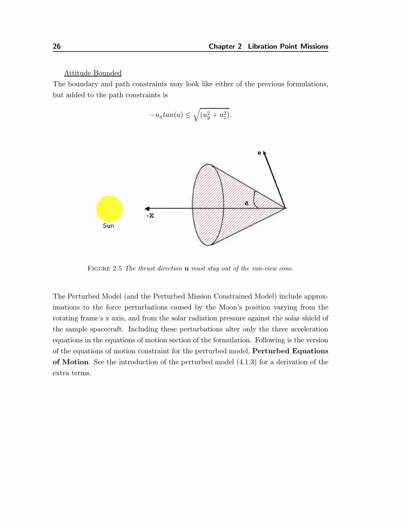
Attitude Bounded
The boundary and path constraints may look like either of the previous formulations,
but added to the path constraints is
−uxtan(a) ≤√
(u2y + u2
z).
Figure 2.5 The thrust direction u must stay out of the sun-view cone.
The Perturbed Model (and the Perturbed Mission Constrained Model) include approx-
imations to the force perturbations caused by the Moon’s position varying from the
rotating frame’s x axis, and from the solar radiation pressure against the solar shield of
the sample spacecraft. Including these perturbations alter only the three acceleration
equations in the equations of motion section of the formulation. Following is the version
of the equations of motion constraint for the perturbed model, Perturbed Equations
of Motion. See the introduction of the perturbed model (4.1.3) for a derivation of the
extra terms.

2.4 Mission Design Optimal Control Problem 27
Perturbed Equations of Motion
x(t) − vx(t) = 0
y(t) − vy(t) = 0
z(t) − vz(t) = 0
vx(t) − 2vy(t) − x(t) +(1 − µ)(x(t) − µ)
r13(t)3
+µ(x(t) + 1 − µ)
r23(t)3−
ux(t)
m(t)−
gmoon cos(α(t))
m
−.9 SRP (surface area) cos(angle between shield normal and − x vector)
(distance from 1 AU)2 (m(t))= 0
vy(t) + 2vx(t) − y(t) +(1 − µ)y(t)
r13(t)3+
µy(t)
r23(t)3−
uy(t)
m(t)−
gmoon sin(α(t))
m(t)= 0
vz(t) +(1 − µ)z(t)
r13(t)3+
µz(t)
r23(t)3−
uz(t)
m(t)= 0
m(t) +‖u(t)‖1
Isp ∗ g= 0,
for all t : [t0, tf ].
The secondary mission example (Chapter 5) uses the original force model, but has
two spacecraft, and therefore some extra constraints. The cost function is still the
sum of all the control variables, but these now include those for both spacecraft, so it
represents the sum of fuel use for all spacecraft in the formation. There are twice as
many variables because the states and controls are repeated for the second spacecraft.
This means that the equations of motion are doubled; there is a repetition with the
first set applying to spacecraft one and the second set applying to spacecraft two. Note,
however, that for ease of comparison with previous work, the mass is not a state variable,
so the controls are the pure accelerations at each time rather than the thrust force. The
final distance constraint is only defined for one spacecraft since the formation distance
constraint would cause other spacecraft to also end their path in the L2 vicinity. The
added constraints are the distance between the two spacecraft and the requirement that
the two spacecraft have similar fuel use. The examples here all use initial position
bounds. Some of the examples further include a periodic constraint. The formulation
for the formation examples follows.
Find the state vector s(t) with elements
s = [x1(t), y1(t), z1(t), vx1(t), vy1(t), vz1(t), x2(t), y2(t), z2(t), vx2(t), vy2(t), vz2(t)]

28 Chapter 2 Libration Point Missions
with subscript 1 and 2 for spacecraft 1 and 2, and u(t), the control vector with elements
u = [ux1(t), uy1(t), uz1(t), ux2(t), uy2(t), uz2(t)],
which minimize the cost
J =Ns∑
i=1
Ji =
∫ tf
t0
Ns∑
i=1
∥
∥ui(t)∥
∥
1dt,
where Ns = 2. This is subject to
x1(t) − vx1(t) = 0
y1(t) − vy1(t) = 0
z1(t) − vz1(t) = 0
vx1(t) − 2vy1(t) − x1(t) +(1 − µ)(x1(t) − µ)
r1s1(t)3+
µ(x1(t) + 1 − µ)
r2s1(t)3
−ux1(t) = 0
vy1(t) + 2vx1(t) − y1(t) +(1 − µ)y1(t)
r1s1(t)3+
µy1(t)
r2s1(t)3− uy1(t) = 0
vz1(t) +(1 − µ)z1(t)
r1s1(t)3+
µz1(t)
r2s1(t)3− uz1(t) = 0
x2(t) − vx2(t) = 0
y2(t) − vy2(t) = 0
z2(t) − vz2(t) = 0
vx2(t) − 2vy2(t) − x2(t) +(1 − µ)(x2(t) − µ)
r1s2(t)3+
µ(x2(t) + 1 − µ)
r2s2(t)3
−ux2(t) = 0
vy2(t) + 2vx2(t) − y2(t) +(1 − µ)y2(t)
r1s2(t)3+
µy2(t)
r2s2(t)3− uy2(t) = 0
vz2(t) +(1 − µ)z2(t)
r1s2(t)3+
µz2(t)
r2s2(t)3− uz2(t) = 0
for all t : [t0, tf ], where risk = distance from body i to spacecraft k; the boundary
conditions,
(x1(tf ) − (1 − µ − r2−L2))2 + y1(tf )2 + z1(tf )2 ≤ (αL)2
J1 = J2,
where 0 ≤ α ≤ 1 and L is the distance between the Earth/Moon and L2; and the path
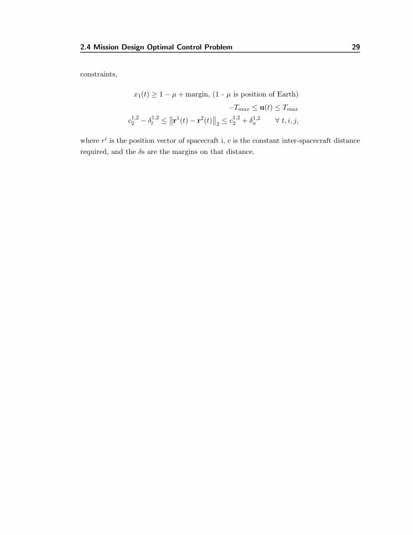
2.4 Mission Design Optimal Control Problem 29
constraints,
x1(t) ≥ 1 − µ + margin, (1 - µ is position of Earth)
−Tmax ≤ u(t) ≤ Tmax
c1,22 − δ1,2
l ≤∥
∥r1(t) − r2(t)∥
∥
2≤ c1,2
2 + δ1,2u ∀ t, i, j,
where ri is the position vector of spacecraft i, c is the constant inter-spacecraft distance
required, and the δs are the margins on that distance.

30

Chapter 3
Solving the
Optimal Control
Problem
All but the simplest optimal control problem must be solved numerically. There are
two basic approaches often termed direct and indirect. An indirect method utilizes the
first-order conditions for optimality given by the Pontryagin’s maximum principle[7].
To solve for the solution of these conditions requires solving a two point boundary value
problem whose dimension is two times the number of state variables. It is simpler
and easier computationally to discretize the optimal control problem (a direct method).
However, the direct approach may not satisfy the optimality conditions in the limit.
While the discretization will not be driven to the limit, it is important to consider the
property of the limit because we would like to be able to state the error between the
solution found and the true solution. This error is related to the size of the discretiza-
tion. We can show that the solution obtained does satisfy this property for many of
the optimality conditions and in particular the feasibility conditions. This is clearly
important for the solution to be tenable. It then follows if we have not satisfied the
full optimality conditions (although we often do) it may mean there is a better feasible
control than the one we have found. How important it is to find a better control in
that case depends on the size of that error from the true optimal solution relative to
the errors that can be expected in the hardware implementation of the controls and
navigation measurements. The acceptable error also depends on the stage of the design
process for which the problem is being solved.
The resulting discrete problem is a nonlinear finite-dimensional optimization prob-
lem and may be solved numerically by standard algorithms for this problem. Inevitably
the discretization process leads to large nonlinear programs. The optimization algo-
rithm used here is a sequential quadratic programming (SQP) method, implemented in
the software SNOPT (produced by the Stanford Systems Optimization Lab, see section
3.2.2 for details), which is explicitly designed to solve large problems.
31

32 Chapter 3 Solving the Optimal Control Problem
There are a plethora of ways to discretize the optimal control problem[30]. The
method of discretization leads to both different theoretical and numerical properties
and to different sizes of discrete problem to obtain the same degree of approximation.
The difference in size may be substantial. The discretization methods compared in
the following section all use SNOPT to ensure it is only the discretization process that
differs.
3.1 Discretization of the Optimal Control Problem
***diagram In this section, a general overview of discretization methods is given,
followed by three in-depth discussions of particular methods. These were the methods
explored for discretizing the optimal control problem presented in this thesis: user calcu-
lated divisions and finite differencing (3.1.1), direct collocation (3.1.2), and pseudospec-
tral (3.1.3). The pseudospectral method was eventually chosen over a direct collocation
method because of the need to look at optimality when using a new approach to an
optimal control problem.
Shooting methods are a common way to discretize an optimal control problem.
Shooting methods approximate the state equations by integrating the vector field. The
time period may be divided into intervals. The state variables at the ‘knots’ between
each interval are the variables for the discretized problem. The differential equations
describing the dynamics of the system (called state equations because they define the
relationship of the state derivatives to the state variables) are solved over each inter-
val by numerical intergration; typically Euler or Runge Kutta. An explicit integration
identifies the discretization as multiple shooting because it integrates over multiple time
arcs, while an implicit integration is used in the collocation method. With the implicit
integration, the state and controls are optimization variables at each point of the in-
tegration as well as at the knots. So if using an n-degree Runge Kutta formula, the
collocation formulation has n times more variables than the multiple shooting formula-
tion of the same problem which only puts optimization variables at the knots between
shooting arcs. This does not make the collocation formulation a longer problem to solve
however, and may make it faster because the first derivatives are easier to compute. Col-
location is less accurate in terms of the state equations though because of the implicit
integration. Direct collocation does not converge to the solution of the optimal con-
trol problem because an Nth-order integration scheme for the differential equations may
not necessarily lead to an Nth-order approximation scheme for the dual variables[35].
The constraints Jacobian and objective function Hessian are sparse for both multiple
shooting and collocation. There is also a single shooting method in which the control

3.1 Discretization of the Optimal Control Problem 33
vector represents coefficients in a polynomial that approximates the control function.
This function encompasses the state equations, eliminating the state variables. The
components of the control vector are the variables, and the objective and constraint
functions are formulated in terms of this vector. This creates a smaller but more dense
problem. In the single shooting formulation, the objective function is very sensitive to
the control variables, so it can require a larger number of timesteps, i.e. a finer grid, to
be stable. A more detailed description of all these methods can be found in Ref.[31].
Another type of discretization approximates not just the states, but also the con-
trols, and sometimes state derivatives as polynomials and interpolates to define the
discrete states and controls. These methods can be called differentiation-based rather
than integration-based[30]. The Hermite-Simpson method uses a Hermite interpolating
polynomial over each interval based on the states and state derivatives at the end points.
There is an equality constraint applied to the center of each interval that forces the val-
ues of the polynomial and its derivative to match the state equations, which express the
relationship of the continuous state function to the continuous state derivatives. Pseu-
dospectral methods use Lagrange interpolating polynomials to approximate the states.
The expansion points where the discrete variables are defined are chosen as specific set
of points. One example is the Legendre-Gauss-Lobatto (LGL) points used in the LGL
pseudospectral method. This is the method of choice for the optimal control problem
explored in this thesis, and is explained in more detail in Section 3.1.3.
3.1.1 Experiments with finite differencing and user differentiation
This formulation discretizes the equations of motion, including the impulsive ∆Vs,
into constraints; a set for each time step. This creates a large complicated problem, but
allows the algorithm to proceed even if the current trajectory is physically infeasible as
well as mission-wise infeasible (diverges from L2). Of course an optimal solution is by
definition also a feasible solution, so the final trajectory will still follow the equations
of motion (in their discretized form).
In this first formulation, the optimization problem formulation discretizes the ordi-
nary differential equations of motion using a simple finite difference scheme[33]:
u(t + h) − u(t)
h= u(t) + O(h),
where h = length of time step. The traditional state vector is the position and veloc-
ity at the current time step: X = (x, y, z, x, y, z). The state vector for the optimization
problem is the whole trajectory. Thus the state vector or trajectory for the current
iteration in the optimization program is Z = (X1,X2, .,XN ) , where N is the number of

34 Chapter 3 Solving the Optimal Control Problem
timesteps. For the problem formulations done in this preliminary research, both h and
N are determined by the Matlab differential equation solver when the program calls for
the initial trajectory.
The discretization into time steps then results in three linear equations(e.g. X1 =
X4) and three nonlinear equations (e.g. X4 = f(X1−6) for each time step. The nonlinear
equations, although complicated as they depend on distances from the masses, are
analytically differentiable. This means that the gradient of the nonlinear constraints can
be calculated before the equations are discretized into finite differences. The nonlinear
equations use finite differences to approximate the accelerations, or first derivatives of
X4−6. The linear equations use finite differences to approximate the velocities, or first
derivatives of X1−3.
It is quite valid to pose this as a finite optimization problem by having a certain
number of timesteps, which requires that the maneuvers that add δv are modeled as
impulses. This is because the dynamics and thus period of the orbit about a libration
point are on a very large scale; in fact a scale proportional to the half period of the
Sun-Earth frame rotation. Therefore, the period will be about six months, whereas the
actual burn duration should not be more than a day, and is probably much less.
With an appropriate discretization formulation, SNOPTs feature of elastic nonlinear
constraints is very helpful, and possibly essential, in finding a solution to this simplified
model, and to more highly constrained models.
3.1.2 Direct Collocation Method
The simple model optimization problem was also solved by the package, GESOP[34],
which uses a direct collocation discretization, and SNOPT to solve the discretized prob-
lem. However, the exploration of this method for solving the problem is presented in
this section.
The examples here use the collocation code TROPIC (TRajectory OPtimization us-
ing dIrect Collocation), which was developed by DLR, Junsch(1990), Schnepper(1992).
It is similar to that used in NASA’s OTIS optimization software (which also uses
SNOPT), but has automatic function and parameter scaling. TROPIC approximates
the controls and states over time by third-order Hermite polynomial functions.
Inputs to GESOP include a guess of states and controls at the starting time, and
of the final time, along with bounds. For this problem, the bounds on states are very
wide, the bounds on the controls are the same as the original problem (zero lower bound
and maximum thrust magnitude upper bound), the final time is set to a fixed value.
GESOP then generates an initial guess using the equations of motion and timesteps
as defined by the user. The integrator is a Runge-Kutta-Fehlberg integrator of fifth

3.1 Discretization of the Optimal Control Problem 35
order, using Dormand and Prince formulae. There is a minimum step value to avoid
the integrator getting stuck if the control estimate is not smooth. A discretization
grid, defined by the user set the collocation nodes. To compare the main discretization
method to traditional collocation, the nodes in GESOP are always chosen to be equally
spaced in the examples shown here.
TROPIC applies a scaling transformation as follows. Given original function F , the
scaled function F = DF , where D is a positive constant. The scaling factors, D, are
computed to keep the scaled collocation constraints at each node matching the scales
states. For x(i) at an interval beginning and x(i + 1) at an interval end (between
collocation nodes), the scaled states are
y(i) = d(i) x(i) + c(i) and y(i + 1) = d(i + 1) x(i + 1) + c(i + 1).
The scaling factors in this interval are then
D = (d(i) + d(i + 1))/2.
If the state outside the interval is not optimized, only d(i) or d(i + 1) is used.
Although this scaling is applied, GESOP could not find a feasible solution for the
libration point mission design problem until the state scaling scheme used with the
pseudospectral method (see Section 3.2.3) was additionally applied. For all GESOP
runs, the final distance constraint was half the distance from L2 to Earth. It was
observed that GESOP needs a fairly good input to find an optimal solution with a cost
approximately zero (the cost of the known global optimal). Using the initial state of the
large halo input, which is a feasible position but zero velocity values, the initial guess
propagated by GESOP does not make an orbit shape, but breaks the final distance
constraint fairly early. GESOP was unable to find a feasible solution with this input for
any time period longer than when the distance constraint was broken.
Given the initial state of the sitting at L2 input, which is all zero for position and
velocity, the initial guess propagated again immediately leaves the L2 vicinity, but at
a slightly slower rate. For a time period of 5 TU (0.8 years), GESOP finds an optimal
solution that starts away from L2 and forms a curve about the point. However, this
solution also uses thrust more than half of the time period, so the cost is relatively
large (1.4 DU/TU or 42 km/s). GESOP did not find one of the global optimals for
this starting point. This guess of sitting at L2 yields widely varying results. When the
time was increase to 5.5 TU (0.9 years), GESOP does find a (nearly) zero cost solution
that has a halo orbit shape. With times of 6 and 7 TU, GESOP cannot get feasible,

36 Chapter 3 Solving the Optimal Control Problem
but when the optimal solution with 5.5 TU is loaded at the start of the optimization,
the same optimal orbit is found with an exactly zero cost. With a good starting point,
propagated from the initial state of the full halo input, GESOP can find a global optimal
usually very close to the input, as long as the time period is not too long (less than
about 7 TU). With time periods of 7 to 9 TU (1.1-1.4 years), global optimal solutions
are found, but often as a smaller or larger halo-type or bean-shaped orbit. At 9 TU,
with 35 nodes a local optimal is found with a similar orbit as the propagated input, but
using bang-bang controls, such that the cost is 4.6. However, when this was changed
to 10 nodes in the optimization, leaving 35 steps for simulations (propagation of initial
state), a global optimal was found.
With larger time periods, the solutions for various numbers of nodes mostly are in-
feasible, and rarely are non-zero cost optimals. With the timelength of 4π TU (2 years),
GESOP found an optimal for 15 nodes with 45 nodes for simulation. This solution had
a cost of 0.1 because it had a positive z thrust over the first two nodes. It is likely that
more nodes could help to enable GESOP to see the problem as feasible more often and
so more likely to find a global optimal solution, but after about 50 nodes, there is not
enough space to compute the problem, and up to 50 nodes, it was still unable to see the
problem as feasible.
Starting with a nonzero controls guess for just the positive x control, GESOP is able
to find an optimal solution quite close to the same input with a totally zero controls
guess. With other nonzero guess controls, though, it cannot find an optimal, and is
unable to compute a good enough search direction to get beyond the first iteration of
the algorithm.
For starting points that did not propagate to ‘good’ guesses, but started reasonably
near the L2 point, nearly zero cost optimal solutions were found for some cases with
final times of 4 TU or less. For longer times, the problem was infeasible.
Using a direct collocation method limited the scope of formulations that could be
solved for the optimal design and control of a libration point mission. This method was
sometimes fast for very good input trajectories and relatively short mission simulations,
but it either broke down computationally or had no feasible point when discretizing
simulations longer than about 8 TU or 1.3 years. Some input trajectories that were
infeasible due to their final distance worked to find an optimal solution if the time
period was short and the starting state variables close to that of a halo orbit, but

3.1 Discretization of the Optimal Control Problem 37
in general the set of inputs that work with this discretization method is limited and
forces optimal trajectories to be halo-type orbits of the size suggested by the input.
These results reflect the need for more knots when using third-order polynomials (as
opposed to much larger orders using the pseduospectral method below) to represent the
equations of motion accurately enough to match the discretized constraints. However,
the number of knots needed is limited by memory availability, and was about 50 for
this amount of variables (as described above). When compared to the PS method,
direct collocation is harder to use and leaves less negotiation for minimum-fuel mission
designs when including further constraints and force perturbations. It doesn’t allow
for the wide variety of input trajectories that is seen using the PS method, although it
produces results a little faster with a good input (for this mission design problem).
Table 3.1
Limitations of direct collocation method
Speed Fast for good input, stalled for poor input, or long sim. times
Input Variety No feasible or optimal solution without near-optimal input
Output Variety Only found halo-shaped optimals, when solution possible
No. Timesteps Need larger number to capture dynamics, out of memory for≥50
Sim. Time Limited to a max. of 9 TU for very good input
3.1.3 Pseudospectral Method
The main advantage of pseudospectral discretization is that it chooses the optimal
node placement in time to discretely represent the variables over time used in the op-
timization problem. The nodes are placed at the roots of the Legendre polynomial
(called the Legendre-Gauss-Lobatto (LGL) quadrature nodes), taking advantage of the
theory of Gaussian quadrature, which states that the optimal abscissas of the Gaussian
quadrature formulas are exactly the roots of the orthogonal polynomial over the same
interval and weighting function. Legendre-Gauss quadrature is limited to the interval
[−1, 1] and the weighting function W (x) = 1. The roots of the Legendre polynomials
occur symmetrically about 0. That the Legendre polynomials are orthogonal is to say
that the following relationship holds:
∫ 1
−1Pm(t)Pn(t)dx = δmn
2
2n + 1,

38 Chapter 3 Solving the Optimal Control Problem
where Pm and Pn are the polynomials and δmn is the Kronecker delta, which is 0 when
m 6= n and 1 when m = n. So we can also say of Legendre polynomials that
∫ 1
−1[Pn(t)]2dx =
2
2n + 1.
This method succeeded where the previous methods failed in solving the problem
discussed here without a good estimate of an optimal solution as a guess. It was im-
plented with DIDO[15], a Matlab application package which discretizes an optimization
problem from its continuous form and then calls SNOPT by way of Tomlab wrappers
that provide an interface between Matlab and SNOPT. DIDO does a pseudospectral
discretization[35] of the optimal control problem into a large nonlinear programming
(NLP) problem which is a representation of the continuous (and thus infinite) optimal
control problem as a finite-dimensional optimization problem.
In DIDO, the state and control functions are approximated by Nth degree poly-
nomials; N+1 being the number of nodes. The discrete derivatives of the states and
controls are the derivatives of these functions at each node. They are calculated by the
differentiation matrix D, which itself is calculated using the Nth degree Legendre poly-
nomial and is a function only of the number of nodes (so it is a constant). The original
continuous problem ((2.9)-(2.12)) is translated to the discrete model, which poses the
problem of finding the (N + 1)(Ns + Nu) vector X = s,u that minimizes
J(X) =tf − t0
2
N∑
k=0
F (sk, uk)wk,
where wk are the LGL weights, a function of N and the Nth degree Legendre polynomial,
and subject to the constraints
equations of motiontf−t0
2 f(sk, uk) −∑N
l=0 Dklxl = 0
boundary constraints b(s0, sN ) = 0
path constraints h(sk, uk) ≤ 0
for k=0,...,N. See the continuous problem for function definitions used in this work.
The D matrix is a (N + 1)2 × (N + 1)2 matrix with a block diagonal form, made up of

3.1 Discretization of the Optimal Control Problem 39
submatrix (N + 1) × (N + 1) blocks Dkl =
LN (tk)LN (tl)
1tk−tl
k 6= l
−N(N+1)4 k = l = 0
N(N+1)4 k = l = N
0 otherwise.
For example,
Table 3.2
Submatrix diagonal in D matrix for N = 4
-5.0 6.8 -2.7 1.4 -0.5-1.2 0 1.7 -0.8 0.30.4 -1.3 0 1.3 -0.4-0.3 0.8 -1.7 0 1.20.5 -1.4 2.7 -6.8 5.0 .
These submatrices are each rank deficient by one. The optimization algorithm can
deal with this however because in choosing N independent columns from the Lagrangian
function, it can take some from the Jacobian of the constraints as well as this differen-
tiation matrix.
The state and control vectors, which were functions of time in the continuous model,
consist of N discrete values in this model; evaluating the value of the function at the time
represented by each of the N nodes during each iteration of the optimization algorithm.
It is important to note that the discretized input trajectory is already different than
exactly what is calculated (as described in the Optimization Formulation section) as a
good input because of the choice of nodes. The optimization algorithm starts with the
input trajectory, composed of state and control variables at N nodes. These variables
are the values calculated by estimating state and control functions based on the states
and controls at given times, and then evaluating these functions at the LGL nodes.
The number of nodes chosen for DIDO to use to solve an optimal control problem is
based on the complexity of the problem and length of time simulated. For the libration
point mission design problem, a relatively large number of nodes are needed to capture
the dynamics of the unstable region (although the PS method generally requires many
fewer timesteps than other discretization methods). The large number of variables at
each time as well as the complexity itself motivate limiting the number of nodes in order
to limit the computation time to a reasonable length. The process is much faster if the

40 Chapter 3 Solving the Optimal Control Problem
input is the output from a previous run of DIDO, so a common practice in this work
was to run DIDO with a small number of nodes - about 5-10 nodes per rotation of the
Earth-Sun system or 2π TU. This first run was often (but not always) too rough of a
grid to capture the dynamics and resulted in SNOPT being unable to find a feasible
solution. This was then the input for a second run of the desired number of nodes - 20
to 80 nodes per system rotation, depending on the accuracy desired. The lower end is
enough to produce a clear optimal solution, and the upper end will produce the same
trajectory as a Runga-Kutta integration of the equations of motion with the optimal
control history for at least 2π TU.
3.2 Solution of the Discretized Problem.
The discretized nonlinear programming problem is solved with a sequential quadratic
programming (SQP) algortithm. The problem from the perspective of the optimization
algorithm is formulated here, and the advantages of the implementation of the SQP for
this particular problem are discussed.
3.2.1 Nonlinear Programming Problem
The optimization algorithm does not distinguish the nonlinear programming prob-
lem solved here as an optimal control problem. The variables consist of every state
and control at every node (in time). These all make up the variable vector, X. The
nonlinear programming problem is
find X that minimizes J(X)
subject to BL ≤ (X,C(X), AX) ≤ BU ,
where BL and BU are lower and upper bounds, J must be smooth and scalar, C(X) is
a vector of smooth nonlinear constraint functions, and A is a sparse matrix such that
AX are any linear constraints. The first and second derivatives of J and C are used in
the optimization algorithm.
3.2.2 Algorithm Details
An SQP algorithm was implemented using the software SNOPT[16], licensed by the
Systems Optimization Laboratory at Stanford University[32]. The algorithm routines
in SNOPT are designed to handle large-scale problems, and take advantage of the
sparsity in the matrices of the discretized problem that result from a small number

3.2 Solution of the Discretized Problem. 41
of degrees of freedom. These qualities make SNOPT an efficient solver for trajectory
design in a complex dynamical space. The degrees of freedom are limited by restriction
that the trajectory satisfy some equations of motion, while the complexity requires
representation at more points in time to adequately capture the dynamics. The amount
of time points used results in thousands of variables and thousands of constraints in
the discretized problem for which SNOPT is well-suited. The approach of exploring
the design space by allowing any kind of input trajectory and control rather than a
near-optimal reference orbit is also made possible by a characteristic of SNOPT. If
the current QP subproblem is infeasible, it enters an ‘elastic’ mode which minimizes
constraint violations while allowing the main optimization algorithm to continue into a
feasible area. The optimization algorithm is complete when it finds a minimum in the
cost function within a set optimization tolerance, that meets the constraint function
within a set feasibility tolerance.
3.2.3 Implementation Analysis
Calling SNOPT from DIDO, the derivatives of functions are not defined, so the first
derivatives are estimated with finite differences[33] by SNOPT. The approximation of
the second derivatives in the form needed at each iteration is part of the algorithm, in
its Hessian approximation.
SNOPT succeeds well in solving the discretized problem even with hundreds of nodes
(this is also due to the form resulting from the PS discretization) despite the lack of
accurate derivatives. It also takes a very reasonable amount of time (on the order of
a few minutes for the largest formulations), but only if the variables are appropriately
scaled. This means that the variables are multiplied by a factor (possibly a different
number for each state and control) before being input into the optimization algorithm.
The factor is usually one that puts their maximum value between 0.1 and 1, but in
some cases, the factor needed to be one or two magnitudes larger. Without scaling the
problems either took days to solve or could not find a feasible point.

42

Chapter 4
Results for an
Example Mission
In this and the next chapter we report the results from testing the algorithms de-
scribed on the problem of libration point mission design; the optimal control problem.
The testing has several purposes. We first demonstrate that the Pseudospectral Method
performs considerably better than the alternative methods of discretization. Only sim-
ple models were needed to reach these conclusions since the alternatives to the PS
method performed poorly even on the simplest problem. Another purpose is to show
that the mission design problem is in fact solvable without breaking it into several steps
and making assumptions about the orbit, and it is in fact solvable for an optimal point
without starting from a ”good guess”.
Although the approach we adopt can be applied to any libration point with similar
results, we choose to design and control formations about the Sun-Earth L2 point be-
cause of the complicated constraints on some of the missions currently proposed at this
location; thus, we have,
µ = 2.448 × 10⁻⁶
rL = (1 − µ + 0.01, 0, 0) DU
in the barycentric frame, where DU is the distance unit equal to the astronomical
unit, AU . The origin in these examples is shifted to L2 to improve variable scaling, so
rL = (0, 0, 0).
This chapter is divided into results of posing the simple problem: keep a spacecraft
in the libration point area for a given time period, and the results of posing the more
complex problem of adding the types of mission constraints that will be imposed on
large telescope spacecraft. This approach allows those more complicated constraints
to be considered during the initial design stage, which will allow a better final design.
The next chapter contains the result of applying this approach to create a formation of
several spacecraft in the Sun-Earth L2 vicinity.
43

44 Chapter 4 Results for an Example Mission
4.1 Mission-Unconstrained Results
The following section describes the details of the inputs and constraints along with
the results for cases in which mission constraints are not applied. The only constraints,
aside from the equations of motion, are those which define the basic problem of a
spacecraft with a set starting mass that is free to thrust in any direction at any (discrete)
time with any magnitude within a set maximum in order to be within a certain radius
of the Sun-Earth L2 point at a set ending time. The position of the spacecraft at times
other than the final time is also bound in a few examples.
Mission constraints would be, for example, a requirement about when or in which
direction the engine could produce thrust, a minimum or maximum distance from the
Sun-Earth line, or a periodicity requirement. The result of applying a mission constraint
within this framework will be seen in the next section.
4.1.1 Simple Model Definition
The simple model uses the equations of motion for the circular restricted three-body
problem, without any perturbations, which was described in Section 2.1. As expected
for this model, optimal trajectories are found for zero cost which remain in ‘orbit’ about
L2.
4.1.2 Simple Model Solutions
For each of the following examples, the number of nodes to be used and the value
of the final distance constraint, df are chosen. The other constraints remain the same,
and their form can be seen in the previous section. In addition, an estimate of the
solution is defined as a starting point for the optimization algorithm. The discretization
and optimization software are run with this information, and output the states and
controls at each node that are determined to be an optimal solution (resulting in a local
minimum in the cost function). The estimate of the solution is also in the form of state
variables and control variables, but are given at any list of timesteps, along with the
value of these timesteps. We call this information the ‘input trajectory’.
The input trajectories for these examples are chosen to find different but similar optimal
solutions, and to illustrate the ability of this method to find optimal solutions with
different quality starting points. The input trajectories are halo-shaped orbits, with
variations in velocity information, distance constraint values, and orbit size. There is
also an input of just a few timesteps, all at the L2 point, as a low-quality estimate
example.

4.1 Mission-Unconstrained Results 45
Example 1
As expected for the circular restricted three-body problem, an optimal trajectory is
found for zero cost which remains in ‘orbit’ about L2. In all examples here, we consider
a fixed-horizon problem, and set tf = 4π timeunits(TU) (730 days). The time unit is
equal to the period of the rotation system, which is the inverse of the frequency, 2π radi-
ans per year. The thrust acceleration magnitude constraint is, umax = 0.001 DU/TU2,
where TU , the time unit is 1/(2π) of the period of the of the primary system; i.e. a
year for the Sun-Earth system. The maximum final distance df is .002 DU, 1/5 the
distance between the Earth and L2 (call this distance L). The input states and controls
(the starting point for the optimization algorithm) are the position coordinates of a halo
orbit. The velocities and controls are zero, and the mass stays at the initial normalized
mass of 1. This means the initial estimate of the solution is infeasible since the equations
of motion do not hold. The input trajectory is produced with the equations,
x = −Ax ∗ cos(2 ∗ t)
y = Ay ∗ sin(2 ∗ t)
z = Az ∗ sin(2 ∗ t + pi/4)
for t = 0; .01; .02...4π,
where
Ax = 206, 000 km,Ay = 665, 000 km,Az = 110, 000 km.
The initial state of the input for this example is (in DU and DU/TU):
x(t0) = −1.377 × 10⁻³, vx(t0) = 0
y(t0) = 0, vy(t0) = 0
z(t0) = 0.520 × 10⁻³, vz(t0) = 0.
To reduce the computation time, the initial state of the solution was bound to a
box of 0.01 DU on either side of the about input initial state. In another technique to
reduce computation time, the problem was first solved for 40 nodes, and the solution
used as input to solve the problem with 200 nodes, which produced a clear solution.
This solution was then used as an input to compute a 400 node solution in order to
achieve the accuracy needed to make the comparison shown in Fig. 4.4.

46 Chapter 4 Results for an Example Mission
As noted earlier, we used DIDO[15] with SNOPT[16] to solve the optimization prob-
lem. A solution to the problem for a choice of 400 nodes (roughly, a 399th-order Legendre
polynomial) is shown in Fig. 4.1. This solution is clearly globally optimal because it has
zero cost, i.e. J = 0 ⇔ u = 0. The optimal controls are almost all zero at each node as
shown in Fig. 4.2.
Figure 4.1 Simple Model Example 1: An Optimal Trajectory for Large Halo Input
Note that there is just one non-zero control variable, at the first node, and it is
about 1 × 10⁻⁸ DU/TU2, compared to the maximum allowed magnitude of 1 × 10⁻³.
This may be considered noise since it is smaller than the tolerances and the trajectory
would be the same within these tolerances if this variable were exactly zero. So the cost

4.1 Mission-Unconstrained Results 47
0 2 4 6 8 10 12−1
−0.5
0
0.5
1x 10
−7
TU
Nor
mal
ized
Thr
ust
Control Vector FunctionsUx at nodesUx functionUy at nodesUy functionUz at nodesUz function
Figure 4.2 Simple Model Example 1: Thrust over time
can be considered zero.
The claim of optimality is based on several tests[15]. One of these tests is the
approximate constancy of the Hamiltonian with an average value equal to zero.[13] The
Hamiltonian was defined in Chapter 2 (Equation 2.13). For illustration of this test, the
non-zero values of the Hamiltonian for this example are shown to be trivially small in
Fig. 4.3. In order to practically demonstrate the convergence of the solution, we use the
optimal initial conditions (in DU and DU/TU),
x(t0) = 0.24 × 10⁻⁴, vx(t0) = 5.27 × 10⁻⁴
y(t0) = −6.75 × 10⁻⁴, vy(t0) = −79.03 × 10⁻⁴
z(t0) = −2.67 × 10⁻⁴, vz(t0) = −9.57 × 10⁻⁴
to propagate the solutions using ode45 in Matlab. Fig. 4.4 shows a comparison of the
optimized velocity states to the propagated velocity states of one of the spacecraft up
to the point of divergence. It is apparent that the propagated states track fairly well
to the optimized ones up to π TU, indicating that it takes 400 nodes over this time
period for a solution accurate enough for preliminary design considerations for one year
in the current formulation. This is because the timestep at which the solution diverges

48 Chapter 4 Results for an Example Mission
0 50 100 150 200 250 300 350 400−7
−6
−5
−4
−3
−2
−1
0
1
2x 10
−7 Hamiltonian
Figure 4.3 Simple Model Example 1: Evolution of the Hamiltonian; note the scale on theordinate
from the propagated trajectory increases proportionally to the number of nodes. For
the rest of the examples the number of nodes will be only large enough to produce a
clear optimal solution, since solutions that more closely align with a differential equation
solver solution can be easily found with an increase in the number of nodes.
Example 2
The input states and controls (the starting point for the optimization algorithm)
are again the position coordinates of a halo orbit with the velocities and controls zero,
but this orbit is only 10% of the size of the previous example’s input. The input mass
is again 1 at all nodes. There is no bound on the initial state, and the maximum final
distance df is L, the distance between the Earth and L2. The input trajectory is pro-
duced with the equations,

4.1 Mission-Unconstrained Results 49
0 0.5 1 1.5 2 2.5 3−0.015
−0.01
−0.005
0
0.005
0.01
0.015
TU
DU
/TU
Optimal vs Propagated Velocities
VXpropVXoptVYpropVYoptVZpropVZopt
Figure 4.4 Simple Model Example 1: Comparison of the velocity states to those propagatedby ODE45 in Matlab (dotted)
x = −Ax ∗ cos(2 ∗ t)
y = Ay ∗ sin(2 ∗ t)
z = Az ∗ sin(2 ∗ t + pi/4),
where
Ax = 20, 600 km,Ay = 66, 500 km,Az = 11, 000 km.
The solution shown here was computed first for 25 nodes for which no feasible solution
could be found, and then iterated for 125 nodes.
The optimal controls are all exactly zero at each node.
Example 3
The input states and controls are the same as the previous example’s input. There is
still no bound on the initial state, but the maximum final distance df has been reduced
to .005 DU, or L/2. The input trajectory is produced with the equations,

50 Chapter 4 Results for an Example Mission
x = −Ax ∗ cos(2 ∗ t)
y = Ay ∗ sin(2 ∗ t)
z = Az ∗ sin(2 ∗ t + pi/4),
where
Ax = 20, 600 km,Ay = 66, 500 km,Az = 11, 000 km
The solution shown here was computed first for 25 nodes for which an optimal but too
coarse solution was found, and then iterated for 125 nodes.

4.1 Mission-Unconstrained Results 51
Figure 4.5 Simple Model Example 2: An Optimal Trajectory for Small Halo Input, df = D
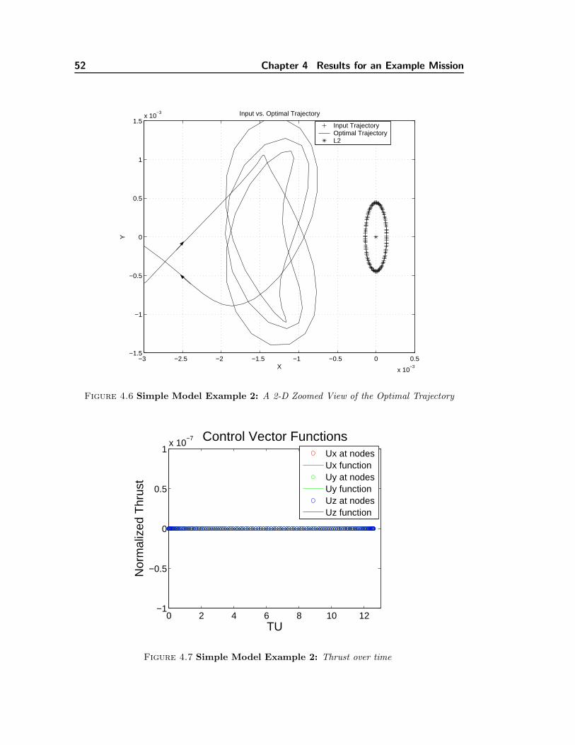
52 Chapter 4 Results for an Example Mission
−3 −2.5 −2 −1.5 −1 −0.5 0 0.5
x 10−3
−1.5
−1
−0.5
0
0.5
1
1.5x 10
−3
X
YInput vs. Optimal Trajectory
Input TrajectoryOptimal TrajectoryL2
Figure 4.6 Simple Model Example 2: A 2-D Zoomed View of the Optimal Trajectory
0 2 4 6 8 10 12−1
−0.5
0
0.5
1x 10
−7
TU
Nor
mal
ized
Thr
ust
Control Vector FunctionsUx at nodesUx functionUy at nodesUy functionUz at nodesUz function
Figure 4.7 Simple Model Example 2: Thrust over time

4.1 Mission-Unconstrained Results 53
Figure 4.8 Simple Model Example 3: An Optimal Trajectory for Small Halo Input, df =D/2

54 Chapter 4 Results for an Example Mission
−3 −2.5 −2 −1.5 −1 −0.5 0 0.5
x 10−3
−1.5
−1
−0.5
0
0.5
1
1.5x 10
−3
X
Y
Input vs. Optimal Trajectory
Input TrajectoryOptimal TrajectoryL2
Figure 4.9 Simple Model Example 3: A 2-D Zoomed View of the Optimal Trajectory
The optimal controls are almost all zero at each node as shown in Fig. 4.10. Note
that two non-zero control variables, at the first and second node, in the z direction at
about 1 × 10⁻⁵ DU/TU2, and then in the x direction at about 5 × 10⁻⁵ DU/TU2,
compared to the maximum allowed magnitude of 1 × 10⁻³. This is larger noise than
the first example, but is still small enough that it is most likely due to amplification
because of placement of nodes, and would disappear with a larger number of nodes.
Example 4
The input states in this example are both positions and velocities of a sample halo
orbit. The orbit is calculated using the same equations of motion that are a constraint in
the optimization problem. The input trajectory calculator varies the starting velocities,
targeting zero velocity in the y direction at the crossing of the x axis. This results in

4.1 Mission-Unconstrained Results 55
0 100 200 300 400 500 600 700−1
−0.8
−0.6
−0.4
−0.2
0
0.2
0.4
0.6
0.8
1x 10
−3 Thrust
Days
XYZnodes
Figure 4.10 Simple Model Example 3: Thrust over time
an approximation of a natural halo orbit, so the input control variables are all zero.
Like the previous examples, the mass component of the input state vector is always at
the ‘full’ value, one instead of zero. There is no bound on the initial state, and the
maximum final distance df is .005 DU, or L/2. This constraint is active as the optimal
trajectory diverges from the almost repeating ‘orbit’ to end at this distance (toward
Earth) on the final node. The resulting input trajectory starts at the same position as
the previous examples, but with a velocity of about 0.0046DU/TU in the y direction.
Figures 4.11 and 4.12 show the optimal solution found with this more complete halo
orbit as a starting point. It was computed first for 25 nodes for which an optimal but
too coarse solution was found. This was the input for a 35 node solution which was
optimal and zero cost but still somewhat course, which was then iterated into a 125
node solution for accuracy and consistency. The optimal controls are all exactly zero at
each node, so the thrust over time plot is not shown.
Example 5
The input states and controls are zero, which means the input trajectory is station-
ary at L2. The mass component of the input state vector is one at all nodes. There
is still no bound on the initial state, and the maximum final distance df is L. But this
constraint is not active because the optimal trajectory starts closer to the Earth and

56 Chapter 4 Results for an Example Mission
orbit L2, ending close to the point; about 1% of the maximum final distance allowed by
the distance constraint. The input trajectory is the following,
x(0) = 0, except m(0) = 1
x(2π) = 0, except m(2π) = 1
x(4π) = 0, except m(4π) = 1.
As seen above, there are only 3 nodes for the input. The solution shown below (Fig.
4.13) was computed first for 35 nodes for which an optimal but too coarse solution was
found, and then iterated for 125 nodes. The optimal controls are all exactly zero at
each node (Fig. 4.14).
Table 4.1
Summary of Results: Simple Model
Ex. Input Trajectory df x(0) Bounds Nodes Optimal Control
1 large halo, x, y, z only L/5 ±L box 400 10−8 at node 12 small halo, x, y, z only L none 125 all 03 small halo, x, y, z only L/2 none 125 10−5 at node 1 & 24 halo with full state L/2 none 125 all 05 3 nodes: stationary at L2 L none 125 all 0
We have seen that increasing the number of nodes increases the accuracy of the
solution. A larger number of nodes also means a longer processing time, so it is advisable
to choose a number just large enough to capture the accuracy for the mission time-length
being used, about 30 to 80 per year. (This informed the choice of 125 nodes in the above
examples.) In order to quantify this performance of the discretization and optimization
algorithms relative to number of nodes, an optimal solution with 25 nodes was chosen
as an input to produce a few optimal solutions of more gradually increasing number
of nodes. The CPU time was measured along with the accuracy, as measured by the
magnitude of violation of the constraints (Fig. 4.15).
Because this experiment is based on a 25 node solution, the error in the optimal
output for 25 nodes is significantly lower that it would be for a non-optimal input, or an
optimal input of fewer nodes. The exponential decrease in error with increasing nodes
can be seen in the remaining data points.

4.1 Mission-Unconstrained Results 57
Figure 4.11 Simple Model Example 4: An Optimal Trajectory for Full Halo Orbit Input,df = D/2

58 Chapter 4 Results for an Example Mission
−1.5
−1
−0.5
0
x 10−3
−6
−4
−2
0
2
4
6
x 10−4
−6
−4
−2
0
2
4
6
x 10−4
X
Y
Z
Input vs. Optimal Trajectory
Input TrajectoryOptimal TrajectoryL2Earth
Figure 4.12 Simple Model Example 4: A Zoomed View of the Optimal Trajectory, df =D/2

4.1 Mission-Unconstrained Results 59
Figure 4.13 Simple Model Example 5: An Optimal Trajectory for Stationary L2 Input,df = D
0 2 4 6 8 10 12−1
−0.5
0
0.5
1x 10
−7
TU
Nor
mal
ized
Thr
ust
Control Vector FunctionsUx at nodesUx functionUy at nodesUy functionUz at nodesUz function
Figure 4.14 Simple Model Example 5: Thrust over time

60 Chapter 4 Results for an Example Mission
Figure 4.15 Speed and Accuracy vs Number of Nodes

4.1 Mission-Unconstrained Results 61
4.1.3 Perturbed Model Definition
In the following examples the equations of motion include the solar radiation pres-
sure and lunar gravity as perturbations on the force model. The solar radiation pressure
is modeled as a force in the positive x direction which varies only with distance. The
perturbation of the moon’s gravity is modeled as a cyclical force within the x-y plane.
It has a mostly negative x direction with a y component that varies over time between
positive and negative. Below are the equations for the acceleration due to each which
are added onto the acceleration equations in the differential equations of motion (e.g
ax = acceleration added to x acceleration equation).
Solar Radiation Pressure
SRP= 4.6 × 10⁻⁶N/m2at 1 AU
surface area = 260 m2
ax =.9 SRP (surface area) cos(angle between shield normal and − x vector)
(distance from 1 AU)2 (mass)
Lunar Gravity
P = period of the moon in rotating frame = 29.4 days
M = maximum angle between x axis and L2-moon line
= arctan(Moon-Earth line / L2-Earth line)
α = M , time=0 at moon x-axis crossing
gmoon = gravitational acceleration of moon at L2 = 6 × 10⁻⁶km/s2
ax =gmoon cos(α)
mass
ay =gmoon sin(α)
mass
4.1.4 Perturbed Model Solutions
All of the following results had a maximum thrust magnitude constraint of 1 and
final distance constraint of L/2. These first set of three examples use as input the states
describing a large halo orbit without velocity information. They vary in the amount of
constraints on the position state variables.

62 Chapter 4 Results for an Example Mission
02
46
8
0
5
10
15
20
−6
−4
−2
0
X
Input and Optimal Trajectory
Y
Z
optimalL2Earthstartend
Figure 4.16 Perturbed Model Example 1: Optimal trajectory with no bounds on states
Example 1
With no bounds on the states, the optimal trajectory found starts far from the libra-
tion point and makes an arc to bring it within the final distance constraint. The longer
the simulation time, the farther away it starts, so the example shown here (Fig. ??) is
for the short time period of π/2 TU or 3 months. This result is different than with the
unperturbed model, where the optimization routine found an optimal closer in size to
the input, staying relatively close to the libration point without any path constraints on
the position to force that characteristic. This trajectory requires a large thrust profile
(Fig. 4.18). This design may be desirable if the trajectory is coming from outside the
Earth/Moon system. If this is not the case, we may use position constraints to eliminate
trajectories such as this.

4.1 Mission-Unconstrained Results 63
−0.01 −0.005 0 0.005 0.01−0.01
−0.008
−0.006
−0.004
−0.002
0
0.002
0.004
0.006
0.008
0.01Input and Optimal Trajectory
X
Y
InputOptimalL2Earth
Figure 4.17 Perturbed Model Example 1: Optimal trajectory with no bounds on states(zoomed)
Example 2
Here, a boundary constraint bounds the positions at the starting time to ±L in each
direction. This results in a starting and final position near the libration point, but the
trajectory is still very large, making a circle that goes beyond the orbital path of Mars
(Fig. 4.19). The control vector part of the solution again requires significant thrust at a
few points, especially along the y axis (Fig 4.20). This also could be a useful trajectory
shape, and could be further constrained to design a Mars cycler, for example. Also, if
closer distance was not as important for a particular astronomical observation mission
as it may be for solar power or data transfer, and this were a lower minimum in the cost
function than other closer trajectories. (We will see though that in exploring the design
space further we find an example of a lower minimum in a smaller orbit.) However,
if it is more important to maintain a smaller communication delay or maximum solar
power, we can use a path constrain to limit the position of the spacecraft at all times.

64 Chapter 4 Results for an Example Mission
0 0.2 0.4 0.6 0.8 1 1.2 1.4 1.6−0.2
−0.15
−0.1
−0.05
0
0.05
0.1
0.15
TU
Nor
mal
ized
Thr
ust
Control Vector Functions
Ux at nodesUx functionUy at nodesUy functionUz at nodesUz function
Figure 4.18 Perturbed Model Example 1: Thrust over time with no bounds on states
Example 3
In this last example in the set, in addition to the initial state bound, the positions at
all times are bound to ±2L. This forces the optimization routine to find a minimum in
the cost function that results in a trajectory of similar size to the input large halo orbit
(Fig. 4.21). Increasing the constraints on the position has increased the amount of fuel
needed. This example has a control vector that reaches maximum magnitude of thrust
along all three axes at different nodes (Fig. 4.22). Also, it must use a curve rather than
small periods of thrust between longer periods of zero thrust (engines off). This would
not be acceptable for a telescope mission since the engines must be off for observations.
Either further constraints on the controls would be needed, or selection of a different
base minimum fuel trajectory found in the design space by varying the input.

4.1 Mission-Unconstrained Results 65
−0.02 0 0.02−0.06
−0.04
−0.02
0
0.02
0.04
0.06
Input and Optimal Trajectory
X
Y
InputOptimalL2Earth
Figure 4.19 Perturbed Model Example 2: Optimal trajectory with initial states bound

66 Chapter 4 Results for an Example Mission
0 1 2 3 4 5 6 7−0.06
−0.04
−0.02
0
0.02
0.04
0.06
TU
Nor
mal
ized
Thr
ust
Control Vector Functions
Ux at nodesUx functionUy at nodesUy functionUz at nodesUz function
Figure 4.20 Perturbed Model Example 2: Thrust over time with initial states bound

4.1 Mission-Unconstrained Results 67
−10−5
0
x 10−3
−4−2
02
46
x 10−3
−5
0
5
x 10−3
X
Input and Optimal Trajectory
Y
ZInputOptimalL2EarthStart point
Figure 4.21 Perturbed Model Example 3: Optimal trajectory with states bound

68 Chapter 4 Results for an Example Mission
0 1 2 3 4 5 6 7−1
−0.5
0
0.5
1
TU
Nor
mal
ized
Thr
ust
Control Vector FunctionsUx at nodesUx functionUy at nodesUy functionUz at nodesUz function
Figure 4.22 Perturbed Model Example 3: Thrust over time with states bound

4.1 Mission-Unconstrained Results 69
The last two examples try some inputs very different from the large halo to find the
illustrate the variety found by simple input changes. The states have the same boundary
and path constraints as the previous example, so the solutions will be limited in size to
±2L about the libration point (Fig. ??). The control vectors of the solution show that
much smaller thrusts are required for these trajectories (Fig. ??). This next example
uses the three points over time at L2 with no velocity as the input, i.e. all zero values
in the state and control vector at three timesteps.
Example 4
−10 −8 −6 −4 −2 0 2
x 10−3
−5
−4
−3
−2
−1
0
1
2
3
4
5
x 10−3 Input and Optimal Trajectory
X
Y
10 node result (on L2)OptimalL2EarthStart point
Figure 4.23 Perturbed Model Example 4: Optimal trajectory with states bound

70 Chapter 4 Results for an Example Mission
0 1 2 3 4 5 6 7−10
−8
−6
−4
−2
0
2
4x 10
−4
TU
Nor
mal
ized
Thr
ust
Control Vector Functions
Ux at nodesUx functionUy at nodesUy functionUz at nodesUz function
Figure 4.24 Perturbed Model Example 4: Thrust over time with states bound

4.1 Mission-Unconstrained Results 71
The last example has an input much like the previous except it is sitting at the point
halfway between Earth and L2.
Example 5
−0.01 −0.008 −0.006 −0.004 −0.002 0
−3
−2
−1
0
1
2
3
x 10−3 Input and Optimal Trajectory
X
Y
10 node result (at −.005,0)OptimalL2EarthStart point
Figure 4.25 Perturbed Model Example 5: Optimal trajectory with states bound
The value of the cost function for the solutions found with the stationary point
inputs are much lower minimums than those found with the large halo input, as is
reflected by the smaller magnitudes of thrust in the control vectors. This shows the
value of exploring the design space by using many types of input trajectories, not just
those close to known optimal trajectories for the simplest model.

72 Chapter 4 Results for an Example Mission
0 1 2 3 4 5 6 7−1
−0.8
−0.6
−0.4
−0.2
0
0.2
0.4
0.6
0.8
1x 10
−4
TU
Nor
mal
ized
Thr
ust
Control Vector Functions
Ux at nodesUx functionUy at nodesUy functionUz at nodesUz function
Figure 4.26 Perturbed Model Example 5: Thrust over time with states bound
Table 4.2
Summary of Results: Perturbed Model. tf in TU, Cost in DU/TU and m/s
Ex. Input Trajectory tf State Bounds Nodes Cost Cost
1 large halo, x, y, z only π/2 none 15 0.0035 1042 large halo, x, y, z only 2π initial ±L 25 0.006 1793 large halo, x, y, z only 2π all ±2L 45 0.36 107304 3 nodes: stationary, L2 2π all ±2L 45 8.8 × 10⁻⁶ 0.265 3 nodes: stationary, x = L/2 2π all ±2L 45 6.6 × 10⁻⁶ 0.20

4.2 Mission Constrained Results 73
4.2 Mission Constrained Results
These results are all based on the pertubed model, but also include an added con-
straints on the attitude.
4.2.1 Attitude Constraint Definition
If we assume that the thruster is exactly opposite the center pointing direction of
the sensors and/or telescope, the thrust direction is where the sensors are pointed. (If
the thrust is zero, we assume it will be pointed in some safe direction as non-thrusting
times will be observation times, and observations are all done away from the sun.) So
it is the angle between the thrust direction and the direction toward the sun that has a
minimum allowed value. The thrust direction is the direction of the vector composed of
the total control magnitude along each axis. The direction toward the sun is negative x.
Define ux, uy, uz as the total control magnitudes along each axis, and a is the minimum
sun-sensor angle The constraint looks like a cone about the x axis with half angle a. It
is the negative half of the cone we are concerned with since that is the direction of the
sun. From this cone we see the relationship
Figure 4.27 The thrust direction (defined by the control vector) must stay out of the sun-viewcone.
tan(a) = r/h
If we look at the case where the thrust vector is at the boundary of the cone, we have
h = ux, r =√
u2y + u2
z

74 Chapter 4 Results for an Example Mission
So this boundary can be defined with the equation
tan(a) =
√
u2y + u2
z
ux
We rewrite this equation as
uxtan(a) =√
u2y + u2
z
to avoid dividing by zero.
Since we want to define an inequality constraint that holds when the thrust direction
vector is outside the cone, we want the inequality to be broken when uy and uz are zero
and ux is negative. The inequality must also be true for any positive ux. Since tan(a)
will always be greater than zero (a is the desired minimum sun-spacecraft angle between
zero and 90 degrees), the inequality constraint describing the attitude restriction is
−uxtan(a) ≤√
(u2y + u2
z).
4.2.2 Perturbed Mission Constrained Model Solutions
This first set of examples correspond to the first set in the Perturbed Model section,
but these trajectories include the above constraint, with the maximum angle from the
-x axis set to 40 degrees. The attitude over time for the previous and current section
are then compared for each example. Since the attitude is not an actual variable but
only defined as a constraint of the control vector, it is only valid when the control vector
(thrust acceleration) is non-zero. The attitude plots shown here are calculated based on
the control vector at each node, as the angle from the -x axis. When the control vector
is zero (within tolerance), the attitude is defined as 90 degrees.

4.2 Mission Constrained Results 75
Example 1
−2 −1 0 1 2 30
0.5
1
1.5
2
2.5
3
3.5
4
4.5
Input and Optimal Trajectory
X
Y
InputOptimalL2Earth
Figure 4.28 Constrained Example 1: Optimal trajectory with attitude constraint and statesnot bound

76 Chapter 4 Results for an Example Mission
0 0.2 0.4 0.6 0.8 1 1.2 1.4 1.6−0.04
−0.02
0
0.02
0.04
0.06
0.08
0.1
0.12
TU
Nor
mal
ized
Thr
ust
Control Vector Functions
Ux at nodesUx functionUy at nodesUy functionUz at nodesUz function
Figure 4.29 Constrained Example 1: Thrust over time with attitude constraint and statesnot bound
0 20 40 60 80 1000
20
40
60
80
100
120
140
160
180Attitude
Days
Ang
le fr
om −
x ax
is (
deg)
Figure 4.30 Constrained Example 1: Attitude over time w/out constraint and states notbound

4.2 Mission Constrained Results 77
0 20 40 60 80 100
40
60
80
100
120
140
160
180Attitude
Days
Ang
le fr
om −
x ax
is (
deg)
Figure 4.31 Constrained Example 1: Attitude over time with constraint and states notbound

78 Chapter 4 Results for an Example Mission
Example 2
−0.1 0 0.1 0.2 0.3 0.4 0.5 0.6 0.7
−0.3
−0.2
−0.1
0
0.1
0.2
0.3
Input and Optimal Trajectory
X
Y
InputOptimalL2Earth
Figure 4.32 Constrained Example 2: Optimal trajectory with constraint and initial statesbound

4.2 Mission Constrained Results 79
0 1 2 3 4 5 6 7−0.06
−0.04
−0.02
0
0.02
0.04
0.06
TU
Nor
mal
ized
Thr
ust
Control Vector Functions
Ux at nodesUx functionUy at nodesUy functionUz at nodesUz function
Figure 4.33 Constrained Example 2: Thrust over time with attitude constraint and initialstates bound
0 50 100 150 200 250 300 3500
20
40
60
80
100
120
140
160
180Attitude
Days
Ang
le fr
om −
x ax
is (
deg)
Figure 4.34 Constrained Example 2: Attitude over time w/out constraint but initial statesbound

80 Chapter 4 Results for an Example Mission
0 50 100 150 200 250 300 350
40
60
80
100
120
140
160
180Attitude
Days
Ang
le fr
om −
x ax
is (
deg)
Figure 4.35 Constrained Example 2: Attitude over time with constraint and initial statesbound

4.2 Mission Constrained Results 81
−0.5
0
0.5
1
−0.4−0.2
00.2
0.4
−0.050
0.05
Input and Optimal Trajectory
Original Input45 node result
OptimalL2
EarthStart point
Figure 4.36 Constrained Example 2: Optimal trajectory with constraint and initial statesbound, twice as many nodes
By doubling the number of nodes, the control can take advantage of more points
to apply a small continuous thrust rather than a few larger maneuvers toward the end
of the time period. This reduces the cost by 30%, but this control design would work
better for a low-thrust transfer or station mission than for an observational mission
which needs long periods with the engine off.

82 Chapter 4 Results for an Example Mission
Original Input45 node result
OptimalL2
EarthStart point
Figure 4.37 Constrained Example 2: Optimal trajectory with constraint and initial statesbound, twice as many nodes (zoomed)
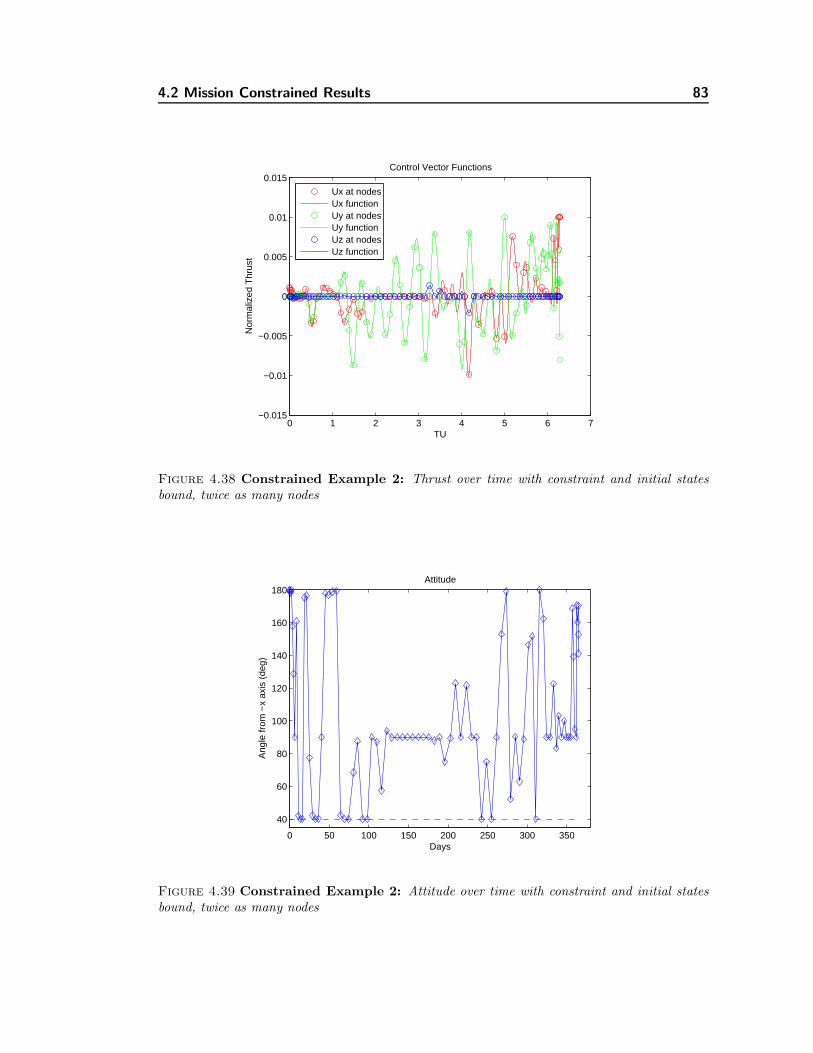
4.2 Mission Constrained Results 83
0 1 2 3 4 5 6 7−0.015
−0.01
−0.005
0
0.005
0.01
0.015
TU
Nor
mal
ized
Thr
ust
Control Vector Functions
Ux at nodesUx functionUy at nodesUy functionUz at nodesUz function
Figure 4.38 Constrained Example 2: Thrust over time with constraint and initial statesbound, twice as many nodes
0 50 100 150 200 250 300 350
40
60
80
100
120
140
160
180Attitude
Days
Ang
le fr
om −
x ax
is (
deg)
Figure 4.39 Constrained Example 2: Attitude over time with constraint and initial statesbound, twice as many nodes

84 Chapter 4 Results for an Example Mission
Example 3
−0.01
0
0.01−0.01
0
0.01
0.02
0.03
0.04
−0.01
0
0.01
Y
Input and Optimal Trajectory
X
Z
InputOptimalL2EarthStart point
Figure 4.40 Constrained Example 3: Optimal trajectory with constraint and states bound

4.2 Mission Constrained Results 85
0 1 2 3 4 5 6 7−1
−0.5
0
0.5
1
TU
Nor
mal
ized
Thr
ust
Control Vector Functions
Ux at nodesUx functionUy at nodesUy functionUz at nodesUz function
Figure 4.41 Constrained Example 3: Thrust over time with constraint and states bound
0 1 2 3 4 5 6 70
20
40
60
80
100
120
140
160
180Attitude
TU
Ang
le fr
om −
x ax
is (
deg)
Figure 4.42 Constrained Example 3: Attitude over time w/out constraint but states bound

86 Chapter 4 Results for an Example Mission
0 1 2 3 4 5 6 70
20
40
60
80
100
120
140
160
180Attitude
TU
Ang
le fr
om −
x ax
is (
deg)
Figure 4.43 Constrained Example 3: Attitude over time with constraint and states bound

4.2 Mission Constrained Results 87
This example corresponds to Example 4 in the previous section, with the attitude
constraint applied to the input of a stationary location at L2.
Example 4
−0.01
−0.005
0
0.005
0.01
−4−2
02
4
x 10−3
−5
0
5
x 10−3
X
Input and Optimal Trajectory
Y
Z
Input (at L2)OptimalL2EarthStart point
Figure 4.44 Constrained Example 4: Optimal trajectory with constraint and states bound

88 Chapter 4 Results for an Example Mission
0 1 2 3 4 5 6 7−1.5
−1
−0.5
0
0.5
1
1.5x 10
−4
TU
Nor
mal
ized
Thr
ust
Control Vector FunctionsUx at nodesUx functionUy at nodesUy functionUz at nodesUz function
Figure 4.45 Constrained Example 4: Thrust over time with constraint and states bound
0 1 2 3 4 5 6 70
20
40
60
80
100
120
140
160
180Attitude
TU
Ang
le fr
om −
x ax
is (
deg)
Figure 4.46 Constrained Example 4: Attitude over time w/out constraint but states bound

4.2 Mission Constrained Results 89
0 1 2 3 4 5 6 70
20
40
60
80
100
120
140
160
180Attitude
TU
Ang
le fr
om −
x ax
is (
deg)
Figure 4.47 Constrained Example 4: Attitude over time with constraint and states bound

90 Chapter 4 Results for an Example Mission
This example corresponds to Example 5 in the previous section, with the attitude
constraint applied to the input of a stationary location halfway between the Earth and
L2.
Example 5
Figure 4.48 Constrained Example 5: Optimal trajectory with constraint and states bound

4.2 Mission Constrained Results 91
0 1 2 3 4 5 6 7−6
−4
−2
0
2
4
6x 10
−5
TU
Nor
mal
ized
Thr
ust
Control Vector Functions
Ux at nodesUx functionUy at nodesUy functionUz at nodesUz function
Figure 4.49 Constrained Example 5: Thrust over time with constraint and states bound
0 50 100 150 200 250 300 350 4000
20
40
60
80
100
120
140
160
180Attitude
Days
Ang
le fr
om −
x ax
is (
deg)
Figure 4.50 Constrained Example 5: Attitude over time w/out constraint but states bound

92 Chapter 4 Results for an Example Mission
0 50 100 150 200 250 300 350 40020
40
60
80
100
120
140
160
180Attitude
Days
Ang
le fr
om −
x ax
is (
deg)
Figure 4.51 Constrained Example 5: Attitude over time with constraint and states bound

4.3 Comparison with Reference Orbit Approach 93
Table 4.3
Summary of Results: Constrained/Unconstrained Comparison. Cost in DU/TU
Ex. Input Min. angle Min. angle Cost Cost(Unconstr.) (Constr.) (Unconstr.) (Constr.)
1 large halo 1◦ 44◦ 0.0035 0.00372 large halo 0 40 0.006 0.00563 large halo 90 40 0.36 0.484 L2 point 0 40 8.8 × 10⁻⁶ 2.3 × 10⁻⁶
5 x = L/2 0 40 6.6 × 10⁻⁶ 6.1 × 10⁻⁶
4.3 Comparison with Reference Orbit Approach
In order to make some comparison of these results with what is achieved by the
general approach of first choosing a reference orbit and then designing the controls to
match this path, the reference orbit approach is here approximated within the concurrent
approach. An optimal solution from the simple model results is used as an input.
The equation of motion constraints are defined as the perturbed model, and the angle
constraint on the control variables is also used. Further path constraints limit the
state variables to match that of the input (reference orbit) within a small margin.
Constraining the trajectory to match exactly (within feasibility tolerance) would not let
the optimization algorithm find a feasible solution, unless a very large number of nodes
were used (probably 300 or more). With the margin, an solution within optimality
tolerance still could not be found (with 100 nodes), but a ‘near-optimal’ solution was
obtained. This solution matches the input states within the margin except for the x
position which varies wildly, as seen in the trajectory in Figure 4.52 and in the x error
in Figure 4.55.
The allowed margin is 1, and the error can be seen to jump back to this value for
a few nodes at three regular intervals. This mission design problem cannot be solved
with the reference orbit approach starting with a model more complex than the circular
restricted three-body problem with no perturbations. To restrict the trajectory to match
a reference orbit, the approach must be a multi-step process, rather than one concurrent
optimization problem, (or take a very long computation time), so it is hard to optimize
the whole mission design. For most types of missions, however, an exact path is not
a mission requirement, so using a reference orbit approach is unnecessarily making the
process longer and more difficult, and not finding the lowest fuel-use overall mission
design.

94 Chapter 4 Results for an Example Mission
024
x 106
−4
−2
0
2
4
x 107
−4
−3
−2
−1
0
1
2
3
4
x 107
X
Input and Optimal Trajectory
Y
Z
Input
Optimal
L2
Earth
Start point
Figure 4.52 Reference Orbit Approach: Near-Optimal Trajectory

4.3 Comparison with Reference Orbit Approach 95
0 2 4 6 8 10 12−6
−5
−4
−3
−2
−1
0
1
2x 10
−8
TU
Nor
mal
ized
Thr
ust
Control Vector Functions
Ux at nodesUx functionUy at nodesUy functionUz at nodesUz function
Figure 4.53 Reference Orbit Approach: Thrust over time
0 1 2 3 4 5 6 70
20
40
60
80
100
120
140
160
180Attitude
TU
Ang
le fr
om −
x ax
is (
deg)
Figure 4.54 Reference Orbit Approach: Attitude over time

96 Chapter 4 Results for an Example Mission
0 2 4 6 8 10 12 14−200
0
200
400
600
800
1000x−xref near−optimal solution
TU
DU
Figure 4.55 Reference Orbit Approach: Error in x position state variable
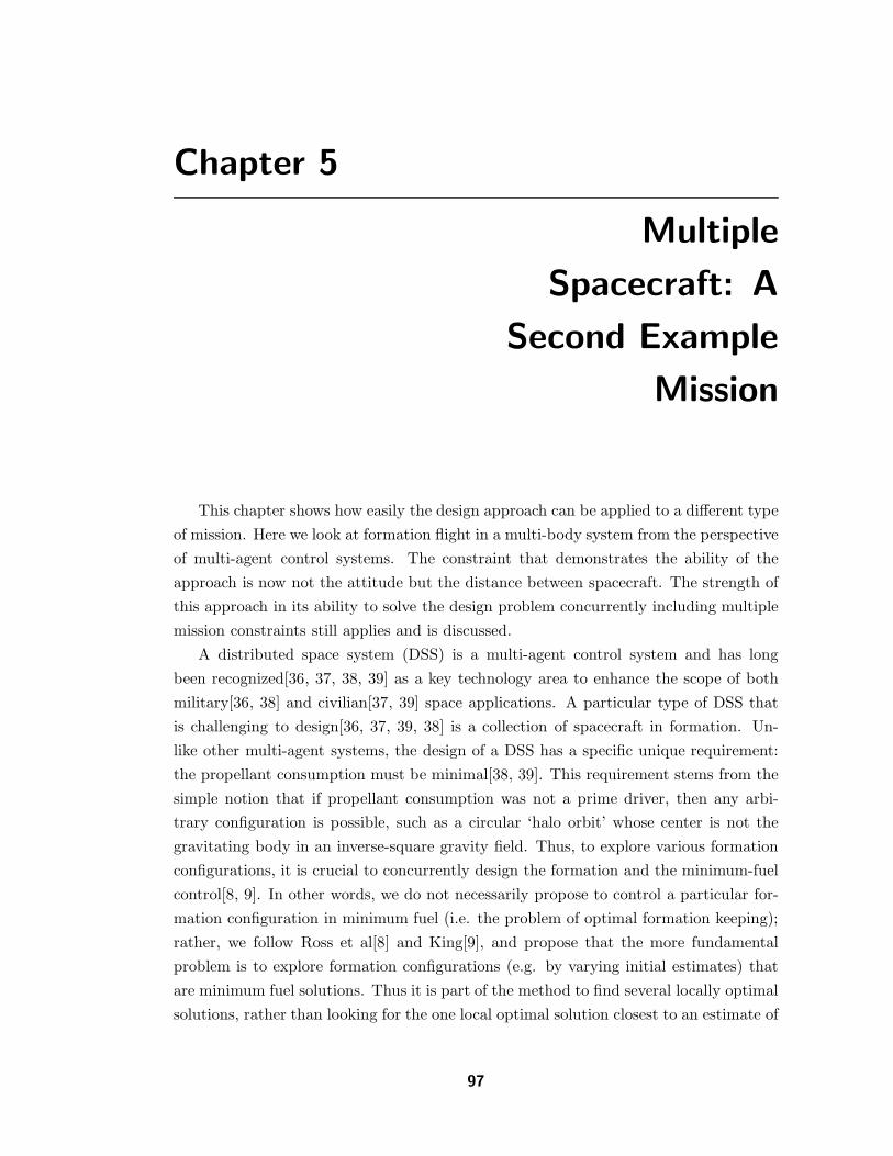
Chapter 5
Multiple
Spacecraft: A
Second Example
Mission
This chapter shows how easily the design approach can be applied to a different type
of mission. Here we look at formation flight in a multi-body system from the perspective
of multi-agent control systems. The constraint that demonstrates the ability of the
approach is now not the attitude but the distance between spacecraft. The strength of
this approach in its ability to solve the design problem concurrently including multiple
mission constraints still applies and is discussed.
A distributed space system (DSS) is a multi-agent control system and has long
been recognized[36, 37, 38, 39] as a key technology area to enhance the scope of both
military[36, 38] and civilian[37, 39] space applications. A particular type of DSS that
is challenging to design[36, 37, 39, 38] is a collection of spacecraft in formation. Un-
like other multi-agent systems, the design of a DSS has a specific unique requirement:
the propellant consumption must be minimal[38, 39]. This requirement stems from the
simple notion that if propellant consumption was not a prime driver, then any arbi-
trary configuration is possible, such as a circular ‘halo orbit’ whose center is not the
gravitating body in an inverse-square gravity field. Thus, to explore various formation
configurations, it is crucial to concurrently design the formation and the minimum-fuel
control[8, 9]. In other words, we do not necessarily propose to control a particular for-
mation configuration in minimum fuel (i.e. the problem of optimal formation keeping);
rather, we follow Ross et al[8] and King[9], and propose that the more fundamental
problem is to explore formation configurations (e.g. by varying initial estimates) that
are minimum fuel solutions. Thus it is part of the method to find several locally optimal
solutions, rather than looking for the one local optimal solution closest to an estimate of
97

98 Chapter 5 Multiple Spacecraft: A Second Example Mission
a particular formation configuration. Once this problem is solved, the next step would
be to evaluate the formation configurations for science or military applications, modify
the requirements if necessary, re-solve the problem and re-evaluate the result in con-
junction with the propellant expenditures to determine its viability[8]. This approach,
of telling agents what to do, rather than how to do it, has been successfully applied
for the design and control of a variety of Earth-orbiting formations[8, 9] and station-
keeping of libration-point missions[19]. In this paper, we extend the results of Infeld
and Murray[19] by adopting the approach of Ross and King[8, 9].
Research on formation at libration points is motivated primarily by the opportu-
nity to create the effect of larger telescopes with a precise formation of smaller tele-
scopes. Currently in design are infrared interferometry missions NASA’s Terrestrial
Planet Finder[40] and ESA’s Darwin[41], as well a NASA x-ray telescope formation
mission, Constellation-X Observatory[42]. These are all located at the Sun-Earth L2
point. There are also ideas for formations spaced about a libration point orbit; more of
a constellation around the point. An example of this idea is the two satellite constella-
tion Solar Wind Satellite proposed at Sun-Earth L1 by the Department of Defense[43].
Similar to the extensive work on spacecraft formation in the two-body problem, much
of the research on the three-plus-body problem is centered around linearization about
a reference libration orbit[44, 45, 46, 47]. Thus, the problem is split into two problems:
the design of a ‘good’ reference orbit and formation control around the reference orbit.
There are number of procedures for finding a reference orbit[48, 49], many of them are
based on a Lindstedt-Poincare technique proposed by Richardson[50]. In this approach,
the perturbation method of Lindstedt is applied to the circular restricted three-body
problem with Legendre polynomials as expansion coefficients. The accuracy of this
method is then judged by comparing the results to a direct numerical integration of the
dynamical equations. This naturally leads to a procedure for improving the initial con-
ditions by shooting methods[49, 51]. Junge et al[51] describe the issues and difficulties
of this approach for real-life missions. Having determined the reference orbit in such
a manner, formation keeping methodologies can be developed by applying linear con-
trol theory to the linearized equations of motion for a neighboring orbit[46, 47]. Many
variants of this approach are actively being pursued by various researchers. While such
a two-step approach may be viable for certain missions, a simple, unified, single-step
approach to the design and control of spacecraft formations was proposed by Ross and
King[8, 9]. In this approach, the orbits and the formation control strategies are de-
signed concurrently using the framework of multi-agent optimal control theory. It will
be apparent shortly that this framework, described Sec. II, is not the same as applying
optimization techniques to compute the standard problem of impulsive trajectory cor-

5.1 General Framework 99
rection maneuvers[52]. In any case, once the problem framework is set up, the optimal
control problem it is solved by a Legendre pseudospectral method[12, 13, 14]. This
method, summarized in Sec. III, essentially allows the state, control and costate vari-
ables to be represented as a series expansion of Legendre polynomials. Thus, although
Legendre polynomials are also used, as in Richardson’s method, the pseudospectral ap-
proach is fundamentally different and resembles a Galerkin method[53]. However, unlike
a Galerkin method, all the computations in the pseudospectral method are performed
in the time domain by an equivalent representation of the unknown variables in terms
of Lagrange interpolating polynomials. The net result is that the semi-analytical frame-
work of series expansion and the computational aspects of finding the coefficients are
unified. The computational problem is reduced to a large nonlinear programming prob-
lem. Solving such large-scale problems are significantly easier today than ever before:
thanks to major advances in practical algorithms pioneered by Betts[54] and Gill et
al[16]; these algorithms promise global convergence under mild assumptions[55]. The
results of this approach are reported in Sec. V. We briefly note that global convergence
does not imply global optimality[55, 56]; we also present globally fuel-optimal solutions
in the sense that the propellant expenditures are zero.
5.1 General Framework
Suppose that we have a collection of Ns spacecraft that constitute a DSS. Let xi(t)
denote the state of the ith spacecraft at time t. This can be the usual 6-vector position-
velocity state or any other set (e.g. orbital elements). We assume that the dynamics of
the DSS is given in some coordinate system by a set of differential equations,
xi = f i(xi,ui, t;pi) i = 1 . . . Ns, (5.1)
where f i is a given function, ui is the control variable of the ith spacecraft, and pi is a
vector of (constant) design parameters. In general, the dynamics need not be given in
state-space form, as in Eq. (5.1), but for the purpose of brevity we limit our discussion
to such a vector-field approach. By defining the state and control variables as,
x = (x1, . . . ,xNs) and u = (u1, . . . ,uNs),
the dynamics of the DSS may be represented quite succinctly as,
x = f(x,u, t;p). (5.2)

100 Chapter 5 Multiple Spacecraft: A Second Example Mission
Typically, the functions f i are all the same so that f is simply Ns copies of f1. Let
d(xi,xj) be a generic distance metric (not necessarily Euclidean) between any two
spacecraft. If d(xi(t),xj(t)) is a given constant in time, ci,j , then we say we have a
frozen formation,
ci,j ≤ d(xi(t),xj(t)) ≤ ci,j ∀ t, i, j. (5.3)
By ∀ t, we mean for all t associated with the finite lifetime of the DSS whereas by
∀ i, j we mean for all spacecraft in the system. Further, from the definition of a metric,
d(xi,xj) = 0 ∀ i = j; hence, we must have ci,j = 0 ∀ i = j as a necessary condition for
feasibility. Note that Eq.(5.3) is really an equality; the reason for masquerading it as
an inequality is to define a relaxed formation as
ci,j − δi,jl ≤ d(xi(t),xj(t)) ≤ ci,j + δi,j
u ∀ t, i, j, (5.4)
where δi,jl ≥ 0 and δi,j
u ≥ 0 are lower and upper tolerances associated with the relax-
ation. When i = j, the tolerances must be zero in conformance with the definition of a
metric. Equation (5.4) generalizes Eq.(5.3) since if δi,jl = δi,j
u = 0 ∀ i, j, we recover the
representation of the frozen formation defined by Eq.(5.3).
We can define and design various configurations based on various metrics. For
example, in libration point missions, in order to generate halo orbits, there may be a
forbidden zone such as a disk of radius R centered around the libration point, y; in this
case, we define an allowable region for x as,
d(xi(t),y) ≥ R ∀ i, t.
See King[9] for an implementation of such constraints for a variety of Earth-orbiting
missions. The requirement that no two spacecraft collide may be articulated as,
d(xi(t),xj(t)) ≥ bi,j > 0 ∀ t and i 6= j.
It is apparent that all these constraints (and many more that are specific to a partic-
ular mission) can be described in terms of a generic set of a possibly large number of
inequality constraints that can be represented as,
hl ≤ h(x,u, t;p) ≤ hu. (5.5)
In this description of a formation, there is no leader or follower; rather a system of
multiple spacecraft. Thus, if any one spacecraft has an additional configuration con-

5.1 General Framework 101
straint, it would automatically transfer in some fashion to the remainder of DSS by way
of the couplings between the various equations. For example, if there was a mission
requirement to designate a particular spacecraft as a leader and designate the others as
followers, this can be easily accomplished by picking out the particular index, i, rep-
resenting the leader. Then, when the leader moves along some trajectory, t 7→ xi, the
distance metrics along with any additional path constraints, Eq.(5.5), dictate how the
remainder of the spacecraft must follow certain trajectories to meet the path constraints;
i.e., a formation. Thus, although our framework is based on a collection of DSS, it does
not exclude a leader-follower system.
As noted earlier, fuel consumption dominates any DSS design. Translating the fuel
consumption cost we had with one spacecraft into the formation context gives
Ji =
∫ tf
t0
∥
∥ui(t)∥
∥
1dt, (5.6)
where tf − t0 is the time interval of interest and ‖·‖1 is the usual l1-norm. Treating
the problem to be invariant under time translations allows us to set t0 = 0. A critical
modeling issue in the design and control of spacecraft formations is the treatment of
the horizon, tf , vis-a-vis the mission life time. Ideally, we would like to choose tf to be
equal to the mission life. Deferring a discussion of alternative choices for the horizon,
we choose the cost functional for designing the DSS to be the total fuel consumption,
J =
Ns∑
i=1
Ji =
∫ tf
t0
Ns∑
i=1
∥
∥ui(t)∥
∥
1dt. (5.7)
In certain applications, it may be necessary to require that each spacecraft in the DSS
consume the same amount of propellant. This requirement can be stipulated as the
so-called isoperimetric constraints,
Ji = Jk ∀ i, k. (5.8)
If the equal-fuel requirement is ‘soft’ as in, Ji ≈ Jk, it can be simply stipulated as an
inequality with appropriate upper and lower bounds. Likewise, the allocation of fuel
budgets can be similarly defined.
It will be apparent shortly that the problem formulation as posed so far is quite
sufficient to handle Libration point formations in the Sun-Earth system if the spacecraft
lifetime measured in terms of the duration of the formation is about a year or so as in
the Genesis Mission.[57] This is because the number of halo orbits over this duration is
about two. For a similar lifespan, the number of orbits in the two-body Earth system

102 Chapter 5 Multiple Spacecraft: A Second Example Mission
range from several hundred to thousands. To properly account for this periodicity,
we adapt Bohr’s notion of almost periodic functions[58, 59]. Under this framework[8,
60], periodicity may be exploited for an alternative problem formulation based on a
modification to optimal periodic control theory. In this problem formulation, we write[8,
60]
J =1
tf − t0
∫ tf
t0
Ns∑
i=1
∥
∥ui(t)∥
∥
1dt, (5.9)
which is a measure of fuel consumed by the DSS averaged over the time period, (tf −
t0). It is quite tempting to choose a priori this time period equal to the period of
some appropriately chosen reference orbit; however, a far better option[8] is to let this
period be free so that the problem formulation allows the determination of an optimal
time period as well. In this case tf is bound away from t0 to prevent invalid function
evaluations. As noted in Sec. I, this option tells the agents what to do rather than how
to do it. In order to facilitate the existence of a solution for this scenario, it is now
necessary to impose two additional constraints on the problem formulation:
1. The dynamical equations, Eq.(5.1), must be written in an appropriate coordinate
system that facilitates a periodic or almost periodic solution, and
2. Boundary conditions representing the almost periodic structure of the desired
solution must be included.
Thus, assuming that the the first condition is satisfied, the boundary conditions for
strict periodicity of a periodic formation can be stipulated as,
xi(t0) = xi(tf ) ∀ i. (5.10)
Two points are worth noting at this juncture: first, these conditions are not the same
as specifying standard boundary conditions because the values of xi(t0) and xi(tf ) are
unknown. Second, as briefly noted earlier, it is sufficient to stipulate all the constraints
of Eq.(5.10) as a single constraint,
xi(t0) = xi(tf ) for i = 1 (5.11)
or any other index. This is because, the path constraints will automatically enforce the
remainder of the constraints. In this context, we may designate i = 1 as the leader,
but it essentially reduces to semantics rather than a leader-follower architecture. By
relaxing the constraint represented by Eq(5.10) to,
εil ≤ xi(t0) − xi(tf ) ≤ εi
u ∀ i, (5.12)

5.2 Libration Point Formations 103
where εil and εi
u are formation design parameters, we easily stipulate a practical means
to design and control almost periodic formations[9]. It is clear from these definitions that
a frozen formation in the Euclidean metric is a periodic formation but not vice versa.
The concept of almost periodicity is not only quite practical, it has significant theoretical
advantages. See Fischer[58] for a quick review of almost periodic functions, and Junge
et al[51] for practical demonstrations of possible contradictions in applying ordinary
Floquet analysis. Deferring the details of applying this framework for Libration point
missions to Sec. IV, we note that the problem of designing and controlling spacecraft
formations can be summarized as a nonsmooth, nonlinear, multi-agent optimal control
problem.
5.2 Libration Point Formations
Remember ri = (xi, yi, zi) denote the Cartesian components of a generic spacecraft
in the barycentric frame (see Fig. 2.1) of the circular restricted three-body problem.
The spacecraft dynamical equations are well-known and given by,
ri = vi (5.13)
vi = Cvi +∂U i
∂ri+ ui, (5.14)
where
C =
(
0 −2 0
2 0 0
)
U i ≡ U(xi, yi, zi)
U(x, y, z) =x2 + y2
2+
1 − µ
rA(x, y, z)+
µ
rB(x, y, z)
r2A(x, y, z) = (x + µ)2 + y2 + z2
r2B(x, y, z) = (x + µ − 1)2 + y2 + z2.
The acceleration control ui is norm-bounded,
∥
∥ui∥
∥
∞≤ ui
max
and represents the thruster size of a particular configuration.[29] A multitude of forma-
tion options can be defined in various ways. For example, it may be necessary to keep

104 Chapter 5 Multiple Spacecraft: A Second Example Mission
the relative Euclidean distance (l2-norm) bounded according to,
ci,j2 − δi,j
l ≤∥
∥ri(t) − rj(t)∥
∥
2≤ ci,j
2 + δi,ju ∀ t, i, j (5.15)
Another option may require to bound the l∞-norm,
ci,j∞
− δi,jl ≤
∥
∥ri(t) − rj(t)∥
∥
∞≤ ci,j
∞+ δi,j
u ∀ t, i, j (5.16)
as an alternative or additional requirement.
In some complex mission geometries, metrics not based on norms may also be used.
All the conditions posed above apply to relative formation configurations. In order to
design the ensemble about a generic Lagrange point, L ∈ {L1, . . . , L5}, an allowable
zone can be defined as,
ci,Ll ≤
∥
∥ri(t) − rL
∥
∥
2≤ ci,L
u ∀ t, i,
where rL is the position vector of L. Similar to the relative configuration metrics, other
metrics or norms may also be chosen for the allowable zone.
All of the prior conditions apply to a design of the formation system. Thus there is
no leader or follower system; rather a system of distributed spacecraft. As noted before,
it is possible to transmit conditions to the entire system by stipulating conditions on any
one spacecraft. For example, to create a formation along a halo orbit, it is necessary to
specify the ‘halo conditions’ for just one spacecraft. This is also an orbit design problem
and can be designed concurrently with the formation by imposing additional conditions.
For example, if the formation system is required to be periodic, then it is necessary to
impose the periodic conditions for just one spacecraft, say
rj(t0) = rj(tf ) (5.17)
vj(t0) = vj(tf ) for j = 1. (5.18)
To generate almost periodic trajectories, these conditions
can be relaxed to give
εjr,l ≤ rj(t0) − rj(tf ) ≤ εj
r,u (5.19)
εjv,l ≤ vj(t0) − vj(tf ) ≤ εj
v,u for j = 1. (5.20)
Although the examples in the following section includes discussion of the actual con-
straints and values used in the formulation of each, the entire formulations can be seen
in the Optimization Formulation chapter (Ch.3). Here it can be seen in the context

5.3 Numerical Examples 105
of formulations for the major example mission, a single large telescope with large solar
shield.
5.3 Numerical Examples
We demonstrate our ideas for a two spacecraft system (Ns = 2); the extension of
this approach to three or more spacecraft is straightforward. Although our method
can be applied to any libration point with similar results, we choose to design and
control formations about the Sun-Earth L2 point because of the multitude of telescope
formation missions proposed at this location; thus, we have,
µ = 2.448 × 10⁻⁶
rL = (1 − µ + 0.01, 0, 0) DU
in the barycentric frame, where DU is the distance unit equal to the astronomical
unit, AU . The origin in these examples is shifted to L2 to improve variable scaling,
so rL = (0, 0, 0). Also, we chose the Euclidean distance, the maximum acceleration
and the allowable zone parameters as the design parameters. The separation parameter
between the two spacecraft is chosen to reflect the spread of an interferometry mission.
The TPF requirement is a 1km range[40]. The next generation of ‘hypertelescopes’
being explored by optical engineers[61] will use even larger baselines for resolution of
smaller objects. At 150 km, characteristics of Earth-sized planets several parsecs away
can be directly observed. At one million km, the hypertelescope will angularly resolve
neutron stars, which are hundreds of parsecs away. We choose 15 km as the separation
for our first two examples. In problem formulations with constraint dimensions this
small in comparison to the state variable size (4 orders of magnitude difference), issues
of scaling must be resolved in order to obtain optimal solutions. In the last example,
the separation is much larger, approaching one million km, which reflects the design of
a constellation of observers, similar to the SWS proposal[43], or the outer edges of the
DSS neutron star observer of the distant future.
Example 1
In the first example, we consider a fixed-horizon problem, and set tf = 3.5 timeunits(TU)
(about 205 days). The time unit is equal to the period of the rotation system, which is
the inverse of the frequency, 2π radians per year. In seeking a relaxed formation with a

106 Chapter 5 Multiple Spacecraft: A Second Example Mission
separation of 1 × 10⁻⁷ DU (about 15 km), we set the design parameters as,
ci,j2 = 1 × 10⁻⁷ DU for i 6= j (5.21)
δi,j2 = 5 × 10⁻⁶ DU for i 6= j (5.22)
uimax = 0.001 DU/TU2 ∀ i (5.23)
Ji = Jk ∀ i, k, (5.24)
where TU , the time unit is 1/(2π) of the period of the of the primary system; i.e. a
year for the Sun-Earth system. The input states and controls (the starting point for
the optimization algorithm) were found by propagating an initial state and applying
enough thrust along the x axis at the step closest to crossing the x − z plane to make
the x velocity zero at the next step. This was done for 3 maneuver and propagate
cycles, producing a trajectory tracing a little further than one ‘orbit’, and a final time
of 3.5 TU (thus the tf defined above). This set of states and controls are the input for
both spacecraft. This means the initial estimate of the solution is infeasible since the
separation is below the minimum bound. The initial state that produced the input for
this example is (in DU and DU/TU):
x(t0) = 0.0 × 10⁻³, vx(t0) = 1.0 × 10⁻³
y(t0) = 2.5 × 10⁻³, vy(t0) = −4.5 × 10⁻³
z(t0) = 1.0 × 10⁻³, vz(t0) = −1.0 × 10⁻³
To reduce the computation time, the initial state of the solution was bound to a
box of 0.001 DU on either side of the about input initial state. Periodic constraints are
not imposed but the isoperimetric constraint of equal-fuel consumption is required (Cf.
Eq. (5.24)).
As noted earlier, we used DIDO[15] with SNOPT[16] to solve the multi-agent optimal
control design problem. A solution to the problem for a choice of 100 nodes (roughly, a
99th-order Legendre polynomial) is shown in Fig. 5.1. This solution is globally optimal
because it has zero cost, i.e. J = 0 ⇔ u = 0. The trajectories show that each of the two
spacecraft appear to follow the same shaped halo-like orbit about L2, but parallel along
the path, maintaining the tolerances on the specified separation distance as shown in
Fig. 5.2. The relative orbit, i.e. the orbit of one of the spacecraft relative to the other,
is shown in Fig. 5.3. The optimal controls are all zero at each node as shown in Fig. 5.4.
The plots for the other thrusters are similar.
The claim of optimality is based on several tests[15]. One of these tests is the

5.3 Numerical Examples 107
−10
−8
−6
−4
−2
0
2
x 10−3
−2−1
01
2
x 10−3
−1
0
1
2
x 10−3
X
Optimal Trajectories
Y
Z
s/c 1s/c 2L2Earth
Figure 5.1 Trajectories for a two-agent DSS
approximate constancy of the Hamiltonian with an average value equal to zero.[13] The
non-zero values of the Hamiltonian for this example are trivially small as shown in
Fig. 5.5. In order to practically demonstrate the convergence of the solution, we use the
optimal initial conditions (in DU and DU/TU),
x1(t0) = −0.43 × 10⁻³, v1x(t0) = 2.00 × 10⁻³
y1(t0) = 1.52 × 10⁻³, v1y(t0) = −4.30 × 10⁻³
z1(t0) = 1.93 × 10⁻³, v1z(t0) = −0.15 × 10⁻³
(x2(t0) is the required 1× 10⁻⁷DU away in position, and has similarly small differences
in velocity) to propagate the solutions using ode45 in Matlab. Fig. 5.6 shows a com-
parison of the optimized states to the propagated states of one of the spacecraft. It is
apparent that the propagated states track fairly well to the optimized ones indicating
that the 100 node solution is a good solution over this time period for preliminary de-
sign considerations. The timestep at which the solution diverges from the propagated

108 Chapter 5 Multiple Spacecraft: A Second Example Mission
0 0.5 1 1.5 2 2.5 3 3.5 40.4
0.6
0.8
1
1.2
1.4
1.6
1.8x 10
−7
Normalized Time
Distance Between Spacecraft
Figure 5.2 Separation between the two spacecraft over time
trajectory increases proportionally to the number of nodes.
Example 2
Having obtained a zero-cost solution in Example 1, we now consider the same prob-
lem with the addition of periodicity constraints. As explained in Sec. II, perodicity in
the states is imposed under a free horizon, tf ; thus, we now have,
ci,j2 = 1 × 10⁻⁷ DU for i 6= j (5.25)
δi,j2 = 5 × 10⁻⁶ DU for i 6= j (5.26)
uimax = 0.001 DU/TU2 ∀ i (5.27)
Ji = Jk ∀ i, k (5.28)
xi(t0) = xi(tf ) for i = 1. (5.29)
The input states and controls for this example were the optimal states and controls
of the first example. The initial state of the solution was again bound to a box of

5.3 Numerical Examples 109
−10
−5
0
x 10−8
−5
0
5
x 10−8
−1
−0.5
0
0.5
1
x 10−7
Relative Orbit
Figure 5.3 Relative orbit for the two-agent DSS
0.001 DU on either side, but only the positions were bound so that the initial velocities
were totally free variables. This input trajectory is shown along with the optimal
trajectories in Fig. 5.8, which is a zoomed in and stetched view of Fig. 5.7 Nevertheless,
the trajectory plots illustrate that the solution to this problem is substantially different
from that of Example 1. To properly illustrate the shape of this orbit, the trajectory in
y-z plane is plotted in Fig. 5.9 with y-axis stretched appropriately. The optimal period,
tf , for this design configuration was 3.18 TU, or 185 days. This solution is also globally
optimal because J ≈ 0. That u is almost zero (well within numerical tolerances) is
shown in Fig. 5.10 for one of the thrusters. The plots for the other thrusters are similar.
The trajectories show that each of the two spacecraft appear to follow the same
orbit about L2, but parallel along the path, maintaining the tolerances on the specified
separation distance as shown in Fig. 5.11. The relative orbit is shown in Fig. 5.12. A
clearer picture of the satisfaction of the periodicity constraints is illustrated in Fig.s 5.13
and 5.14. The circles in Fig. 5.13 are the initial and final (x, y, z). In Fig. 5.14 they mark
the initial and final (vx, vy, vz). The velocity plot shows only the data for spacecraft one
for clarity. Of course, xi(t0) does not exactly equal xi(tf ), but the differences are all
around 1× 10⁻⁷ DU, with the largest difference occurring in the z velocities of 2× 10⁻⁶
DU. These are physically small enough compared to the orbital dimension of about

110 Chapter 5 Multiple Spacecraft: A Second Example Mission
0 0.5 1 1.5 2 2.5 3 3.5
−1.5
−1
−0.5
0
0.5
1
1.5
x 10−3 X thrust
Normalized Time
s/c 1s/c 2
Figure 5.4 Thrust along the x axis for the two-agent DSS
0.002 DU to confirm that the set feasibility tolerances for the optimization algorithm
make sense.
The Hamiltonian plot in Fig. 5.15 shows that this is an optimal solution because of
its average value of zero.
We demonstrate the convergence of this large-baseline solution by propagating a
trajectory from the optimal initial conditions (in DU and DU/TU),
x1(t0) = −0.78 × 10⁻³, v1x(t0) = 0.23 × 10⁻³
y1(t0) = 0.03 × 10⁻³, v1y(t0) = 0.05 × 10⁻³
z1(t0) = 1.86 × 10⁻³, v1z(t0) = −2.53 × 10⁻³
(x2(t0) is the required 1× 10⁻⁷DU away in position, and has similarly small differences
in velocity), using ode45 in Matlab. Fig. 5.16 shows a comparison of the optimized states
to the propagated states of one of the spacecraft. It is apparent that the propagated
states track fairly well to the optimized ones indicated that the 100 node solution is a
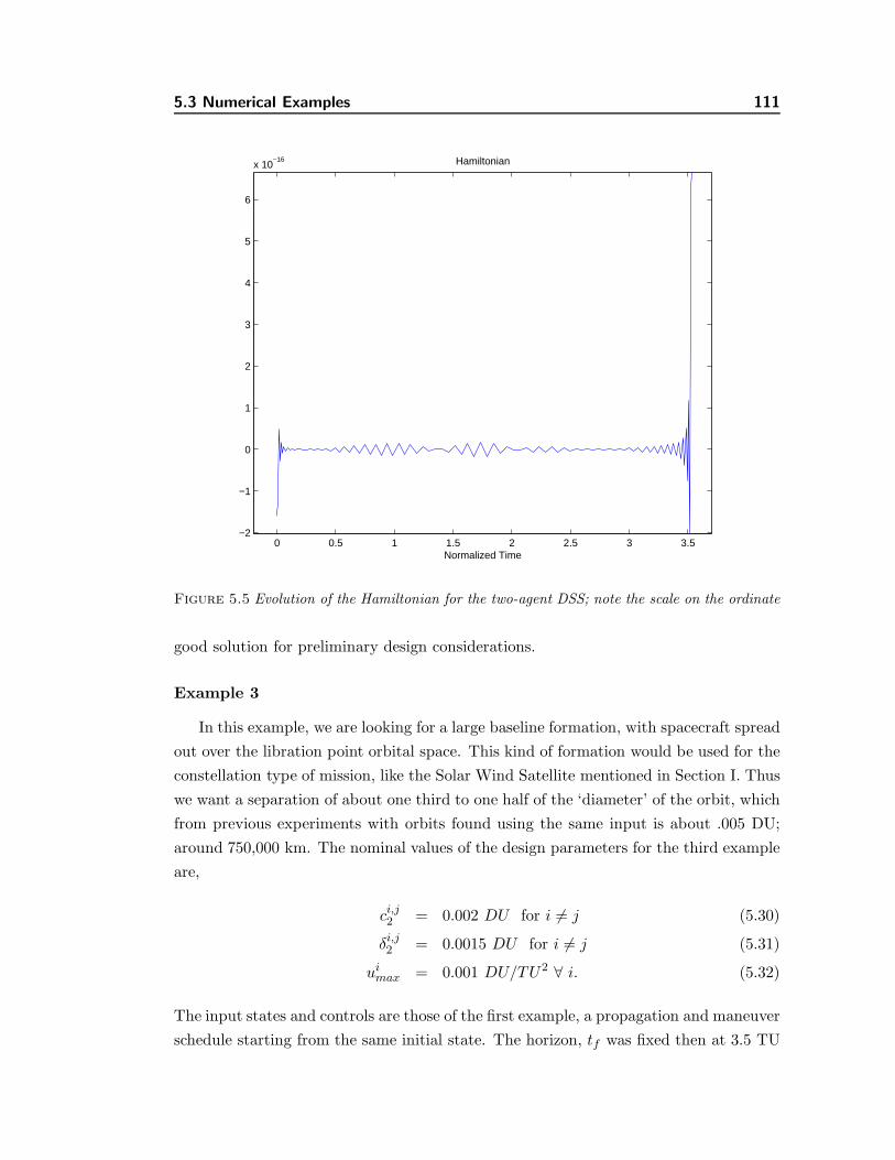
5.3 Numerical Examples 111
0 0.5 1 1.5 2 2.5 3 3.5−2
−1
0
1
2
3
4
5
6
x 10−16 Hamiltonian
Normalized Time
Figure 5.5 Evolution of the Hamiltonian for the two-agent DSS; note the scale on the ordinate
good solution for preliminary design considerations.
Example 3
In this example, we are looking for a large baseline formation, with spacecraft spread
out over the libration point orbital space. This kind of formation would be used for the
constellation type of mission, like the Solar Wind Satellite mentioned in Section I. Thus
we want a separation of about one third to one half of the ‘diameter’ of the orbit, which
from previous experiments with orbits found using the same input is about .005 DU;
around 750,000 km. The nominal values of the design parameters for the third example
are,
ci,j2 = 0.002 DU for i 6= j (5.30)
δi,j2 = 0.0015 DU for i 6= j (5.31)
uimax = 0.001 DU/TU2 ∀ i. (5.32)
The input states and controls are those of the first example, a propagation and maneuver
schedule starting from the same initial state. The horizon, tf was fixed then at 3.5 TU

112 Chapter 5 Multiple Spacecraft: A Second Example Mission
0 0.5 1 1.5 2 2.5 3 3.5 4−3
−2
−1
0
1
2
3x 10
−3 Optimal States vs. ODE Propagation
TU
DU
X
Z
Y
Figure 5.6 Comparison of the position states of spacecraft one (solid) to those propagated byODE45 in Matlab (dotted)
. No periodicity constraints were imposed, and the initial states were all free with no
bounds, however there were bounds on the positions of ±5× 10⁻³, which was an active
constraint at a few time steps for the x coordinate.
A solution to the problem for the choice of parameters listed above is shown in
Fig. 5.17. This solution again is globally optimal because it has zero cost, i.e. J = 0 ⇔
u = 0. The trajectories show that each of the two spacecraft appear to follow distinct
halo-like orbits about L2 maintaining the tolerances on the specified separation distance
as shown in Fig. 5.19. The relative orbit, i.e. the orbit of one of the spacecraft relative
to the other, is more illustrative of the configuration and is shown in Fig. 5.20.
The Hamiltonian plot in Fig. 5.21 shows that this is an optimal solution because of
its average value of zero. We demonstrate the convergence of this large-baseline solution

5.3 Numerical Examples 113
−0.01
−0.009
−0.008
−0.007
−0.006
−0.005
−0.004
−0.003
−0.002
−0.001
0
−2
−1.5
−1
−0.5
0
0.5
1
1.5
2
x 10−3
Optimal Trajectories
X
Z
Y
s/c 1s/c 2L2Earth
Figure 5.7 Trajectories for a two-agent DSS with periodicity constraints
by propagating a trajectory from the optimal initial conditions (in DU and DU/TU),
x1(t0) = −5.00 × 10⁻³, x2(t0) = −3.94 × 10⁻³
y1(t0) = 1.94 × 10⁻³, y2(t0) = 0.71 × 10⁻³
z1(t0) = 2.72 × 10⁻³, z2(t0) = 2.09 × 10⁻³
v1x(t0) = 12.74 × 10⁻³, v2
x(t0) = 10.55 × 10⁻³
v1y(t0) = 3.50 × 10⁻³, v2
y(t0) = −2.30 × 10⁻³
v1z(t0) = 7.88 × 10⁻³, v2
z(t0) = 10.54 × 10⁻³
(note x2(t0) is the required distance away from x1(t0) of 0.002) using ode45 in Matlab.
Fig. 5.22 shows a comparison of the optimized states to the propagated states of one
of the spacecraft. It is apparent that the propagated states track fairly well to the
optimized ones indicated that the 100 node solution is a good solution for preliminary
design considerations.

114 Chapter 5 Multiple Spacecraft: A Second Example Mission
−1−0.8
−0.6−0.4
−0.20
x 10−3
−6
−4
−2
0
2
4
6
x 10−4
−3
−2
−1
0
1
2
3
x 10−3
XY
Z
inputs/c 1s/c 2L2
Figure 5.8 Input and Optimal Trajectories for a two-agent DSS with periodicity constraints.NOT TO SCALE: stretched to show orbit shape
5.4 Framework for Spacecraft Formations
Because there is no linearization in this framework, we can use the same technique
and inputs for both small and large baseline formations, and find globally optimal (zero-
cost) solutions for both with entirely different trajectories. We can limit our results
as needed to find specific types of formations by including different constraints (e.g.
periodic conditions). This framework has this flexibility in applications with a simple
consistent problem formation process because the design and control are approached
concurrently.

−5 −4 −3 −2 −1 0 1 2 3 4 5
x 10−5
−2.5
−2
−1.5
−1
−0.5
0
0.5
1
1.5
2
2.5x 10
−3
−Y
Z
2D Optimal Trajectory − view from Earth
Figure 5.9 Trajectories on the y-z plane for a two-agent DSS with periodicity constraints. NOTTO SCALE: stretched along the y axis
0 0.5 1 1.5 2 2.5 3 3.5−4
−2
0
2
4
6
8
10
12
14x 10
−6 X thrust
Normalized Time
s/c 1s/c 2
Figure 5.10 Thrust along the x axis for the periodic two-agent DSS.
115

116 Chapter 5 Multiple Spacecraft: A Second Example Mission
0 0.5 1 1.5 2 2.5 3 3.50.4
0.6
0.8
1
1.2
1.4
1.6
1.8x 10
−7
Normalized Time
Distance Between Spacecraft
Figure 5.11 Separation between the two spacecraft over time

5.4 Framework for Spacecraft Formations 117
−1
−0.5
0
0.5
1
x 10−7
−10
−5
0
5
x 10−8
−6
−4
−2
0
2
4
6
x 10−8
Relative Orbit
Figure 5.12 Relative orbit for the periodic two-agent DSS

118 Chapter 5 Multiple Spacecraft: A Second Example Mission
−8
−7.9
−7.8
−7.7
−7.6
x 10−42
3
4
5
x 10−5
1.845
1.85
1.855
1.86
1.865
1.87
1.875
1.88
x 10−3
X
Position Periodic Conditions, zoomed to 1% of orbit size
Y
Z
Figure 5.13 The values of the position half of xi(t0) and xi(tf ) for i = 1, 2 are marked withcircles on this close-up view of the trajectory where it starts and ends.

5.4 Framework for Spacecraft Formations 119
2
2.2
2.4
2.6
x 10−4
2
4
6
8
10
x 10−5
−2.58
−2.57
−2.56
−2.55
−2.54
−2.53
−2.52
−2.51
−2.5
−2.49
x 10−3
Vx
Velocity Periodic Conditions: zoomed to 1% of max. velocity range
Vy
Vz
Figure 5.14 The values of the velocity half xi(t0) and xi(tf ) for i = 1 are marked with circleson this close-up view of the velocity trajectory start and end.

120 Chapter 5 Multiple Spacecraft: A Second Example Mission
0 0.5 1 1.5 2 2.5 3 3.5−0.015
−0.01
−0.005
0
0.005
0.01
0.015Hamiltonian
Normalized Time
Figure 5.15 Evolution of the Hamiltonian for the periodic two-agent DSS

5.4 Framework for Spacecraft Formations 121
0 0.5 1 1.5 2 2.5 3 3.5−2.5
−2
−1.5
−1
−0.5
0
0.5
1
1.5
2
2.5x 10
−3
TU
DU
Optimal States vs. ODE Propagation
Figure 5.16 Comparison of the position states of spacecraft one (solid) to those propagated byODE45 in Matlab(dotted)

122 Chapter 5 Multiple Spacecraft: A Second Example Mission
−4
−2
0
x 10−3−4
−2
0
2
4
x 10−3
−3
−2
−1
0
1
2
3
4
x 10−3
X
Optimal Trajectories
Y
Z
s/c 1s/c 2L2
Figure 5.17 Trajectories for a large-baseline two-agent DSS

5.4 Framework for Spacecraft Formations 123
0 0.5 1 1.5 2 2.5 3 3.5 4−1
−0.8
−0.6
−0.4
−0.2
0
0.2
0.4
0.6
0.8
1X thrust
Normalized Time
s/c 1s/c 2
Figure 5.18 Thrust along the x axis for the large-baseline two-agent DSS; note the scale on theordinate

124 Chapter 5 Multiple Spacecraft: A Second Example Mission
0 0.5 1 1.5 2 2.5 3 3.5 41.4
1.6
1.8
2
2.2
2.4
2.6x 10
−3
Normalized Time
Distance Between Spacecraft
Figure 5.19 Separation between the two spacecraft over time

5.4 Framework for Spacecraft Formations 125
−1
0
1
x 10−3−2
−1
0
1
2
x 10−3
−2
−1.5
−1
−0.5
0
0.5
1
1.5
2
x 10−3
Relative Orbit
Figure 5.20 Relative orbit for the large-baseline two-agent DSS

126 Chapter 5 Multiple Spacecraft: A Second Example Mission
0 0.5 1 1.5 2 2.5 3 3.5 4−1
−0.5
0
0.5
1
1.5
2
2.5x 10
−16 Hamiltonian
Normalized Time
Figure 5.21 Evolution of the Hamiltonian for the large-baseline two-agent DSS; note the scaleon the ordinate

5.4 Framework for Spacecraft Formations 127
0 0.5 1 1.5 2 2.5 3 3.5 4−5
−4
−3
−2
−1
0
1
2
3
4
5x 10
−3 Optimal States vs. ODE Propagation
TU
DU
X
Y
Z
Figure 5.22 Comparison of the position states of spacecraft one (solid) to those propagated byODE45 in Matlab (dotted)

128 Chapter 5 Multiple Spacecraft: A Second Example Mission

Chapter 6
Conclusions and
Future Work
This thesis showed that a systems engineering approach for space mission design of
concurrently choosing the orbit and controls, and satisfying the mission constraints, is
possible with a reasonable computation time and a relatively simple process. Changing
the mission constraints, spacecraft or force models, or type of mission is also easy, and
trivial to the solving of the problem. This is a flexible approach in that the search
space for minimum-fuel trajectories is not confined to be close to a reference orbit.
This design approach brings the more sophisticated process of concurrent engineering
to entire mission design. By incorporating optimization from the beginning of the design
process we will find total designs with lower fuel requirements because of the elimination
of unnecessary assumptions about the orbit or control design. Design approaches which
make these assumptions do not find fuel-optimal designs (only fuel-optimal maneuvers
given a set orbit).
The approach was illustrated on a libration point mission because the unstable
dynamics make this a more challenging optimal control problem than Earth orbit or
interplanetary trajectory missions. Future missions at libration points will carry more
complicated and sensitive spacecraft structure and on-board instruments, and conse-
quently will require more constraints on the stationkeeping plan, as well as being more
affected by solar radiation pressure (Chapter 2). This situation illustrated the strength
of the single optimization problem approach as the complicated dynamics and sample
constraints were easily added and only improved the performance of the optimization
algorithm, due to the choice of discretization and optimization methods (Chapter 3).
Methods of optimizing mission design using existing commercial software packages
work well enough for libration point mission design optimization if the design is sequen-
tial; first finding a reference trajectory that will work and then optimizing the maneuver
(controls) history to maintain this given constraints and perturbations. Using the con-
current trajectory control design and open design space, the standard methods would
result in a discrete problem too large computationally to be of use during a mission,
129

130 Chapter 6 Conclusions and Future Work
and may not be solvable. For example, the collocation discretization requires a very fine
grid to find an minimum-fuel mission design for a significant mission length (Section
3.1.2).
The approach presented here can be applied in the future to all types of space
missions, rather than just the libration point example, to introduce the expanded op-
timization capability to general use in mission design. The current process could be
more efficiently applied to long mission lengths by subdividing the mission timeline and
having a higher level optimization problem to ensure smooth transitions between sub-
divisions; a bi-level optimization framework. For other types of missions, or even for a
similar example, the cost functional may be differently formulated. An exponential form
may allow an even larger set of constraints and inputs to result in a good solution. To
apply this approach to later steps in the design process, one can replace the equations
of motion that describe a simple model with a more sophisticated model, even including
ephemeris data, and including error probabilities. This does not change the basic prob-
lem formulation or the ease of solving the design problem with the algorithms. Finally,
the algorithms used at this time may be improved for mission design application to
increase their efficiency. Possibilities include reformulating the differentiation matrix to
make it full rank, and allowing user- defined first and second derivatives of the functions
as part of the input of the continuous problem.

Bibliography
[1] Richard H. Battin, An Introduction to the Mathematics and Methods of Astrody-
namics, AIAA Education Series, 1987, p.385-6.
[2] Robert W. Farquhar, “The Control and use of Libration-Point Satellites,” Ph.D.
Dissertation, Department of Aeronautics and Astronautics, Stanford University,
Stanford, CA, July 1968.
[3] K.C. Howell and H.J. Pernicka, “Stationkeeping Method for Libration Point Tra-
jectories,” Journal of Guidance, Control, and Dynamics, Vol. 16, No. 1, January-
February 1993, pp. 151-159.
[4] C. Sim, G. Gmez, J. Llibre, R. Martnez, and R. Rodrquez, “On the Optimal Station
Keeping Control of Halo Orbits,” Acta Astronautica, Vol. 15, No 6/7, 1987, pp.
391-397.
[5] G. Gmez, W.S. Koon, M.W. Lo, J.E. Marsden, J. Masdemont, and S.D. Ross,
“INVARIANT MANIFOLDS, THE SPATIAL THREE-BODY PROBLEM AND
SPACE MISSION DESIGN”, AAS 01-301.
[6] Steven W. Evans, Editor, “NATURAL ENVIRONMENT NEAR THE
SUN/EARTH-MOON L2 LIBRATION POINT”, Marshall Space Flight Center.
[7] Bryson, A. and Ho, Y., Applied Optimal Control, Hemisphere/Wiley, 1975.
[8] Ross, I. M., King, J. T. and Fahroo, F., “Designing Optimal Spacecraft For-
mations,” Proceedings of the AIAA/AAS Astrodynamics Conference, AIAA-2002-
4635, Monterey, CA, 5-8 August 2002.
[9] King, J. T., “A Framework for Designing Optimal Spacecraft Formations,” M. S.
Thesis, Department of Aeronautical and Astronautical Engineering, Naval Post-
graduate School, Monterey, CA, September 2002.
[10] Infeld, S., Josselyn, S., Murray, W., and Ross, I. M., “Design and Control of
Libration Point Spacecraft Formations,” AIAA Guidance, Navigation, and Control
Conference and Exhibit, Providence, RI, August 2004. AIAA2004–4786.
[11] Bryson, Jr., A. E., Dynamic Optimization. Addison-Wesley, 1999.
131

132 Bibliography
[12] Elnagar, J., Kazemi, M. A. and Razzaghi, M., “The Pseudospectral Legendre
Method for Discretizing Optimal Control Problems,” IEEE Transactions on Auto-
matic Control, Vol. 40, No. 10, 1995, pp. 1793-1796.
[13] Ross, I. M., and Fahroo, F., “Legendre Pseudospectral Approximations of Optimal
Control Problems,” Lecture Notes in Control and Information Sciences, Vol.295,
Springer-Verlag, New York, 2003.
[14] Ross, I. M. and Fahroo, F., “Pseudospectral Knotting Methods for Solving Optimal
Control Problems,” Journal of Guidance, Control and Dynamics, Vol.27, No.3,
pp.397-405, 2004.
[15] Ross, I. M. and Fahroo, F. , “User’s Manual for DIDO 2002: A MATLAB Ap-
plication Package for Dynamic Optimization,” NPS Technical Report, AA-02-002,
Department of Aeronautics and Astronautics, Naval Postgraduate School, Mon-
terey, CA, June 2002.
[16] Gill, Murray, and Saunders, “SNOPT: An SQP Algorithm for Large-Scale Con-
strained Optimization”, SIAM Journal of Optimization, Vol. 12, No. 4, pp. 979-
1006.
[17] Holmstrom, K., Goran, A. O. and Edvall, M. M., “User’s Guide for Tomlab 4.0.6,”
Tomlab Optimization, Sweden, August 2003. http://www.tomlab.biz
[18] Analytical Graphics’ Satellite Tool Kit homepage http://www.stk.com
[19] Infeld, S. I. and Murray, W., “Optimization of Stationkeeping for a Libration Point
Mission,” AAS Space Flight Mechanics Meeting, Maui, HI, February 2004. AAS 04-
150.
[20] Howell, K.C., B.T. Barden, and M.W. Lo, “Application of Dynamical Systems
Theory to Trajectory Design for a Libration Point Mission,” The Journal of Astro-
nautical Sciences, Vol. 45, No. 2, April-June, 1997, pp.161-178.
[21] Strizzi, J. D., Kutrieb, J. M., Damphousse, P.E., Carrico, J. P., “Sun-Mars Libra-
tion Points and Mars Mission Simulations,” AAS , 2001. AAS 01-159.
[22] Wilson, R. S., “Trajectory Design in the Sun-Earth-Moon Four Body Problem,”
Ph.D. Dissertation, Department of Aeronautics and Astronautics, Purdue Univer-
sity, West Lafayette, IN, December 1998.

Bibliography 133
[23] Folta, D. and Beckman, M., “Libration Orbit Mission Design: Applications Of
Numerical And Dynamical Methods,” Libration Point Orbits and Applications,
Girona, Spain, June 2002.
[24] D.L. Richardson and N.D. Cary, “A Uniformly Valid Solution for Motion About the
Interior Libration Point of the Perturbed Elliptic-Restricted Problem,” AIAA/AAS
Astrodynamics Specialists Conference, Nassau, Bahamas, July 1975. AAS 75-021.
[25] K. C. Howell and H. J. Pernicka, “Numerical Determination of Lissajous Trajec-
tories in the Restricted Three-Body Problem,” Celestial Mechanics, Vol. 41, 1988,
pp. 107-124.
[26] Beckman, M., “James Webb Space Telescope Flight Dynamics Analysis Report,”
Flight Dynamics Analysis Branch, NASA Goddard Space Flight Center, May 2004.
[27] Barden, B. T., Wilson, R. S., Howell, K. C., and Marchand, B. G., “Summer Launch
Options for the Genesis Mission,”AAS/AIAA Astrodynamics Specialist Conference,
Quebec City, Canada, August 2001. AAS 01-306.
[28] Whiffen, G. J., “An Investigation of a Jupiter Galilean Moon Orbiter Trajectory,”
AAS 03-544.
[29] Ross, I. M., “How to Find Minimum-Fuel Controllers,” Proceedings of the AIAA
Guidance, Navigation and Control Conference, Providence, RI, August 2004. AIAA
Paper No. 2004-5346.
[30] Williams, P., “A Comparison of Differentiation and Integration Based Direct Tran-
scription Methods,”AAS/AIAA Space Flight Mechanics Conference, Copper Moun-
tain, CO, January 2005. AAS 05-128.
[31] De Miguel, V., “The Solution of Optimal Control Problems by Discretization Meth-
ods,” Qualifying Tutorial Report, Department of Engineering Economic Systems
and Operations Research, Stanford University, 2000.
[32] Stanford Business Software Inc., distributor of software produced by Systems Op-
timization Laboratory, Stanford University, Stanford, CA and University of Cali-
fornia at San Diego, La Jolla, CA. http://www.sbsi-sol-optimize.com/
[33] Gill, Murray, and Wright, Practical Optimization, Academic Press, 1986, p. 54.
[34] GESOP – Software User Manual, 2002, Institute of Flight Mechanics and Control,
University of Stuttgart, 70550 Stuttgart, Germany. http://gesop.de

134 Bibliography
[35] I. M. Ross and F. Fahroo, “Legendre Pseudospectral Approximations of Optimal
Control Problems,” Lecture Notes in Control and Information Sciences, Springer-
Verlag, 2003.
[36] New World Vistas, Summary Volume, USAF Scientific Advisory Board, December
1995.
[37] Vincent, M. A. and Bender, P. L., “The Orbital Mechanics of a Space-Borne Grav-
itational Wave Experiment,” Advances in the Astronautical Sciences, Astrodynam-
ics, 1987, Vol. 65, Part II, Pg. 1346. Edited by Soldner, J.K. et al. Paper AAS
87-523. Full paper in AAS Microfiche Series, Vol.55.
[38] Ross, I. M., “A Mechanism for Precision Orbit Control With Applications to For-
mation Keeping,” Journal of Guidance, Control and Dynamics, Vol.25, No. 4, 2002,
pp. 818-820.
[39] Carpenter, R. J., Leitner, J. A., Folta, D. C. and Burns, R. D., “Benchmark Prob-
lems for Spacecraft Formation Flying Missions,” Proceedings of the AIAA Guid-
ance, Navigation and Control Conference, Austin, TX, August 2003, AIAA 2003-
5364.
[40] Lindensmith, C. A., editor, “Technology Plan for the Terrestrial Planet Finder ”,
JPL Publication 03-007, 2003
[41] Fridlund, C.V.M., “Darwin - The Infrared Space Interferometry Mission,” ESA
Bulletin, 01 Aug 2000, Vol. 103, pp. 20-25
[42] Constellation X homepage http://constellation.gsfc.nasa.gov/
[43] National Security Space Road Map http://www.wslfweb.org/docs/roadmap/spacroad.htm
[44] Marchand, B. G. and Howell, K. C., “Formation Flight Near L1 and L2 in the Sun-
Earth/Moon Epheremis System Including Solar Radiation Pressure,” AAS/AIAA
Astrodynamics Specialist Conference, Big Sky, MT, August 2003. AAS 03-596.
[45] Hsiao, F. Y. and Scheeres, D. J., “Design of Spacecraft Formation Orbits Relative
to a Stabilized Trajectory,” AAS 03-175.
[46] Hamilton, N. H., Folta, D. and Carpenter, R., “Formation Flying Satellite Control
Around the L2 Sun-Earth Libration Point,” AIAA/AAS Astrodynamics Specialist
Conference, Monterey, CA, August 2002, AIAA 2002-4528.

Bibliography 135
[47] Gurfil, P. and Kasdin, N. J., “Dynamics and Control of Relative Motion in an Un-
stable Orbit,” AIAA/AAS Astrodynamics Conference, Denver, CO, August 2000,
AIAA 2000-4135.
[48] Gomez, G. Masdeont, J. and Simo, C., “Quasihalo Orbits Associated with Libration
Points,” Journal of the Astronautical Sciences, Vol.46, 1998, pp.135-176.
[49] Kim, M. and Hall, C. D., “Lyapunov and Halo Orbits about L2,” AAS 01-324.
[50] Richardson, D. L., “Analytic Construction of Periodic Orbits About the Collinear
Points,” Celestial Mechanics, Vol. 22, 1980, pp. 241253.
[51] Junge, O., Levenhagen, J. Seifried, A. and Dellnitz, M., “Identification of Halo
Orbits for Energy Efficient Formation Flying,” Proceedings of the International
Symposium on Formation Flying, Toulouse, France, 2002.
[52] Serban, R., Koon, W. S., Lo, M. Marsden, J. E., Petzold, L. R., Ross, S. D. and
Wilson, R. S., “Halo Orbit Mission Correction Maneuvers Using Optimal Control,”
Automatica, 38, 2002, pp.571-583.
[53] Canuto, C., Hussaini, M. Y., Quarteroni, A., and Zang, T.A., Spectral Methods in
Fluid Dynamics, Springer Verlag, New York, 1988.
[54] Betts, J. T., Practical Methods for Optimal Control Using Nonlinear Programming,
SIAM: Advances in Control and Design Series, Philadelphia, PA, 2001.
[55] Boggs, P. T. and Tolle, J. W., “Sequential Quadratic Programming,” Acta Numer-
ica, 1995, Cambridge University Press, Cambridge, UK, 1995, pp. 151.
[56] Ross, I. M., and Fahroo, F., “A Perspective on Methods for Trajectory Optimiza-
tion,” Proceedings of the AIAA/AAS Astrodynamics Conference, Monterey, CA,
August 2002. AIAA Paper No. 2002-4727.
[57] Lo, M., B. G. Williams, W. E. Bollman, D. Han, Y. Hahn, J. L. Bell, E. A. Hirst, R.
A. Corwin, P. E. Hong, K. C. Howell, B. Barden, and R. Wilson, “Genesis Mission
Design,” Paper No. AIAA 98-4468.
[58] Fischer, A., “Structure of Fourier Exponents of Almost Periodic Functions and
Periodicity of Almost Periodic Functions,” Mathematical Bohemica, No. 3, 1996,
pp. 249-262.
[59] Corduneanu, C., Almost Periodic Functions, John Wiley, New York, 1968.

136 Bibliography
[60] Ross, I. M., Yan, H. and Fahroo, F., “A Curiously Outlandish Problem in Or-
bital Mechanics,” AAS/AIAA Astrodynamics Specialist Conference, Quebec City,
Canada, July 2001, AAS-01-430.
[61] Labeyrie, A., Le Coroller, H., Dejonghe, J. , Martinache, F., Borkowski, V., Lardire,
O., Koechlin, L., “Hypertelescope imaging: from exo-planets to neutron stars,”
Proceedings of SPIE conference, vol. 4852, Hawaii, 2002.
[62] Carlson, B., Pernicka, H., and Balakrishnan, S., “Spacecraft Formation Flight
About Libration Points,” AIAA-2004-4737.
[63] Pernicka, H., Carlson, B., and Balakrishnan, S., “Discrete Maneuver Formation-
keeping at Libration Points L1 and L2,” AAS/AIAA Spaceflight Mechanics Con-
ference, Copper Mountain, CO, January 2005. AAS 05-194.
[64] McLoughlin, T. and Campbell, M., “Hybrid Leader Follower and Sensor Scheduling
for Large Spacecraft Networks,” AIAA-2004-5022.
[65] Howell, K.C. and Marchand, B.G., “Design and Control of Formations Near the
Libration Points of the Sun-Earth/Moon Ephemeris System,” GSFC Flight Me-
chanics Symposium, Greenbelt, MD, October 2003.
[66] Marchand, B.G. and Howell, K.C., “Aspherical Formations near the Libration
Points in the Sun-Earth/Moon Ephemeris System,” AAS/AIAA Space Flight Me-
chanics Meeting, Maui, HI, February 2004. AAS 04-157.
[67] Folta, D., Hartman, K., Howell, K., Marchand, B., “Formation Control of the
MAXIM L2 Libration Orbit Mission,” AIAA/AAS Astrodynamics Specialist Con-
ference, Providence, RI, August 2004.
[68] Howell, K.C. and Marchand, B.G., “Formations Near the Libration points: Design
Strategies Using Natural and Non-Natural Arcs,” GSFC 2nd International Sympo-
sium on Formation Flying Missions and Technologies, Greenbelt, MD, September
2004.
[69] Hussein, I.I., Scheeres, D.J., and Hyland, D.C., “Optimal Formation Control for
Imaging and Fuel Usage,” AAS/AIAA Spaceflight Mechanics Conference, Copper
Mountain, CO, January 2005. AAS 05-160.
[70] Luquette, R., J., and Sanner, R. M., “A non-linear approach to spacecraft formation
control in the vicinity of a collinear libration point,” AAS/AIAA Astrodynamics
Specialist Conference, Quebec City, Canada, August 2001. AAS 01-330.

Bibliography 137
[71] Gurfil, P., and Kasdin, N.J., “Dynamics and Controls of Spacecraft Formation Fly-
ing in Three-Body Trajectories”, AIAA Guidance Navigation, and Control Confer-
ence and Exhibit, Montreal, Canada, August 2001, AIAA-2001-4026
[72] Gurfil, P., Idan, M., and Kasdin, N. J., “Adaptive neural control of deep-space
formation flying,” American Control Conference, Anchorage, AK, May 2002
[73] Li, H. and Williams, T., “Formationkeeping for Sun-Earth Libration Point For-
mations by Using Solar Radiation Pressure,” AAS/AIAA Spaceflight Mechanics
Conference, Copper Mountain, CO, January 2005. AAS 05-195.
[74] Bryson, A. E. and Ho, Y.-C., Applied Optimal Control, Hemisphere Publishing
Corporation, Chapter 7, 1975.
[75] Gong, Q., Ross, I. M., Kang, W., and Fahroo, F., “Convergence of Pseudospec-
tral Methods for Constrained Nonlinear Optimal Control Problems,” Intelligent
Systems and Control, Series on Modelling, Identification and Control, Acta Press,
Calgary, Canada, 2004.
[76] Strizzi, J. Ross, I. M and Fahroo, F., “Towards real-time computation of optimal
controls for nonlinear systems,” Proceedings of the AIAA Guidance, Navigation,
and Control Conference, Monterey, CA, August 2002, AIAA Paper No. 2002-4945.