Systems Optimization Winter Semester 2015 3. Constrained ... · Systems Optimization Winter...
37
Systems Optimization Winter Semester 2015 3. Constrained Optimization Problems 3.3. Numerical Methods Dr. Abebe Geletu Technische Universit¨ at Ilmenau Institute of Automation and Systems Engineering Department of Simulation and Optimal Processes (SOP) Systems Optimization Winter Semester 2015 3. Constrained Optimization Problems TU Ilmenau
Transcript of Systems Optimization Winter Semester 2015 3. Constrained ... · Systems Optimization Winter...
Systems OptimizationWinter Semester 2015
3. Constrained Optimization Problems3.3. Numerical Methods
Dr. Abebe Geletu
Technische Universitat IlmenauInstitute of Automation and Systems Engineering
Department of Simulation and Optimal Processes (SOP)
Systems Optimization Winter Semester 2015 3. Constrained Optimization Problems
TU Ilmenau
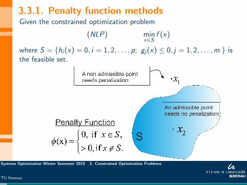
3.3.1. Penalty function methodsGiven the constrained optimization problem
(NLP) minx∈S
f (x)
where S = {hi (x) = 0, i = 1, 2, . . . , p; gj(x) ≤ 0, j = 1, 2, . . . ,m.} isthe feasible set.
Systems Optimization Winter Semester 2015 3. Constrained Optimization Problems
TU Ilmenau
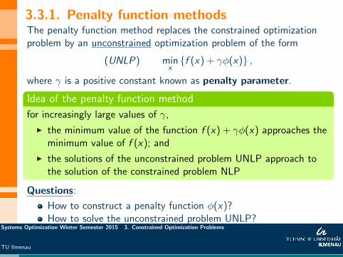
3.3.1. Penalty function methodsThe penalty function method replaces the constrained optimizationproblem by an unconstrained optimization problem of the form
(UNLP) minx{f (x) + γφ(x)} ,
where γ is a positive constant known as penalty parameter.
Idea of the penalty function method
for increasingly large values of γ,
I the minimum value of the function f (x) + γφ(x) approaches theminimum value of f (x); and
I the solutions of the unconstrained problem UNLP approach tothe solution of the constrained problem NLP
Questions:
How to construct a penalty function φ(x)?How to solve the unconstrained problem UNLP?
Systems Optimization Winter Semester 2015 3. Constrained Optimization Problems
TU Ilmenau

3.3.1. Penalty function methods ...
Requirements for a penalty function
For a function φ to be a penalty function
P1: φ(x) should be a continuous function;
P2: φ(x) ≥ 0 for all x ∈ Rn;
P3: φ(x) = 0 if and only if x ∈ S .
Any function that satisfies the properties P1-P3 can be used as apenalty function.
The penalty function should be defined in terms of S . That is,for the NLP above, it should be defined using the functionsh1, . . . , hp; g1, . . . , gm;
Thus, in the literature we find several types of penalty functions.
Systems Optimization Winter Semester 2015 3. Constrained Optimization Problems
TU Ilmenau
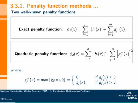
3.3.1. Penalty function methods ...Two well-known penalty functions
Exact penalty function: φ1(x) =
p∑i=1
|hi (x)|+m∑j=1
g+j (x)
Quadratic penalty function: φ2(x) =
p∑i=1
[hi (x)]2+m∑j=1
[g+j (x)
]2
where
g+j (x) = max {gj(x), 0} =
{0 if gj(x) ≤ 0,gj(x), if gj(x) > 0.
Systems Optimization Winter Semester 2015 3. Constrained Optimization Problems
TU Ilmenau
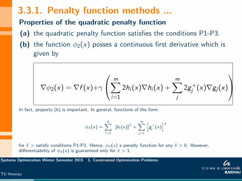
3.3.1. Penalty function methods ...Properties of the quadratic penalty function
(a) the quadratic penalty function satisfies the conditions P1-P3.
(b) the function φ2(x) posses a continuous first derivative which isgiven by
∇φ2(x) = ∇f (x)+γ
m∑i=1
2hi (x)∇hi (x) +m∑j
2g+j (x)∇gj(x)
In fact, property (b) is important. In general, functions of the form
φδ(x) =
p∑i=1
[hi (x)]δ +m∑j=1
[g+j (x)
]δ
for δ > satisfy conditions P1-P3. Hence, φδ(x) a penalty function for any δ > 0. However,differentiability of φδ(x) is guaranteed only for δ > 1.
Systems Optimization Winter Semester 2015 3. Constrained Optimization Problems
TU Ilmenau
3.3.1. Penalty function methods ...
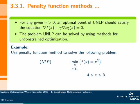
I For any given γ > 0, an optimal point of UNLP should satisfythe equation ∇f (x) + γ∇φ2(x) = 0.
I The problem UNLP can be solved by using methods forunconstrained optimization.
Example:Use penalty function method to solve the following problem.
(NLP) minx
{f (x) = x2
}s.t.
4 ≤ x ≤ 8.
Systems Optimization Winter Semester 2015 3. Constrained Optimization Problems
TU Ilmenau
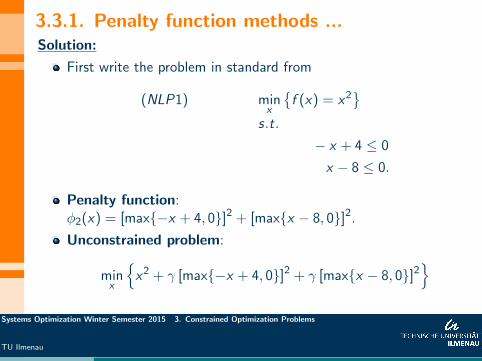
3.3.1. Penalty function methods ...Solution:
First write the problem in standard from
(NLP1) minx
{f (x) = x2
}s.t.
− x + 4 ≤ 0
x − 8 ≤ 0.
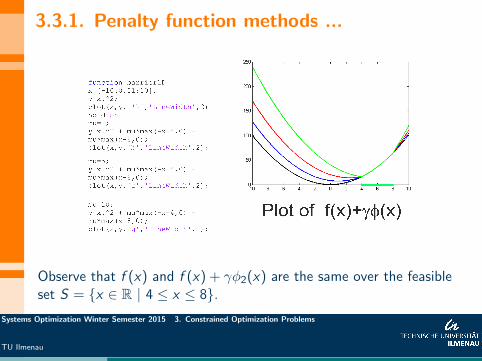
Penalty function:φ2(x) = [max{−x + 4, 0}]2 + [max{x − 8, 0}]2.
Unconstrained problem:
minx
{x2 + γ [max{−x + 4, 0}]2 + γ [max{x − 8, 0}]2
}Systems Optimization Winter Semester 2015 3. Constrained Optimization Problems
TU Ilmenau
3.3.1. Penalty function methods ...
Observe that f (x) and f (x) + γφ2(x) are the same over the feasibleset S = {x ∈ R | 4 ≤ x ≤ 8}.
Systems Optimization Winter Semester 2015 3. Constrained Optimization Problems
TU Ilmenau
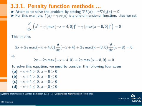
3.3.1. Penalty function methods ...I Attempt to solve the problem by setting ∇f (x) + γ∇φ2(x) = 0.I For this example, f (x) + γφ2(x) is a one-dimensional function, thus we set
d
dx
(x2 + γ [max{−x + 4, 0}]2 + γ [max{x − 8, 0}]2
)= 0
This implies
2x + 2γmax{−x + 4, 0} ddx
(−x + 4) + 2γmax{x − 8, 0} ddx
(x − 8) = 0
⇒2x − 2γmax{−x + 4, 0}+ 2γmax{x − 8, 0} = 0
To solve this equation, we need to consider the following four cases
(a) −x + 4 > 0, x − 8 > 0
(b) −x + 4 > 0, x − 8 ≤ 0
(c) −x + 4 ≤ 0, x − 8 > 0
(d) −x + 4 ≤ 0, x − 8 ≤ 0
Systems Optimization Winter Semester 2015 3. Constrained Optimization Problems
TU Ilmenau
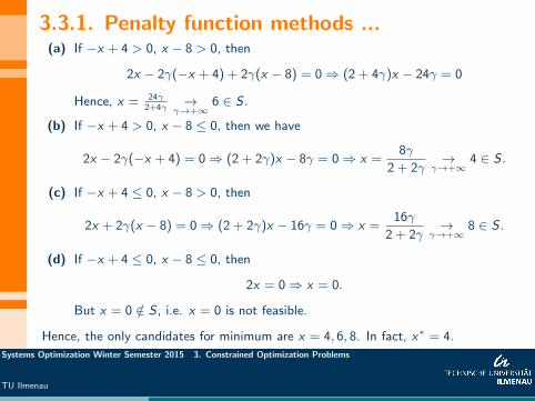
3.3.1. Penalty function methods ...(a) If −x + 4 > 0, x − 8 > 0, then
2x − 2γ(−x + 4) + 2γ(x − 8) = 0⇒ (2 + 4γ)x − 24γ = 0
Hence, x = 24γ2+4γ
→γ→+∞
6 ∈ S .
(b) If −x + 4 > 0, x − 8 ≤ 0, then we have
2x − 2γ(−x + 4) = 0⇒ (2 + 2γ)x − 8γ = 0⇒ x =8γ
2 + 2γ→
γ→+∞4 ∈ S .
(c) If −x + 4 ≤ 0, x − 8 > 0, then
2x + 2γ(x − 8) = 0⇒ (2 + 2γ)x − 16γ = 0⇒ x =16γ
2 + 2γ→
γ→+∞8 ∈ S .
(d) If −x + 4 ≤ 0, x − 8 ≤ 0, then
2x = 0⇒ x = 0.
But x = 0 /∈ S , i.e. x = 0 is not feasible.
Hence, the only candidates for minimum are x = 4, 6, 8. In fact, x∗ = 4.
Systems Optimization Winter Semester 2015 3. Constrained Optimization Problems
TU Ilmenau
3.3.1. Penalty function methods ...
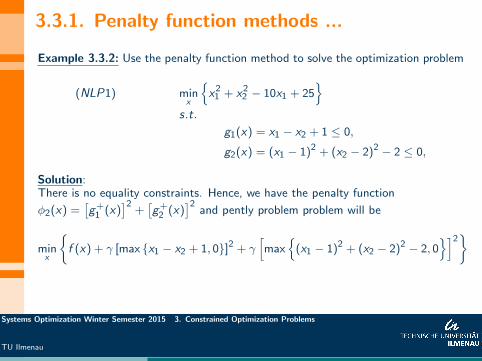
Example 3.3.2: Use the penalty function method to solve the optimization problem
(NLP1) minx
{x2
1 + x22 − 10x1 + 25
}s.t.
g1(x) = x1 − x2 + 1 ≤ 0,
g2(x) = (x1 − 1)2 + (x2 − 2)2 − 2 ≤ 0,
Solution:There is no equality constraints. Hence, we have the penalty function
φ2(x) =[g+
1 (x)]2
+[g+
2 (x)]2
and pently problem problem will be
minx
{f (x) + γ [max {x1 − x2 + 1, 0}]2 + γ
[max
{(x1 − 1)2 + (x2 − 2)2 − 2, 0
}]2}
Systems Optimization Winter Semester 2015 3. Constrained Optimization Problems
TU Ilmenau
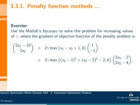
3.3.1. Penalty function methods ...
Exercise:Use the Matlab’s fminunc to solve this problem for increasing valuesof γ, where the gradient of objective function of the penalty problem is(
2x1 − 102x2
)+ 2γmax {x1 − x2 + 1, 0}
(1−1
)+ 2γmax
{(x1 − 1)2 + (x2 − 2)2 − 2, 0
}(2x1 − 22x2 − 4
).
Systems Optimization Winter Semester 2015 3. Constrained Optimization Problems
TU Ilmenau
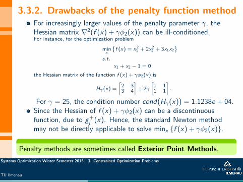
3.3.2. Drawbacks of the penalty function methodFor increasingly larger values of the penalty parameter γ, theHessian matrix ∇2(f (x) + γφ2(x)) can be ill-conditioned.For instance, for the optimization problem
minx
{f (x) = x2
1 + 2x22 + 3x1x2
}s.t.
x1 + x2 − 1 = 0
the Hessian matrix of the function f (x) + γφ2(x) is
Hγ(x) =
[2 33 4
]+ 2γ
[1 11 1
].
For γ = 25, the condition number cond(Hγ(x)) = 1.1238e + 04.Since the Hessian of f (x) + γφ2(x) can be a discontinuousfunction, due to g+
j (x). Hence, the standard Newton methodmay not be directly applicable to solve minx {f (x) + γφ2(x)}.
Penalty methods are sometimes called Exterior Point Methods.
Systems Optimization Winter Semester 2015 3. Constrained Optimization Problems
TU Ilmenau
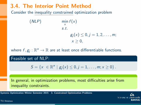
3.4. The Interior Point MethodConsider the inequality constrained optimization problem
(NLP) minx
f (x)
s.t.
gj(x) ≤ 0, j = 1, 2, . . . ,m;
x ≥ 0,
where f , gj : Rn → R are at least once differentiable functions.
Feasible set of NLP:
S = {x ∈ Rn | gj(x) ≤ 0, j = 1, . . . ,m; x ≥ 0} .
In general, in optimization problems, most difficulties arise frominequality constraints.
Systems Optimization Winter Semester 2015 3. Constrained Optimization Problems
TU Ilmenau

3.4. The Interior Point Method...
Idea of the interior point method
To iteratively approach the optimal solution from the interior of thefeasible set.
Systems Optimization Winter Semester 2015 3. Constrained Optimization Problems
TU Ilmenau
3.4. The Interior Point Method...
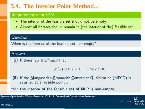
Requirements for IPMI The interior of the feasible set should not be empty.
I Almost all iterates should remain in (the interior of the) feasible set.
Question:When is the interior of the feasible set non-empty?
Answer:
(i) If there is x ∈ Rn such that
gi (x) < 0, i = 1, . . . ,m; x > 0.
(ii) If the Mangasarian-Fromovitz Constraint Qualification (MFCQ) issatisfied at a feasible point x ,
then the interior of the feasible set of NLP is non-empty.
Systems Optimization Winter Semester 2015 3. Constrained Optimization Problems
TU Ilmenau
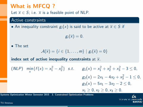
What is MFCQ ?Let x ∈ S ; i.e. x is a feasible point of NLP.
Active constraints
• An inequality constraint gi (x) is said to be active at x ∈ S if
gi (x) = 0.
• The setA(x) = {i ∈ {1, . . . ,m} | gi (x) = 0}
index set of active inequality constraints at x .
(NLP) minx{f (x) = x2
1 − x22} s.t. g1(x) = x2
1 + x22 + x2
3 − 3 ≤ 0,
g2(x) = 2x1 − 4x2 + x23 − 1 ≤ 0,
g3(x) = 5x1 − 3x2 − 2 ≤ 0,
x1 ≥ 0, x2 ≥ 0, x3 ≥ 0.Systems Optimization Winter Semester 2015 3. Constrained Optimization Problems
TU Ilmenau
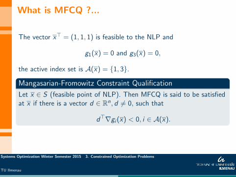
What is MFCQ ?...
The vector x> = (1, 1, 1) is feasible to the NLP and
g1(x) = 0 and g3(x) = 0,
the active index set is A(x) = {1, 3}.
Mangasarian-Fromowitz Constraint Qualification
Let x ∈ S (feasible point of NLP). Then MFCQ is said to be satisfiedat x if there is a vector d ∈ Rn, d 6= 0, such that
d>∇gi (x) < 0, i ∈ A(x).
Systems Optimization Winter Semester 2015 3. Constrained Optimization Problems
TU Ilmenau

What is MFCQ ?...
Figure: A Mangasarian-Fromowitz Vector d
• d forms an acute angle (> 900) with each ∇gi (x), i ∈ A(x).Systems Optimization Winter Semester 2015 3. Constrained Optimization Problems
TU Ilmenau
What is MFCQ ?...
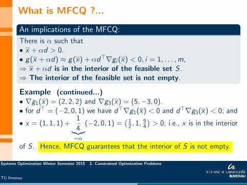
An implications of the MFCQ:
There is α such that• x + αd > 0.• g(x + αd) ≈ g(x) + αd>∇gi (x) < 0, i = 1, . . . ,m,⇒ x + αd is in the interior of the feasible set S .⇒ The interior of the feasible set is not empty.
Example (continued...)• ∇g1(x) = (2, 2, 2) and ∇g3(x) = (5,−3, 0).• for d> = (−2, 0, 1) we have d>∇g1(x) < 0 and d>∇g3(x) < 0; and
• x = (1, 1, 1) +1
4︸︷︷︸=α
(−2, 0, 1) =(
12 , 1,
54
)> 0; i.e., x is in the interior
of S . Hence, MFCQ guarantees that the interior of S is not empty.
Systems Optimization Winter Semester 2015 3. Constrained Optimization Problems
TU Ilmenau
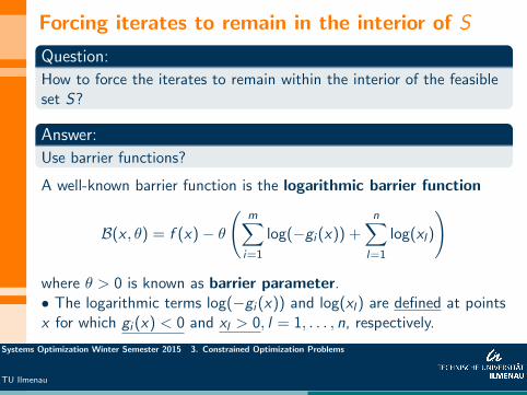
Forcing iterates to remain in the interior of S
Question:
How to force the iterates to remain within the interior of the feasibleset S?
Answer:
Use barrier functions?
A well-known barrier function is the logarithmic barrier function
B(x , θ) = f (x)− θ
(m∑i=1
log(−gi (x)) +n∑
l=1
log(xl)
)
where θ > 0 is known as barrier parameter.• The logarithmic terms log(−gi (x)) and log(xl) are defined at pointsx for which gi (x) < 0 and xl > 0, l = 1, . . . , n, respectively.
Systems Optimization Winter Semester 2015 3. Constrained Optimization Problems
TU Ilmenau
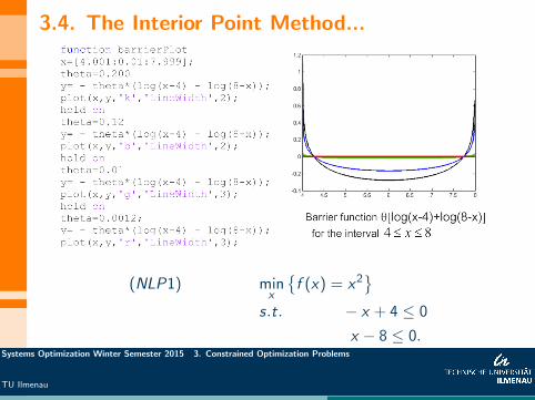
3.4. The Interior Point Method...
(NLP1) minx
{f (x) = x2
}s.t. − x + 4 ≤ 0
x − 8 ≤ 0.Systems Optimization Winter Semester 2015 3. Constrained Optimization Problems
TU Ilmenau
3.4. The Interior Point Method...Now, instead of the inequality constrained problem NLP, consider theunconstrained optimization problem
(NLP)θ minxB(x , θ)
If the original NLP has equality constraints hi (x) = 0, i = 1, . . . , p,consider the problem
(NLP)θ minxB(x , θ)
s.t.
hi (x) = 0, i = 1, 2, . . . , p.
I Generally, equality constraints do not pose difficulties. They do not needbarrier functions.
Idea of IPMI Solve the optimization problem (NLP)θ for decreasing value of θ to
obtain x(θ).
I If θ → 0+, then x(θ)→ x∗ and x∗ is a minimum point of NLP.
Systems Optimization Winter Semester 2015 3. Constrained Optimization Problems
TU Ilmenau
3.4. The Interior Point Method...• To find an optimal solution x(θ) of (NLP)θ for a fixed value of thebarrier parameter θ.
Lagrange function of (NLP)θ:
Lθ(x , λ) = f (x)− θ
m∑j=1
log(−gj(x)) +n∑
l=1
log(xl)
+
p∑i=1
λihi (x).
Necessary optimality (Karush-Kuhn-Tucker) condition:
For a given θ > 0, a vector x(θ) is a minimum point of (NLP)θ if thereis a Lagrange parameter λ(θ) such that, the pair (x(θ), λ(θ)) satisfies:
∇λLθ(x , λ) = 0
∇xLθ(x , λ) = 0
Systems Optimization Winter Semester 2015 3. Constrained Optimization Problems
TU Ilmenau
3.4. The Interior Point Method...
⇒ Thus we need to solve the system
h(x) = 0
∇f (x)− θ
m∑j=1
1
gj(x)∇gj(x) +
p∑l=1
1
xlel
+
p∑i=1
λi∇hi (x) = 0
• Commonly, this system is solved iteratively using the Newton Method.Newton method to solve the system of nonlinear equationsFθ(x , λ) = 0 for a fixed θ, where
Fθ(x , λ) =
(h(x)
∇f (x)− θ(∑m
j=11
gj (x)∇gj(x) +∑n
l=11xlel)
+∑p
i=1 λi∇hi (x)
)
Systems Optimization Winter Semester 2015 3. Constrained Optimization Problems
TU Ilmenau

3.4. The Interior Point Method...So we need to solve the equation Fθ(x , λ) = 0 for decreasing positivevalues of θ. Let JFθ(xk, λk) be the Jacobian matrix of Fθ(x , λ).
Algorithm 1: Newton Algorithm for Primal Interior Point Method
1: Choose initial iterate x(0) and λ(0);2: Choose initial step length α0;3: Choose an initial barrier parameter θ0 ;4: Select a termination tolerance tol ;5: Set k ← 0;
6: Evaluate Fθk (x(k), λ(k)) ;
7: while (∥∥Fθk (x(k), λ(k))
∥∥ > tol) do
8: Determine d = (∆kx ,∆
kλ) by solving the linear system
JFθk(x(k), λ(k))d = −Fθk (x(k), λ(k));
9: Update the step length αk and the barrier parameter θk ;
10: Set x(k+1) = x(k) + αk∆kx and λ(k+1) = λ(k) + αk∆k
λ ;
11: Evaluate Fθk (x(k), λ(k)) ;
12: Set k ← k + 1;13: end while
Systems Optimization Winter Semester 2015 3. Constrained Optimization Problems
TU Ilmenau
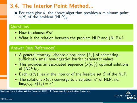
3.4. The Interior Point Method...For each give θ, the above algorithm provides a minimum pointx(θ) of the problem (NLP)θ.
QuestionsI How to choose θ’s?I What is the relation between the problem NLP and (NLP)θ?
Answer (see References)
I A general strategy: choose a sequence {θk} of decreasing,sufficiently small non-negative barrier parameter values.
I This provides an associated sequence {x(θk)} optimal solutionsof (NLP)θk .
I Each x(θk) lies in the interior of the feasible set S of the NLP.I The solutions x(θk) converge to a solution x∗ of NLP; i.e.
limθk↘0+ x(θk) = x∗.
Systems Optimization Winter Semester 2015 3. Constrained Optimization Problems
TU Ilmenau
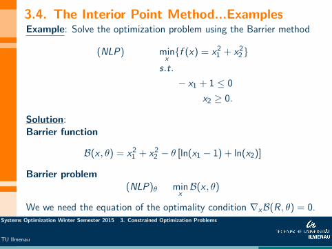
3.4. The Interior Point Method...ExamplesExample: Solve the optimization problem using the Barrier method
(NLP) minx{f (x) = x2
1 + x22}
s.t.
− x1 + 1 ≤ 0
x2 ≥ 0.
Solution:Barrier function
B(x , θ) = x21 + x2
2 − θ [ln(x1 − 1) + ln(x2)]
Barrier problem(NLP)θ min
xB(x , θ)
We we need the equation of the optimality condition ∇xB(R, θ) = 0.Systems Optimization Winter Semester 2015 3. Constrained Optimization Problems
TU Ilmenau
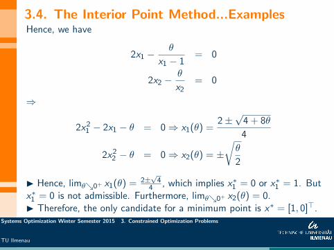
3.4. The Interior Point Method...ExamplesHence, we have
2x1 −θ
x1 − 1= 0
2x2 −θ
x2= 0
⇒
2x21 − 2x1 − θ = 0⇒ x1(θ) =
2±√
4 + 8θ
4
2x22 − θ = 0⇒ x2(θ) = ±
√θ
2
I Hence, limθ↘0+ x1(θ) = 2±√
44 , which implies x∗1 = 0 or x∗1 = 1. But
x∗1 = 0 is not admissible. Furthermore, limθ↘0+ x2(θ) = 0.I Therefore, the only candidate for a minimum point is x∗ = [1, 0]>.
Systems Optimization Winter Semester 2015 3. Constrained Optimization Problems
TU Ilmenau
3.4. The Interior Point Method...
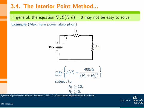
In general, the equation ∇xB(R, θ) = 0 may not be easy to solve.
Example (Maximum power absorption)
maxR1,R2
{p(R) =
400R1
(R1 + R2)2
}subject to
R1 ≥ 10,
R2 ≥ 0.Systems Optimization Winter Semester 2015 3. Constrained Optimization Problems
TU Ilmenau
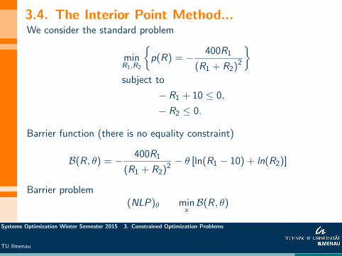
3.4. The Interior Point Method...We consider the standard problem
minR1,R2
{p(R) = − 400R1
(R1 + R2)2
}subject to
− R1 + 10 ≤ 0,
− R2 ≤ 0.
Barrier function (there is no equality constraint)
B(R, θ) = − 400R1
(R1 + R2)2− θ [ln(R1 − 10) + ln(R2)]
Barrier problem(NLP)θ min
xB(R, θ)
Systems Optimization Winter Semester 2015 3. Constrained Optimization Problems
TU Ilmenau

3.4. The Interior Point Method...
The optimality condition ∇xB(R, θ) = 0 yields the system ofnonlinear equations.
− 400
(R1 + R2)2+
800R1(R1 + R2)
(R1 + R2)3− θ
R1 − 10= 0 (1)
800R1(R1 + R2)
(R1 + R2)3− θ
R2= 0 (2)
Exercise:The system of equations above using the Newton Algorithm for adecreasing sequence of positive barrier paramters {θk}.
The interior point method discussed above is commonly known as theprimal interior point method.
Systems Optimization Winter Semester 2015 3. Constrained Optimization Problems
TU Ilmenau
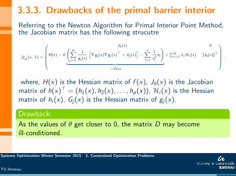
3.3.3. Drawbacks of the primal barrier interior
Referring to the Newton Algorithm for Primal Interior Point Method,the Jacobian matrix has the following strucutre
JFθ(x, λ) =
Jh(x) 0
H(x)− θ
m∑j=1
1
gj (x)
[∇gj (x)∇gj (x)> + Gj (x)
]−
n∑l=1
1
x2l
el
︸ ︷︷ ︸
:=D(x)
+∑p
i=1 λiHi (x) [Jh(x)]>
,
where, H(x) is the Hessian matrix of f (x), Jh(x) is the Jacobianmatrix of h(x)> = (h1(x), h2(x), . . . , hp(x)), Hi (x) is the Hessianmatrix of hi (x), Gj(x) is the Hessian matrix of gj(x).
Drawback:
As the values of θ get closer to 0, the matrix D may becomeill-conditioned.
Systems Optimization Winter Semester 2015 3. Constrained Optimization Problems
TU Ilmenau
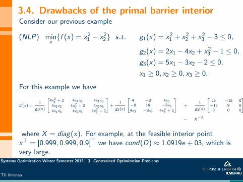
3.4. Drawbacks of the primal barrier interiorConsider our previous example
(NLP) minx{f (x) = x2
1 − x22} s.t. g1(x) = x2
1 + x22 + x2
3 − 3 ≤ 0,
g2(x) = 2x1 − 4x2 + x23 − 1 ≤ 0,
g3(x) = 5x1 − 3x2 − 2 ≤ 0,
x1 ≥ 0, x2 ≥ 0, x3 ≥ 0.
For this example we have
D(x) =1
g1(x)
4x21 + 2 4x1x2 4x1x3
4x1x2 4x22 + 2 4x2x3
4x1x3 4x2x3 4x23 + 2
+1
g2(x)
4 −8 4x3−8 16 −8x3
4x3 −8x3 4x23 + 2
+1
g3(x)
25 −15 0−15 9 0
0 0 0
− X−2
where X = diag(x). For example, at the feasible interior pointx> = [0.999, 0.999, 0.9]> we have cond(D) ≈ 1.0919e + 03, which isvery large.
Systems Optimization Winter Semester 2015 3. Constrained Optimization Problems
TU Ilmenau
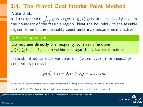
3.4. The Primal Dual Interior Point MethodNote that:• The expression 1
g(x) gets larger as g(x) gets smaller, usually near tothe boundary of the feasible region. Near the boundray of the feasibleregion, some of the inequality constraints may become nearly active.
A better approach
Do not use directly the inequality constraint functiongj(x) ≥ 0, j = 1, . . . ,m within the logarithmic barrier function.
Instead, introduce slack variables s = (s1, s2, . . . , sm) for inequalityconstraints to obtain:
gj(x) + sj = 0, sj ≥ 0, j = 1, . . . ,m.
(That is, we lift the problem into a higher dimension by adding new variables, so that we have to work with
z = (x, s) ∈ Rn+m1 . Frequently, in higher dimensions, we may have a better point of view. )
Systems Optimization Winter Semester 2015 3. Constrained Optimization Problems
TU Ilmenau
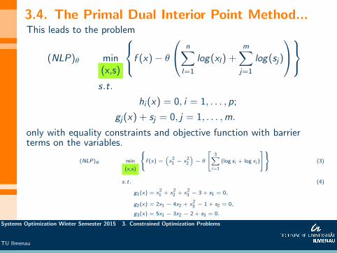
3.4. The Primal Dual Interior Point Method...This leads to the problem
(NLP)θ min(x,s)
f (x)− θ
n∑l=1
log(xl) +m∑j=1
log(sj)
s.t.
hi (x) = 0, i = 1, . . . , p;
gj(x) + sj = 0, j = 1, . . . ,m.
only with equality constraints and objective function with barrierterms on the variables.
(NLP)θ min
(x,s)
f (x) =(x2
1 − x22
)− θ
3∑i=1
(log si + log xi )
(3)
s.t. (4)
g1(x) = x21 + x2
2 + x23 − 3 + s1 = 0,
g2(x) = 2x1 − 4x2 + x23 − 1 + s2 = 0,
g3(x) = 5x1 − 3x2 − 2 + s3 = 0.
(5)Systems Optimization Winter Semester 2015 3. Constrained Optimization Problems
TU Ilmenau