Optimization of Dynamic Gait for Bipedal Robots · as constants that affect the posture of the...
6
Abstract— This paper describes a compact gait generator that runs on the on-board ATmega128 microcontroller of the Robotis Bioloid robot platform. An overview of the parameters that effect dynamic gait is included along with a discussion of how these are implemented in a servo skeleton. The gait parameters are stride height, hip swing amplitude and step period. The paper reports on the optimization of these parameters through a systematic exploration of the parameter space. The quality of the parameters is evaluated in terms of lateral head movement and foot clearance. This research was facilitated by the use of an online wireless programming interface that enables rapid testing of all the gait parameters. The gait quality was observed to be optimal at shorter step periods and larger stride heights. I. INTRODUCTION o be competitive in robot football the biped must travel quickly between one location and another. One strategy to achieve this is to have a robust dynamic gate that is stable under small perturbing external forces. This has been investigated previously in [1, 2]. The gait under investigation has no sensor feedback and thus must be highly stable to deal with the wide variety of environmental conditions, such as an uneven floor or different surface textures that will be encountered. To achieve such a gait it is important to understand the parameters that effect biped locomotion stability and to be able to optimize these parameters to suit the environment. In this paper we introduce a model of gait parameters, discuss measures of gait stability and present preliminary results for a stable dynamic gait based on the characterisation of three important dynamic properties. A bipedal humanoid platform designed at the University of Plymouth by Wolf et al. [3, 4] and based on the Bioloid servo skeleton by Robotis (Fig. 1) is used as a test bed to develop a set of parameters to optimize a dynamic gait for the FIRA 2009 RoboWorld Cup competition. II. OVERVIEW OF DYNAMIC GAIT A dynamically stable gait is one that has a repetitive motion that remains unchanged over a given time of observation or task. This means that the oscillating motion of the legs has to be inherently stable and resistant to small surface defects and changes in surface. In order to create a stable gait we first would like to be able to position the robot’s foot precisely in space. Fig. 1. University of Plymouth Biped. A. Inverse Kinematics for Positioning An inverse kinematic model of the legs of the robot is created by approximating the robots legs as a two link system for ease of computation. The accessible plane of operation for each leg is segmented into a 70x150 grid and the joint angles are pre-computed for each of these points and saved as a lookup table (Fig. 2). The lookup table is sized to occupy 2x32K and is stored in the embedded processor of the robot. When desired X (horizontal) and Y (vertical) coordinates are Optimization of Dynamic Gait for Bipedal Robots Peter Gibbons, Martin Mason, Alexandre Vicente, Guido Bugmann and Phil Culverhouse School of Computing & Mathematics, University of Plymouth Plymouth, PL4 8AA, UK [email protected] [email protected] [email protected] [email protected] [email protected]. T
Transcript of Optimization of Dynamic Gait for Bipedal Robots · as constants that affect the posture of the...
Abstract— This paper describes a compact gait generator
that runs on the on-board ATmega128 microcontroller of the
Robotis Bioloid robot platform. An overview of the
parameters that effect dynamic gait is included along with a
discussion of how these are implemented in a servo skeleton.
The gait parameters are stride height, hip swing amplitude
and step period. The paper reports on the optimization of
these parameters through a systematic exploration of the
parameter space. The quality of the parameters is evaluated
in terms of lateral head movement and foot clearance. This
research was facilitated by the use of an online wireless
programming interface that enables rapid testing of all the
gait parameters. The gait quality was observed to be optimal
at shorter step periods and larger stride heights.
I. INTRODUCTION
o be competitive in robot football the biped must travel
quickly between one location and another. One strategy
to achieve this is to have a robust dynamic gate that is
stable under small perturbing external forces. This has
been investigated previously in [1, 2]. The gait under
investigation has no sensor feedback and thus must be
highly stable to deal with the wide variety of environmental
conditions, such as an uneven floor or different surface
textures that will be encountered. To achieve such a gait it
is important to understand the parameters that effect biped
locomotion stability and to be able to optimize these
parameters to suit the environment. In this paper we
introduce a model of gait parameters, discuss measures of
gait stability and present preliminary results for a stable
dynamic gait based on the characterisation of three
important dynamic properties.
A bipedal humanoid platform designed at the
University of Plymouth by Wolf et al. [3, 4] and based on
the Bioloid servo skeleton by Robotis (Fig. 1) is used as a
test bed to develop a set of parameters to optimize a
dynamic gait for the FIRA 2009 RoboWorld Cup
competition.
II. OVERVIEW OF DYNAMIC GAIT
A dynamically stable gait is one that has a repetitive
motion that remains unchanged over a given time of
observation or task. This means that the oscillating motion
of the legs has to be inherently stable and resistant to small
surface defects and changes in surface. In order to create a
stable gait we first would like to be able to position the
robot’s foot precisely in space.
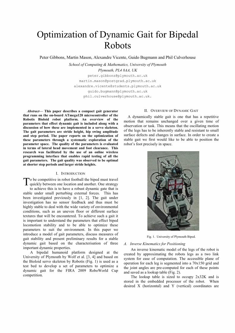
Fig. 1. University of Plymouth Biped.
A. Inverse Kinematics for Positioning
An inverse kinematic model of the legs of the robot is
created by approximating the robots legs as a two link
system for ease of computation. The accessible plane of
operation for each leg is segmented into a 70x150 grid and
the joint angles are pre-computed for each of these points
and saved as a lookup table (Fig. 2).
The lookup table is sized to occupy 2x32K and is
stored in the embedded processor of the robot. When
desired X (horizontal) and Y (vertical) coordinates are
Optimization of Dynamic Gait for Bipedal
Robots Peter Gibbons, Martin Mason, Alexandre Vicente, Guido Bugmann and Phil Culverhouse
School of Computing & Mathematics, University of Plymouth
Plymouth, PL4 8AA, UK
T

calculated from the gait driving function, the joint angles
are retrieved from the lookup table and applied to the planar
hip, knee and foot servo positions. If the hip rotates then
the kinematic plane is also rotated and the lookup table is
used to determine the servo positions.
B. Dynamic Gait Parameters
To establish the dynamic gait, a sinusoid was mapped to
the X and Y coordinates of each foot with the parameters of
stride amplitude and period. The coordinates of the first
foot are calculated by the following function:
2_ *cos( ) _
tX Stride Length X Offset
T
π= +
(1)2
_ *sin( ) _t
Y Stride Height Y OffsetT
π= +
(2)
These two functions create an ellipsoid with a
horizontal axis of two times the stride length and a vertical
axis of two times the stride height. The second foot is
mapped out of phase by π radians from the first foot. Once
the joint angles are calculated, the servo velocities are
calculated by determining the rotation angle of each servo
and then ensuring that all servos take the same time to
complete the movement. This basic sinusoidal function
serves as the building block for the dynamic gait, but a
number of other dynamic and static parameters are also
implemented.
Fig. 2. The joint angles for each of the grid points are pre-computed and stored in the onboard microprocessor. The curve indicates the trajectory of
the foot defined by (1) & (2).
C. Static Parameters
The following properties are static in that they remain
as constants that affect the posture of the robot.
1) Tilt: To maintain a stable dynamic walk, the robot’s
centre of mass should be positioned slightly forward
(Fig. 3). Depending on the geometry of the robot and its
current mass configuration, the robot should be inclined
forward by adding some additional rotation to the planar
hip servos.
Fig. 3. The tilt inclines the centre of gravity to balance the robot.
2) Body Offset: This defines how erect the robot stands
(Fig. 4). When the Y component of the foot’s position is
calculated, a constant offset is added to change the overall
height of the stance. Since the origin is defined as the foot
coordinates with the legs fully straight, without a body
offset, the calculated Y positions (equation 2) will become
negative and thus out of bounds for the inverse kinematic
model.
Fig. 4. The body offset shifts the vertical origin of the coordinate system
through which the foot moves.
3) Camber: This adds an offset to the rotational hip
servo and a mirroring offset to the rotational foot servo
(Fig. 5). With a camber of zero, the robot stands with its
legs aligned parallel. As a negative camber is added, the

legs spread outward providing a force pointing inward
which helps to increase stability.
Fig. 5. Camber introduces a rotational offset on the hip and ankle joints to
increase lateral stability and prevent collisions between servo skeleton elements.
D. Dynamic Parameters
These parameters change as a function of time during
the motion of the robot. The overall motion of the legs was
discussed previously as a sinusoidal function mapped to the
plane defined by the vector from the hip to the knee and the
vector from the knee to the ankle.
1) Swing: In order for the robot to move, it has to shift
its centre of mass from one foot to the other (Fig. 6). In this
simple implementation, a linear function is mapped to the
rotational hip servos with the same period as the sinusoid
(Fig. 7) and a mirrored function is mapped to the rotational
foot servos. This causes the robot to sway back and forth
continually shifting its centre of mass from one foot to the
other. The current implementation is not ideal and is a
remnant from decisions made during competition. We
would like to have the hip swing occur ahead of the foot
clearance to increase the mass over the foot that is to
remain planted.
Fig. 6. Swing Amplitude controls how far the centre of mass of the robot shifts.
0 1 2 3 4 5 6-1
-0.8
-0.6
-0.4
-0.2
0
0.2
0.4
0.6
0.8
1
Angle (Radians)
Relationship between foot motion and hip swing
Amplitude
Fig. 7. The relationship between the swing of the hips (straight line) and
the motion of the feet (curved line).
The following figures summarise the parameters that
determine the gait and how they are used to calculate the
servo positions.
Fig. 8. Overview of planar servo calculations
Fig. 9. Overview of Rotation Servo Calculations
III. IMPLEMENTATION
A custom firmware in a lookup table form was developed
that contains the inverse kinematics for the Bioloid Legs
and all of the functions detailed above. A windows front
end (Fig. 10) passes variables to the controller through a
wireless ZigBee serial connection. The front end allows the
user to dynamically alter all of the parameters of the model
and quickly implement new parameter values in addition to
allowing you to drive the robot remotely.
Inverse kinematic
model to calculate
planar joint angles for Hip, Knee and
Tilt gives an
offset to the
planar hip servo
Body offset is
a constant
offset to the planar knee
servo
Sinusoidal functions to generate
coordinates for
inverse kinematic model
Stride height sets Y
amplitude
Stride length sets X amplitude
Stride
period
Camber is an
offset to the rotational hip
and foot servos
Symmetric triangle waves determine the
position of the
rotational hip and foot servos
Swing sets the
X amplitude
Stride period
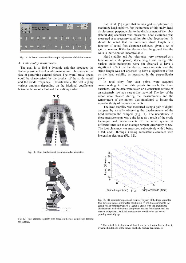
Fig. 10. PC based interface allows rapid adjustment of Gait Parameters.
A. Gate quality measurements
The goal is to find a dynamic gait that produces the
fastest possible travel while maintaining robustness in the
face of perturbing external forces. The overall travel speed
could be characterized by the product of the stride length
and the stride frequency. Unfortunately, the feet slip by
various amounts depending on the frictional coefficients
between the robot’s foot and the walking surface.
Fig. 11. Head displacement was measured as indicated.
Fig. 12. Foot clearance quality was based on the foot completely leaving
the surface.
Latt et al. [5] argue that human gait is optimized to
maximize head stability. For the purpose of this study, head
displacement perpendicular to the displacement of the robot
(lateral displacement) was measured. Foot clearance was
measured as a necessary condition for robot locomotion1. It
should be noted that the maximum stride length is a
function of actual foot clearance achieved given a set of
gait parameters. If the feet do not clear the ground then the
walk is inefficient or uncontrollable. Head stability and foot clearance were measured as a
function of stride period, stride height and swing. The
various static parameters were not observed to have a
significant effect on the desired measurements and the
stride length was not observed to have a significant effect
on the head stability as measured in the perpendicular
plane.
In total sixty four data points were acquired
corresponding to four data points for each the three
variables. All the data were taken on a consistent surface of
an extremely low nap carpet-like material. The feet of the
robot were cleaned during the measurements and the
temperature of the motors was monitored to insure the
reproducibility of the measurements.
The head stability was measured using a pair of digital
callipers by visually observing the displacements of the
head between the callipers (Fig. 11). The uncertainty in
these measurements was quite large as a result of the crude
technique and measurements of the same system at
different times led to an average percent uncertainty of 6%.
The foot clearance was measured subjectively with 0 being
a fail, and 1 through 3 being successful clearances with
increasing clearance (Fig. 12).
34
56
6
7
8
924
28
32
36
38
Swing Amplitude (4mm)Stride Height (mm)
Period (15.6 ms)
Fig. 13. 3D parameters space and results. For each of the three variables
four different values were tested resulting in 43 or 64 measurements. At each point in parameter space, a vector is drawn with the lateral head
displacement as the horizontal component and the foot clearance as the
vertical component. An ideal parameter set would result in a vector pointing vertically up.
1 The actual foot clearance differs from the set stride height dues to
dynamic limitations of the servos and body posture dependences.

IV. DATA ANALYSIS
The results are plotted in three dimensions to show
how the volume of the parameter space was investigated
(Fig. 13). At each point in the parameter space, a vector is
drawn with the lateral head displacement as the x
coordinate and foot clearance as the y coordinate. An ideal
parameter set should result in no lateral head displacement
and a non-zero foot clearance. This would be represented
by a vector pointing vertically up. Note: the head stability
measured in mm is scaled to the same range as the foot
clearance by dividing it by a scaling factor of five. No
errors are indicated but it is important to remember that
there is an average uncertainty in the length of each vector
of 6%. Each of the variables will be examined as a 2D
projection on the 3D graph (Fig. 13).
A. Period vs. Swing
Head stability shows a strong dependence on period and
an additional dependence on swing amplitude. However, at
the bottom most right of the graph (Fig. 14), the robot has
become unstable at high values of step height and fails to
achieve the necessary foot clearance for lower values. The
most promising region for further investigation is as
indicated by the ellipse.
3 3.5 4 4.5 5 5.5 6 6.5 722
24
26
28
30
32
34
36
38
Swing Amplitude (4mm)
Period (15.6 m
s)
Fig. 14. Measured Quantities as a function of Period and Hip Swing
amplitude. The multiple vectors at each point correspond to each of the measured stride heights.
B. Step Height vs. Swing Amplitude
The robot has the greatest head stability in the lower
right region of graph (Fig. 15) where the robot is not lifting
its feet off the ground. These points are not useful for a
dynamic walk since in order to walk, it must lift its feet.
Moving toward the top portion of the graph, it is clear that
both the head stability and the foot clearance are improved
by moving to larger step heights. The seemingly best values
are grouped in the region indicated by the ellipse on the
graph. This is a region calling for more detailed
investigation.
3 3.5 4 4.5 5 5.5 6 6.55.5
6
6.5
7
7.5
8
8.5
9
9.5
Swing Amplitude (4mm)
Stride Height (m
m)
Fig. 15. Measured quantities as a function of stride height and swing.
Each point contains four vectors corresponding to each of the periods.
C. Period vs. Stride Height
Here the positive effects of higher frequency on head
stability are quite apparent. However, there is a
countervailing effect that lower period leads to undesirably
lower foot clearance. Only at large values of stride height
does the robot reach acceptable values of foot clearance.
The bottom right of this graph (Fig. 16) is the most
promising region for further investigation.
6 6.5 7 7.5 8 8.5 9 9.5 1022
24
26
28
30
32
34
36
38Period (15.6 m
s)
Stride Height (mm)
Fig. 16. Measured quantities as a function of period and swing. Each point contains four vectors corresponding to each of the stride heights.
Combining the analysis shown in Fig. 14, 15 and 16, we
can indicate the bounds of the optimal head stability and
foot clearance parameter space as an ellipsoid in Fig. 17.
34
56
6
7
8
924
28
32
36
38
Swing Amplitude (4mm)Stride Height (mm)
Period (15.6 ms)
Fig. 17. Ellipsoid indicates the optimal region of parameter space for head
stability and foot clearance.

V. CONCLUSION AND FURTHER WORK
The parameters of stride height, swing and period that
were identified as being important for head stability were
each shown to have an effect on that stability as measured.
The dependence of head stability on each of these variables
was tested and a region of stable operation was identified.
The tools that were developed were useful in evaluating
gait parameters and show great promise in allowing further
investigation as we change the geometry, servos, weight
distribution etc. of the robot.
We found that operating the robot with a shorter
period, a median value for hip swing and maximizing the
step height led to increased head stabilization. Since two of
these parameters were optimal at the limits of the parameter
space explored in this study, the analysis should be
extended to include additional regions. This study was
further limited in that it used a fixed camber, body height
and tilt. Adjusting these parameters may affect the optimal
stability region for the overall robot. Preliminary
measurements of the linear speed of the robot were made
while operating in the current optimal volume of the
parameter space and the robot was able to walk for 3 meters
without falling at higher speeds than were previously
achievable (up to 0.22 ± 0.011 m/s compared with previous
maximum speeds of 0.14 ± 0.008 m/s).
In addition to further work mentioned above, the linear
ramps used for the swing should be replaced with a
function that more rapidly shifts the centre of mass over
one foot and then leaves it there until the next foot is
coming down. This would result in the centre of gravity
being over the foot for a much longer time and thus
reducing the amount of slippage that occurs as the biped
walks. During the study, the arms were held fixed parallel
to the sides of the biped. Arm oscillations can provide
additional stabilization [6] and need to be investigated.
Now that the region of stability has been identified,
additional work is required to identify the most stable point
within that region. In addition, while head stability is one
measure of overall stability, it only addresses the stability
of the robot in the axis perpendicular to the motion. The
trajectories through the parameter space that allow for
stable transitions between different locomotion speeds and
rotations need to be investigated. With the tools developed,
these additional investigations can be performed in a
methodical way and should lead to increased optimization
of the biped’s gait.
ACKNOWLEDGEMENT
The authors would like to acknowledge the valuable
contributions from Phil Hall and Joerg Wolf.
REFERENCES
[1] Mayer N, Ogino M, Guerra, R, Boedecker, J, Fuke S, Toyama H,
Watanabe A, Masui K, Asada M “JEAP Team Description”
RoboCup Symposium, 2008. [2] Behnke S, Online Trajectory Generation for Omnidirectional Biped
Walking. In Proc. of 2006 IEEE International Conference on
Robotics and Automation (ICRA'06), Orlando, Florida, pp. 1597-
1603, May 2006. [3] Wolf J, Vicente A, Gibbons P, Gardiner N, Tilbury J, Bugmann G
and Culverhouse P (2009) in Proc. FIRA RoboWorld Congress
2009, Incheon, Korea, August 16-20, 2009 (Springer Progress in Robotics: ISBN 978-3-642-03985-0) . pp. 25-33.
[4] Wolf J, Hall P, Robinson P, Culverhouse P,
"Bioloid based Humanoid Soccer Robot Design" in the Proc. of the Second Workshop on Humanoid Soccer Robots @
2007 IEEE-RAS International Conference on Humanoid Robots,
Pittsburgh (USA), November 29, 2007. [5] Latt M, Menz H, Fung V, Lord S. (2007) “Walking speed, cadence
and step length are selected to optimize the stability of head and
pelvis accelerations” Experimental Brain Research Vol 184: pp 201 – 209.
[6] Shibukawa M, Sugitani K, Kasamatsu K, Suzuki S, Ninomija S
(2001) “The Relationship Between Arm Movement and Walking Stability in Bipedal Walking” Accessed online Oct 1 2009. URL
handle.dtic.mil/100.2/ADA409793.