Optimization of Chemical Vapor Infiltration

with Simultaneous Powder Formation †

A. Ditkowski,‡ D. Gottlieb §, and B.W. Sheldon ¶

.

to appear in Journal of Materials Research

Key Words: Composites, chemical vapor deposition (CVD), Optimization, Computer

simulation, Theory.

†Research supported by DOE 98ER25346‡Division of Applied Mathematics,Brown University Providence, RI 02912§Division of Applied Mathematics Brown University Providence, RI 02912¶Division of Engineering Brown University Providence, RI 02912

ABSTRACT

A key difficulty in isothermal, isobaric chemical vapor infiltration is the long processing

times that are typically required. With this in mind, it is important to minimize infiltra-

tion times. This optimization problem is addressed here, using a relatively simple model

for dilute gases. The results provide useful asymptotic expressions for the minimum time

and corresponding conditions. These approximations are quantitatively accurate for most

cases of interest, where relatively uniform infiltration is required. They also provide useful

quantitative insight in cases where less uniformity is required. The effects of homogeneous

nucleation were also investigated. This does not effect the governing equations for infiltration

of a porous body, however, powder formation can restrict the range of permissible infiltration

conditions. This was analyzed for the case of carbon infiltration from methane.

2

I Introduction

A variety of materials are produced by infiltration processes. In these techniques a

fluid phase (i.e., a gas or a liquid) is transported into a porous structure, where it then

reacts to form a solid product. These methods are particularly important for producing

composite materials, where the initial porous perform is composed of the reinforcement phase

(i.e., fibers, whiskers, or particles) and infiltration produces the matrix [1], [2]. A detailed

assessment of the relevant reaction and mass transport rates during infiltration requires

mathematical modeling, using a minimum of two coupled partial differential equations which

describe changes in the reactant concentration and the solid structure as a function of both

position and time. This type of modeling can also be extended to analyze the optimization

and control of infiltration processes.

The research presented here specifically considers optimization for a set of two equations

which describe isothermal, isobaric chemical vapor infiltration (CVI). In this process a vapor-

phase precursor is transported into the porous preform, and a combination of gas and surface

reactions leads to the deposition of the solid matrix phase. During infiltration the formation

of the solid product phase eventually closes off porosity at the external surface of the body,

blocking the flow of reactants and effectively ending the process. This is a key feature of

most infiltration processes. Isothermal, isobaric CVI often requires extremely long times, so

it is generally important to minimize the total processing times.

This paper considers the problem of determining the optimal pressure and temperature

which correspond to the minimum infiltration time. From a practical perspective, the nature

of the porous preform is often predetermined by the intended application (e.g., the physical

dimensions and the fiber size are invariants). Thus, the process can only be controlled

with process variables: temperature, pressure, and gas composition. Note that the pressure

and temperature determine several different physical quantities in the model, such that the

general understanding of the optimum conditions is not immediately obvious from the basic

formulation.

Several previous efforts have addressed minimal infiltration times [7], [8], [9], [10], [11].

The work described here differs from these previous efforts in several ways. First, the asymp-

totic solutions obtained here make it possible to estimate the optimal conditions without

conducting detailed numerical calculations. This paper uses a relatively simple mathemati-

3

cal model which is based on the diffusion and reaction of a single, dilute precursor. However,

the numerical results which are used to verify and understand the limitations of the asymp-

totic results are generally similar to previously reported numerical results. Also, the results

presented here are based on carbon CVI from methane, in comparison with previous efforts

on CVI optimization which have emphasized SiC CVI from methyltrichlorosilane. The use

of different chemistry does not change the general conclusions obtained here, however, the

actual values do correspond to a somewhat different process. This paper also considers an

additional constraint due to homogeneous nucleation (powder formation), which has not

been treated in previous efforts. Powder formation can be significant in many CVI processes

(including carbon formation), and this effect can alter the optimal temperature and pressure

under certain conditions.

This paper is organized as follows: Section 2 presents the basic set of two partial dif-

ferential equations used to model isothermal, isobaric CVI (including initial and boundary

conditions). A definition for a successful process and a discussion on the optimization prob-

lem is given. In Section 3 an analysis of the optimization problem is given. The analysis

performed is based on asymptotic expansions as well as computations. The results of the

analysis are optimal working pressure and temperature. In Section 4 the effects of powder

formation in the analysis are included in the analysis; here too the pressure and temperature

to minimize the final time are provided. In Section 5 a discussion of the significance of these

results is presented.

II Formulation

A mathematical description of infiltration requires one or more partial differential equa-

tions which describe the evolution of the matrix (i.e., the solid phase), and one additional

partial differential equation for each chemical species in the fluid phase. For a simple pore

structure, the continuity equation for species i is

∂(εCi)

∂t+∇ ·Ni =

nr∑r

νirRr (1)

where t is time, ε is the void fraction of the media, Ci nd Ni are the concentration and the

flux of species i, nr is the number of the gaseous species, νir is the stoichiometric coefficients

for the ith gaseous species in the rth reaction, and Rr represents the volumetric reaction

rate of reaction r.

4

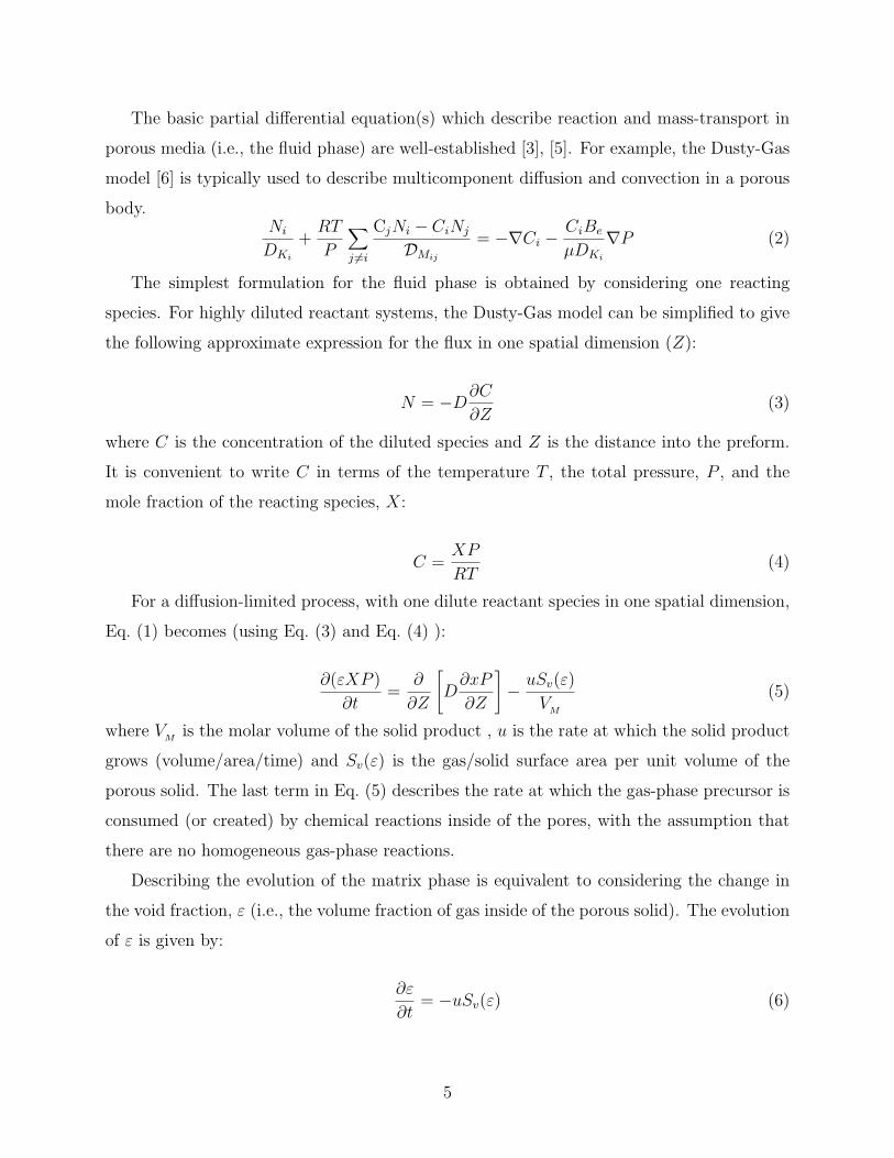
The basic partial differential equation(s) which describe reaction and mass-transport in

porous media (i.e., the fluid phase) are well-established [3], [5]. For example, the Dusty-Gas

model [6] is typically used to describe multicomponent diffusion and convection in a porous

body.Ni

DKi

+RT

P

∑

j 6=i

CjNi − CiNj

DMij

= −∇Ci − CiBe

µDKi

∇P (2)

The simplest formulation for the fluid phase is obtained by considering one reacting

species. For highly diluted reactant systems, the Dusty-Gas model can be simplified to give

the following approximate expression for the flux in one spatial dimension (Z):

N = −D∂C

∂Z(3)

where C is the concentration of the diluted species and Z is the distance into the preform.

It is convenient to write C in terms of the temperature T , the total pressure, P , and the

mole fraction of the reacting species, X:

C =XP

RT(4)

For a diffusion-limited process, with one dilute reactant species in one spatial dimension,

Eq. (1) becomes (using Eq. (3) and Eq. (4) ):

∂(εXP )

∂t=

∂

∂Z

[D

∂xP

∂Z

]− uSv(ε)

VM

(5)

where VM

is the molar volume of the solid product , u is the rate at which the solid product

grows (volume/area/time) and Sv(ε) is the gas/solid surface area per unit volume of the

porous solid. The last term in Eq. (5) describes the rate at which the gas-phase precursor is

consumed (or created) by chemical reactions inside of the pores, with the assumption that

there are no homogeneous gas-phase reactions.

Describing the evolution of the matrix phase is equivalent to considering the change in

the void fraction, ε (i.e., the volume fraction of gas inside of the porous solid). The evolution

of ε is given by:

∂ε

∂t= −uSv(ε) (6)

5

The boundary conditions most often used for CVI models are to fix the concentration at

the outer surface of the preform, and to assume that diffusion occurs in from two opposite

sides, such that there is no net flux in the middle of the preform (i.e., at Z = L, where L is

the half-thickness of the preform):

X(0, t) = Xo (7)

Xz(1, t) = 0 (8)

where z = Z/L.

The initial condition is given by:

ε(z, 0) = ε0(z) (9)

A specific CVI model requires expressions for u, Sv, and D. Our objective in this work

is to use relatively simple formulations for each, as a basis for assessing optimization during

isothermal, isobaric CVI. As an example, consider the formation of carbon matrix composites

from a mixture of CH4 in an H2 carrier gas, where the following net reaction occurs:

CH4 (g)H2−→ C(s) + 2 H2(g) (10)

The form of Eq. (5) is based on the assumption that the CH4 concentration, C, is dilute

(i.e., the reactant concentration is much smaller than the carrier gas concentration). If the

carbon growth rate is proportional to the precursor concentration, then:

u = kxP

RT(11)

where k is the reaction rate constant (with units 1time

) and R is the gas constant. The

standard Arrhenius expression for k is:

k = Ak exp(−Q/T ) (12)

where Q is the activation energy divided by the R and Ak is a pre-exponential factor.

6

The preforms used for CVI typically have a complex porous structure. However, a cylin-

drical pore is often used to formulate simple models. This leads to the following expression

for Sv:

Sv(ε) =2√

εo

√ε

r0

(13)

where r0 is the initial pore radius and εo is the initial concentration of ε.

The effective diffusivity of the dilute species, D, can be expressed as

D =ε

θDM [1 + Nk(ε)]

−1 (14)

DM =AMT 3/2

P

where DM is the binary diffusion coefficient for the reactant species in the carrier gas (e.g.,

CH4 in H2), AM is a species dependent constant, Nk is the ratio of DM and the Knudsen

diffusion coefficient, and θ is the tortuosity factor. For randomly distributed cylindrical

pores, θ is estimated to be 3, and Nk is given by:

Nk =ADT

η1/2P

where

AD =AMη0T

∗1/2

D0KP

(15)

D0K is the Knudsen diffusion coefficient for the initial pore size, at some reference temperature

T ∗.

Substituting Eqs. (11) and (13) into Eqs. (6) and (5) gives the following forms:

∂η(z, t)

∂t= −β

2c(z, t) (16)

∂

∂z

(f(η(z, t))

∂c(z, t)

∂z

)= α2 η(z, t)c(z, t) (17)

7

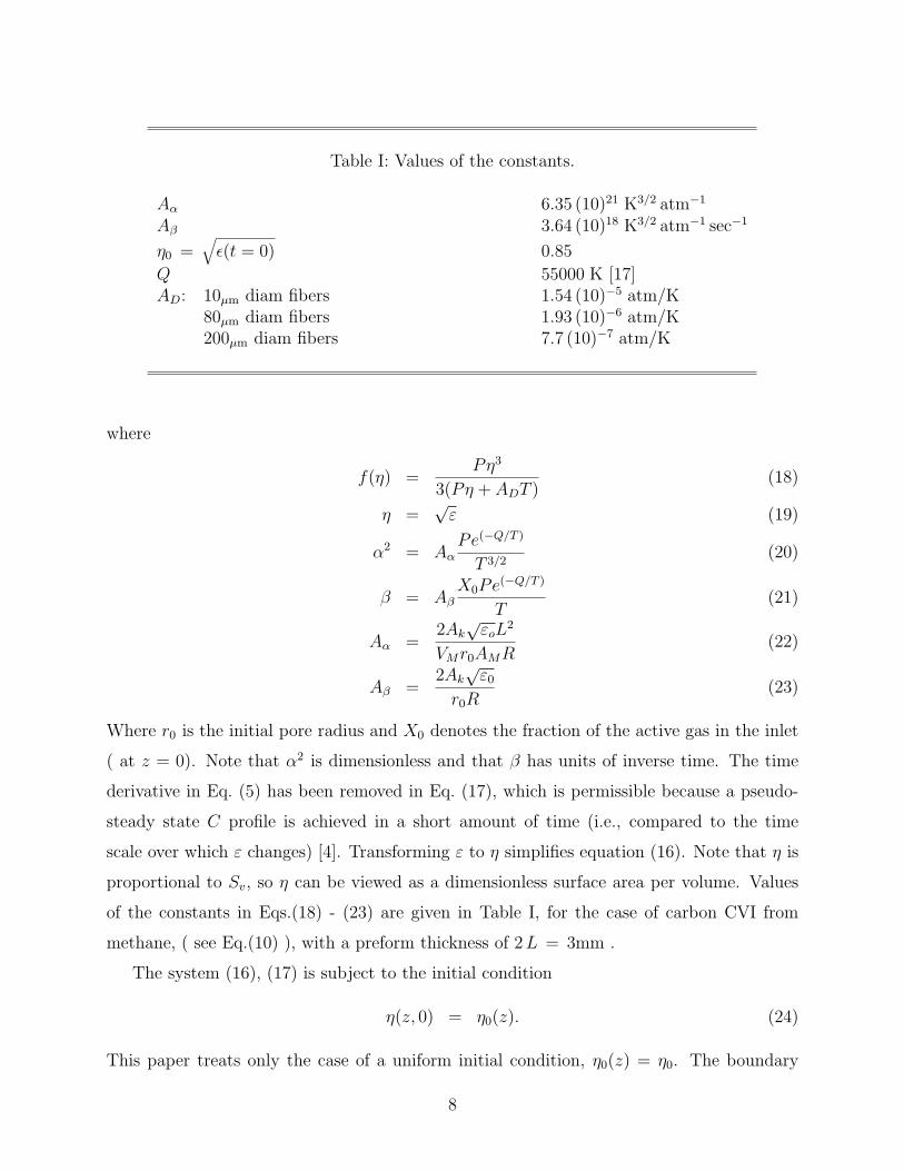
Table I: Values of the constants.

Aα 6.35 (10)21 K3/2 atm−1

Aβ 3.64 (10)18 K3/2 atm−1 sec−1

η0 =√

ε(t = 0) 0.85

Q 55000 K [17]AD: 10µm diam fibers 1.54 (10)−5 atm/K

80µm diam fibers 1.93 (10)−6 atm/K200µm diam fibers 7.7 (10)−7 atm/K

where

f(η) =Pη3

3(Pη + ADT )(18)

η =√

ε (19)

α2 = AαPe(−Q/T )

T 3/2(20)

β = AβX0Pe(−Q/T )

T(21)

Aα =2Ak

√εoL

2

VMr0AMR(22)

Aβ =2Ak

√ε0

r0R(23)

Where r0 is the initial pore radius and X0 denotes the fraction of the active gas in the inlet

( at z = 0). Note that α2 is dimensionless and that β has units of inverse time. The time

derivative in Eq. (5) has been removed in Eq. (17), which is permissible because a pseudo-

steady state C profile is achieved in a short amount of time (i.e., compared to the time

scale over which ε changes) [4]. Transforming ε to η simplifies equation (16). Note that η is

proportional to Sv, so η can be viewed as a dimensionless surface area per volume. Values

of the constants in Eqs.(18) - (23) are given in Table I, for the case of carbon CVI from

methane, ( see Eq.(10) ), with a preform thickness of 2 L = 3mm .

The system (16), (17) is subject to the initial condition

η(z, 0) = η0(z). (24)

This paper treats only the case of a uniform initial condition, η0(z) = η0. The boundary

8

conditions are (see (7), (8)):

c(0, t) = 1 (25)

∂c

∂z

∣∣∣∣∣z=1

= 0. (26)

With this model it can be shown that:

• The value of the void function in the inlet z = 0, is

η(0, t) = η0 − β

2t (27)

• There exists a critical time tc = 2η0

β. At this time, the void function vanishes at z = 0,

the inlet closes completely, and the process ends.

• The void function η and the concentration function c are bounded from above and

below. 0 < c(z, t) ≤ 1, η(0, t) ≤ η(z, t) ≤ η0 for t < tc = 2η0

β.

• For any time t < tc, the void function η(z, t) is monotonically increasing function of

the spatial variable z.

• The concentration function c(z, t) is monotonically decreasing function of the spatial

variable z.

The literature on diffusion and reaction in porous media typically uses a dimensionless

ratio of the diffusion and reaction rates, sometimes known as the Thiele modulus. This pa-

rameter varies during infiltration, because of changes in the microstructure with time. Thus,

previous CVI modeling has used an initial Thiele modulus as an approximate assessment of

the relative infiltration kinetics [4], [7], [8] , [10]. In terms of the formulation specified here,

the initial Thiele modulus is equal to α2η(z, 0)/f(η(z, 0)). In general, when α2 is small, dif-

fusion is fast and infiltration is relatively uniform. When α2 is large, the deposition reaction

is fast and infiltration is highly non-uniform.

The parameters α2 and β depend on the three key process variables: T , P , and X0.

Process optimization during CVI is achieved by setting these variables to optimal values. In

isothermal, isobaric CVI the infiltration kinetics are controlled by diffusion and the deposition

9

reaction. To achieve relatively uniform infiltration, diffusion must be fast relative to the

deposition rate. This is typically accomplished by choosing processing conditions that result

in a slow deposition rate, which usually leads to long infiltration times. Thus, the primary

basis for process optimization is to obtain the desired amount of infiltration in the shortest

possible time.

A general definition of a successful process includes two considerations:

1. At the end of the process ( at time t = tf ) the void function η(z, tf ) should be a small

fraction of its initial value, either in the whole interval or in a certain portion of the

interval 0 ≤ z ≤ z1.

2. For the process to yield good results it is important that the void function is uniformly

small along the z axis.

Mathematically, we express these considerations by stating that a process is successful if for

some time tf

η(z1, tf ) ≤ k1η0 (28)

η(0, tf ) = k0η0 (29)

k0 << 1, k0 < k1. Equation (28) states that the final values of the void function η should be

small in the interval between the inlet and the point z1 (note that η(z, t) is monotonically

increasing function of the spatial coordinate z). In most problems of interest z1 = 1. Condi-

tions (28) and (29) state that the void function should be uniformly small. Also, from (27),

(29), the final time, tf , is given by:

tf = (1− k0)η02

β. (30)

Note that the time for the process to end decreases as a function of β ( itself a function of

the temperature and pressure, given in (21) ).

The goal of the analysis in the following sections is to find the temperature and pressure

that minimize the final time tf for achieving a successful process.

10

III Analysis of the Optimization Problem

Evaluation of Eq.(27) requires an approximation for η(z1, tf ) in terms of the pressure

and temperature. There are two ways to obtain it: either by asymptotic expansions or by

direct numerical solution of the system (16),(17).

III.a Asymptotic Expansions

The set of equations (16), (17) is nonlinear and explicit solutions can not be obtained.

However some analytical approximation may be derived by noting that in most of the prob-

lems of interest α2 is small, and therefore it makes sense to expand the solutions in power

of α2. The details of obtaining this expansion to order α2 will be given elsewhere [16]. For

small α2 the final result is:

c(z, t) ∼ 1− α2(z − z2/2)f(E)

E(31)

η(z, t) ∼ E(t) + 3α2(z − z2/2)

[log

(η0

E(t)

)+

ADT

P

(1

E− 1

η0

)](32)

Where

E(t) = η0 − β

2t (33)

It can be shown that the error in the expansion is proportional to(

α2

k0

)2, where k0 is the

ratio between the final void function at the inlet and its initial value, as defined in (29). In

the next subsection the numerical results and the asymptotic expansions are compared, to

demonstrate the validity of the expansions in the range of relevant α2.

The asymptotic expansion (32) is used to get an explicit form for the uniformity constraint

(28) in terms of the temperature T and the pressure P . Substituting (32) into (28) gives:

k0η0 + 3α2(z1 − z21/2)

[log

(1

k0

)+

ADT

P η0

(1

k0

− 1)]

≤ k1η0 (34)

Substituting α2 from (20) and rearranging gives:

J(P, T ) ≤ (k1 − k0)η0. (35)

where

J(P, T ) = 3AαP

T 3/2e−Q/T (z1 − z2

1/2)

[log

(1

k0

)+

ADT

P η0

(1

k0

− 1)]

(36)

11

Rearranging terms shows that uniformity is assured if

P ≤ B0

B2

T 3/2eQ/T − B0

B2

T , (37)

where

B0 =η0(k1 − k0)

Aα3(z1 − z21/2)

(38)

B1 =AD

η0

(1

k0

− 1) (39)

B2 = log(1

k0

). (40)

These results can now be used to approximate the temperature and pressure that mini-

mize the infiltration time.Recall (see (30)) that the final time tf is inversely proportional to

β given in (21). The final time tf is therefore minimized if the function

F (P, T ) =P

Te−Q/T (41)

is maximized under the uniformity constraint (29). Inspection of (41) shows that in order

to maximize β we have to take the equality sign in (37). Substituting this into (41) , it is

easily verified that the following function must be maximized:

G(T ) =B0

B2

T 1/2 − B1

B2

e−Q/T (42)

This indicates that the final time tf to achieve a successful process is minimized by

choosing temperature and pressure satisfying

T 3/2eQ/T =B1Q

B0

(43)

P =B1

B2

(Q− T ) (44)

Moreover the minimal final time tminf is given by

tminf =

2(1− k0) log(1/k0)

k1 − k0

AαQ

AβX0

3(z1 − z21/2)

1

T 1/2(Q− T )(45)

Where the temperature T is given by (43).

2

12

The explicit formulas (43)-(45) lead to the following observations:

1. The minimum final time, tminf , decreases as AD decreases. (i.e. as the molecular

diffusion becomes dominant. )

2. tminf decreases as k1 increases. This reflects the fact that increasing k1 relaxes the

uniformity condition.

3. As z1 increases toward z1 = 1, the minimum final time tminf increases.

III.b Computational Results

In the previous subsection the asymptotic expansion of η was used to define a functional

J(P, T ) such that each pair P, T that satisfies J(P, T ) ≤ (k1−k0) η0 leads to a solution that

satisfies the conditions for a successful process, (28), (29). The optimal P and T was then

obtained based on the final time. This result is approximately correct since the asymptotic

expansion was used to approximate condition (28). This section uses numerical solutions of

(16),(17) to create a ’numerical J functional’, ( i.e. a functional relation between P and T

that ensures a successful process ).

Two algorithms were used to solve this problem: one based on a finite difference approx-

imation and one on spectral methods. These are described in the Appendix. The schemes

were run with k0 = 0.1, z1 = 1 and k1 = 0.15 or 0.7. Note that k1 = .15 corresponds to

relatively uniform infiltration while k1 = .7 is relatively non-uniform. Although most appli-

cations require relatively uniform infiltration (i.e., lower k1), there are some cases where a

non-uniform profile may be desirable. Two reasons for a higher k1 are that it enables faster

infiltration times, and it produces materials with lower density. For example, both of these

attributes are desirable during the formation of thin carbon-carbon composites for bipolar

plates in proton exchange membrane (PEM) fuel cells [18].

Three values were taken for AD, 1.54 (10)−5, 1.93 (10)−6 and 7.7 (10)−7 ( see Table I ).

Plots of the numerical and the asymptotic J curves are presented in Figure 1, plots of tf vs.

P are presented in Figure 2.

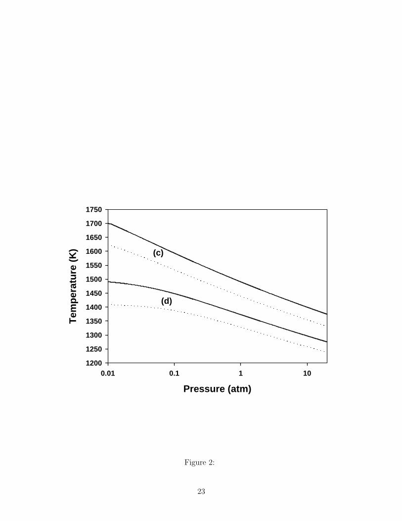
The process is very sensitive to changes in the temperature T, as can be seen, for example,

by comparing the results for P = .1atm,T = 1387 K, vs. P = .1atm, T = 1448 K ( for k1 = 0.7

and AD = 1.54 (10)−5 ) . Increasing temperature by 61 degrees, (∼ 4%), decreases the final

13

time from 160.3min to 31.4min, i.e. by a factor of 5 and produces an infiltration profile which

is much less uniform. This occurs because of the strong temperature dependence of the

deposition reaction. As the fibers size increases tf decreases slightly and the minimal time

occurs at lower pressures.

When the uniformity requirement dictates that k1 = .15 in (28), the condition J(P, T ) =

(k1−k0)η0 yields a P and T pair such that α2 ∼ .01. In this case, the asymptotic expansions

agree well with the numerical results. The predicted temperature that assures uniformity

differs by only few degrees from the one obtained numerically, and tf differs by less than

10%. When k1 was increased to 0.7, The large value of α2 , (∼ 0.1) leads to more inaccuracy

in tf , (See Table II ). However, the optimal temperatures predicted by the asymptotic result

is still accurate within10%.

Table II: tf for the optimal P and T .

Numerics AsymptoticsAD k1 P [atm] T [K] tf [H] P [atm] T [K] tf [H]

1.54 (10)−5 0.15 6.605 1201.65 16.03 7.694 1195.06 17.621.93 (10)−6 0.15 0.830 1258.48 15.27 0.962 1251.37 16.807.7 (10)−7 0.15 0.334 1389.75 14.93 0.373 1282.43 16.421.54 (10)−5 0.7 3.185 1338.99 0.3934 7.694 1265.75 1.4281.93 (10)−6 0.7 0.375 1492.76 0.3727 0.962 1405.28 1.3577.7 (10)−7 0.7 0.155 1573.00 0.3632 0.373 1478.51 1.324

In all cases, the asymptotic results agree qualitatively with the numerical results. The

curves obtained numerically were almost parallel to the asymptotic, and the points of minima

are almost in the same place. The asymptotic results are conservative, they always overesti-

mated the final time, and gave more restrictive conditions on P and T for uniformity. i.e. P

and T obtained by the asymptotic analysis never predict a successful process if it does not

exist. However, since P and T obtained by the asymptotic analysis may be much different

from the optimal ones ( obtained by the numerical analysis ), tf may be much larger then

the minimal value ( See Table II ).

14

IV Homogeneous Nucleation.

CVI processes can be limited by homogeneous nucleation (i.e., powder formation) in the

gas phase. This effect has not been treated in previous CVI models because it generally occurs

outside of the solid preform. However, powder formation can impose serious limitations on

CVI operating conditions during the formation of carbon and oxide matrices. Thus, this

phenomena imposes a constraint on the allowable CVI operating conditions. Nucleation

kinetics are typically described with:

I = ZIJ∗A∗(X0P/RT ) exp(−∆g∗/kBT ) (46)

where I is the steady-state nucleation rate, A∗ is the area of a critical cluster, J∗ is the

flux at which atoms are added to a critical cluster, ∆g∗ is the free energy barrier to forming

a critical cluster, kB is Boltzmann’s constant, and ZI is the so-called Zeldovich factor, see

[12]. A rigorous model requires that ZI be evaluated numerically, however, using standard

approximations for ZI , the pre-exponential terms in (46) can be combined to give:

I ∼= (X0P/RT )22(γ/kBT )1/2Ak exp(−Q/RT ) exp(−∆g∗/kT ) (47)

where γ is the surface free energy of the cluster, and the constants Ak and Q describe the

reaction rate constant (see (12) ). In practice, the permissible value of I depends on the

reactor configuration, as well as its actual value. For the current analysis, we assume that

powder formation limits CVI when the nucleation rate exceeds some allowable level, Ilim.

With this in mind, Eq. 46 can be revised to yield:

Alim = Ilimk1/2B /Akγ = (X0P )2/T 2.5 exp(−AI/T

m) (48)

where the two exponential terms in Eq. (47) have been combined to give one term with

two empirical constants, AI and m. Since ∆g∗ can have a relatively complex T dependence,

this empirical approach was adopted to provide a relatively simple expression. This form

was applied to the results of Loll et. al., who report threshold conditions for the onset of

significant nucleation (i.e., X0 vs. T at P = 1atm) [13], [14]. A good fit to their experimental

data was obtained with m = 1.5, AI = 750, 000 Km, and Alim = 3.3 (10)−17 atm2/K2.5. In

15

general, the value of Alim is somewhat arbitrary, since it reflects a threshold for a given reac-

tor. By varying Alim, it is possible to assess different tolerance levels for powder formation.

For example, recent carbon CVI experiments at Oak Ridge National Laboratory tolerate

higher powder formation levels than those described by Loll et.al. with a threshold value

that corresponds to Alim = 2.0 (10)−21 atm2/K2.5. [15].

The effect of adding the powder formation constraint can be seen from Figure 3, where

the I-curves are defined by Eq. (47). As seen in Figure 3a, the new constraint limits the

pressures and temperatures to values which are below both the I and the J-curves. For

a given pressure, the minimal tf corresponds to a temperature on either the I or J-curve

( whichever is lower ). Thus if the minimal tf found in section 3 ( i.e. when P and T are

on the J-curves ) to the left of the I-curve, then the additional constraint does not change

the previous results. If, on the other hand, this point is on the right of the I-curve then, the

minimal tf occurs at the intersection between the I and J-curves. This point can be clearly

seen as a cusp in the tf vs. P in the right plot.

A complete assessment of X0 effects requires solutions with the full Dusty Gas model,

because large values of X0 violate the assumption of a dilute reactant gas. However, con-

sidering only values up to X0 = 0.1 provides useful insight into optimizing dilute systems.

Without the homogeneous nucleation constraint (i.e., as Alim → ∞), the minimal time is

inversely proportional to X0, and the optimal pressure and temperature do not vary with X0

(see section 3). However, homogeneous nucleation limits the operating conditions when Alim

is low enough, as illustrated in Fig 3. The effect of this limitation on the optimal conditions

and on the minimal time are shown in Figs. 4 and 5. These results lead to the following

conclusions:

1. As in section 3, the asymptotic results are in good agreement with the numerical results

for k1 = .15, where α2 ∼ .01, and much less accurate in the case k1 = .7 where α2 ∼ .1.

In both cases, however, the asymptotic results agree qualitatively with the numerical

results.

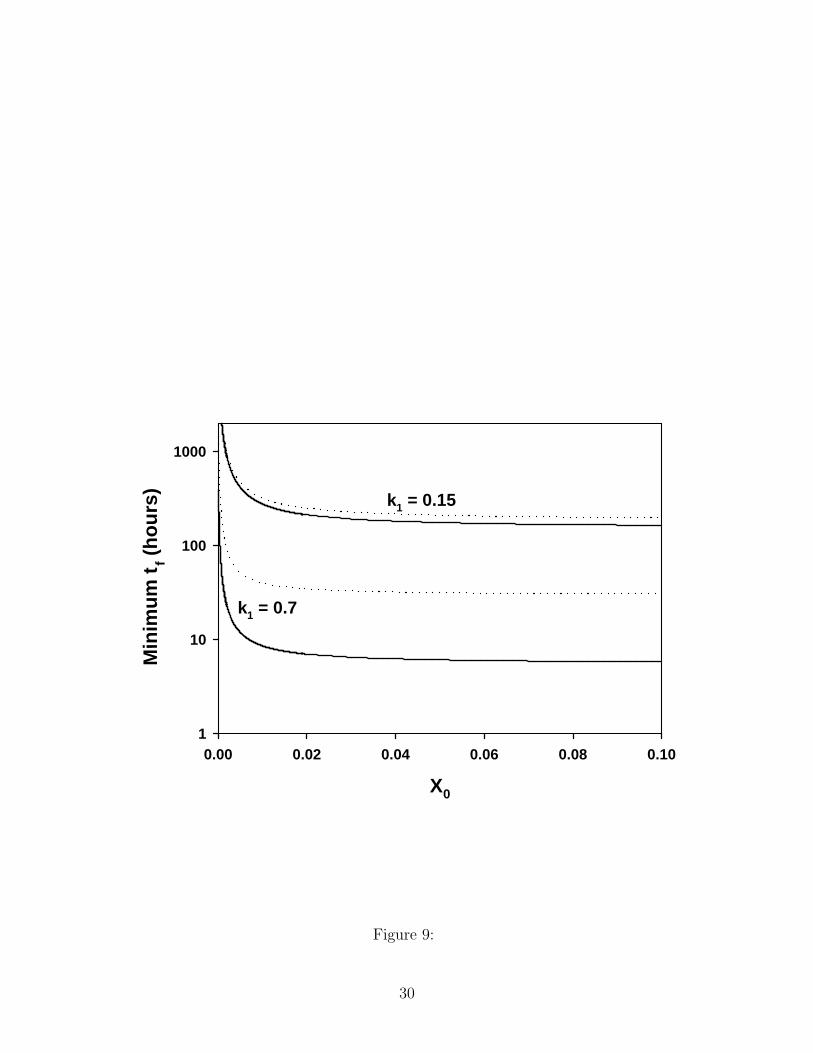
2. Notwithstanding the dilute reactant gas restriction, tf are monotonically decreasing

functions of X0, thus it is advisable to work in the ’highest’ X0 possible. However

since the optimal P is also a monotonically decreasing functions of X0, this value of

X0 is limited by the lowest operational pressure. For example for working pressure

16

of about 0.01atm, the maximum allowable X0 is only 0.05 , for 200µm diameter fibers

(AD = 7.7 (10)−7 atm K−1 ).

3. For a given X0, as the fiber diameter increases, P and tf decrease and T increases.

But unlike section 3, the differences here are significant. This occurs because the

homogeneous nucleation condition forces us to work in a region where the dependence

on AD is much stronger.

4. The homogeneous nucleation constraint causes the optimal temperature and pressure

to vary with X0.

As the value of Alim increases, the effects of homogeneous nucleation are less severe.

This can be seen in Fig. 6, which shows the effects of varying Ilim. Note that the minimum

infiltration time is dramatically increased when there is a significant limitation imposed by

homogeneous nucleation. In general, the process must be operated at lower pressures to avoid

powder formation. Some increase in the corresponding optimal temperature accompanies this

decrease in pressure. The slope discontinuities in Fig. 6 correspond to the conditions where

the homogeneous nucleation constraint no longer has an effect, ( i.e. the optimal conditions

are determined solely by the J curve ).

V Conclusions

Minimizing infiltration times for isothermal, isobaric CVI is important because process-

ing times are typically very long. The work presented here provides a detailed assessment

of the pressure and temperature which will minimize the total required time, based on a

simplified model for a single, dilute reactant species. This formulation makes it possible

to understand the basic physics of the problem in terms of a relatively small number of

lumped parameters. The basic objective of this optimization problem is to obtain a den-

sity profile with a prescribed amount of uniformity, in the shortest possible time (section

3). The asymptotic results are particularly useful, because they make it possible to deter-

mine optimal conditions without doing numerical calculations (under conditions where α2

is small enough). Based on comparisons with the numerical results, the asymptotic forms

are also qualitatively accurate when α2 is larger. Thus, the asymptotic results provide a

17

clear understanding of how the optimal conditions are related to the key parameters for the

problem.

The effects of homogeneous nucleation were also analyzed, as an additional constraint

on the basic optimization problem. This issue has not been considered in previous work on

CVI modeling, however, it can limit operating conditions in systems were powder formation

is significant (e.g., the formation of carbon matrix composites). The results obtained here

provide a quantitative assessment of the conditions where homogeneous nucleation imposes

limitations on infiltration conditions. When these limitations occur, powder formation also

increases the minimum infiltration time.

VI Appendix

To gain confidence in our computations, two completely different numerical methods

were used: the pseudospectral method and a finite difference method.

• In the pseudospectral Chebyshev method the grid points is chosen to be

zj =1 + cos(πj

N)

20 ≤ j ≤ N (49)

where N is the total number of grid points and was 10 for most of the runnings.

The spectral differentiation matrix takes the value of a given function at the g rid

points zj and yields the values of the derivative of the interpolation polynomial at

these poi nts. The points zj are the nodes of the Gauss Lobatto Chebyshev quadrature

formula. The matrix can be writt en explicitly:

Djk = 12

cj

ck

(−1)j+k

sin π2N

(j+k) sin π2N

(−j+k)j 6= k ,

Djj = −12

zj

sin2( πN

j)j 6= 0, N ,

D00 = −DNN = 2N2+16

(50)

We apply the matrix Djk twice, once for the vector c taking into account the boundary

condition c(0, t) = 1 and then to f(η) cz and taking into account that cz(1, t) = 0. This

yields a linear system for the values of c(zj, t).

In the next stage we update η by the standard third order Runge-Kutta sch eme.

18

• A second-order finite-difference scheme using the equidistance grid

zj =j

N= j h 0 ≤ j ≤ N . (51)

The differentiation matrix can be written explicitly:

D1 1 = − 1h2 (f(z1 − h/2) + f(z1 + h/2))

D1 2 = 1h2 f(z1 + h/2)

j = 1Dj j−1 = 1

h2 f(zj − h/2)Dj j = − 1

h2 (f(zj − h/2) + f(zjh/2))Dj j+1 = 1

h2 f(zj + h/2)j = 2 . . . N − 1

DN N−1 = 2h2 f(1− h/2)

DN N = − 2h2 (f(1− h/2) + α2 η)

f in the mid-points was interpolated. In each step we Solve the system

D c =

− 1h2 f(z1 − h/2)

0...0

,

In the next stage we use c to update η by the standard fourth order Runge-Kutta

scheme. Since this scheme is less accurate we used 80 grid points.

The results of both schemes were compared and the differences in η(z, tf ) were less then

10−6.

References

[1] E. Fitzer and R. Gadow, Am Ceram. Soc. Bull, 65, 326-55 (1986).

[2] S.M. Gupte and J.A. Tsamopoulos, J. Electrochem. Soc., 136, 555-61 (1989).

1104-9 (1991).

[3] Aris, R., The Mathematical Theory of the Diffusion and Reaction in Permeable Cata-

lysts, Oxford University Press, London, 1975.

[4] H.-C. Chang, Minimizing Infiltration Time during Isothermal Chemical Vapor Infiltra-

tion, Ph. D. Thesis, Brown University, 1995.

19

[5] Dullien, F. A. L., Porous Media: Fluid Transport and Pore Structure, Academic Press,

New York, 1979.

[6] Mason, E. A. and A. P. Malinauskas, Gas Transport in Porous Media: The Dusty-Gas

Model, Elsevier Science Publisher, 1983.

[7] B.W. Sheldon and H.-C. Chang in Ceramic Transactions, Vol. 42, editedby B.W.

Sheldon and S.C. Danforth (American Ceramic Society, 1994), pp. 81-93.

[8] H.-C. Chang, T.F. Morse, and B.W. Sheldon, J. Mater. Proc. Manuf. Sci. 2, pp. 437-

454 (1994).

[9] J.Y. Ofori and S.V. Sotirchos, AIChE Journal, 42, pp. 2828 (1996).

[10] H.-C. Chang, T.F. Morse, and B.W. Sheldon, J. Am. Ceram. Soc., 7, pp. 1805-11

(1997).

[11] H.-C. Chang, D. Gottlieb, M. Marion, and B.W. Sheldon, J. of Scientific Computing,

13, pp. 303-21 (1998).

[12] J. Feder, K.C. Russell, J. Lothe, and G.M. Pound, Adv. Phys., 15, 111 (1966).

[13] P. Loll, P. Delhaes, A. Pacault, and A. Pierre, Carbon, 13, 159 (1975).

[14] P. Delhaes in Electrochemical Society Proceedings 97-25, edited by M.D. Allendorf and

C. Bernard (Electrochemical Society, 1997), pp. 486-95.

[15] T.M. Besmann, Oak Ridge National Laboratory, unpublished results (1998).

[16] A. Ditkowski, D. Gottlieb and and B.W. Sheldon, On the Mathematical Analysis

and Optimization of Chemical Vapor Infiltration in Materials Science, M2AN, 34(2),

337-351 (2000).

[17] S. Bammidipati, G.D. Stewart, G.R. Elliott,Jr., S.A. Gokoglu, M.J. Purdy. , AIChE

Journal, 42, No.11, pp. 3123-3132 (1996).

[18] T.M. Besmann, J.W. Klett, and T.D. Burchell, in MRS Symposium Proceedings, pp.

365-370 (Materials Research Society, Pittsburgh, 1998).

20

Figure Captions:

Figure 1. J Curves obtained both numerically (solid lines) and by asymptotic analysis

(dotted lines). Conditions on or below these lines will satisfy the uniformity condition (Eq.

(3.35)). Conditions above this line do not satisfy the uniformity condition. All cases here

correspond to X0 = 0.1, with: (a) k1 = 0.15, 10µm diameter fibers; (b) k1 = 0.15, 200µm

diameter fibers; (c) k1 = 0.7, 10µm diameter fibers; (d) k1 = 0.7, 200µm diameter fibers.

Figure 2. Times which correspond to conditions on the J curves in Fig. 1, with values

obtained both numerically (solid lines) and by asymptotic analysis (dotted lines). The filled

circles show the minimal time. (a) k1 = 0.15, 10µm diameter fibers; (b) k1 = 0.15, 200µm

diameter fibers; (c) k1 = 0.7, 10µm diameter fibers; (d) k1 = 0.7, 200µm diameter fibers.

Figure 3. Effect of homogeneous nucleation for k1 = 0.7, X0 = 0.01, 10µm diameter

fibers. (a) The numerically obtained J Curve (uniformity constraint, Eq. (35)) and the I

Curve (nucleation limit, Eq. (48) with Alim = 2.0 (10)21). (b) Limiting time as a function

of pressure. The left part of the curve is determined by the numerically obtained J Curve

and the right side is determined by the I Curve, with the minimal time shown by the filled

circle. The dotted line corresponds to the approximate J Curve which was determined with

asymptotics.

Figure 4. Effect of X0 with 10µm diameter fibers: (a) optimal pressures; (b) optimal

temperatures; (c) minimum infiltration times.

Figure 5. Effect of X0 with 200µm diameter fibers: (a) optimal pressures; (b) optimal

temperatures; (c) minimum infiltration times.

Figure 6. Effect of Alim on tf , with k1 = 0.15: (a) 10µm diameter fibers and X0 = 0.1;

(b) 10µm diameter fibers with X0 = 0.02; (c) 10µm diameter fibers with X0 = 0.1. All

values are based on numerical results.

Figure 7. Effect of Alim on the optimal pressure, for the same cases plotted in Fig. 6.

Figure 8. Effect of Alim on the optimal temperature, for the same cases plotted in Fig.

6.

21

Pressure (atm)

0.01 0.1 1 10

Tem

per

atu

re (

K)

1150

1200

1250

1300

1350

1400

1450

1500

1550

(a)

(b)

Figure 1:

22

Pressure (atm)

0.01 0.1 1 10

Tem

per

atu

re (

K)

1200

1250

1300

1350

1400

1450

1500

1550

1600

1650

1700

1750

(c)

(d)

Figure 2:

23

Pressure (atm)

0.01 0.1 1 10

t F (

ho

urs

)

10

20

40

60

80

100

150

200

(a)

(b)

Figure 3:

24

Pressure (atm)

0.01 0.1 1 10

t F (

ho

urs

)

0.3

1

3

10

30

(c)

(d)

(d)

(c)

Figure 4:

25

Figure 5:

26

Figure 6:

27

X 0

0.00 0.02 0.04 0.06 0.08 0.10

Op

tim

al P

ress

ure

(at

m)

0.001

0.01

0.1

1

k 1 = 0.7

k 1 = 0.15

Figure 7:

28

X 0

0.00 0.02 0.04 0.06 0.08 0.10

Op

tim

al T

emp

erat

ure

(K

)

1200

1250

1300

1350

1400

1450

1500

k 1 = 0.7

k 1 = 0.15

Figure 8:

29

X 0

0.00 0.02 0.04 0.06 0.08 0.10

Min

imu

m t

f (h

ou

rs)

1

10

100

1000

k 1 = 0.7

k 1 = 0.15

Figure 9:

30

X 0

0.00 0.02 0.04 0.06 0.08 0.10

Op

tim

al P

ress

ure

(at

m)

0.001

0.01

0.1

k 1 = 0.7

k 1 = 0.15

Figure 10:

31

X 0

0.00 0.02 0.04 0.06 0.08 0.10

Op

tim

al T

emp

erat

ure

(K

)

1300

1350

1400

1450

1500

1550

1600

1650

1700

1750

1800

k 1 = 0.7

k 1 = 0.15

Figure 11:

32

X 0

0.00 0.02 0.04 0.06 0.08 0.10

Min

imu

m t

f (h

ou

rs)

1

10

100

k 1 = 0.7

k 1 = 0.15

Figure 12:

33

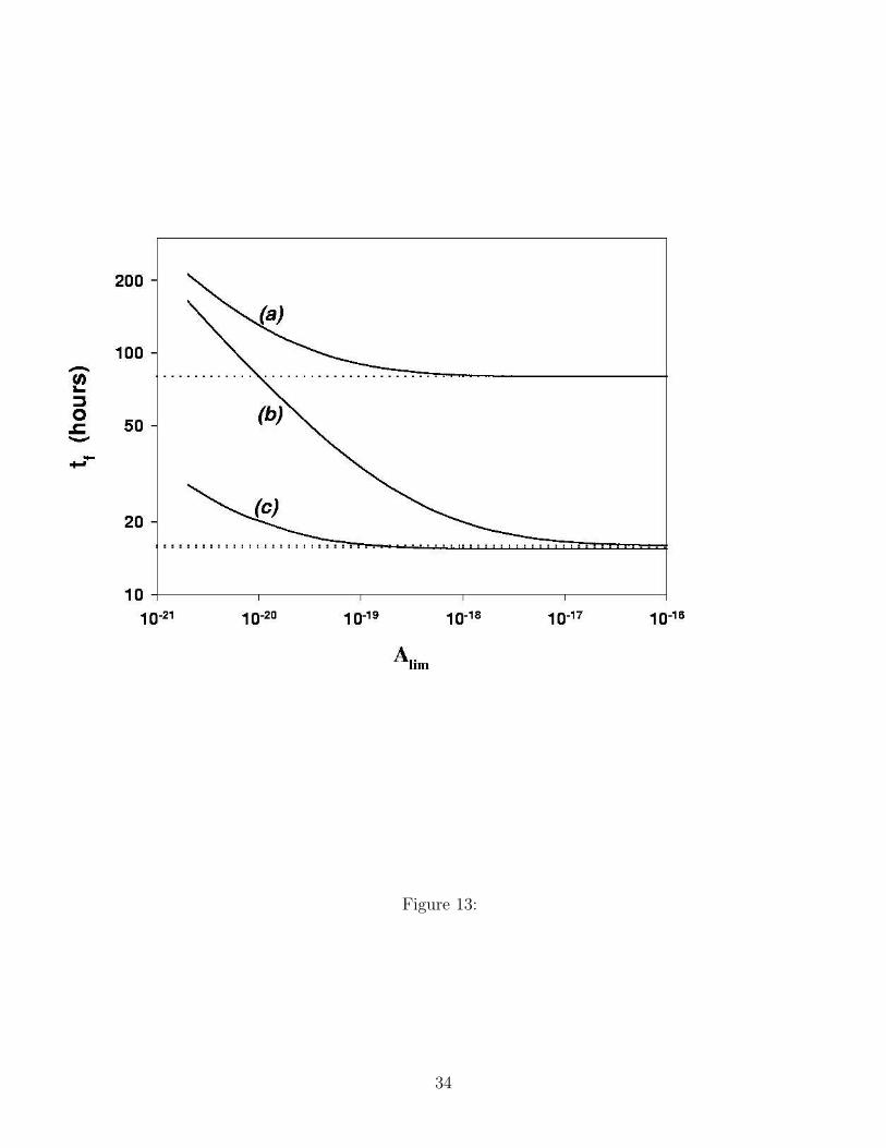
Figure 13:

34

Figure 14:

35

Figure 15:

36