
Optimise initial spare parts inventories: an analysis and ...core.ac.uk/download/pdf/6499176.pdf ·...
79
Optimise initial spare parts inventories: an analysis and improvement of an electronic decision tool M.E. Trimp, BSc, S.M. Sinnema, BSc, Prof. dr. ir. R. Dekker* and Dr. R.H. Teunter Department of Econometrics and Management Science, Erasmus University Rotterdam, P.O. Box 1738, 3000 DR Rotterdam, The Netherlands Report Econometric Institute EI 2004-52 Abstract Control of spare parts is very difficult as demands can be very low (once in a few years is no exception), while the consequences of a stockout can be severe. While in the past many companies choose to have very large spares inventories, one now observe trends in areas with good transportation connections to keep spare parts at the suppliers. Hence it is very important to make a good selection of which spare parts to stock at the start-up of new plants. To this end Shell Global Solutions has developed an electronic decision tool, called E-SPIR. In this report we analyse the decision rules used in it. We consider stockout penalties and advise to use criticality classifications instead. Furthermore, we investigate minimum stock levels, demand distributions and order quantities. * Corresponding author: E-mail: [email protected]
Transcript of Optimise initial spare parts inventories: an analysis and ...core.ac.uk/download/pdf/6499176.pdf ·...
Optimise initial spare parts inventories:
an analysis and improvement of an
electronic decision tool
M.E. Trimp, BSc, S.M. Sinnema, BSc, Prof. dr. ir. R. Dekker* and Dr. R.H. Teunter
Department of Econometrics and Management Science, Erasmus University
Rotterdam, P.O. Box 1738, 3000 DR Rotterdam, The Netherlands
Report Econometric Institute EI 2004-52
Abstract
Control of spare parts is very difficult as demands can be very low (once in a few years is no exception), while the consequences of a stockout can be severe. While in the past many companies choose to have very large spares inventories, one now observe trends in areas with good transportation connections to keep spare parts at the suppliers. Hence it is very important to make a good selection of which spare parts to stock at the start-up of new plants. To this end Shell Global Solutions has developed an electronic decision tool, called E-SPIR. In this report we analyse the decision rules used in it. We consider stockout penalties and advise to use criticality classifications instead. Furthermore, we investigate minimum stock levels, demand distributions and order quantities. * Corresponding author: E-mail: [email protected]

Report December 2004 – Erasmus University Rotterdam
1
Index
Summary...................................................................................................... 4
1. Motivation and background .................................................................... 8
1.1 Introduction ...........................................................................................8 1.2 Purpose of this research ..........................................................................8 1.3 E-SPIR program......................................................................................9 1.4 Problem formulation ...............................................................................9 1.5 Input data E-SPIR.................................................................................10 1.6 Requirements of the program................................................................11 1.7 Literature overview...............................................................................11 1.8 Overview of this report .........................................................................12
2. Information needed ..............................................................................13
2.1 Introduction .........................................................................................13 2.2 Parameters for the whole project...........................................................13
2.2.1 Introduction ...................................................................................13 2.2.2 Percentage to increase prices..........................................................13 2.2.3 Values to adjust (increase) lead times .............................................14 2.2.4 Order cost......................................................................................14 2.2.5 Holding cost rate ............................................................................15 2.2.6 Minimum Period to cover ................................................................15 2.2.7 Maximum Period to cover................................................................15
2.3 Parameters for the equipment...............................................................16 2.4 Parameters for the parts.......................................................................16
2.4.1 Introduction ...................................................................................16 2.4.2 Price ..............................................................................................16 2.4.3 Lead time.......................................................................................16 2.4.4 Consumption rate...........................................................................17
2.5 Penalty Values......................................................................................18 2.6 Conclusion............................................................................................19
3. Holding Cost Rate..................................................................................20
3.1 Introduction .........................................................................................20 3.2 Theory .................................................................................................20 3.3 Stocking costs in an Oil Company..........................................................21 3.4 New items on stock ..............................................................................22 3.5 Classifications and volume ....................................................................23 3.6 Conclusions..........................................................................................23
4. To stock or not to stock ........................................................................25
4.1 Introduction .........................................................................................25 4.2 Variables..............................................................................................25 4.3 Stocking decision rule ...........................................................................26 4.4 Auxiliary (Low) one-time costs ..............................................................28 4.5 Conclusion............................................................................................31
Report December 2004 – Erasmus University Rotterdam
2
5. Economic Order Quantity ......................................................................32
5.1 Introduction .........................................................................................32 5.2 Theory .................................................................................................32 5.3 EOQ: theory and formula ......................................................................33 5.4 Input variables .....................................................................................34 5.5 Rounding..............................................................................................35 5.6 Examples.............................................................................................35 5.7 Dealing with maximum period to cover..................................................36 5.8 Conclusion............................................................................................37
6. Minimum Stock......................................................................................38
6.1 Introduction .........................................................................................38 6.2 Determining the Minimum Stock............................................................38 6.3 Distribution of the consumption .............................................................40
6.3.1 Introduction ...................................................................................40 6.3.2 Number of items replaced at once ...................................................41 6.3.3 Factor Variance Method ..................................................................41 6.3.4 Erlang-k Method.............................................................................43 6.3.5 Simple Minimum Stock Method........................................................47 6.3.6 Conclusion .....................................................................................47
6.4 Total Costs Minimum Stock ...................................................................48 6.4.1 Introduction ...................................................................................48 6.4.2 Holding costs..................................................................................48 6.4.3 Penalty costs..................................................................................50
6.5 Advise..................................................................................................51 6.6 Maximum stock ....................................................................................52 6.7 Conclusion............................................................................................52
7. Penalty Values.......................................................................................53
7.1 Introduction .........................................................................................53 7.2 Penalty values and Service levels ..........................................................53 7.3 Example...............................................................................................54 7.4 Argumentation .....................................................................................55 7.5 Conclusion............................................................................................56
8. Sensitivity analysis ...............................................................................57
8.1 Introduction .........................................................................................57 8.2 Sensitivity analysis EOQ........................................................................57 8.3 Holding Cost Rate .................................................................................60 8.4 Conclusion............................................................................................62
9. Conclusions and recommendations......................................................63
References .................................................................................................66
Report December 2004 – Erasmus University Rotterdam
3
Appendix 1. Formulas for the indices of the stocking decision rule .......68
Appendix 2.A. Index values for the decision rule (Vital and Essential) .69
Appendix 2.B. Index values for the decision rule (Auxiliary).................70
Appendix 3. Minimum Stock Computations..............................................71
A Probability of Stock out for the Minimum Factor Method ............................71 B Probability of Stock Out for the Erlang-k Method.......................................73 C Penalty Costs for the two methods...........................................................74
Appendix 4. Percentage Cost Penalty .......................................................78

Report December 2004 – Erasmus University Rotterdam
4
Summary
Spare part inventories can be very high when poor inventory systems are used.
On the other hand the costs associated to not having a spare part when needed
can be significant. A good balance between holding costs associated to having
parts and penalty costs associated to stockouts is therefore needed. This balance
is especially important for slow moving items. Inventory systems often contain
methodologies to achieve the optimum inventory cost based on historical
consumption information. For projects aiming at the construction of new plants
this information is not available. A software tool called E-SPIR has been
developed by Shell Global Solutions to collect the spare parts information in a
standard format and facilitate the review and ordering of the spare parts.
E-SPIR stands for Electronic – Spare Parts and Interchangeability Record, which
is the electronic version of the SPIR. In this report the spare parts selection
procedure present in the E-SPIR is analysed and improved. This is achieved by
addressing the following four main questions.
1. To stock or not to stock an item?
In general, items should only be stocked if the benefits of direct availability
outweigh the costs of holding the items in stock. The decision to stock is
especially important for slow moving parts as wrong decisions have very long-
lasting effects. A comparison of costs associated with stocking one spare part
and those associated to not stocking at all will give an answer on to stock or not.
An easy to follow rule was developed by Olthof and Dekker (1994). This decision
rule is based on four variables: consumption rate, price, leadtime and penalty
costs. The first three variables should be given by the supplier of the item, the
last by the user/company. The first parameter is difficult to estimate by either
supplier or user/Company, yet an estimate can be given. The fourth variable,
penalty costs, is also difficult to estimate. In the old version of the E-SPIR the
user/company has to give an explicit value for these costs. In practice this
appeared to be too difficult as the engineers involved have little insight into cost
consequences. In the new version of the E -SPIR an item belongs to one of three
criticality classifications: Vital (High), Essential (Medium) or Auxiliary (Low). To
each of these classes a range of penalty costs is associated. Now the
user/company only has to choose a range for each criticality classification once,

Report December 2004 – Erasmus University Rotterdam
5
at the start of a new plant, and subsequently has to give each item a criticality
classification . In the current situation the penalty costs for all the criticality
classifications are values per day. In practice it is found that for the classification
Auxiliary (Low) a one-time penalty cost will be sufficient. An extra possibility is
given to take o f a period before which costs are incurred (so -called zero-cost
days) for the classifications Vital (High) and Essential (Medium). This is done on
project level and thus needs to be given by the user/company once, at the start
of a project.
2. How many to order at once?
When the decision has been made to stock an item, the next question to answer
is how many to order at once. At the start of a new plant, this is the initial
purchase order. To determine an optimal order quantity, a well-known result in
the inventory control area is used, viz. the classical economic order quantity
(EOQ) formula. The EOQ is essentially an accounting formula that determines the
inventory level at which the combination of order costs and holding costs are the
least. The input variables needed are the annual consumption, the order costs
and the holding costs. Not all assumptions of the EOQ hold in the case of slow
moving items. Because an integer number is needed, the EOQ is rounded off.
When an item needs to be stocked, at least one item is ordered. Further it is
shown that the normal rounding rules can be applied.
3. When to release a new order?
The moment to release a new order is usually named the re -order point. The
minimum stock is the level of inventory on stock before a replenishment order is
placed (this is the re-order point plus one). Additional costs associated with a
wrong decision on the minimum stock can be high. Having too many items on
stock can result in high holding costs. On the other hand, having too few items
on stock can result in high penalty costs. The minimum stock will be determined
considering the consumption during the lead time. This consumption gives the
estimated number of items needed during the lead time of the ordered items.
The consumption during the lead time depends on the distribution of this
consumption. Three different methods are investigated. First the what we call
Factor Variance Method. In this method the consumption during the leadtime is
considered to be normally distributed. Here the minimum stock consists of the

Report December 2004 – Erasmus University Rotterdam
6
mean demand during the leadtime plus a safety factor times the standard
deviation of the demand during the lead time. For different levels of minimum
stock the total costs (holding costs + penalty costs) are considered and the level
with the lowest costs is chosen. For slow moving items the normal distribution is
not very suitable, because of a significant probability of negative demand (which
is impossible in reality, of course). The second method is based on the
assumption that the time between two successive demands follows an Erlang-k
distribution. The larger the shape parameter k, the less variance such a
distribution will have. Given the value for k, the yearly consumption and the lead
time, the probability of a stock out can be computed for different levels of
minimum stock. Again the level with the lowest total costs is chosen. The third
method is a very simple estimation of the number of needed items during a
period. This method is not a scientific method but it is often used as a “common
sense” idea. The idea of the method is to increase the lead time with a safety
factor to reach a higher level of minimum stock. A main disadvantage of this
approach is that it does not take holding costs and penalty costs into account.
The conclusion is that the best method for slow moving spare parts is the Erlang-
k method. Although a choice for the appropriate k is difficult, we advise to use
k=4 in case parts are installed in one or two pieces of equipment only and the
plant can be re -supplied in a quick way. In all other cases we advise to be on the
safe side and use a value of k=1.
4. How to cope with penalty values?
The minimum stock discussed above is based on costs. Penalty costs express the
importance of having an item on stock. Another method to express this
importance is the use of service levels. In the service sector service levels are
often used. It is a relatively easy way to express the risk one is willing to take. In
a call centre for example one can require that 99 of 100 people will not get a
busy line. We will discuss the pros and cons of working with service levels and
with stockout costs. When these costs are known, they can be used to balance
the expected total costs. For the criticality classification Vital (High) and Essential
(Medium) these costs are expressed in days. For the third criticality classification
Auxiliary (Low) these are one time penalty costs. On a project level, each of
these classifications needs to be given a pre -defined range of costs.
Report December 2004 – Erasmus University Rotterdam
7
Besides these four main questions the input variables needed for the inventory
system are discussed in detail. It is very important to know exactly what each
variable means and how to determine its value. For the holding costs, a holding
cost rate is used. This rate is multiplied by the purchase costs to compute the
holding costs. Because this rate is difficult to determine, a separate chapter is
devoted to it. In a sensitivity analysis it is concluded that the economic order
quantity and the holding cost rate are quite robust to this cost rate.
Report December 2004 – Erasmus University Rotterdam
8
1. Motivation and background
1.1 Introduction
Developments of modern information technology open up new possibilities for a
more efficient control of inventory systems. Most organizations can reduce their
costs substantially with this knowledge. In this research the initial spare part
inventory procedures of a group of companies in the oil and gas sector a re
analysed. In this chapter the motivation and background of this research is
presented. In section 1.2 the purpose of this research is explained. Next some
information is given about the E -SPIR program (section 1.3). In section 1.4 the
problems addressed in this research are formulated. Subsequently the input
variables needed in the program are summed up (section 1.5). In section 1.6 the
requirements of the program are shortly stated. This chapter ends with a preview
of the following chapters (section 1.7).
1.2 Purpose of this research
This research was motivated by Shell Global Solutions International to improve
the inventory model of spare parts. For collecting the spare parts information in a
standard format they use the E -SPIR program. One of the strengths of th is
program is the facility to advise the inventory level at the start of a plant. Slow
moving items are the most crucial in this respect. These are items with a
consumption of at most 2 items per year. When an error is made in the minimum
stock, these items stay on stock for a long time. Costs of stocking items too long
can be high (e.g. due to obsolescence ). The difficulty faced however, at the
moment of the start of plant is the lack of historical information, on which the
decision can be based of how many to stock.
The reason for having initial spare part inventories is to immediately provide
parts when needed due to failures. It is essential that the chance of a part being
out of stock when required is kept low. However, because inventory is expensive
and can become obsolete as equipment models change, companies do not want

Report December 2004 – Erasmus University Rotterdam
9
to hold excessive amounts of stock. Therefore, understanding the inventory
versus costs due to failures and striking a reasonable balance are a firm’s
primary concern and the main motivation for this research. The purpose of this
research is to make improvements to the present initial spares selection
procedure.
1.3 E-SPIR program
E-SPIR stands for Electronic – Spare Parts and Interchangeability Record, which
is the electronic version of the SPIR, see e.g. http://www.e-spir.com . The
program shows the relation between Equipment and Spare parts and the
interchangeability between Spare parts in equipment installed. This program was
developed by Shell Global Solutions International to assist in reviewing and
selecting spare parts for new installations. The program makes use of data
submitted by suppliers, completed with available information from the
project/company. In this research the spare selection procedure present in the E-
SPIR will be analysed and improved. Additional information required from the
user/company should be minimal to keep the program user-friendly.
1.4 Problem formulation
Four separate questions will be addressed in this research:
1. To stock or not to stock an item?
2. How many to order at once?
3. When to release a new order?
4. How to cope with penalty values?
In the E-SPIR program a stock recommendation gives project users advise
whether to stock or not to stock the spare part. This rule was developed by
Olthof and Dekker (1994). In this research some adjustments to this rule are
studied. When the decision to stock an item has been made, the next question is
how many and when to order. The number to order at a time is currently based

Report December 2004 – Erasmus University Rotterdam 10
on an estimated quantity to cover the delivery time of the relevant spare part.
Costs were not included in the present estimate in the E-SPIR. In this report a
scientific basis for an economic order quantity (EOQ) in the E -SPIR program is
provided. To answer the question when to order, different demand distributions
are discussed to determine the minimum stock level. The fourth question is of a
different kind, but in this research at least as important. Penalty values are
important throughout the report. It is important to know how to determine the
penalty values and what this means for the stocking decision and for the
minimum stock. Also the difference between using penalty values and service
levels is discussed.
1.5 Input data E-SPIR
The input data of the E -SPIR program is split over three levels. These levels are
project, equipment and parts. A project is for example the construction of a gas
plant, a whole or part of a refinery or an oil platform. Each project involves a
large amount of equipment and per equipment many parts are involved, usually
more than 1000 different pieces. The three different levels are introduced
because of the different information needed per level. Some information can be
asked once and used throughout the entire project. For each level we give below
a summary of the data needed to answer the main four inventory questions (see
section 1.4). In chapter 2 these variables are explained in more detail.
Project/Company:
Ø A price surcharge (in percentages) for all parts (e.g. for handling and
import duties)
Ø A lead time surcharge because of the ordering, transport and handling
time of the plant (in weeks)
Ø Average costs to place one order
Ø Holding Cost Rate
Ø Minimum period to cover
Ø Maximum period to cover
Ø Penalty values and zero -cost-days for the different criticalities of
equipment

Report December 2004 – Erasmus University Rotterdam 11
Equipment
Ø Criticality classification
Parts:
Ø Price of the item
Ø Lead time (days) required to replenish inventory
Ø Estimated consumption rate (items a year)
1.6 Requirements of the program
Any changes to the existing program as well as the additional information
needed from the user/ company should be easy to implement, in the sense that
a. The stock quantity decision process does not depend on difficult-to-
estimate parameters.
b. The policies lead to closed-form expressions for stocking parameters
that can be computed with minimal user input in a spreadsheet.
c. The program provides a minimum and maximum stock
recommendation.
The challenge is to make appropriate use of available data with minimal manual
interaction allowing stocking policies to be easily and effectively implemented for
the spare parts selection and ordering process in projects.
1.7 Literature overview
A review of the scientific literature (see Kennedy et al. (2002) reveals that the E-
SPIR program is unique in its kind. There are several programs (e.g. Sparecalc, a
program from Shell Expro, Relex OpSim software optimising spare parts), that
can calculate the right number of a certain kind of spare. However, they usually
ask a lot of questions and take relatively much time to give an advise. They
should primarily be used for the very expensive (price > 10,000 USD) spares.
Accordingly, they can not be used to scan the multitude of spares which are
advised by a supplier in a large project. There are yardsticks based on a VED
Report December 2004 – Erasmus University Rotterdam 12
(Vital, Essential and Desirable) analysis (see e.g. Mukhopadhyay (2003)), but
they are very superficial and the coding directly implies the stocking decision
(see e.g. Botter and Fortuin (2000)). There is a Spares calculater (see Mickel and
Heim (1990)), but that is a manual instrument only. Already in the research of
Olthof and Dekker (1994) it became clear that easy data entry and handling,
easy and quick parameter estimation, fast computation and finally a good coding
of the parts, are the crucial aspects in assessing stocking decisions for many
spare parts. The present E-SPIR program is especially developed for this
purpose.
1.8 Overview of this report
This report is divided in nine chapters. After this introduction on the research the
different input variables are discussed in chapter 2. Chapter 3 explains one of the
variables in more detail, namely the holding cost rate. The first question, to stock
or not to stock an item, is addressed in chapter 4. The old decision rule is
discussed and changes are suggested. In chapter 5 the second question of how
much to order is investigated. The Economic Order Quantity (EOQ) will be
introduced. The third question of when to re -order is reviewed in chapter 6.
Different demand probabilities are suggested to compute a minimal stock. The
reorder point is the moment when the inventory level falls down this minimum
stock. In chapter 7 the penalty values are discussed, also in respect with service
levels. Because different methods are discussed and used, a sensitivity analysis
is given in chapter 8. This analysis is done for the Economic Order Quantity
(EOQ) and the Holding Cost Rate. Finally, in chapter 9 conclusions and
recommendations will be given.

Report December 2004 – Erasmus University Rotterdam 13
2. Information needed
2.1 Introduction
In this chapter all the inputs are discussed, which are needed for giving a
stocking advise for a large capital project. First the parameters for the whole
project are explained in section 2.2, thereafter (section 2.3) the parameters for
the equipment are discussed. In section 2.4 the parameters for the individual
parts are explained. The penalty costs need to be discussed in more detail, and
this is done in section 2.5. The results of this chapter are summarized in section
2.6.
2.2 Parameters for the whole project
2.2.1 Introduction
As described in section 1.5, the different parameters for the whole project are: a
percentage to adjust prices (2.2.2), values to adjust lead times (2.2.3), order
cost (2.2.4), holding cost rate (2.2.5), a minimum period to cover (2.2.6) and a
maximum period to cover (2.2.7). The other parameter penalty values are
discussed in more detail in section 2.5.
2.2.2 Percentage to increase prices
For every project the user/company can give a certain surcharge (in
percentages) to increase the prices for all the parts. This is because for some
projects there may be handling and import duties, or other reasons why the price
(as given by the supplier) is not equal to the purchase costs of the part. For
example: a given percentage of 25% will change the purchase costs of a certain
item with a price of 100 dollar to 125 dollar.

Report December 2004 – Erasmus University Rotterdam 14
2.2.3 Values to adjust (increase) lead times
The lead time as given by the supplier may be not correct for a certain project,
due to ordering, transport or (custom) handling time. This is why the
user/company can give a certain value to adjust this lead time. The given value
(in weeks) will be used to increase the lead times of all the parts. For example:
for a certain item the supplier gives a lead time of 8 weeks. The user/company
estimates the total extra time of his plant at 2 weeks. This value of two weeks
will be added to the lead time of all spare parts, the lead time of the item
becomes 10 weeks.
2.2.4 Order cost
This is the sum of the fixed costs that are incurred each time a number of spare
parts is ordered. These costs are not associated with the quantity ordered but
primarily with the physical activities required to process the order. These
activities are: specifying the order, selecting a supplier, issuing the order to the
supplier, receiving the ordered goods, handling, checking, storing and payment.
Determining these total fixed costs precisely by evaluating all the activities
involved is a difficult and very time consuming method and the results of this
type of measuring are rarely even close to accurate. In this study a more
effective method is proposed. First determine the percentage of time within the
plant consumed performing the specific activities and multiply this by the total
labor costs for a certain time period (usually a month) and then dividing by the
number of orders placed during that same period.
If, for example, during a month 150 orders are placed and the estimated total
time needed to process these orders is 300 hours, while the labor costs per hour
is $80, the estimated order costs for this project is $160 per order.
In case of e -commerce/EDI ordering the costs of placing an order can be a lot
lower, for example a few dollars per order. However, the costs of handling and
receiving the goods are still unchanged.

Report December 2004 – Erasmus University Rotterdam 15
2.2.5 Holding cost rate Holding costs express the costs (direct or indirect) to keeping parts on stock in a
warehouse. To compute them, a holding cost rate is used. The yearly holding
cost of an item is obtained by multiplying this rate with the purchase cost. It is
not easy to define this rate and because of this, chapter 3 is dedicated to the
holding cost rate. The user/company can give a rate for the whole project. The
same rate is used for all the items.
2.2.6 Minimum Period to cover
To have enough inventories on hand, it is common business practice to keep the
amount that will be consumed during a certain period as a base for the minimum
stock. For this period the user/company often chooses a factor by which the lead
time is multiplied to get the minimum period to cover. The consumption during
this certain period can be used as the minimum stock level. For the different
criticality classifications, different factors can be given. For example for an item
of very low importance and a lead time of 10 weeks a factor of ½ can be chosen.
This means that for this item the minimum period to cover becomes 5 weeks,
and the estimated consumption of 5 weeks will be kept on stock. A more
sophisticated way to determine the minimum stock is discussed in chapter 6.
2.2.7 Maximum Period to cover
The inventory of a certain part should not be too large. It can be, for example,
that the equipment or plant is only in use for a few years. It may also be that
there are inconsistencies or errors in the input provided by the user/company.
Therefore the user/company can set a certain time period as the maximum
period to cover. This period is used as an upper bound for the inventory of the
parts and can be set, for example, at 2 years. The maximum period to cover is
used to determine the maximum number of a spare part to stock. This means
the decision to stock is already made. If the decision is made to stock an item, at
least one item will be stocked. The maximum period to cover cannot undo this.
Of course this maximum period can not be lower than the minimum period to
cover (section 2.2.5).

Report December 2004 – Erasmus University Rotterdam 16
2.3 Parameters for the equipment
The existing rule gave the possibility to fill in the penalty costs for every part.
These penalty costs were the costs for every day that this part was not available
when needed. In practice this is very difficult to estimate. It is better to use a
few criticality classes each with a separate penalty value. The equipment should
be classified in one of these classes. At this moment there is already a
classification code available per equipment: Vital (high), Essential (Medium) and
Auxiliary (Low) (for definitions see section 2.5). For every part one assesses in
which equipment it is installed. The part gets the criticality of the highest
criticality level of the equipment in which this part is installed.
2.4 Parameters for the parts
2.4.1 Introduction
In this section the different parameters for the parts (as introduced in section
1.5) are discussed. These parameters are: the price (2.4.2), the lead time
(2.4.3) and the consumption rate (2.4.4).
2.4.2 Price
The price of the spare part is the price as set by the supplier. The purchase cost
of an item is the price adjusted with the percentage as explained in paragraph
2.2.2. In this report the US Dollar is chosen as the currency for calculations.
2.4.3 Lead time
The lead time is the time needed to replace the part as indicated by the supplier,
adjusted with the extra time as explained in section 2.2.3. It starts from the
moment the supplier is informed until he delivers the part on site. For some
projects the lead time is adjusted with the percentage as described in section
2.2.3.
Report December 2004 – Erasmus University Rotterdam 17
2.4.4 Consumption rate
This is the consumption rate in units per year of the part evaluated. Two
approaches can be used to specify this rate:
1. Per equipment
2. For the total quantity installed
In the first case an estimate is made per equipment (for example a pump) for
the number of parts needed in a year (for example 1). For a new plant this is a
very rough estimate because of the lack of historical data. To determine the total
number of parts needed that year the ou tcome is multiplied with the total
number of pumps in the project (for example 20). The outcome of the example
is: Consumption rate for the pumps = 1 x 20 = 20 per year. In the second case
the estimate is made for the total number of parts installed (in the example: 20
pumps). The estimate is based on this quantity and is likely to be lower then the
estimate in the first case (for example: estimated needed number of parts in a
year: 10 – 15 for the total of 20 pumps). This is because the estimation per
equipment is more difficult to make and people then tend to estimate a higher
value. A better overview exists when all equipment is considered.
The difference between the two approaches can be large. This is especially true
for parts for which a large number is installed. The second method is
recommended because the first will too easily lead to an overestimation of the
consumption rate.
Another remark should be made concerning the difference between planned
maintenance and unplanned maintenance. If all the pumps installed each year
need replacement parts at a planned moment it will not be necessary to keep
these all in stock because it is better to order them a lead time before the pumps
will be overhauled. In this study only demand for parts originating from
unplanned maintenance is considered.

Report December 2004 – Erasmus University Rotterdam 18
2.5 Penalty Values
Three criticality levels are distinguished: Vital (High), Essential (Medium) and
Auxiliary (Low). In the Manual “Guidelines for spare parts” (September 2002) the
following description is used:
Vital (High) Equipment
Breakdown of such equipment would cause an immediate and unacceptable
penalty, or create an immediate danger to health, safety, environment or
reputation; such equipment is required to safeguard the technical integrity of the
facility
Essential (Medium) Equipment
Equipment, operated in systems/subsystems, the unavailability of which would
induce a significant production deferment or significant financial penalty. The
purchase of spare parts for essential equipment may be justified by calculated
penalty costs
Auxiliary (Low) Equipment
Equipment which, in view of its function, can be allowed to remain temporarily
out of operation without having a serious effect on operations and without
reducing safety below an acceptable level.
The penalty costs per class should be filled in per project. For the first two
classifications, Vital (High) and Essential (Medium), the penalty costs are per
day. The user/company can also enter a number of days for which there are no
penalty costs. There is a possibility that costs only occur after some days, for
example due to the time required before an item is delivered either from stock or
a local supplier.
For the last classification, Auxiliary (Low), one can fill in the one-time costs
incurred. This is because not having a part classified as auxiliary is inconvenient
but not really damageable to the plant. So the one-time costs are for
inconvenience of an item not being stocked.

Report December 2004 – Erasmus University Rotterdam 19
An estimate for calculation purposes of the penalty costs for the diffe rent classes
is:
Vital – $ 24,000 per item short per day
Essential – $ 4,800 per item short per day
Auxiliary – $ 50 per item short
All three estimates can be adjusted in the program.
2.6 Conclusion
In this chapter the different parameters were discussed in more detail. The
parameters on the project level need to be entered once by the user/company at
the start of a new project. Default values are set to help the user/company but it
is important to know what these values mean and to change them when needed.
Penalty values only need to be chosen for three criticality classifications. To make
it easier to comprehend ranges can be chosen for these costs. On the equipment
level, equipment needs to be given a criticality classification. On the part level,
the price and lead time is given by the supplier. The user/company needs to
make an estimation of the yearly consumption. Because the holding cost rate
needs more research, the next chapter is about the determination of the holding
cost rate.
Report December 2004 – Erasmus University Rotterdam 20
3. Holding Cost Rate
3.1 Introduction
The holding cost rate is the percentage of the purchase costs of a part that is
used for the inventory costs. Inventory costs are also called holding costs, costs
associated with having inventory on hand. In this chapter a more detailed
investigation is done on this holding cost rate. In section 3.2 some theory about
the holding costs is discussed. In section 3.3 the situation at an oil company is
analysed. New items on stock are considered separately (section 3.4). Different
classifications and the problem of volume are briefly discussed in section 3.5.
The chapter is finished with some conclusions (section 3.6).
3.2 Theory
In the formula of the basic Economic Order Quantity (EOQ) one of the
parameters is the annual holding cost per unit. In practice a percentage of the
purchase costs is used as an estimation of the holding costs (Nahmias, 2001). To
define the holding costs this percentage, the holding cost rate, needs to be
computed. It is important to define this parameter because of the influence it has
on the order quantity. In this respect the assumption is made that there is
enough capacity to store the needed inventory. Of course in reality this is not the
case, but in this study it is assumed that all storage capacity will never be totally
used and to know the optimal significance of the EOQ, the maximal capacity of
the plant is left out. Holding costs are primarily made up of the costs associated
with the inventory investment and storage costs. These costs also include the
costs of obsolescence.
The holding cost rate is computed by dividing the annual cost of holding goods in
stock by the average inventory investment. These holding costs typically range
from 20% to 30% of average inventory investment. The reason for calculating
holding costs for the EOQ formula is to include the extra cost, in terms of either
time of money, for holding goods in stock.

Report December 2004 – Erasmus University Rotterdam 21
Cost items that belongs to the holding costs:
1. Interest
2. Obsolescence
3. Storage space
4. Insurance on stock
5. Deterioration
6. Salary costs
7. System costs
8. Maintenance (protection) costs
Typically, the holding cost rate remains fairly constant unless there is a change in
the character of the stockroom or warehouse facility, or if the interest rates
change significantly, or if obsolescence risk increases substantially. However, the
holding cost rate should be recalculated periodically – perhaps yearly. What
happens if the real holding cost rate differs from the estimated holding cost rate?
The consequence of underestimating the holding cost rate is a somewhat larger
stock investment above appropriate level, because it increases the EOQ. For a
detailed sensitivity analysis see Chapter 7.
3.3 Stocking costs in an Oil Company
What is the holding cost rate in an oil company and what are the values of the
different components? In the guide to procurement and logistics management
(Shell, 1995) there is a quite detailed explanation of the holding cost rate. It is
said to be the cost of carrying one unit of currency’s worth of inventory for one
year. It includes
• fixed-cost elements that generally do not change if one more item is taken
into stock, such as
o cost of space claimed by the warehouses
o cost of running a store (rent, heating, lighting, maintenance)
o insurance cost of the stock and warehouses
• variable cost elements that do change if one more item is taken into stock,
such as
o capital tied up in inventories
Report December 2004 – Erasmus University Rotterdam 22
o handling of stock
o damage
o deterioration
o obsolescence
As a guide to determining these costs the following averages can be used (in
each case, the figures represent a percentage of an item’s value per year):
• cost of capital (either the local money-market interest rate or the
company’s return on investment target): say 10% - 18%
• cost of storage: 1% - 3%
• loss from damage or deterioration: 1% - 2%
• obsolescence: 3% - 5%
• handling: 2% - 3%
• insurance: 0.5% - 1.5%
To get a holding cost rate, the averages of the above percentages are summed
up. This sum is 25, which means the holding cost rate is set to be 25%. This
estimation is seen as a good business practice, but the percentage may vary
from company to company and from location to location.
3.4 New items on stock
It is important to make a distinction between stocking the first item and stocking
an extra piece of an item you already had in stock. Why is this? If an item is
stocked for the first time, there are more administration costs because of
introducing a number, a storage place etcetera. The storage place itself also
costs money. This means that the holding cost rate is more than 25% for the
first time stocking. What does this mean for the EOQ? In chapter 7 (Sensitivity
analysis) the sensitivity of the estimated holding cost rate is considered in detail.
As it will be seen the EOQ is not that sensitive to changes in its input
parameters. Besides this, the model will become too complex when a different
value for the first item is taken into account. It only counts for the first time
ordering and we incur this higher EOQ for the simplicity of the model.
Report December 2004 – Erasmus University Rotterdam 23
3.5 Classifications and volume
Two other issues need to be discussed briefly. First, it needs to be considered if
different classifications of products need different holding cost rates. Based on
research at logistics companies connected to the IMCC (Inventory Management
Competence Centre) in The Netherlands several possibilities were proposed to
make such a classification. Some of these are:
• Turnover rate
• Cost price
• Volume
For simplicity, in this research no different classifications are used. Further
research needs to be done to investigate if such classifications are efficient.
Another issue is the possibility of great volume. As can be seen in section 3.4 the
cost of storage is estimated at approximately 1% - 3% of an item’s value per
year. When an item has a big volume compared to its price, the cost of storage
can be much higher. This is especially important for low cost items. Because the
estimated holding costs are quite low, the EOQ can be quite high. In this case, it
may be better to use cost of storage per square meter. In this research this
option is not considered. These kinds of considerations need to be addressed
manually, although the maximum period to cover may act as a check in case the
EOQ formula advises too much inventory.
3.6 Conclusions
To compute the holding costs, in practice the holding cost rate is used. This rate
is multiplied by the purchase costs of an item to have the holding costs of an
item per year. Several cost items are taken into account and summed up, the
holding cost rate of 25% seems the most appropriate value. This percentage
may be evaluated regularly, say, yearly. Yet, small changes of 2% will hardly
have an effect. Other considerations can be to use a higher rate for new items,
use different rates for different product classifications and to use a higher rate
Report December 2004 – Erasmus University Rotterdam 24
for items with high volume. In this research one rate is used and the above
considerations need to be handled manually.
Report December 2004 – Erasmus University Rotterdam 25
4. To stock or not to stock
4.1 Introduction
In general, items should only be stocked if the benefits of direct availability
outweigh the costs of holding the items in stock. The decision to stock is
especially important for slow moving parts. As the estimated consumption for
these parts is low, it is unlikely that more than one part of each has to be
stocked. Having surplus of slow moving stock represents waste, both in terms of
capital employed and resources devoted to its acquisition and care. The E-SPIR
program computes if an item should be stocked or not according to the decision
rule developed by Olthof and Dekker (1994). This stocking decision will still be
used, but with some adjustments. In section 4.2 the variables needed for the
decision rule are given. In section 4.3 the old decision rule is briefly explained. In
section 4.4 changes are made to the rule with respect to the classification
Auxiliary (low). Finally, the conclusion is given in section 4.5.
4.2 Variables
In this section the input variables of the decision rule are explained. The changes
of these variables in relation to the current decision rule are also discussed. In
section 4.3 the rule itself is explained.
The decision rule is based on four variables:
• Consumption rate
• Purchase costs (price plus surcharge)
• Lead time (supplier lead time plus surcharge)
• Penalty costs per day
These variables have been explained earlier in section 2.3.
The lead time here is used to compute the total penalty costs for the case there
is a stock out. It is used to determine the number of days that penalty costs are

Report December 2004 – Erasmus University Rotterdam 26
incurred. Because of the new possibility by the user/company to give a number
of zero -cost days, these days are subtracted from the lead time. What is left is
the number of days until the new item arrives. In these days penalty costs are
incurred. The variables lead time and purchase costs are only changed in
definition because of the possibility to give a surcharge for the whole project.
Instead of giving the penalty costs explicitly, one of three classifications can be
chosen now. Per project the penalty costs for each classification must be given.
All of these changes have an influence on the input variables of the decision rule.
4.3 Stocking decision rule
The decision rule is based on a comparison of costs associated with stocking one
spare part and those associated not to stock at all. The yearly holding costs of
stocking one part are given by the holding cost rate times the purchase price:
0.25 * Purchase Costs
Note that in section 2.5 the percentage of 25% is explained.
In case the part is not stocked
The expected costs per year in case the part is not stocked are given by:
Yearly Consumption * Penalty Costs
The total penalty costs are the penalty costs per day times the stock out period
(in days). The stock out period equals the lead time minus the number of days
for which no costs are incurred. Every time an item is needed, these penalty
costs occur. The yearly consumption tells us how many times these penalty costs
per item are incurred on a yearly basis. The product of these two factors results
in the expected costs per year when the part is not stocked.
Comparing the yearly holding costs with the expected costs in case the part is
not stocked yields a simple decision rule for stocking an item.

Report December 2004 – Erasmus University Rotterdam 27
In formula the decision rule reads: “Stock at least one item if”:
0.25 * P < C * PEN * (L – D)
Where
P = Purchase costs of an item in dollars
C = consumption rate per year
PEN = (estimated) penalty costs in dollars per day that equipment is not
able to function, due to unavailability of the part when needed.
L = (estimated) time (in days) required to obtain the spare part, if it is
needed, here called the lead time.
D = Zero -cost-days, that is the number of days before penalty costs
occur.
When computer software is used to make the stocking decision, the formula
above can be used. When it is important for the user/company to know how to
make the decision, a more simple computation is desired.
By taking logarithms, one can reduce the multiplication to a summation. A final
simplification is obtained by presenting the user/company with pre -specified
ranges from which he can select. To each range an index (natural number Ν∈ ) is
associated. These indices are:
• CsI (for Consumption-Index),
• PrI (for Price-Index),
• PenI (for Penalty Costs-Index),
• LtI (for Lead time-Index)
The variables L and D are combined into one index, the lead-time demand index
(LtI). The formulas and the tables for the indices are given in Appendix 1 and 2A,
respectively. A brief note needs to be given about the index tables. The tables
stated in the appendix have other ranges than the tables created by Olthof and
Dekker (1994), but the same formulas are used to create the tables. Other
ranges are used because in practice these ranges seem more appropriate. In the
Guide Lines for Spare Parts of Shell (2002) the index table for the lead time is
slightly changed. This is the responsibility of each company itself. When
Report December 2004 – Erasmus University Rotterdam 28
adjustments seem necessary not just the tables must be changed, but research
about the underlying formulas for the indexes need to be done.
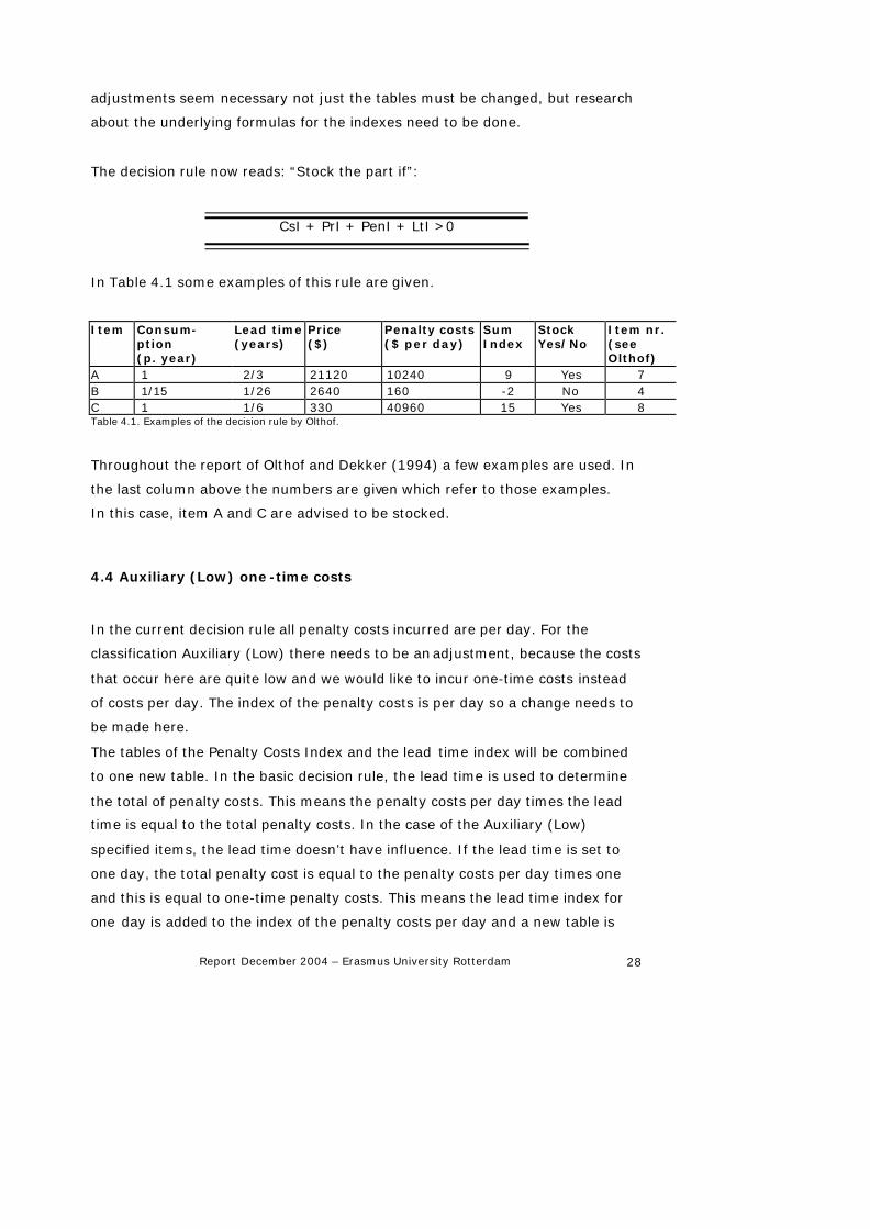
The decision rule now reads: “Stock the part if”:
CsI + PrI + PenI + LtI >0
In Table 4.1 some examples of this rule are given.
Item Consum-ption (p. year)
Lead time (years)
Price ($)
Penalty costs ($ per day)
Sum Index
Stock Yes/No
Item nr. (see Olthof)
A 1 2/3 21120 10240 9 Yes 7 B 1/15 1/26 2640 160 -2 No 4 C 1 1/6 330 40960 15 Yes 8 Table 4.1. Examples of the decision rule by Olthof.
Throughout the report of Olthof and Dekker (1994) a few examples are used. In
the last column above the numbers are given which refer to those examples.
In this case, item A and C are advised to be stocked.
4.4 Auxiliary (Low) one-time costs
In the current decision rule all penalty costs incurred are per day. For the
classification Auxiliary (Low) there needs to be an adjustment, because the costs
that occur here are quite low and we would like to incur one-time costs instead
of costs per day. The index of the penalty costs is per day so a change needs to
be made here.
The tables of the Penalty Costs Index and the lead time index will be combined
to one new table. In the basic decision rule, the lead time is used to determine
the total of penalty costs. This means the penalty costs per day times the lead
time is equal to the total penalty costs. In the case of the Auxiliary (Low)
specified items, the lead time doesn’t have influence. If the lead time is set to
one day, the total penalty cost is equal to the penalty costs per day times one
and this is equal to one-time penalty costs. This means the lead time index for
one day is added to the index of the penalty costs per day and a new table is
Report December 2004 – Erasmus University Rotterdam 29
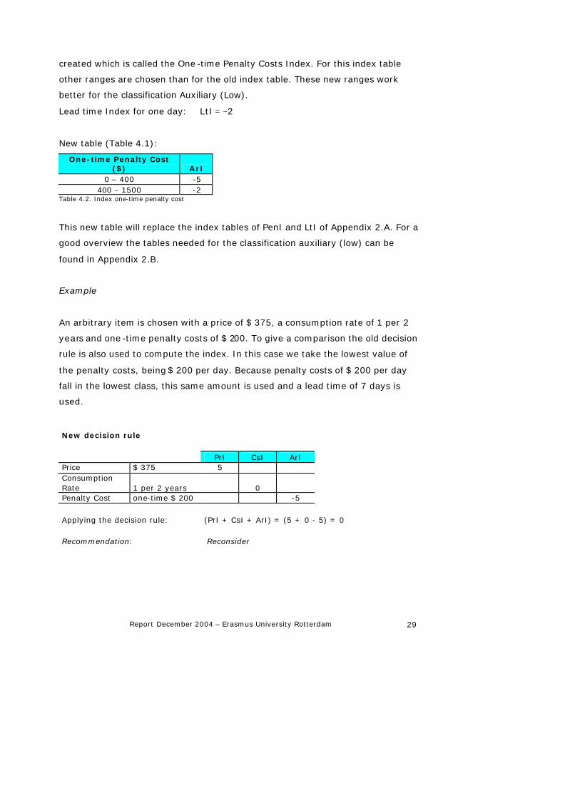
created which is called the One-time Penalty Costs Index. For this index table
other ranges are chosen than for the old index table. These new ranges work
better for the classification Auxiliary (Low).
Lead time Index for one day: 2LtI −=
New table (Table 4.1):
One-time Penalty Cost ($) ArI
0 – 400 -5 400 - 1500 -2
Table 4.2. Index one-time penalty cost
This new table will replace the index tables of PenI and LtI of Appendix 2.A. For a
good overview the tables needed for the classification auxiliary (low) can be
found in Appendix 2.B.
Example
An arbitrary item is chosen with a price of $ 375, a consumption rate of 1 per 2
years and one -time penalty costs of $ 200. To give a comparison the old decision
rule is also used to compute the index. In this case we take the lowest value of
the penalty costs, being $ 200 per day. Because penalty costs of $ 200 per day
fall in the lowest class, this same amount is used and a lead time of 7 days is
used.
New decision rule PrI CsI ArI Price $ 375 5 Consumption Rate 1 per 2 years 0 Penalty Cost one-time $ 200 -5 Applying the decision rule: (PrI + CsI + ArI) = (5 + 0 - 5) = 0 Recommendation: Reconsider
Report December 2004 – Erasmus University Rotterdam 30
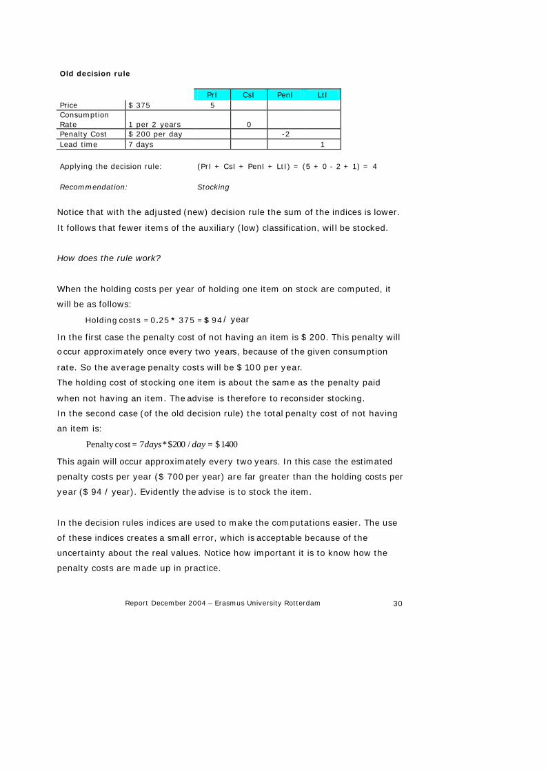
Old decision rule PrI CsI PenI LtI Price $ 375 5 Consumption Rate 1 per 2 years 0 Penalty Cost $ 200 per day -2 Lead time 7 days 1
Applying the decision rule: (PrI + CsI + PenI + LtI) = (5 + 0 - 2 + 1) = 4 Recommendation: Stocking
Notice that with the adjusted (new) decision rule the sum of the indices is lower.
It follows that fewer items of the auxiliary (low) classification, will be stocked.
How does the rule work?
When the holding costs per year of holding one item on stock are computed, it
will be as follows:
94375250costs Holding $*. == / year
In the first case the penalty cost of not having an item is $ 200. This penalty will
occur approximately once every two years, because of the given consumption
rate. So the average penalty costs will be $ 100 per year.
The holding cost of stocking one item is about the same as the penalty paid
when not having an item. The advise is therefore to reconsider stocking.
In the second case (of the old decision rule) the total penalty cost of not having
an item is:
1400$/200$*7cost Penalty == daydays
This again will occur approximately every two years. In this case the estimated
penalty costs per year ($ 700 per year) are far greater than the holding costs per
year ($ 94 / year). Evidently the advise is to stock the item.
In the decision rules indices are used to make the computations easier. The use
of these indices creates a small error, which is acceptable because of the
uncertainty about the real values. Notice how important it is to know how the
penalty costs are made up in practice.
Report December 2004 – Erasmus University Rotterdam 31
4.5 Conclusion
For the decision to stock or not to stock the decision rule of Olthof and Dekker
(1994) should be used with a few changes. First of all some definitions of the
input variables are changed, but this has no effect to the rule itself. The
classification Vital (high) and Essential (medium) still use the same rule and
index tables. In practice it is preferred to use one-time penalty costs for the
Auxiliary (low) classification. A new table is created for this last classification
Auxiliary, which replaces two tables in the old rule. The rules are still easy to
implement.

Report December 2004 – Erasmus University Rotterdam 32
5. Economic Order Quantity
5.1 Introduction
After the question to stock or not to stock, another question comes forward: how
many items need to be ordered at once. The issue at stake here is the initial
purchase at the start of a new plant. In this chapter first some general theory
about inventory models is given (section 5.2). In section 5.3 some detailed
theory about the EOQ is stated. Next something is said about the different
variables needed to compute the EOQ (section 5.4). This is followed by the
rounding of the EOQ (section 5.5), some examples (section 5.6), the maximum
period to cover (section 5.7) and finished with a short conclusion (section 5.8).
5.2 Theory
The amount of items to order at once is called the batch or order quantity Q. An
important assumption made here, is that the future demand is deterministic and
given. Deterministic demand (causally determined and not subject to random
chance ) may seem to be a very unrealistic assumption, because of the stochastic
(random) variations in demand. Also in case of stochastic demand it is often
feasible to use deterministic lot sizing. The determination of Q should, also in a
stochastic case, essentially mean that the ordering and holding costs are
balanced. A standard procedure is to first replace the stochastic demand by its
mean and use a deterministic model to determine Q. Given Q a stochastic model
is then, in a second step, used to determine the reorder point R (see chapter 6).
Why is it that, in these days of advanced information technology, many
companies are still not taking advantage of these fundamental inventory models?
Part of the answer lies in poor results received due to inaccurate data inputs.
Accurate product costs, activity costs, forecasts, history, and lead times are
crucial in making inventory models work. Software adva ncements may also in
part to blame. Many ERP packages come with built in calculations for EOQ which
(that) calculate automatically. Often the users do not understand how it is

Report December 2004 – Erasmus University Rotterdam 33
calculated and therefore do not understand the data inputs and system set-up
that controls the output. Because of this, it is simply ignored.
5.3 EOQ: theory and formula
The most well known result in the inventory control area may be the classical
Economic Order Quantity (EOQ) formula. This simple rule has had and still has
an enormous number of practical applications. The EOQ is essentially an
accounting formula that determines the point at which the combination of order
costs and holding costs are the least. The result is the most cost-effective
quantity to order. Assumptions underlying the EOQ formula are :
• Demand is constant and continuous in time .
• Ordering and holding costs are constant over time.
• The order quantity does not need to be an integer.
• The whole order quantity is delivered at the same time.
• No shortages are allowed.
These assumptions do not hold all in the case of slow moving items. In this case
an integer number of items is needed so rounding is needed (see section 5.5).
Shortages are allowed, so this assumption is released. There is also a possibility
of including q uantity discounts, but this is left out of this research.
The basic Economic Order Quantity (EOQ) formula is as follows:
( )( )( )unitper cost holding Annual
costsOrder units in usage Annual*2EOQ =
From hereon we will use symbols for this formula:
HCA2
EOQ =
where
C = Annual consumption rate in units
A = Order costs
H = Annual holding cost per unit

Report December 2004 – Erasmus University Rotterdam 34
The annual holding cost per unit H will be defined as
H = i * P
where
i = Holding cost rate
P = Purchase cost
Note that it may be possible that the EOQ formula gives a value of more than 2
while on the other hand the stocking decision is negative. This will be the case if
the order costs are high, but the criticality of the items is low. Consider for
example an auxiliary item with a stockout penalty of $ 200, which costs $ 3000
and has a consumption of 2 per year. The new decision rule gives -5 + 2 + 2 = -
1 and advises therefore not to stock. If the order costs are $ 500 per occasion ,
the EOQ, however, equals v2.6 = 1.65, which will be rounded up to 2. Notice
that by ordering 2 items after a demand instead of one, we save once a
replenishment order of $ 500, which is more than the holding cost of the second
item for half a year (0.25 x 0.5 x $ 3000 = $375). This can be considered
equivalent to a one-time penalty of $ 500 . The latter corresponds to an index of -
2, in which case the rule advises to stock.
5.4 Input variables
As can be seen above four parameters are needed to compute the EOQ. These
variables are already explained in section 2.2 and 2.3. The calculations are fairly
simple, but the task of determining the correct data inputs to accurately
represent the inventory and operation is more difficult. Exaggerated order costs
and carrying costs are common mistakes made in EOQ calculations. Accuracy
here is crucial but small variance s in the data inputs generally have very little
effect on the outputs. See Chapter 7 for a sensitivity analysis.

Report December 2004 – Erasmus University Rotterdam 35
5.5 Rounding
The EOQ will almost never give an integer answer of how many items to stock.
Because of this a rule of rounding is needed. For every number between zero and
one the batch quantity is rounded to one. For the other numbers the following
rule is used. Assume that the EOQ lies between the numbers n and n+1, that is,
n < EOQ* < n+1, where n is an integer. Since the cost function:
O*
*
EOQC
H2
EOQF +=
is convex the best choice for EOQ is either n or n +1. The right choice should be
made as follows. Choose EOQ = n if ** /)1(/ EOQnnEOQ +≤ . Otherwise, choose
EOQ = n + 1 (Axsäter, 2000).
In reality some suppliers will only offer batch quantities as a multiple of some
number. For instance, it is possible that one can order only multiples of ten
items. This means another kind of rounding is necessary. This has to be kept in
mind, but it is left out in this research.
5.6 Examples
In tables 5.1 and 5.2 one can see what this formula does.
Ordercost Purch/ item Consum/year EOQ Order quantity 36 1 4 33.94 34 36 6 4 13.86 14 36 100 0.5 1.2 1 36 100 4 3.39 3 36 1000 0.5 0.38 1
36 1000 4 1.07 1 36 2500 0.5 0.24 1 36 2500 4 0.68 1
Table 5.1. Costs and choice of rounding; Order cost is $ 36
The higher the purchase costs per item are, the lower the EOQ. This is because
the higher the holding costs are. And the higher the consumption rate is, the
higher the EOQ. Notice that an EOQ less than one is always rounded up to one.
Report December 2004 – Erasmus University Rotterdam 36
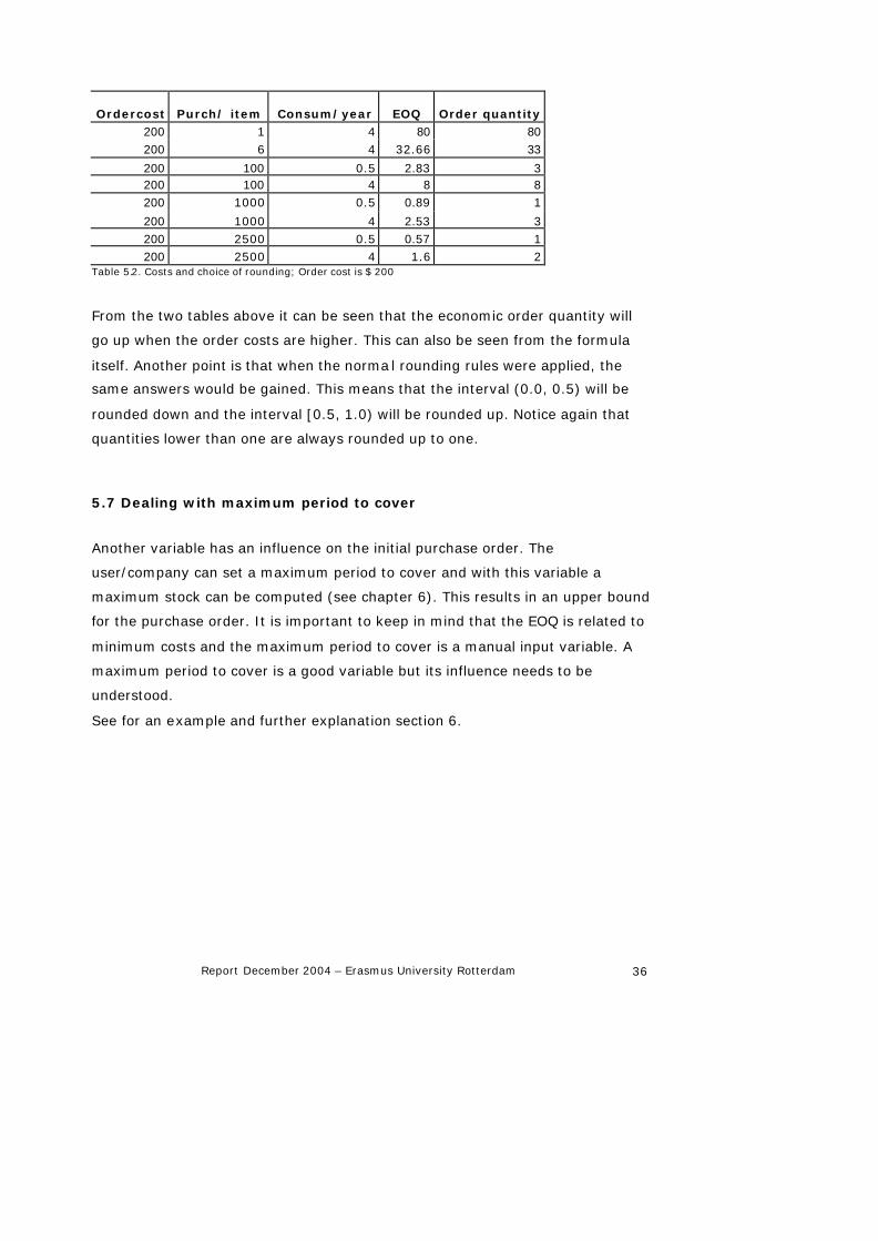
Ordercost Purch/ item Consum/year EOQ Order quantity 200 1 4 80 80 200 6 4 32.66 33
200 100 0.5 2.83 3 200 100 4 8 8 200 1000 0.5 0.89 1
200 1000 4 2.53 3 200 2500 0.5 0.57 1 200 2500 4 1.6 2
Table 5.2. Costs and choice of rounding; Order cost is $ 200
From the two tables above it can be seen that the economic order quantity will
go up when the order costs are higher. This can also be seen from the formula
itself. Another point is that when the norma l rounding rules were applied, the
same answers would be gained. This means that the interval (0.0, 0.5) will be
rounded down and the interval [0.5, 1.0) will be rounded up. Notice again that
quantities lower than one are always rounded up to one.
5.7 Dealing with maximum period to cover
Another variable has an influence on the initial purchase order. The
user/company can set a maximum period to cover and with this variable a
maximum stock can be computed (see chapter 6). This results in an upper bound
for the purchase order. It is important to keep in mind that the EOQ is related to
minimum costs and the maximum period to cover is a manual input variable. A
maximum period to cover is a good variable but its influence needs to be
understood.
See for an example and further explanation section 6.
Report December 2004 – Erasmus University Rotterdam 37
5.8 Conclusion
To create an ordering policy it is important to find an efficient order quantity. The
formula used to compute this quantity needs to be easy to use and implement.
In general it is known that many logistics companies use a simple formula known
as the Economic Order Quantity. It is easy to use in practical applications and
easy to implement in current systems. The advise here is to use this formula to
balance the ordering and holding costs.

Report December 2004 – Erasmus University Rotterdam 38
6. Minimum Stock
6.1 Introduction
An important feature in inventory control is the determination of the minimum
number of items that should be on stock. In this report the following definition of
minimum stock is used: the minimum level of inventory on stock which can be
tolerated (that is, before a replenishment order is placed). An order is placed
when the inventory level drops below this level. The level of stock at which an
order is placed is called ‘re -order point’ and is therefore the minimum stock
minus 1. Using Q for the number of items ordered at once and S for the level of
minimum stock, this strategy is also called (S-1,S+Q-1)-strategy.
In this chapter it will be explained how to determine this minimum stock. In
section 6.2 first will be explained why it is important to determine this number
and what the difficulties are. Section 6.3 will discuss three possible methods to
compute the minimum stock. The total costs of these methods will be computed
in section 6.4. Section 6.5 gives a suggestion on how to decide which method to
choose and section 6.6 will be about dealing with the maximum stock. Finally a
conclusion in section 6.7 will summarize the results of this chapter.
6.2 Determining the Minimum Stock
A company needs to decide how many items at least it wants to keep on stock.
This is an important decision because it can cost a large amount of money when
the wrong decision is made. This decision can be wrong in two ways: too much
or too little. In the first case the company holds too many items on stock and
this will result in high holding costs. In the other case there is a large probability
of needing an item when it is not on stock, which results in (high) penalty costs.
Therefore it is necessary that a company makes the best possible decision. In
this chapter methods are described to support this decision-making process.
Because there are many other terms and methods to define the number of items
on stock it is important to get clear what this chapter is dealing with.
Report December 2004 – Erasmus University Rotterdam 39
The objective is to compute the minimum level of inventory for which it is
necessary to place a new order when the stock drops below this level. The
minimum stock will be determined considering the consumption during the lead
time. This consumption gives the estimated number of items needed during the
lead time of the ordered items. When a new order is released (for example for a
number equal to the EOQ) at the moment that the inventory level reaches this
number of items it means that we would like to reach an inventory of 0 exactly
at the moment the new order arrives. This is of course the optimal strategy. But
this simple strategy is impossible to implement because the consumption is
almost never exactly known. An example will make this clear (note that the
parameters for this example are chosen for their simplicity, not because of
practical interest):
Suppose you have an item X with an estimated yearly consumption of 12 items.
The lead time of item X is 1 month. It seems to be optimal to order a new
amount of items at the moment that the inventory level drops from 2 to 1 item
(say: the minimum stock is 2 and reorder when the inventory drops below this
level). During the month the new items have not arrived there will be an
estimated consumption of 1 item (12 per year / 12 months = 1 per month) and
therefore the new items arrive exactly at the moment that there are no items X
on stock.
But what happens if during this month not 1 but 2 or 3 or more items are
consumed? This will result in a stock out with penalty costs because there are
not enough items on stock. Maybe it is less expensive to keep an extra stock of 1
or 2 items than to risk the probability of getting out of stock. So the minimum
stock of item X not only depends on the estimated consumption during the lead
time, but a lso on the probability of a higher (or lower) consumption and also on
the penalty costs and the holding costs of item X. Knowing this probability, an
estimation of the penalty and the holding costs can be made for different
minimum stock levels.
This example shows that the minimum stock depends on several factors:
1. the lead time of the part
2. the costs of keeping an item on stock

Report December 2004 – Erasmus University Rotterdam 40
3. the importance of having the part (the criticality of the equipment)
expressed (in this section) in penalty costs
4. the consumption rate of the part and the distribution of this rate
For factors 1 and 2 the values are taken as the user enters them. For factor 3
there are two methods, which will be explained in this chapter. In the next
chapter a more detailed investigation will be ma de and a recommendation will be
given. Factor 4 is the most complex factor in the determination of the minimum
stock. Therefore the next section will give an explanation of the difficulty of this
factor and a description of the methods to solve this.
6.3 Distribution of the consumption
6.3.1 Introduction
Before computing the minimum stock, a short overview of the importance of
knowing the distribution of the consumption rate will be given in this section.
The probability of needing x items has to be determined. For example, what is
the probability that the consumption of an item during the lead time will be 5, 6
or 7 items instead of an expected amount of 4? This can be different for every
company and real data is needed to compute this probability. With these
probabilities, a distribution for the consumption can be estimated. This chapter
will give a theoretical description of the minimum stock method. The minimum
stock will be computed with three different distributions to show the effect of
different distributions on the minimum stock. It is difficult to make a practical
investigation for one specific company, based on real data, because there are no
real data available, but this chapter will give a recommendation of which method
to use in which situation.
The company can choose the specific distribution that is appropriate for its
situation. In the sections 6.3.3, 6.3.4 and 6.3.5 these three methods will be
explained. But first something will be stated about the number of items replaced
at once (section 6.3.2).
Report December 2004 – Erasmus University Rotterdam 41
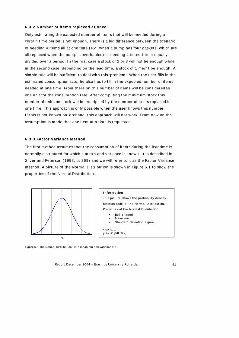
6.3.2 Number of items replaced at once
Only estimating the expected number of items that will be needed during a
certain time period is not enough. There is a big difference between the scenario
of needing 4 items all at one time (e.g. when a pump has four gaskets, which are
all replaced when the pump is overhauled) or needing 4 times 1 item equally
divided over a period. In the first case a stock of 2 or 3 will not be enough while
in the second case, depending on the lead time, a stock of 1 might be enough. A
simple rule will be sufficient to deal with this ‘problem’. When the user fills in the
estimated consumption rate, he also has to fill in the expected number of items
needed at one time. From there on this number of items will be considered as
one unit for the consumption rate. After computing the minimum stock this
number of units on stock will be multiplied by the number of items replaced in
one time. This approach is only possible when the user knows this number.
If this is not known on forehand, this approach will not work. From now on the
assumption is made that one item at a time is requested.
6.3.3 Factor Variance Method
The first method assumes that the consumption of items during the leadtime is
normally distributed for which a mean and variance is known. It is described in
Silver and Peterson (1998, p. 269) and we will refer to it as the Factor Variance
method. A picture of the Normal Distribution is shown in Figure 6.1 to show the
properties of the Normal Distribution.
mu
Figure 6.1 The Normal Distribution, with mean mu and variance = 1
Information
This picture shows the probability density
function (pdf) of the Normal Distribution.
Properties of the Normal Distribution:
• Bell-shaped • Mean mu • Standard deviation sigma
x-axis: x y-axis: pdf, f(x)
Report December 2004 – Erasmus University Rotterdam 42
This distribution can be suitable to model the consumption because this is a well-
known and widely used probability distribution function. Especially for
consumable goods, items with a coefficient of variation (standard deviation
divided by the mean) lower than 0.5 a reasonable goodness of fit is reported in a
number of applications (Minner, 2000). For slow moving items the distribution is
less suitable, because there will be a probability of negative demand. This can
simply be seen in Figure 6.1: imagine an average consumption (mu) of 1 item
and the bell-shape will be around 1 and the left part of the shape will be on the
negative side, which corresponds to a negative demand.
The formula to compute the minimum stock is:
Minimum stock = Mean consumption + (Factor * Standard deviation)
The standard deviation is the square root of the variance. In case of an initial
stock estimate no data is available. Therefore the variance (and the standard
deviation) is set at 1. The formula therefore becomes:
Minimum stock = Mean consumption + Factor
The Factor is a safety factor, when this factor is 0, for example, the minimum
stock equals the estimated mean consumption. There is always a risk of
consuming more then the estimated consumption, so the larger the safety factor,
the larger the minimum stock and the smaller the probability of a stock out. The
probability of a stock out is the probability of a higher consumption than the
minimum stock and can be computed with the help of the Normal Distribution. In
Appendix 3A is explained how this probability is computed. An example will make
this more clear. Consider an item with a consumption rate of 1 per year and a
lead time of 2 months, so the mean consumption during the lead time is 1/6
item. For different levels of minimum stock the corresponding factor and the
corresponding probability of a stock out are computed and placed in Table 6.1. A
picture of the table is shown in Figure 6.2.

Report December 2004 – Erasmus University Rotterdam 43
Minimum stock Safety Factor Probability of stock out
during lead time 0 -0.17 0.568 1 0.83 0.203 2 1.83 0.034 3 2.83 0.002
Table 6.1. Safety Factor and Probability of a Stock out during lead time for different levels of minimum stock
Example Factor Variance Method
0
0.1
0.2
0.3
0.4
0.5
0.6
0 1 2 3
Minimum stock
Pro
bab
ility
of
sto
ck o
ut
Figure 6.2 Example of the Factor Variance Method
For the different levels of minimum stock the according total costs can be
computed. The minimum stock with the lowest total costs will be chosen. How
these total costs can be computed will be discussed in the next chapter.
6.3.4 Erlang-k Method
The second method is based on the assumption that the time between two
successive demands follows an Erlang-k distribution, which is the sum of k
independent exponential distributions (so the Erlang-1 distribution is the same as
an exponential distribution). Tijms (1994) claims that any probability distribution
can be approximated by linear combinations of such distributions. This
distribution is widely used in inventory models (Minner 2000). Figure 6.3 shows a
picture of the Exponential distribution.
Information This picture shows for different levels of minimum stock the probability of a stock out during the lead time. Note that the larger the minimum stock, the smaller the probability of a stock out.

Report December 2004 – Erasmus University Rotterdam 44
Figure 6.3 The Exponential Distribution
The k factor is a factor which indicates whether the distribution is memory less.
If k=1 then an event is always equally likely to happen, even if there was no
event for a long time. The higher the k factor the more peaked the distribution
is, hence there is a low probability that two events occur quickly behind each
other. In other words, for k > 1, the spread a round the mean value will be k
times smaller than for k = 1. The larger the shape parameter k, the less variance
the distribution will have. For k growing to infinity the distribution converges to a
deterministic value. Given the value for k, the yearly consumption and the lead
time, the probability of a stock out during the lead time can be computed for
different levels of minimum stock. Details are given in Appendix 3.B. With this
probability the stock with the lowest total costs can be calculated . An example is
given to show the effect of different parameters k.
Table 6.2 gives the probabilities for an item X with a lead time of 2 months and
an estimated yearly consumption rate of 1 item. These are the probabilities of a
consumption of 0, 1, 2, 3 or 4 items during the lead time for different values of
the shape parameter of the Erlang-k distribution (k = 1 to 10). From this table
can be seen that for k = 7, 8, 9 and 10 the probabilities are almost the same.
Therefore from now on only the values for k = 1 to 7 will be taken into account.
m k=1 k=2 K=3 k=4 k=5 k=6 k=7 k=8 k=9 k=10 0 0.846 0.955 0.986 0.995 0.998 0.999 1.000 1.000 1.000 1.000 1 0.141 0.044 0.014 0.005 0.002 0.001 0.000 0.000 0.000 0.000 2 0.012 0.000 0.000 0.000 0.000 0.000 0.000 0.000 0.000 0.000 3 0.001 0.000 0.000 0.000 0.000 0.000 0.000 0.000 0.000 0.000 4 0.000 0.000 0.000 0.000 0.000 0.000 0.000 0.000 0.000 0.000
Table 6.2 Probabilities of consumption of m items for different values of k
Information This picture shows the probability density function (pdf) of the Exponential Distribution. This distribution has only positive values, so the probability of a negative value is zero. x-axis: x y-axis: pdf, f(x)
Formatted: French (France),Not Highlight
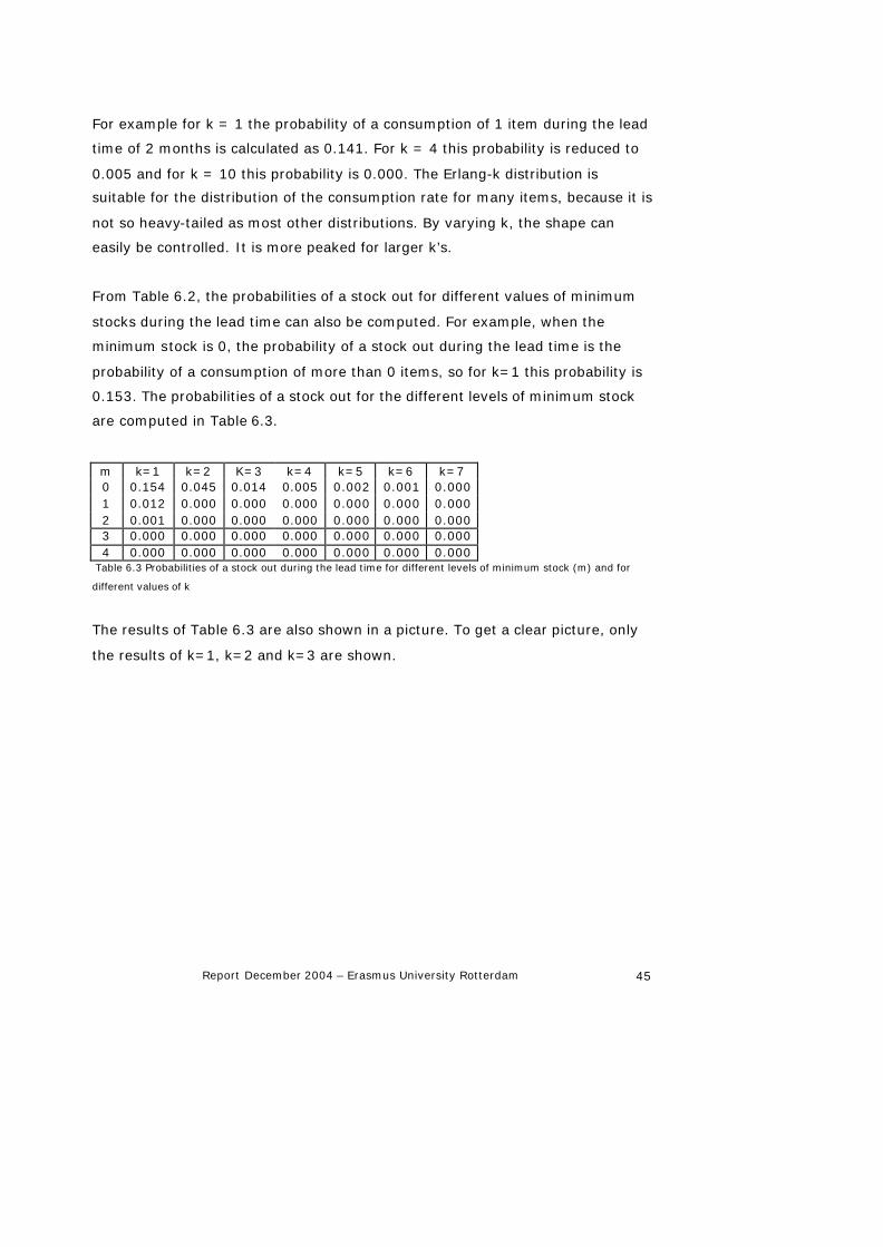
Report December 2004 – Erasmus University Rotterdam 45
For example for k = 1 the probability of a consumption of 1 item during the lead
time of 2 months is calculated as 0.141. For k = 4 this probability is reduced to
0.005 and for k = 10 this probability is 0.000. The Erlang-k distribution is
suitable for the distribution of the consumption rate for many items, because it is
not so heavy-tailed as most other distributions. By varying k, the shape can
easily be controlled. It is more peaked for larger k’s.
From Table 6.2, the probabilities of a stock out for different values of minimum
stocks during the lead time can also be computed. For example, when the
minimum stock is 0, the probability of a stock out during the lead time is the
probability of a consumption of more than 0 items, so for k=1 this probability is
0.153. The probabilities of a stock out for the different levels of minimum stock
are computed in Table 6.3.
m k=1 k=2 K=3 k=4 k=5 k=6 k=7 0 0.154 0.045 0.014 0.005 0.002 0.001 0.000 1 0.012 0.000 0.000 0.000 0.000 0.000 0.000 2 0.001 0.000 0.000 0.000 0.000 0.000 0.000 3 0.000 0.000 0.000 0.000 0.000 0.000 0.000 4 0.000 0.000 0.000 0.000 0.000 0.000 0.000
Table 6.3 Probabilities of a stock out during the lead time for different levels of minimum stock (m) and for
different values of k
The results of Table 6.3 are also shown in a picture. To get a clear picture, only
the results of k=1, k=2 and k=3 are shown.
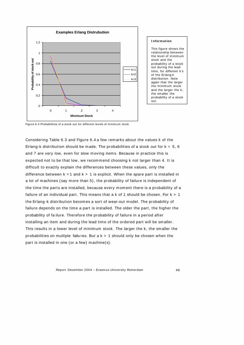
Report December 2004 – Erasmus University Rotterdam 46
Examples Erlang Distrubution
0
0.2
0.4
0.6
0.8
1
1.2
0 1 2 3 4
Minimum Stock
Pro
bab
ility
of s
tock
ou
t
k=1
k=2
k=3
Figure 6.4 Probabilities of a stock out for different levels of minimum stock
Considering Table 6.3 and Figure 6.4 a few remarks about the values k of the
Erlang-k distribution should be made. The probabilities of a stock out for k = 5, 6
and 7 are very low, even for slow moving items. Because in practice this is
expected not to be that low, we recommend choosing k not larger than 4. It is
difficult to exactly explain the differences between these values, only the
difference between k =1 and k > 1 is explicit. When the spare part is installed in
a lot of machines (say more than 5), the probability of failure is independent of
the time the parts are installed, because every moment there is a probability of a
failure of an individual part. This means that a k of 1 should be chosen. For k > 1
the Erlang-k distribution becomes a sort of wear-out model. The probability of
failure depends on the time a part is installed. The older the part, the higher the
probability of fa ilure. Therefore the probability of failure in a period after
installing an item and during the lead time of the ordered part will be smaller.
This results in a lower level of minimum stock. The larger the k, the smaller the
probabilities on mulitple failures. But a k > 1 should only be chosen when the
part is installed in one (or a few) machine(s).
Information This figure shows the relationship between the level of minimum stock and the probability of a stock out during the lead time, for different k’s of the Erlang-k distribution. Note again that the larger the minimum stock and the larger the k, the smaller the probability of a stock out.
Report December 2004 – Erasmus University Rotterdam 47
To say it simply: take a k of 1 when the purpose is to avoid any risk, or in a
situation of areas with highly uncertain logistics (for example Middle East), or
when the item is installed in many machines which are maintained
independently. Take a k of 4 in case of areas where the item is installed in a few
machines only and when the spare parts logistics is trustworthy (for example in
the Rotterdam or Houston areas).
6.3.5 Simple Minimum Stock Method
The third method is a very simple estimation of the number of needed items
during a period. This method is not a scientific method but it is often used as a
“common sense” idea. The idea of the method is to increase the lead time with a
safety factor to reach a higher level of minimum stock.
The formula is:
Minimum Stock = C * L * factor.
With C = Consumption rate and L = lead time. The factor is the minimum period
to cover (see also section 2.2.6) and can be different for the different classes of
equipment. An example will show how this method works. An item X has the
following properties: Lead time 2 months, a Consumption rate of 1 per year,
Criticality is Vital (High) with a safety factor 3 and a Purchase costs of $1000.
The minimum stock is the consumption during the lead time multiplied by the
safety factor. This computation results in a minimum stock of 1 * 1/6 * 3 = ½
item. This will be rounded to 1. This example shows an important property of this
method: the purchase costs of the item have no influence on the minimum stock.
This is the disadvantage of this method; it doesn’t take holding and penalty costs
into account. Because this method is not based on a distribution of the
consumption rate there are no calculations needed to compare the total costs for
different minimum stock levels, as in the other two methods. Therefore this
method will not return in the section about total costs computations.
6.3.6 Conclusion
In this section three different methods have been described to determine the
minimum stock level. The first is the Factor Variance Method, based on the
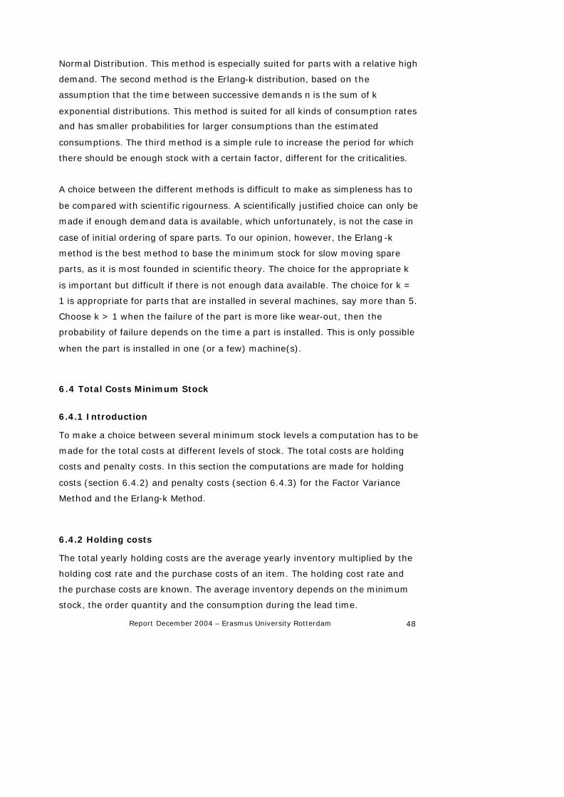
Report December 2004 – Erasmus University Rotterdam 48
Normal Distribution. This method is especially suited for parts with a relative high
demand. The second method is the Erlang-k distribution, based on the
assumption that the time between successive demands n is the sum of k
exponential distributions. This method is suited for all kinds of consumption rates
and has smaller probabilities for larger consumptions than the estimated
consumptions. The third method is a simple rule to increase the period for which
there should be enough stock with a certain factor, different for the criticalities.
A choice between the different methods is difficult to make as simpleness has to
be compared with scientific rigourness. A scientifically justified choice can only be
made if enough demand data is available, which unfortunately, is not the case in
case of initial ordering of spare parts. To our opinion, however, the Erlang-k
method is the best method to base the minimum stock for slow moving spare
parts, as it is most founded in scientific theory. The choice for the appropriate k
is important but difficult if there is not enough data available. The choice for k =
1 is appropriate for parts that are installed in several machines, say more than 5.
Choose k > 1 when the failure of the part is more like wear-out, then the
probability of failure depends on the time a part is installed. This is only possible
when the part is installed in one (or a few) machine(s).
6.4 Total Costs Minimum Stock
6.4.1 Introduction
To make a choice between several minimum stock levels a computation has to be
made for the total costs at different levels of stock. The total costs are holding
costs and penalty costs. In this section the computations are made for holding
costs (section 6.4.2) and penalty costs (section 6.4.3) for the Factor Variance
Method and the Erlang-k Method.
6.4.2 Holding costs
The total yearly holding costs are the average yearly inventory multiplied by the
holding cost rate and the purchase costs of an item. The holding cost rate and
the purchase costs are known. The average inventory depends on the minimum
stock, the order quantity and the consumption during the lead time.

Report December 2004 – Erasmus University Rotterdam 49
The average inventory can easily be computed by the following reasoning: The
average stock is the minimum stock (M) added by the order quantity (Q) divided
by a half minus the demand during the lead time (C*L). In a formula:
L*C - Q/2 M levelstock Average +=
This can be shown in a picture, see Figure 6.4. This figure shows an inventory
system of an item with a minimum stock of 2. When the stock level drops below
this minimum stock, an order of 10 items is placed and received a lead time of 2
periods later. The consumption rate is 2 items per period, so at period 4 the first
order is placed and the stock level reach the level of 10 at period 6. The average
stock level is 5 (the yellow line in Figure 6.4). This is equal to 2 + 10/2 – 2.
Figure 6.4 Example of an inventory system with Minstock is 2, Order Quantity is 10, Lead time is 2 periods and
the consumption rate is 2 per period.
Now the holding costs of the item of the example of section 6.3 will be computed
for the different methods.
Remember that this item has the following properties: Lead time 2 months, a
Consumption rate of 1 per year and Purchase costs of $ 1,000. The penalty costs
of this item with criticality Vital (High) are set at $ 30,000 per day.
The holding cost rate of 0.25/year and the purchase costs imply that the holding
cost are: 0.25/year * $1,000 per item = $ 250 per item per year. For the order
quantity the Economic Order Quantity as explained in Chapter 5 will be used. In
this example the EOQ is 1. The consumption during the lead time is 1/6 item.
Example Inventory System
0
2
4
6
8
10
12
0 1 2 3 4 5 6 7 8 9 10 11
Time
Sto
ck l
evel
Information This picture shows an example of an inventory system. The initial inventory of 10 items is decreasing over the time and when this level drops below the minimum stock of 2 an order of 10 items is placed. After a lead time these items arrive and the stock level is again 10 items, and this cycle continues.
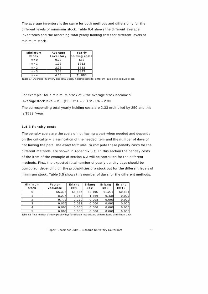
Report December 2004 – Erasmus University Rotterdam 50
The average inventory is the same for both methods and differs only for the
different levels of minimum stock. Table 6.4 shows the different average
inventories and the according total yearly holding costs for different levels of
minimum stock.
Minimum Stock
Average Inventory
Yearly holding costs
m=0 0.33 $83 m=1 1.33 $333 m=2 2.33 $583 m=3 3.33 $833 m=4 4.33 $1.083
Table 6.4 Average inventory and total yearly holding costs for different levels of minimum stock
For example: for a minimum stock of 2 the average stock become s:
2.33 1/6 - 1/2 2 L *C - Q/2 M levelstock Average =+=+=
The corresponding total yearly holding costs are 2.33 multiplied by 250 and this
is $583 /year.
6.4.3 Penalty costs
The penalty costs are the costs of not having a part when needed and depends
on the criticality + classification of the needed item and the number of days of
not having the part. The exact formulas, to compute these penalty costs for the
different methods, are shown in Appendix 3.C. In this section the penalty costs
of the item of the example of section 6.3 will be computed for the different
methods. First, the expected total number of yearly penalty days should be
computed, depending on the probabilities of a stock out for the different levels of
minimum stock. Table 6.5 shows this number of days for the different methods.
Minimum stock
Factor Variance
Erlang k=1
Erlang k=2
Erlang k=3
Erlang k=10
0 56.395 65.632 62.195 61.271 60.8341 8.274 5.058 1.369 0.438 0.0072 0.773 0.270 0.008 0.000 0.0003 0.037 0.011 0.000 0.000 0.0004 0.001 0.000 0.000 0.000 0.0005 0.000 0.000 0.000 0.000 0.000
Table 6.5 Total number of yearly penalty days for different methods and different levels of minimum stock

Report December 2004 – Erasmus University Rotterdam 51
This total number of penalty days should be multiplied by the penalty values and
this results in the total yearly penalty costs. For the different methods and levels
of minimum stock the results are shown in Table 6.6.
Minimum stock
Factor Variance
Erlang k=1
Erlang k=2
Erlang k=3 Erlang k=10
0 1,691,850 1,968,975 1,865,841 1,838,133 1,825,0091 248,231 151,754 41,081 13,142 92 23,204 8,098 241 9 03 1,097 329 1 0 04 22 11 0 0 05 0 0 0 0 0
Table 6.6 Total yearly penalty costs ($) for different methods and different levels of minimum stock
6.5 Advise
To determine the optimal minimum stock the example of the last sections will be
examined here. The total costs consist of holding and penalty costs. Therefore
Table 6.7 gives the total costs for the different levels of minimum stock for the
different methods. For every method the optimal minimum stock (with according
lowest total costs) is bold.
Minimum stock
Factor Variance
Erlang k=1
Erlang k=2
Erlang k=3
Erlang k=10
0 1,691,933 1,969,058 1,865,924 1,838,217 1,825,0931 248,564 152,087 41,414 13,475 3432 23,788 8,681 824 592 5833 1,930 1,163 834 833 8334 1,106 1,094 1,083 1,083 1,0835 1,333 1,334 1,333 1,333 1,333
Table 6.7 Total costs ($) for different levels of minimum stock for the different methods
Compare these values for the minimum stock with the computed minimum stock
of 1 item with the Simple Minimum Stock Method (as computed in section 6.3.5).
The difference is due to the high value of the penalty costs, which are not
present in the Simple Minimum Stock Method.
Report December 2004 – Erasmus University Rotterdam 52
6.6 Maximum stock
When the maximum stock (the number of expected items needed during the
maximum period to cover as described in section 2.2.7) is lower than the advised
minimum stock, an inconsistency arises. In the example of section 6.5 it could be
possible that the maximum period to cover was set at 2 years. In that case, the
maximum stock would be 2 items. However using the Erlang-1 method, the
recommended minimum stock is 4 items. What quantity should be chosen?
Choosing the maximum stock of 2 items implies neglecting the results of the
computation of the minimum stock based on total costs. On the other hand,
choosing the recommended minimum stock of 4 items can result in a large
inventory after 2 years with an associated risk of obsolescence. We recommend
to advise the lowest value in this case while giving an indication in the program
to the user that the minimum economic stock is higher. He/she can in that case
always overrun the maximum period (as that is set for a group of items, not for
a particular item). Note that we also recommend to round the maximum stock up
to 1 if the expected demand over the maximum period to cover is less than one.
6.7 Conclusion
There are several ways of determining the minimum number of items on stock.
In this chapter three are described. After evaluating these three methods one
conclusion is that the Simple Minimum Stock Method is not a good solution, when
compared with the other methods. The method does not take costs into account
and therefore often stocks too many or too few items. It is therefore strongly
suggested not to use this method in determining the minimum stock. The best
method for the determination of the minimum stock for slow moving spare parts
is the Erlang-k method. The choice for the according k is difficult to make, but
with the guidelines provided in this chapter the choice is easier to make.

Report December 2004 – Erasmus University Rotterdam 53
7. Penalty Values
7.1 Introduction
In chapter 6 the minimum stocks are determined based on the lowest total costs.
The importance of having a part on stock is expressed in penalty costs. There is
also another way to express this importance: with service levels. This chapter
will investigate the difference between these two methods. In this report penalty
costs have been chosen instead of service levels and this chapter will show why.
Therefore first the definitions of penalty costs and service levels will be explained
in section 7.2. To compare the minimum stocks based on penalty costs and
based on service levels a few examples are computed in section 7.3. Section 7.4
will explain why the method based on penalty costs is advised. Finally section 7.5
will summarize the results of this chapter.
7.2 Penalty values and Service levels
Chapter 2 gives the definition of penalty costs and chapter 6 explains how to
compute the total costs for different levels of minimum stock. The level of
minimum stock with the lowest total costs is advised. Different criticality
classifications result in different penalty values. The user/company has to give a
range of penalty values to each criticality classification, on project level. To make
it as easy as possible, pre -defined ranges are given, which the user/company can
choose from. In Table 7.1 these ranges are given.
Classification Range ($) Auxiliary 0 - 400 400 - 1,500 Essential 0 - 1,000 per day 1,000 - 7,500 per day 7,500 - 30,000 per day Vital 30,000 - 60,000 per day > 60,000 per day
Table 7.1 Pre-defined ranges for each classification
For service levels many definitions are available. In this report we define the
service level as the probability that there is no stock out du ring the lead time.

Report December 2004 – Erasmus University Rotterdam 54
This is also called the cycle service level, see e.g. Chopra and Meindl (2001). So
the service level is the probability that the consumption during the lead time is
less than the minimum stock. For different levels of minimum stock the
corresponding service levels can be computed. The minimum stock is the first
level of minimum stock for which the service level is greater than or equal to the
required service level. The required service level can be different for the different
criticalities. The following service levels might be considered:
Criticality Vital (High) – 99% or 98%
Criticality Essential (Medium) – 95%
Criticality Auxiliary (Low) – 90%
These service levels give the proportion of requests for stock items which are
satisfied on demand. It provides an indication of how well the inventory is
meeting user requirements.
7.3 Example
The question is whether the service levels as given in section 7.2 will result in
the same levels of minimum stock as with the method using the penalty costs. In
this section the minimum stock and the service level will be computed for
different items.
Because this section has the purpose to show the difference between a
computation based on penalty costs and based on service levels, there is no
need to show differences between the computations based on the different
distributions of the consumption rate. Therefore the computations in this section
will be made with the Erlang-1 method (note that the results of the Erlang-1
method are almost the same as the Factor Variance method, as shown in
Chapter 6).
For different items the minimum stock will be computed based on service levels
and based on penalty values. Most of the properties of the items are the same:
the consumption rate is 1 item per year, the lead time is 2 months, the criticality
classification is Vital (High), the yearly holding costs are 25% of the purchase

Report December 2004 – Erasmus University Rotterdam 55
costs of the item, the order costs are set at $ 75 per order. The varying property
is the price, which varies from $ 10 to $ 100,000.
The minimum stock levels for these items are shown in Table 7.2. The
computations are made as described in Chapter 6 and Appendix 3. Remember
that the criticality classification of the items is Vital (High), which means a daily
penalty value of $ 30,000 or $ 100,000 and a service level of 98% or 99%.
Penalty values ($ per day)
Service levels
Price ($) 30,000 100,000 98% 99%10 4 5 2 3
100 4 4 2 3 1,000 4 4 2 3
10,000 3 3 2 3 1,000,000 2 3 2 3 Table 7.2 Minimum stock for different prices
Table 7.2 shows that the minimum stock based on target service levels does not
depend on the item price. A minimum stock based on penalty costs will be larger
the lower the price (because the holding costs are lower for lower prices. From
the examples can be concluded that there are large differences between basing
the minimum stock on service levels and basing the minimum stock on penalty
values.
7.4 Argumentation
In this section we will argue that it is better to base the decision how many items
to stock on penalty values. The most important reason is the fact that the service
level does not take costs into account. For the expensive and for the less
expensive items the same decision will be made, only based on target service
levels and the demand rates. Another problem with service levels concerns the
period or the group of items for which the service level is computed. It is
possible, theoretically, to reach for a few items a very high service level and for a
few items a very low service level. On average this may result in the required
service level. The main reason for a lot of companies to use service levels may
be the ease of using and determining the service levels and the fact that you can
easily check the target service level with the actually reached one, but the latter

Report December 2004 – Erasmus University Rotterdam 56
does not apply for slow moving spares. To our opinion there need to be a strong
warning that these service levels may result in an inventory position that is far
from optimal with respect to total costs. Of course the use of penalty values also
has disadvantages: in general it is very difficult to estimate the real costs of not
having a part when needed. To make it easier, it is convenient to choose penalty
values for the different criticality classifications instead of for all the individual
parts.
7.5 Conclusion
In this chapter it is recommended to use penalty values instead of service levels
for determining the minimum stock, despite the difficulties in the estimation of
the penalty values. This is because the method of penalty values takes costs into
account and is therefore most suited for to the minimization of total costs.
Report December 2004 – Erasmus University Rotterdam 57
8. Sensitivity analysis
8.1 Introduction
In this chapter a sensitivity analysis is given for the Economic Order Quantity
and for the Holding Cost Rate. The analysis starts with the EOQ (section 8.2). In
that section first the sensitiveness and theory is discussed. There will be made a
distinction between the sensitivity of the order quantity Q and the different
parameters. In section 8.3 the analysis of the holding cost rate is discussed.
Finally, some conclusions are given in section 8.4.
8.2 Sensitivity analysis EOQ
A well known and important feature of the basic EOQ model is that average
inventory cost is relatively insensitive to changes in order quantity in the region
of the optimum. In practice, actual order quantities may vary from the relevant
model optimum for a number of reasons: for example, failure to make use of the
appropriate inventory control model, preference for ‘round number’ order
quantities, or error in estimating model parameters.
Silver (1998) gives a clearly and easy to follow sensitivity analysis about the
EOQ. He has shown that the costs are insensitive to errors in selecting the exact
size of a replenishment quantity. The total cost curve is quite shallow in the
neighbourhood of the EOQ (see Figure 8.1).

Report December 2004 – Erasmus University Rotterdam 58
100 200 300 400 500 600 700 800 900
50
100
150
Q (in units)
Costs ($/year)
Figure 8.1. Cost curves
This indicates that reasonable-sized deviations from the EOQ will have little
impact on the total relevant costs incurred.
It should be emphasized that the equality of the two cost components at the
point where their sum is minimized is a very special property of the particular
cost functions considered here; it certainly does not hold in general.
Mathematically, suppose a quantity Q’ is used that deviates from the EOQ
according to the following relation:
EOQpQ )1(' +=
that is, 100p is the percentage deviation of Q’ from the EOQ. The percentage
cost penalty (PCP) for using Q’ instead of the EOQ is given by
100)(
)()'(×
−=
EOQTRCEOQTRCQTRC
PCP
where TRC is the total relevant costs per unit time, that is, the sum of those
costs per unit time, which can be influenced by the given parameter. The
dimensions are $/unit time.
2/''/)'( HQQCOQTRC +=
COHEOQTRC 2)( =
Information x-axis: Quantity (in units) y-axis: Costs ($ per year) Green line: Holding costs Red line: Order costs Blue line: Total costs

Report December 2004 – Erasmus University Rotterdam 59
As shown in appendix 4,
+=
ppPCP
150
2
This expression is plotted in Figure 8.2. It is clear that even for values of p
significantly different from zero, the associated cost penalties are quite small.
-40 -30 -20 -10 10 20 30 40 50 60 70 80 90
5
10
15
20
25
Deviation in Percentages
Percentage Cost Penalty
Figure 8.2. Percentage cost penalty (PCP)
The insensitivity of total costs to the exact value of Q used has two important
implications. First, use of an incorrect value of Q can result from inaccurate
estimates of one or more of the parameters, which are used to calculate the
EOQ. Therefore, it is not worth making accurate estimates of these input
parameters if considerable effort is involved; in most cases inexpensive, crude
estimates should suffice. Second, certain order quantities may have additional
appeal over the EOQ. The shallow nature of the total cost curve indicates that
such values can be used provided that they are reasonably close to the EOQ.
Information x-axis: deviation from the EOQ (100p is the percentage deviation of Q’ from the EOQ) y-axis: Percentage Cost Penalty (PCP)
Report December 2004 – Erasmus University Rotterdam 60
8.3 Holding Cost Rate
What does it mean when the real value of i is different from the estimated value?
First some mathematical computations about this are given.
Remember the formula for the EOQ:
iPCO
HCO
EOQ22
==
Now let’s take the real value of i as x, then
where EOQ’ is the real value of the order quantity and EOQ is the order quantity
with the estimated i.
Important to know is the difference in percentages. The real EOQ differs from the
estimated one by:
%in difference100100 =−xi
If it is taken into account that i is 25%, a graph for the differences in the
economic order quantity can be drawn. In Figure 8.3 the difference in i (in
percentage points) against the difference in the order quantity (in percentages)
is presented. This means that 1 in the x-axes stands for 26% of i instead of the
estimated 25%.
EOQxi
iPCO
xi
iPixCO
QEO ∗=∗==′ 22
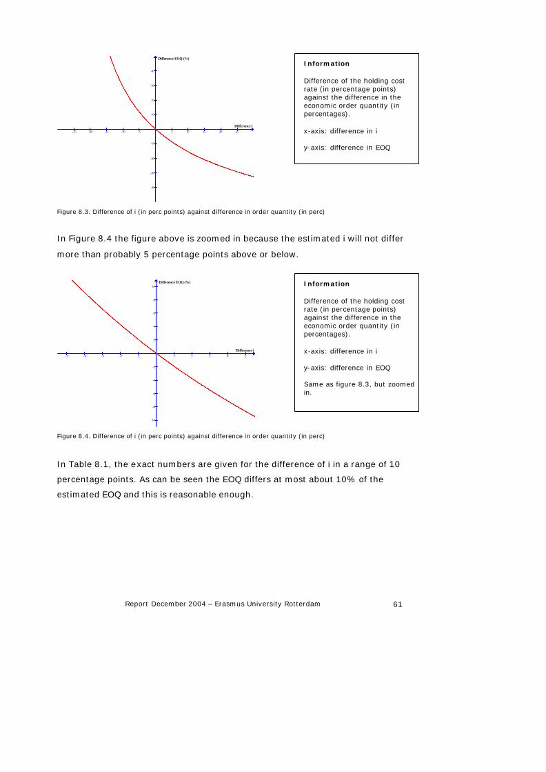
Report December 2004 – Erasmus University Rotterdam 61
-25 -20 -15 -10 -5 5 10 15 20 25
-40
-30
-20
-10
10
20
30
40
Difference i
Difference EOQ (%)
Figure 8.3. Difference of i (in perc points) against difference in order quantity (in perc)
In Figure 8.4 the figure above is zoomed in because the estimated i will not differ
more than probably 5 percentage points above or below.
- 5 - 4 - 3 -2 -1 1 2 3 4 5
-10
-8
-6
-4
-2
2
4
6
8
10
Difference i
Difference EOQ (%)
Figure 8.4. Difference of i (in perc points) against difference in order quantity (in perc)
In Table 8.1, the exact numbers are given for the difference of i in a range of 10
percentage points. As can be seen the EOQ differs at most about 10% of the
estimated EOQ and this is reasonable enough.
Information Difference of the holding cost rate (in percentage points) against the difference in the economic order quantity (in percentages). x-axis: difference in i y-axis: difference in EOQ
Information Difference of the holding cost rate (in percentage points) against the difference in the economic order quantity (in percentages). x-axis: difference in i y-axis: difference in EOQ Same as figure 8.3, but zoomed in.

Report December 2004 – Erasmus University Rotterdam 62
Table 8.1. Difference of i against the difference in EOQ
8.4 Conclusion
It can be seen from sections 8.2 and 8.3 that the Economic Order Quantity and
the Holding Cost Rate are quite robust. It is not worth making accurate estimates
of the input parameters if considerable effort is involved; in most cases
inexpensive, rough estimates should suffice.
Difference Difference
i (absolute)
EOQ (%)
(relative)
-5 11,80
-4 9,11
-3 6,60
-2 4,26
-1 2,06
1 -1,94
2 -3,77
3 -5,51
4 -7,15
5 -8,71

Report December 2004 – Erasmus University Rotterdam 63
9. Conclusions and recommendations
As stated in chapter 1 the purpose of this research is to make improvements to
the present initial spares selection procedure. For collecting information, the
standard format of the E -SPIR program is used. One of the strengths of the E-
SPIR program is the facility to advise the inventory level at the start of a plant.
Because of the lack of historical information at that moment, robust rules which
do not need that data need to be applied. Slow moving items are the most
important category of items in this respect. To improve the initial spare parts
selection procedure four main questions are answered. We shall briefly answer
each question and give recommendations when needed.
1. To stock or not to stock an item?
With some adjustments the current decision rule will still be sufficient. Th e cost
rule itself (instead of the index tables) can also be applied if computations are
done in the software package. The simple rule is mainly useful when a user
needs to make the computations himself. The main adjustments made are the
change in penalty values. In the new situation an item belongs to one of three
criticality classifications: Vital (High), Essential (Medium) or Auxiliary (Low). Next
each of these classes belongs to a range of penalty costs. The user/company
only has to choose a range for each criticality classification once, at the start of a
new plant, and subsequently has to give each item a criticality classification. In
practice it is found that for the classification Auxiliary (Low) a one-time penalty
cost will be more sufficient than costs per day. An extra possibility is given to
give zero-cost days for the classifications Vital (High) and Essential (Medium).
This is done on project level and thus needs to be given by the user/company
once, at the start of a project.
2. How many to order at once?
An item is only ordered when the first question is answered with stocking. The
economic order quantity (EOQ) is a simple formula and is one of the most well
known results in the inventory control area. It is easy to compute, needs only a
Report December 2004 – Erasmus University Rotterdam 64
few relative easy parameters and is quite robust. These are the main reasons
that this formula is chosen for computing the quantity to order at once. This is
the initial order at the start of a plant. This quantity is somewhat overshadowed
by the variable maximum period to cover. The company can enter this variable in
the E -SPIR program. As can be seen at the third question, this variable results in
a maximum stock. This means an upper bound of how many items to order. It is
important to understand the effects of this maximum period to cover.
3. When to release a new order?
A minimum stock (or reorder point) needs to be computed to know when to
release a new order. An important factor is the consumption during the lead
time. From the probability distribution of this consumption, expected penalty
costs and holding costs can be calculated. The stock with the lowest total costs
needs to be chosen. We recommend using the Erlang-k method. Which k to use
needs to be chosen by the company and this needs to be done on project level.
To make this choice as easy as possible each k to choose from is explained in
terms of expected consumption. Another decision variable also has an influence
on the minimum stock. The company can give a maximum period to cover in the
E-SPIR program. Using the given yearly consumption, this maximum period to
cover results in a maximum stock. When the consumption is low and the daily
penalty costs are high this maximum stock can be lower than the minimum stock
following from the economic optimisation. That is why the maximum stock should
always be rounded up if it is below one. Companies attach great value to this
maximum stock. We advise also to show also the minimum stock in the E-SPIR
program, so as to give the user most information.
4. How to cope with penalty values?
The minimum stock discussed above is determined based on costs. Penalty costs
express the importance of having an item on stock. It is advised to use this
method instead of fixing service levels. Total costs are ultimately more important
than just considering the expected rate of availability of an item. For the
criticality classification Vital (High) and Essential (Medium) these penalty costs
are expressed in days. For the third criticality classification Auxiliary (Low) these
Report December 2004 – Erasmus University Rotterdam 65
are one time penalty costs. On project level, each of these classifications needs
to be given a pre -defined range of costs.
Besides these four main questions it is important that all the input variables are
clear and are interpreted in the same way throughout the company. Additional
research is done on the holding cost rate. This rate is not easy to determine. A
percentage of 25% seems to be a good business practice. It is important to re -
evaluate this rate regularly, say once a few years.
Further research is possible on certain issues mentioned in this report. More
empirical research can be done on the Erlang-k, especially on which k to use in
what case. It is important to realize that this distribution can be different for
each company and for each item. Diversification is therefore possible for some
items, but this makes the inventory control system more complex. More research
can also be done on the holding cost rate and the penalty costs. One important
question is whether the same holding cost rate applies to all different items. For
the penalty costs it is important to know the costs of a failure when no spare part
is available. Are the three criticality classifications enough to include all the items
or need there to be more categories? These are some questions which can be
investigated. All this additional information will make the inventory system more
complex and should therefore only be used if considerable gains are expected.
We feel that this report establishes a good base for a better use of the inventory
control system in the E-SPIR program. It is important that the company using
this program understands the inputs and the outcome of the program to reach
the optimal inventory level. Instead of making manual decisions with respect to
inventory control, this program can be used to improve the inventory control at a
company. Expert judgment is still very important to check whether the general
rules of the program are appropriate for the individual spare parts.
Report December 2004 – Erasmus University Rotterdam 66
References
Axsäter, S. (2000). “Inventory control”: Kluwer Academic Publishers, Boston.
Botter, R. & L. Fortuin (2000), “Stocking strategy for service parts – a case
stuy”, Int. J. Oper. & Prod. Mgmt 20(6), p. 656-674.
Chopra, S., & P. Meindl (2001). “Supply chain management strategy, planning
and operations”: Prentice Hall, Upper Saddle River, NJ.
Evans, M., N. Hastings & B. Peacock (1993). “Statistical distributions”: John
Wiley & Sons, New York.
Kennedy, W.J., J. Wayne Patterson & L.D. Fredenhall (2002), “An overview of
recent literature on spare parts inventories”, Int. J. Prod. Econ. 76, p. 201-215.
Mickel, L.S. & R.L. Heim (1990), “The spares calculator: a visual aid to
provisioning”, Proceedings Annual Reliability and Maintainability Symposium, p.
410-414, IEEE.
Minner, S. (2000). “Strategic Safety Stock in Supply Chains”: Spinger-Verlag,
Berlin, New York.
Mukhopadhyay, S.K., K. Pathak, & K. Guddu (2003), “Development of Decision
Support System for Stock Control at Area Level in Mines”, IE(J) Journal-MN, 84,
p. 11-16.
Nahmias, S. (2001). “Production and operations analysis” Boston: McGraw-
Hill/Irwin.
Olthof, J.R.G.A., R. Dekker (1994). Spare parts selection procedure. Report
Econometric Institute, Erasmus Universiteit Rotterdam.
Report December 2004 – Erasmus University Rotterdam 67
Press, W.H., S.A. Teukolsky, W.T. Vetterling and B.P. Flannery (2004).
“Numerical Recipes in C++: The Art of Scientific Computing”, Cambridge
University Press, Cambridge, UK.
Relex OpSim, see http://www.relexsoftware.com/products/opsim.asp
Shell (1995). Guide to procurement and logistics management. Strategic issues.
Den Haag: Shell.
Silver, E.A., D.F. Pyke & R. Peterson (1998). “Inventory management and
production planning and scheduling” New York: Wiley.
Tijm, H.C. (1994). “Stochastic models: an algorithmic approach ” Chichester:
Wiley.
Wackerly, D.D., W. Mendenhall & R.L. Schaeffer (1996). “Mathematical statistics
with applications” Belmont: Duxbury Press

Report December 2004 – Erasmus University Rotterdam 68
Appendix 1. Formulas for the indices of the stocking decision rule
Here the formulas for the indices are given. Each index consists of a logarithm of base two of a standardised value. The choice for the standard values, which thus have index 1, has been made as to facilitate the estimation. Moreover, the standards have been chosen in such a way that an index of 0 corresponds to a indifference (and hence cost equality) between stocking and nonstocking. More information can be found in Olthof and Dekker (1994). Purchase Costs Index
dollars 10560
Costs Purchaselog PrI 2
−=
Lead time Index
−=
days 4time Leadlog LtI 2
Consumption Rate Index
−=
years 2per 1Rate nConsumptiolog CsI 2
Penalty Cost Index
−=dollars 1280
Costs Penaltylog PenI 2
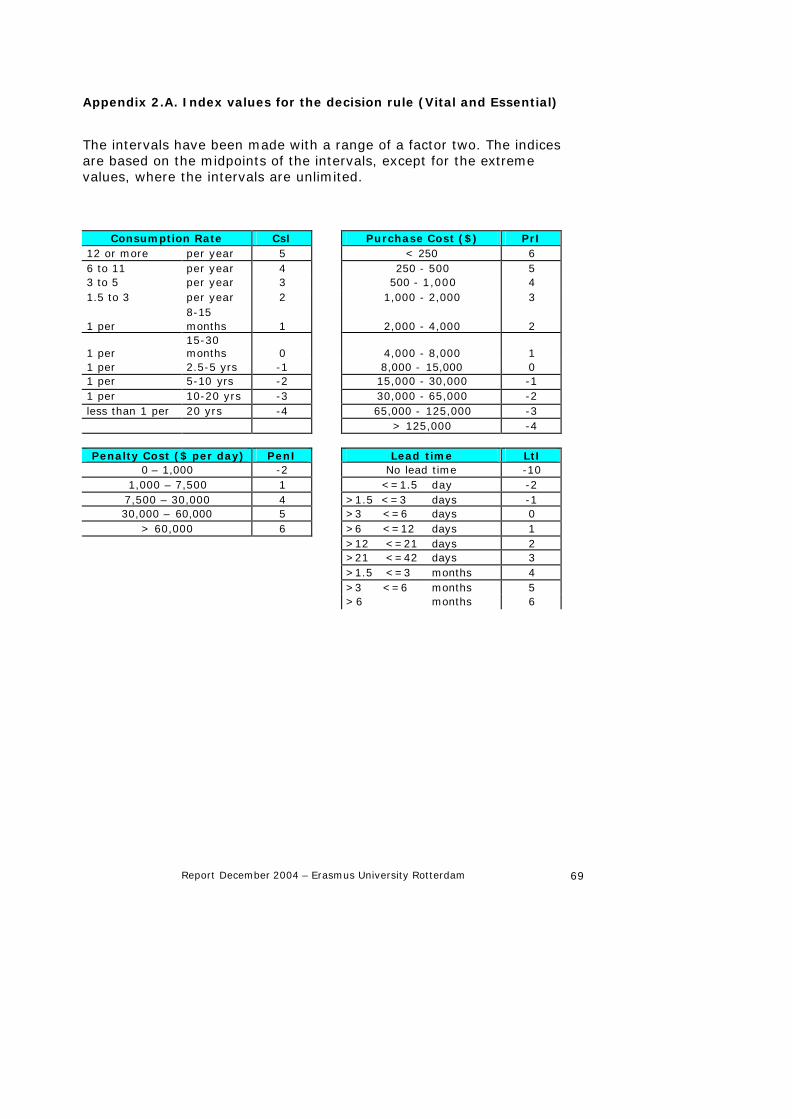
Report December 2004 – Erasmus University Rotterdam 69
Appendix 2.A. Index values for the decision rule (Vital and Essential)
The intervals have been made with a range of a factor two. The indices are based on the midpoints of the intervals, except for the extreme values, where the intervals are unlimited.
Consumption Rate CsI Purchase Cost ($) PrI 12 or more per year 5 < 250 6 6 to 11 per year 4 250 - 500 5 3 to 5 per year 3 500 - 1,000 4 1.5 to 3 per year 2 1,000 - 2,000 3
1 per 8-15 months 1 2,000 - 4,000 2
1 per 15-30 months 0 4,000 - 8,000 1
1 per 2.5-5 yrs -1 8,000 - 15,000 0 1 per 5-10 yrs -2 15,000 - 30,000 -1 1 per 10-20 yrs -3 30,000 - 65,000 -2 less than 1 per 20 yrs -4 65,000 - 125,000 -3 > 125,000 -4 Penalty Cost ($ per day) PenI Lead time LtI
0 – 1,000 -2 No lead time -10 1,000 – 7,500 1 <=1.5 day -2
7,500 – 30,000 4 >1.5 <=3 days -1 30,000 – 60,000 5 >3 <=6 days 0
> 60,000 6 >6 <=12 days 1 >12 <=21 days 2 >21 <=42 days 3 >1.5 <=3 months 4 >3 <=6 months 5 >6 months 6
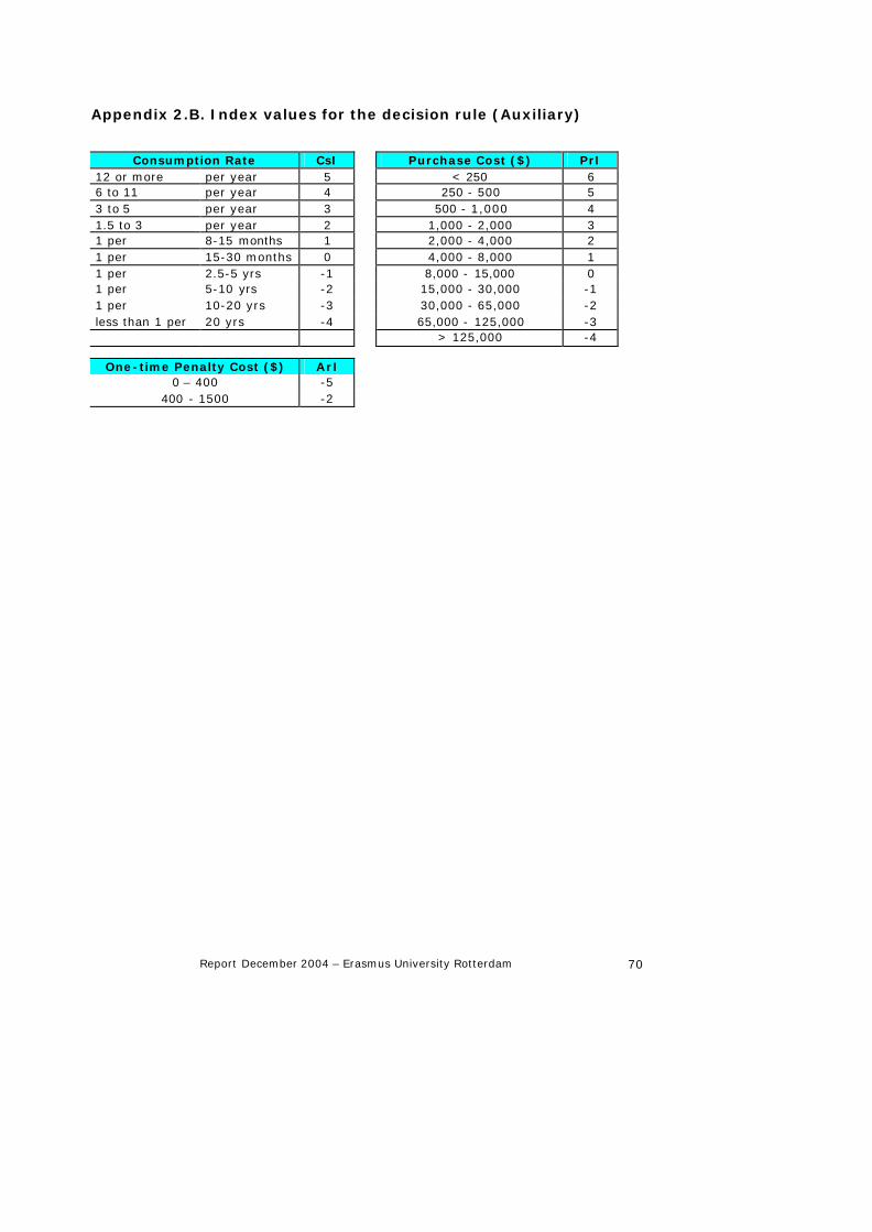
Report December 2004 – Erasmus University Rotterdam 70
Appendix 2.B. Index values for the decision rule (Auxiliary)
Consumption Rate CsI Purchase Cost ($) PrI
12 or more per year 5 < 250 6 6 to 11 per year 4 250 - 500 5 3 to 5 per year 3 500 - 1,000 4 1.5 to 3 per year 2 1,000 - 2,000 3 1 per 8-15 months 1 2,000 - 4,000 2 1 per 15-30 months 0 4,000 - 8,000 1 1 per 2.5-5 yrs -1 8,000 - 15,000 0 1 per 5-10 yrs -2 15,000 - 30,000 -1 1 per 10-20 yrs -3 30,000 - 65,000 -2 less than 1 per 20 yrs -4 65,000 - 125,000 -3 > 125,000 -4
One-time Penalty Cost ($) ArI 0 – 400 -5
400 - 1500 -2

Report December 2004 – Erasmus University Rotterdam 71
Appendix 3. Minimum Stock Computations
A Probability of Stock out for the Minimum Factor Method In this Appendix an explanation of the derivation of the formula for the
probability of a stock out in the Minimum Factor method is given. With this
method the minimum stock is computed by estimating the average consumption
during the lead time plus an extra minimum stock based on the average
variance. This variance is based on the normal distribution, with mean µ and a
variance of 1. The optimal minimum stock position, S, is equal to:
s*kµS +=
k = safety factor
µ = value of the consumption during the lead time
s = square root of the variance of the distribution of the consumption during the
lead time
If we reformulate, we get a formula for k:
sµS
k−
=
Define ? () as the cumulative distribution function of the standard Normal(0,1)
distribution. This function is directly available in e.g. Excel™ as the function
NORMDIST(.). Alternatively, good approximations are available in Press et al.
(2004). Then, the probability of a stock out during the lead time is equal to:
−
−=s
µSF1) stockout P(
If we fill in the safety factor k in this formula, we get the following equation for
the probability of a stock out during the lead time:
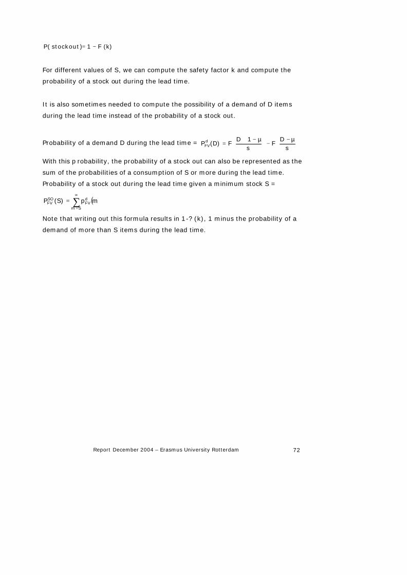
Report December 2004 – Erasmus University Rotterdam 72
F (k)1) stockout P( −=
For different values of S, we can compute the safety factor k and compute the
probability of a stock out during the lead time.
It is also sometimes needed to compute the possibility of a demand of D items
during the lead time instead of the probability of a stock out.
Probability of a demand D during the lead time =
−
−
−+
=s
µDF
sµ1D
F(D)P dFV
With this p robability, the probability of a stock out can also be represented as the
sum of the probabilities of a consumption of S or more during the lead time.
Probability of a stock out during the lead time given a minimum stock S =
( )∑∞
=
=Sm
dFV
SOFV mp(S)P
Note that writing out this formula results in 1-? (k), 1 minus the probability of a
demand of more than S items during the lead time.
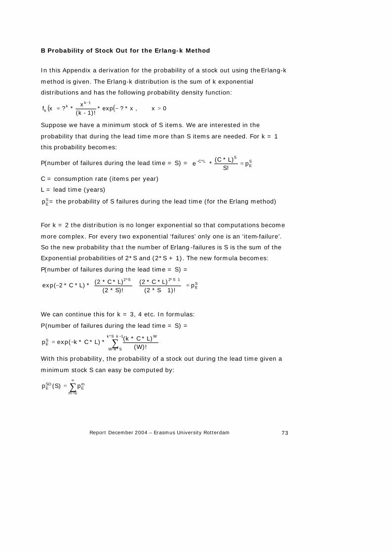
Report December 2004 – Erasmus University Rotterdam 73
B Probability of Stock Out for the Erlang-k Method
In this Appendix a derivation for the probability of a stock out using the Erlang-k
method is given. The Erlang-k distribution is the sum of k exponential
distributions and has the following probability density function:
( ) ( ) 0x ,x*?exp*1)!-(k
x*?xf
1kk
k >−=−
Suppose we have a minimum stock of S items. We are interested in the
probability that during the lead time more than S items are needed. For k = 1
this probability becomes:
P(number of failures during the lead time = S) = SE
SL*C p
S!L)*(C
*e =−
C = consumption rate (items per year)
L = lead time (years)
SEp = the probability of S failures during the lead time (for the Erlang method)
For k = 2 the distribution is no longer exponential so that computations become
more complex. For every two exponential ‘failures’ only one is an ‘item-failure’.
So the new probability tha t the number of Erlang-failures is S is the sum of the
Exponential probabilities of 2*S and (2*S + 1). The new formula becomes:
P(number of failures during the lead time = S) =
SE
1S*2S*2
p1)!S*(2
L)*C*(2S)!*(2L)*C*(2*L)*C*2exp( =
++−
+
We can continue this for k = 3, 4 etc. In formulas:
P(number of failures during the lead time = S) =
∑−+
=
−=1kS*k
S*kW
WSE (W)!
L)*C*(k*L)*C*kexp(p
With this probability, the probability of a stock out during the lead time given a
minimum stock S can easy be computed by:
∑∞
=
=Sm
mE
SOE p(S)p
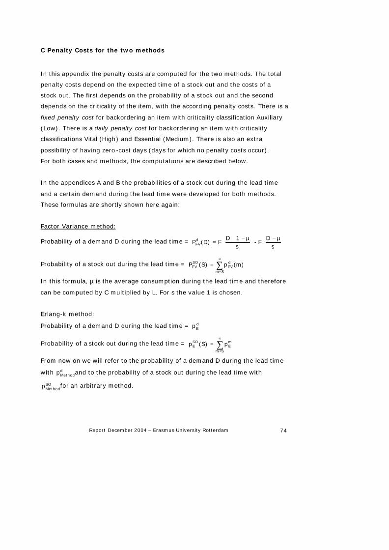
Report December 2004 – Erasmus University Rotterdam 74
C Penalty Costs for the two methods
In this appendix the penalty costs are computed for the two methods. The total
penalty costs depend on the expected time of a stock out and the costs of a
stock out. The first depends on the probability of a stock out and the second
depends on the criticality of the item, with the according penalty costs. There is a
fixed penalty cost for backordering an item with criticality classification Auxiliary
(Low). There is a daily penalty cost for backordering an item with criticality
classifications Vital (High) and Essential (Medium). There is also an extra
possibility of having zero-cost days (days for which no penalty costs occur).
For both cases and methods, the computations are described below.
In the appendices A and B the probabilities of a stock out during the lead time
and a certain demand during the lead time were developed for both methods.
These formulas are shortly shown here again:
Factor Variance method:
Probability of a demand D during the lead time =
−
−+
=s
µDF-
sµ1D
F(D)PdFV
Probability of a stock out during the lead time = ∑∞
=
=Sm
dFV
SOFV (m)p(S)P
In this formula, µ is the average consumption during the lead time and therefore
can be computed by C multiplied by L. For s the value 1 is chosen.
Erlang-k method:
Probability of a demand D during the lead time = dEp
Probability of a stock out during the lead time = ∑∞
=
=Sm
mE
SOE p(S)p
From now on we will refer to the probability of a demand D during the lead time
with dMethodp and to the probability of a stock out during the lead time with
SOMethodp for an arbitrary method.

Report December 2004 – Erasmus University Rotterdam 75
Waiting time
First two definitions are introduced:
inventory position = stock on hand + outstanding orders - backorders
inventory level = stock on hand – backorders
A demand at time T results in penalty costs when the current inventory level is
zero (so there is a stock out and a demand at that moment). To compute the
probability that this inventory level is zero, the time (T-L, T) has to be
investigated. What was the inventory level at T-L and how many items are
consumed during this time-interval? How long will the stock out endures? This
depends on the minimum stock and the order quantity. In case of an (S-1,S)-
strategy (order 1 item at the moment the inventory position drops below S) the
computation is easy. Because in this report the (S-1, S+Q-1)-strategy is used
(order an amount of Q items at the moment the inventory position drops below
S), the computation becomes a lot more complicated. Therefore the (S-1, S) -
strategy will be explained first and will be extended to the strategy as used in
this report.
A replenishment order arrives a period of L after it is ordered. Assuming that the
number of consumptions is uniformly divided over this time interval L (this is an
assumption in case of the Factor Variance method and this can be proved in case
of the Erlang-k method, as shown by Olthof and Dekker (1994, p.112)) gives an
opportunity to compute the waiting time in case of a stock out.
Suppose a failure occurs at time T and there is no stock, so there is a stock out.
Suppose that at this moment there already are B backorders. It is easy so see
that a demand at time T is backordered if and only if the number of demands in
time interval [T-L, T) is at least S, because the inventory position at any moment
is S. This means that a total of S+B items are somewhere between the supplier
and the plant. The question is how long it takes until the demand from time T will
be satisfied (the number of penalty days). This is the number of days until the
order arrives with item number B+1. Assuming that the number of consumptions
is equally divided over the lead time L, this expected penalty time (in years)
becomes B1S
1)L(B++
+ .

Report December 2004 – Erasmus University Rotterdam 76
In case of an order quantity > 1 the only difference is the total number of items
that are ordered and that not have been arrived at time T. In case of the ‘simple’
strategy, the inventory position at any moment is S. In case of an order quantity
> 1 the inventory position can be S, S+1, … , S -1+Q. After the assumption that
these positions are uniformly distributed (have equal probability) the same
reasoning can be used as the ‘simple’ strategy, but the average has to be taken
from the different inventory positions. The expected penalty time (in years)
becomes: ∑+
= +++QS
Si 1bi1)L(b
Q1 .
Finally, a formula for the total number of waiting time, given a certain S and Q
can be given as follows. The expected penalty time needs to be multiplied by the
probability that a number of S+B items is consumed during the lead time L.
Summing over all possible values of B (from zero till infinity) give the total
expected penalty time in years at a random moment of time. In formula:
Penalty time in years = ∑ ∑∞
=
+
=
+
++
+=0b
QS
Si
biMethod 1bi
1)L(b*pQ1T
Penalty costs
After computing the penalty time, the formula for the total penalty costs can be
derived for the different types of penalty values. First the case of fixed penalty
costs is given.
Let F denote the fixed penalty cost. In this case the total time of a stock out has
no influence on the total penalty costs, only the probability of a stock out and the
number of stock outs. For this computation a part of the formula for the penalty
time can be used, because that formula computes the total number of stock outs
(and multiplies this with the expected time the stock out endures, but that part is
not needed for the computation of the fixed penalty costs). This total number of
stock outs multiplied with the consumption rate and with the fixed penalty costs,
gives the total expected penalty costs per year. In formula the yearly penalty
costs in case of fixed penalty costs P f, given minimum stock S, becomes:
∑ ∑∞
=
+
=
+
=
0b
QS
Si
biMethodff p
Q1CPE
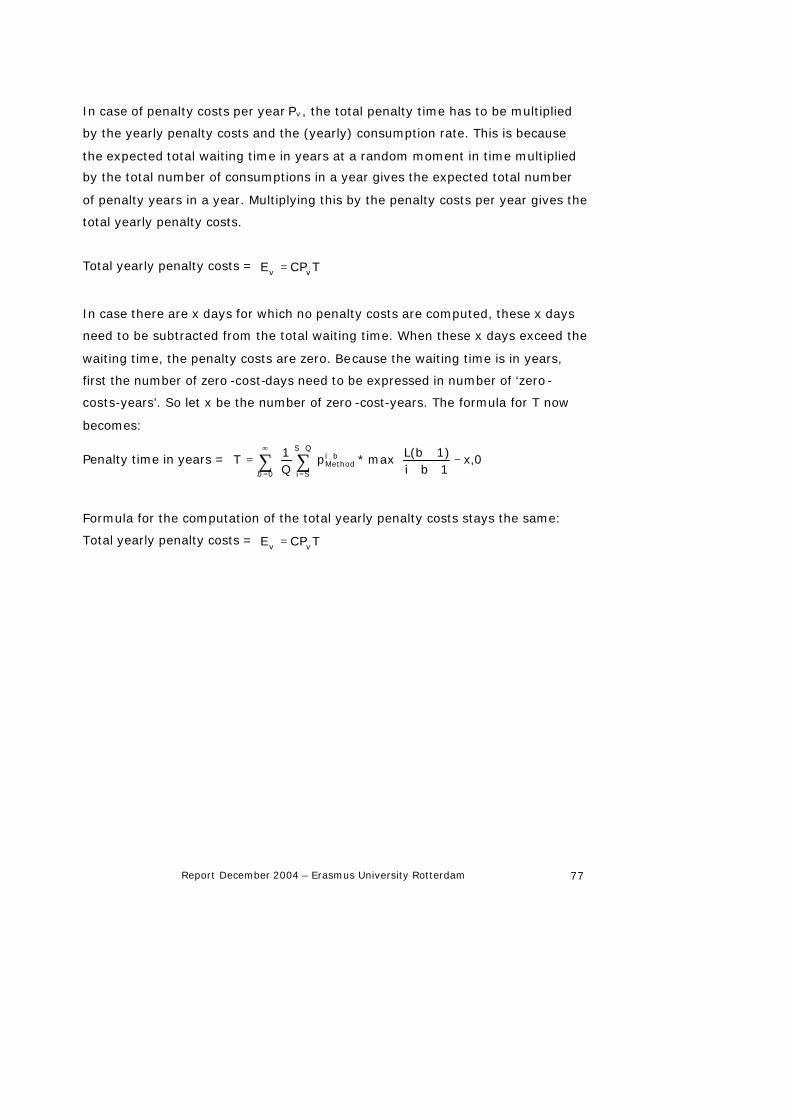
Report December 2004 – Erasmus University Rotterdam 77
In case of penalty costs per year Pv , the total penalty time has to be multiplied
by the yearly penalty costs and the (yearly) consumption rate. This is because
the expected total waiting time in years at a random moment in time multiplied
by the total number of consumptions in a year gives the expected total number
of penalty years in a year. Multiplying this by the penalty costs per year gives the
total yearly penalty costs.
Total yearly penalty costs = TCPE vv =
In case there are x days for which no penalty costs are computed, these x days
need to be subtracted from the total waiting time. When these x days exceed the
waiting time, the penalty costs are zero. Because the waiting time is in years,
first the number of zero -cost-days need to be expressed in number of ‘zero -
costs-years’. So let x be the number of zero -cost-years. The formula for T now
becomes:
Penalty time in years = ∑ ∑∞
=
+
=
+
−++
+=0
QS
Si
biMethod x,0
1bi1)L(b max*p
Q1T
b
Formula for the computation of the total yearly penalty costs stays the same:
Total yearly penalty costs = TCPE vv =
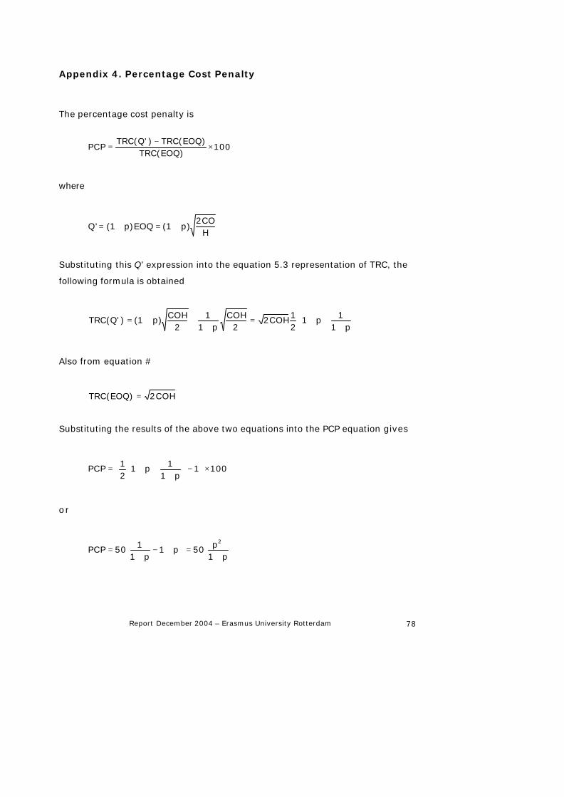
Report December 2004 – Erasmus University Rotterdam 78
Appendix 4. Percentage Cost Penalty
The percentage cost penalty is
100TRC(EOQ)
TRC(EOQ))TRC(Q'PCP ×
−=
where
H
2COp)(1p)EOQ(1Q' +=+=
Substituting this Q’ expression into the equation 5.3 representation of TRC, the
following formula is obtained
+
++=+
++=p1
1p1212COH
2COH
p11
2COHp)(1)TRC(Q'
Also from equation #
2COHTRC(EOQ) =
Substituting the results of the above two equations into the PCP equation gives
1001p1
1p121PCP ×
−
+
++=
or
+=
+−
+=
p1p50p1
p1150PCP
2