Optimal selection of Suppliers in a Supply Chain Network with Multiple Bidders · PDF...
21
POMS Abstract Acceptance - 020-0451 Abstract Title - Optimal selection of Suppliers in a Supply Chain Network with Multiple Bidders for Each stage Author 1: Shashank Garg Handheld Solutions & Research Labs 36, 20 th Main 1 st Cross, 1 st Stage BTM Layout, Bangalore – 560068 [India] Email: [email protected] Tel: +91-80-26685035 Author 2: D. Krishna Sundar Indian Institute of Management Bangalore Bannerghatta Road, Bangalore – 560076 [India] Email: [email protected] Tel: +91-80-26993276 POMS 22 nd Annual Conference Reno, Nevada, USA April 29 to May 2, 2011 Abstract In a cost competitive commodity market, procurement of raw materials, production and supply of finished goods at minimum cost plays a vital role in managing an efficient supply chain. It becomes complex while dealing with agricultural products, where procurement of raw material(s) is seasonal, production is partly seasonal where as finished product’s demand is steady throughout the year. Further complications arise when changes come in the set of service providers (supply side & distribution side) & their commercial contracts, annually. This paper models such a supply chain as a project network in which multiple time-cost bids are provided by multiple suppliers for each stage/node of the network. Market intelligence curves are developed for each stage/activity to determine the baseline cost-time solution for the network. Optimal set of suppliers is determined using the market intelligence curves and suppliers’ actual bids by formulating the problem as a linear programming problem. Keywords: Supplier Selection, Supply Chain Networks, Market intelligence curves, Optimization
-
Upload
trinhnguyet -
Category
Documents
-
view
214 -
download
0
Transcript of Optimal selection of Suppliers in a Supply Chain Network with Multiple Bidders · PDF...
POMS Abstract Acceptance - 020-0451
Abstract Title - Optimal selection of Suppliers in a Supply Chain
Network with Multiple Bidders for Each stage
Author 1: Shashank Garg Handheld Solutions & Research Labs 36, 20th Main 1st Cross, 1st Stage BTM Layout, Bangalore – 560068 [India]
Email: [email protected] Tel: +91-80-26685035
Author 2: D. Krishna Sundar Indian Institute of Management Bangalore Bannerghatta Road, Bangalore – 560076 [India] Email: [email protected] Tel: +91-80-26993276
POMS 22nd Annual Conference Reno, Nevada, USA April 29 to May 2, 2011
Abstract In a cost competitive commodity market, procurement of raw materials, production and supply of finished goods at minimum cost plays a vital role in managing an efficient supply chain. It becomes complex while dealing with agricultural products, where procurement of raw material(s) is seasonal, production is partly seasonal where as finished product’s demand is steady throughout the year. Further complications arise when changes come in the set of service providers (supply side & distribution side) & their commercial contracts, annually. This paper models such a supply chain as a project network in which multiple time-cost bids are provided by multiple suppliers for each stage/node of the network. Market intelligence curves are developed for each stage/activity to determine the baseline cost-time solution for the network. Optimal set of suppliers is determined using the market intelligence curves and suppliers’ actual bids by formulating the problem as a linear programming problem. Keywords: Supplier Selection, Supply Chain Networks, Market intelligence curves, Optimization
020-0451
Optimal selection of Suppliers in a Supply Chain Network with Multiple
Bidders for Each stage
Abstract
In a cost competitive commodity market, procurement of raw materials,
production and supply of finished goods at minimum cost plays a vital role in managing
an efficient supply chain. It becomes complex while dealing with agricultural products,
where procurement of raw material(s) is seasonal, production is partly seasonal where as
finished product’s demand is steady throughout the year. Further complications arise
when changes come in the set of service providers (supply side & distribution side) and
their commercial contracts, annually. This paper models such a supply chain as a project
network in which multiple time-cost bids are provided by multiple suppliers for each
stage/node of the network. Market intelligence curves are developed for each
stage/activity to determine the baseline cost-time solution for the network. Optimal set of
suppliers is determined using the market intelligence curves and suppliers’ actual bids by
formulating the problem as a linear programming problem.
Keywords: Supplier Selection, Supply Chain Networks, Market intelligence curves, Optimization

1. Introduction
Management of an efficient supply chain in the agro-products market requires that
procurement of raw materials, production and supply of finished goods be done at
minimum cost and within time constraints since the raw materials are of perishable
nature. Dealing with agricultural products is complex because procurement of raw
materials is often seasonal, production is partly seasonal whereas the demand for the
finished product demand is steady throughout the year. The set of service providers and
suppliers also changes periodically, resulting in fresh negotiations and contracts every
time. A project is often defined as consisting of specified sets of activities to be executed
as a one-time set of activities. Since in an agro-products supply chain a re-assessment of a
potentially new set of suppliers for a specified set of services is required every year or at
some other periodic interval, the task of optimal supplier selection can be treated as a
fresh project every time. It is for this reason that we use a project activity network as our
model for time-cost optimization.
In the literature a project has been defined in terms of events and activities to
provide a mathematical basis for critical-path planning and scheduling Kelley &
Walker(1959), Kelley(1961). Elmaghraby(1977) defines a project as a medium or large-
scale undertaking consisting of a range of activities requiring the consumptions of
varying types of resources over the entire duration of the set of activities that compose a
project. The concept of a project as being one of its kind and limited by a beginning and
an end, in contrast with the typical assembly-line production which constitutes a set of
activities repeated over a long period of time has been highlighted by Elmaghraby(1977).
Resource optimization in project activity networks has been studied by many authors. See
Parikh & Jewell(1965), Parikh & Jewell(1965), Golenko-Ginzburg(1989), Drexl(1991),
Demeulemeester(1995) and Golenko-Ginzburg & Blokh(1997). Optimization techniques
have been extensively used in the agriculture sector to provide improvement in various
aspects such as harvesting, transportation, agricultural production etc. Balm(1980) has
discussed linear programming models for application in Scottish agriculture.
Sargent(1980) has studied the impact of optimization techniques on agricultural
production. Optimization techniques have also been applied to increase sugar production
in the Australian context by Jiao, Higgins et al.(2005). Modeling techniques in the sugar
supply chain have been extensively discussed by Higgins, Beashel et al.(2006).
Scheduling and optimization of transport in the sugar sector has been discussed by
Higgins(2006), and Higgins & Laredo(2006). A production scheduling case study of a
South African sugar mill is provided in Le Gal, Lyne et al.(2008). The applicability of
decision support systems for the management of the sugar-cane supply chain has been
discussed by Lejars, Le Gal et al.(2008). Colin(2008) has used mathematical
programming models to develop strategies for the optimal management of land usage for
the sugarcane crop cycle to prevent land overuse. A comprehensive review of the
planning models used in the agriculture supply-chain has been provided by Ahumada &
Villalobos(2007). Useful insight into “transaction cost economics” in the sugar supply
chain in the Australian sugar industry was provided by Banarjee & McGovern(2004).
The design of performance metrics for measurement of efficiency in the supply chain was
studied by Baiman, Fischer et al.(2001). Strategies for replacement of inventory to gain
competitive advantage in the supply chain have been discussed by Borgman &
Rachan(2007). An overview of the modeling and analysis techniques used in the
management of manufacturing supply chains has been covered by Gunasekaren, Macbeth
et al.(2000).
The remainder of the paper is organized as follows: Section 2 describes the
proposed project activity network model for an agro-product supply chain. Market
intelligence curves are developed in section 3. This provides a baseline approximation for
the minimum time and minimum cost for a project, though it does not help in selecting
the most optimal supplier set. Extrapolation of bids using linear programming is
developed in Section 4 and Section 5 presents the results for an experimental data-set of
supplier bids for a small activity network representing the scenario in an agro-product
supply-chain. In Section 5 we conclude with suggestions for further improvements in the
optimization model.
2. Modelling an Agro-product Supply Chain
In this paper, we model an agro-product supply chain as a project network in which
multiple time-cost bids are provided by multiple suppliers for each stage or node in the
network. At each stage of the project, there are a host of suppliers or service providers
who provide widely varying bids for their products or services. The value of a bid is
dependent on the time of execution for that service. In general, if a particular service is to
be executed in a shorter time then the cost for that service will be higher than the cost of
the same service if it is performed at a slower pace. Therefore, each supplier can be
expected to provide multiple time-cost bids for the same service. Since procurement of
services for the project involves multiple inter-related activities, arriving at an optimal
selection of suppliers is non-trivial. When the project can be modeled as an activity
network involving tasks that have to be done in a particular sequence, then it should be
feasible to determine all the critical paths and the optimal supplier set.
The critical path of an activity network is the path which takes the longest time to
complete i.e. the summation of duration of all the activities falling in that path is the
largest of all other paths. The nodes falling in a critical path have a property that their
earliest realization time and latest realization time are same. Hence slack at these nodes
(or events) is zero. The activities and events falling in the critical path have to be
completed within whatever time is assigned to them, whereas events and activities in
other paths can be given a delay which should not be more than the slack available to
them. Otherwise the activities ahead of them will get delayed.
In an agro-product’s supply chain, each activity in the network model represents
some quantum of work to be done for which there are multiple suppliers who can supply
materials, resources or skills. Suppliers bid for each activity individually and each
supplier is asked to offers multiple cost-time bids for each activity. These supplier bids
generally fall into a convex curve such that cost of service decreases as time increases.
While discrete cost-time bids are offered, in reality the suppliers bids can be treated as
stochastic because suppliers can deviate from their time bids with a Gaussian probability
distribution which has mean equal to the time bid as specified and some standard
deviation. This standard deviation is typically derived based on past experience with this
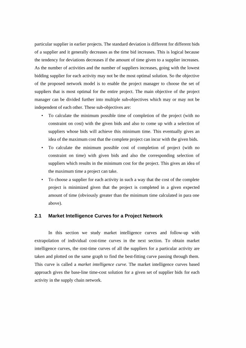
particular supplier in earlier projects. The standard deviation is different for different bids
of a supplier and it generally decreases as the time bid increases. This is logical because
the tendency for deviations decreases if the amount of time given to a supplier increases.
As the number of activities and the number of suppliers increases, going with the lowest
bidding supplier for each activity may not be the most optimal solution. So the objective
of the proposed network model is to enable the project manager to choose the set of
suppliers that is most optimal for the entire project. The main objective of the project
manager can be divided further into multiple sub-objectives which may or may not be
independent of each other. These sub-objectives are:
• To calculate the minimum possible time of completion of the project (with no
constraint on cost) with the given bids and also to come up with a selection of
suppliers whose bids will achieve this minimum time. This eventually gives an
idea of the maximum cost that the complete project can incur with the given bids.
• To calculate the minimum possible cost of completion of project (with no
constraint on time) with given bids and also the corresponding selection of
suppliers which results in the minimum cost for the project. This gives an idea of
the maximum time a project can take.
• To choose a supplier for each activity in such a way that the cost of the complete
project is minimized given that the project is completed in a given expected
amount of time (obviously greater than the minimum time calculated in para one
above).
2.1 Market Intelligence Curves for a Project Network
In this section we study market intelligence curves and follow-up with
extrapolation of individual cost-time curves in the next section. To obtain market
intelligence curves, the cost-time curves of all the suppliers for a particular activity are
taken and plotted on the same graph to find the best-fitting curve passing through them.
This curve is called a market intelligence curve. The market intelligence curves based
approach gives the base-line time-cost solution for a given set of supplier bids for each
activity in the supply chain network.
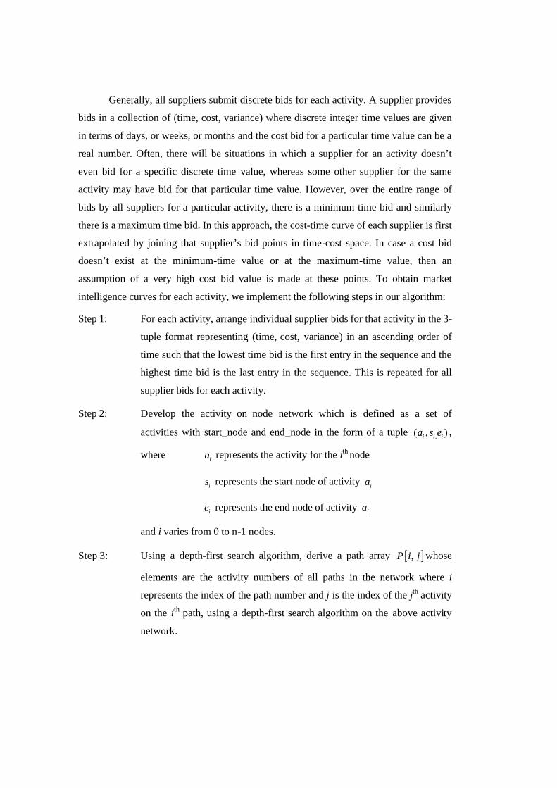
Generally, all suppliers submit discrete bids for each activity. A supplier provides
bids in a collection of (time, cost, variance) where discrete integer time values are given
in terms of days, or weeks, or months and the cost bid for a particular time value can be a
real number. Often, there will be situations in which a supplier for an activity doesn’t
even bid for a specific discrete time value, whereas some other supplier for the same
activity may have bid for that particular time value. However, over the entire range of
bids by all suppliers for a particular activity, there is a minimum time bid and similarly
there is a maximum time bid. In this approach, the cost-time curve of each supplier is first
extrapolated by joining that supplier’s bid points in time-cost space. In case a cost bid
doesn’t exist at the minimum-time value or at the maximum-time value, then an
assumption of a very high cost bid value is made at these points. To obtain market
intelligence curves for each activity, we implement the following steps in our algorithm:
Step 1: For each activity, arrange individual supplier bids for that activity in the 3-
tuple format representing (time, cost, variance) in an ascending order of
time such that the lowest time bid is the first entry in the sequence and the
highest time bid is the last entry in the sequence. This is repeated for all
supplier bids for each activity.
Step 2: Develop the activity_on_node network which is defined as a set of
activities with start_node and end_node in the form of a tuple ,( , )i i ia s e ,
where ia represents the activity for the ith node
is represents the start node of activity ia
ie represents the end node of activity ia
and i varies from 0 to n-1 nodes.
Step 3: Using a depth-first search algorithm, derive a path array [ ],P i j whose
elements are the activity numbers of all paths in the network where i
represents the index of the path number and j is the index of the jth activity
on the ith path, using a depth-first search algorithm on the above activity
network.
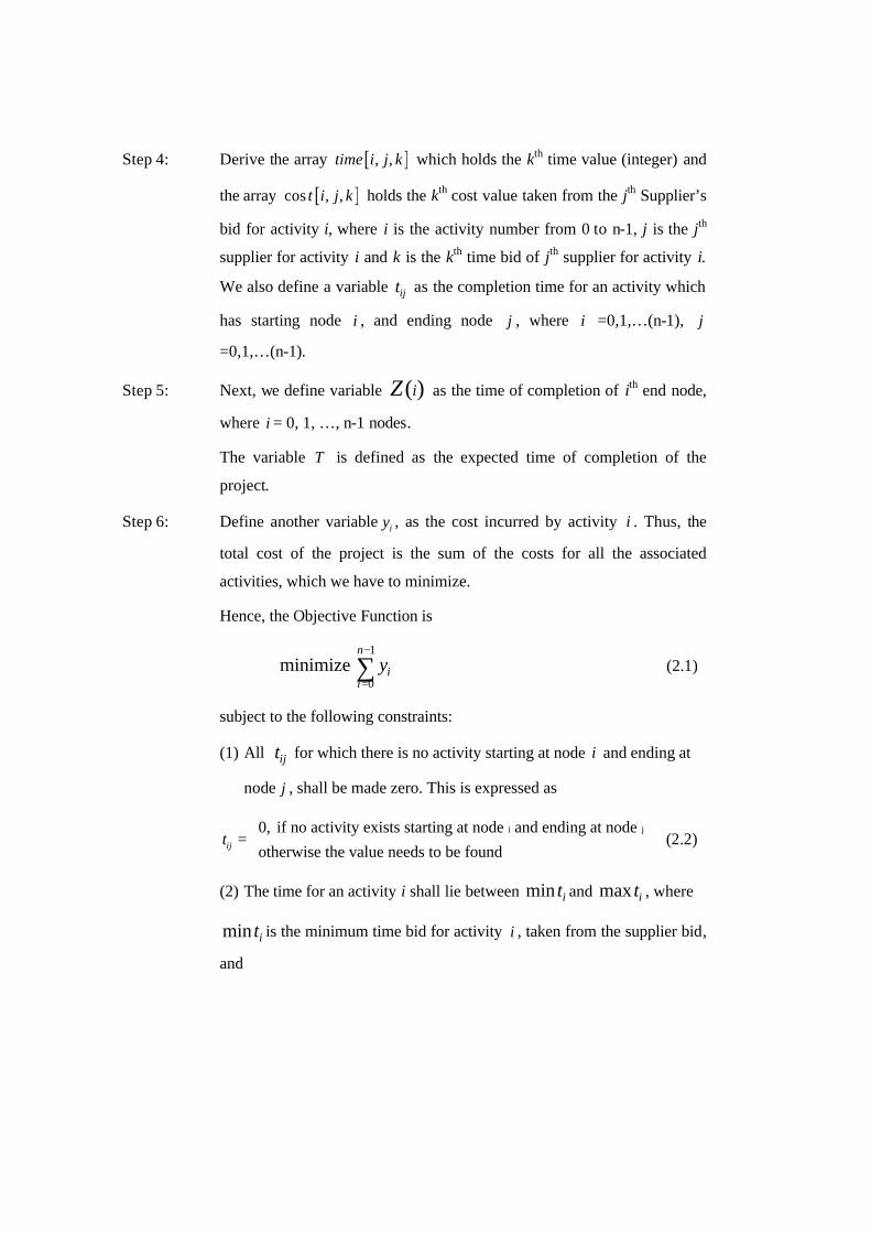
Step 4: Derive the array [ ], ,time i j k which holds the kth time value (integer) and
the array [ ]cos , ,t i j k holds the kth cost value taken from the jth Supplier’s
bid for activity i, where i is the activity number from 0 to n-1, j is the jth
supplier for activity i and k is the kth time bid of jth supplier for activity i.
We also define a variable ijt as the completion time for an activity which
has starting node i , and ending node j , where i =0,1,…(n-1), j
=0,1,…(n-1).
Step 5: Next, we define variable ( )iZ as the time of completion of ith end node,
where i = 0, 1, …, n-1 nodes.
The variable T is defined as the expected time of completion of the
project.
Step 6: Define another variable iy , as the cost incurred by activity i . Thus, the
total cost of the project is the sum of the costs for all the associated
activities, which we have to minimize.
Hence, the Objective Function is
1
0minimize
n
ii
y−
=∑ (2.1)
subject to the following constraints:
(1) All ijt for which there is no activity starting at node i and ending at
node j , shall be made zero. This is expressed as
i j0, if no activity exists starting at node and ending at node otherwise the value needs to be foundijt
=
(2.2)
(2) The time for an activity i shall lie between min it and max it , where
min it is the minimum time bid for activity i , taken from the supplier bid,
and

max it is the maximum time bid for activity i , taken from the supplier
bid.
Hence, this constraint is defined as
,min ( ) ( )i i ii s e et t Z≤ ≤ (2.3)
(3) Time for completion of starting node of an activity i plus activity time
should be less than or equal to time of completion of ending node of
that activity. Hence,
,( ) ( ) ( )i i i is s e etZ Z+ ≤ (2.4)
(4) Time for completion of terminal node should be less than or equal to
the expected time of completion of the project. Hence,
( )1nZ T− ≤ (2.5)
The above algorithm is then implemented in the following steps:
Step 1: Using the best-fitting curve function tAe λ− as an approximation which is applied to all supplier bids for each activity, we obtain market intelligence parameters ( ),i iA λ .
Step 2: Find max it , the maximum time bid for activity i and min it , the minimum time bid for activity i .
Step 3: Let ( ) ti iy t A e λ−= be the cost function for activity i on the time variable t
which represents the time taken for the activity i starting at node is and ending at node ie .
Step 4: 1
0minimize
n
ii
y−
=∑ subject to constraints in equations (2.2), (2.3), (2.4) and
(2.5) above.
3. Linear Programming Model for a Project Network

As already mentioned, over the entire range of bids by all suppliers for a
particular activity, there is a minimum time bid and similarly there is a maximum time
bid. In this approach, the cost-time curve of each supplier is first extrapolated by joining
that supplier’s bid points in time-cost space. In case a cost bid doesn’t exist at the
minimum-time value or at the maximum-time value, then an assumption of a very high
cost bid value is made at these points. Once extrapolated cost-time curves are available
for each supplier, another cost-time curve is obtained as an “envelope curve” such that
for each time bid, starting with the minimum-time value to the maximum-time value, the
minimum-cost bid is selected out of all cost bids available at that particular time value
from extrapolated curves of all suppliers for that particular activity. This gives rise to a
new cost-time curve which is used in selecting the winning suppliers.
The linear programming model is implemented in the following steps in our
algorithm:
Step 1: For each activity, arrange individual supplier bids for that activity in the 3-
tuple format representing (time, cost, variance) in an ascending order of
time such that the lowest time bid is the first entry in the sequence and the
highest time bid is the last entry in the sequence. This is repeated for all
supplier bids for each activity.
Step 2: Develop the activity_on_node network which is defined as a set of activities with start_node and end_node in the form of a tuple ,( , )i i ia s e ,
where ia represents the activity for the ith node
is represents the start node of activity ia
ie represents the end node of activity ia
and i varies from 0 to n-1 nodes.
Step 3: Using a depth-first search algorithm, derive a path array [ ],P i j whose
elements are the activity numbers of all paths in the network where i
represents the index of the path number and j is the index of the jth activity
on the ith path, using a depth-first search algorithm on the above activity
network.
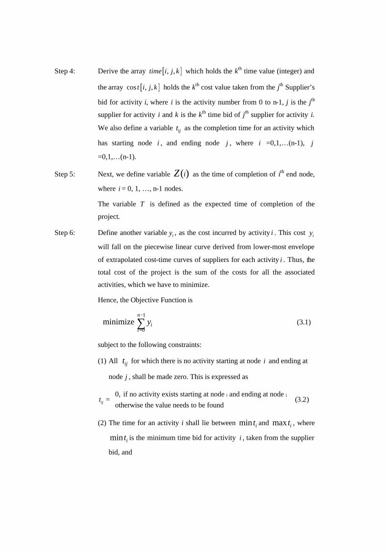
Step 4: Derive the array [ ], ,time i j k which holds the kth time value (integer) and
the array [ ]cos , ,t i j k holds the kth cost value taken from the jth Supplier’s
bid for activity i, where i is the activity number from 0 to n-1, j is the jth
supplier for activity i and k is the kth time bid of jth supplier for activity i.
We also define a variable ijt as the completion time for an activity which
has starting node i , and ending node j , where i =0,1,…(n-1), j
=0,1,…(n-1).
Step 5: Next, we define variable ( )iZ as the time of completion of ith end node,
where i = 0, 1, …, n-1 nodes.
The variable T is defined as the expected time of completion of the
project.
Step 6: Define another variable iy , as the cost incurred by activity i . This cost iy
will fall on the piecewise linear curve derived from lower-most envelope
of extrapolated cost-time curves of suppliers for each activity i . Thus, the
total cost of the project is the sum of the costs for all the associated
activities, which we have to minimize.
Hence, the Objective Function is
1
0minimize
n
ii
y−
=∑ (3.1)
subject to the following constraints:
(1) All ijt for which there is no activity starting at node i and ending at
node j , shall be made zero. This is expressed as
i j0, if no activity exists starting at node and ending at node otherwise the value needs to be foundijt
=
(3.2)
(2) The time for an activity i shall lie between min it and max it , where
min it is the minimum time bid for activity i , taken from the supplier
bid, and
max it is the maximum time bid for activity i , taken from the supplier
bid.
Hence, this constraint is defined as
,min ( ) ( )i i ii s e et t Z≤ ≤ (3.3)
(3) Time for completion of starting node of an activity i plus activity time
should be less than or equal to time of completion of ending node of
that activity. Hence,
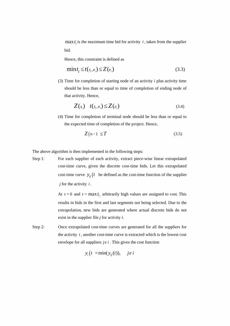
,( ) ( ) ( )i i i is s e etZ Z+ ≤ (3.4)
(4) Time for completion of terminal node should be less than or equal to
the expected time of completion of the project. Hence,
( )1nZ T− ≤ (3.5)
The above algorithm is then implemented in the following steps:
Step 1: For each supplier of each activity, extract piece-wise linear extrapolated
cost-time curve, given the discrete cost-time bids. Let this extrapolated
cost-time curve ( )ijy t be defined as the cost-time function of the supplier
j for the activity i .
At 0t = and t = max it , arbitrarily high values are assigned to cost. This
results in bids in the first and last segments not being selected. Due to the
extrapolation, new bids are generated where actual discrete bids do not
exist in the supplier file j for activity i.
Step 2: Once extrapolated cost-time curves are generated for all the suppliers for
the activity i , another cost-time curve is extracted which is the lowest cost
envelope for all suppliers j iε . This gives the cost function
( ) min( ( )),i ijy t y t j iε= ∀
This lower-most envelope represents the cost-time, piece-wise linear function for activity i.
Step 3: 1
0minimize
n
ii
y−
=∑ subject to constraints in equations (3.2), (3.3), (3.4) and
(3.5) above.
This lower-most envelope represents the cost-time, piece-wise linear function for
activity i . The cost bid is chosen as the lowest value on this curve even though the
winning supplier has not actually provided that bid. Since the winning supplier has not
provided the intermediate winning bid, the project manager can negotiate with the
winning supplier for this specific bid.
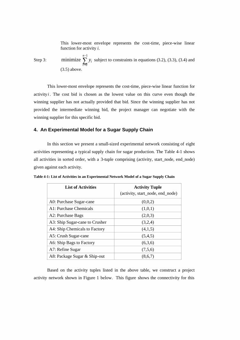
4. An Experimental Model for a Sugar Supply Chain
In this section we present a small-sized experimental network consisting of eight
activities representing a typical supply chain for sugar production. The Table 4-1 shows
all activities in sorted order, with a 3-tuple comprising (activity, start_node, end_node)
given against each activity.
Table 4-1: List of Activities in an Experimental Network Model of a Sugar Supply Chain
List of Activities Activity Tuple (activity, start_node, end_node)
A0: Purchase Sugar-cane (0,0,2) A1: Purchase Chemicals (1,0,1)
A2: Purchase Bags (2,0,3) A3: Ship Sugar-cane to Crusher (3,2,4) A4: Ship Chemicals to Factory (4,1,5)
A5: Crush Sugar-cane (5,4,5) A6: Ship Bags to Factory (6,3,6) A7: Refine Sugar (7,5,6) A8: Package Sugar & Ship-out (8,6,7)
Based on the activity tuples listed in the above table, we construct a project
activity network shown in Figure 1 below. This figure shows the connectivity for this

network in an activity-on-arrow (AOA) network mode and its equivalent activity-on-node
(AON) mode. As already mentioned, in an A-on-A network an activity is represented by
an arc and an event is represented by a node, whereas in an A-on-N network an activity is
represented by a node and an event is represented by an arc. See Kelley (1961) and
Elmaghraby (1977) for a more comprehensive discussion on AOA and AON network
modes. Our experimental implementation uses the AON model of the network.
Figure 1: An Experimental Network Model of a Sugar Supply Chain
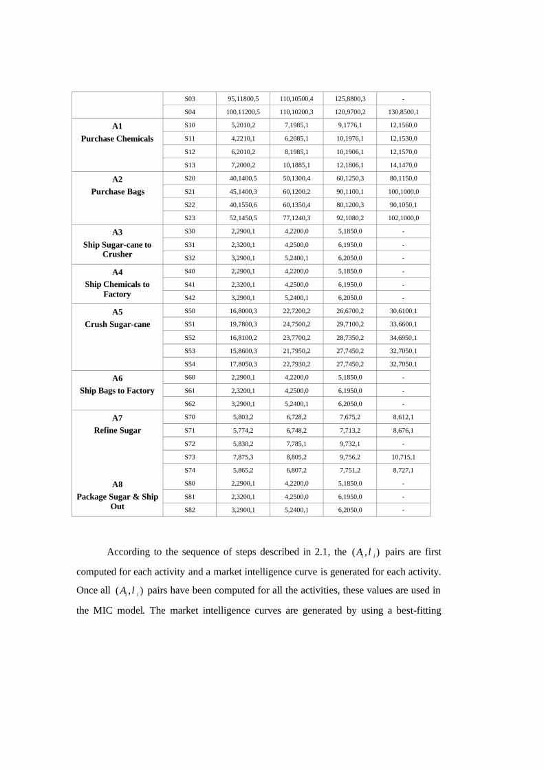
Table 4-2 gives the supplier bids for all activities in this experimental sugar
supply chain (SSC) network. Suppliers provide multiple cost-time bids for each activity
for each activity and each supplier bid is a 3-tuple representing (time, cost, variance).
Individual supplier bids are sorted in ascending order of the time component in the bid.
Table 4-2: Supplier Bids for an Experimental Sugar Supply Chain
Activity Suppliers Bid 1 Bid 2 Bid 3 Bid 4
A0 Purchase Sugar-cane
S00 90,10000,5 100,9000,4 120,8000,3 -
S01 90,11000,6 110,8800,5 120,7700,4 130,6600,2
S02 100,11000,6 110,10000,4 120,8500,3 130,8000,1
S03 95,11800,5 110,10500,4 125,8800,3 -
S04 100,11200,5 110,10200,3 120,9700,2 130,8500,1
A1 Purchase Chemicals
S10 5,2010,2 7,1985,1 9,1776,1 12,1560,0
S11 4,2210,1 6,2085,1 10,1976,1 12,1530,0
S12 6,2010,2 8,1985,1 10,1906,1 12,1570,0
S13 7,2000,2 10,1885,1 12,1806,1 14,1470,0
A2 Purchase Bags
S20 40,1400,5 50,1300,4 60,1250,3 80,1150,0
S21 45,1400,3 60,1200,2 90,1100,1 100,1000,0
S22 40,1550,6 60,1350,4 80,1200,3 90,1050,1
S23 52,1450,5 77,1240,3 92,1080,2 102,1000,0
A3 Ship Sugar-cane to
Crusher
S30 2,2900,1 4,2200,0 5,1850,0 -
S31 2,3200,1 4,2500,0 6,1950,0 -
S32 3,2900,1 5,2400,1 6,2050,0 -
A4 Ship Chemicals to
Factory
S40 2,2900,1 4,2200,0 5,1850,0 -
S41 2,3200,1 4,2500,0 6,1950,0 -
S42 3,2900,1 5,2400,1 6,2050,0 -
A5 Crush Sugar-cane
S50 16,8000,3 22,7200,2 26,6700,2 30,6100,1
S51 19,7800,3 24,7500,2 29,7100,2 33,6600,1
S52 16,8100,2 23,7700,2 28,7350,2 34,6950,1
S53 15,8600,3 21,7950,2 27,7450,2 32,7050,1
S54 17,8050,3 22,7930,2 27,7450,2 32,7050,1
A6 Ship Bags to Factory
S60 2,2900,1 4,2200,0 5,1850,0 -
S61 2,3200,1 4,2500,0 6,1950,0 -
S62 3,2900,1 5,2400,1 6,2050,0 -
A7 Refine Sugar
S70 5,803,2 6,728,2 7,675,2 8,612,1
S71 5,774,2 6,748,2 7,713,2 8,676,1
S72 5,830,2 7,785,1 9,732,1 -
S73 7,875,3 8,805,2 9,756,2 10,715,1
S74 5,865,2 6,807,2 7,751,2 8,727,1
A8 Package Sugar & Ship
Out
S80 2,2900,1 4,2200,0 5,1850,0 -
S81 2,3200,1 4,2500,0 6,1950,0 -
S82 3,2900,1 5,2400,1 6,2050,0 -
According to the sequence of steps described in 2.1, the ( , )i iA λ pairs are first
computed for each activity and a market intelligence curve is generated for each activity.
Once all ( , )i iA λ pairs have been computed for all the activities, these values are used in
the MIC model. The market intelligence curves are generated by using a best-fitting
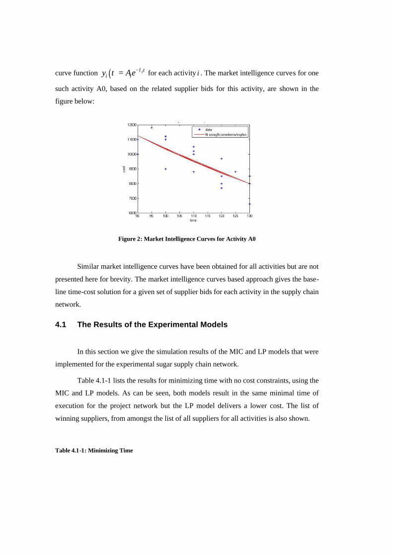
curve function ( ) iti iy t Ae λ−= for each activity i . The market intelligence curves for one
such activity A0, based on the related supplier bids for this activity, are shown in the
figure below:
Figure 2: Market Intelligence Curves for Activity A0
Similar market intelligence curves have been obtained for all activities but are not
presented here for brevity. The market intelligence curves based approach gives the base-
line time-cost solution for a given set of supplier bids for each activity in the supply chain
network.
4.1 The Results of the Experimental Models
In this section we give the simulation results of the MIC and LP models that were
implemented for the experimental sugar supply chain network.
Table 4.1-1 lists the results for minimizing time with no cost constraints, using the
MIC and LP models. As can be seen, both models result in the same minimal time of
execution for the project network but the LP model delivers a lower cost. The list of
winning suppliers, from amongst the list of all suppliers for all activities is also shown.
Table 4.1-1: Minimizing Time
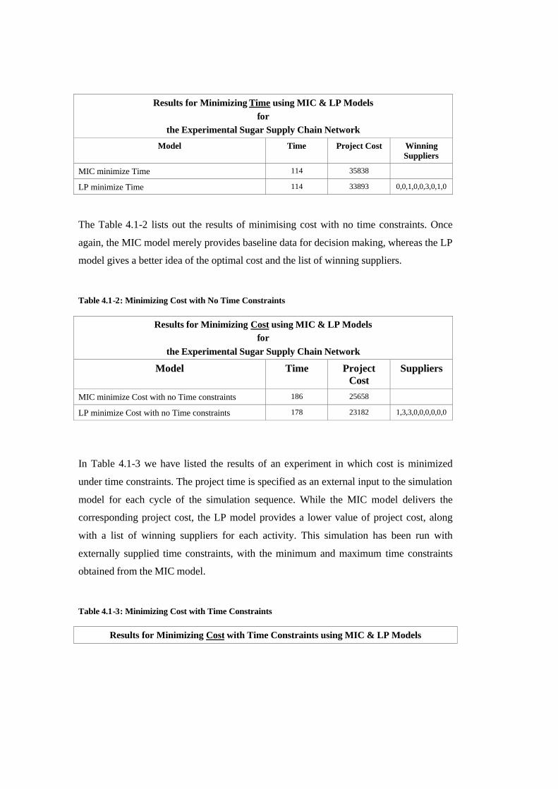
Results for Minimizing Time using MIC & LP Models for
the Experimental Sugar Supply Chain Network
Model Time Project Cost Winning Suppliers
MIC minimize Time 114 35838
LP minimize Time 114 33893 0,0,1,0,0,3,0,1,0
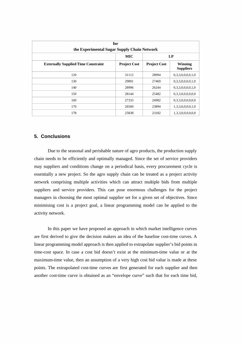
The Table 4.1-2 lists out the results of minimising cost with no time constraints. Once
again, the MIC model merely provides baseline data for decision making, whereas the LP
model gives a better idea of the optimal cost and the list of winning suppliers.
Table 4.1-2: Minimizing Cost with No Time Constraints
Results for Minimizing Cost using MIC & LP Models for
the Experimental Sugar Supply Chain Network
Model Time Project Cost
Suppliers
MIC minimize Cost with no Time constraints 186 25658
LP minimize Cost with no Time constraints 178 23182 1,3,3,0,0,0,0,0,0
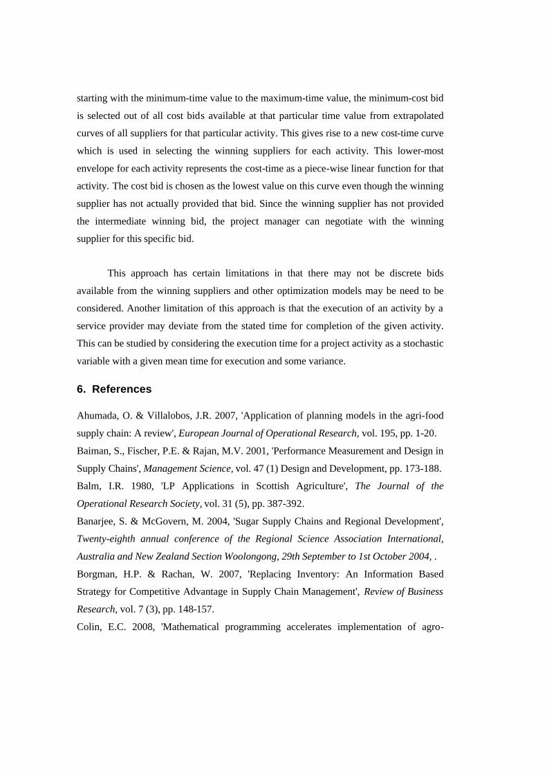
In Table 4.1-3 we have listed the results of an experiment in which cost is minimized
under time constraints. The project time is specified as an external input to the simulation
model for each cycle of the simulation sequence. While the MIC model delivers the
corresponding project cost, the LP model provides a lower value of project cost, along
with a list of winning suppliers for each activity. This simulation has been run with
externally supplied time constraints, with the minimum and maximum time constraints
obtained from the MIC model.
Table 4.1-3: Minimizing Cost with Time Constraints
Results for Minimizing Cost with Time Constraints using MIC & LP Models
for the Experimental Sugar Supply Chain Network
MIC LP
Externally Supplied Time Constraint Project Cost Project Cost Winning Suppliers
120 31112 28994 0,3,3,0,0,0,0,1,0
130 29891 27469 0,3,3,0,0,0,0,1,0
140 28996 26244 0,3,3,0,0,0,0,1,0
150 28144 25482 0,3,3,0,0,0,0,0,0
160 27333 24982 0,3,3,0,0,0,0,0,0
170 26560 23894 1,3,3,0,0,0,0,1,0
178 25838 23182 1,3,3,0,0,0,0,0,0
5. Conclusions
Due to the seasonal and perishable nature of agro products, the production supply
chain needs to be efficiently and optimally managed. Since the set of service providers
may suppliers and conditions change on a periodical basis, every procurement cycle is
essentially a new project. So the agro supply chain can be treated as a project activity
network comprising multiple activities which can attract multiple bids from multiple
suppliers and service providers. This can pose enormous challenges for the project
managers in choosing the most optimal supplier set for a given set of objectives. Since
minimising cost is a project goal, a linear programming model can be applied to the
activity network.
In this paper we have proposed an approach in which market intelligence curves
are first derived to give the decision makers an idea of the baseline cost-time curves. A
linear programming model approach is then applied to extrapolate supplier’s bid points in
time-cost space. In case a cost bid doesn’t exist at the minimum-time value or at the
maximum-time value, then an assumption of a very high cost bid value is made at these
points. The extrapolated cost-time curves are first generated for each supplier and then
another cost-time curve is obtained as an “envelope curve” such that for each time bid,
starting with the minimum-time value to the maximum-time value, the minimum-cost bid
is selected out of all cost bids available at that particular time value from extrapolated
curves of all suppliers for that particular activity. This gives rise to a new cost-time curve
which is used in selecting the winning suppliers for each activity. This lower-most
envelope for each activity represents the cost-time as a piece-wise linear function for that
activity. The cost bid is chosen as the lowest value on this curve even though the winning
supplier has not actually provided that bid. Since the winning supplier has not provided
the intermediate winning bid, the project manager can negotiate with the winning
supplier for this specific bid.
This approach has certain limitations in that there may not be discrete bids
available from the winning suppliers and other optimization models may be need to be
considered. Another limitation of this approach is that the execution of an activity by a
service provider may deviate from the stated time for completion of the given activity.
This can be studied by considering the execution time for a project activity as a stochastic
variable with a given mean time for execution and some variance.
6. References Ahumada, O. & Villalobos, J.R. 2007, 'Application of planning models in the agri-food
supply chain: A review', European Journal of Operational Research, vol. 195, pp. 1-20.
Baiman, S., Fischer, P.E. & Rajan, M.V. 2001, 'Performance Measurement and Design in
Supply Chains', Management Science, vol. 47 (1) Design and Development, pp. 173-188.
Balm, I.R. 1980, 'LP Applications in Scottish Agriculture', The Journal of the
Operational Research Society, vol. 31 (5), pp. 387-392.
Banarjee, S. & McGovern, M. 2004, 'Sugar Supply Chains and Regional Development',
Twenty-eighth annual conference of the Regional Science Association International,
Australia and New Zealand Section Woolongong, 29th September to 1st October 2004, .
Borgman, H.P. & Rachan, W. 2007, 'Replacing Inventory: An Information Based
Strategy for Competitive Advantage in Supply Chain Management', Review of Business
Research, vol. 7 (3), pp. 148-157.
Colin, E.C. 2008, 'Mathematical programming accelerates implementation of agro-
industrial sugarcane complex', European Journal of Operational Research, vol. In press,.
Demeulemeester, E. 1995, 'Minimizing Resource Availability Costs in Time-Limited
Project Networks', Management Science, vol. 41 (10), pp. 1590-1598.
Drexl, A. 1991, 'Scheduling of Project Networks by Job Assignment', Management
Science, vol. 37 (12), pp. 1590-1602.
Elmaghraby, S.E. 1977, Activity Networks: Project Planning and Control by Network
Models, , John Wiley, NY.
Golenko-Ginzburg, D. & Blokh, D. 1997, 'A Generalized Activity Network Model', The
Journal of the Operational Research Society, vol. 48 (4), pp. 391-400.
Golenko-Ginzburg, D. 1989, 'A New Approach to the Activity-Time Distribution in
PERT', The Journal of the Operational Research Society, vol. 40 (4), pp. 389-393.
Gunasekaren, A., Macbeth, D.K. & Lamming, R. 2000, 'Modelling and Analysis of
Supply Chain Management Systems: An Editorial Overview', The Journal of the
Operational Research Society, vol. 51 (10), pp. 1112-1115.
Higgins, A. 2006, 'Scheduling of road vehicles in sugarcane transport: A case study at an
Australian sugar mill', European Journal of Operational Research, vol. 170, pp. 987-
1000.
Higgins, A., Beashel, G. & Harrison, A. 2006, 'Scheduling of Brand Production and
Shipping within a Sugar Supply Chain', Journal of the Operational Research Society, vol.
57 (5), pp. 490-498.
Higgins, A.J. & Laredo, L.A. 2006, 'Improving harvesting and transport planning within
a sugar value chain', Journal of the Operational Research Society, vol. 57, pp. 367-376.
Jiao, Z., Higgins, A.J. & Prestwidge, D.B. 2005, 'An integrated statistical and
optimisation approach to increasing sugar production within a mill region', Computers
and Electronics in Agriculture, vol. 48, pp. 170-181.
Kelley, J.E. & Walker, M.R. (1959). Critical-path planning and scheduling. IRE-AIEE-
ACM '59 (Eastern): Papers presented at the December 1-3, 1959, eastern joint IRE-
AIEE-ACM computer conference (pp. 160-173). New York, NY, USA:ACM.
Kelley, J.E. 1961, Critical-Path Planning and Scheduling: Mathematical Basis, .
Le Gal, P., Lyne, P.W.L. & Soler, L. 2008, 'Impact of sugarcane supply scheduling on
mill sugar production: A South African case study', Agricultural Systems, vol. 96, pp. 64-

74.
Lejars, C., Le Gal, P. & Auzoux, S. 2008, 'A decision support approach for cane supply
management within a sugar mill area', Computers And Electronics In Agriculture, vol.
60, pp. 239-249.
Parikh, S.C. & Jewell, W.S. 1965, 'Decomposition of Project Networks', Management
Science, vol. 11 (3) Series A, Sciences, pp. 444-459.
Sargent, E.D. 1980, 'The Impact of Operational Research on Agriculture', The Journal of
the Operational Research Society, vol. 31 (6), pp. 477-483.