Optimal Monetary Policy, Exchange Rate

Misalignments and Incomplete Financial Markets∗

Ozge Senay†and Alan Sutherland‡

February 2017

Abstract

Recent literature on monetary policy in open economies shows that, when in-

ternational financial trade is restricted to a single non-contingent bond, there are

significant internal and external trade-offs that prevent optimal policy from simul-

taneously closing all welfare gaps. This implies that optimal policy deviates from

inflation targeting in order to offset real exchange rate misalignments. These simple

models are, however, not good representations of modern financial markets. This

paper therefore develops a more general and realistic two-country model of incom-

plete markets, where, in the presence of a wide range of stochastic shocks, there

is international trade in nominal bonds and equities. The analysis shows that, as

in the recent literature, optimal policy deviates from inflation targeting in order to

offset exchange rate misalignments, but the welfare benefits of optimal policy rela-

tive to inflation targeting are quantitatively smaller than found in simpler models of

financial incompleteness. It is nevertheless found that optimal policy implies quan-

titatively significant stabilisation of the real exchange rate gap and trade balance

gap compared to inflation targeting.

Keywords: Optimal monetary policy, Financial market structure, Country Port-

folios

JEL: E52, E58, F41

∗We are grateful to Kemal Ozhan and Oliver de Groot for helpful comments on an earlier draft of

this paper. This research is supported by ESRC Award Number ES/I024174/1.†University of St Andrews. Address: School of Economics and Finance, University of St Andrews, St

Andrews, KY16 9AL, UK. E-mail: os12@st-and.ac.uk Tel: +44 1334 462422.‡CEPR and University of St Andrews. Address: School of Economics and Finance, University of St

Andrews, St Andrews, KY16 9AL, UK. E-mail: ajs10@st-and.ac.uk Tel: +44 1334 462446.

1 Introduction

To what extent should the design of monetary policy rules explicitly account for open

economy factors such as current account imbalances or exchange rate misalignments?

The early literature on optimal monetary policy in open economies gives the clear answer

that open economy factors need have no explicit role in the design of monetary policy

rules. For instance, the work of Clarida et al (2002), Gali and Monacelli (2005) and

Benigno and Benigno (2003) shows that monetary policy should focus on targeting the

rate of inflation of producer prices. These authors demonstrate that a policy of inflation

targeting is sufficient to close all internal and external welfare gaps. So, for instance a

policy of inflation targeting would imply a rise in the policy interest rate in response to

a negative TFP shock and thus would close the gap between actual and potential output

and also close the gap between the actual and welfare optimal real exchange rate and trade

balance. There is therefore no trade-off between internal and external policy objectives.

This early literature is in effect a direct extension to an open economy setting of the basic

closed economy results of Woodford (2003) and Benigno and Woodford (2005). The only

difference between the closed and open economy results is in the choice of price index for

the inflation target - consumer prices for a closed economy and producer prices for an

open economy.

This early open economy literature, however, focused on models where international

financial markets are complete. Households can therefore fully hedge against country

specific income shocks. More recent literature has begun to analyse monetary policy in

open economy models where financial markets are incomplete. For instance, Corsetti

et al (2010, 2011) analyse monetary policy in a context where international financial

trade is absent or is restricted to a single non-contingent bond. They show that, in

contrast to the previous literature, when international financial markets are incomplete

there are significant internal and external trade-offs that prevent optimal policy from

simultaneously closing all welfare relevant gaps.1

The basic intuition for the Corsetti et al (2010, 2011) results is simple to explain.

A policy of producer price inflation targeting reproduces the flexible price outcome and

1Corsetti et al (2010, 2011) focus on optimal monetary policy in a symmetric two-country world.

Benigno (2009) analyses an asymmetric world with incomplete financial markets and shows how optimal

monetary policy differs between net-debtor and net-creditor countries. De Paoli (2010) analyses monetary

policy for a small open economy and shows how optimal policy depends on the degree of financial

integration.

1

therefore eliminates the welfare costs associated with staggered price setting. But the

flexible price equilibrium is not fully optimal because international financial markets are

imperfect and thus cross-country income risks are not optimally shared. A corollary of this

is that the real exchange rate and trade balance will deviate from their first best outcomes.

Corsetti et al (2010, 2011) show that optimal policy deviates from inflation targeting and

takes account of external welfare gaps and acts to offset "exchange rate misalignments."

They argue that external factors are particularly important in two cases. The first is

when the elasticity of substitution between goods produced in different countries (i.e. the

trade elasticity) is low. The second is when firms adopt local currency pricing (i.e. they

set prices in the currency of the buyer).

The results in Corsetti et al (2010, 2011) clearly point to a potentially important

deviation from the standard policy prescription of inflation targeting. There is however

a significant limitation to Corsetti et al ’s work. In Corsetti et al (2010) the analysis of

imperfect international financial markets is restricted to a model with financial autarky,

while in Corsetti et al (2011) the analysis of imperfect financial markets is represented by

a single bond economy. These structures provide important insights into the implications

of imperfect financial trade but they are obviously not a good representation of modern

international financial markets.

The main objective of the current paper is to analyse more general models of imperfect

international financial trade than those considered in Corsetti et al (2010, 2011). Our

model is more general in a number of dimensions. Firstly, we examine a more general

financial market structure where agents can trade in both equities and bonds. Secondly,

we allow for more sources of stochastic shocks. And thirdly, in an extended version of

the model, we incorporate variable real capital. By allowing for trade in a wider range

of financial assets we provide more scope for hedging than in the Corsetti et al (2010,

2011) structure. By including more stochastic shocks we ensure that, despite the presence

of more assets, financial markets are still not complete. Our model is therefore a more

realistic framework for analysing the implications of imperfect financial markets for the

design of optimal monetary policy rules. Our objective is to test whether the Corsetti

et al (2010, 2011) results continue to hold in this more realistic structure and, if they

do, what is the quantitative significance of financial market incompleteness in terms of

departures from inflation stabilisation.

Because our model allows for international trade in nominal bonds and equities it is

necessary to compute equilibrium gross portfolios. The size and composition of these

2

portfolios will depend on the structure and stochastic environment of the model, includ-

ing the properties of the monetary rule. There is therefore an interaction between policy

choice and portfolio choice. Equilibrium portfolios are computed using techniques devel-

oped in recent literature (see Devereux and Sutherland (2010, 2011a) and Tille and van

Wincoop (2010)). The combining of these techniques with the analysis of optimal policy

is an important innovation of this paper.2

After describing our model our analysis focuses on a comparison between optimal

policy and a policy of strict (producer price) inflation targeting. This comparison allows

us to judge the extent to which optimal policy deviates from an internal objective (i.e.

inflation stability) in order to achieve open economy objectives such as correcting real

exchange rate misalignments. Our results show that the welfare gain of optimal policy

relative to strict inflation targeting is quite small. This is true for a wide range of

parameter values (including the cases emphasised by Corsetti et al (2010, 2011)). It

therefore appears that the extra hedging possibilities offered by the wider range of assets

incorporated in our model tends to reduce the trade-off between internal and external

policy objectives that is highlighted by Corsetti et al (2010, 2011). However, our results

show that, despite the small welfare gains generated by optimal policy, it continues to be

the case that optimal policy tends to reduce the volatility of the real exchange rate and

the trade balance (as measured against their first-best values). Thus optimal policy does

tend to deviate from strict inflation targeting in order to correct measures of external

misalignment.

The paper proceeds as follows. The model is presented in Section 2. Our definition

of welfare and the characterisation of monetary policy is described in Section 3 and our

methodology for deriving optimal policy rules in the presence of endogenous portfolio

choice is described in Section 4. The main results of the paper are presented in Section 5

and the results from an extended version of the model are described in Section 6. Section

7 concludes the paper.

2Devereux and Sutherland (2008) consider a simple case where optimal monetary policy can be

analysed alongside endogenous portfolio choice. However, in that case asset trade is restricted to two

nominal bonds and only a limited range of exogenous shocks is considered. They show that, in these

special circumstances, strict inflation targeting reproduces the full risk sharing outcome, so there is no

trade-off between internal and external policy objectives.

3

2 The Model

We analyse a model of two countries with multiple sources of shocks. The model shares

many of the same basic features of the closed economy models developed by Christiano

et al (2005) and Smets and Wouters (2003). It is based on the open economy model

developed in Devereux et al (2014).

Households consume a basket of home and foreign produced final goods. Final goods

are produced by monopolistically competitive firms which use intermediate goods as their

only input. Final goods prices are subject to Calvo-style contracts. Intermediate goods

are produced by perfectly competitive firms using labour and real capital as inputs.

Intermediate goods prices are perfectly flexible. In the benchmark version of the model

the capital stock is fixed. In an extended version of the model we allow for variable capital

stocks which are subject to adjustment costs. Households supply homogeneous labour to

perfectly competitive firms producing intermediate goods. All profits from firms in the

intermediate and final goods sectors are paid to holders of equity shares.

We allow for international trade in equities and nominal bonds. Home and foreign

equities represent claims on aggregate firm profits of each country, and home and foreign

nominal bonds are denominated in the currency of each country.

The following sections describe the home country in detail. The foreign country is

identical. An asterisk indicates a foreign variable or a price in foreign currency.

2.1 Households

Household in the home country maximizes a utility function of the form

=

∞P=0

(Ψ+

1−+ ()

1− −∆+

1++ ()

1 +

)(1)

where 0 0, () is the consumption of household , () is labour supply,

is the discount factor and Ψ and ∆ are stochastic preference shocks which affect

consumption and labour supply respectively. We assume ∆ = ∆ exp(∆) where ∆ =

∆∆−1 + ∆ 0 ≤ ∆ 1 and ∆ is a zero-mean normally distributed i.i.d. shock with

[∆] = 2∆ and Ψ = Ψ exp(Ψ) where Ψ = ΨΨ−1 + Ψ 0 ≤ Ψ 1 and Ψ is a

zero-mean normally distributed i.i.d. shock with [Ψ] = 2Ψ

Taste shocks in the form of Ψ are emphasised by Corsetti et al (2010, 2011) because

they create a strong role for current account dynamics and thus potentially create a strong

welfare trade-off for monetary policy when financial markets are incomplete.

4

The discount factor, is endogenous and is determined as follows

+1 =

µ

¶− 0 = 1 (2)

where 0 , 0 1, is aggregate home consumption and is a constant.3

We define to be a consumption basket which aggregates home and foreign goods

according to:

=h1

−1

+ (1− )1

−1

i −1

(3)

where and are baskets of individual home and foreign produced goods. The

elasticity of substitution across individual goods within these baskets is 1. The

parameter in (3) is the elasticity of substitution between home and foreign goods. The

parameter measures the importance of consumption of the home good in preferences.

For 12, we have ‘home bias’ in preferences.

The price index associated with the consumption basket is

=£ 1−

+ (1− ) 1−

¤ 11− (4)

where is the price index of home goods for home consumers and is the price

index of foreign goods for home consumers. The corresponding price indices for foreign

consumers are and

The flow budget constraint of the home country household is

+ = + Π − +

P=1

−1 (5)

where denotes home country net external assets in terms of the home consumption

basket, is the home nominal wage, Π is profits of all home firms and is lump-sum

taxes imposed on households. The final term represents the total return on the home

country portfolio where −1 represents the real external holdings of asset (defined

in terms of the home consumption basket) purchased at the end of period − 1 and represents the gross real return on asset . In our analysis, we allow for trade in

= 4 assets; home and foreign equity and home and foreign nominal bonds. Note that

=P

=1 .

Nominal bonds are assumed to be perpetuities, so for instance, home nominal bonds

represent a claim on a unit of home currency in each period into the infinite future. The

3Following Schmitt-Grohe and Uribe (2003), is assumed to be taken as exogenous by individual

decision makers. The impact of individual consumption on the discount factor is therefore not internal-

ized.

5

real price of the home bond is denoted The gross real rate of return on a home

bond is thus +1 = (1+1 + +1) For the foreign nominal bond, the real

return on foreign bonds, in terms of home consumption, is ∗+1 = (+1)(1∗+1 +

∗+1)∗, where =

∗ is the real exchange rate (where is the price of the

foreign currency in terms of the home currency).

Home equities represent a claim on aggregate profits of all firms in the home final

and intermediate sectors. The real payoff to a unit of the home equity purchased in

period is defined to be Π+1 ++1, where +1 is the real price of home equity and

Π+1 is real aggregate profits. Thus the gross real rate of return on the home equity is

+1 = (Π+1 + +1).

2.2 Firms

Within each country firms are divided between final and intermediate sectors. Interme-

diate goods firms use labour and real capital. There is a unit mass of firms in both the

final and intermediate levels.

2.2.1 Final goods

Each firm in the final goods sector produces a single differentiated product. Sticky prices

are modelled in the form of Calvo (1983) style contracts with a probability of re-setting

price given by 1 − . We consider both producer currency pricing (PCP) and local

currency pricing (LCP).

If firms use the discount factor Ω to evaluate future profits, then, in the PCP case,

firm chooses its prices for home and foreign buyers, () and () in home

currency to maximize

∞P=0

Ω+

½+()

[()− +]

+

+ +()[()− +]

+

¾(6)

where () is the demand for home good from home buyers and () is the

demand for home good from foreign buyers and is the price of the intermediate good.

In the LCP case firm chooses () in home currency and ∗() in foreign

currency to maximize (6) where () is replaced by ∗()+ where is the

nominal exchange rate (defined as the foreign currency in terms of the home currency).

Monopoly power in the final goods sector implies that final goods prices are subject to

a mark-up given by = (−1) The mark-up is assumed to be subject to stochastic

6

shocks such that = exp() where = −1 + , 0 ≤ 1 and is a

zero-mean normally distributed i.i.d. shock with [] = 2.

2.2.2 Intermediate goods

The representative firm in the intermediate goods sector combines labour, , and capital,

, to produce output using a standard Cobb-Douglas technology, = 1−−1

We assume that total factor productivity, is determined as follows

= −

where

= −1 + + = −1 +

where and and are zero mean normally distributed i.i.d. shocks. This

structure captures the concept of "news shocks" as in Beaudry and Portier (2006). News

shocks are emphasised by Corsetti et al (2010, 2011) because news shocks create a strong

role for current account dynamics and therefore a potentially strong welfare trade-off

between internal and external policy objectives when financial markets are incomplete.

In the benchmark version of the mode we assume that the stock of real capital is fixed

at .

The representative firm chooses to maximize the real discounted value of dividends,

given by

∞P=0

Ω+

∙+

+

+ − +

+

+

¸subject to the production function where is the price of intermediate goods. Ω is

assumed to be the stochastic discount factor of shareholders of the firm.

2.3 Government

Total government expenditure is assumed to be exogenous and subject to stochastic

shocks. In particular we assume that = exp() is government spending where

= −1 + , 0 ≤ 1 and is a zero-mean normally distributed i.i.d. shock

with [] = 2.

All government spending is financed via lump sum taxes on households, and

firms, The budget constraint is = + where it is assumed that

= (1− ) and = where is a fixed parameter which determines

the share of profit taxes in the overall tax take. is the price index of government

7

purchased goods. It is assumed that government spending is on domestically produced

goods so =

As with taste and news shocks, transitory government spending shocks of the type

assumed here create a potentially strong role for current account dynamics and therefore a

potentially strong welfare trade-off between internal and external policy objectives when

financial markets are incomplete.

2.4 Equilibrium

Home demand for home final goods is

=

µ

¶− (7)

Each home country firm in the final goods sector faces demand for its good from the

home and foreign countries. Equilibrium in the market for good in the home country

final goods sector implies () = () + () where

() =

µ()

¶−[ +] () =

Ã∗()

∗

!−∗

(8)

where ∗ is the foreign demand for home goods (defined analogously to (7)).

Aggregate GDP for the home economy is given by

=

[ +] +

∗

∗

where is the GDP deflator, which we define as follows

= [(1− ) + ] + (1− )(1− )∗

where is the steady-state share of government spending in GDP.

Equilibrium in the labour market implies =

Total after-tax dividends aggregated across all intermediate and final goods firms are

given by

Π =

−

−

Home equities represent claims on Π (into the infinite future).

It is useful to define the terms of trade as follows

=

∗

8

3 Monetary Policy and Welfare

The particular welfare measure on which we focus is the unconditional expectation of

aggregate period utility. For the home economy this is defined as follows

=

½Ψ1−

1− −∆

1+

1 +

¾(9)

where time subscripts are omitted to indicate that this is a measure of unconditional

expectation. Damjanovic et al (2008) argue that unconditionally expected utility provides

a useful alternative to Woodford’s (2003) ‘timeless perspective’ when analysing optimal

policy problems. For the purposes of this paper, unconditional expected utility provides

a simple and convenient way to compute welfare in a context where portfolio allocation

is endogenous. The next section provides a more detailed discussion of the complications

that arise in the simultaneous computation of welfare and equilibrium portfolios.

In common with Corsetti et al (2010, 2011) and much of the previous literature we

focus on co-operative policy in the sense that policy rules for each country are simulta-

neously chosen to maximise global welfare, i.e. the sum of the home and foreign welfare

measures.

We model monetary policy in the form of a ‘targeting rule’.4 In general the optimal

targeting rule is model dependent. Corsetti et al (2010, 2011) show that the optimal

targeting rule for a model similar to ours includes measures of inflation and a number of

welfare gaps. Because of the complicated interaction between policy and portfolio choice

we do not derive the fully optimal policy rule for our model. Instead we use the form of

the optimal rule derived by Corsetti et al (2010, 2011) as an approximation for optimal

policy in our model.

For the home economy, the targeting rule derived by Corsetti et al (2010, 2011) has

the following form

( − −1) + (1− )( − −1) + ( − −1)

+( − −1) + D(D −D−1) + L(L − L−1) = 0 (10)

4As argued by Woodford (2003), a ‘targeting rule’ is a convenient way to capture the welfare trade-offs

faced by policy makers. It allows policy to be specified in terms of an optimal equilibrium relationship

between various welfare ‘gaps’. Once policy is specified in this way there is no need explicitly to model

policy in terms of the optimal setting of a policy instrument (such as the nominal interest rate). However,

an implied optimal rule for the policy instrument can easily be derived once the optimal equilibrium has

been derived.

9

where a hat over a variable represents its log deviation from the non-stochastic steady

state and , , D and L are defined as follows

= −

= −

D = −³ − ∗

´+ − (Ψ− Ψ∗)

L = − − ∗

where the superscript indicates the first best value of a variable. Thus is a measure

of the output gap and is a measure of the terms of trade gap. The variables D and

L also measure deviations from first best outcomes. As will be explained in more detail

below, D is a measure of the deviation from full risk sharing and L is a measure of thedeviation from the law of one price. There is an analogous targeting rule for the foreign

economy.

The targeting rule in (10) contains six terms. The first two terms represent a weighted

average of producer price (PPI) and consumer price (CPI) inflation. The central role

of inflation stabilisation in optimal policy in New Keynesian models is a well-known

consequence of staggered price setting. In essence, staggered price setting implies that

inflation causes distortions in relative prices between goods. Inflation is thus (other

things equal) welfare reducing. It is also well-known that, in the presence of PCP, the

welfare-relevant measure of inflation is PPI inflation. This is captured by the first term in

(10). Engel (2011) shows that, for certain parameter combinations, in the LCP case the

welfare-relevant measure of inflation is CPI inflation. Corsetti et al (2010, 2011) show

that, for general parameter combinations, in the LCP case the welfare-relevant measure

of inflation is effectively a weighted average of PPI and CPI inflation. This general case

is therefore captured by the first two terms in (10).

The third term in (10) measures the welfare-relevant output gap. Again the role of

the output gap in optimal targeting rules in New Keynesian models is well-known and

needs no further explanation.

The fourth term in the targeting rule measures the welfare-relevant terms-of-trade

gap. As Corsetti et al (2010, 2011) explain in detail, in an open economy, because

there are different baskets of goods produced in different countries, shocks may have

distortionary effects on the relative price of these different baskets. These distortions are

welfare reducing in the same way as the within-country price distortions generated by

10

inflation are welfare reducing. The terms of trade gap therefore plays the same role in

the monetary policy rule as the CPI and PPI inflation terms.

The fifth term in the targeting rule is referred to by Corsetti et al (2010, 2011) as

a measure of "demand imbalances". It measures deviations from full risk sharing. This

captures the welfare reducing effects of incomplete financial markets. To understand this

term note that, if a complete set of financial instruments were available for international

trade, equilibrium in financial markets would imply that the ratio of marginal utilities

across countries would equal the relative price of consumption baskets, i.e.

Ψ∗∗−

Ψ−

=

or in terms of log-deviations

−(Ψ− Ψ∗)− ³ − ∗

´+ = 0

This is the well-known risk sharing condition that is standard in open-economy models

with complete financial markets. It is thus clear that D in (10) is a measure of deviationsfrom full risk sharing. And it is clear that this term in the monetary policy rule captures

the extent to which monetary policy is adjusted in order to achieve greater risk sharing.

The final term in the targeting rule captures the welfare reducing effects of deviations

from the law of one price. Such deviations are a direct consequence of (and only arise

from) local currency pricing. In a similar way to the price distortions caused by stag-

gered pricing, deviations from the law of one price are a form of price distortion which

potentially requires a monetary policy response.

The six terms in the policy rule capture a range of potential welfare trade-offs that

feature in the optimal setting of monetary policy. Internal (i.e. with-in country) trade-

offs are captured by the inflation terms and the output gap. External (i.e. open economy)

trade-offs are captured by the terms of trade, demand imbalances and law-of-one-price

terms in the policy rule. The object of the analysis presented below is to determine the

optimal values of the coefficients of the policy rule and thus to determine the role of

external versus internal trade-offs in the optimal setting of monetary policy.

Note that policy rule (10) contains CPI and PPI inflation targeting as special cases.

CPI inflation targeting is given by = = = D = L = 0 and PPI inflation

targeting is given by = 1, = = D = L = 0

11

4 Model Solution, Country Portfolios and Policy Op-

timisation

Our objective in this paper is to analyse optimal monetary policy in the above specified

model. The key distinguishing feature of the above model, that sets it apart from much of

the existing literature on optimal monetary policy in open economies, is that it allows for

international trade in multiple assets. Recently developed solution techniques (Devereux

and Sutherland, 2011a) make it possible to solve for equilibrium portfolio allocation in

models of this type and there is now an active literature applying these techniques to a

range of positive questions. The purpose of our paper is to apply these techniques to the

analysis of optimal monetary policy in the presence of endogenous portfolio choice.

Combining the analysis of optimal policy and endogenous portfolio choice presents

some new technical challenges. These challenges arise because there is an interaction

between policy choices and portfolio choice. Portfolio choices depend on the stochastic

properties of income and the hedging properties of available assets. Monetary policy af-

fects the stochastic behaviour of income and the hedging properties of assets and therefore

affects optimal portfolio choice. In turn, the equilibrium portfolio affects consumption

and labour supply choices and thus affects macroeconomic outcomes and welfare. Thus,

in addition to the standard routes via which policy affects the macro economy, the op-

timal choice of monetary policy must take account of the welfare effects of policy that

occur via the effects of policy on portfolio allocation.

Our solution approach follows the recent portfolio literature based on Devereux and

Sutherland (2011a) in computing equilibrium portfolios using a second order approxima-

tion to the portfolio selection equations for the home and foreign country in conjunction

with a first order approximation to the home and foreign budget constraints and the vec-

tor of excess returns. The innovation in this paper is to combine this portfolio solution

approach with an analysis of optimal monetary policy.

As already explained, we model monetary policy as targeting rule (10). We optimise

the choice of coefficients in the targeting rule by means of a grid search algorithm. Each

grid point represents a different setting of the coefficients of the targeting rule and for

each grid point there is an equilibrium portfolio allocation and a corresponding general

macroeconomic equilibrium and level of welfare. We use the Devereux and Sutherland

portfolio solution approach to evaluate the equilibrium portfolio at each grid point. This

equilibrium portfolio is then used to compute macroeconomic equilibrium and a second

12

order approximation of welfare at each grid point.

To be specific, our policy optimisation problem involves a grid search across the five

coefficients of the policy rule in (10), i.e. D and L, in order to identify the

parameter combination which maximises the unconditional expectation of period welfare

(as defined in (120)).5

It should be noted that this methodology does not compute fully optimal policy

because fully optimal policy may involve more inertia than is embodied in the above

specified targeting rule (as is shown in Corsetti et al (2010, 2011) in some cases). Our

optimal rule is therefore the optimal rule within the restricted class of rules defined by

(10). The focus on a non-inertial targeting rule is a convenient simplification given the

extra complications and computational burden arising from the endogenous determination

of equilibrium portfolios.

5 Comparison of Optimal Monetary Policy and In-

flation Targeting

5.1 Benchmark parameter values

The benchmark parameter values used in the following analysis are listed in Table 1.

Many of these parameter values are taken directly from Corsetti et al (2010, 2011). The

values of (the elasticity of substitution between individual final goods) and (the

Cobb-Douglas coefficient on labour in the production function of intermediate goods) are

chosen to yield a steady state monopoly mark-up of 11% and share of capital in output

of 033. The implied steady state share of dividends in GDP is approximately 015. The

Calvo parameter for price setting, is chosen to imply an average period between price

changes of 4 quarters. The values of (inverse labour elasticity) and (risk aversion) are

consistent with the estimates of Smets and Wouters (2003, 2005, 2007). The steady state

share of government spending in GDP, , is set at 0.2 and the share of dividend taxes

in total taxes, is set at 0.15 (which is approximately the same as the assumed steady

state share of dividends in total income). The parameters of the endogenous discount

factor, and are chosen to yield a steady state rate of return of approximately 4%.

5Given that the model is symmetric, the foreign country has a similarly defined targeting rule and the

coefficients of that rule are assumed to be identical to the coefficients of the home rule, with appropriate

changes of sign.

13

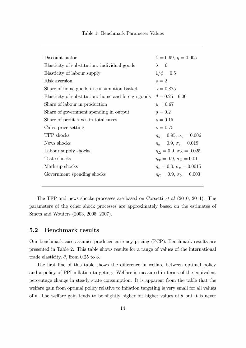
Table 1: Benchmark Parameter Values

Discount factor = 099 = 0005

Elasticity of substitution: individual goods = 6

Elasticity of labour supply 1 = 05

Risk aversion = 2

Share of home goods in consumption basket = 0875

Elasticity of substitution: home and foreign goods = 025 - 600

Share of labour in production = 067

Share of government spending in output = 02

Share of profit taxes in total taxes = 015

Calvo price setting = 075

TFP shocks = 095 = 0006

News shocks = 09 = 0019

Labour supply shocks ∆ = 09 ∆ = 0025

Taste shocks Ψ = 09 Ψ = 001

Mark-up shocks = 00 = 00015

Government spending shocks = 09 = 0003

The TFP and news shocks processes are based on Corsetti et al (2010, 2011). The

parameters of the other shock processes are approximately based on the estimates of

Smets and Wouters (2003, 2005, 2007).

5.2 Benchmark results

Our benchmark case assumes producer currency pricing (PCP). Benchmark results are

presented in Table 2. This table shows results for a range of values of the international

trade elasticity, from 0.25 to 3.

The first line of this table shows the difference in welfare between optimal policy

and a policy of PPI inflation targeting. Welfare is measured in terms of the equivalent

percentage change in steady state consumption. It is apparent from the table that the

welfare gain from optimal policy relative to inflation targeting is very small for all values

of The welfare gain tends to be slightly higher for higher values of but it is never

14

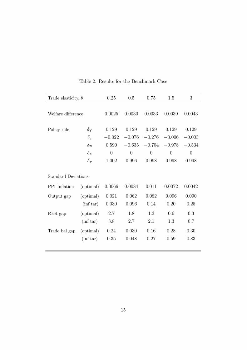
Table 2: Results for the Benchmark Case

Trade elasticity, 025 05 075 15 3

Welfare difference 00025 00030 00033 00039 00043

Policy rule 0129 0129 0129 0129 0129

−0022 −0076 −0276 −0006 −0003D 0590 −0635 −0704 −0978 −0534L 0 0 0 0 0

1002 0996 0998 0998 0998

Standard Deviations

PPI Inflation (optimal) 00066 00084 0011 00072 00042

Output gap (optimal) 0021 0062 0082 0096 0090

(inf tar) 0030 0096 014 020 025

RER gap (optimal) 27 18 13 06 03

(inf tar) 38 27 21 13 07

Trade bal gap (optimal) 024 0030 016 028 030

(inf tar) 035 0048 027 059 083

15

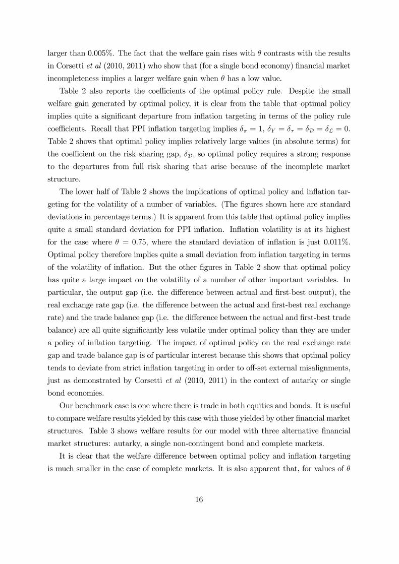
larger than 0.005%. The fact that the welfare gain rises with contrasts with the results

in Corsetti et al (2010, 2011) who show that (for a single bond economy) financial market

incompleteness implies a larger welfare gain when has a low value.

Table 2 also reports the coefficients of the optimal policy rule. Despite the small

welfare gain generated by optimal policy, it is clear from the table that optimal policy

implies quite a significant departure from inflation targeting in terms of the policy rule

coefficients. Recall that PPI inflation targeting implies = 1, = = D = L = 0.

Table 2 shows that optimal policy implies relatively large values (in absolute terms) for

the coefficient on the risk sharing gap, D so optimal policy requires a strong response

to the departures from full risk sharing that arise because of the incomplete market

structure.

The lower half of Table 2 shows the implications of optimal policy and inflation tar-

geting for the volatility of a number of variables. (The figures shown here are standard

deviations in percentage terms.) It is apparent from this table that optimal policy implies

quite a small standard deviation for PPI inflation. Inflation volatility is at its highest

for the case where = 075 where the standard deviation of inflation is just 0.011%.

Optimal policy therefore implies quite a small deviation from inflation targeting in terms

of the volatility of inflation. But the other figures in Table 2 show that optimal policy

has quite a large impact on the volatility of a number of other important variables. In

particular, the output gap (i.e. the difference between actual and first-best output), the

real exchange rate gap (i.e. the difference between the actual and first-best real exchange

rate) and the trade balance gap (i.e. the difference between the actual and first-best trade

balance) are all quite significantly less volatile under optimal policy than they are under

a policy of inflation targeting. The impact of optimal policy on the real exchange rate

gap and trade balance gap is of particular interest because this shows that optimal policy

tends to deviate from strict inflation targeting in order to off-set external misalignments,

just as demonstrated by Corsetti et al (2010, 2011) in the context of autarky or single

bond economies.

Our benchmark case is one where there is trade in both equities and bonds. It is useful

to compare welfare results yielded by this case with those yielded by other financial market

structures. Table 3 shows welfare results for our model with three alternative financial

market structures: autarky, a single non-contingent bond and complete markets.

It is clear that the welfare difference between optimal policy and inflation targeting

is much smaller in the case of complete markets. It is also apparent that, for values of

16

Table 3: Welfare and alternative financial market structures (PCP)

Trade elasticity, 025 05 075 15 3

Bonds and equities 00025 00030 00033 00039 00043

Single bond 00039 032 72× 10−6 29× 10−5 76× 10−5Complete markets 57× 10−6 62× 10−6 66× 10−6 75× 10−6 84× 10−6Autarky 89× 10−4 010 40× 10−5 11× 10−5 74× 10−6

close to 0.5, the welfare gain from optimal policy is much higher in the autarky and single-

bond cases. For instance, in the single bond case at = 05 the welfare difference rises

to 0.32% of steady state consumption. These last results thus replicate (in qualitative

terms) the Corsetti et al (2010, 2011) results which emphasise that the welfare gain from

optimal policy can be quite significant for low values of . Notice, however, that, in

contrast to the arguments of Corsetti et al (2010, 2011), the impact of on the welfare

gain appears to be non-monotonic. So, for very low values of (i.e. = 025) the welfare

gain of optimal policy is very small, even in the autarky and single bond cases.

5.3 Local currency pricing

Corsetti et al (2010, 2011) argue that financial market incompleteness is likely to be par-

ticularly important in the case of local currency pricing (LCP). Table 4 therefore reports

results for this case where we now compare optimal policy to CPI inflation targeting.

The results reported in Table 4 for the LCP case appear to be very similar to those

shown in Table 2 for the PCP case. As in the PCP case the welfare gains for optimal

policy relative to inflation targeting are small. In no case is the welfare gain more than

0.005% of steady state consumption. It therefore appears that, in contrast to the results

reported by Corsetti et al (2010, 2011), there is no significant difference between the LCP

and PCP cases in terms of welfare.

Despite the small welfare gain from optimal policy, Table 4 shows that, as with the

PCP case, optimal policy does imply quite significant departures from inflation targeting

in terms of the coefficients of the policy rule. Recall that CPI inflation targeting implies

= = = D = L = 0 It is apparent from Table 4 that optimal policy requires

quite significant policy responses to departures from risk sharing (as indicated by the

17

Table 4: Local Currency Pricing

Trade elasticity, 025 05 075 15 3

Welfare difference 00027 00030 00032 00034 00037

Policy rule 0123 2058 0186 0136 0133

−1190 −0198 −0312 −0294 −0202D 0252 −1862 −2170 −1039 −1600L 2364 0393 0528 0444 0263

0302 0334 0353 0330 0336

Standard Deviations

CPI Inflation (optimal) 00054 00048 00043 00029 00020

Output gap (optimal) 00039 011 015 021 024

(inf tar) 00078 015 020 028 033

RER gap (optimal) 28 20 17 14 14

(inf tar) 37 27 22 16 14

Trade bal gap (optimal) 072 042 029 031 046

(inf tar) 072 039 033 056 085

18

Table 5: Welfare and alternative financial market structures (LCP)

Trade elasticity, 025 05 075 15 3

Bonds and equities 00027 00030 00032 00034 00037

Single bond 00062 035 68× 10−4 23× 10−4 10× 10−4Complete markets 12× 10−3 92× 10−4 72× 10−4 39× 10−4 15× 10−4Autarky − − 10× 10−3 97× 10−5 14× 10−4

non-zero value for D), the terms of trade gap (as indicated by the non-zero value for )

and departures from the law of one price (as indicated by the non-zero value for L).

The lower half of Table 4 shows that, as with the PCP case, optimal policy appears to

deliver quite significant stabilisation of the real exchange rate and trade balance relative

to their first best values.

Table 5 shows a comparison between the bonds and equity economy and the autarky,

single bond and complete markets cases, where each of these cases is now evaluated with

local currency pricing. This table shows a similar pattern to the same comparison shown

for the PCP case in Table 3. Table 5 shows a significant welfare gain from optimal policy

for values of close to 0.5 in the single bond case. This corresponds to the Corsetti et al

(2010, 2011) result (but, as in the PCP case, the welfare gain appears to decline for very

low values of ).

Notice that the welfare gain in the single bond economy for = 05 is similar in

magnitude to the welfare gain in the equivalent PCP case, so contrary to the argument

in Corsetti et al (2010, 2011), we do not find any significant role for LCP in generating

especially large welfare gains even for the single bond case analysed by Corsetti et al

(2011).

5.4 Parameter variations

We now briefly consider the effects of varying a number of key parameters away from their

benchmark values. Table 6 summarises the effects of varying the share of home and foreign

goods in the consumption basket, the degree of risk aversion, and the elasticity of

labour supply, 1 For each parameter variation we show a range of values for and for

each parameter combination we show the welfare difference between optimal policy and

19

Table 6: Parameter variations

Welfare difference1 St Dev RER gap2

05 15 6 05 15 6

06 00040 00046 00050 028 024 022

07 00037 00044 00049 041 028 022

08 00033 00042 00048 055 037 024

09 00029 00038 00046 068 053 030

05 00037 00054 00082 085 075 056

1 00033 00045 00059 078 064 042

2 00030 00039 00047 065 048 027

5 00033 00041 00046 040 026 013

05 00066 00099 00136 061 050 032

2 00030 00039 00047 065 048 027

5 00017 00021 00024 068 048 026

9 00013 00016 00017 070 048 025

1. Welfare diff erence b etween optim al and inflation targeting

2. StDev(optim al policy)/StDev(inflation targeting)

inflation targeting and also the ratio of the standard deviation of the real exchange rate

gap for optimal policy relative to the standard deviation for inflation targeting. If this

ratio is less than unity it implies that optimal policy stabilises the real exchange rate gap

relative to inflation targeting, the more so the smaller is this ratio.

The first set of results in Table 6 shows the effects of varying the share of home and

foreign goods in the consumption basket, . This can be thought of as a measure of

openness, where a value of close to 0.5 implies a more open economy and a value of

close to unity implies less open economy. The results in Table 6 show that the welfare

gains from optimal policy are marginally larger for more open economies (i.e. for values

of close to 0.5). It also appears that the stabilising effect of optimal policy on the real

exchange rate gap is also more significant for more open economies.

20

The second set of results in Table 6 show the effects of varying the degree of risk

aversion, The results show that the welfare gains for optimal policy appear to increase

as risk aversion is reduced. On the other hand the stabilising effect on the real exchange

rate gap increase as risk aversion increases.

The third set of results in Table 6 show the effects of varying the elasticity of labour

supply, 1 The results show that the welfare gains from optimal policy are higher when

labour supply is more elastic. The labour supply elasticity has only a minor effect on the

stabilising effect of optimal policy on the real exchange rate gap.

The overall message from Table 6 is that varying the three parameters shown has a

relatively small effect on the welfare gain from optimal policy.

Table 7 shows the effect of varying the parameter in the endogenous discount factor

(for the case where = 15). This table shows that, in contrast to effects of the parameters

shown in Table 6, varying has a potentially very significant effect on the size of welfare

gains. A very small value of implies that the discount factor adjusts very gradually

to changes in aggregate consumption. This in turn implies that transitory shocks can

have very long lasting effects on net foreign assets. In the absence of any deliberate

policy response, this tends to raise the variance of consumption and work effort and

thus has potentially strong negative effects on welfare. Optimal policy tends to counter

these effects by placing a stronger emphasis on the risk sharing gap in the policy rule

(i.e. the parameter D) for low values of (as can be seen in Table 7). A policy of

inflation targeting on the other hand ignores the implication of volatile net foreign assets

for welfare and thus the welfare performance of inflation targeting is significantly lower

than optimal policy when is small. It therefore follows that, as shown in Table 7, the

welfare gain from optimal policy is larger for small values of Note however that, for

small values of the variances of consumption and work effort are unrealistically large,

so the large welfare gains from optimisation are not empirically plausible.

Our final robustness check focuses on exogenous shocks. In our benchmark model

there are 6 sources of shocks. In unreported experiments we investigate the effect of

excluding each of these shocks in turn. It appears from these experiments that taste

shocks have a particularly important role in generating the welfare and stabilising effects

of optimal policy. Excluding each of the other shocks has only a small effect on welfare

and stabilisation properties of optimal policy compared to the benchmark case. But

excluding taste shocks significantly reduces the welfare gain from optimisation and also

almost eliminates the stabilising effect of optimal policy on the real exchange rate gap.

21

Table 7: Alternative values for

00001 00005 0001 0005 001

Welfare difference 015 0031 0016 00039 00023

Policy rule 0129 0129 0129 0129 0129

0004 0004 0002 −0006 −0012D −193 −548 −323 −098 −0594L 0 0 0 0 0

0999 0999 0999 0998 0997

Standard Deviations

PPI Inflation (optimal) 00048 00052 00055 00072 00084

Output gap (optimal) 0023 0036 0047 0096 013

(inf tar) 11 049 035 020 019

RER gap (optimal) 00097 021 029 063 088

(inf tar) 72 32 23 13 13

Trade bal gap (optimal) 00042 00092 013 028 040

(inf tar) 32 15 10 059 057

22

6 Model Extensions

In this section we briefly consider an extended version of the model which includes en-

dogenous real capital and partial backwards indexation of prices. These two modifications

bring the model closer to a fully dynamic model that is comparable to the structures de-

veloped in Christiano et al (2005) and Smets and Wouters (2003).

Variable real capital, and shocks that affect investment create a strong role for current

account dynamics and thus create potentially important trade-offs between internal and

external policy objectives.

We introduce partial backward indexation in price setting by assuming that those

nominal prices which are not reset in any given period are up-dated with degree of

indexation given by (where 0 ≤ ≤ 1). So, for instance, if firm in the home final

goods sector has price −1() in period −1 and that firm does not have the opportunityto re-optimise its price in period then its price in period will be given by

() = −1()

µ−1−2

¶

where −1−2 is the rate of inflation of the aggregate price of home final goods between

period − 2 and − 1. Based on Smets and Wouters (2003) we set = 05The introduction of variable real capital implies that the capital stock accumulates as

follows

+1 = + (1− )

where 0 ≤ ≤ 1 is the rate of depreciation and is investment in new capital goods.

Capital is subject to adjustment costs given by () where we assume () = 0() =

0, 00() 0. Capital has the same composition as consumption (see equation (3)) so the

price of investment goods is given by (4).

The representative intermediate goods firm now chooses , and to maximize

the real discounted value of dividends, given by

∞P=0

Ω+Υ+

∙+

+

+ − +

+

+ − + − (+)

¸subject to the production function and capital accumulation equations. We also introduce

a new shock, Υ which represents shocks to the cost of funds to firms. Smets and

Wouters (2003) refer to this as a risk premium shock and suggest that it captures the

effects of variations in the external finance premium. We assume that Υ = exp(Υ) and

23

Υ = ΥΥ−1 + Υ, 0 ≤ Υ 1 and Υ is a zero-mean normally distributed i.i.d. shock

with [Υ] = 2Υ

Total private sector expenditure is now given by

= + + () (11)

so home demand for home final goods is

=

µ

¶− (12)

Total after-tax dividends aggregated across all intermediate and final goods firms are

given by

Π =

−

− − ()−

The rate of depreciation of real capital, is set at 0.025 (implying an annual rate of

depreciation of 10%) and the capital adjustment cost function is parameterized to yield a

variance of total investment which is approximately 3 times the variance of GDP (which

is consistent with the data for most developed economies). The parameter values for

the risk premium shock are based on Smets and Wouters (2003), so we set Υ = 0 and

Υ = 0006

The main results for the extended model are reported in Table 8.

It is apparent that the general conclusions from the benchmark case carry over to

the extended model, i.e. the welfare gain from optimisation is quite small while optimal

policy implies lower volatility of the real exchange rate gap and the trade balance gap

than implied by inflation targeting.

7 Conclusions

Recent literature on monetary policy in open economies (Corsetti et al, 2010, 2011)

shows that, when international financial trade is absent or restricted to a single non-

contingent bond, there are significant internal and external trade-offs that prevent optimal

policy from simultaneously closing all welfare gaps. In this case optimal monetary policy

deviates from inflation targeting in order to offset real exchange rate misalignments.

These simple models of financial market incompleteness provide important theoretical

insights but they are obviously not good representations of modern financial markets.

This paper therefore analyses a more general model of incomplete markets, where there

is international trade in both bonds and equities. The analysis shows that, as in the

24

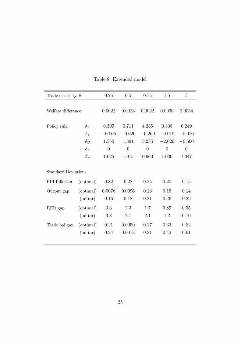
Table 8: Extended model

Trade elasticity, 025 05 075 15 3

Welfare difference 00022 00023 00022 00030 00034

Policy rule 0395 0711 4285 0338 0249

−0005 −0020 −0269 −0010 −0010D 1550 1891 3235 −2026 −0600L 0 0 0 0 0

1025 1015 0960 1030 1047

Standard Deviations

PPI Inflation (optimal) 032 028 025 020 015

Output gap (optimal) 00076 00096 013 015 014

(inf tar) 016 018 021 026 029

RER gap (optimal) 33 23 17 089 055

(inf tar) 38 27 21 12 070

Trade bal gap (optimal) 021 00050 017 033 052

(inf tar) 024 00073 021 042 061

25

recent literature, optimal monetary policy deviates from inflation targeting in order to

offset exchange rate misalignments, but the welfare difference between optimal policy and

inflation targeting is quantitatively smaller than found in the simpler models of financial

incompleteness analysed in Corsetti et al (2010, 2011). It is found, however, that optimal

policy does imply quantitatively significant stabilisation of the real exchange rate gap

and the trade balance gap compared to inflation targeting.

This paper focuses on a model of imperfect financial markets where the imperfection

simply takes the form of a restricted set of financial instruments (i.e. bonds and equities)

which is insufficient to provide full international risk sharing. Devereux and Sutherland

(2011b) show that the presence of collateral constraints can significantly alter the inter-

national transmission of shocks, especially in the case when there is trade in bonds and

equity. In a companion paper (Senay and Sutherland, 2016) we analyse optimal monetary

policy in a version of the above model which has been extended to incorporate the form

of collateral constraints introduced in Devereux and Sutherland (2011b).

26

References

Beaudry, P. and F. Portier (2006) “Stock Prices, News, and Economic Fluctuations”

American Economic Review, 96, 1293-1307.

Benigno, P. (2009) “Price Stability with Imperfect Financial Integration” Journal of

Money, Credit and Banking, 41, 121-149.

Benigno, P. and M. Woodford (2005) “Inflation Stabilization and Welfare: The Case of a

Distorted Steady State” Journal of the European Economic Association, 3, 1185-1236.

Benigno, G. and Benigno, P. (2003) “Price Stability in Open Economies” Review of

Economics Studies 70, 743-764.

Calvo, G. A. (1983) “Staggered Prices in a Utility-Maximizing Framework” Journal of

Monetary Economics, 12, 383-398.

Christiano, L., M. Eichenbaum and C Evans (2005) “Nominal rigidities and the dynamic

effects of a shock to monetary policy” Journal of Political Economy, 113, 1-45.

Clarida, R., Gali J. and Gertler, M. (2002) “A Simple Framework for International Mon-

etary Policy Analysis” Journal of Monetary Economics, 49, 879-904.

Corsetti, G., L. Dedola and S Leduc (2010) "Optimal Monetary Policy in Open

Economies" in Handbook of Monetary Economics Vol.3B Ben Friedman and Michael

Woodford (eds)., Elsevier, 862-933.

Corsetti, G., L. Dedola and S Leduc (2011) "Demand Imbalances, Exchange Rate Mis-

alignment and Monetary Policy" mimeo.

Damjanovic, T., Damjanovic, V., and Nolan, C. (2008) “Unconditionally optimal mone-

tary policy” Journal of Monetary Economics, 55, 491-500.

Devereux, M. and A. Sutherland (2008) “Financial globalization and monetary policy”

Journal of Monetary Economics, 55, 1363-1375.

Devereux, M. and A. Sutherland (2010) “Country portfolio dynamics” Journal of Eco-

nomic Dynamics and Control, 34, 1325-1342.

Devereux, M. and A. Sutherland (2011a) “Solving for country portfolios in open economy

macro models” Journal of the European Economic Association, 9, 337-369.

27

Devereux, M. and A. Sutherland (2011b) “Evaluating International Financial Integration

Under Leverage Constraints” European Economic Review, 55, 427-442.

Devereux, M., O. Senay, and A. Sutherland (2014) “Nominal Stability and Financial

Globalization” Journal of Money, Credit and Banking 46, 5, 921-939.

De Paoli, B. (2010) “Monetary Policy under Alternative Asset Market Structures: The

Case of a Small Open Economy” Journal of Money, Credit, and Banking, 41, 1301-1330.

Engel, C. (2011) “Currency misalignments and optimal monetary policy: a re-

examination” American Economic Review, 101, 2796-2822.

Gali, J. and Monacelli, T. (2005) “Monetary Policy and Exchange Rate Volatility in a

Small Open Economy” Review of Economics Studies, 72, 707-734.

Schmitt-Grohe, S. and M. Uribe (2003) “Closing Small Open Economy Models” Journal

of International Economics, 59, 137-59.

Senay, O. and A. Sutherland (2016) “Country Portfolios, Collateral Constraints and

Optimal Monetary Policy” unpublished manuscript, University of St Andrews.

Smets F. and R. Wouters (2003) “An estimated dynamic stochastic general equilibrium

model of the euro area” Journal of the European Economic Association, 5, 1123-1175.

Smets F. and R. Wouters (2005) “Comparing shocks and frictions in US and euro area

business cycles: a Bayesian DSGE approach” Journal of Applied Econometrics, 20,

161-183.

Smets F. and R. Wouters (2007) “Shocks and frictions in US business cycles: a Bayesian

DSGE approach” American Economic Review, 97.

Tille, C. and E. vanWincoop (2010) “International capital flows” Journal of International

Economics, 80, 157-175.

Woodford, M. (2003) Interest and Prices: Foundations of a Theory of Monetary Policy

Princeton University Press, Princeton, NJ.

28