optics notes master - RIT Center for Imaging Science · Course Notes for IMGS-321 11 December 2013...
204
Ray Optics for Imaging Systems Course Notes for IMGS-321 11 December 2013 Roger Easton Chester F. Carlson Center for Imaging Science Rochester Institute of Technology 54 Lomb Memorial Drive Rochester, NY 14623 1-585-475-5969 [email protected] December 11, 2013
-
Upload
truongkhuong -
Category
Documents
-
view
222 -
download
2
Transcript of optics notes master - RIT Center for Imaging Science · Course Notes for IMGS-321 11 December 2013...

Ray Optics for Imaging SystemsCourse Notes for IMGS-321
11 December 2013
Roger Easton
Chester F. Carlson Center for Imaging Science
Rochester Institute of Technology
54 Lomb Memorial Drive
Rochester, NY 14623
1-585-475-5969
December 11, 2013

Contents
Preface ix0.1 References: . . . . . . . . . . . . . . . . . . . . . . . . . . . . . . . . . . . . . . . . . 1
1 Introduction 11.1 Models of Light and Propagation . . . . . . . . . . . . . . . . . . . . . . . . . . . . . 2
1.1.1 Ray model of light (“geometrical optics”) . . . . . . . . . . . . . . . . . . . . 21.1.2 Wave model of light (“physical optics”): . . . . . . . . . . . . . . . . . . . . . 21.1.3 Photon model of light (“quantum optics”): . . . . . . . . . . . . . . . . . . . 3
2 Ray (Geometric) Optics 52.1 What is an imaging system? . . . . . . . . . . . . . . . . . . . . . . . . . . . . . . . . 5
2.1.1 Simplest Imaging System — Pinhole in Absorber . . . . . . . . . . . . . . . . 52.2 First-Order Optics . . . . . . . . . . . . . . . . . . . . . . . . . . . . . . . . . . . . . 62.3 Third-Order Optics . . . . . . . . . . . . . . . . . . . . . . . . . . . . . . . . . . . . . 9
2.3.1 Higher-Order Approximations . . . . . . . . . . . . . . . . . . . . . . . . . . . 102.4 Notations and Sign Conventions . . . . . . . . . . . . . . . . . . . . . . . . . . . . . 10
2.4.1 Nature of Objects and Images: . . . . . . . . . . . . . . . . . . . . . . . . . . 112.5 Human Eye . . . . . . . . . . . . . . . . . . . . . . . . . . . . . . . . . . . . . . . . . 132.6 Principle of Least Time . . . . . . . . . . . . . . . . . . . . . . . . . . . . . . . . . . 132.7 Fermat’s Principle for Reflection . . . . . . . . . . . . . . . . . . . . . . . . . . . . . 14
2.7.1 Plane Mirrors . . . . . . . . . . . . . . . . . . . . . . . . . . . . . . . . . . . . 172.8 Fermat’s Principle for Refraction: . . . . . . . . . . . . . . . . . . . . . . . . . . . . . 18
2.8.1 Dispersion . . . . . . . . . . . . . . . . . . . . . . . . . . . . . . . . . . . . . . 192.8.2 Refractive Constants for Glasses . . . . . . . . . . . . . . . . . . . . . . . . . 21
2.9 Image Formation in the Ray Model . . . . . . . . . . . . . . . . . . . . . . . . . . . . 242.9.1 Refraction at a Spherical Surface . . . . . . . . . . . . . . . . . . . . . . . . . 242.9.2 Imaging with Spherical Mirrors . . . . . . . . . . . . . . . . . . . . . . . . . . 27
2.10 First-Order Imaging with Thin Lenses . . . . . . . . . . . . . . . . . . . . . . . . . . 282.10.1 Examples of Thin Lenses . . . . . . . . . . . . . . . . . . . . . . . . . . . . . 302.10.2 Spherical Mirror . . . . . . . . . . . . . . . . . . . . . . . . . . . . . . . . . . 32
2.11 Image Magnifications . . . . . . . . . . . . . . . . . . . . . . . . . . . . . . . . . . . . 322.11.1 Transverse Magnification: . . . . . . . . . . . . . . . . . . . . . . . . . . . . . 322.11.2 Longitudinal Magnification: . . . . . . . . . . . . . . . . . . . . . . . . . . . . 332.11.3 Angular Magnification . . . . . . . . . . . . . . . . . . . . . . . . . . . . . . . 34
2.12 Single Thin Lenses . . . . . . . . . . . . . . . . . . . . . . . . . . . . . . . . . . . . . 352.12.1 Positive Lens . . . . . . . . . . . . . . . . . . . . . . . . . . . . . . . . . . . . 352.12.2 Negative Lens . . . . . . . . . . . . . . . . . . . . . . . . . . . . . . . . . . . . 362.12.3 Meniscus Lenses . . . . . . . . . . . . . . . . . . . . . . . . . . . . . . . . . . 362.12.4 Simple Microscope (magnifier, “magnifying glass,” “loupe”) . . . . . . . . . . 37
2.13 Systems of Thin Lenses . . . . . . . . . . . . . . . . . . . . . . . . . . . . . . . . . . 412.13.1 Two-Lens System . . . . . . . . . . . . . . . . . . . . . . . . . . . . . . . . . . 412.13.2 Effective (Equivalent) Focal Length . . . . . . . . . . . . . . . . . . . . . . . 43
v

vi CONTENTS
2.13.3 Summary of Distances for Two-Lens System . . . . . . . . . . . . . . . . . . . 482.13.4 “Effective Power” of Two-Lens System . . . . . . . . . . . . . . . . . . . . . . 482.13.5 Lenses in Contact: t = 0 . . . . . . . . . . . . . . . . . . . . . . . . . . . . . . 492.13.6 Positive Lenses Separated by t < f1 + f2 . . . . . . . . . . . . . . . . . . . . . 492.13.7 Cardinal Points . . . . . . . . . . . . . . . . . . . . . . . . . . . . . . . . . . . 552.13.8 Lenses separated by t = f1 + f2: Afocal System (Telescope) . . . . . . . . . . 562.13.9 Positive Lenses Separated by t = f1 or t = f2 . . . . . . . . . . . . . . . . . . 582.13.10Positive Lenses Separated by t > f1 + f2 . . . . . . . . . . . . . . . . . . . . . 602.13.11Compound Microscopes . . . . . . . . . . . . . . . . . . . . . . . . . . . . . . 612.13.12Two Positive Lenses with Different Focal Lengths and Different Separations . 622.13.13Systems of One Positive and One Negative Lens . . . . . . . . . . . . . . . . 632.13.14Newtonian Form of Imaging Equation . . . . . . . . . . . . . . . . . . . . . . 642.13.15Example (1) of Two-Lens System . . . . . . . . . . . . . . . . . . . . . . . . . 652.13.16Example (2) of Two-Lens System: Telephoto Lens . . . . . . . . . . . . . . . 692.13.17 Images from Telephoto System: . . . . . . . . . . . . . . . . . . . . . . . . . . 722.13.18Example (3) of Two-Lens System: Two Negative Lenses . . . . . . . . . . . . 74
2.14 Plane and Spherical Mirrors . . . . . . . . . . . . . . . . . . . . . . . . . . . . . . . . 762.14.1 Comparison of Thin Lens and Concave Mirror . . . . . . . . . . . . . . . . . 79
2.15 Stops and Pupils . . . . . . . . . . . . . . . . . . . . . . . . . . . . . . . . . . . . . . 792.15.1 Focal Ratio — f-number . . . . . . . . . . . . . . . . . . . . . . . . . . . . . . 802.15.2 Example: Focal Ratio of Lens-Aperture Systems . . . . . . . . . . . . . . . . 812.15.3 Example: Exit Pupils of Telescopic Systems . . . . . . . . . . . . . . . . . . . 852.15.4 Pupils and Diffraction . . . . . . . . . . . . . . . . . . . . . . . . . . . . . . . 902.15.5 Field Stop . . . . . . . . . . . . . . . . . . . . . . . . . . . . . . . . . . . . . . 91
2.16 Marginal and Chief Rays . . . . . . . . . . . . . . . . . . . . . . . . . . . . . . . . . . 912.16.1 Telecentricity . . . . . . . . . . . . . . . . . . . . . . . . . . . . . . . . . . . . 922.16.2 Marginal and Chief Rays for Telescopes . . . . . . . . . . . . . . . . . . . . . 94
3 Tracing Rays Through Optical Systems 953.1 Paraxial Ray Tracing Equations . . . . . . . . . . . . . . . . . . . . . . . . . . . . . . 95
3.1.1 Paraxial Refraction . . . . . . . . . . . . . . . . . . . . . . . . . . . . . . . . . 963.1.2 Paraxial Transfer . . . . . . . . . . . . . . . . . . . . . . . . . . . . . . . . . . 973.1.3 Linearity of the Paraxial Refraction and Transfer Equations . . . . . . . . . . 983.1.4 Paraxial Ray Tracing . . . . . . . . . . . . . . . . . . . . . . . . . . . . . . . 98
3.2 Matrix Formulation of Paraxial Ray Tracing . . . . . . . . . . . . . . . . . . . . . . . 1003.2.1 Refraction Matrix . . . . . . . . . . . . . . . . . . . . . . . . . . . . . . . . . 1013.2.2 Ray Transfer Matrix . . . . . . . . . . . . . . . . . . . . . . . . . . . . . . . . 1023.2.3 “Vertex-to-Vertex Matrix” for System . . . . . . . . . . . . . . . . . . . . . . 1043.2.4 Example 1: System of Two Positive Thin Lenses . . . . . . . . . . . . . . . . 1053.2.5 Example 2: Telephoto Lens . . . . . . . . . . . . . . . . . . . . . . . . . . . . 1083.2.6 MVV0 Derived From Two Rays . . . . . . . . . . . . . . . . . . . . . . . . . . 109
3.3 Object-to-Image (Conjugate) Matrix . . . . . . . . . . . . . . . . . . . . . . . . . . . 1103.3.1 Matrix of the “Relaxed” Eye (focused at ∞) . . . . . . . . . . . . . . . . . . 114
3.4 Vertex-Vertex Matrices of Simple Imaging Systems . . . . . . . . . . . . . . . . . . . 1153.4.1 Magnifier (“magnifying glass,” “loupe”) . . . . . . . . . . . . . . . . . . . . . 1153.4.2 Galilean Telescope of Thin Lenses . . . . . . . . . . . . . . . . . . . . . . . . 1163.4.3 Keplerian Telescope of Thin Lenses . . . . . . . . . . . . . . . . . . . . . . . . 1173.4.4 Thick Lenses . . . . . . . . . . . . . . . . . . . . . . . . . . . . . . . . . . . . 1173.4.5 Microscope . . . . . . . . . . . . . . . . . . . . . . . . . . . . . . . . . . . . . 121
3.5 Image Location and Magnification . . . . . . . . . . . . . . . . . . . . . . . . . . . . 1223.6 Marginal and Chief Rays for the System . . . . . . . . . . . . . . . . . . . . . . . . . 122
3.6.1 Examples of Marginal and Chief Rays for Systems . . . . . . . . . . . . . . . 123

CONTENTS vii
4 Depth of Field and Depth of Focus 1414.0.2 Examples of Depth of Field from Video and Film . . . . . . . . . . . . . . . . 143
4.1 Criterion for “Acceptable Blur” . . . . . . . . . . . . . . . . . . . . . . . . . . . . . . 1494.2 Depth of Field via Rayleigh’s Quarter-Wave Rule . . . . . . . . . . . . . . . . . . . . 1524.3 Hyperfocal Distance . . . . . . . . . . . . . . . . . . . . . . . . . . . . . . . . . . . . 1564.4 Methods for Increasing Depth of Field . . . . . . . . . . . . . . . . . . . . . . . . . . 1564.5 Sidebar: Transverse Magnification vs. Focal Length . . . . . . . . . . . . . . . . . . 157
5 Aberrations 1615.1 Chromatic Aberration . . . . . . . . . . . . . . . . . . . . . . . . . . . . . . . . . . . 1615.2 Third-Order Optics, Monochromatic Aberrations . . . . . . . . . . . . . . . . . . . . 165
5.2.1 Names of Aberrations . . . . . . . . . . . . . . . . . . . . . . . . . . . . . . . 1735.2.2 Aberration Coefficients . . . . . . . . . . . . . . . . . . . . . . . . . . . . . . 1745.2.3 Fourth-Order (Third-Order Ray) Aberrations: . . . . . . . . . . . . . . . . . . 1815.2.4 Zernike Polynomials . . . . . . . . . . . . . . . . . . . . . . . . . . . . . . . . 190
5.3 Structural Aberration Coefficients . . . . . . . . . . . . . . . . . . . . . . . . . . . . 1935.4 Optical Imaging Systems and Sampling . . . . . . . . . . . . . . . . . . . . . . . . . 1935.5 Optical System “Rules of Thumb” . . . . . . . . . . . . . . . . . . . . . . . . . . . . 193

Preface
This book is intended to introduce the mathematical tools that can be applied to model and predictthe action of optical imaging systems.
ix


0.1 REFERENCES: 1
0.1 References:Many references exist for the subject of wave optics, some from the point of view of physics and manyothers from the subdiscipline of optics. Unfortunately, relatively few from either camp concentrateon the aspects that are most relevant to imaging.
Useful Optics Texts:
[P3] (the three) Pedrottis, Introduction to Optics, Pearson Prentice-Hall, 2007.[G] Gaskill, Jack D., Linear Systems, Fourier Transforms, and Optics, John Wiley, 1978.[JG] Goodman, Joseph, Introduction to Fourier Optics, Third Edition, Roberts & Company,
2005.[H] Eugene Hecht, Optics, 4th Edition, Addison-Wesley, 2002.[PON] Reynolds, DeVelis, Parrent, Thompson, The New Physical Optics Notebook, SPIE,
1989.[BW] Max Born and Emil Wolf, Principles of Optics, 7th Expanded Edition, Cambridge
University Press, 2005.[GF] Grant R. Fowles, Introduction to Modern Optics (Second Edition), Dover Publications,
1975.[RHW] Robert H. Webb, Elementary Wave Optics, Dover Publications, 1997.[FLS] R. Feynman, R. Leighton, M. Sands, The Feynman Lectures on Physics, Addison-
Wesley, 1964.[KF] M.V. Klein and T.E. Furtak, Optics, Second Edition, Wiley, 1986[JW] F. Jenkins and H. White, Fundamentals of Optics, 4th Edition, McGraw-Hill, 1976.[NP] A. Nussbaum and R. Phillips, Contemporary Optics for Scientists and Engineers,
Prentice-Hall, 1976.[I] K. Iizuka, Engineering Optics, Springer-Verlag, 1985.[FBS] D. Falk, D. Brill, and D. Stork, Seeing the Light, Harper and Row, 1986.Lawrence Mertz, Transformations in Optics, John Wiley & Sons, 1965.
Physics Texts with useful discussions:
[HR] D. Halliday and R. Resnick, Physics, 3rd Edition, Wiley, 1978.[C] F. Crawford,Waves, Berkeley Physics Series Vol. III, McGraw-Hill, 1968.John D. Jackson, Classical Electrodynamics, Third Edition, Wiley, 1998, §6.Feynman, Leighton, and Sands, Lectures on Physics, particularly Volume 1.§25-§33 and Vol-
ume II §32-§33
Curriculum: Geometrical Optics and Imaging1. Models for light propagation
(a) ray model (“geometric optics”)
(b) wave model (“physical optics”)
(c) photon model (quantum optics)
2. First-order optics
(a) third-order optics, aberrations
(b) higher-order approximations
3. Sign conventions for distances and angles
(a) Nature of objects and images (real and virtual)

2 Preface
4. Human eye
5. Refractive index
(a) Optical path length
(b) Fermat’s principle of least time (P3 §2.2, H §4.5, BW §3.3)
(c) Snell’s law for reflection: θ2 = −θ1i. plane mirrors
(d) Snell’s law for refraction: n1 sin [θ1] = n2 sin [θ2]
i. plane interface between two media
(e) Dispersion (variation in n with λ)
i. relationship between mean refractive index and dispersionii. crown and flint glasses
(f) Dispersing prisms
6. Refraction at a Spherical Surface
(a) Paraxial approximation, imaging equation
(b) Reflection at a spherical surface
7. Imaging with thin lenses
(a) Imaging equation in terms of object and image distances and focal length
(b) system “power”
(c) spherical mirrors
(d) object/image conjugates
(e) Image magnifications
i. Transverse magnificationii. Longitudinal magnificationiii. Angular magnification
(f) Single thin lenses
i. positive lensii. negative lensiii. meniscus lensiv. simple microscope
(g) Systems of thin lenses
i. lenses in contactii. effective focal length and power of two-lens systemiii. focal and principal pointsiv. afocal systems (telescopes)v. eyeglassesvi. compound microscopesvii. Newtonian form of imaging equationviii. telephoto lensix. Stops and pupils
A. aperture stopB. entrance and exit pupils

0.1 REFERENCES: 3
C. field stop
(h) Marginal and chief (principal) rays
i. telecentricity
8. Tracing rays through optical systems
(a) paraxial ray tracing equations
i. paraxial refractiontransferii. paraxial transferiii. linearity of equations
(b) matrix formulation of paraxial ray tracing
i. refraction matrixii. transfer matrixiii. Lagrangian invariantiv. vertex-to-vertex matrix for imaging systemv. object-to-image (conjugate) matrixvi. matrix for eye model
(c) Examples of imaging system matrices
i. magnifierii. Galilean telescopeiii. Keplerian telescopeiv. thick lensv. microscope
(d) image location and magnification
(e) Depth of field and depth of focus
i. examples from film and videoii. criterion for “acceptable blur”iii. depth of field via Rayleigh’s quarter-wave ruleiv. hyperfocal distancev. methods for increasing depth of fieldvi. transverse magnification vs. focal length
(f) Aberrations
i. Chromatic aberrationA. achromatic doubletB. apochromatic triplet
ii. Third-Order (Seidel) AberrationsA. spherical aberration (relation to defocus)B. comaC. astigmatismD. distortionE. curvature of fieldF. piston error
9. Computed Ray Tracing, OSLOTM


Chapter 1
Introduction
The obvious first question to consider is “what is optics” (or perhaps “what are optics?” heh, heh).One reasonable definition of optics is the application of physical principles and observed phenomenato manipulate “light” in useful ways. This presupposes the definition of “light,” which I specify aselectromagnetic radiation of any “color,” temporal frequency, and wavelength. This is more generalthan the definition put forth by humanocentrics (e.g., color scientists), but is much more reasonablein our field, where we want to take advantage of all measureable radiation to learn informationabout objects that emit, reflect, refract, or otherwise modify radiation. The definition in imagingis somewhat narrower: the application of the properties if materials and of light to form “images,”which are “recognizable (though approximate) replicas of the spatial and spectral distribution oflight reflected, transmitted, and/or emitted by an object.”To design optical image-forming systems, we must model the propagation of light from the
object (source) to the optic, the action of the optic on the incident light distribution, and finallypropagation from the optic to the sensor. The last step of conversion of the spatial (and possiblyspectral) distribution of incident light into measurable physical and/or chemical changes in somemedium by the sensor, is outside the scope of this discussion.We hope to find a mathematical model of optical imaging as a “system,” where an output dis-
tribution g is created from an input object distribution f by the action of an imaging system O,e.g., g [x, y, λ] = O{f [x, y, z, λ]}. We generally use this model to (try to) solve the inverse imagingproblem by inferring the input object from the output image and knowledge of the system. The taskmay be difficult or even impossible; it is easy to see one difficulty because most sensors measure onlya 2-D distribution of monochromatic light and therefore cannot possibly recover the three spatialdimensions of a realistic object from a single image.
Schematic of an optical system that acts on an input with three spatial dimensions, time, andwavelength f [x, y, z, t, λ] to produce a 2-D monochrome (gray scale) image g [x0, y0].
1

2 CHAPTER 1 INTRODUCTION
1.1 Models of Light and PropagationTo be able even to write down, let alone solve, the imaging equation(s) for optical systems, weneed to specify the mathematical model of light that will describe its behavior as it propagates andinteracts with input objects, optical systems, and output sensors. To simplify the descriptions inthe different contexts, three physical models for light and its interactions are used that are (looselyspeaking) distinguished by the physical scale of the phenomena:
1.1.1 Ray model of light (“geometrical optics”)
macroscopic-scale phenomena (e.g., reflection, refraction)
1. (a) light propagates as RAYS that travel in straight lines until encountering an change inproperties of a medium or an interface between media. Except to differentiate the colorof light, the wavelength λ and temporal frequency ν of the light are assumed to be zeroand infinity, respectively (λ→0, ν→∞), which means that there are no effects due todiffraction;
(b) uses Fermat’s principle of least time to derive Snell’s law, which describes the phenomenaof reflection and refraction;
(c) useful for designing imaging systems (to locate the images and determine their magnifi-cations)
(d) calculations for modeling the behavior of optical systems (lenses and/or mirrors) are(relatively) simple and may be easily implemented in software;
(e) the quality of images from the system is assessed in terms of aberrations of the opticalsystem, which describe deviations of the image from ideal behavior.
1.1.2 Wave model of light (“physical optics”):
1. microscopic-scale phenomena (diffraction/interference, reflection, refraction, refractive index,...)
(a) considers light (electromagnetic radiation) to propagate as WAVES ;
(b) propagation and interaction of light are described by Maxwell’s equations ;
(c) light propagates with velocity c in vacuum¡c / 3× 10⁸ms−1
¢and velocity v < c in
transparent materials;
(d) light is described by its wavelength in vacuum λ0 and oscillation frequency ν0, whosevalues affect any interactions with matter;
(e) the oscillation frequency ν0 of waves emitted by a particular light source is constantregardless of medium and is related to the vacuum wavelength λ0 via:
λ0 · ν0 = c
(f) the ratio of the propagation velocities in vacuum and in a medium is the index of refractionof the medium:
n ≡ c
v
(g) the wavelength of the wave in a medium is shorter the “vacuum wavelength” λ0 via:
λmedium =λ0n
(h) wave optics explains the image-forming phenomena of reflection, refraction, diffraction(and interference, which is really just another name for diffraction) and the phenomenaof polarization and dispersion that affect the quality of images;

1.1 MODELS OF LIGHT AND PROPAGATION 3
(i) mathematical calculations in wave optics are more “complicated” than those in ray opticsand often not easy to implement in computers. For example, it is difficult to evaluate theexact form of light after propagating a short distance from the source;
(j) uses the Huygens-Fresnel principle to derive the mathematical model for propagation oflight, which if often divided into three regions:
i. linear, shift-invariant model in the Rayleigh-Sommerfeld diffraction region (valideverywhere)
ii. linear, shift-invariant approximation in the near field for propagation by a “suffi-ciently large” distance from the source (Fresnel diffraction)
iii. linear, shift-variant approximation in the far field for propagation to “very large”distances from the source (Fraunhofer diffraction);
(k) wave/physical optics is useful for assessing the quality of the images produced by systems.
1.1.3 Photon model of light (“quantum optics”):
atomic-scale phenomena (emission and absorption of radiation)
1. (a) light is composed of PHOTONS with both wave and particle characteristics;
(b) used to explain/analyze the physical interaction of light and matter, such as emission bysources (e.g., lasers), and the photoelectric effect in sensors;
(c) Fundamental relationships: E0 = hν0 = hc
λ0and momentum p =
E
c=
h
λ0, where h is
Planck’s constant:h ∼= 6.626× 10⁻³⁴ J s ∼= 4.136× 10⁻¹⁵ eV s
Phenomena described by the ray and wave models are most relevant to imaging, though thequantum model is vital for understanding the properties and artifacts of light sensing. You probablyhave seen some consideration of ray optics in undergraduate physics, and any such experience willbe useful in this course. The most common treatments of optics consider rays first because themathematical models and calculations are simpler. However, the preparation of linear systems youjust had makes it possible and even desirable to consider the wave model first by applying theconcepts of the impulse response and transfer function; these may significantly simplify the conceptsand calculations.There are several goals to be reached by the conclusion of this discussion; we want to have the
capabilities to do several things:
• locate the image(s) of an object generated by the lens, mirror, or system of lenses and/ormirrors;
• determine the “character” (real or virtual) and the size(s) (i.e., the transverse magnification)of the image(s);
• determine the “field of view” of the imaging system, i.e., the angular subtense of the objectthat is imaged;
• determine the range of distances in the scene from the optical system that appears to be “infocus” (the depth of field);
• determine the capability of the optics to distinguish closely spaced objects — this is the “spatialresolution” of the system (often specified in terms of measurements from the “point spreadfunction” or the “modulation transfer function” = “MTF,” which are optical analogues ofthe “impulse response” and “transfer function” that are considered in the course on Fouriermethods);

4 CHAPTER 1 INTRODUCTION
• understand the constraints on system performance due to the properties of materials used in theimaging system, such as the variation in refractive index of glass with wavelength (dispersion)
Much of this discussion (especially about depth of field and spatial resolution) will benefit fromconcepts derived in the course on Fourier methods, but we must also be aware of the limitations inthese concepts due to nonlinearities and/or shift-variant properties of the optical system.

Chapter 2
Ray (Geometric) Optics
Ray optics (commonly, though unfortunately, called “geometric optics”) uses the model of light as aray to evaluate the locations and properties of images created by systems of lenses and/or mirrors.It does not consider any effects due to the wave model of light, such as interference or diffraction(which are actually just different words for the same phenomenon: “interference” considers few lightsources and “diffraction” considers an infinite number, or just “many”). The subject of ray opticsmay be subdivided into categories of “first-order,” “third-order,” and even higher-order opticalcomputations. It also cannot explain other wave-propagation phenomena, such as total internalreflection.
2.1 What is an imaging system?As a simple definition, we may consider an imaging system to map the distribution of the input“object” to a “similar” distribution at the output “image” (where the meaning of “similar” is to bedetermined). Often the input and output amplitudes are represented in different units. For example,the input often is electromagnetic radiation with units of, say, watts per unit area, while the outputmay be a transparent negative emulsion measured in dimensionless units of “density” or “transmit-tance.” In other words, the system often changes the form of the energy; it is a “transducer.”In the ray model, we can think of the imaging system as “selecting” and/or “redirecting” rays of
light to map the energy onto the image sensor. The “selection” or “redirection” process uses sometype of physical interaction between light and matter to remap the energy emitted or modified bythe object onto the sensor. Among the more obvious physical interactions in our experience arerefraction and reflection, but these are not the only, nor even the simplest, possible mechanisms.The very simplest interaction between light and matter is absorption, where the light energy istransferred to matter and “disappears” (of course, it does not really “vanish,” but most often isconverted into heat in the matter, but it is no longer available to create an image, so it may as wellhave “disappeared.” We can use an absorber to create the simplest imaging system: the pinholecamera
2.1.1 Simplest Imaging System — Pinhole in Absorber
Consider a 3-D volume of space that contains the object. Occasionally, a ray of light emitted (orreflected) from a location in the volume is selected by the pinhole and reaches the sensor.
every point in space is “in focus” on the sensortransverse magnification Mt determined by relative distances
MT = −z2z1
negative sign means image is inverted
5

6 CHAPTER 2 RAY (GEOMETRIC) OPTICS
The number of rays from the object that actually reach the image is small. The interactionwith the sensor requires the quantum model of discrete energy packets, so the number of packetsis small if the hole diameter is small. If the object is a uniformly emitting planar source, thenumbers of packets measured from different locations in the field are different (Poisson statistics);these numerical variations in what should be identical measurements appear as “noise.” The metricof noise is determined by the mean value μ of the signal and the variation about that mean, whichis described by the standard deviation σ. The signal-to-noise ratio is a dimensionless quantity thatmay be defined many ways, but we’ll use a simple definition that will suit this purpose
SNR ≡ μ
σ=
μ√μ=√μ
More photons leads to larger signals (μ ↑) and larger standard deviation (σ ↑), but mean increasesfaster than the variance σ =
√μ, so the SNR is
better statistics and less relative noise“Quality” of image depends on diameter d0 of pinhole. Improve statistics by increasing the
number of photons. Larger dose or larger pinhole. The “blur” quality of the image is better forsmaller pinhole because less uncertainty in ray path.How to improve?Longer exposure timemultiple pinholes
Depth of field
Redirect rays:reflective pinholesReflectionRefractionDiffraction (wave property), e.g., holography
2.2 First-Order Optics
Of most concern to us will be “first-order,” “paraxial ” or “Gaussian” optics, where the angles oflight rays measured relative to the optical axis are assumed to be small, so that the ray heightsremain small as the rays propagate down the optical axis, which is the source of another commonterm of “paraxial optics,” meaning that the ray remains near the optical axis. In cases such thatthe ray angle θ ∼= 0, then we can approximate trigonometric functions by the first terms in theirpower-series expansions (the “Taylor series” ):
f [x] =(x− x0)
0
0!· f [x0] +
(x− x0)1
1!
Ãdf
dx
¯x=x0
!+(x− x0)
2
2!
Ãd2f
dx2
¯x=x0
!+ · · ·+ 1
n!· d
nf
dxn
¯x=x0
· (x− x0)n + · · ·
=∞Xn=0
(x− x0)n
n!· f (n) [x0]
If the base value and the derivatives are evaluated at the origin, we have a “Maclaurin series:”
f [x] =∞Xn=0
1
n!f (n) [0] · xn

2.2 FIRST-ORDER OPTICS 7
The Maclaurin series for the sine is:
sin [θ] =∞Xn=0
1
n!· dn
dθn(sin [θ])
¯θ=0
· θn
sin [θ] =1
0!· sin [0] · θ0 + 1
1!· (+ cos [0]) · θ1 + 1
2!· (− sin [0]) · θ2 + 1
3!· (− cos [0]) · θ3 + 1
4!· (+ sin [0]) · θ4 + · · ·
= 0 + θ + 0− θ3
3!+ 0 +
θ5
5!− · · ·
= θ − θ3
3!+
θ5
5!− · · ·
= θ − θ3
6+
θ5
120− · · ·
Note that only odd powers of θ are present in the series for sin [θ], because the sine is an odd(antisymmetric) function that satisfies the condition sin [−θ] = − sin [+θ].
The corresponding series for the even (or symmetric) cosine includes only even powers of θ:
cos [θ] = 1− θ2
2!+
θ4
4!− · · · =
∞Xn=0
(−1)n θ2n
(2n)!
=⇒ limθ∼=0
{cos [θ]} = 1
=⇒ cos [θ] ≡ 1− θ2
2
So the approximation of the cosine with two terms is the difference of a constant and a parabola.
The series for the (odd, antisymmetric) tangent is less commonly known and includes only theodd powers of θ:
tan [θ] = θ +θ3
3+2
15θ5 + · · · =
∞Xn=0
¡22n¢ ¡22n − 1¢
(2n)!B2n θ2n−1 =⇒ lim
θ∼=0{tan [θ]} = θ
where B isbthe th Bernoulli number. The first-, third-, and fifth-order series approximations forthe tangent are:
tan [θ] ∼= θ forπ
2> |θ| ' 0
tan [θ] ∼= θ +θ3
3
tan [θ] ∼= θ +θ3
3+2
15θ5
The validity of these approximations is perhaps more obvious from the graphs, where we can seethat sin [θ] / θ and tan [θ] ' θ for small positive values of θ.

8 CHAPTER 2 RAY (GEOMETRIC) OPTICS
0.0 0.1 0.2 0.3 0.4 0.50.0
0.1
0.2
0.3
0.4
0.5
theta
Comparison of θ (black), sin [θ] (red), and tan [θ] (blue) for 0 ≤ θ ≤ +0.5 radians, showing thatsin [θ] / θ and tan [θ] ' θ over this domain.
The corresponding first-order approximation to the cosine is the unit constant
limθ→0
{cos [θ]} = 1
0.00 0.02 0.04 0.06 0.08 0.10 0.12 0.14 0.16 0.18 0.200.8
0.9
1.0
1.1
1.2
theta
The first-order approximation to cos [θ] (red) compared to the unit constant (black), showing thatthe two are very similar for small values of θ.
The advantage of the first-order approxmation is that evaluation of the ray heights and anglesbecomes simple because of the proportionality.

2.3 THIRD-ORDER OPTICS 9
2.3 Third-Order OpticsIt likely is obvious from the definition of first-order optics that “third-order” optics includes thesecond term in the expansions:
sin [θ] ∼= θ − θ3
3!= θ − θ3
6
tan [θ] ∼= θ +θ3
3
cos [θ] ∼= 1− θ2
2!= 1− θ2
2
0.0 0.1 0.2 0.3 0.4 0.50.0
0.1
0.2
0.3
0.4
0.5
theta
Comparison third-order approximations of sin [θ] (red), and tan [θ] (blue) to the linear term θ(black) .
Note that the third-order approximation for the cosine is a biased parabola:
0.0 0.1 0.2 0.3 0.4 0.50.8
0.9
1.0
1.1
1.2
theta
cos [θ] (black) and its third-order approximation as 1− θ2
2 (red).

10 CHAPTER 2 RAY (GEOMETRIC) OPTICS
The results for ray angles using third-order optics will differ from those of first-order optics; thesedifferences lead to image aberrations.
2.3.1 Higher-Order Approximations
We clearly can add additional terms to the power series that will increase the accuracy of anycalculations at the cost of significantly more complexity.
2.4 Notations and Sign Conventions
One of the simplest and most difficult aspects of ray optics is the set of conventions to be adopted forall of the quantities to be measured. As in many aspects of optics, there are competing choices forconventions that have their own distinct advantages, but that lead to different equations for imagelocations, etc. We are going to use the directed distance convention, where distances are positiveif measured from left to right. The problem becomes remembering which are the points measured“from” and “to,” respectively. The figure shows sign conventions for the different quantities. Notethat in all cases, light travels from left to right in all media with positive refractive index (n > 0), sothe distances are positive if measured in the same direction of light travel and negative if measuredin the other direction.
Sign conventions for distances, heights, angles, and curvatures. The distance is positive if measuredfrom left to right; the height is positive if the endpoint is above the axis; the angle from the axis orfrom a normal is positive if measured in the counterclockwise direction (positive θ); and the
curvature is positive if its center is to the right of the vertex (intersection of the surface and theoptical axis).
Now consider the example in the figure where an optical system forms acts on a red “object” (theupright red arrow) located at the object point labeled by O to produce an “image” at O0. Thehorizontal black line is the line of symmetry of the optical system and is calle the “optical axis.”

2.4 NOTATIONS AND SIGN CONVENTIONS 11
Sign conventions for a specific case: the object height at O is positive, while the image height at O0
is negative. The angle θ of the (blue) ray from the base of the object to the (green) first surface ispositive. The radius of curvature R of the first surface is positive.
The front and rear surfaces of the optical system are shown in green; their intersections with theoptical axis are the vertices of the system. The object space includes all features to the left of thevertexV that is closer to the object, soV is the object-space vertex of the imaging system. Similarly,the image space includes all features to the right of the vertex V0 that is closer to the image O0,so V0 is the image-space vertex. The ray shown in blue from the object O to the green opticalsurface makes an angle θ measured from the optical axis to the ray; since this angle is measuredcounterclockwise, it is a positive angle θ > 0. The image-space ray from V0 to O0 measured fromthe axis is a clockwise angle, so θ0 < 0.The front surface of the optical system has a radius of curvature R that is measured from the
vertex to the center of curvature, i.e. R =VC, where the overscored pair of letters denotes thedistance from the first feature to the second. In this case, the distance from V to C is measuredfrom left ot right, so VC ≡ R > 0. In the same manner, the distance from the rear vertex V0 toits center of curvature C0 is measured from right to left, so R0 ≡ V0C0 < 0; R0 is negative in thisexample.Two other features are shown in the figure that we have not yet described, one each in object
and image space. F and F0 are object-space and image-space focal points, respectively. Theyare endpoints of the object-space and image-space focal lengths; the other endpoints are eitherthe vertices (if the lenses are “thin”) or the principal points (which we shall label as H and H0,respectively). That discussion will have to wait until later.We will often have the need to propagate a light ray through an optical system consisting of
a set of different thin lenses or a set of surfaces separated by different media. The cascade ofcalculations requires distances measured from the object to the lens or front surface and from lensor back surface to the image. The need to express multiple distances will be addressed by bothsubscripts and “primed” notation, depending on context, where the “unprimed” notation will referto the distance before the lens or surface and the “primed” notation to that after. When multiplesurfaces are needed, the first will be denoted by the subscript “1,” the next by “2,” etc.Notation can also be a problem. The two different lower-case Greek letters for “phi” (straight φ
and cursive ϕ) will be used in different ways: φ represents the “power” of a lens or surface and ismeasured in reciprocal length, most commonly reciprocal meters m−1, which is named the diopter.The cursive phi (ϕ) will be used to represent an angle, and therefore is dimensionless. The cursiveletter f is used to represent a function, e.g., f [x, y, t], whereas the “straight” letter f will be usedto denote the focal length with dimensions of length. This means that:
φ =1
f
2.4.1 Nature of Objects and Images:
1. Real Object: Rays incident on the lens are diverging from the source; the object distance ispositive
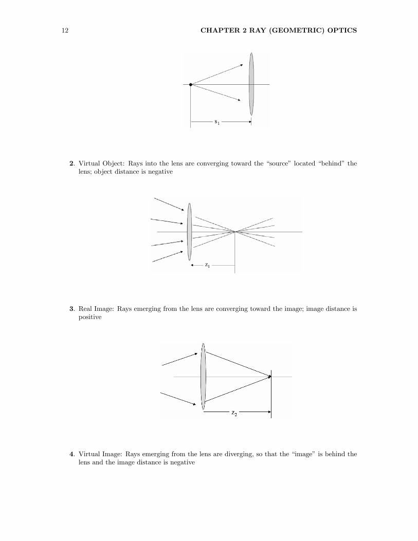
12 CHAPTER 2 RAY (GEOMETRIC) OPTICS
2. Virtual Object: Rays into the lens are converging toward the “source” located “behind” thelens; object distance is negative
3. Real Image: Rays emerging from the lens are converging toward the image; image distance ispositive
4. Virtual Image: Rays emerging from the lens are diverging, so that the “image” is behind thelens and the image distance is negative

2.5 HUMAN EYE 13
2.5 Human Eye
Since this course considers optics of imaging systems, and since the images generated by manyoptical systems are viewed by human eyes, we need to at least introduce the optics of the eye; wewill consider it in more detail when we trace rays through the “standard” eye model later.The optics of the human eye include the curved surface (the “cornea,” which exhibits most of
the power of the system) and a deformable lens. The system is intended to form an image on theretina, which is a fixed distance from the cornea. The lens is deformed by action of ciliary musclesto change the plane that is viewed “in focus.” When the muscles are relaxed, the lens is “flatter,”i.e., the radii of curvature of the surfaces are larger. To view an object “close up,” the focal lengthof the eye lens must be shortened by making the lens shape more spherical. This is accomplished bytightening the ciliary muscles (which is the reason why your eyes get tired after an extended timeof viewing objects up close).If the retina is located “too far” from the cornea, so that the image is “in front” of the retina
when the muscles are relaxed, then the eye sees a “blurry” image of distant objects, but nearbyobjects may be well focused. This is the condition of “nearsightedness” or “myopia.” If the retinais “too close” to the cornea, the image is focused behind it and the eye sees distant objects moresharply (“hyperopia” or “farsightedness.”)
2.6 Principle of Least Time
The mathematical model of ray optics is based on a principle stated by Fermat. Long before that,Hero of Alexandria hypothesized a model of light propagation that could be called the principle ofleast distance:
A ray of light traveling between two arbitrary points
traverses the shortest possible path in space. (Hero of Alexandria)
This statement applies to reflection and transmission through homogeneous media (i.e., the mediumis characterized by a single index of refraction). However, Hero’s principle is not valid if the objectand observation points are located in different media (as is the normal situation for refraction) or ifmultiple media are present between the points.In 1657, Pierre Fermat modified Hero’s statement to formulate the principle of least time (which
actually works):
A light ray travels the path that requires the least time to traverse. (Fermat)
The laws of reflection and refraction may be easily derived from Fermat’s principle. A moving ray

14 CHAPTER 2 RAY (GEOMETRIC) OPTICS
(or car, bullet, or baseball) traveling a distance s at a velocity v requires t seconds:
t =s
v
If the ray travels at different velocities for different increments of distance, the total travel time isthe summation over the different distances and different velocities:
t =MXm=1
smvm
If we define the velocity of a light ray in a medium of index n to be v =c
n. then:
t =MXm=1
sm³cnm
´ = 1
c
MXm=1
(nmsm) ≡c
where the optical path length is defined:
MXm=1
(nmsm) ≡
For a single medium, the optical path length is:
≡ n · s
Note that the optical path length is longer than the physical path length; it is the distance that aray would travel in vacuum in the same time that it would take to travel the physical distance s;the optical path is longer than the physical path because light travels more slowly in the medium(nm ≥ 1). The principle of least time may be restated as a light ray requires the least time totraverse the path with the shortest optical path length, or:
A ray traverses the route with the shortest optical path length.
This suggests a philosophical question, “How does the light ray know which path to take beforeit leaves the source?” I leave it to you to ponder this question, but will say that the difficulty ifformulating an answer suggests the limitation of the (simple) ray model for light propagation.
2.7 Fermat’s Principle for Reflection
Now consider the path traveled upon reflection that minimizes an easily evaluated optical pathlength:

2.7 FERMAT’S PRINCIPLE FOR REFLECTION 15
Schematic for determining the angle of reflection using Fermat’s principle.
As drawn, the angle θ1 is positive (measured from the normal to the ray) and θ2 is negative (from thenormal to the ray). The ray travels in the same medium of index n both before and after reflection.The components of the optical path length are:
so =ph2 + x2
op =
qb2 + (a− x)2
And the expression for the total optical path length is:
= n · (so+ op)
= n
µph2 + x2 +
qb2 + (a− x)
2
¶= [x] (a function of x)
By Fermat’s principle, the path length traveled is the minimum of the optical path length , so theposition of o along the x-axis is found by setting the derivative of with respect to x to zero:
d
dx=
d
dx
µn
µph2 + x2 +
qb2 + (a− x)
2
¶¶= 0
= n ·
⎛⎝ 2x
2√h2 + x2
+−2 (a− x)
2
qb2 + (a− x)2
⎞⎠=
x√h2 + x2
− a− xqb2 + (a− x)
2= 0
=⇒ x√h2 + x2
=a− xq
b2 + (a− x)2

16 CHAPTER 2 RAY (GEOMETRIC) OPTICS
From the drawing, note that:
sin [θ1] =x√
h2 + x2
sin [−θ2] =a− xq
b2 + (a− x)2
=⇒ sin [θ1] = sin [−θ2]=⇒ θ2 = −θ1
In words, the magnitudes of the angles of incidence and reflection are equal (as already derivedby evaluating Maxwell’s equations at the boundary). The negative sign is necessary because ofthe sign convention for the angle; the angle is measured from the normal and increases in thecounterclockwise direction, but the reversal of the propagation direction of the ray means that italso may be “explained” by assuming that the index of refraction for the image space is the negativeof that for the object space.
Snell’s law for reflection at interface.
Note that Snell’s law for reflection does not include either refractive index n, which means thatthe outgoing ray angle is not affected by the different refractive indices of the the two media, so theimage location and quality are not influenced by the indices. The “amount” of the ray that is reflectedIS affected by the two refractive indices via the Fresnel equations, which require the principles ofwave optics for explanation. At this point, we will just introduce the relationship without proof. Iflight is incident normally to the interface between two media (θ = 0) with refractive indices n1 andn2, the reflectivity of the surface obeys:
R =
µn1 − n2n1 + n2
¶2if θ = 0
If the first medium is air with n ' 1 and the second is glass with n ∼= 1.5, the reflectivity is:
R =
µ1− 1.51 + 1.5
¶2= 0.04
Note that the reflectivity is the same if the first medium is glass and the second is air:
R =
µ1.5− 11.5 + 1
¶2= 0.04
The reflectivity at different incident angles obeys more complicated expressions, in part because thelight must be decomposed into different polarizations depending on the direction of oscillation ofthe electric field.

2.7 FERMAT’S PRINCIPLE FOR REFLECTION 17
2.7.1 Plane Mirrors
Other than perhaps the pinhole, the simplest image forming system is the plane mirror, which isso familiar that it may seem hardly worth mentioning. Clearly its action obeys Snell’s reflectionlaw that θ2 = −θ1, which means that the the appearance of an image is “reversed” relative to theobject, i.e., the parity of the image is inverted. It also allows introduction of the concepts of objectspace and image space, which will be used thenceforth and forevermore. The object space is thelocus of points where objects may exist, which is all points “in front of” the mirror (real objects)and “behind” the mirror (virtual objects) . A real object forms a virtual image “behind” the mirror,and a virtual object forms a real image “in front of” the mirror. In other words, the object andimage spaces for reflection by a plane mirror both include the entire 3-D space.
Object and image space for a plane mirror. Rays diverging from a real object forms a virtual image“behind” the mirror, but rays converging to a virtual object “behind” the mirror form a real image
“in front of” the mirror.

18 CHAPTER 2 RAY (GEOMETRIC) OPTICS
2.8 Fermat’s Principle for Refraction:
Schematic for refraction using Fermat’s principle.
In this drawing, both θ1 and θ2 are positive (measured from the normal to the interface in thecounterclockwise direction). The optical path length is:
= n1 · so+ n2 · op
= n1ph2 + x2 + n2
qb2 + (a− x)2
By Fermat’s principle, the path length traveled is that such that is minimized, so we again set thederivative of with respect to x to zero and identify trigonometric functions for the resulting ratios.
d
dx= n1
2x
2√h2 + x2
+ n2−2 (a− x)
2qb2 + (a− x)2
= 0
=⇒ n1x√
h2 + x2= n2
a− xqb2 + (a− x)2
= 0
sin [θ1] =x√
h2 + x2
sin [θ2] =a− xq
b2 + (a− x)2
=⇒ n1 sin [θ1] = n2 sin [θ2]
=⇒ Snell’s Law for refraction
Note that with this sign convention, Snell’s law may be applied to reflection by setting the refractiveindex of the second medium to be the negative of the first:
n1 sin [θ1] = n2 sin [θ2]
=⇒ n1 sin [θ1] = −n1 sin [θ2]=⇒ − sin [θ1] = sin [θ2]=⇒ θ2 = −θ1

2.8 FERMAT’S PRINCIPLE FOR REFRACTION: 19
The expression of Snell’s law for refraction is general, but we can easily apply the first-order paraxialapproximation that sin [θ] ∼= θ if the ray angles are small (θn ∼= 0):
n1 sin [θ1] = n2 sin [θ2] =⇒ n1 · θ1 = n2 · θ2 in paraxial approximation=⇒ θ2 =
n1n2· θ1 in paraxial approximation
2.8.1 Dispersion
Unlike the reflection law, Snell’s law for refraction DOES include the refractive indices. This meansthat the angle of refraction will change as the indices change, as with wavelength. All (or perhapsI should day ALL) transparent materials exhibit a variation in refractive index with wavelength,which is called dispersion. Note that the features of dispersion depend on the material (e.g., glass).The full explanation of dispersion is beyond the scope of this course, so we will just describe itseffects.In a transparent matrial over the range of visible wavelengths, the refractive index n DE-
CREASES with increasing λ. In the study of wave optics, this ensures that the phase velocity
for the “average” wave vφ =ω
kis larger than the group or modulation velocity
dω
dk. Among other
things, this ensures that a signal transmitted as a modulation of a light wave cannot travel at aspeed faster than the velocity of light. A schematic dispersion for a hypothetical glass is shown inthe figure; note that the slope of the dispersion curve decreases with increasing λ; the curve “flattensout” as λ increases in the visible range.
Typical dispersion curve for glass at visible wavelengths, showing the decrease in n with increasingλ and the three spectral wavelengths specified by Fraunhofer and used to specify the “refractivity”,
“mean dispersion”, and “partial dispersion” of a material.
The refractive indices for several real glasses shows an additional feature of dispersion curves:the relationship between the “amount” of dispersion and the refractive index. Glasses with lowerrefractive index (n ∼= 1.5, the so-called crown glasses) have a “flatter” graph and therefore lessdispersion. In other words, nblue is larger than nred , but not much larger., so that the smaller therefractive index, the smaller the dispersion. Flint glasses have larger values of the refractive index(n ∼= 1.7) and larger variations across the visible spectrum:
(nblue − nred)fl int > (nblue − nred)crown

20 CHAPTER 2 RAY (GEOMETRIC) OPTICS
Dispersion curves for various optical glasses as a function of wavelength λ in the visible region ofthe spectrum (measured in Angstroms, where 1Å = 0.1 nm = 10−10m, 4000Å = 400nm) The rapidrise in the index at wavelengths in the ultraviolet region is due to the atomic resonances there.
If we use the paraxial approximation for rays in air entering a glass with refractive index n, theoutgoing ray angle θ2 is:
θ2 =1
n2· θ1 in paraxial approximation
Dispersion ensures that (n2)blue > (n2)red , which means that (θ2)blue < (θ2)red and the deviationangle δblue > δred .Since the outgoing ray angles are different for different colors, images will be formed at different
distances in different colors. This is the source of chromatic aberration in imaging systems.
Effect of dispersion on refraction: since the refractive index for red light is smaller, the angle ofrefraction measured from the normal is larger. Put another way, this means that the deviation
angle due to refraction is smaller for red light than for blue light.
In imaging, we often think of dispersion in refractive elements as an unfortunate “bug” in the

2.8 FERMAT’S PRINCIPLE FOR REFRACTION: 21
system, but you probably also know that it can be a very useful feature; it provides a tool forspreading white light into its constituent spectrum in a dispersing prism.
Dispersing prism with the two refractions, showing that the angle of deviation from the originalpath is larger for blue light than for red light.
From the figure, note that the angle of deviation of the ray from the original path is larger for bluelight due to the dispersion of light
δblue > δred for prism
The relationship between the wavelength and the deviation angle is complicated for refraction.As a side comment, note that light may also be dispersed into its spectrum by the phenomenon
of diffraction in gratings. However, the relationship between the wavelength and the deviation anglefor diffraction is very simple: the angle of deviation is proportional to the wavelength (for smallangles):
δ ∝ λ =⇒ δblue < δred for grating
This means that it is easier to construct an accurate spectrometer based on diffraction than basedon refractive dispersion.
2.8.2 Refractive Constants for Glasses
The refractive properties of glass are approximately specified by the refractivity and the measureddifferences in refractive index at the three Fraunhofer wavelengths F, D, and C:
Refractivity nD − 1 1.75 ≤ nD ≤ 1.5
Mean Dispersion nF − nC > 0 differences between blue and red indices
Partial Dispersion nD − nC > 0 differences between yellow and red indices
Abbé Number ν ≡ nD − 1nF − nC
ratio of refractivity and mean dispersion, 25 ≤ ν ≤ 65
(note that larger dispersions result in smaller Abbé numbers)Glasses are specified by six-digit numbers abcdef, where nD = 1.abc, to three decimal places,
and the Abbé number ν = de.f . Note that larger values of the refractivity mean that the refractiveindex is larger and thus so is the deviation angle in Snell’s law. A larger Abbé number means thatthe mean dispersion is smaller and thus there will be a smaller difference in the angles of refraction.Such glasses with larger Abbé numbers and smaller indices and less dispersion are crown glasses,while glasses with smaller Abbé numbers are flint glasses, which are “denser”. Examples of glassspecifications include Borosilicate crown glass (BSC), which has a specification number of 517645, soits refractive index in the D line is 1.517 and its Abbé number is ν = 64.5. The specification number

22 CHAPTER 2 RAY (GEOMETRIC) OPTICS
for a common flint glass is 619364, so nD = 1.619 (relatively large) and ν = 36.4 (smallish). Nowconsider the refractive indices in the three lines for two different glasses: “crown” (with a smaller n)and “flint:”
Line λ [ nm] n for Crown n for Flint
C 656.28 1.51418 1.69427
D 589.59 1.51666 1.70100
F 486.13 1.52225 1.71748
The glass specification numbers for the two glasses are evaluated to be:
For the crown glass:
refractivity: nD − 1 = 0.51666 ∼= 0.517
Abbé number : ν =1.51666− 1
1.52225− 1.51418∼= 64.0
Glass number = 517640
For the flint glass:
refractivity:L nD − 1 = 0.70100 ∼= 0.701
Abbé number : ν =0.70100− 1
1.71748− 1.69427∼= 30.2
Glass number = 701302
Dispersion curve of a material from very short to very long wavelengths. The index increases withincreasing λ as additional resonances are passed, but the index of refraction decreases with
increasing wavelength in the visible wavelengths (bold face).

2.8 FERMAT’S PRINCIPLE FOR REFRACTION: 23
The dispersion curves for optically transparent materials, such as glass and air, exhibit some verysimilar features, though the details may be significantly different. Starting at very short wavelengths(λ ' 0), the refractive index n is approximately unity. In words, the wavelength is so short (andthe oscillation frequency so large) that the energy per photon is very large, so that photons passthrough the material without interacting with the atoms; the material appears to be vacuum. Forlonger (but still very short) wavelengths (“hard” X rays), the refractive index actually is slightlyless than unity, which means that X rays incident on a prism are refracted away from the prism’sbase, rather than towards the base in the manner of visible light. This is the reason why X rays canbe totally reflected at grazing incidence, which is the focusing mechanism used in X-ray telescopes(such as Chandra). As the wavelength of the incident light increases further, though still within theX-ray region, the radiation incident on the material is heavily absorbed; this is the “K-absorptionedge” where the energy of the incident X rays is just sufficient to ionize an electron in the innermostatomic “shell” — the “K shell.” For example, the wavelength of this absorption is λK ∼= 0.67 nmfor silicon. Other absorptions occur at yet longer wavelengths (smaller incident photon energies),where electrons in the L and M shells, etc., of the atom are ionized. The spectrum of a materialwith a large atomic number (and thus several filled electron shells) will exhibit several such resonantabsorptions.
Ionization of a K-shell electron by an incoming X ray of sufficient energy. This is the reason forthe large absorptions of “hard” X rays by materials. Lower-energy (longer-wavelength) X rays will
ionize electrons in the L or M shells, thus producing other absorption “edges.”
As the wavelength of the incident radiation increases further, into the “far ultraviolet” region ofthe spectrum, the real part of the refractive index decreases to a value much less than unity withina wide band of anomalous dispersion. The fact that n < 1 in this region may be confusing becauseit seems that the velocity of light exceeds c, but these waves do not propagate in the material dueto the strong absorption (large value of κ). The wavelength of maximum absorption corresponds tothe largest of the several “natural oscillation frequencies” of bound electrons in the material.In the visible region of the spectrum, the dispersion curve exhibits the familiar decrease in n
with λ that was shown above. For example, the index of air is n ∼= 1.000279 at λ = 486.1 nm(Fraunhofer’s “F” line) and n ∼= 1.000276 at λ = 656.3 nm (“C” line). The corresponding values fordiamond are nF = 2.4354 and nC = 2.4100. The closer the nearest ultraviolet absorption to thevisible spectrum, the steeper will be the slope dn
dλ in the visible region and thus the larger the visibledispersion (defined below).The dispersion curve descends yet more steeply somewhere in the near infrared region and then
rises due to anomalous dispersion in the vicinity of an infrared absorption band (labeled “λ2” onthe graph). For quartz (crystalline SiO2), the center of this band is located at λ ∼= 8.5μm, but theabsorption already is quite strong for wavelengths as short as λ ∼= 4μm. Most optical materials haveseveral such infrared absorption bands and the “base level” of the index of refraction is larger aftereach such band. This behavior is confirmed by far-infrared measurements of the refractive index ofquartz (crystalline SiO2), which varies over the interval 2.40 ≤ n ≤ 2.14 for 51μm ≤ λ ≤ 63μm. Thelarge values of n ensure that the focal length of a convex quartz lens is much shorter at far-infrared

24 CHAPTER 2 RAY (GEOMETRIC) OPTICS
wavelengths than at visible wavelengths.As the wavelength is increased still further into the radio region of the spectrum after the last
absorption band, the refractive index decreases slowly due to normal dispersion from that last
absorption and approaches a limiting value ofr
0.
2.9 Image Formation in the Ray Model
We know that light rays are deviated at interfaces between media with different refractive indices.The goal in this section is to use interfaces of specified shapes to “collect” the light and “reshape”the wavefronts in a way that recreates “images” of the original sources.
2.9.1 Refraction at a Spherical Surface
Optical systems typically are used to form images of the source distribution by constructing opticalelements (“lenses”) made out of transparent media with different refractive indices to redirect theelectromagnetic radiation. Until rather recently, lenses were fabricated almost exclusively fromglass, which required the optical surfaces to be ground to the desired curvature and polished toremove scratches, etc., from the grinding. Two pieces of glass are typically employed in the grindingprocess: the “optic” and the “tool.” Water and a grinding compound composed of flecks of somehard substance resembling sand are placed on the surface of one glass and the two surfaces rubbedtogether with some force applied to the top optic. The two glass pieces are In the grinding process,The surface that is easiest to fabricate is a sphere, because the two surfaces will be in contactat all translations. Glass is ground out of the center of the top piece and off of the edges of thebottom piece, leaving a concave sphere on top and a convex sphere on the bottom. The “grit”of the grinding compound is reduced gradually to leave a smoother surface. The surface is thenpolished using very fine “jeweler’s rouge” to produce smooth surfaces of “optical” quality. Morerecently, optical elements have been fabricated from thin plates cemented over a hollowed-out “grid”to lighten the weight. Also plastics and other materials have been developed that may be cast toproduce optical surfaces of various shapes with minimal polishing.
Grinding optical surfaces: a slurry of water and grinding compound (e.g., carborundum) is placedbetween two glass surfaces. The top glass is pushed down and moved around to grind glass from thecenter region of the top piece. The resulting surfaces must be spherical because they are the only
curves that remain in contact at all locations.
Consider the action of a spherical surface of a medium with index n2 on an incident ray in amedium of index n1:

2.9 IMAGE FORMATION IN THE RAY MODEL 25
Refraction at a spherical surface between two media of refractive index n1 and n2.
The point source is located at s and its distance to the vertex v is sv ≡ z1 > 0. The distancefrom vertex v to the observation point p is vp ≡ z2 > 0. The physical distance traveled by a ray inmedium n1 to the surface is sa ≡ 1 and that in medium n2 is ap ≡ 2. The radius of curvature ofthe surface is vc = ac ≡ R > 0 as drawn. For emphasis, we repeat that z1, z2, and R are all positivein our convention. The ray intersects the surface at angle ϕ (the “position angle”) measured fromthe center of curvature c. The optical path length of the ray from s to p through a is
OPL = n1 1 + n2 2 = n1 (sa) + n2 (ap)
The triangles 4sac and 4acp has sides 1 and R with hypotenuse z1+R, while 4acp has sidesR and z2 −R, with hypotenuse ap ≡ 2. The physical lengths 1 and 2 may be evaluated from theother two sides and the included angle ϕ via the law of cosines:
4sac =⇒ 21 = (z1 +R)
2+R2 − 2R (z1 +R) cos [ϕ]
=⇒ 1 =
q(z1 +R)
2+R2 − 2R (z1 +R) cos [ϕ]
4acp =⇒ 22 = (z2 −R)2 +R2 − 2R (z2 −R) cos [π − ϕ]
=⇒ 2 =
q(z2 −R)2 +R2 + 2R (z2 −R) cos [ϕ]
=
q(z2 −R)2 +R2 − 2R (R− z2) cos [ϕ]
The corresponding optical path length is:
OPL = n1 1 + n2 2
= n1 ·µq
(z1 +R)2+R2 − 2R (R+ z1) cos [ϕ]
¶+ n2 ·
µq(z2 −R)
2+R2 − 2R (R− z2) cos [ϕ]
¶which is obviously a function of the position angle ϕ. We can now apply Fermat’s principle to find

26 CHAPTER 2 RAY (GEOMETRIC) OPTICS
the angle ϕ for which the OPL is a minimum:
d
dϕ(OPL) = 0
=n1 · 2R (R+ z1) sin [ϕ]q
(z1 +R)2+R2 − 2R (R+ z1) cos [ϕ]
+n2 · 2R (R− z2) sin [ϕ]q
(z2 −R)2+R2 − 2R (R− z2) cos [ϕ]
= 2R sin [ϕ]
µn1 (R+ z1)
1+
n2 (R− z2)
2
¶which may be rearranged to:
0 = 2R sin [ϕ]
µn1 (R+ z1)
1+
n2 (R− z2)
2
¶=⇒ 0 =
n1 (R+ z1)
1+
n2 (R− z2)
2
=⇒ n1R
1+
n2R
2=
n2z2
2− n1z1
1
=⇒ n1
1+
n2
2=1
R
µn2z2
2− n1z1
1
¶This last relation between the physical path lengths 1 and 2 and the distances z1 and z2 is exact.Now we use the expression for the physical path length 1 to find its ratio relative to the axialdistance z1 and use simple algebra to rearrange:
1
z1=
q(z1 +R)2 +R2 − 2R (z1 +R) cos [ϕ]
z1
=
Ã(z1 +R)
2+R2 − 2R (z1 +R) cos [ϕ]
z21
! 12
=
µz21 +R2 + 2Rz1 +R2 − 2R2 cos [ϕ]− 2Rz1 cos [ϕ]
z21
¶ 12
1
z1=
µ1 +
µ2R2
z21+2R
z1
¶(1− cos [ϕ])
¶ 12
This relation also is exact, but may be approximated by applying a truncated series for cos [ϕ]:
cos [ϕ] = 1− ϕ2
2!+
ϕ4
4!− ϕ6
6!+ · · · ∼= 1 if ϕ ∼= 0
=⇒ 1− cos [ϕ] = 1−µ1− ϕ2
2!+
ϕ4
4!− ϕ6
6!+ · · ·
¶=
ϕ2
2!− ϕ4
4!+
ϕ6
6!− · · ·
∼= 0 if ϕ ∼= 0
This leads to the first-order approximation that the path length and axial length are approximatelyequal:
1
z1∼= 1 =⇒ 1
∼= z1

2.9 IMAGE FORMATION IN THE RAY MODEL 27
Similarly, we can show that:2∼= z2
This paraxial or Gaussian approximation (also called first-order optics because it is based on onlythe first-order term in the cosine series) is valid only for small ray angles ϕ measured from the opticalaxis. In words, the optical path lengths of rays that travel along the optical axis and rays that travel“away” from the axis (but still with ϕ ∼= 0) are equal.The simplified imaging equation has the form:
1
R
µn2z2
2− n1z1
1
¶∼=1
R(n2 − n1)
=⇒ n1z1+
n2z2∼=1
R(n2 − n1)
This is the paraxial imaging equation for single surface; clearly it is an approximation to the trueequation, and also clearly it is similar to the imaging equation we have already considered.
Object at Infinite Distance
Now consider some pairs of object and image distances z1 and z2. If the object is located at −∞,then:
n1∞ +
n2z2=
n2z2∼=1
R(n2 − n1)
=⇒ z2 ∼=n2R
n2 − n1≡ f2 the “image-space focal length”
which is what we “normally” think of as being the focal length of the optic.
Image at Infinite Distance
If the image is located at +∞, the object distance must be
n1z1∼=1
R(n2 − n1) =⇒ z1 ∼=
n1R
n2 − n1≡ f1 the “object-space focal length”
1
f1=1
R(n2 − n1)
Also note that:
f1f2=
µn1R
n2 − n1
¶µ
n2R
n2 − n1
¶ =n1n2
=⇒ n1 · f2 = n2 · f1
In words, the ratio of the focal lengths in the two spaces (object and image) is the ratio of the indicesof refraction in the two spaces.Rule of Thumb: Estimating focal lengths of converging lenses: For a single positive
(converging) lens (i.e., not a lens “system” with multiple elements), it is easy to estimate the focallength of a lens by finding the distance from the lens to the image of a distant bright object. Therequirement for “distant” is not critical — forming the image of ceiling lamp on the floor or a tabletopwill give a useful estimate for a positive lens with a short focal length.
2.9.2 Imaging with Spherical Mirrors
The equation for a single refractive surface may be used to derive the focal length of a sphericalmirror by setting the refractive index of image space to the negative of that in object space:

28 CHAPTER 2 RAY (GEOMETRIC) OPTICS
φ =1
f=1
R(−n1 − n1) = −2
n1R
In air, the equation for the focal length of a spherical mirror is:
f = − R
2n→ −R
2in air
In words, the focal length of a spherical mirror is half of the radius of curvature; the focal length ispositive (converging) if R > 0 and negative if R < 0, as shown.
Spherical mirrors: concave mirror with negative radius of curvature R = VC < 0 makes outgoinglight rays converge and so f > 0; convex mirror with positive radius of curvature makes rays diverge
and f < 0.
2.10 First-Order Imaging with Thin Lenses
Normally we do not consider the case of an object in one medium with the image in another — usuallyboth object and image are in air and a lens (a “device” composed of material with different refractiveindex n and curved surfaces) diverts the rays to form the image. We can derive the formula for theobject and image distances if we know the radii of the lens surfaces and the indices of refraction.We merely cascade the formula for a single surface:
At first surface:n1z1+
n2z01=
n2 − n1R1
At second surface:n2z2+
n3z02=
n3 − n2R2
where z1 is the (usually known) object distance, z01 is the image distance for rays refracted by thefirst surface, z2 is the object distance for the second surface, and z02 is the image distance for raysexiting the second surface (and thus from the lens). For the common “convex-convex” lens, the

2.10 FIRST-ORDER IMAGING WITH THIN LENSES 29
center of curvature of the first surface is to the right of the vertex, and thus the radius R1 of thefirst surface is positive. Since the vertex is to the right of the center of curvature of the secondsurface, then R2 < 0. If the lens is “thin”, then the ray encounters the second surface immediatelyafter refraction at the first surface, so the ray heights at the two surfaces are the same. The objectdistance for the second surface is the negated image distance from the first: z2 = −z01. Put anotherway, the absolute value of the image distance for the front surface |z01| is the same as the objectdistance for the second surface |z2|. If the lens is “thick”, then the object distance for the secondlens is different from the image distance for the first, and the ray heights will be different if the rayangle is not zero. The thickness t of the lens must satisfy the relationship:
z01 + z2 = t =⇒ z2 = t− z01 for thick lens
for a thick lens. For a thin lens with t = 0
z2 = 0− z01 =⇒ z2 = −z01 for thin lens
The equations for the two surfaces may be added and the RHS may be rearranged to obtain asingle imaging equation for a lens with two surfaces:µ
n1z1+
n2z01
¶+
µn2z2+
n3z02
¶=
µn2 − n1R1
¶+
µn3 − n2R2
¶=
n3R2
+ n2
µ1
R1− 1
R2
¶− n1
R1
For a thin lens with t = 0, substitute z2 = −z01 to obtain:
t = 0 =⇒ n1z1+
n3z02=
µn1z1+
n2−z2
¶+
µn2z2+
n3z02
¶n1z1+
n3z02
=n3R2
+ n2
µ1
R1− 1
R2
¶− n1
R1
where the object is immersed in index n1, the lens has index n2, and the image is immersed in indexn3.
In the usual case of both object and image in air so that n3 = n1 = 1,the equation simplifies to:
1
z1+1
z02=
1
R2+ n2
µ1
R1− 1
R2
¶− 1
R1
1
z1+1
z02= (n2 − 1)
µ1
R1− 1
R2
¶Note the similarity between this equation and that we inferred from the derivation of the imageplane using wave optics:
1
z1+1
z2=1
f
where the distances z1 and z2 from the object to the lens and lens to image are what we had calledz1 and z2 previously, and we identify:
(n2 − 1)µ1
R1− 1
R2
¶=1
f=1
z1+1
z02(Lensmaker’s Equation)
which defines the focal length of the thin lens in terms of its physical parameters for a thin lens.This is the so-called lensmaker’s equation for thin lenses IN AIR; it determines the distance z02 tothe image for object distance z1, the radii of curvatures R1 and R2 of the spherical surfaces, and the

30 CHAPTER 2 RAY (GEOMETRIC) OPTICS
index of refraction n2 of the glass. Note that the object distance z1 and the image distance z02 bothappear with the same algebraic sign, which may be interpreted as demonstrating an “equivalence”of the object and image because the propagation of light rays may be reversed to exchange the rolesof object and image. Corresponding object and image points (or object and image lines or objectand image planes) are called conjugate points (or lines or planes).In the more general case where the refractive index of object space is n3 > 1 so that n3 6= n1,
the focal length of the lens is:
(n2 − 1)µn1R1− n3
R2
¶=1
f
and that of image space is n3.
2.10.1 Examples of Thin Lenses
1. Plano-convex lens, curved side forward (“convexo-planar lens”)
R1 = |R1| > 0R2 = ±∞ (sign has no effect)
1
z1+1
z02= (n2 − 1)
µ1
|R1|− 1
∞
¶=
n2 − 1|R1|
> 0
If z1 = +∞, then z02 = f > 0, the focal length1
f=
n2 − 1R1
= φ system power (measured in meters−1 = diopters)
f =R1
n2 − 1∼= 2R1 (since n2 ∼= 1.5 for glass)
We often use the “power” φ = f−1 (measured in m−1 = diopters) instead of the focal lengthf to describe the lens, since powers of different lenses combine by addition, instead of asreciprocals of sums of reciprocals. The power measures the ability of the lens or lens systemto deviate rays, i.e., to change the ray angle.
2. Plano-convex lens, plane side forward:
R1 = ±∞R2 = − |R2| < 0
1
z1+1
z02= −(n2 − 1)
R2= +
(n2 − 1)|R2|
> 0
f =|R2|n2 − 1
∼= 2 |R2|
So the focal length of the lens is the same regardless of its orientation (front-to-back). Sincethe focal lengths for the two configurations (curved side in front or behind lens) are the same,you might assume that the same image quality can be expected for the two configurations.This is NOT the case, but the explanation requires the theory of aberrations. At this point,we will just try to give a bit of motivation for another rule of thumb, while postponing theproof.
Rule of Thumb: Orientation of Plano-Convex Lens: When using a plano-convex lensto form an image, the quality of the image is better if the power is more evenly divided amongthe two surfaces. This means that the the curved side of the lens is placed towards the longerconjugate (which usually is towards the object) and the plane side towards the shorter conju-gate. This miniizes the spherical aberration that causes rays from a point object to cross theoptical axis at different distances from the lens. This perhaps may be visualized better if weconsider the case of a distant object (assume z1 = ∞) and a plano-convex lens with the flat

2.10 FIRST-ORDER IMAGING WITH THIN LENSES 31
side towards the object. For an object at infinity, the rays incident upon the lens are parallel(“collimated”) both when they are incident to and when they exit the flat surface. In otherwords, the flat side contributes no power to the imaging, so all of the focusing power comesfrom the curved surface.
Rule of thumb: when using a plano-convex lens, place the curved side towards the longer conjugateto get a better image.
3. Plano-concave, plane side forward:
R1 = ±∞R2 = + |R2| > 0
1
z1+1
z02= (n2 − 1)
µ1
∞ −1
+ |R2|
¶= − (n2 − 1)|R2|
< 0
f = − |R2|n2 − 1
∼= −2 |R2|
4. Double convex lens with equal radii:
R1 = |R| > 0R2 = −R1 = − |R|
1
z1+1
z02= (n2 − 1)
µ1
|R| −µ− 1
|R|
¶¶= 2
(n2 − 1)|R| > 0
1
f= φ =
2 · (n2 − 1)|R|
f =|R|
2 · (n2 − 1)∼= |R| > 0 if n2 ∼= 1.5

32 CHAPTER 2 RAY (GEOMETRIC) OPTICS
2.10.2 Spherical Mirror
The mirror changes the direction of rays by reflection that obeys Snell’s law for reflection so thatthe angle of reflection is the negative of the angle of incidence (measured from the normal to thesurface). For a concave spherical mirror, the incident ray angle varies with height above the opticalaxis. difference in analysis between the single refractive surface and the mirror may be simplified byrecognizing that the mirror “reverses” the direction of propagaion of light, which may be explainedby setting n2 = −n1 = −1
1
f=1
R− −1
R= − 2
R=⇒ f = −R
2
In words, the focal length of a spherical mirror is half of the radius of curvature. A concave mirrorwith negative radius is positive (center to left of vertex)
2.11 Image Magnifications
The most common use for a lens is to change the apparent size of an object (or image) via themagnifying properties of the lens. The mapping of object space to image space “distorts” the sizeand shape of the image, i.e., some regions of the image are larger and some are smaller than theoriginal object. We can define three types of magnification: transverse, longitudinal, and angular,where the first two describe the impact of the imaging system on lengths that are respectivelyperpendicular to and parallel to the optical axis, while the last refers to the action on the anglesof rays measured from the optical axis. Note that the very name of “magnification” is rathermisleading because most imaging systems produce images that are smaller than the object; theyactually “minify” the features because the magnifications are smaller than unity.
2.11.1 Transverse Magnification:
The transverse magnification MT is what we usually think of as magnification — it is the ratio ofobject to image dimension measured transverse to the optical axis. In the figure, note the two similartriangles 4a1b1c and 4a2b2c:
The transverse magnification of the image is the ratio of the height of the image to that of theobject: MT =
y2y1.
It is easy to see that:
y1z1=|y2|z2
= −y2z2(because y2 < 0)
=⇒ y2y1≡MT = −
z2z1
If |MT | is larger than or smaller than unity, the image is magnified or minified, respectively. IfMT > 0, the image is upright or erect and if MT < 0, the image is inverted (“upside down”).

2.11 IMAGE MAGNIFICATIONS 33
2.11.2 Longitudinal Magnification:
The longitudinal magnification ML is the ratio of the “length” or “depth” of the image measuredalong the optical axis to the corresponding length of the object; the longitudinal magnification isthe ratio of differential elements of length of the image and object, which approach an infinitesimalin the limit:
ML =∆z2∆z1
lim∆z1→0
∆z2∆z1
=dz2dz1
The expression may be derived by evaluating the total derivative of the lensmaker’s equation.
1
z1+1
z2= (n− 1)
µ1
R 1− 1
R2
¶Since the imaging equation relates the reciprocal distances z−11 and z−12 , the longitudinal magnifica-tion varies for different object distances. The total derivative of the left-hand side of the imagingequation is:
d
µ1
z1+1
z2
¶= d
µ1
z1
¶+ d
µ1
z2
¶= − 1
z21dz1 −
1
z22dz2
The derivative of the right-hand side is:
d
µ(n− 1)
µ1
R 1− 1
R2
¶¶= (n− 1) · d
∙µ1
R 1− 1
R2
¶¸= 0 (because n,R1, and R2 are constants)
We combine these to see that:
− 1z21dz1 −
1
z22dz2 = 0 =⇒ − 1
z21dz1 =
1
z22dz2
=⇒ dz2dz1
= −µz2z1
¶2We can now identify the ratio of the two differential lengths along the axis as the longitudinalmagnification ML:
ML ≡dz2dz1
= −µz2z1
¶2= − (MT )
2 < 0
The longitudinal magnification is negative because the image moves away from the lens (increasingz2) as the object moves towards the lens (decreasing z1). The longitudinal magnification affects theirradiance of the image (i.e., the “flux density” of the rays at the image); if |ML| is large, then thelight in the vicinity of an on-axis location is “spread out” over a longer longitudinal dimension atthe image, which requires the irradiance of the image to decrease.
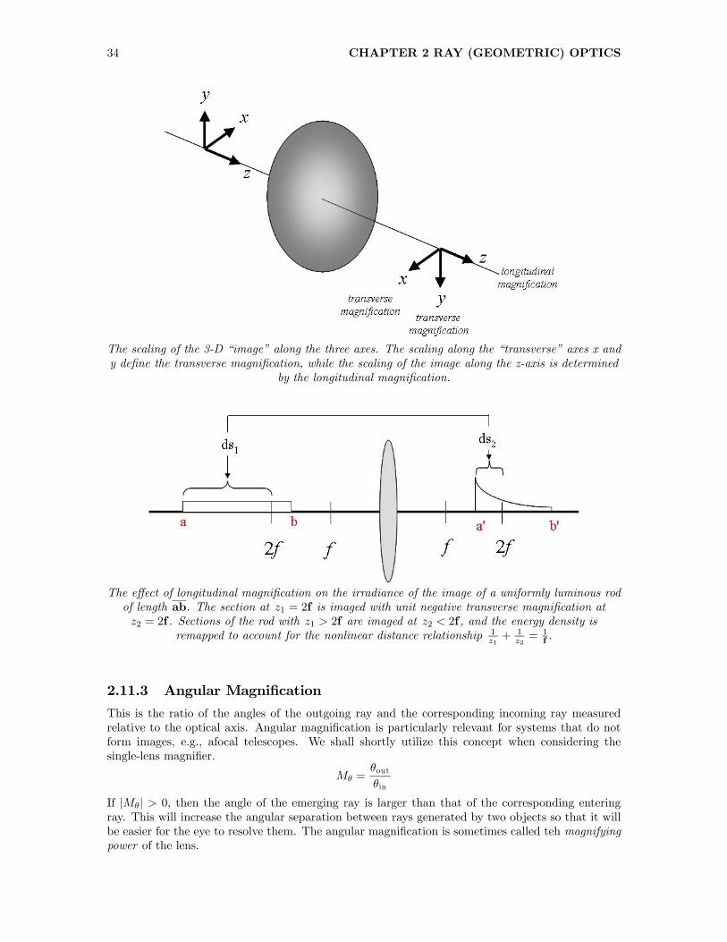
34 CHAPTER 2 RAY (GEOMETRIC) OPTICS
The scaling of the 3-D “image” along the three axes. The scaling along the “transverse” axes x andy define the transverse magnification, while the scaling of the image along the z-axis is determined
by the longitudinal magnification.
The effect of longitudinal magnification on the irradiance of the image of a uniformly luminous rodof length ab. The section at z1 = 2f is imaged with unit negative transverse magnification atz2 = 2f . Sections of the rod with z1 > 2f are imaged at z2 < 2f , and the energy density is
remapped to account for the nonlinear distance relationship 1z1+ 1
z2= 1
f .
2.11.3 Angular Magnification
This is the ratio of the angles of the outgoing ray and the corresponding incoming ray measuredrelative to the optical axis. Angular magnification is particularly relevant for systems that do notform images, e.g., afocal telescopes. We shall shortly utilize this concept when considering thesingle-lens magnifier.
Mθ =θoutθin
If |Mθ| > 0, then the angle of the emerging ray is larger than that of the corresponding enteringray. This will increase the angular separation between rays generated by two objects so that it willbe easier for the eye to resolve them. The angular magnification is sometimes called teh magnifyingpower of the lens.

2.12 SINGLE THIN LENSES 35
2.12 Single Thin Lenses
2.12.1 Positive Lens
The power of a single lens with two surfaces is determined by the lensmaker’s equation:
φ =1
f= φ1 + φ2 = (n2 − 1)
µ1
R1− 1
R2
¶The power is positive if 0 < R1 < |R2|. The most common case is the “double convex” lens
where R1 > 0, R2 < 0, which means that the ray encounters positive power at both surfaces. Theaction of a single thin positive lens with known focal length on an object with known location maybe solved graphically by sketching three specific rays from the tip of the object:
1. the ray parallel to the optical axis; this ray is refracted by the lens to pass through the image-space focal point F,
2. the ray through the center of the lens, which is not refracted by the thin lens and so maintainsthe same angle relative to the optical axis, and
3. the ray through the object-space focal point F0 to the lens; this ray is refracted and travelsparallel to the optical axis.
The intersection of these three rays (or obviously of any two) is the location of the image ofthe tip of the object:
The example in the figure closely matches the situation where the image is an inverted replica ofthe object, so that h0 = −h and MT = −1. The two equations that must be satisfied are
z2 = z1 =⇒ MT = −11
z1+1
z2=1
f=⇒ z1 = z2 = 2 · f
This situation where the object and image distances are twice the focal length is often called imagingat equal conjugates.This drawing assumes that the indices of refraction in object and image space are identical. If the
indices are different (e.g., if the object is in water and the image in air), then the imaging equation

36 CHAPTER 2 RAY (GEOMETRIC) OPTICS
must be modified:
φ =n− n1R1
− n2 − 1R2
=n1z1+
n2z2
If the refractive indices in object and image spaces are larger than that of the lens, such as acase where the object and image are in glass or water and the lens is “made of” air, the curvaturesmust be reversed, so that R1 < 0 and R2 > 0 to make a positive lens.
Lens made of rare medium (e.g., air) within a dense medium (e.g., glass, water). The reversal ofrefractive indices requires inverting of the signs of the radii of curvature.
2.12.2 Negative Lens
A lens with negative power at both surfaces may be constructed if R1 is negative and R2 is positive.Two (or more) rays that have passed through a lens with negative power will exhibit a largerdiivergence on the output side than on the input side.
2.12.3 Meniscus Lenses
A lens with radii of curvature with the same sign on both surfaces is a meniscus lens. If both radiiare positive, then the powers of the two surfaces are:
φ1 =n− 1|R1|
+1− n
|R2|= (n− 1) ·
µ1
|R1|− 1
|R2|
¶which may be positive or negative depending on the relative sizes of R1 and R2; the power is positiveif R2 > R1 and negative if R2 < R. An example of a meniscus lens with positive power is shown inthe figure.
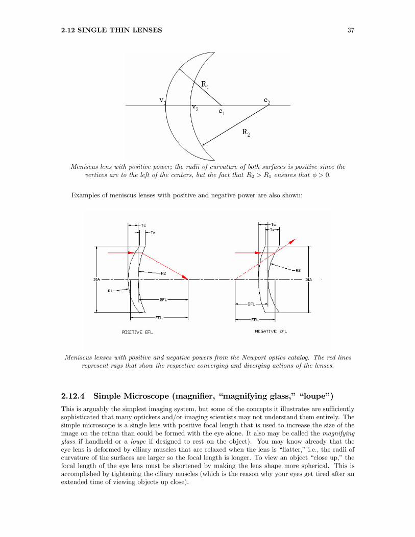
2.12 SINGLE THIN LENSES 37
Meniscus lens with positive power; the radii of curvature of both surfaces is positive since thevertices are to the left of the centers, but the fact that R2 > R1 ensures that φ > 0.
Examples of meniscus lenses with positive and negative power are also shown:
Meniscus lenses with positive and negative powers from the Newport optics catalog. The red linesrepresent rays that show the respective converging and diverging actions of the lenses.
2.12.4 Simple Microscope (magnifier, “magnifying glass,” “loupe”)
This is arguably the simplest imaging system, but some of the concepts it illustrates are sufficientlysophisticated that many optickers and/or imaging scientists may not understand them entirely. Thesimple microscope is a single lens with positive focal length that is used to increase the size of theimage on the retina than could be formed with the eye alone. It also may be called the magnifyingglass if handheld or a loupe if designed to rest on the object). You may know already that theeye lens is deformed by ciliary muscles that are relaxed when the lens is “flatter,” i.e., the radii ofcurvature of the surfaces are larger so the focal length is longer. To view an object “close up,” thefocal length of the eye lens must be shortened by making the lens shape more spherical. This isaccomplished by tightening the ciliary muscles (which is the reason why your eyes get tired after anextended time of viewing objects up close).

38 CHAPTER 2 RAY (GEOMETRIC) OPTICS
The closest distance to an object that appears to be sharply focused by the unaided eye is thenear point, which (obviously) depends on the flexibility of the deformable eyelens and the capabilityof the ciliary muscles, which (obviously) vary with individual, and with age for a single individual.The distance to the near point may be as close as 50mm ∼= 2 in for a young child and in the rangebetween 1000mm − 2000mm for an elderly person. This reduction in “accommodation” for closeobjects is one of the signs of aging. The near point of an “ideal” eye is assumed to be 250mm ∼= 10 infrom the front surface. For nearsighted individuals, the near point is closer to the eye, thus increasingthe angular subtense of fine details for those individuals. For this reason, nearsighted individualsin ancient times (before optical correction) often were attracted to professions requiring fine work,such as goldsmithing. Since nearsightedness can be a genetic trait, descendents often continued inthese crafts.
The reference for angular magnification is the angle subtended by the object if viewed at thenear point of the average eye so that z1 = 250mm. If the object height is y, the angle when viewedat the near point is:
θ250mm = tan−1h y
250mm
i∼=
y
250mm
where the first-order approximation tan [θ] ∼= θ if θ ∼= 0 is used in the last step.
Magnifier with Object at Focal Point of Positive Lens
If the object is positioned at the object-space (front) focal point of a positive lens with focal lengthflens , then the arays from the “tip” of the object are parallel when they exit the lens and so may beviewed “in focus” by an eye with a relaxed lens for an object at an infinite distance away. The anglesubtended by the object one focal length away is:
θlens = tan−1∙
y
flens
¸∼=
y
flens

2.12 SINGLE THIN LENSES 39
Magnifier with object at focal point of lens. Figure (a) at top shows the angle θ250mm subtended bythe object when located at the near point; (b) shows the angle θlens subtended by the object whenlocated at the object-space focal point of the lens. The blue ray in (b) emerges parallel to the optic
axis, which shows that the object distance z1 = f .
The angular magnification ormagnifying power of the magnifier is the ratio of the angle subtendedby the object when viewed at the closer distance through the lens to the angular subtense viewedat the near point:
Mθ =θlens
θ250mm=
tan−1∙
y
flens
¸tan−1
h y
250mm
i ∼=µ
y
flens
¶³ y
250mm
´Mθ =
250mm
flens, object at focal point
If the focal length of the magnifying lens is, say f = 50mm, then the magnifying power of the lensfor the object at the focal point is:
Mθ =250mm
50mm= 5
Magnifier with Image Formed at Near Point
We can instead use the magnifying lens held close to the eye to form a virtual image at the nearpoint of the eye. This means that the distance from the lens to the virtual image formed by the lensis the distance to the near point: V0O0 = z2 = −250mm. ISubstitute this distance into the imaging

40 CHAPTER 2 RAY (GEOMETRIC) OPTICS
equation:
1
z1+
1
−250mm =1
f
=⇒ 1
z1=1
f+
1
250mm=⇒ z1 =
250mm · f250mm+ f
The angle subtended by the object at the near point is the same as before:
θ250mm = tan−1h y1250mm
i∼=
y1250mm
but the angle subtended by the image when positioned at the near point viewed through the lens isdifferent:
θlens = tan−1∙
y2|−250mm|
¸∼=
y2250mm
=y1z1
where the similarity of the triangles has been used. This expression may be recast by substitutingthe expression for z1:
θlens ∼=y1z1=
y1µ250mm · f250mm+ f
¶ =y1f·µ250mm+ f
250mm
¶
The magnifying power is:
Mθ =θlens
θ250mm=
³y1f
´·µ250mm+ f
250mm
¶³ y1250mm
´ =250mm+ f
f
Mθ =250mm
flens+ 1 image at near point
Magnifier with image at near point of eye. The top figure again shows the angle θ250mm subtendedby the object when located at the near point. The second figure shows the image at the near point,
which is more distant than the object.

2.13 SYSTEMS OF THIN LENSES 41
2.13 Systems of Thin LensesThe images produced by systems of thin lenses may be located by finding the “intermediate” imageproduced by the first lens, which then become in turn the objects for the second lens, which generatesan image that is the object for the third lens, etc. This type of analysis also may be applieddirectly to the more realistic case of “thick” lenses, where the first “lens” actually represents thefirst surface of the thick lens and the light propagates through the glass between the surfaces.Though straightforward, this “sequential” solution to the image may be tedious and also not veryilluminating (pun intended) about the action of the system of lenses. The object and distance forthe nth lens will be denoted by zn and the corresponding image distance by the primed quantity z0n.
2.13.1 Two-Lens System
Consider a two-lens system with first lens L1 and second lens L2 separated by the distance t. Theobject for the system shown in the figure is labelled by O and the corresponding image by O0, theobject- and image-space focal points are F and F0, and the object- and image-space vertices (firstand last surfaces of the system) by V and V0.
Imaging by a system of two thin lenses L1 and L2 separated by the distance t. The object andimage distances for the first lens are z1 and z01 and for the second lens are z2 and z02.
From the diagram, we see that z01 the image distance from the first lens, z2 the object distance forthe second lens, and the lens separation t are related by:
z01 + z2 = t
so the object distance for the second lens is z2 = t − z01. The imaging equation for the first lensdetermines z01:
1
z1+1
z01=1
f1=⇒ 1
z01=1
f1− 1
z1=
z1 − f1z1f1
=⇒ z01 =z1f1
z1 − f1If z1 =∞, then the
z01 = limz1→∞
z1f1z1 − f1
= f1 · limz1→∞
µz1
z1 − f1
¶= f1 · 1 = f1

42 CHAPTER 2 RAY (GEOMETRIC) OPTICS
In words, the image distance from the first lens for an object at ∞ is the focal length of the firstlens, as it should be. The object distance to the second lens is z2 = t− z01, which may be rewrittenin terms of z1, f1, and t for the general case:
z2 = t− z01 = t− z1f1z1 − f1
=z1t− f1t− z1f1
z1 − f1
=z1 (t− f1)− f1t
z1 − f1In the limit of infinite object distance, the object distance to the second lens is:
z2 [for z1 =∞] = limz1→∞
µz1
z1 − f1· (t− f1)−
f1t
z1 − f1
¶= 1 · (t− f1)− 0= t− f1
which is the difference in the separation of the lenses and the distance from the image-space focalpoint of the first lens; this often is a negative distance (i.e., virtual object for the second lens).
In the general case, apply the imaging equation for the second lens and substitute for the ex-pression for z2:
1
z02=
1
f2− 1
z2
=1
f2− z1 − f1
z1 (t− f1)− f1t
1
z02=
t− z1(z1 − f1)
(f1 + f2) +f1f2
(z1 − f1)f2 · t− f1 · f2 ·
z1(z1 − f1)
=⇒ z02 =
f2 · t− f1 · f2 ·z1
(z1 − f1)
t− z1(z1 − f1)
(f1 + f2) +f1f2
(z1 − f1)
=
f2 ·µt− f1 · z1
(z1 − f1)
¶t− z1 · (f1 + f2)− f1f2
(z1 − f1)
The image distance for a specified (non-infinite) object location is called the back focal distance bysome authors:
BFD = z02 = V0O0 =
f2 ·µt− f1 · z1
(z1 − f1)
¶t− z1 · (f1 + f2)− f1f2
(z1 − f1)

2.13 SYSTEMS OF THIN LENSES 43
In the limit of infinite object distance, the BFD becomes the back focal length BFL:
limz1→∞
[z02] = z02 [f1, f2, t; z1 =∞] ≡ V0F0
= limz1→∞
⎛⎜⎜⎝ f2 ·µt− f1 ·
z1(z1 − f1)
¶t− z1 · (f1 + f2)− f1f2
(z1 − f1)
⎞⎟⎟⎠=
f2 · (t− f1 · 1)t− 1 · (f1 + f2)− 0 · f1f2
=t · f2 − f1f2t− (f1 + f2)
=f1 · f2 − f2 · t(f1 + f2)− t
BFL = V0F0 =f1 · f2 − f2 · t(f1 + f2)− t
=(f1 − t) · f2(f1 + f2)− t
These complicated expressions, for the image distances measured from the second lens in terms ofthe two focal lengths f1 and f2, the separation t, and the distance z1 from the object to the firstlens, are useful, but it tell little on its face about the entire “lens system.” We would much preferestablishing relationships from the object to the lens system and from the system to the image. Thefirst step in this analysis is to define an equivalent or effective focal length for the entire system,which is the focal length of the equivalent single thin lens.
2.13.2 Effective (Equivalent) Focal Length
We can use the results just derived to find an expression for the imaging action of a two-lens systemby finding the location and focal length of the equivalent single lens that would generate the sameimage. This is an important concept, so we will do a rigorous derivation, which is perhaps simplifiedby adding some details to the figure:
Ray diagram of system of two positive thin lenses to illustrate the concept of “effective” (or“equivalent”) focal length feff , back focal length BFL = z02 = V
0F0, and principal point H0
The continuations of the input outgoing rays intersect at B, whose projection onto the optical axisis at H0, this is the location of the equivalent single lens that would generate the same outgoingray from the incoming ray. The distance from H0, the image-space principal point, to F0 is theimage-space effective (or equivalent) focal length:
H0F0 ≡ feff

44 CHAPTER 2 RAY (GEOMETRIC) OPTICS
We have already evaluated the back focal length, which is the image location for an object at infinity:
V0F0 = z02 [z1 =∞] =(f1 − t) · f2(f1 + f2)− t
Compare two sets of similar triangles: ∆¡AVF01
¢∼ ∆
¡CV0F01
¢and ∆
¡BH0F0
¢∼ ∆
¡CV0F0
¢shown in the figures:
From the first pair of triangles ∆¡AVF01
¢∼ ∆
¡CV0F01
¢, we can construct ratios of their
“heights” and “axial lengths:”
h1
VF01=
h2
V0F01=⇒ h2
h1=V0F01
VF01
Now note that the distance VF01 = f1, while V0F01 may be rewritten:
V0F01 = VF01 −VV0 = f1 − t
so the ratio may be rewritten:h2h1=f1 − t
f1
From the second pair of similar triangles ∆¡BH0F0
¢∼ ∆
¡CV0F0
¢, we can define the distance
H0F0 ≡ feff and V0F0 = BFL = z02 [z1 =∞], so we now have two expressions for the ratio:
h2h1
=V0F0
H0F0=
BFL
feff
h2h1=
BFL
feff
Equate the two boxed equations::
f1 − t
f1=
BFL
feff
=⇒ 1
feff=
1
BFL· f1 − t
f1
Now substitute the formula for the back focal length BFL, which is z02 if z1 =∞:

2.13 SYSTEMS OF THIN LENSES 45
z02 =f2 · (t− f1)t− (f1 + f2)
=⇒ 1
z02=(f1 + f2)− t
(f1 − t) · f2
=⇒ 1
feff=
1
BFL· f1 − t
f11
feff=
(f1 + f2)− t
(f1 − t) · f2· f1 − t
f1
which may be rearranged to obtain a relationship for the reciprocal of the effective focal length interms of the reciprocals of the individual focal lengths:
1
feff=(f1 + f2)− t
(f1 − t) · f2· f1 − t
f1
=(f1 + f2)− t
f2 · f1=1
f1+1
f2− t
f1f2
1
feff=1
f1+1
f2− t
f1f2=⇒ feff =
f1 · f2(f1 + f2)− t
These two equivalent expressions specify what is certainly the most important equation we havederived to date and arguably the most important to be derived in this class. It determines the effecton the image of separating two thin lenses by some distance t.This expression may also be written in terms of the powers of the two lenses, where the power
of the nth lens is the reciprocal of the focal length: φn ≡ f−1n .
φeff = φ1 + φ2 − φ1 · φ2 · t
Note that if
t = f1 + f2 =1
φ1+1
φ2=
φ1 + φ2φ1φ2
then the feff =∞ =⇒ BFL = +∞ and φeff = 0; the object and image are both an infinite distancefrom the system. The focal points are located at ±∞ and the system is called afocal. Such a systemhas infinite focal length and no power, which means that the image of an object at infinity is alsoat infinity,. Since z1 = z02 = ∞, then the transverse magnification is zero.However, such a systemexhibits a useful angular magnification, as we shall see.
Back Focal Length and Image-Space Principal Point
We have evaluated the back focal length:
BFL = V0F0 =f1 · f2 − f2 · t(f1 + f2)− t
and the system focal length:
feff =f1 · f2
(f1 + f2)− t
We now define the image-space principal point H0 to be the point that is located one effective focallength from the image-space focal point, i.e., so that H0F0 = feff
H0F0 ≡ feff =f1 · f2
(f1 + f2)− t
We can think ofH0 as the location of the single equivalent thin lens that generates the same outgoingray that emerges from the two-lens system. For a single thin lens, H0 coincides with the image-space

46 CHAPTER 2 RAY (GEOMETRIC) OPTICS
vertex V0, which in turn coincides with the object-space vertex V since the thin lens has thicknesst = 0.
From the equation for the BFL and the definition of the principal point, we can also specify thedistance from the principal point to the vertex:
feff ≡ H0F0 =H0V0 +V0F0 =H0V0 + BFL
=⇒ H0V0 = feff − BFL =f1 · f2
(f1 + f2)− t− f1 · f2 − f2 · t(f1 + f2)− t
H0V0 =f2 · t
(f1 + f2)− t
We can (and will) derive corresponding results in the object space, i.e., object-space principal andfocal points.
A pair of positive thin lenses showing the image-space principal and focal points H0 and F0,respecively.
Compare Back Focal “Length” and Back Focal “Distance”
As the object distance decreases from∞, the distance from the rear vertex to the the image typicallyincreases, so that the BFD for a finite object distance typically is larger than the BFL for an infiniteobject distance. This can be seen by comparing the two expressions for some specimen focal lengths.For f1 = 100mm, f1 = 25mm. and t = 75mm, the focal length of the equivalent single lens is:
feff =
µ1
100mm+
1
25mm− 75mm
100mm · 25mm
¶−1= +50mm
The back focal length (distance from rear vertex to focal point) is:
BFL = z02 [z1 =∞] =(f1 − t) · f2(f1 + f2)− t
=25mm · (75mm− 100mm)75mm− (100mm+ 25mm) = 12.5mm

2.13 SYSTEMS OF THIN LENSES 47
If the object distance is decreased from z1 =∞ to z1 = 1000mm, the back focal distance is:
BFD =
f2 ·µt− z1
z1 − f1
¶· f1f2
(t− f2)−µ
z1z1 − f1
¶· f1
=
f2 · t− f1 · f2 ·z1
(z1 − f1)
t− z1(z1 − f1)
(f1 + f2) +f1f2
(z1 − f1)
BFD [z1 = 1m] =
25mm ·µ75mm− 1000mm
1000mm− 100mm
¶· 100mm · 25mm
(75mm− 25mm)−µ
1000mm
1000mm− 100mm
¶· 100mm
≈ 20.
=
25mm · 75mm− 100mm · 25mm · 1000mm
(1000mm− 100mm)
75mm− 1000mm
(1000mm− 100mm) (100mm+ 25mm) +100mm·25mm
(1000mm− 100mm)≈ 14.773mm > BFL
In words, as the object distance decreases from infinity, the image distance moves “back” away fromthe focal point.
Front Focal Length
The front focal length (FFL) FV is the distance z1 in the case where z02 = ∞. It is calculated bysetting the denominator of the expression for z02 to zero:
(t− f2)−z1f1
z1 − f1= 0
=⇒ z1f1z1 − f1
= t− f2
=⇒ z1z1 − f1
=t− f2f1
=⇒ z1f1 = (t− f2) (z1 − f1)=⇒ z1f1 = tz1 − tf1 − z1f2 + f1f2
=⇒ z1 (f1 + f2 − t) = f1f2 − tf1
limz02→∞
z1 = FV =f1 · (f2 − t)
(f1 + f2)− t= FFL
Note that this expression has the same form as the front focal distance except that f1 and f2 are“swapped”.
Front Focal Distance
Also note that the front focal distance (FFD) is the axial distance from an object to the first surface(front vertex) of the imaging system applies for finite object distances. This is synonymous with theterm the working distance, a concept often used in microscopy.
FFD = OV =
f1 ·µt− f2 · z2
(z2 − f2)
¶t− 1
(z2 − f2)· (z2 · (f1 + f2)− f1f2)

48 CHAPTER 2 RAY (GEOMETRIC) OPTICS
Object-Space Principal Point
We have already shown how to find the location of the equivalent single lens on the “output side”by extending the rays entering and exiting the system until they meet. We can locate the equivalentsingle lens in “object space” by “reversing” the system and introducing rays from the left again..Since we know the distance from the object-space focal point to the object-space vertex and theeffective focal length, we can find the distance from the vertex to principal point in object space.
FH = feff =f1 · f2
(f1 + f2)− t
= FV+VH = FFL+VH
=f1 · (f2 − t)
(f1 + f2)− t+VH
This implies that the distance from the object-space vertex to the object-space principal point is:
VH =f1 · f2
(f1 + f2)− t− f1 · (f2 − t)
(f1 + f2)− t
VH =f1 · t
(f1 + f2)− t
2.13.3 Summary of Distances for Two-Lens System
feff =H0F0 = FHf1 · f2
(f1 + f2)− t
BFL = V0F0f2 · (f1 − t)
(f1 + f2)− t
H0V0 = H0F0 −V0F0f2 · t
(f1 + f2)− t
FFL = FVf1 · (f2 − t)
(f1 + f2)− t
VH = FH−FV f1 · t(f1 + f2)− t
2.13.4 “Effective Power” of Two-Lens System
The expression for the power of the system composed of two lenses in air with focal lengths f1 andf2 is:
φeff [Diopters] ≡1
feff [m]=
1
f1 [m]+
1
f2 [m]− t
f1f2
φeff [Diopters] = φ1 + φ2 − φ1φ2t
Clearly the power is zero if the separation distance t is equal to the sum of focal lengths; this is therecipe for a telescope. If the two lenses have positive power and the separation is just less than thesum of focal lengths, the effective focal length can be very large. This is also the case if if one of thetwo lenses has negative power (so that the numerator is negative) and the separation is just largerthan the sum of the focal lengths (so that the denominator is negative and approximately zero).

2.13 SYSTEMS OF THIN LENSES 49
2.13.5 Lenses in Contact: t = 0
If the lenses are in contact, then t = 0 and the front and back focal lengths are equal to the focallength of the “equivalent single thin lens”:
FFL = BFL =f1f2f1 + f2
= feff , if t = 0
=⇒ 1
feff=1
f1+1
f2, if t = 0
Two “thin” positive lenses in contact. The focal length of the system is shorter than the focallengths of either, and may be evaluated to see that feff = f1f2
f1+f2. The image-space principal point is
the location of the “equivalent thin lens”. Since both lenses are “thin”, the principal point coincideswith the locations of both lenses, so that V0 =H0 =H = V.
The power of the system composed of two thin lenses in contact is the sum of the powers:
φeff [Diopters] = φ1 + φ2 − φ1φ2 · 0= φ1 + φ2 for two thin lenses in contact
This is the assumed system for the magnifier with the lens held “close to the eye.”
2.13.6 Positive Lenses Separated by t < f1 + f2
If two positive thin lenses are separated by less than the sum of the focal lengths, the image-spacefocal point F0 is closer to the first lens than it would have been had the second lens been absent. Asshown, the effective focal length of the system is feff < f1. We can apply the equation for feff to thiscase to see that:
feff =f1f2
(f1 + f2)− t> 0
f1 + f2 > feff > 0 if f1 + f2 > t > 0

50 CHAPTER 2 RAY (GEOMETRIC) OPTICS
A pair of positive thin lenses separated by less than the sum of the focal lengths.
Consider a specific example with f1 = 100mm, f2 = 50mm, and t = 75mm. The focal length ofthe equivalent single lens is:
feff =f1f2
(f1 + f2)− t=
(100mm) (50mm)
(100mm+ 50mm)− 75mm =200
3mm = 66
2
3mm
The image formed by the first lens is located at its focal point:
z01 =
µ1
f1− 1
z1
¶−1=
µ1
100mm− 1
∞
¶−1= 100mm
The object distance to the second lens is therefore the difference t− z01:
z2 = t− z01 = 75mm− 100mm = −25mm
The image of an object located at z1 =∞ appears at z02:
z02 =
µ1
f2− 1
z2
¶−1=
µ1
50mm− 1
−25mm
¶−1=50
3mm = 16
2
3mm
V0F0 = .162
3mm
measured from the rear vertex V0 of the system. We already know that the system focal length is6623 mm, so the image-space principal point H
0 (the position of the equivalent thin lens) is located6623 mm IN FRONT of the system focal point, i.e., 50mm in front of the second lens and 25mmbehind the first lens.
H0F0 = feff = 662
3mm
V0F0 = BFL = 162
3mm
H0V0 = H0F0 −V0F0 = 662
3mm− 162
3mm = 50mm
We have already shown how to find the location of the equivalent single lens on the “output side”by extending the rays entering and exiting the system until they meet. We can locate the equivalentsingle lens in “object space” by “reversing” the system, as shown in the figure. The “first” lens inthe system is now (what we have called the second lens) L2 with f2 = 50mm. The “second” lens isL1 with f1 = 100mm and the separation is t = 75mm. The resulting effective focal length remainsunchanged at feff = 200
3 mm = 6623 mm. If we bring in a ray from an object at∞, the “intermediate”

2.13 SYSTEMS OF THIN LENSES 51
image formed by L2 is located at the focal point of L2:
z01 =
µ1
f2− 1
z1
¶−1=
µ1
50mm− 1
∞
¶−1= 50mm
Thus the image distance to L1 is:
z2 = t− z0
1 = 75mm− 50mm = +25mm
The image of the object at z1 =∞ produced by the entire system is located at z02:
z02 =
µ1
f1− 1
z2
¶−1=
µ1
100mm− 1
+25mm
¶−1= −100
3mm = −331
3mm
measured from the “second” lens L1 (or equivalently from the second vertex). The image is “behind”the second lens and is thus virtual. The object-space principal point H is the point such that thedistance FH = feff = 66
23 mm, which means that H is located −3313 mm IN FRONT of L2.
The “object-space” principal point H may be located by “reversing” the system and bringing in aray from an object at infinity.
When we “re-reverse” the system to graph the object- and image-space principal points, H islocated “behind” the lens L2, as shown in the graphical rendering of the entire system:

52 CHAPTER 2 RAY (GEOMETRIC) OPTICS
The principal and focal points of the two-lens imaging system in both object and image spaces.
The object-space principal point is the location of the equivalent thin lens if the imaging systemis reversed. We can now use these locations of the equivalent thin lens in the two spaces to locatethe images by applying the thin-lens (Gaussian) imaging equation, BUT the distances z and z0 arerespectively measured from the object V to the object-space principal point H and from the image-space principal point H0 to the image point O0. The process is demonstrated after first locating theimages via a direct calculation.
“Brute Force” Calculation of Image
Now consider the location and magnification of the image created by the original two-lens imagingsystem (with L1 in front) for an object located 1000mm in front of the system (so that OV =1000mm). We can locate the image step by step:
Intermediate image created by L1:
z01 =
µ1
f1− 1
z1
¶−1=
µ1
100mm− 1
1000mm
¶−1=1000
9mm ∼= 111.11mm
Transverse magnification of intermediate image::
(MT )1 = −z01z1= −
10009 mm
1000mm= −1
9
Distance from intermediate image to L2 :
z2 = t− z01 = 75mm−1000
9mm = −325
9mm ∼= −36.11mm
Distance from L2 to final image:
z02 =
µ1
f2− 1
z2
¶−1=
µ1
50mm− 1
−3259 mm
¶−1= +
650
31mm ∼= +20.97mm

2.13 SYSTEMS OF THIN LENSES 53
Transverse magnification of second image:
(MT )2 = −65031 mm
−3259 mm= +
18
31
The transverse magnification of the image from the entire system is the product of the transversemagnifications from each lens:
MT = (MT )1 · (MT )2 =
µ−19
¶·µ+18
31
¶= − 2
31
which indicates that the image is minified and inverted.
Imaging Equation using Principal Points
We have just seen that the object- and image-space principal points are the “reference” locationsfrom which the system focal length is measured;
feff = FH =H0F0
In exactly the same way, these principal points are the “reference” locations from which the objectand image distances are measured:
z = OH
z0 =H0O0
The ray entering the system can be modeled as traveling from the object O to the object-spaceprincipal point H. The resulting outgoing (image) ray travels from the image-space principal pointH0 to the image point O0. This may seem a little “weird”, but actually makes perfect sense if werelate the measurements to the equation for a single thin lens. In that situation, focal lengths aremeasured from the object-space focal point to the thin lens and from the lens to the image-spacefocal point. In other words, the object- and image-space vertices V and V0 of a thin lens coincidewith the principal points H and H0. We know that an object located at the lens (z = 0) generatesan image at the lens (z0 = 0) with magnification of +1; the heights of the object and image at theprincipal points are identical. In the realistic system where the object- and image-space principalpoints are at different locations, the image of an object located at the object space principal pointis formed at the image-space principal point with unit transverse magnification MT = +1. In otherwords, the principal points are the locations of conjugate points with unit transverse magnification.Notice the difference to the situation where the object distance OH = 2f , so that the image distanceH0O0 = 2f with transverse magnification MT = −1:
OH = z = 2f
1
z+1
z0=1
f
z0 =H0O0 = 2f
MT = −2f
2f= −1
This case where the object and image distances are equal so that the transverse magnification is −1often is called imaging at equal conjugates.Note the positions of the principal and focal planes of the system we just analyzed: f1 = +100mm,
f2 = +50mm, and t = +75mm. The principal points are “crossed,” which means that the object-space principal point is farther towards image space than the image-space principal point (H is“behind” the H0). Such a system is more “compact,” because the image is closer to the object-spaceprincipal point, so that F0 is closer than V0O0

54 CHAPTER 2 RAY (GEOMETRIC) OPTICS
Principal points of an imaging system: The dashed ray from the object at O reaches theobject-space principal point H with height h. The image ray (solid line) departs from the
image-space principal point H0 with the same height h and goes to the image point O0, so that thedistances OH = z and H0O0 = z0 satisfy the imaging equation 1
z +1z0 =
1feff.
Location of Image using Principal Points
We can also analyze this system by using the model of the single thin lens located at the object-and image-space principal points. We have already shown that the focal length of the system is:
feff = FH =H0F0 = +200
3mm
The object and image distances z and z0 of the single lens equivalent to the two-lens system arerespectively measured principal points: z = OH and z0 = H0O0.
The object distance is measured to the object-space principal point, which is 100mm behind L1 (orV), thus the object distance is the distance from O to L1 plus 100mm:
z = OV+VH = 1000mm+ 100mm = 1100mm

2.13 SYSTEMS OF THIN LENSES 55
The single-lens imaging equation may be used to find the image distance z0, which now is MEA-SURED FROM THE IMAGE-SPACE PRINCIPAL POINT H0 (and NOT from the image-spacevertex V0).
z0 =
µ1
feff− 1
z
¶−1=
µ1
2003 mm
− 1
1100mm
¶−1=H0O0 =
2200
31mm ∼= 70.97mm
The image distance from the vertex is calculated by subtracting the distance from the image-spaceprincipal point H0 to the image-space vertex V0:
V0O0 = H0O0 −H0V0
=2200
31mm− 50mm = 650
31mm ∼= +20.97mm
The resulting transverse magnification is:
MT = −z0
z= −
220031 mm
1100mm= − 2
31∼= −0.065
Both the image distance and the transverse magnification match the values obtained with the step-by-step calculation performed above (as they must!).
2.13.7 Cardinal Points
The object-space and image-space focal and principal points are four of the six so-called cardinalpoints that determine the paraxial properties of an imaging system. There are three pairs of locationswhere one of each pair is in object space and the other is in image space. The object- and image-space focal points are F and F0, while the principal points H and H0 are the locations on the axisin object and image space that are images of each other with transverse magnification MT = +1.The nodal points N and N0 are the points in object and image space where the ray angle of theentering and exiting rays are identical, which means that the angular magnification of rays “into”and “out of” the nodal points isMθ = +1. The principal and nodal points coincide for systems withthe object and image spaces in the same medium (e.g., both object space and image space in air).
A table of significant points on the axis of a paraxial system is given below:
A x ia l P o in t O b je c t S p a c e ( f r o n t ) Im a g e S p a c e (b a ck ) C o n ju g a t e P o in t s ? ( o b j e c t a n d im a g e ? )
Fo c a l P o in t s F F0 N o
N o d a l P o in t s N N0Ye s : Mθ = +1
P r in c ip a l P o in t s H H0Ye s : MT = +1
Ve r t i c e s V V0N o
O b je c t / Im a g e O O0Ye s : MT = −
H0O0
OH= −z
0
z
E nt r a n c e / E x it P u p i l s E E0 Ye s,MT varies
“ E q u a l C o n ju g a t e s ” OH=2feff z02=H0O0=2feff Ye s : MT = −1

56 CHAPTER 2 RAY (GEOMETRIC) OPTICS
2.13.8 Lenses separated by t = f1 + f2: Afocal System (Telescope)
If the two lenses are separated by the sum of the focal lengths, then an object at ∞ forms an imageat ∞; the system focal length is infinite. Since the focal points are both located at infinity, we saythat the system is afocal ; it has zero power, i.e., the rays exit the system at the same angle thatthey entered it. If the focal length of the first lens is longer than that of the second, the system is atelescope.
Two thin lenses separated by the sum of their focal lengths. An object located an infinite distancefrom the first lens forms an “intermediate” image at the image-space focal point f 01 of the first lens.The second lens forms an image at infinity. Both object- and image-space focal lengths of theequivalent system are infinite: f = f 0 =∞. The system has “no” focal points — it is afocal.
The focal length of this system is:
1
feff= 0 =⇒ 1
f1+1
f2− t
f1 · f2= 0
=
µ1
f1+1
f2
¶−µf1 + f2f1f2
¶= 0
=⇒ t = f1 + f2
which shows that the separation between the two lenses is t = f1 + f2.
Angular Magnification of a Telescope
The telescope has infinite focal length and therefore no “power,” but you already know that it does“something.” Consider the system’s effect on a ray that enters the first lens at its center at angle θ,so it is transmitted through the lens with no change in angle. Because the ray crossed the axis atthe first lens and travels the distance z2 = f1 + f2 to the second lens, where it is deviated to makethe angle θ0 with the optical axis. We need to relate θ and θ0 to evaluate the angular magnification.

2.13 SYSTEMS OF THIN LENSES 57
Angular magnification of a telescope: the red ray strikes the center of the first lens at angle θ andis transmitted without deviation (because the sides are parallel at the center and the lens is thin).The ray is deviated by the second lens at angle θ0. The angular magnification is the ratio of these
two angles.
From the figure, note that the angle of the entering ray is positive and that of the exiting ray isnegative. The angle of the entering ray may be determined from the triangle “between” the lenseswith sides (f1 + f2) and h:
tan [θ] =h
f1 + f2∼= θ
To find the exiting angle θ0, we need to find the distance from the second lens to the point wherethe ray crosses the axis. This is easy to find using the imaging equation for a thin lens in air:
1
z2+1
z02=1
f2=⇒ z02 =
z2 · f2z2 − f2
where the object distance z2 is the distance between the lenses:
z2 = t = f1 + f2
so the image distance for the red ray is:
z02 =z2 · f2z2 − f2
= z02 =(f1 + f2) · f2(f1 + f2)− f2
= (f1 + f2) ·f2f1
The angle θ0 satisfies the condition:
tan£θ0¤= − h
z02= − h
(f1 + f2) · f2f1= − f1
f2· h
f1 + f2∼= θ0
So the angular magnification is:
Mθ =θ0
θ∼=− f1f2 ·
³h
f1+f2
´³
hf1+f2
´ = − f1f2
where the negative sign means that the two angles have different algebraic signs. In words, theangular magnifcation of a telescope is the ratio of the focal lengths of the lenses. If the two lensesare both positive (Keplerian telescope), then the angular magnification is negative. If the objective(first lens) has positive power and the ocular (second lens) is a negative (Galilean telescope), then

58 CHAPTER 2 RAY (GEOMETRIC) OPTICS
the angular magnification is positive.
The angular magnification shows that two distant objects separated by a small angle (as a doublestar in the sky) will be separated by a larger angle if viewed through a telescope.
2.13.9 Positive Lenses Separated by t = f1 or t = f2
We now continue the sequence of examples for two positive lenses separated by increasing distances.If two positive lenses are separated by the focal length of the first lens, then the focal length of thesystem is:
feff =f1 · f2
(f1 + f2)− f1=f1 · f2f2
= f1 (if t = f1)
In words, the focal length of a system of two lenses separated by the focal length of the first lens isequal to the focal length of the second lens.
If the two lenses are separated by the focal length of the second lens, then the system focal lengthis f2.
feff =f1 · f2
(f1 + f2)− f2=f1 · f2f1
= f2 (if t = f2)
Recall that the transverse magnification is approximately proportional to the focal length if theobject is distant:
MT = −z0
z= −
³z·fz−f
´z
= −f · 1
z − f = −f
z·Ã
1
1− fz
!
= − fz·+∞Xn=0
µf
z
¶n= −
+∞Xn=0
µf
z
¶n+1∼= −
f
z∝ −f if z À f
where the formula for the converging geometric series has been used. In words, the transversemagnification of a distant object formed by an imaging system is approximately proportional to thefocal length (which is why long focal lengths are used to image distant objects).
For the purpose of this example, we analyze the second case because it is the basis for probablythe most common application of imaging optics. The extension to the first case is trivial. Sincethe focal length of the system is identical to the focal length of the second lens, this suggests thequestion of how does the image change if the front lens is added.

2.13 SYSTEMS OF THIN LENSES 59
Effect of adding lens L1 at the object-space focal point of lens L2, so that t = f2 and feff = f2. Theupper sketch is the lens L2 alone, and the lower drawing shows the situation with L1 added.
Consider a specific case with f2 = 100mm and f1 = 200mm. If only L2 is present and the objectdistance is z2 = 1100mm, then the image distance is:
z02 =
µ1
f2− 1
z2
¶−1=
µ1
100mm− 1
1100mm
¶−1= 110mm
The associated transverse magnification is:
(MT )L2 alone = −z02z2= − +110mm
+1100mm= − 1
10
Now add L1 at the front focal point of L2 and find the associated image. The object distance toL1 is 1100mm− 100mm = 1000mm. The first lens forms an image at distance:
z01 =
µ1
f1− 1
z1
¶−1=
µ1
200mm− 1
1000mm
¶−1= 250mm
with transverse magnification:
(MT )1 = −z01z1= − +250mm
+1000mm= −1
4
The object distance to the second lens is:
z2 = t− z01 = 100mm− 250mm = −150mm
and the resulting image distance behind lens L2 is:
z02 =
µ1
f2− 1
z2
¶−1=
µ1
100mm− 1
−150mm
¶−1= +60mm
Compare the image distances behind lens L2 and the system focal lengths without and with L1 inthe system:
z02 (without L1) = V0O0 (without L1) = +110mm > V0O0 (with L1) = +60mm

60 CHAPTER 2 RAY (GEOMETRIC) OPTICS
the image has moved “closer” to lens L2.
feff (without L1)= 100mm = feff (with L1)
Now check the other attributes of the image. Recall that MT = −0.1 if using L2 alone. If usingboth lenses, the transverse magnification of the image formed by the second lens is:
(MT )2 = −60mm
−150mm = +2
5
The magnification of the system is the product of the magnifications due to each lens:
MT for system with L1 and L2 = (MT )1 · (MT )2
=
µ−14
¶µ+2
5
¶= − 1
10=MT for L2 alone
MT (without L1)=MT (with L1) if t = f2
which is the same as for lens L2 alone! The transverse magnification of the system is notchanged by the addition of lens L1 with focal length f1 placed at the front focal pointof lens L2, If f1 > 0, the image distance measured from L2 is shorter if L1 is present than if L1is missing. Obviously, if the first lens has negative power (f1 < 0), the image distance measuredfrom L2 is longer if L1 is present than if L1 is missing. Put another way, the addition of lens L1located at the object-space focal point of lens L2 moves the principal points and focal points byequal distances either “forward” (towards L2) if f1 > 0 or “backwards” (farther from L2) if f1 < 0,but the the focal length is unchanged. This system demonstrates the principle of eyeglass lenses,where the ideal location for the corrective lens is at the object-space focal point of the eyelens (thisis the reason that eyeglasses are “on your nose”). The corrective action of a negative lens L1 placedat the front focal point of L2 moves the image location “backwards” (away from L2) to correct“nearsightedness” without changing the transverse magnification of the imaging system. A positivelens L1 placed at the front focal point of L2 will move the image “forwards” (towards L2) to correct“farsightedness.”
2.13.10 Positive Lenses Separated by t > f1 + f2
If the two positive lenses are separated by more than the sum of the focal lengths, the focal lengthof the resulting system is negative:
feff =f1 · f2
(f1 + f2)− t< 0
If the object distance is ∞, the first lens forms an “intermediate” image at its image-space focalpoint, i.e., at z01 = f1. Since the object distance z2 measured from the second lens is larger than f2, a“real” image is formed by the second lens at the system focal point F 0. If we extend the exiting rayuntil it intersects the incoming ray from the object at infinity, we can locate the equivalent singlethin lens for the system, i.e., the image-space principal point H0. In this case, this is located fartherfrom the second lens than the focal point. The effective focal length feff = H0F0 < 0, so the systemhas negative power.

2.13 SYSTEMS OF THIN LENSES 61
The system composed of two thin lenses separated by d > f1 + f2. The image-space focal point F0 ofthe system is beyond the second lens, but the image-space principal point H0 is located even farther
from L2. The distance H0F0 = feff < 0, so the system has negative power!
2.13.11 Compound Microscopes
We have already discussed the simple magnifier, where the object is located closer to the positivelens than the focal length, thus forming a larger upright virtual image close to the near point ofthe eye. In the compound magnifier (more commonly called the compound microscope) formed fromtwo lenses, the objective and eyelens generally have a short positive focal length and a longer focallength, respectively. The focal points of the two lenses are separated by a fixed distance, the “tubelength,” which is now standardized by the Royal Microscope Society as t = 160mm, though somecompanies manufacture other lengths (e.g., Leitz with t = 170mm). Not that it matters in thisclass, it is important to ensure that the objective is used with the correct tube length to minimizeaberrations in the final image.Modern microscope systems are often “infinity corrected,” which means that the object is located
in the front focal plane of the objective so that the rays emerging are parallel (collimated). Thisfeature allows a beamsplitter to be introduced in the light path for a second eyelens, camera, or otherapparatus. A lens within the microscope tube (the “tube lens,” duh) creates an intermedia imagethat is viewed by the eyelens. In more traditional microscopes, the object typically is located justbeyond the focal point of the short-focal-length positive objective lens (so that the object distancez1 ' f1), thus forming a large real inverted image that is positioned at the front focal point of theocular (eye lens). The eye lens then forms an image at infinity, i.e., the parallel rays emerging fromthe ocular are viewed by a relaxed eye.Microscope objectives and eyepieces are labeled by “magnifying powers,” e.g. 10X - 40X for the
objective and 10X for the ocular. The total magnification is the product, so that a 10X objectiveand 10X ocular yields a magnification of 100X.The magnifying power of an objective with focal length f1 and tube length 160mm is:
M1 = −160mm
f1
For example, objectives with these focal lengths have magnifying powers:
f1 = 16mm =⇒ M1 = 10X
f1 = 1.6mm =⇒ M1 = 100X
The magnifying power of the eyelens is calculated from the same formula used for the simple mag-

62 CHAPTER 2 RAY (GEOMETRIC) OPTICS
nifier:(Mθ)1 =
250mm
f2
with sample value:f2 = 25.4mm =⇒ M2
∼= 10XThe magnifying power of the compound microscope is the product of the two magnifying powers:
M.P. = (Mθ)1 · (Mθ)2
=−160mm
f1· 250mm
f2
=−160mm1.6mm
· 250mm25.4mm
∼= −1000X
where again the negative sign means that the image is inverted.
2.13.12 Two Positive Lenses with Different Focal Lengths and DifferentSeparations
From the list of distances for a two-lens system:
feff =H0F0 = FHf1 · f2
(f1 + f2)− t
BFL = V0F0(f1 − t) · f2(f1 + f2)− t
H0V0 = H0F0 −V0F0f2 · t
(f1 + f2)− t
FFL = FVf1 · (f2 − t)
(f1 + f2)− t
VH = FH−FV f1 · t(f1 + f2)− t
we can determine the impact of the lens separation t for the specific example:
f1 = +100mm
f2 = +25mm
t BFL FFL feff
0mm +20mm +20mm +20mm
+25mm = f2 0mm +18.75mm +25mm = f2
+50mm −3313 mm +1623 mm +3313 mm
+75mm −100mm +12.5mm +50mm
+100mm = f1 −300mm 0mm +100mm = f1
+125mm = f1 + f2 ∞ ∞ ∞ (afocal)
+150mm +500mm +50mm −100mm
+175mm +300mm +37.5mm −50mm

2.13 SYSTEMS OF THIN LENSES 63
The effect of varying the lens separation t on the effective focal length feff for f1 = +100mm andf2 = +25mm, with a magnified view in (b). The system is afocal if t = f1+ f2 = 125mm; feff > 0
for t < f1+ f2 and feff < 0 for t > f1+ f2.
2.13.13 Systems of One Positive and One Negative Lens
We also consider the case where f1 = +100mm and f2 = −25mm. The focal length for t = 0 is:
feff =
µ1
f1+1
f2
¶−1=
µ1
+100mm+
1
−25mm
¶−1=−1003
mm ∼= −33.33mm
The system focal length is negative for t < f1+ f2 = 75mm, the system is afocal for t = 75mm, andthe focal length is positive for t > 75mm.
The effect of varying the lens separation t on the effective focal length feff for f1 = +100mm andf2 = −25mm, with a magnified view in (b). The system is afocal if t = f1+ f2 = 75mm; feff < 0
for t < f1+ f2 and feff > 0 for t > f1+ f2.

64 CHAPTER 2 RAY (GEOMETRIC) OPTICS
2.13.14 Newtonian Form of Imaging Equation
We have already seen the familiar Gaussian form of the imaging equation:
1
z+1
z0=1
f
An equivalent form is obtained by defining the distances x and x0 that are the differences betweenthe object and image distances and the focal length:
z = x+ f =⇒ x = z − fz0 = x0 + f =⇒ x0 = z0 − f
In the case of a real object O and real image O0 as shown in the figure, both x and x0 are positive.
The definition of the parameters x, x0 in the Newtonian form of the imaging equation. For a realimage, both x and x0 are positive.
By simple substitution into the imaging equation, we obtain:
1
f=
1
x+ f+
1
x0 + f=(x0 + f) + (x+ f)
(x+ f) · (x0 + f) =x+ x0 + 2f
xx0 + (x+ x0) f + f2
=⇒ f =xx0 + (x+ x0) · f + f2
(x+ x0) + 2f
=⇒ x · x0 + f2 = 2f2
=⇒ x · x0 = f2
This is the Newtonian form of the imaging equation. The same expression applies for virtual images,but the sign of the distances must be adjusted, as shown:
The parameters x, x0 of the Newtonian form for a virtual image.

2.13 SYSTEMS OF THIN LENSES 65
2.13.15 Example (1) of Two-Lens System
Find the cardinal points of the two-lens system
f1 = +100mm
f2 = +25mm
t = +50mm
The effective focal length is:
feff =f1 · f2
(f1 + f2)− t
=100mm · 25mm
100mm+ 25mm− 50mm = +100
3mm = +33
1
3mm
Now find the location of the focal point from the formula for the back focal length:
BFL = V0F0 =f2 · (f1 − t)
(f1 + f2)− t
=25mm · (50mm− 100mm)50mm− (100mm+ 25mm) =
50
3mm
Alternatively, we can track a ray from infinity through the system. The image distance from thefirst lens is f1 = +100mm, so the object distance to the second lens is
z2 = t− f1 = 50mm− 100mm = −50mm
The image distance from the second lens is:
z02 =z2 · f2z2 − f2
=(−50mm) · (+25mm)(−50mm)− (+25mm) =
50
3mm = V0F0
(parenthetical note, this is half the focal length).We can now draw the image-space focal and principal points:

66 CHAPTER 2 RAY (GEOMETRIC) OPTICS
To find the object-space focal point, we can evaluate the front focal length:
f1 = +100mm
f2 = +25mm
t = +50mm
FFL = FV =f1 · (f2 − t)
(f1 + f2)− t=(+100mm) · (25mm− 50mm)(100mm+ 25mm)− 50mm = −100
3mm
which says that the object-space focal point is to the right of the object space vertex. From theeffective focal length, we can locate the object-space principal point:
FH = feff = +100
3mm
FV = FH+HV
−100mm = +100
3mm+HV
=⇒ HV = −1003mm− 100
3mm = −200
3mm
Alternatively, we “turn the system around” and bring in light from the left. The image distancefrom the “first lens” (actually L2) is equal to its focal length:
z01 = f2 = +25mm
So the object distance to the lens with f1 = +100mm is:
z2 = t− z01 = 50mm− 25mm = +25mm
So the distance from this lens to the system image-space focal point is:
z02 =z2 · f1z2 − f1
=(+25mm) · (+100mm)(+25mm)− (+100mm) = −
100
3mm
The object-space focal point is virtual and the object-space principal is located at the distance f effbehind it in the reversed system.

2.13 SYSTEMS OF THIN LENSES 67
We can now reverse the second case and plot the four cardinal points (F,F0,H,H0) on the samegraph:
Object-space and image-space cardinal points for two-lens system with f1 = +100mm,f2 = +25mm, t = +50mm. The ray from infinity on the object side is in red, that from infinity on
the image side is in blue.
In this case, the object-space focal point F just happens to coincide with the image-space principalpoint H0 and the same is true for the object-space principal point H and the image-space focal pointF0. This is of no real significance, since the two spaces are independent.

68 CHAPTER 2 RAY (GEOMETRIC) OPTICS
Images from System: (1) Object at Object-Space Focal Point
An object located at the object-space (“front”) focal point of the system is at the distance equal tothe FFL from the first lens. In this case:
z1 = FFL = −1003mm
z01 =z1 · f1z1 − f1
=
¡−1003 mm
¢· 100mm¡
−1003 mm¢− (100mm)
= +25mm
The object distance to the second lens is:
z2 = t− z01 = +50mm− 25mm = 25mm
which is the same as the focal length of the second lens, which means that the image distance fromthe second lens is infinite (as expected).
Images from System: (2) Object at Object-Space Principal Point
An object located at the object-space (“front”) principal point of the system is at the distance equalto the FFL from the first lens. In this case:
z1 = FFL− feff = −100
3mm− 100
3mm = −200
3mm
z01 =z1 · f1z1 − f1
=
¡−2003 mm
¢· 100mm¡
− 2003 mm¢− (100mm)
= +40mm
(MT )1 = −z01z1= − 40mm
−2003 mm= +
3
5
The object distance to the second lens is:
z2 = t− z01 = +50mm− 40mm = +10mm
z02 =z2 · f2z2 − f2
=10mm · 25mm10mm− 25mm = −50
3mm
(MT )2 = −z02z2= −−503 mm10mm
= +5
3
The system magnification for that object distance is the product of the two:
(MT )system = (MT )1 · (MT )2 =
µ+3
5
¶·µ+5
3
¶= +1
as expected for the object and image at the principal points.
Images from System: (3) Equal Conjugates
If we move the object so that it is one focal length from the focal point and two focal lengths fromthe principal point, the object distance is:
z1 = FFL+ feff = −100
3mm+
100
3mm = 0mm
z01 = 0mm
(MT )1 = +1

2.13 SYSTEMS OF THIN LENSES 69
The object distance to the second lens is:
z2 = t− z01 = +50mm− 0mm = +50mm
z02 =z2 · f2z2 − f2
=+50mm · 25mm+50mm− 25mm = +50mm
(MT )2 = −z02z2= −50mm
50mm= −1
The system magnification for that object distance is the product of the two:
(MT )system = (MT )1 · (MT )2 = (+1) · (−1) = −1
as expected for the object and image at the equal-conjugate points.
2.13.16 Example (2) of Two-Lens System: Telephoto Lens
Now consider a system composed of a positive lens and a negative lens separated by just a bit morethan the sum of the focal lengths: f1 = +100mm, f2 = −25mm, and t = +80mm. The focal lengthof the equivalent thin lens is feff = 500mm:
feff =f1 · f2
f1 + f2 − t
=100mm · (−25mm)
100mm+ (−25mm)− 80mm = +500mm
Note that the focal length of the system is MUCH longer than the focal lengths of either lens.
Now locate the image-space focal point and principal point. For an object located at ∞, theBFL is found by substitution into the appropriate equation:
BFL = V0F0 =(f1 − t) · f2(f1 + f2)− t
=(100mm− 80mm) · (−25mm)(100mm+ (−25mm))− 80mm = 100mm
The image of an object at ∞ is located 100mm behind the second lens, and thus 180mm behindthe first lens; this distance VF0 = 180mm is the physical length, which is MUCH longer than thefocal length of 500mm. This is the advantage of a telephoto lens; the focal length is much longerthan the lens itself.
The locations of the image-space principal point is determined from the back and equivalent focallengths:
H0F0 =H0V0 +V0F0
500mm = H0V0 + 100mm
H0V0 = +400mm
H0V =H0V0 −VV0 = 400mm− 80mm = +320mm
so the principal point is located 320mm in front of the object-space vertex V. A sketch of thesystem and the image-space cardinal points is shown below:

70 CHAPTER 2 RAY (GEOMETRIC) OPTICS
Image-space focal and principal points of the telephoto system. The equivalent focal length of thesystem is feff = +500mm, but the image-space focal point is only +100mm behind the rear vertex
V0. Tthe image-space principal point is 500mm in front of the focal point.
The object-space focal point is located by applying the expression for the “front focal distance”:
FFL = FV =f1 · (f2 − t)
(f1 + f2)− t=(+100mm) ((−25mm)− 80mm)(100mm+ (−25mm))− 80mm = +2100mm
which is far in front of the object-space vertex V. The object-space principal point is found from:
FH = FV+VH
+500mm = +2100mm+VH
VH = 500mm− 2100mm = −1600mm =⇒HV = −VH = +1600mm
So the object-space principal point is very far in front of the first vertex.
Object-space focal and principal points of the telephoto system. Both are located far ahead of thefront vertex V.
We can locate the image of an object at a finite distance say, 3m in front of the first lens (OV =3000mm) using the three methods: (1) “brute-force” calculation, (2) by applying the Gaussianimaging formula for distances measured from the principal points, and (3) from the Newtonianimaging equation.

2.13 SYSTEMS OF THIN LENSES 71
(1) “Brute-Force Calculation”
The distance from the object to the first thin lens is 3000mm, so the intermediate image distancesatisfies:
1
z1+1
z01=1
f1
z01 =
µ1
100mm− 1
3000mm
¶−1=3000
29mm ∼= 103.45mm
The transverse magnification of the image from the first lens is:
(MT )1 = −z01z1= − 1
29
The object distance to the second lens is negative:
z2 = t− z01 = 80mm−3000
29mm = −680
29mm ∼= −23.45mm
the object is virtual. The image distance from the second lens is:
1
z2+1
z02=1
f2
z01 =
µ− 1
25mm−µ− 29
680mm
¶¶−1= +
3400
9mm ∼= +377.8mm
The corresponding transverse magnification is:
(MT )2 = −z02z2= −
¡+3400
9 mm¢¡
−68029 mm¢ ∼= −16.1
The system magnification is the product of the component transverse magnifications:
MT = (MT )1 · (MT )2 = −1
29·Ã−¡+3400
9 mm¢¡
−68029 mm¢ ! = −5
9
(2) Gaussian Formula
Now evaluate the same image using the Gaussian formula for distances measured from the principalpoints. The distance from the object to the object-space principal point is:
z1 = OH = OV+VH = 3000mm+ (−1600mm) = +1400mm
The image distance measured from the image-space principal point is found from the Gaussian imageformula:
1
z0=
1
feff− 1
z=⇒ z0 =H0O0 =
µ1
500mm− 1
1400mm
¶−1= +
7000
9mm ∼= 777.8mm
The distance from the rear vertex to the image is found from the known value for H0V0 = +400mm:
V0O0 = H0O0 −H0V0
= +7000
9mm− 400mm = 3400
9mm ∼= 377.8mm

72 CHAPTER 2 RAY (GEOMETRIC) OPTICS
thus matching the distance obtained using “brute force”. The transverse magnification of the imagecreated by the system is:
MT = −z0
z= −
+70009 mm
+1400mm= −5
9
(3) Newtonian Lens Formula
Now repeat the calculation for the image position using the Newtonian lens formula. The distancefrom the object to the object-space focal point is:
x = OF = OV+VF = OV−FV = 3000mm− 2100mm = 900mm
Therefore the distance from the image-space focal point to the image is:
x0 = F0O0 =feffx=(500mm)
2
900mm=2500
9mm ∼= 277.8mm
So the distance from the rear (image-space) vertex V0 to the image is:
V0O0 = V0F0 + F0O0
= 100mm+2500
9mm =
3400
9mm ∼= 377.8mm
which again agrees with the result obtained by the other two methods.
2.13.17 Images from Telephoto System:
Image (1): Object at Object-Space Focal Point
An object located at the object-space (“front”) focal point of the system is at the distance equal tothe FFL from the first lens. In this case:
z1 = FFL = +2100mm
z01 =z1 · f1z1 − f1
=(+2100mm) · 100mm(+2100mm)− (100mm) = +105mm
The object distance to the second lens is:
z2 = t− z01 = +80mm− 105mm = −25mm
which is the same as the focal length of the second lens, which means that the image distance fromthe second lens is infinite (as expected).
z02 =z2 · f2z2 − f2
=(−25mm) · (−25mm)(−25mm)− (−25mm) =∞
Image (2) from Telephoto System: Object at Object-Space Principal Point
An object located at the object-space (“front”) principal point of the system is at the distance equalto the FFL from the first lens. In this case:
z1 = FFL− feff = 2100mm− 500mm = 1600mm
z01 =z1 · f1z1 − f1
=(1600mm) · 100mm(1600mm)− (100mm) = +
320
3mm
(MT )1 = −z01z1= −
+3203 mm
1600mm= − 1
15

2.13 SYSTEMS OF THIN LENSES 73
: The object distance to the second lens is:
z2 = t− z01 = +80mm−320
3mm = −80
3mm
z02 =z2 · f2z2 − f2
=
¡−803 mm
¢· (−25mm)¡
−803 mm¢− (−25mm)
= −400mm
(MT )2 = −z02z2= −(−400mm)¡
−803 mm¢ = −15
The system magnification for that object distance is the product of the two:
(MT )system = (MT )1 · (MT )2 =
µ− 115
¶· (−15) = +1
which again confirms that the transverse magnification is that expected for the object and image atthe principal points.
Image (3) from Telephoto System: Equal Conjugates
If we move the object so that it is one focal length from the focal point and two focal lengths fromthe principal point, the object distance is:
z1 = FFL+ feff = 2100mm+ 500mm = 2600mm
z01 =z1 · f1z1 − f1
=(+2600mm) · 100mm(+2600mm)− (100mm) = +104mm
(MT )1 = −z01z1= −(+104mm)
(2600mm)= − 1
25
The object distance to the second lens is:
z2 = t− z01 = +80mm− 104mm = −24mm
z02 =z2 · f2z2 − f2
=(−24mm) · (−25mm)(−24mm)− (−25mm) = +600mm
(MT )2 = −z02z2= −(+600mm)
(−24mm) = +25
The system magnification for that object distance is the product of the two:
(MT )system = (MT )1 · (MT )2 =
µ− 125
¶· (25) = −1
as expected for the object and image at the equal-conjugate points.

74 CHAPTER 2 RAY (GEOMETRIC) OPTICS
2.13.18 Example (3) of Two-Lens System: Two Negative Lenses
Now consider a system composed of a positive lens and a negative lens separated by just a bit morethan the sum of the focal lengths: f1 = −100mm, f2 = −25mm, and t = +125mm. The focallength of the equivalent thin lens is:
feff =f1 · f2
f1 + f2 − t= H0F0 = FH
=(−100mm) · (−25mm)
(−100mm) + (−25mm)− 125mm = −10mm
Note that the focal length of the system negative and shorter than either lens..
Now locate the image-space focal point and principal point. For an object located at ∞, theBFL and FFL are found by substitution into the appropriate equation:
BFL = V0F0 =(f1 − t) · f2(f1 + f2)− t
=(−100mm− 125mm) · (−25mm)(−100mm) + (−25mm)− 125mm = −45
2mm = −22.5mm
BFL = −22.5mm
FFL = FV =f1 · (f2 − t)
(f1 + f2)− t
=(−100mm) · (−25mm− 125mm)(−100mm) + (−25mm)− 125mm = −60mm
FFL = −60mm

2.13 SYSTEMS OF THIN LENSES 75
(1) Object at Object-Space Focal Point
An object located at the object-space (“front”) focal point of the system is at the distance equal tothe FFL from the first lens. In this case:
z1 = FFL = −60mm (virtual object)
z01 =z1 · f1z1 − f1
=(−60mm) · (−100mm)(−60mm)− (−100mm) = +150mm
The object distance to the second lens is:
z2 = t− z01 = +125mm− 150mm = −25mm
which is the same as the focal length of the second lens, which means that the image distance fromthe second lens is infinite (as expected):
z02 =z2 · f2z2 − f2
=(−25mm) · (−25mm)(−25mm)− (−25mm) =
625mm2
0mm=∞
Images from System: (2) Object at Object-Space Principal Point
An object located at the object-space (“front”) principal point of the system is at the distance equalto the FFL from the first lens. In this case:
z1 = FFL− feff = −60mm− (−10mm) = −50mm
z01 =z1 · f1z1 − f1
=(−50mm) · (−100mm)(−50mm)− (−100mm) = +100mm
(MT )1 = −z01z1= −+100mm−50mm = +2
The object distance to the second lens is:
z2 = t− z01 = +125mm− 100mm = +25mm
z02 =z2 · f2z2 − f2
=(+25mm) · (−25mm)(+25mm)− (−25mm) = −12.5mm
(MT )2 = −z02z2= −(−12.5mm)
(+25mm)= +
1
2
The system magnification for that object distance is the product of the two:
(MT )system = (MT )1 · (MT )2 = (+2) ·µ+1
2
¶= +1
which again confirms that the transverse magnification is that expected for the object and image atthe principal points.
Images from System: (3) Equal Conjugates
If we move the object so that it is one focal length from the focal point and two focal lengths fromthe principal point, the object distance is:
z1 = FFL+ feff = −60mm+ (−10mm) = −70mm
z01 =z1 · f1z1 − f1
=(−70mm) · (−100mm)(−70mm)− (−100mm) = +
700
3mm = 233
1
3mm
(MT )1 = −z01z1= −
¡7003 mm
¢(−70mm) = +
10
3
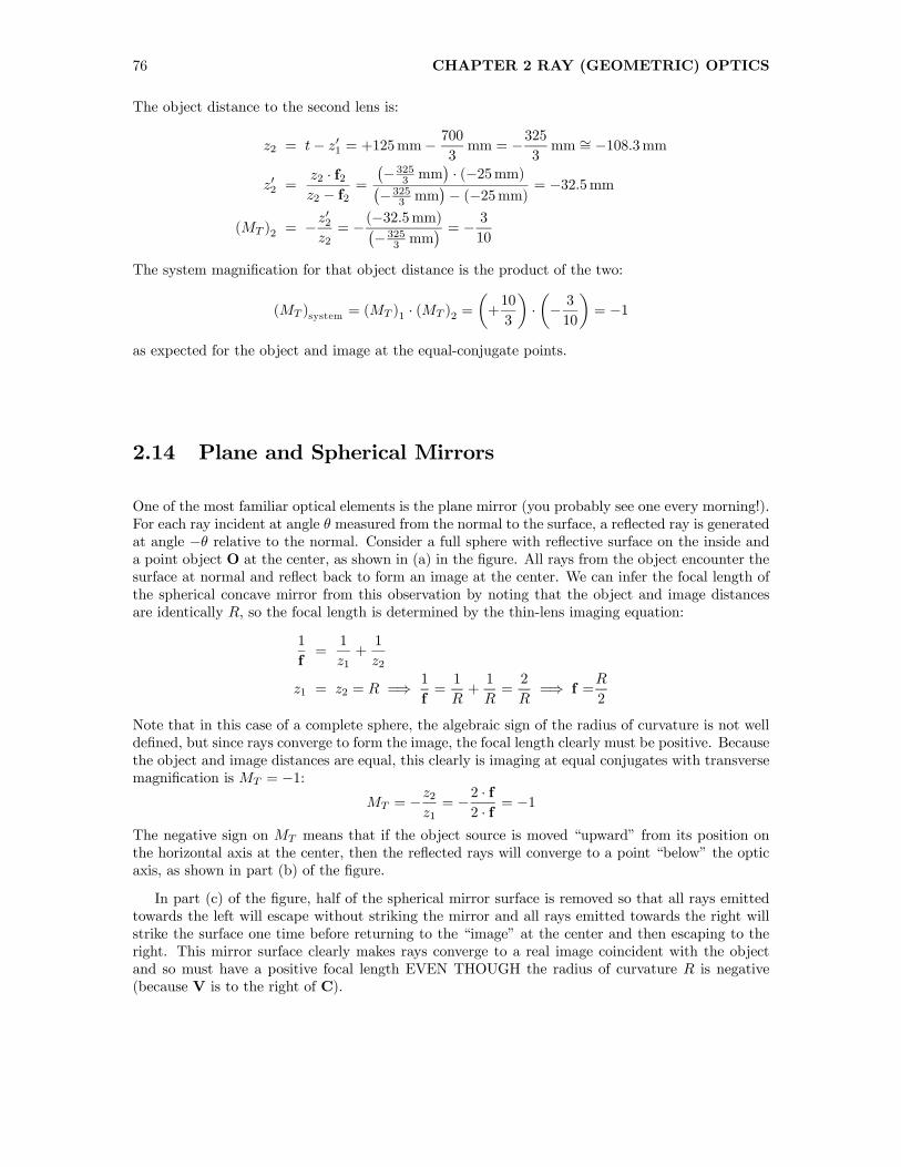
76 CHAPTER 2 RAY (GEOMETRIC) OPTICS
The object distance to the second lens is:
z2 = t− z01 = +125mm−700
3mm = −325
3mm ∼= −108.3mm
z02 =z2 · f2z2 − f2
=
¡−3253 mm
¢· (−25mm)¡
−3253 mm¢− (−25mm)
= −32.5mm
(MT )2 = −z02z2= −(−32.5mm)¡
−3253 mm¢ = − 3
10
The system magnification for that object distance is the product of the two:
(MT )system = (MT )1 · (MT )2 =
µ+10
3
¶·µ− 310
¶= −1
as expected for the object and image at the equal-conjugate points.
2.14 Plane and Spherical Mirrors
One of the most familiar optical elements is the plane mirror (you probably see one every morning!).For each ray incident at angle θ measured from the normal to the surface, a reflected ray is generatedat angle −θ relative to the normal. Consider a full sphere with reflective surface on the inside anda point object O at the center, as shown in (a) in the figure. All rays from the object encounter thesurface at normal and reflect back to form an image at the center. We can infer the focal length ofthe spherical concave mirror from this observation by noting that the object and image distancesare identically R, so the focal length is determined by the thin-lens imaging equation:
1
f=
1
z1+1
z2
z1 = z2 = R =⇒ 1
f=1
R+1
R=2
R=⇒ f =
R
2
Note that in this case of a complete sphere, the algebraic sign of the radius of curvature is not welldefined, but since rays converge to form the image, the focal length clearly must be positive. Becausethe object and image distances are equal, this clearly is imaging at equal conjugates with transversemagnification is MT = −1:
MT = −z2z1= −2 · f
2 · f = −1
The negative sign on MT means that if the object source is moved “upward” from its position onthe horizontal axis at the center, then the reflected rays will converge to a point “below” the opticaxis, as shown in part (b) of the figure.
In part (c) of the figure, half of the spherical mirror surface is removed so that all rays emittedtowards the left will escape without striking the mirror and all rays emitted towards the right willstrike the surface one time before returning to the “image” at the center and then escaping to theright. This mirror surface clearly makes rays converge to a real image coincident with the objectand so must have a positive focal length EVEN THOUGH the radius of curvature R is negative(because V is to the right of C).

2.14 PLANE AND SPHERICAL MIRRORS 77
Spherical mirror: (a) rays from point source at center of sphere are all normal to the surface andreflect back upon themselves to form a point image at object, so that z1 = z2 = R; (b) if the pointsource is moved “upward”, the image moves “downward,” which shows that MT = −1; (c) half the
sphere is removed leaving a hemisphere with R = CV < 0.
Derivation of the focal length of a concave spherical mirror. The magnified section at the bottomshows the triangles used to evaluate f in terms of R: f =R
2 in the paraxial approximation.
We can consider the hemispherical concave mirror with radius of curvature R = VC < 0. Eventhough the radius is negative, we have already inferred that the focal length of this system is positivesince the image rays converge, so we have:
f =|R|2=−R2= −R
2

78 CHAPTER 2 RAY (GEOMETRIC) OPTICS
A ray from an object at infinity that is close to (and parallel to) the optical axis, as shown in the inthe figure. From triangle ∆CAV in the magnified view, it is apparent that:
sin [θ] =x
CV=
x
−VC=
x
−RFrom ∆F0AV, we see that
tan [2θ] =x
F0V0
Now apply the paraxial approximation that sin [θ] ∼= tan [θ] ∼= θ if θ ∼= 0:
sin [θ] =x
−R∼= θ =⇒ x = −R · θ
tan [2θ] =x
f∼= 2θ =⇒ x = f · 2θ
Now equate the two terms to find a relationship between f and R:
−R · θ = f · 2θ =⇒ f = −R2
This expression for the focal length may be substituted into the imaging equation for a single thinlens:
1
z1+1
z2=1
f= − 2
R
For the case just considered of a concave surface, R < 0 and f > 0. If the object distance z1 > f ,then the image distance z2 is positive, BUT IS MEASURED FROM RIGHT TO LEFT. If themirror is a convex spherical surface with R = VC > 0; the image of a ray from an object at infinitycrosses the axis at the image-space focal point behind the mirror, so the optic makes rays divergeand therefore has negative power.
Convex mirror has positive radius of curvature (R > 0) but the reflected rays diverge and so the
surface has negative focal length via f = −R2.

2.15 STOPS AND PUPILS 79
2.14.1 Comparison of Thin Lens and Concave Mirror
Comparison of the vertices, focal points, principal points, and equal-conjugate points of a concavemirror and a thin lens. The vertices and the principal points coincide in both cases so that
MT = +1 for object and image at the vertex of the mirror and at the surfaces of the lens. Theobject- and image-space focal points of the mirror coincide at the distance feff = −R
2 for the mirror,and the equal conjugate points are located at the center of curvature so that z1 = z2 = 2feff . For the
lens, the equal conjugate points are also located such that z1 = z2 = 2feff with MT = −1.
2.15 Stops and Pupils
In any multielement optical system, the beam of light that passes through the system is shaped likea solid circular “spindle” with different radii at different axial locations. A larger exiting ray conemeans that more light reaches the image to make it brighter, so the diameter of this specific elementis the limiting factor for image “brightness.” The diameter of one optical element will limit the sizeof the ray spindle that exits the system; this limiting element is the aperture stop of the system andmay be a lens or an aperture with no power (an iris diaphragm) that is placed specifically to limitthe diameter of the ray cone. Consider the example of a two-lens system with an iris positionedbetween them shown in the figure. The iris limits the cone of rays from the object at O

80 CHAPTER 2 RAY (GEOMETRIC) OPTICS
Schematic of the aperture stop S and entrance and exit pupils E and E0, respectively for a systemformed from two positive lenses and an iris with no power. The entrance pupil E is the image ofthe stop S seen from the left through the first lens L1, while the exit pupil is the image of S seenfrom the right through the second lens L3. Note that the element that is the stop may vary with
object location O.
Obviously, the aperture stop in an imaging system composed of a single lens is that lens. In atwo-element system, the stop will be one of the two lenses, determined by the relative diametersand the locations of the lenses. The image of the stop seen from the input “side” of the lens is theentrance pupil, which determines the angular spread of the ray cone from an object point that “getsinto” the optical system, and thus determines the “brightness” of the image. The image of the stopseen from the output “side” is the exit pupil (once called the Ramsden disk).In an imaging system intended for viewing by eye, it is useful to locate the exit pupil at the iris
of the eye and to match its diameter to that of the iris of the eye to ensure that all light throughthe optical system makes it into the eye to form the viewable image.
2.15.1 Focal Ratio — f-number
For multilens systems, the size of the entrance pupil determines the angular extent of the ray conethat enters the system from a point source. The figure shows a simple hypothetical imaging systemwith object-space and image-space principal points H and H0, respectively and aperture stop ofdiameter d0 as the first element in the system (the same analysis applies for systems with theentrance pupil at other locations for an object at infinity). In this system, the stop is also is theentrance pupil. A point source at infinity creates a plane wave through the entrance pupil, which isthen incident on the object-space principal plane H with the same diameter. The unit transversemagnification of the two principal planes ensures that the light emerging from the image-space

2.15 STOPS AND PUPILS 81
principal plane H0 has that same diameter d0 = dNP. The cone angle of rays incident on the imageplane at the image-space focal point F0 is the ratio of the diameter to the distance H0F0 = feff :
d0feff
=dNPfeff
This means that the focal ratio of the system is:
f/# =feffdNP
Note that a corresponding expression could be constructed based on the diameter of the exit pupil,but the propagation distance then would have to be the distance from the exit pupil to the image,which (in this case) is longer than the effective focal length.
Specification of the system focal ratio: the plane wave from a point source at infinity is incidentthrough the aperture stop with diameter d0 onto the object-space principal plane H. The light
emerging from the image-space principal plane H0 has the same diameter d0. The light propagatesthe focal length feff to the image. The angle of the ray cone is d0
feff,which is the system focal ratio
f/#.
This f-number specifies the ability of the system to collect light.
2.15.2 Example: Focal Ratio of Lens-Aperture Systems
The focal ratio of a single thin lens obviously is the ratio of the focal length to the diameter of thelens:
f/# =f
d0
Note that the smallest possible focal ratio exists for a full sphere (which is anything but thin andthe paraxial approximation certainly does not apply over its full diameter). It might be useful todetermine the focal ratio for such a case with “normal” glass (n = 1.5). The focal length of the

82 CHAPTER 2 RAY (GEOMETRIC) OPTICS
sphere in the (ridiculously invalid) thin-lens paraxial approximation where R = 12.5mm is obtainedfrom the lensmaker’s equation:
f =
µ(n2 − 1)
µ1
R1− 1
R2
¶¶−1= (1.5− 1)
µ1
12.5mm− 1
−12.5mm
¶−1= 3.125mm
The focal ratio is:
f/# =f
d0=3.125mm
25mm=1
8
This is ridiculously invalid because it assumes that the sphere is simultaneously “thin” and “fat”If we assume the spherical lens is composed of two thin lenses at the vertices with the power of
a single surface:
f1 = f2 =
µ1.5− 112.5mm
¶−1= 25mm
t = 25mm
feff =f1 · f2
f1 + f2 − t=
25mm · 25mm25mm+ 25mm− 25mm = 25mm
BFL =(f1 − t) · f2f1 + f2 − t
= 0
Single Thin Lens + Aperture “in front”
Consider a system with a diaphragm (iris or aperture) of diameter d0 located at a distance t “infront” of the lens with focal length f1 and diameter d1. Since the aperture has no power to refractlight (φ = 0 diopters), then its “focal length” is infinite (f0 =∞). The focal length of the two-“lens”system is:
feff =f0 · f1
(f0 + f1)− t= f1 · lim
f0→∞
µf0
(f0 + f1)− t
¶= f1
which makes sense: the focal length of a system consisting of one refracting element and one “non-refracting” element is that of the refracting lens.For an object at infinity (z1 =∞ =⇒ z2 = f1), the diaphragm is the aperture stop if its diameter
is smaller than that of the lens:
d0 < d1 =⇒ iris is aperture stop
and the iris is also the entrance pupil. The focal ratio of the system is:
f/# =f1d0
The exit pupil may be located by applying the imaging equation:
zXP =t · f1t− f1
which shows that the exit pupil is virtual (“behind” the lens as seen from image space) if t < f1.Note that if t = f1 so that the aperture is located at the object-space focal point of the system, thenthe distance from the lens to the exit pupil is infinite: the system is “telecentric in image space.”The exit pupil is real (and may be visualized on an observation screen) if zXP > 0 =⇒ t > f1.Consider some examples with f1 = 100mm, d1 = 25mm, t = 25mm, and d0 = 10mm. If the iris

2.15 STOPS AND PUPILS 83
is deleted, then the focal ratio is:
f/# =feffd1=100mm
25mm= f/4
The iris is the stop and entrance pupil. The location of the exit pupil is:
zXP =t · f1t− f1
=25mm · 100mm25mm− 100mm = −100
3mm
MXP = −−1003 mm
25mm= +
4
3
dXP = d0 ·MXP =40
3mm = 13
1
3mm
The iris is the stop and entrance pupil, so the focal ratio is:
f/# =feffdNP
=100mm
10mm= f/10
Single Thin Lens + Aperture “behind”
If the lens comes first in the system, then we need to find the condition of the iris diameter todetermine if it is the aperture stop. At some risk of confusion, we’ll maintain the notation where thediameter of the lens is d1 and that of the aperture is d0 even though it is second in the system. Foran object at infinity, the figure shows that the distance to the iris must be less than the focal lengthto have any possibility of being the aperture stop. The image of the aperture seen from object spaceis located at
z =t · f1t− f1
which is positive (so the entrance pupil is real) if t < f1. The transverse magnification of the entrancepupil is:
MT =z
t=
f1t− f1
which implies that the diameter of the image of the iris is:
d00 =MT · d0
If we use the same numerical values as before but with the iris “behind,” the distance to the entrancepupil is:
zNP =t · f1t− f1
=25mm · 100mm25mm− 100mm = −100
3mm
MNP = −zNP
25mm= −−1003 mm
25mm= +
4
3
dNP = +4
3· 10mm = 40
3mm
This is the diameter of the incoming beam at the lens, so the focal ratio is:
f/# =feffdNP
=100mm403 mm
= f/7.5

84 CHAPTER 2 RAY (GEOMETRIC) OPTICS
Three examples of systems: the first is a single thin lens with the aperture stop at the lens, so thestop coincides with the entrance and exit pupils; the second moves the iris “in front” of the lens sothat it is also the entrance pupil; in the third, the iris is behind the lens and the magnified diameter
of the entrance pupil is the relevant parameter for the focal ratio.

2.15 STOPS AND PUPILS 85
2.15.3 Example: Exit Pupils of Telescopic Systems
Galilean Telescope
In the example of a telescopic system, such as binoculars, composed of an objective lens L1 withdiameter d1 and an eyelens L2 with diameter d2, where the two lenses are separated by the sumof their focal lengths. Consider the specific example of a Galilean telescope with f1 = +200mm,D1 = 50mm, f2 = −25mm, D2 = 25mm, and t = f1+ f2 = 175mm. We have already seen that theangular magnification of the system is the ratio of the focal lengths of the two lenses:
Mθ = −f1f2= −+200mm−25mm = +8
To determine which element is the aperture stop for a ray incident from an object at infinity, weneed to determine where this ray strikes the second lens. In this case, it strikes well within the lensdiameter — the ray height from the first lens is:
y =d12·µ1− t
f1
¶= 25mm ·
µ1− 175mm
200mm
¶=25
8mm = 3.125mm <
d22
so the first lens is the aperture stop, and therefore also the entrance pupil.
Location of aperture stop for the specified Galilean telescope. Since the ray from infinity that strikesthe edge of the positive lens passes well within the boundary of the negative lens, the aperture stop
is the positive lens for an object at infinity.
The exit pupil is the image of the aperture stop (first lens) seen through the second lens, whichhas negative focal length, ensuring that the exit pupil will be virtual. The distance from the stopto the second lens is:
z2 = t = f1 + f2 = 175mm
and the image distance from the second lens is:
z02 =z2 · f2z2 − f2
=175mm · (−25mm)175mm− (−25mm) = −
175
8mm = −21.875mm

86 CHAPTER 2 RAY (GEOMETRIC) OPTICS
Figure 2.1:
The size of the exit pupil is determined from the transverse magnification:
MT = −z02z2= −− 1758 mm
175mm= +
1
8
Since the diameter of the stop is d1 = 50mm, the diameter of the exit pupil is:
dXP =MT · dStop = +1
8· 50mm = +6.25mm
For the Galilean telescope, the exit pupil is virtual (located 21.875mm “behind” the eyelens) andsmall.
Keplerian Telescope
Now repeat the analysis for a corresponding Keplerian telescope with f1 = +200mm, d1 = 50mm,f2 = +25mm, d2 = 25mm, t = f1 + f2 = 225mm and angular magnification:
Mθ = −f1f2= −+200mm
+25mm= −8
Again, the height of the ray at the edge of the first lens from an object at infinity has height atthe second lens:
y =d12·µ1− t
f1
¶= 25mm ·
µ1− 225mm
200mm
¶= −25
8mm = −3.125mm
|y| < d22
The first element is still the stop and the entrance pupil. The image of the first lens through the

2.15 STOPS AND PUPILS 87
second is the exit pupil; its location and size are determined using the thin-lens imaging equation:
z2 = t = f1 + f2 = 225mm
z02 =z2 · f2z2 − f2
=225mm · 25mm225mm− 25mm =
225
8mm = +28.125mm
MT = −z02
z2= −
2258 mm
225mm= −1
8
dXP = dStop ·MT = 50mm ·µ−18
¶= −6.25mm
The exit pupil is “real” (outside of the system at a distance of 28.125mm beyond the eyelens) andinverted.
In both of the telescopes just considered, note that the diameter of the exit pupil is the ratio ofthe focal length of the eyepiece and the focal ratio of the object lens:
dXP =f2³f1d1
´ = d1³f1f2
´ = d1Mθ
(dXP)Galilean =50mm
+8= 6.25mm
(dXP)Keplerian =50mm
−8 = −6.25mm
In words, the diameter of the exit pupil is equal to the ratio of the diameter of the entrance pupil(which is the objective in this case) and the magnifying power; more power means a smaller exitpupil.
Common binoculars used for birdwatching are listed as “10× 50,” which means that the angularmagnification (magnifying power) is 10 and the diameter of the entrance pupil (which is that of theobjective lens0 is 50mm / 2 in. The diameter of the eyelens is:
dXP =50mm
10= 5mm
Until recently, the most common variety of binocular was the “7 × 50,” which has a magnifyingpower of 7 and objectives with d = 50mm, so the diameter of the exit pupil is:
dXP =50mm
7' 7mm
This is a close match to the diameter of the iris of the dark-adapted eye and thus are a good choicefor astronomical viewing; for that reason, 7 × 50 binoculars were known as “night glasses.” Whenused with the smaller iris diameter of the eye during daytime, much of the diameter of the exit pupilwould illuminate the opaque iris and not contribute to the brightness of the image on the retina.
For a formerly common amateur telescope with a mirror objective with d1 = 6 in ∼= 150mm anda focal length f1 = 48 in ∼= 1220mm, the focal ratio is:
f/# =48 in
6 in= 8
so the diameter of the exit pupil is when viewed through an eyelens with focal length f2 is
dXP =f2
f/#=f28
If the focal length of the eyelens is f2 = 25mm ∼= 1 in, then the diameter of the exit pupil is about3mm, which is pretty small. If the focal length of the eyelens is f2 = 4mm ∼= 1
6 in, the magnifying

88 CHAPTER 2 RAY (GEOMETRIC) OPTICS
power of the system is:
Mθ =f1f2∼=48 in16 in
= +288
which is a large number that will impress a naive user. BUT the diameter of the exit pupil is verysmall
dXP =f28=
16 in
8=1
48in ∼= 0.5mm
so it would be very difficult to “see” anything through this telescope. This illustrates the flaw in thestrategy that was once used often by manufacturers of cheap telescopes intended as gifts for children;the manufacturers would often quote a very large value for the magnifying power that required aneyepiece with a very short focal length and therefore a very small exit pupil. The images were verydifficult to see by novices and experienced users alike.
The location of the exit pupil also is important. It is useful to have it placed “outside” theimaging system where the eye would be located so that it is feasible to get all of the light throughthe pupil into the eye. The distance from the rear vertex of the system to the exit pupil is the eyerelief :
V0E0 = eye relief
An imaging system with “lots of” eye relief may be easier to view through, since the location wherethe eye is optimally placed is back away from the eyelens. An example of a system that needs alarge eye relief is a rifle scope, where the eyepiece lens will be located “far” in front of the viewingeye.
For different object distances, it is possible for the aperture stop to “move around,” i.e., theelement that defines the aperture stop may change with object distance. The locations and sizes ofthe pupils are determined by applying the ray-optics imaging equation to these objects. To some,the concept of finding the “image of a lens” may seem confusing, but it is no different from before— just think of the lens as a regular opaque object at its location and find the images through theoptics that come after (for the exit pupil) or that came before (entrance pupil).
Which element in a multielement system is the “stop” depends on the relative sizes of the lenses.In the first case shown below, the first lens (the objective) is small enough that it acts as the stop(and thus also the entrance pupil). The image of the objective lens seen through the eyelens is theexit pupil, and is “between” the two lenses and very small. Because the exit pupil is small and“remote” (located “within” the optical system), so is the field of view of the Galilean telescope. Inthe second example, the smaller eyelens is the stop and also the exit pupil, while the image of theeyelens seen through the objective is the entrance pupil and is far behind the eyelens and relativelylarge.
More Examples of Galilean and Keplerian Telescopes
Consider the two two-lens telescope designs. The Galilean telescope has a positive-power objectiveand a negative-power ocular or eyelens. The Keplerian telescope has a positive objective and apositive eyelens. Assume that the objective is identical in the two cases with f1 = +100mm andd1 = 30mm. The focal lengths and diameters of the oculars (eyepieces) are f = ±15mm andd2 = +15mm (these are the approximate dimensions and focal lengths of the lenses in the OSAOptics Discovery Kit). The lenses of a telescope are separated by f1 + f2, (f1 + f2 ∼= 85mm and115mm for the Galilean telescope and Keplerian telescope, respectively). We want to locate thestops and pupils. The stop is found by tracing a ray from an object at ∞ through the edge of thefirst element and finding the ray height at the second lens. If this ray height is small enough to passthrough the second lens, then the first lens is the stop; if not, then the second lens is the stop.

2.15 STOPS AND PUPILS 89
Galilean telescope for object at z1 = +∞: (a) the objective lens is the aperture stop and entrancepupil because it limits the cone of entering rays. The image of the stop seen through the eyelens isthe (very small) exit pupil; (b) the larger objective means that the eyelens is the aperture stop andthe exit pupil. The image of the eyelens seen through the objective is the entrance pupil, and isbehind the eyelens because the object distance to the objective is less than the focal length.
Consider the Galilean telescope first. The ray height at the first lens is the “semidiameter” of thelens: d1
2 = 15mm; it is not called the “radius” to avoid confusion with a “radius of curvature.” Fromthere, the ray height would decrease to 0mm at a distance of f1 = +100mm, but it first encountersthe negative lens at a distance of t = +85mm. The ray height at this lens is
100mm− 85mm100mm
· 15mm = 2.25mm
which is much smaller than the lens semidiameter of d22 = 7.5mm. Hence the first lens (the objectivelens) is the stop.The entrance pupil is the image of the stop through all of the elements that come before the stop.
In this case, the first lens is also the entrance pupil and its transverse magnification is unity. Theexit pupil is the image of the stop through all elements that come afterwards, which is the negativelens. The distance to the “object” is f1 + f2 = 85mm, so the imaging equation is used to locate theexit pupil and determine its magnification:
1
85mm+1
z0=1
f2=
1
−15mm
z0 =
µ− 1
15mm− 1
85mm
¶−1= −51
4mm = −12.75mm
MT = −z0
z= −−12.75mm
85mm= 0.15
The exit pupil is upright, but more important, its distance from the second lens is negative; the exitpupil is a virtual image and not accessible to the eye. The viewer “sees” the exit pupil in front of

90 CHAPTER 2 RAY (GEOMETRIC) OPTICS
the eye. This limits the field of view of the Galilean telescope.Follow the same procedure to determine the stop and locate the pupils and their magnifications
for the Keplerian telescope. The ray height at the first lens for an object located at ∞ is again15mm. The ray height decreases to 0mm at the focal point, but then decreases still farther untilencountering the ocular lens at a distance of f1 + f2 = 115mm. The ray height h at this lens isdetermined from similar triangles:
15mm
−h =100mm
15mm=⇒ h = −2.25mm
So the first lens is the stop and entrance pupil (with unit magnification) in this case too. Thedistance from the stop to the second lens is f1 + f2 = 115mm, so the imaging equation for locatingthe exit pupil and determining its magnification is:
1
115mm+1
z0=1
f2=
1
+15mm
z0 =
µ+
1
15mm− 1
115mm
¶−1= +
69
4mm = +17.25mm
MT = −z0
z= −+17.25mm
85mm∼= −0.203
The exit pupil is a real image of the aperture stop in the Keplerian telescope — we can place our eyeat it and see a larger field of view.
Vignetting
The location of the aperture stop is determined for an object located “on” the optical axis. If theobject is “off” the axis, the cone of rays that get throught the system is “skewed” or “tilted.” Ifother elements in the system (lenses or diaphragms) constrain parts of the skewed cone of rays,then the cone of rays is truncated and the brightness of the image is reduced; this phenomenon is“vignetting.”
Example of vignetting; the brightness of the scene at the edges is reduced due to the presence of an“out-of-focus” aperture in the system.
2.15.4 Pupils and Diffraction
The concept of pupils may be combined with diffraction to evaluate the effective focal ratio (f/number)of the imaging system. For a single thin lens, the diffraction spot is determined by the size and shapespecified by the pupil function p [x, y] or p (r) and the distance to the image. If the lens has a circular

2.16 MARGINAL AND CHIEF RAYS 91
pupil of diameter d0, the pupil function
p (r) = CY L
µr
d0
¶determines the extent of the ray cone that enters the system. We derived the resulting diffractionpattern, which is proportional to a scaled circularly symmetric sombrero function, which is theanalogue of the SINC function using the first-order Bessel function, and therefore is sometimescalled the “besinc” function.
h (r) ∝ πd204· SOMB
⎛⎝ r³λ0z2d0
´⎞⎠
If the object distance is large, then the image distance z2 ' f and the amplitude of the impulseresponse is:
h (r) ∝ SOMB
⎛⎝ r³λ0fd0
´⎞⎠
The diameter of the Airy disk is approximately:
D0∼= 2.44λ0
µf
d0
¶∼= 2.44 · λ0 · f/#
2.15.5 Field Stop
As suggested by its name, a field stop limits the field of view of the system. It may be as simple asthe finite size of the sensor (e.g., a rectangular piece of photosensitive emulsion or a CCD sensor),or it may be placed at an intermediate image within the system or even at the object itself. Imagesof the field stop are located at the same locations as intermediate images of the object.
2.16 Marginal and Chief Rays
Many important characteristics of an optical system, including the possible presence of vignetting,are determined by the trace of two specific rays through the imaging system. For an object O withimage O0, aperture stop S and entrance pupil E and exit pupil E0, the marginal ray traces from thecenter of O to the edge of S and back to the center of O0. The chief ray (or principal ray) is tracedfrom the edge of O (or edge of the “field of view”) hrough the center of S to the edge of O0. Since Eand E0 are images of the stop S, the marginal and chief rays also go through the edges and centersof the pupils, respectively.The marginal ray is specified by its ray heights y and ray angle u at different points on the
optical axis; the corresponding notation for the chief ray includes “overscores” or “bars:” y, u.Heights and angles of the marginal ray after refraction at a surface are “primed,” e,g, y0 and u0.The corresponding quantities for the chief ray are y0, and u0.From the definition of the marginal ray, an object or image is located at any location (value of
z) where y = 0. Similarly, the aperture stop, entrance pupil, and exit pupil are located at valuesof z where y = 0. An image exists wherever the marginal ray crosses the axis and the aperturestop or pupils are located wherever the chief ray crosses the axis. Complete specification of thesetwo rays is sufficient to characterize the location of object and image(s), the field of view, and themagnifications.The chief ray is the axis of the unvignetted light beam from a point at the edge of the field of view.
The radius of the unvignetted light beam (or perhaps more appropriately called the semidiameterto avoid potential confusion with the “radius of curvature) is the sum of the heights of the marginaland chief rays:
dunvignetted2
= y + y at any location z

92 CHAPTER 2 RAY (GEOMETRIC) OPTICS
Figure 2.2: The marginal and chief rays for a two-element imaging system where the second elementis the stop. The marginal ray comes from the center of the object O, grazes the edge of the stop andthrough the center of the image O0. The chief ray travels fromt the edge of the object through thecenter of the stop to the edge of the image.
Because paraxial calculations are linear, it is customary to normalize the ray heights and anglesfor the calculation and then scaling the results to satisfy the conditions of the specific system. Forexample, we generally select the chief ray height y = 1 and the marginal ray angle u = 1 at the object.Clearly the choice of unit ray angle (in radians) is inconsistent with the paraxial approximation, butthis is just a computational convenience because all quantities are scalable.
2.16.1 Telecentricity
If the aperture stop is located such that the entrance and/or exit pupils are at infinity, then thesystem is telecentric. One way to do this is to place the aperture stop at one of the focal points ofthe system, which means that the corresponding pupil is at the same location and the other pupilis at infinite. As shown in the figure, if the stop is located at the object-space focal point of a singlethin lens, then the entrance pupil is at the same location and the exit pupil is at infinity in imagespace — this is an image-space telecentric system.

2.16 MARGINAL AND CHIEF RAYS 93
Telecentric system consisting of single thin lens with aperture stop placed at object-space focal point,showing chief ray (solid blue) and marginal ray (red). The chief intersects the optical axis at thatfocal point and so emerges from the lens parallel to the optical axis. The dashed blue lines parallel tothe chief ray intersect at the image. The defocused image is the same height as the focused image.
If the stop is located at the image-space focal plane, then the entrance pupil is at infinity, formingan object-space telecentric system. If either the entrance or exit pupil is at infinity, then the chiefray must be parallel to the optical axis on that side of the imaging system. This means that thesystem transverse magnification will be constant even if the image is blurry. Put another way, ablurred image has the correct magnification.A “double telecentric” system is an afocal system (telescope) with the stop located at the common
focal plane of the two lenses. This means that both the entrance and exit pupils are at infinity. Thefact that the magnification of the system does not depend on accuracy of focusing makes telecentricsystems particularly useful for metrology.
Double telecentric system with the aperture stop at the common focal point of the two lenses. Themarginal ray is shown in red and the chief ray in solid blue.

94 CHAPTER 2 RAY (GEOMETRIC) OPTICS
2.16.2 Marginal and Chief Rays for Telescopes
The marginal ray of an afocal system used to image an object at infinity travels parallel to theoptical axis before the first lens and after the last (u = 0, u0 = 0). The relative sizes of the twolenses determine which is the aperture stop — for a Galilean telescope, the aperture stop is usuallythe negative ocularlensMORE TO COME

Chapter 3
Tracing Rays Through OpticalSystems
The imaging equation(s) become quite complicated in systems with more than a very few lenses.However, we can determine the effect of the optical system by ray tracing, where the action ontwo (or more) rays is determined. Raytracing may be paraxial or exact. Historically, graphical,matrix, or worksheet ray tracing were commonly used in optical design, but most ray tracing is nowimplemented in computer software so that exact solutions are more commonly implemented thanheretofore.
3.1 Paraxial Ray Tracing EquationsConsider the schematic of a two-element optical system made of thick lenses, so the vertices andprincipal planes of individual lenses do not coincide at the same points.
Schematic of ray tracing of a provisional marginal ray from an object at an infinite distance. Thesystem has two elements and the locations Hn and H 0
n are the principal planes of the nth element.The ray height at the nth element is yn and the ray angle during transfer between elements n− 1
and n is un.
The two elements are represented by their two principal “planes”, which are the planes of unitmagnification. The refractive power of the first element changes the ray angle of the input ray. Inthe example shown, the input ray angle u1 = 0 radians, i.e., the ray is parallel to the optical axis.The height of this ray above the axis at the object-space principal plane H1 is y1 units. The ray
95

96 CHAPTER 3 TRACING RAYS THROUGH OPTICAL SYSTEMS
Figure 3.1: Refraction of a paraxial ray at a surface with radius of curvature R between media withrefractive indices n and n0. The ray height and angle at the surface are y and u, respectively. Theangle of the ray measured at the center of curvature is α. The height and angle immediately afterrefraction are y and u0. The object and image distances are s and s0 (which are now called z andz0 in the text).
emerges from the principal plane H01 at the same height y1 but with a new ray angle u2. The ray
“transfers” to the second element through the distance t2 in the index n2 and has ray height y2 atprincipal plane H2. The ray emerges from the principal plane at the same height but a new angleu3.
3.1.1 Paraxial Refraction
Consider refraction of a paraxial ray emitted from the object O at a surface with radius of curvatureR. For a paraxial ray, the surface may be drawn as “vertical”. The height of the ray at the surfaceis y.
From the drawing, the incoming ray angle u measured from the optical axis is:
u = tan−1hyz
i∼=
y
z> 0
and the corresponding equation for the outgoing ray measured from the optical axis is:
u0 = tan−1h yz0
i∼=
y
z0> 0
The angle of the height of the ray at the refractive surface measured from the center of curvature is:
α = − tan−1h yR
i∼= −
y
R
The incident and refracted angles measured from the surface at height y are the angles of incidenceand refraction. From the drawing:
i = u− α
i0 = u0 − α

3.1 PARAXIAL RAY TRACING EQUATIONS 97
Now apply Snell’s law in the paraxial approximation:
n sin [i] = n0 sin [i0] =⇒ n · i ∼= n0 · i0
n · (u− α) = n0 · (u0 − α)
=⇒ n0u0 ∼= nu− nα+ n0α = nu+ α (n0 − n)
= nu+³− y
R
´· (n0 − n)
= nu− y · (n0 − n)
R≡ nu− y · φ
n0u0 ∼= nu− y · φ
The paraxial refraction equation in terms of the incident angle u, refracted angle u0, ray height y,
surface power φ =1
f, and indices of refraction n and n0 is:
φ =n0u0 − nu
y
3.1.2 Paraxial Transfer
Paraxial transfer from one surface to the next in a medium with refractive index n0.
The transfer equation determines the ray height y0 at the next surface given the initial ray heighty, the physical distance t0 and the ray angle u0 in the medium with index n0. From the drawing, wehave:
y0 = y + t0 · u0
y0 = y +
µt0
n0
¶· (n0u0)
where the substitution was made to put the ray angle in the same form n0u0 that appeared in therefraction equation. The distance t0
n0 ≤ t0 is called the reduced thickness (note the potential for

98 CHAPTER 3 TRACING RAYS THROUGH OPTICAL SYSTEMS
confusing reduced thickness t0
n0 and optical path length n0t0).
3.1.3 Linearity of the Paraxial Refraction and Transfer Equations
Note that both the paraxial refraction and transfer equations are linear in the height and angle,i.e., neither includes any operations involving squares or nonlinear functions (such as sine, tangent,or logarithm). Among other things, this means that they may be scaled by direct multiplicationto obtain other “equivalent” rays, as to match the marginal ray height to the semidiameter of theaperture stop or the chief ray angle to the semidiameter of the field stop. For example, the outputangle may be scaled by scaling the input ray angle and the height by a constant factor α:
α (nu− yφ) = α · (nu)− (α · y)φ = α (n0u0)
We will take often advantage of this linear scaling property to scale rays to to find the exact marginaland chief rays from the provisional counterparts.
3.1.4 Paraxial Ray Tracing
To characterize the paraxial properties of a system, two provisional rays are traced:
1. Initial height of marginal ray at first surface: y = 1.0, initial marginal ray angle nu = 0;
2. Initial height of chief ray at first surface: y = 0.0, initial chief ray angle nu = 1.
We have already named these rays; the first is the provisional marginal ray that intersects theoptical axis at the object (and thus also at every image of the object). The second ray (distinguishedby the overscore) is called the provisional chief (or principal) ray and travels from the edge of theobject to the edge of the field of view through the center of the stop (and thus through the center ofthe pupils, which are images of the stop). Since the paraxial ray tracing equations are linear, theseprovisional rays may be scaled to the parameters of the system.
The process of ray tracing is perhaps best introduced by example. Consider a two-elementthree-surface system. The first surface is the cornea, with radius of curvature in the model ofR1 = +7.8mm. The “aqueous humor” between the cornea and the lens has a thickness of in themodel of 3.6mm and refractive index of n2 = 1.336. The surfaces of the lens have curvaturesR2 = +10mm, and R3 = −6mm, thickness of 3.6mm, and refractive index n3 = 1.413. The “vit-reous humor” between the lens and the retina has the same refractive index of n4 = 1.336 as the“aqueous humor.”

3.1 PARAXIAL RAY TRACING EQUATIONS 99
Marginal and chief rays traced through the three-surface optical system.
The refraction at the first surface changes the angle but not the height of a ray from the object.If the incident ray angle is 0 radians, then the new ray angle for the provisional marginal ray is:
(n0u0)1 = (nu)1 − y1 [mm] · φ1£mm−1
¤= 0− (1.0) (+0.043077)= −0.043077 radian
Note that we are retaining 6 decimal places in this calculation to ensure the best result at the end.We will then truncate (round) the value to a more reasonable accuracy.
The transfer equation for the provisional marginal ray between the first and second surfacechanges the height of the ray but not the angle. The height at the second surface is:
y01 = y1 +
µt0
n0
¶1
(n0u0)1 [mm]
= 1 +3.6
1.336(−0.043077) = +0.883924mm
Thus the ray exits the first surface at the “reduced angle” n0u0 ∼= −0.04 radians and arrives at thesecond surface at height y0 ∼= +0.88 units. The corresponding equations for the chief ray at the firstsurface are:
(n0u0)1 = (nu)1 − y1φ1= 1− (0.0) (+0.043077)= 1 radian

100 CHAPTER 3 TRACING RAYS THROUGH OPTICAL SYSTEMS
y01 = y1 +
µt0
n0
¶1
(n0u0)1
= 0 +3.6
1.336(1) = +2.694611mm ∼= 2.695mm
Since the provisional chief ray went through the center of the lens, its angle did not change. Theheight of the chief ray at the second surface is proportional to the ray angle.
Ray-Tracing Table
The equations may be evaluated in sequence to compute the rays through the system. These arepresented in the table. Each column in the table represents a surface in the system and the “primed”quantities refer to distances and angles following the surface. In words, t0 in the first row are thedistances from the surface in the column to the next surface.
Param ete r In it ia l S u r fa c e 1 S u r fa c e 2 S u r fa c e 3 Im ag e S u rfa c e
R +7.8mm +10.0mm −6.0mmt0 3.6mm 3.6mm
n0 1.0 1.336 1.413 1.336
−φ = −n0−nR
−0.043077mm−1 −0.007700mm−1 −0.012833mmt0n0
3.6mm1.336
= 2.694611mm 3.6mm1.413
= 2.54771mm 12.699 mm ⇓
R ay s ⇓
y 1mm 1mm 0.883924mm 0.756833mm 0mm
n0u0 0 −0.043077 r a d ia n −0.049883 r a d ia n −0.059596 r a d ia n −0.059596 r a d ia n
y 0mm 2.694611mm 5.189519mm 16.779317mm
n0u0 1 r a d ia n 1 r a d ia n 0.979251 r a d ia n 0.912654 r a d ia n
The raytrace indicates that the provisional marginal ray emerges from the last surface with height
and angle
⎡⎣ y
n0u0
⎤⎦ =⎡⎣ 0.756833mm
−0.059596 radians
⎤⎦. These are used to calculate the (boxed) distance tothe image location (where the marginal ray height is 0):
y0 = 0 = y +t0
n0(n0u0)
0 = (+0.756833) +t0
n0(−0.059596)
=⇒ t0
n0=+0.756833
0.059596∼= +12.699mm
This is the “reduced distance” in the image medium with index n4; the physical distance t0 is:
=⇒ t0 =+0.756833
0.059596mm · n0 = 12.699 · 1.336 ∼= 16.966mm
The height and angle of the provisional chief ray at the image location are y ∼= 16.78mm andn0u0 ∼= 0.91 radians, respectively, which may be scaled to the size of a known sensor to determinethe field of view.This particular system is often used as a model for the human eye with the lens “relaxed” to view
objects at ∞. The first surface represents the cornea of the eye, while the other two surfaces arethe front and back of the lens. Note that the power of the cornea (0.043077mm−1 ∼= 43 diopters) isconsiderably larger than the powers of the lens surfaces (7.7 diopters and 12.8 diopters, respectively).
3.2 Matrix Formulation of Paraxial Ray Tracing
The same linear paraxial ray tracing equations may be conveniently implemented as matrices actingon ray vectors for the marginal and chief rays whose components are the height and angle. The ray

3.2 MATRIX FORMULATION OF PARAXIAL RAY TRACING 101
vectors may be defined as:
paraxial marginal ray vector :
⎡⎣ y
nu
⎤⎦paraxial chief ray vector :
⎡⎣ y
nu
⎤⎦Note that there is nothing magical about the convention for the ordering of y and nu (i.e., which goes“on top” of the vector); this is the convention used by Roland Shack at the Optical Sciences Centerat the University of Arizona, but Willem Brouwer’s book “Matrix Methods in Optical InstrumentDesign” uses the opposite order. Note that the choice of convention here determines the form of thesystem matrix, but the two choices are equivalent.
In this notation, the two column vectors that represent the marginal and chief rays may becombined to form a ray matrix L:
L ≡
⎡⎣⎛⎝ y
nu
⎞⎠⎛⎝ y
nu
⎞⎠⎤⎦ =⎡⎣ y y
nu nu
⎤⎦which may be evaluated at any point in the system. The determinant of this ray matrix is:
det [L] = y · (nu)− (nu) · y ≡ ℵ
which we shall show to be a constant — the so-called Lagrange invariant. In words, the Lagrangeinvariant is the product of the chief ray height and marginal ray angle subtracted from the productof the marginal ray height and chief ray angle. We denote it by the symbol ℵ (“aleph,” chosen herefor the simple reason that it is distinctive). We shall see that ℵ is unaffected by both the refractionand transfer, and therefore is invariant as we progress through different locations in the system.
3.2.1 Refraction Matrix
Given the ray vectors or the ray matrix, we can now define operators for refraction and transfer.Recall that paraxial refraction of a marginal ray and of a chief ray at a surface with power φ changesthe ray angles but not the heights (at the surfaces):
n0u0 = nu− y · φ for marginal ray
n0u0 = nu− y · φ for chief ray
The refraction process for the marginal ray may be written as a matrix R and the output is theproduct with the ray vector which will have the same ray height and a different angle:
R
⎡⎣ y y
nu nu
⎤⎦ =
⎡⎣ y y
n0u0 n0u0
⎤⎦R =
⎡⎣ a c
b d
⎤⎦

102 CHAPTER 3 TRACING RAYS THROUGH OPTICAL SYSTEMS
where we need to evaluate the four values a− d. Consider the action of the refraction matrix on themarginal ray:
R
⎡⎣ y
nu
⎤⎦ =
⎡⎣ a c
b d
⎤⎦⎡⎣ y
nu
⎤⎦ =⎡⎣ y
n0u0
⎤⎦ay + c · (nu) = y =⇒ a = 1, c = 0
by + d · (nu) = n0u0 = nu− y · φ =⇒ b = −φ, d = 1
substitute these values to see the form of the refraction matrix:
R =
⎡⎣ 1 0
−φ 1
⎤⎦The determinant of the refraction matrix is:
detR = det
⎡⎣ 1 0
−φ 1
⎤⎦ = (1) (1)− (−φ) (0) = 1The action of a refraction matrix R on a ray matrix L is:
RL = L0⎡⎣ 1 0
−φ 1
⎤⎦⎡⎣ y y
nu nu
⎤⎦ =⎡⎣ y0 y0
n0u0 n0u0
⎤⎦=
⎡⎣ y y
nu− y · φ nu− y · φ
⎤⎦The determinant of the ray matrix after refraction is:
det£L0¤= y (nu− y · φ)− y (nu− y · φ)= y · nu− yy · φ− y · nu+ yy · φ= y · nu− y · nu = ℵ = det [L]
which confirms that the Lagrangian invariant is not affected by refraction.
3.2.2 Ray Transfer Matrix
The transfer of the marginal ray from one surface to the next within the medium with index n0 is
y0 = y +t0
n0(n0u0)
which also may be written as the product of a ray matrix T with the marginal ray vector:
T
⎡⎣ y
n0u0
⎤⎦ =⎡⎢⎣ y + (n0u0)
µt0
n0
¶n0u0
⎤⎥⎦=
⎡⎢⎣ 1µt0
n0
¶0 1
⎤⎥⎦⎡⎣ y
n0u0
⎤⎦ =⎡⎣ y0
n0u0
⎤⎦

3.2 MATRIX FORMULATION OF PARAXIAL RAY TRACING 103
so the determinant of the transfer matrix also is 1:
det
⎡⎢⎣ 1µt0
n0
¶0 1
⎤⎥⎦ = (1) (1)− (0)µ t0
n0
¶= 1
The action of the transfer matrix T on the ray matrix L is:
L0 = T L =
⎡⎣ y0 y0
n0u0 n0u0
⎤⎦ =⎡⎢⎣ 1
µt0
n0
¶0 1
⎤⎥⎦⎡⎣ y y
n0u0 n0u0
⎤⎦
=
⎡⎢⎣ y +
µt0
n0
¶· n0u0 y +
µt0
n0
¶· n0u0
n0u0 n0u0
⎤⎥⎦and the determinant of the ray matrix after the transfer operation is:
det [L0] = det [T L]
=
µy0 +
µt0
n0
¶n0u0
¶(n0u0)−
µy0 +
µt0
n0
¶nu
¶(n0u0)
= y0 · n0u0 +µt0
n0
¶n0u0 · n0u0 − y0 · nu−
µt0
n0
¶n0u0 · n0u0
= y0 · n0u0 − y0 · n0u0 = ℵ = det [L]
so the determinants of the ray matrix before and after refraction are also identically the Lagrangianinvariant ℵ; in other words, neither the refraction nor the transfer matrices has any effect on thedeterminant of a ray matrix, so the Lagrangian invariant is preserved by refraction or transfer (henceits name!).
Ray Transfer Matrix for an Optical System
The refraction and transfer matrices may be combined in sequence to model a complete system. Ifwe start with the marginal ray vector at the input object, the first operation is transfer to the firstsurface. The next is refraction by that surface, transfer to the next, and so forth until a final transferto the output image:
T nRn · · · T 2R2T 1R1T 0¡Lob ject
¢= Limage
If the initial ray matrix is located at the object (as usual), the marginal ray height is zero, so theray matrix at the object and any images has the form:
Lob ject =
⎡⎣ 0 yin
(nu)in (nu)in
⎤⎦Limage =
⎡⎣ 0 yout
(nu)out (nu)out
⎤⎦

104 CHAPTER 3 TRACING RAYS THROUGH OPTICAL SYSTEMS
so the system from object to image is:
S ≡ T nRn · · · T 2R2T 1R1T 0S · Lob ject = Limage
(T nRn · · · T 2R2T 1R1T 0)
⎡⎣ 0 yin
(nu)in (nu)in
⎤⎦ =⎡⎣ 0 yout
(nu)out (nu)out
⎤⎦Note that the individual refraction and transfer matrices are sequenced in inverse order, i.e., thelast matrix is the first in the sequence for the system. The transfer matrix T 0 acts on the input raymatrix, so it must appear on the right.
Ray Matrix for Provisional Marginal and Chief Rays
The system is characterized by using provisional marginal and chief rays located at the object. Thelinearity of the computations ensure that the rays may be scaled subsequently to satisfy other systemconstraints, such as the diameter of the stop. The provisional marginal ray at the object has heighty = 0 and ray angle nu = +1, while the provisional chief ray at the object has height y = +1 andangle nu = 0. Thus the provisional ray matrix at the object is:
L0 =
⎡⎣ 0 11 0
⎤⎦
3.2.3 “Vertex-to-Vertex Matrix” for System
We can construct a matrix that represents JUST the optical system by excluding the input raymatrix, the transfer matrix from object to object-space vertex, the transfer from image-space vertexto image, and the output ray matrix. This subset is the “vertex-to-vertex matrix” MVV0 of thesystem and is a complete specification of the paraxial properties of the system. The general formfor the matrix is:
MVV0=(Rn · · · T 2R2T 1R1) =
⎡⎣ A B
C D
⎤⎦where A,B,C,D are factors to be determined from the various refractions and transfers for a specificsystem. The entries A and D in the matrix are “pure” numbers (without units), while B and Dhave dimensions of length and reciprocal length, respectively. From matrix algebra, it is possible toshow that the determinant of the matrix product is the product of the determinants. We alreadyknow that the determinants of the matrices for any transfer or refraction is unity, which establishesa constraint on the vertex-to-vertex matrix:
det [MVV0 ] = detRn · detT n−1 · · · · · detR2 · detT 1 · detR1
= 1 · 1 · · · · · 1 · 1 = 1=⇒ det [MVV0 ] = 1
=⇒ AD −BC = 1
Consider a simple example of the matrixMVV0 for a two-lens system with powers φ1 = (f1)−1
and φ2 = (f2)−1 separated by t. The product of the two refraction matrices and the transfer matrix

3.2 MATRIX FORMULATION OF PARAXIAL RAY TRACING 105
is:
MVV0=R2T 1R1
=
⎡⎣ 1 0
−φ2 1
⎤⎦⎡⎣ 1 t
0 1
⎤⎦⎡⎣ 1 0
−φ1 1
⎤⎦=
⎡⎣ 1− φ1t t
− (φ1 + φ2 − φ1φ2t) 1− φ2t
⎤⎦MVV0=
⎡⎣ 1− φ1t t
−φeff 1− φ2t
⎤⎦where the known expression for the system power
1
feff=1
f1+1
f2− t
f1 · f2=⇒ φeff = φ1 + φ2 − φ1 · φ2 · t
has been substituted in the last expression. It is easy to confirm that the determinant of this systemmatrix is unity.We have four equations in the four unknowns A,B,C,D, which may be combined to find useful
systems metrics in terms of the elements in the vertex-to-vertex matrixMVV0 :
effective focal length of system feff =1
φeff= − 1
C
front focal length FFL =FV
n= −D
C
back focal length BFL =V0F0
n= −A
C
distance from front vertex to object-space principal pointVH
n=
D − 1C
distance from image-space principal point to rear vertexH0V0
n0=1−A
C
distance from rear vertex to image (if obj. dist. t1 is known)V0O0
n0=
t2n0=
m−A
C= −B −At1
D − Ct1
distance from object to front vertex (if image dist. t2 is known)OV
n=
t1n=
D − 1
mC
=B +Dt2A+ Ct2
When evaluating matrices, note that you need to retain plenty of significant figures in the calcu-lation (at least 6) to ensure that the derived values are sufficiently accurate.
3.2.4 Example 1: System of Two Positive Thin Lenses
To illustrate, consider the system of two thin lenses in the last section with f1 = +100mm, f2 =
+50mm, and t = 75mm, which we showed to have feff = +200
3mm ∼= 66.7mm. The system matrix
is:
MVV0 =
⎡⎣ 1− φ1t t
− (φ1 + φ2 − φ1φ2t) 1− φ2t
⎤⎦ =⎡⎣ A B
C D
⎤⎦=
⎡⎣ 1 0
− 150mm 1
⎤⎦⎡⎣ 1 75mm0 1
⎤⎦⎡⎣ 1 0
− 1100mm 1
⎤⎦ =⎡⎣ 1
4 75mm
− 3200mm −12
⎤⎦

106 CHAPTER 3 TRACING RAYS THROUGH OPTICAL SYSTEMS
and its determinant evaluates to one:
det
⎡⎣ 14 75mm
− 3200mm −12
⎤⎦ = 1From the values in the last section, we can see that
B = 75mm = t
− 1C=200
3mm = feff
which in turn demonstrates our old result that the power of a two-lens system is:
C = − 1
feff=⇒ φ = φ1 + φ2 − φ1φ2t =
1
f1+1
f2− t
f1f2
The input ray matrix consists of the provisional marginal and chief rays at the object, which“pass through” the transfer matrix from object to front surface. For example, if the object is located1000mm from the front vertex, the transfer matrix is:
T 0 =
⎡⎣ 1 1000mm0 1
⎤⎦If a ray is “cast out” from the center of the object (y = 0) at an angle of 1 radian, the
T 0
⎡⎣ y
nu
⎤⎦ = T 0⎡⎣ 01
⎤⎦ =⎡⎣ y0
n0u0
⎤⎦ =⎡⎣ 1000mm
1
⎤⎦In words, the height of the provisional marginal ray at the front vertex is 1000mm and the angle is1 radian, a HUGE angle, but remember that all equations in this paraxial assumption are linear, sothe angle and ray height can be scaled to any value. The emerging provisional marginal ray is:⎡⎣ 1
4 75mm
− 3
200mm−12
⎤⎦⎡⎣ 1000mm1
⎤⎦ =⎡⎣ 325mm−312
⎤⎦ =⎡⎣ y0
n0u0
⎤⎦In words, the marginal ray from an object 1000mm at an angle of 1 radian at the front vertex of thelens emerges from the image-space vertex with height y0 = 325mm and angle of n0u0 = − 312 radians.To find the location of the image, find the distance until the marginal ray height y = 0, which is
the location of the image:
V0O0 = T
⎡⎣ 325mm−312
⎤⎦ =⎡⎣ 1 t0
n0
0 1
⎤⎦⎡⎣ 325mm−312
⎤⎦ =⎡⎣ 0
−312
⎤⎦=⇒ 325mm+
µ−312· t
0
n0
¶= 0
=⇒ t0
1= 325mm ·
µ+2
31
¶= +
650
31mm ∼= +20.97mm
which agrees with the result obtained earlier. We observed that the transverse magnification of theimage in this configuration is
MT = −z0
z= −H
0O0
OH= − 2mm
31mm∼= −0.064

3.2 MATRIX FORMULATION OF PARAXIAL RAY TRACING 107
so the provisional marginal ray at the image point is:⎡⎣ y0
n0u0
⎤⎦ =⎡⎣ 0
−312
⎤⎦ =⎡⎣ 0
M−1T
⎤⎦
The marginal ray out of the vertex-to-vertex matrix for the object distance OV = 1000.
Back Focal Length (BFL)
The image of an object located at ∞ is the image-space focal point of the system. This ray entersthe system with angle nu = 0 and arbitrary height, which we can model as y = 1. The emergingray is: ⎡⎢⎣ 1
475
− 3
200−12
⎤⎥⎦⎡⎣ 10
⎤⎦ =⎡⎢⎣ 1
4
− 3
200
⎤⎥⎦The ray height is 1
4 mm and the angle is n0u0 = − 3200 . The distance to the point where the ray
height is zero is the back focal distance:
BFL = V0F0 = T
⎡⎢⎣ 1
4
− 3
200
⎤⎥⎦ =⎡⎣ 1 t0
n0
0 1
⎤⎦⎡⎢⎣ 1
4
− 3
200
⎤⎥⎦ =⎡⎣ 0
− 3
200
⎤⎦=⇒ 1
4+
µ− 3
200mm· t
0
n0
¶= 0
=⇒ t0
1=1
4× 200mm
3=100
6mm ∼= 16.7mm
Front Focal Length (FFL): Ray Through “Reversed” System
To find the front focal distance, we can trace the “provisional” marginal ray “backwards” throughthe system, or trace it through the “reversed” system where the lenses are placed in the oppositeorder. The “reversed” system matrix is:
(MVV0)reversed =
⎡⎣ 1 0
− 1
1001
⎤⎦⎡⎣ 1 750 1
⎤⎦⎡⎣ 1 0
− 150
1
⎤⎦ =⎡⎢⎣ −1
275
− 3
20014
⎤⎥⎦Note that the “diagonal” elements of the “forward” and “reversed” vertex-to-vertex matrices are“swapped”, while the “off-diagonal” elements are identical.

108 CHAPTER 3 TRACING RAYS THROUGH OPTICAL SYSTEMS
If the input ray height is 1 and the angle is 0, the outgoing ray from the reversed matrix is:⎡⎢⎣ −12
75
− 3
20014
⎤⎥⎦⎡⎣ 10
⎤⎦ =⎡⎢⎣ −12 mm− 3
200
⎤⎥⎦ =⇒ FFL = FV =−12mmµ
− 3
200
¶ = +100
3mm
3.2.5 Example 2: Telephoto Lens
To illustrate, we apply the vertex-to-vertex matrix for the thin-lens telephoto considered in the lastsection with f1 = +100mm, f2 = −25mm, and t = +80mm:
MVV0 =
⎡⎣ 1 0
− 1
−25mm 1
⎤⎦⎡⎣ 1 +80mm0 1
⎤⎦⎡⎣ 1 0
− 1
100mm1
⎤⎦=
⎡⎢⎣ 1
580mm
− 1
500mm
21
5
⎤⎥⎦ =⎡⎣ 1− φ1t t
− (φ1 + φ2 − φ1φ2t) 1− φ2t
⎤⎦=⇒ feff = −
1
C= +500mm
=⇒ BFL = −AC= −
µ1
5
¶· (−500mm) = +100mm
=⇒ FFL = −DC= −
µ21
5
¶· (−500mm) = +2100mm
=⇒ VH
n=
D − 1C
=
µ21
5− 1¶· (−500mm) = −1600mm =⇒ HV = +1600mm
=⇒ VH
n=
D − 1C
=
µ21
5− 1¶· (−500mm) = −1600mm =⇒ HV = +1600mm
=⇒ H0V0
n0=1−A
C=
µ1− 1
5
¶· (−500mm) = −400mm =⇒ V0H0 = +400mm
If the object is located 1000mm from the first surface, the ray matrix at the front vertex of thesystem is :
T 0
⎡⎣ y
nu
⎤⎦ = T 0⎡⎣ 01
⎤⎦⎡⎣ 1 1000mm0 1
⎤⎦⎡⎣ 01
⎤⎦ =⎡⎣ 1000mm
1
⎤⎦The height of the provisional marginal ray at the front vertex is 1000 units and the angle is 1 radian,which are huge values, but can be scaled to any value because all equations are linear.⎡⎢⎣ 1
580mm
− 1
500mm
21
5
⎤⎥⎦⎡⎣ 1000mm
1
⎤⎦ =⎡⎣ 280mm11
5
⎤⎦ =⎡⎣ y
nu
⎤⎦In words, the marginal ray from an object 1000mm in front of the lens emerges with height 280mm
and angle of +11
5radians.

3.2 MATRIX FORMULATION OF PARAXIAL RAY TRACING 109
To find the location of the image, find the distance until the marginal ray height y = 0:
V0O0 = T
⎡⎣ 280mm11
5
⎤⎦ =⎡⎣ 1 t0
n0
0 1
⎤⎦⎡⎣ 280mm11
5
⎤⎦ =⎡⎣ 011
5
⎤⎦=⇒ 280mm+
µ+11
5· t
0
n0
¶= 0
=⇒ t0
1= 280mm ·
µ− 511
¶= −1400
11mm ∼= −127.3mm
which indicates that the image is virtual. (Figure out why!)
The magnification of the image in this configuration is
MT = −z0
z= − OHmm
H0O0mm= − 2
31
3.2.6 MVV0 Derived From Two Rays
Consider the action of the vertex-vertex matrix on two rays that we know both before and after thesystem. For two arbitrary (but noncollinear) rays, we have:
MVV0
⎡⎣ y1
nu1
⎤⎦ =
⎡⎣ y01
nu01
⎤⎦MVV0
⎡⎣ y2
nu2
⎤⎦ =
⎡⎣ y02
nu02
⎤⎦In actual use, the marginal ray and chief ray are the rays of choice. The marginal ray goes fromthe center of the object to the center of the image while grazing the edge of the aperture stop (andtherefore the edge of the entrance and exit pupils), while the chief ray goes from the edge of theobject through the center of the aperture stop (and therefore of the pupils) to the edge of the image.The vertex-vertex matrix applied to the incoming marginal from the center of the object yields theemerging marginal ray:
MVV0
⎡⎣ y
nu
⎤⎦ =⎡⎣ y0
n0u0
⎤⎦and the same relation for the chief ray is:
MVV0
⎡⎣ y
nu
⎤⎦ =⎡⎣ y0
n0u0
⎤⎦We can combine the two vectors to form a 2× 2 matrix:
MVV0
⎡⎣ y y
nu nu
⎤⎦ =
⎡⎣ y0 y0
n0u0 n0u0
⎤⎦MVV0L = L0

110 CHAPTER 3 TRACING RAYS THROUGH OPTICAL SYSTEMS
We can now use the properties of the 2× 2 matrix to derive the form of vertex-vertex matrix:
(MVV0L)L−1 = L0L−1
(MVV0L)L−1 = MVV0¡LL−1
¢=MVV0 · I
=⇒ L0L−1 =MVV0
In words, we can evaluate the vertex-vertex matrix from its action of the marginal and chief rays.
The inverse of the input-ray matrix is easy to derive:
L =
⎡⎣ y y
nu nu
⎤⎦=⇒ L−1 =
1
detL·
⎡⎣ nu −y−nu y
⎤⎦=
1
y · nu− y · nu
⎡⎣ nu −y−nu y
⎤⎦≡ 1
ℵ
⎡⎣ nu −y−nu y
⎤⎦where ℵ ≡ y · nu − y · nu is the previously defined Lagrangian invariant. So the vertex-vertex
matrix has the form:
MVV0 =
⎡⎣ y0 y0
n0u0 n0u0
⎤⎦ ·µ 1
y · nu− y · nu
¶⎡⎣ nu −y−nu y
⎤⎦=
1
ℵ ·
⎛⎝⎡⎣ y0 y0
n0u0 n0u0
⎤⎦⎡⎣ nu −y−nu y
⎤⎦⎞⎠=
1
ℵ ·
⎡⎣ y0 · nu− y0 · nu y · y0 − y · y0
n0u0 · nu− n0u0 · nu n0u0 · y − n0u0 · y
⎤⎦
=1
ℵ ·
⎡⎢⎢⎢⎢⎢⎢⎣
¯¯ y0 y0
nu nu
¯¯
¯¯ y0 y
y0 y0
¯¯
−
¯¯ nu nu
n0u0 n0u0
¯¯¯¯ y y
n0u0 n0u0
¯¯
⎤⎥⎥⎥⎥⎥⎥⎦where we have used the shorthand notation for the determinant in the last expression:
det
⎡⎣ y0 y0
nu nu
⎤⎦ =¯¯ y0 y0
nu nu
¯¯
3.3 Object-to-Image (Conjugate) Matrix
The vertex-vertex matrix applied to a “test ray” with height y and angle u in index n from theobject to the front vertex is:

3.3 OBJECT-TO-IMAGE (CONJUGATE) MATRIX 111
MVV0
⎡⎣ y
nu
⎤⎦ =
⎡⎣ A B
C D
⎤⎦⎡⎣ y
nu
⎤⎦ =⎡⎣ y0
nu0
⎤⎦y0 = A · y +B · (nu)
nu0 = C · y +D · (nu)
For rays emerging from one plane and converging to the corresponsing “conjugate” plane (the image),the output ray height at the image is a function ONLY of the image ray height — the angles of allrays at the object do not matter, since they all converge to the image. In mathematical terms:
y0 = Ay +B · (nu) = f [y] (does not depend on angle)
=⇒ B = 0
=⇒ y0 = A · y
We know the relationship between y0 and y is the transverse magnification:
y0
y=MT = A
rays (a, b, c) diverge from the object and converge as (a0, b0, c0) to form the image; the choice ofspecific ray angle at the object has no effect on the location of the convergence — only the heights of
the rays at the object matter.
If we define the angular magnification to be the ratio of the angles “from” the object and “to”the image::
=Mθ ≡∆u0
∆u
we can find a relatiohsip from the matrices:
n0u01 = C · y +D · (nu1)n0u02 = C · y +D · (nu2)

112 CHAPTER 3 TRACING RAYS THROUGH OPTICAL SYSTEMS
Evaluate the difference of these:
n0 (u02 − u01) = C · y − C · y +D · (nu2 − nu1)
n0 ·∆u0 = n ·D · (∆u)
=⇒ ∆u0
∆u≡Mθ =
n
n0·D
=⇒ D =n0
n·Mθ
We can combine these two observations to see the form of the “conjugate-to-conjugate” matrix:
MOO0 =
⎡⎢⎣ MT 0
− 1
feff
n0
n·Mθ
⎤⎥⎦We know that the determinant of this matrix must also be one, which implies that:
MT ·n0
nMθ = 1 =⇒
n0
nMθ =
1
MT
so we can also write the conjugate matrix as:
MOO0 =
⎡⎣ MT 0
− 1
feff
1
MT
⎤⎦The principal planes H and H0 are those for which MT = +1
MHH0 =
⎡⎣ +1 0
− 1
feff+1
⎤⎦The points of equal conjugates are related by MT = −1, so the object-image matrix for these pointsis:
MOO0 =
⎡⎣ −1 0
− 1
feff−1
⎤⎦
We can include the translation matrices from object to vertex and from vertex to image alongwith the vertex-to-vertex matrixMVV0 :
MVV0 =
⎡⎣ A B
C D
⎤⎦The matrix that relates two conjugate planes (object O and image O0) may be obtained by addingtransfer matrices for the appropriate distances from the object to the front vertex
¡t1 = n1 ·OV
¢

3.3 OBJECT-TO-IMAGE (CONJUGATE) MATRIX 113
and from the rear vertex to the image¡t2 = n2 ·V0O0
¢, which yields for n1 = n2 = 1:
MOO0 =
⎡⎣ 1 t2
0 1
⎤⎦ •MVV0 •
⎡⎣ 1 t1
0 1
⎤⎦=
⎡⎣ 1 t2
0 1
⎤⎦⎡⎣ A B
C D
⎤⎦⎡⎣ 1 t1
0 1
⎤⎦=
⎡⎣ A+ t2C (A+ t2C) t1 +B + t2D
C Ct1 +D
⎤⎦=
⎡⎣MT 0
−φ 1
MT
⎤⎦
=⇒MT = A+ t2C = (Ct1 +D)−1
φ = −C0 = (A+ t2C) t1 +B + t2D
We know that the marginal ray heights at the object and image are zero (yin = yout = 0), whichsets some limits on the “conjugate-to-conjugate” matrix. Apply this matrix to the ray matrix L atthe object and at the image:
MOO0L = L0⎡⎣ A+ t2C (A+ t2C) t1 +B + t2D
C Ct1 +D
⎤⎦⎡⎣ 0 yin
(nu)in (nu) in
⎤⎦ =⎡⎣ 0 yout
(nu)out (nu)out
⎤⎦Evaluate the inverse matrix L−1 and apply to both sides from the right:
(MOO0L)L−1 =¡L0¢L−1⎡⎣ A+ t2C (A+ t2C) t1 +B + t2D
C Ct1 +D
⎤⎦ =⎡⎣ 0 yout
(nu)out (nu)out
⎤⎦ ·⎡⎣ 0 yin
(nu)in (nu)in
⎤⎦−1
=
⎡⎢⎢⎣youtyin
0
(nu)out·(nu)in−(nu)out·(nu)inyin(nu)in
(nu)out(nu)in
⎤⎥⎥⎦The ratio of the chief ray heights at the object and image is the transverse magnification
µyoutyin≡MT
¶,
whereas the ratio of the marginal ray angles(nu)out(nu)in
=1
MT

114 CHAPTER 3 TRACING RAYS THROUGH OPTICAL SYSTEMS
Example: System with Two Positive Thin Lenses
Again, consider the example of a system composed of two thin lenses with f1 = +100mm, f2 =+50mm, and t = +75mm:
MVV0 =
⎡⎣ 1 0
− 1
50mm1
⎤⎦⎡⎣ 1 75mm0 1
⎤⎦⎡⎣ 1 0
− 1
100mm1
⎤⎦ =⎡⎢⎣ 1
475mm
− 3
200mm−12
⎤⎥⎦From the table of properties of the matrix, we see that:
feff = −1
C= +
200
3mm
FFL = FV = −DC= −100
3mm
BFL = V0F0 = −AC= +
50
3mm
VH =D − 1C
= +100mm
H0V0 =A− 1C
= +50mm
which again match the results obtained before. The matrix that relates the object and image planesfor the two-lens system presented above is:
T 2MVV0T 1 =
⎡⎣ 1 650
31
0 1
⎤⎦⎡⎢⎣ 1
475
− 3
200−12
⎤⎥⎦⎡⎣ 1 10000 1
⎤⎦ =⎡⎢⎣ − 231 0
− 3
200−312
⎤⎥⎦which has the form of the principal plane matrix except the diagonal elements are not both unity.However, note that they are reciprocals of teach other, so that
det
⎡⎢⎣ − 231 0
− 3
200−312
⎤⎥⎦ = 1We had evaluated the transverse magnification in this configuration to be MT = −
2
31, so we note
that the upper-left component of the conjugate-to-conjugate matrix is the transverse magnification.The general form of a conjugate-to-conjugate matrix is:
MOO0 =
⎡⎣MT 0
−φ 1
MT
⎤⎦and the specific form that relates the principal planes with MT = 1 is
MHH0=
⎡⎣ 1 0
−φ 1
⎤⎦This is the matrix of the equivalent “single thin lens.”
3.3.1 Matrix of the “Relaxed” Eye (focused at ∞)The vertex-to-vertex matrix for the three refractions and two transfers is:

3.4 VERTEX-VERTEX MATRICES OF SIMPLE IMAGING SYSTEMS 115
MVV0 =
⎡⎣ 1 0
−φ3 1
⎤⎦⎡⎢⎣ 1 t02
n020 1
⎤⎥⎦⎡⎣ 1 0
−φ2 1
⎤⎦⎡⎢⎣ 1 t01
n010 1
⎤⎥⎦⎡⎣ 1 0
−φ1 1
⎤⎦where the individual terms evaluate to:
φ1 =n01 − n1R1
=1.336− 17.8mm
= 4.3077× 10⁻²mm−1 = 43.077m−1 = 43.077 Diopters
t01n01=3.6mm
1.336= 2. 694 6mm
φ2 =n02 − n2R2
=1.413− 1.33610mm
= 0.77× 10⁻²mm−1 = 7.7 Diopters
t02n02=3.6mm
1.413= 2.547 8mm
φ3 =n03 − n3R3
=1.336− 1.413−6mm = 1.2833× 10⁻²mm−1 = 12.833 Diopters
so the vertex-to-vertex matrix has the form:
MVV0 =
⎡⎣ 0.756 83 5.189 5mm
−5.959 6× 10⁻²mm−1 0.912 65
⎤⎦=⇒ feye =
¡5.959 6× 10⁻²mm−1
¢−1= +16.780mm
=⇒ φeye = 5.9596× 10⁻²mm−1 = −59.596m−1 ∼= 60 Diopters
A ray from infinity has a ray angle of zero, but the ray height is determined from the diameter ofthe iris. If we assume that the iris diameter is 1mm, then the output ray vector is:⎡⎣ 0.75683 5.1895mm
−5.9596× 10⁻²mm−1 0.91265
⎤⎦⎡⎣ 1mm0
⎤⎦ =⎡⎣ 0.756 83mm
−5.959 6× 10⁻²
⎤⎦ =⎡⎣ y0
n0u0
⎤⎦3.4 Vertex-Vertex Matrices of Simple Imaging SystemsWe now get to where the “rubber meets the road;” the discussion of simple examples of actualimaging systems. It is useful to emphasize the point that optical systems may create a real imagethat may be “sensed” by a CCD or photographic emulsion, while those for human viewing willproduce virtual images or are afocal (image at infinity).
3.4.1 Magnifier (“magnifying glass,” “loupe”)
The magnifier or loupe is a lens (or system of lenses) with positive focal length that is used toincrease the size of the image on the retina than could be formed with the eye alone. Recall thatwhen the ciliary muscles that deform the eye lens are relaxed, the lens becomes “flatter,” increasingthe focal length. To view an object “close up,” the focal length of the lens must shorten by makingthe lens more spherical. The closest distance to an object that appears to be sharply focused bythe unaided eye is the “near point,” which (obviously) depends on the flexibility of the deformableeyelens and the capability of the ciliary muscles, which (obviously) vary with individual, and withage for a single individual. The distance to the near point may be as close as 50mm for a youngchild and 1000mm − 2000mm for an elderly person. This reduction in “accommodation” is oneof the signs of aging. The near point of an “ideal” eye is assumed to be 250mm ∼= 10 in fromthe front surface. For nearsighted individuals, the near point is closer to the eye, thus increasingthe angular subtense of fine details for those individuals. For this reason, nearsighted individuals

116 CHAPTER 3 TRACING RAYS THROUGH OPTICAL SYSTEMS
in ancient times (before optical correction) often were attracted to professions requiring fine work,such as goldsmithing. Since nearsightedness can be a genetic trait, descendents often continued inthese crafts.
In use, the object is held closer to the eye than the near point and viewed through the positivelens, which in turn is held closer to the eye than its focal length to create a virtual image “behind”the lens at the near point. If the focal length of the magnifying lens is f = 100mm and the imageis distance is z1 = 10mm, the object-to-image matrix is:
MOO0 =
⎡⎣ 1 −250mm0 1
⎤⎦⎡⎣ 1 0
− 1
50mm1
⎤⎦⎡⎣ 1 zmm
0 1
⎤⎦=
⎡⎣ 6 (6 · z − 250) mm− 150mm 1− 1
50z
⎤⎦Since this has the form of an “object-to-image” matrix, the off-diagonal element in the upper-rightcorner must evaluate to zero:
(6 · z − 250) mm = 0 =⇒ z =250mm
6= 41
2
3mm
The diagonal element in the upper-left corner of the “object-to-image” matrix is the transversemagnification
MT = +6 = 1 +250mm
f
This is the transverse magnificxation of the magnifier if the image is at the near point.
If the object is located at the object-space focal point, then the image is at infinity:
MOO0 =
⎡⎣ 1 ∞mm0 1
⎤⎦⎡⎣ 1 0
− 1
50mm1
⎤⎦⎡⎣ 1 50mm0 1
⎤⎦
=
⎡⎢⎣ 6− 1
50z
∙(z − 250)− z
µ1
50z − 6
¶¸mm
− 1
50mm1− 1
50z
⎤⎥⎦=
⎡⎣ ∞ 0
− 1
50mm0
⎤⎦
3.4.2 Galilean Telescope of Thin Lenses
The Galilean telescope is an afocal system formed from an objective lens with positive power andan eyelens with negative power separated by the sum of the focal lengths. If the focal length of theobjective and eyelens are f1 = +200 and f2 = −25 units, the separation t = (200− 25) = 175 units.The system matrix is:
MVV0 =
⎡⎢⎣ 1 0
− 1
(−25mm) 1
⎤⎥⎦⎡⎣ 1 175mm0 1
⎤⎦⎡⎢⎣ 1 0
− 1
(+200mm)1
⎤⎥⎦ =⎡⎣ 18 175mm
0 8
⎤⎦Note that the system power φ = 0 =⇒ feff = ∞, as it must be for an afocal system (both object-and image-space focal points at infinity). The ray from an object at ∞ with unit height generates

3.4 VERTEX-VERTEX MATRICES OF SIMPLE IMAGING SYSTEMS 117
the outgoing ray: ⎡⎣ 18 175mm
0 8
⎤⎦⎡⎣ 1mm0
⎤⎦ =⎡⎣ y0 [mm]
n0u0
⎤⎦ =⎡⎣ 1
8 mm
0
⎤⎦so the outgoing ray is at height 18 and the angle is zero; both incoming and outgoing rays are parallelto the axis. Note that the diagonal elements ofMVV0 are positive and the determinant is 1.For a “provisional” chief ray into the system with height 0 and angle 1, the outgoing ray is:⎡⎣ 1
8 175mm
0 8
⎤⎦⎡⎣ 01
⎤⎦ =⎡⎣ y [mm]
nu
⎤⎦ =⎡⎣ 175mm
8
⎤⎦So the outgoing ray angle is 8 times larger; this is the angular magnification of the telescope; theimage is upright since the incoming and outgoing ray angles are both positive. The form of an afocalsystem is:
MVV00(afocal system) =
⎡⎣ 1
mθ0
0 mθ
⎤⎦
3.4.3 Keplerian Telescope of Thin Lenses
The Keplerian telescope with f1 = +200 and f2 = +25 units with separation t = (200 + 25) = 225units. The system matrix is:⎡⎣ 1 0
− 1(25mm) 1
⎤⎦⎡⎣ 1 225mm0 1
⎤⎦⎡⎣ 1 0
− 1(+200mm) 1
⎤⎦ =⎡⎣ −18 225mm
0 −8
⎤⎦The diagonal elements are negative, the determinant is 1, and the system power φ = 0 =⇒ feff =∞.The outgoing ray angle is −8, which specifies that the angular magnification is 8 and the image isinverted.The ray from an object at ∞ with unit height generates the outgoing ray:⎡⎣ −18 225mm
0 −8
⎤⎦⎡⎣ 1mm0
⎤⎦ =⎡⎣ y0 [mm]
n0u0
⎤⎦ =⎡⎣ −18 mm
0
⎤⎦so the outgoing ray is at height −18 — the image is “inverted” and the angle is zero.The “provisional” chief ray into the system has height 0 and angle 1; the outgoing ray is:⎡⎣ −18 225mm
0 −8
⎤⎦⎡⎣ 01
⎤⎦ =⎡⎣ y0 [mm]
n0u0
⎤⎦ =⎡⎣ 225mm−8
⎤⎦So the outgoing ray angle is 8 times larger than the incoming ray but negative (which implies thatthe image is inverted).
3.4.4 Thick Lenses
The matrix method is convenient for thick lenses. If the thick lens is made of glass with n0 = 1.5,radii of curvature R1 = +50mm, and R2 = −100mm, and thickness t0 (which we shall vary). Itis useful to evaluate the focal length of the single “thin” lens with these radii and refractive index

118 CHAPTER 3 TRACING RAYS THROUGH OPTICAL SYSTEMS
from the lensmaker’s equation:
1
f= (n− 1) ·
µ1
R1− 1
R2
¶f =
µ(1.5− 1.0) ·
µ1
50mm− 1
−100mm
¶¶−1= +
200
3mm = 66
2
3mm
The powers of the two surfaces are:
φ1 =n0 − n
R1=1.5− 150mm
= +0.5
50mm= +
1
100mm
φ2 =n− n0
R2=
1− 1.5−100mm =
−0.5−100mm = +
1
200mm
so if the thickness is zero, the focal length evaluates to:
φeff = φ1 + φ2 − φ1 · φ2 · t
=
µ+
1
100mm
¶+
µ+
1
200mm
¶−µ+
1
100mm
¶·µ+
1
200mm
¶· 0
=3
200mm
feff =1
f1+1
f2− t
f1 · f2= +
200
3mm
which agrees with the result obtained from the lensmaker’s equation.
The system matrix for the lens with thickness t0 may be evaluated with this parameter:
MVV0 = R2T 1R1
=
⎡⎢⎣ 1 0
−µ+
1
200mm
¶1
⎤⎥⎦⎡⎣ 1 t0
1.5mm
0 1
⎤⎦⎡⎢⎣ 1 0
−µ+
1
100mm
¶1
⎤⎥⎦=
⎡⎣ 1− 0.006666 7 · t0 0.666 6667 · t0mm1
100mm (0.0033333 · t0 − 1)−1
200mm 1− 0.003333 3 · t0
⎤⎦Note that the thickness t0 is present in each of the four terms in the matrix. Now we can derivematrices for different values of the thickness: t0 = 0mm, 1mm, 2mm, 5mm, and 10mm, where wesubstitute into the table of properties to find the BFL, FFL, VH, and H0V0:
t0 = 0mm (thin lens)
MVV0 (t0 = 0mm) =
⎡⎣ 1− 0.006666 7 · 0 0.666 6667 · 0mm1
100mm (0.003333 3 · 0− 1)−1
200mm 1− 0.003333 3 · 0
⎤⎦=
⎡⎣ 1 0
− 3200mm 1
⎤⎦

3.4 VERTEX-VERTEX MATRICES OF SIMPLE IMAGING SYSTEMS 119
feff = −1
C= +
200
3mm = 66
2
3mm
FFL = FV = −DC= − 1¡
− 3200mm
¢ = +2003mm = feff
BFL = V0F0 = −AC= − 1¡
− 3200mm
¢ = +2003mm = feff
VH =D − 1C
=(1− 1)µ− 41
50mm
¶ = 0mm
H0V0 =A− 1C
=(1− 1)µ− 41
50mm
¶ = 0mm
All quantities correspond to the values we would expect for the single thin lens: the front and backfocal lengths are identical to the effective focal length, which means that the principal points coincidewith the vertices — they are all located AT the lens.
t0 = 1mm
MVV0 (t0 = 1mm) =
⎡⎣ 1− 0.006666 7 · 1 0.666 6667 · 1mm1
100mm (0.0033333 · 1− 1)−1
200mm 1− 0.003333 3 · 1
⎤⎦=
⎡⎣ 0.993 33 0.666 67mm
− 166.814mm 0.996 67
⎤⎦
feff = −1
C∼= 66.814mm
FFL = FV = −DC= − 0.996 67¡
− 166.814mm
¢ = 66.592mmBFL = V0F0 = −A
C= − 0.993 33¡
− 166.814mm
¢ = 66.368mmVH =
D − 1C
=(0.996 67− 1)¡− 166.814mm
¢ = 0.2225mmH0V0 =
A− 1C
=(0.993 33− 1)¡− 166.814mm
¢ = 0.4456mmSo the object- and image-space principal planes are within the lens and close to the surfaces. Notethat the front and back focal lengths are slightly different: the image-space principal point is “morewithin the lens” since the second surface has less power than the front surface.
t0 = 2mm
MVV0 (t0 = 2mm) =
⎡⎣ 1− 0.006666 7 · 2 0.666 6667 · 2mm1
100mm (0.0033333 · 2− 1)−1
200mm 1− 0.003333 3 · 2
⎤⎦=
⎡⎣ 0.986 67 1.3333mm
−1.493 3×10⁻²mm 0.993 33
⎤⎦

120 CHAPTER 3 TRACING RAYS THROUGH OPTICAL SYSTEMS
feff = −1
C= − 1³
−1.493 3×10⁻²mm
´ ∼= 66.966mmFFL = FV = −D
C= − 0.993 33³
−1.493 3×10⁻²mm
´ = 66.519mmBFL = V0F0 = −A
C= − 0.986 67³
−1.493 3×10⁻²mm
´ = 66.073mmVH =
D − 1C
=(0.993 33− 1)³−1.493 3×10⁻²mm
´ = 0.4467mmH0V0 =
A− 1C
=(0.986 67− 1)³−1.493 3×10⁻²mm
´ = 0.8926mmNote that the same “behavior” exists for this lens: the image-space principal point is farther “inside”the lens than the object-space principal point.
t0 = 5mm
MVV0 (t0 = 5mm) =
⎡⎣ 1− 0.006666 7 · 5 0.666 6667 · 5mm1
100mm (0.0033333 · 5− 1)−1
200mm 1− 0.003333 3 · 5
⎤⎦=
⎡⎣ 0.966 67 3. 333 3mm
−1. 483 3×10⁻²mm 0.983 33
⎤⎦ =⇒ feff ∼= 67.417mm
feff = −1
C= − 1³
−1. 483 3×10⁻²mm
´ ∼= 67.417mmFFL = FV = −D
C= − 0.983 33³
− 1. 483 3×10⁻²mm
´ = 66.293mmBFL = V0F0 = −A
C= − 0.966 67³
−1. 483 3×10⁻²mm
´ = 65.170mmVH =
D − 1C
=(0.983 33− 1)³−1. 483 3×10⁻²mm
´ = 1.1238mmH0V0 =
A− 1C
=(0.966 67− 1)³−1. 483 3×10⁻²mm
´ = 2.247mm
t0 = 10mm
MVV0 (t0 = 10mm) =
⎡⎣ 1− 0.006666 7 · 10 0.666 6667 · 10mm1
100mm (0.003333 3 · 10− 1)−1
200mm 1− 0.003333 3 · 10
⎤⎦=
⎡⎣ 0.933 33 6.666 7mm
−1. 466 7×10⁻²mm 0.966 67
⎤⎦

3.4 VERTEX-VERTEX MATRICES OF SIMPLE IMAGING SYSTEMS 121
feff = −1
C= − 1³
−1.466 7×10⁻²mm
´ ∼= 68.180mmFFL = FV = −D
C= − 0.966 67³
− 1.466 7×10⁻²mm
´ = 66.293mmBFL = V0F0 = −A
C= − 0.933 33³
−1. 466 7×10⁻²mm
´ = 63.635mmVH =
D − 1C
=(0.966 67− 1)³−1. 466 7×10⁻²mm
´ = 2.2724mmH0V0 =
A− 1C
=(0.933 33− 1)³−1. 466 7×10⁻²mm
´ = 4.5456mm
From these results, we see that the effective focal length gets LONGER as the lens gets THICKERfor the same radii of curvature and that the image-space principal point “penetrates” more insidethe lens as the lens thickness is increased.
3.4.5 Microscope
A simple microscope is also composed of two lenses (assumed to be “thin” in this discussion, thoughthe optical components generally are composed of multiple elements). The distance t between theimage-space (rear) focal point of the first lens and the object-space (front) focal point of the ocular(the “tube length”) is fixed, often at t = 160mm. The first lens (the “objective”) has a (very) shortfocal length and the object typically is placed just “outside” its object-space focal point so thatz1 ' f1. The objective generates a real image between the objective and eyepiece (or “ocular”),which is a lens with a short focal length used as a simple magnifier.
Assume f1 = 5mm, f2 = 50mm
MVV0 =
⎡⎢⎣ 1 0
− 1
(−50mm) 1
⎤⎥⎦⎡⎣ 1 160mm0 1
⎤⎦⎡⎢⎣ 1 0
− 1
(5mm)1
⎤⎥⎦=
⎡⎣ −31 160mm
− 41
50mm
21
5
⎤⎦
det
⎡⎣ −31 160mm
− 41
50mm
21
5
⎤⎦ = 1

122 CHAPTER 3 TRACING RAYS THROUGH OPTICAL SYSTEMS
feff = −1
C= +
50
41mm ∼= +1.220mm
FFL = FV = −DC= −
µ21
5
¶µ− 41
50mm
¶ = +210
41mm∼= −5.12mm
BFL = V0F0 = −AC= − −31µ
− 41
50mm
¶ = − 1550
41mm∼= −37.8mm
VH =D − 1C
=
µ21
5− 1¶
µ− 41
50mm
¶ = −16041
mm ∼= −3.902mm
H0V0 =A− 1C
=−31− 1µ− 41
50mm
¶ =1600
41mm = 39.02mm
MOV0 =
⎡⎢⎣ 1 0
− 1
(−50mm) 1
⎤⎥⎦⎡⎣ 1 160mm0 1
⎤⎦⎡⎢⎣ 1 0
− 1
(5mm)1
⎤⎥⎦⎡⎣ 1 3mm0 1
⎤⎦=
⎡⎣ −31 160mm
− 41
50mm
21
5
⎤⎦3.5 Image Location and Magnification
1
z1+1
z2=1
f
MT = −z2z1∼= −
f
z1in usual case
1
z1+1
z2=1
f=⇒ z2 =
µ1
f− 1
z1
¶−1=
z1f
z1 − f
MT = −z2z1= − f
z1 − f∼= −
f
z1∝ f if z1 À f
In words, if the object distance z1 is large (compared to the focal length f), then the transversemagnification is (approximately) proportional to the focal length. Therefore, doubling the focallength doubles the magnification if the object is distant (with the caveat that the magnification isstill negative and smaller than unity, −1 < MT < 0).
3.6 Marginal and Chief Rays for the System
L =
⎡⎣⎛⎝ y
nu
⎞⎠⎛⎝ y
nu
⎞⎠⎤⎦ =⎡⎣ y y
nu nu
⎤⎦det [L] = y · nu− y · nu ≡ ℵ

3.6 MARGINAL AND CHIEF RAYS FOR THE SYSTEM 123
The marginal ray goes through the center of the object and any image(s) (i.e., the point where themarginal ray crosses the optical axis is either the object or an image of the object). It also “grazes”the edge of the aperture stop, so if we know the location and the diameter of the aperture stop inthe system, we can scale the height of the marginal ray so that its height matches the semidiameterof the aperture stop at that location.
The chief ray goes through the center of the stop (and of the entrance and exit pupils), so we setthe chief ray height at the location of the stop to be zero and its angle to be arbitrary (say unity),then propagate that provisional ray “forward” towards the image-space vertex and “backwards”towards the object-space vertex (note that when tracing “backwards” toward the first lens, thematrices in the ray trace must be inverted). During the tracing, we find the element that mostconstrains the chief ray, and then scale the height of the provisional chief ray to make sure that itgets “through” the other elements. The angle of the chief ray emerging from the front vertex to theobject is the half-angle of the field of view; the angle of the chief ray emerging from the image-spacevertex is the half angle of the image field at the sensor.
3.6.1 Examples of Marginal and Chief Rays for Systems
In the lab, you constructed Keplerian and/or Galilean telescope with an iris diaphragm at variouslocations. We can use this as a model for demonstrating how to evaluate the marginal and chiefrays. To evaluate the location of the stop, we must know the diameters as well as the locations ofthe lenses. We can cast a provisional marginal ray into the system from the object to determinewhich element is the aperture stop. We then scale the provisional marginal ray so that its heightand the semidiameter of the stop “match.” We then propagate a provisional chief ray forward andbackward from the center of the stop and scale its angle so that it grazes the element that constrainsit. From the angle of the chief ray entering and exiting the system, we can determine the field ofview. We will use the Galilean telescope as the first example.
Example 1: Galilean telescope, object at ∞
Consider a telescope with the following parameters.
L1 : f1 = +200mm, d1 = 40mm
L2 : f2 = −40mm, d2 = 5mmt = f1 + f2 = 160mm
R1 =
⎡⎣ 1 0
− 1+200mm 1
⎤⎦T =
⎡⎣ 1 160mm0 1
⎤⎦R2 =
⎡⎣ 1 0
− 1−40mm 1
⎤⎦

124 CHAPTER 3 TRACING RAYS THROUGH OPTICAL SYSTEMS
The vertex-vertex matrix of this system is
MVV0 =
⎡⎣ 1 0
− 1−40mm 1
⎤⎦⎡⎣ 1 160mm0 1
⎤⎦⎡⎣ 1 0
− 1+200mm 1
⎤⎦ =⎡⎣ 1
5 160mm
0 5
⎤⎦MVV0 =
⎡⎣ 15 160mm
0 5
⎤⎦for which element C = 0, which is characteristic of an afocal system. For an object at at infinity, theprovisional marginal ray into the system is has angle of zero and height equal to the semidiameterof the first element. ⎡⎣ y
nu
⎤⎦provisional
=
⎡⎣ d12
0
⎤⎦ =⎡⎣ 20mm
0
⎤⎦We can propagate this ray through the first lens and translate it to the second lens:
T R1
⎡⎣ y
nu
⎤⎦provisional
=
⎡⎣ 1 160mm0 1
⎤⎦⎡⎣ 1 0
− 1+200mm 1
⎤⎦⎡⎣ 20mm0
⎤⎦ =⎡⎣ 4mm− 110
⎤⎦In words, the height of the provisional marginal ray at the second lens is 4mm. Note that the rayafter the second lens has the form:
MV V 0
⎡⎣ y
nu
⎤⎦provisional
=
⎡⎣ 15 160mm
0 5
⎤⎦⎡⎣ 1mm0
⎤⎦ =⎡⎣ 4mm
0
⎤⎦so that the height of the provisional marginal ray at the second lens is the same before and afterrefraction (no surprise there) and that the ray angle after the second lens is 0 (parallel to the opticalaxis, again no surprise). Note that the ray height at L2 is larger than the specified semidiameter ofthe second lens:
y0 >d22=5mm
2= 2.5mm =⇒ L2 is aperture stop
This means two things: (1) that the second lens is the aperture stop, and (2) that we must scale theheight and angle of the provisional marginal ray to ensure that it grazes the edge of the stop. Thescaling factor is the ratio of the height of the provisional marginal ray¡
d22
¢y at L2
=2.5mm
4mm=5
8
We apply this scale factor to the marginal ray at all locations in the system. The marginal ray atthe first lens from an object at infinite distance is:⎡⎣ y
nu
⎤⎦at L1
=5
8·
⎡⎣ y
nu
⎤⎦provisional
=5
8
⎡⎣ 20mm0
⎤⎦ =⎡⎣ 12.5mm
0
⎤⎦⎡⎣ y
nu
⎤⎦at L1
=
⎡⎣ 12.5mm0
⎤⎦which means that the marginal ray strikes the first lens well inside of the semidiameter; the entering“tube” of rays does not fill the lens.

3.6 MARGINAL AND CHIEF RAYS FOR THE SYSTEM 125
Now that we know that the second lens is the aperture stop, we can propagate a provisional chiefray from center of the stop in both directions. One possible choice for the provisional chief ray is:⎡⎣ y0
n0u0
⎤⎦provisional
=
⎡⎣ 0mm1
⎤⎦where again an angle of 1 radian is HUGE, but we will scale it based on the parameters of the restof the system. Propagate this ray through the system (towards image space) to obtain
R2
⎡⎣ 0mm1
⎤⎦ =⎡⎣ 1 0
− 1−40mm 1
⎤⎦⎡⎣ 0mm1
⎤⎦ =⎡⎣ 0mm
1
⎤⎦so the height and angle of the provisional chief ray is unchanged by the action of the lens L2 that isthe stop because it passes through the center of the lens.
The provisional chief ray may be propagated from the stop “backwards” towards the first lens.The translation matrix is inverted because the light is traveling “backwards” because we are travelingfrom right to left.
T −1⎡⎣ 0mm
1
⎤⎦ =⎛⎝⎡⎣ 1 +160mm
0 1
⎤⎦⎞⎠−1 ⎡⎣ 0mm1
⎤⎦ =⎡⎣ −160mm
1
⎤⎦The height of the provisional chief ray at the first element is negative, which means that it is BELOWthe optical axis at a MUCH LARGER distance than the semidiameter d1
2 = 20mm of L1. To ensurethat the chief ray “gets through” the first lens, we have to scale its angle by the factor:¡
d12
¢y
20mm
160mm=1
8
So now go back to the original prescription for the provisional chief ray and scale it to obtain the“actual” chief ray:⎡⎣ y
nu
⎤⎦provisional
at L2 =
⎡⎣ 0mm1
⎤⎦ =⇒
⎡⎣ y
nu
⎤⎦ = 1
8·
⎡⎣ y
nu
⎤⎦provisional
=
⎡⎣ 0mm18
⎤⎦⎡⎣ y0
n0u0
⎤⎦at L2
=
⎡⎣ 0mm18
⎤⎦⎡⎣ y0
n0u0
⎤⎦at L1
=
⎡⎣ −20mm1
8
⎤⎦We can now propagate this ray through L1. The chief ray emerging from the front vertex is:
R−11 T −1⎡⎣ 0mm1
8
⎤⎦ =
⎛⎝⎡⎣ 1 0
− 1+200mm 1
⎤⎦⎞⎠−1⎛⎝⎡⎣ 1 +160mm0 1
⎤⎦⎞⎠−1 ⎡⎣ 0mm18
⎤⎦=
⎡⎣ −20mm140
⎤⎦

126 CHAPTER 3 TRACING RAYS THROUGH OPTICAL SYSTEMS
Now propagate this chief ray forwards through the system by multiplying byMVV0⎡⎣ 15 160mm
0 5
⎤⎦⎡⎣ −20mm140
⎤⎦ =⎡⎣ 0mm
18
⎤⎦which has height of zero emerging from L2 (the aperture stop), as expected.
The field of view of the system is twice the angle at the front of L1:
FoV = 2 · 140radian =
1
20radian =
1
20· 180
◦
π∼= 2.864◦
The exit pupil is (obviously) located at the aperture stop L2, while the entrance pupil is the imageof the stop in object space, so we can evaluate the location of the entrance pupil from the calculationof the chief ray emerging from the front vertex:⎡⎣ y0
n0u0
⎤⎦ (emerging from front vertex) =
⎡⎣ −20mm140
⎤⎦The height is 20mm and the angle is 1
40 radian, so the distance to the location where the ray crossesthe optical axis is:
zV0NP = −−20mm
140
= +800mm
the distance from the vertex to the entrance pupil is positive, so the pupil is behind the objectiveand is virtual. The transverse magnification of the entrance pupil is:
MT = −800mm
−160mm = +5
so the diameter of the entrance pupil is magnified:
dNP = 5 · 5mm = 25mm

3.6 MARGINAL AND CHIEF RAYS FOR THE SYSTEM 127
Marginal ray (red) and chief ray (blue) from object at infinity traced through Galilean telescope withaperture stop at second lens (eyepiece).
Example 2: Galilean telescope with aperture stop at FIRST lens, object at ∞
We already know that the height of the provisional marginal ray height at the second lens wasy = 4mm, so we can select a diameter for L2 that exceeds this value, so that the aperture stop isnow the first lens:
L1 : f1 = +200mm, d1 = 40mm
L2 : f2 = −40mm, d2 = 10mmt = f1 + f2 = 160mm
The vertex-vertex matrix is the same as before:
MVV0 =
⎡⎣ 15 160mm
0 5
⎤⎦We know from the results just calculated that if d2 = 10mm, then its semidiameter exceeds
that height of the provisional marginal ray, so the aperture stop then becomes the first lens. Themarginal ray we calculated for the first lens then becomes the actual marginal ray; at the first lens,the marginal ray is: ⎡⎣ y
nu
⎤⎦ (at L1) =⎡⎣ 20mm
0
⎤⎦

128 CHAPTER 3 TRACING RAYS THROUGH OPTICAL SYSTEMS
and the marginal ray leaving the system after L2 is:⎡⎣ y
nu
⎤⎦ (after L1) =⎡⎣ y0
n0u0
⎤⎦= MVV0
⎡⎣ 20mm0
⎤⎦=
⎡⎣ 15 160mm
0 5
⎤⎦⎡⎣ 20mm0
⎤⎦ =⎡⎣ 4mm
0
⎤⎦Since aperture stop has moved to L1 from L2, we have to evaluate a different chief ray; it will gothrough the center of L1, so the provisional chief ray at L1 is:⎡⎣ y
nu
⎤⎦provisional
(at L1) =
⎡⎣ 0mm1
⎤⎦After the first refraction, the provisional chief ray is:⎡⎣ y0
n0u0
⎤⎦provisional
(after L1) =
⎡⎣ 1 0
− 1
+200mm1
⎤⎦⎡⎣ 0mm1
⎤⎦ =⎡⎣ 0mm
1
⎤⎦which again should be no surprise, since the chief ray goes through the center of L1, the lens has noimpact on the ray.
Now propagate the provisional chief ray to L2 by applying the translation matrix:
T
⎡⎣ 0mm1
⎤⎦ =⎡⎣ 1 160mm0 1
⎤⎦⎡⎣ 0mm1
⎤⎦ =⎡⎣ 160mm
1
⎤⎦so the ray height of the chief ray is again MUCH larger than the semidiameter of the lens. Thescaling factor that must be applied to the provisional chief ray is the ratio of the semidiameter ofL2 to the ray height: ¡
d22
¢y
=5mm
160mm=
5
160=1
32
Therefore the true chief ray at the first lens is:⎡⎣ y
nu
⎤⎦ (at L1) = 1
32·
⎡⎣ y
nu
⎤⎦provisional
=1
32·
⎡⎣ 0mm1
⎤⎦ =⎡⎣ 0mm
132
⎤⎦⎡⎣ y
nu
⎤⎦ (at L1) =⎡⎣ 0mm
132
⎤⎦In words, the angle of the chief ray into the first lens (and therefore into the aperture stop) is 1
32

3.6 MARGINAL AND CHIEF RAYS FOR THE SYSTEM 129
radians, so the full-angle field of view of the system is:
FoV = 2 · u = 1
16radian
=1
16· 180π∼= 3.58◦
which is larger than the field of view in the first case with the smaller diameter for L2.
Just for fun, propagate both the marginal and chief rays through the system at the same time:
MVV0
⎡⎣⎛⎝ y
nu
⎞⎠⎛⎝ y
nu
⎞⎠⎤⎦ =
⎡⎣⎛⎝ y0
nu0
⎞⎠⎛⎝ y0
nu0
⎞⎠⎤⎦=
⎡⎣ 15 160mm
0 5
⎤⎦⎡⎣ 20mm 0mm
0 132
⎤⎦ =⎡⎣ 4mm 5mm
0 532
⎤⎦=
⎡⎣⎛⎝ 4mm
0
⎞⎠⎛⎝ 5mm
532
⎞⎠⎤⎦ =⎡⎣⎛⎝ y0
nu0
⎞⎠⎛⎝ y0
nu0
⎞⎠⎤⎦So the ray height of the marginal ray after the second lens is 4mm and the ray angle is 0 radians(propagates to the image at infinity), while the chief ray height after L2 is 5mm and the angle is 5
32radians. The full angle of the image field is 1032 =
516 radians
∼= 17.9◦.
Marginal ray (red) and chief ray (blue) from object at infinity traced through Galilean telescope withstop at first lens.
The entrance pupil coincides with the aperture stop in this system, while the exit pupil is theimage of the aperture stop seen through L2. The object distance to the stop is f1+ f2 = 160mm, sothe exit pupil distance is:
zXP =z1 · f2z1 − f2
=160mm · (−40mm)160mm− (−40mm) = −32mm

130 CHAPTER 3 TRACING RAYS THROUGH OPTICAL SYSTEMS
and the diameter of the exit pupil is:
dXP =MT · 40mm = −−32mm160mm
· 40mm = +8mm
Example 3: Galilean telescope with aperture stop between lenses, object at ∞
Now consider the result if we place an iris diaphragm with diameter d = 8mm midway between L1and L2. The prescription for the system is:
L1 : f1 = +200mm, d1 = 40mm
L2 : f2 = −40mm, d2 = 10mmt = f1 + f2 = 160mm
S : VS = 80mm, SV0 = 80mm, dStop = 8mm
The matrix for the imaging elements is unchanged:
MVV0 =
⎡⎣ 15 160mm
0 5
⎤⎦but we need to confirm that the new iris is the aperture stop. Cast in a provisional marginal rayfrom an object at infinity:
R1
⎡⎣ 20mm0
⎤⎦ =⎡⎣ 1 0
− 1+200mm 1
⎤⎦⎡⎣ 20mm0
⎤⎦ =⎡⎣ 20mm− 110
⎤⎦Now propagate this ray to the iris, located at a distance of 80mm after L1 :
T
⎡⎣ 20mm− 110
⎤⎦ =1 80mm
0 1
⎡⎣ 20mm− 110
⎤⎦=
⎡⎣ 12mm− 110
⎤⎦ =⇒ y = 12mm >dStop2
=8mm
2= 4mm at iris
So again we need to scale the provisional marginal ray by the ratio:³dS t o p2
´y
=4mm
12mm=1
3
So the marginal ray at the first lens is:
1
3
⎡⎣ 20mm0
⎤⎦ =⎡⎣ 203 mm
0
⎤⎦ =⎡⎣ 623 mm
0
⎤⎦⎡⎣ y
nu
⎤⎦ =⎡⎣ 203 mm
0
⎤⎦

3.6 MARGINAL AND CHIEF RAYS FOR THE SYSTEM 131
Now propagate this ray through the first surface to the iris:⎡⎣ 1 80mm0 1
⎤⎦⎡⎣ 1 0
− 1+200mm 1
⎤⎦⎡⎣ 203 mm
0
⎤⎦ =⎡⎣ 4mm− 130
⎤⎦We can now propagate this from the iris to and through the second lens:⎡⎣ 1 0
− 1−40mm 1
⎤⎦⎡⎣ 1 80mm0 1
⎤⎦⎡⎣ 4mm− 130
⎤⎦ =⎡⎣ 4
3 mm
0
⎤⎦So the marginal ray exiting the system is at a height of 43 mm and an angle of 0 radians (parallel tothe axis, as expected for a telescope).
Now propagate the provisional chief ray forward (toward L1) from the iris; the translation fromthe iris is: ⎡⎣ y
nu
⎤⎦at stop
=
⎡⎣ 0mm1
⎤⎦⎛⎝⎡⎣ 1 +80mm
0 1
⎤⎦⎞⎠−1 ⎡⎣ 0mm1
⎤⎦ =
⎡⎣ 1 −80mm0 1
⎤⎦⎡⎣ 0mm1
⎤⎦ =⎡⎣ −80mm
1
⎤⎦If we propagate the provisional chief ray from the iris towards L2, we obtain:⎡⎣ 1 +80mm
0 1
⎤⎦⎡⎣ 0mm1
⎤⎦ =⎡⎣ +80mm
1
⎤⎦Note both ray heigths are too large, but that the ray height of the provisional chief ray at L2 ismuch larger in percentage than its height at L1; the ratios are:¡
d12
¢80mm
=20mm
80mm=1
4¡d22
¢80mm
=5mm
80mm=1
16
So the second lens constrains the chief ray. Apply the scaling factor to the provisional chief ray tofind the true chief ray at the iris:
1
16·
⎡⎣ 0mm1
⎤⎦ =⎡⎣ 0mm1
16
⎤⎦=⎡⎣ y
nu
⎤⎦at stop
Propagate it “forward” towards and through L1 to find the prescription for the chief ray entering

132 CHAPTER 3 TRACING RAYS THROUGH OPTICAL SYSTEMS
the system: ⎛⎝⎡⎣ 1 0
− 1
+200mm1
⎤⎦⎞⎠−1⎛⎝⎡⎣ 1 +80mm0 1
⎤⎦⎞⎠−1 ⎡⎣ 0mm116
⎤⎦ =⎡⎣ −5mm3
80
⎤⎦⎡⎣ y
nu
⎤⎦into L1
=
⎡⎣ −5mm380
⎤⎦The field of view of the system is twice the chief ray angle into the system:
FoV = 2 · 380radians =
3
40radians =
3
40· 180π
◦∼= 4.30◦
Propagate the chief ray towards and through L2 to find the chief ray exiting the system:⎡⎣ 1 0
− 1−40mm 1
⎤⎦⎡⎣ 1 +80mm0 1
⎤⎦⎡⎣ 0mm116
⎤⎦ =⎡⎣ +5mm3
16
⎤⎦⎡⎣ y
nu
⎤⎦out of L2
=
⎡⎣ +5mm316
⎤⎦
Marginal ray (red) and chief ray (blue) from object at infinity traced through Galilean telescope withiris diaphragm between lenses.

3.6 MARGINAL AND CHIEF RAYS FOR THE SYSTEM 133
Example 4: Keplerian telescope, object at ∞
Substitute a positive lens with the diameter of 5mm for L2, which also means that we have to changethe distance between the lenses:
L1 : f1 = +200mm, d1 = 40mm
L2 : f2 = +40mm, d2 = 5mm
t = f1 + f2 = 240mm
The vertex-vertex (system) matrix is:
MVV0 =
⎡⎣ 1 0
− 1+40mm 1
⎤⎦⎡⎣ 1 240mm0 1
⎤⎦⎡⎣ 1 0
− 1+200mm 1
⎤⎦MVV0 =
⎡⎣ −15 +240mm
0 −5
⎤⎦The prescription for provisional marginal ray into system from object at infinity has the same rayheight as the semidiameter of L1: ⎡⎣ y
nu
⎤⎦provisional
=
⎡⎣ 20mm0
⎤⎦The outgoing provisional marginal ray from the system is:
MVV0
⎡⎣ y
nu
⎤⎦provisional
=
⎡⎣ −15 240mm
0 −5
⎤⎦⎡⎣ 20mm0
⎤⎦ =⎡⎣ −4mm
0
⎤⎦Since the ray height of the provisional ray is larger than the semidiameter of L2, then L2 is theaperture stop:
y0 >d22=⇒ L2 is aperture stop
so we must scale the provisional marginal ray by a factor⎡⎣ y
nu
⎤⎦ =
ád22
¢y
!·
⎡⎣ y
nu
⎤⎦provisional
=52 mm
4mm
⎡⎣ y
nu
⎤⎦provisional
=5
8·
⎡⎣ y
nu
⎤⎦provisional⎡⎣ y
nu
⎤⎦at L1
=
⎡⎣ 58 · 20mm
0
⎤⎦ =⎡⎣ 12.5mm
0
⎤⎦
Now to the chief ray; the provisional chief ray emerging from center of aperture stop has zeroheight and angle of unity: ⎡⎣ y0
n0u0
⎤⎦provisional
=
⎡⎣ 0mm−1
⎤⎦

134 CHAPTER 3 TRACING RAYS THROUGH OPTICAL SYSTEMS
The ray is propagated to the first lens:
T
⎡⎣ 0mm−1
⎤⎦ =⎛⎝⎡⎣ 1 +240mm
0 1
⎤⎦⎞⎠−1 ⎡⎣ 0mm−1
⎤⎦ =⎡⎣ +240mm
−1
⎤⎦so the height of the provisional chief ray at the first element is |y| = 240mm, which is MUCH largerthan the semidiameter d1
2 = 20mm of L1. To ensure that the chief ray “gets through” the first lens,we have to scale its angle by the factor:
20mm
240mm=1
12
So now go back to the original prescription for the provisional chief ray:⎡⎣ y0
n0u0
⎤⎦provisional
=
⎡⎣ 0mm−1
⎤⎦ =⇒
⎡⎣ y0
n0u0
⎤⎦ = 1
12
⎡⎣ y0
n0u0
⎤⎦provisional
=
⎡⎣ 0mm− 112
⎤⎦⎡⎣ y0
n0u0
⎤⎦ =⎡⎣ 0mm− 112
⎤⎦We can now propagate it from the rear vertex to and through the front vertex of the system. Thechief ray emerging from the front vertex is:⎛⎝⎡⎣ 1 0
− 1+200mm 1
⎤⎦⎞⎠−1⎛⎝⎡⎣ 1 +240mm0 1
⎤⎦⎞⎠−1⎛⎝⎡⎣ 1 0
− 1+40mm 1
⎤⎦⎞⎠−1 ⎡⎣ 0mm− 112
⎤⎦ =⎡⎣ +20mm
+ 160
⎤⎦In words, the chief ray height at the front surface is y = 20mm and the chief ray angle is nu = + 1
60radian (where the negative sign again just means that the ray angle into the system is the negativeof that emerging therefrom). The field of view of the system is twice the angle:
FoV = 2 · 160radian =
1
30radian =
1
30· 180
◦
π∼= 1.91◦

3.6 MARGINAL AND CHIEF RAYS FOR THE SYSTEM 135
Marginal ray (red) and chief ray (blue) from object at infinity traced through Keplerian telescopewith aperture stop at second lens.
Example 5: Keplerian telescope, stop at eyepiece, nearby object¡OV = 500mm
¢Consider a telescope with the following parameters.
L1 : f1 = +200mm, d1 = 40mm
L2 : f2 = +40mm, d2 = 5mm
t = f1 + f2 = 240mm
z1 = OV = 500mm
The provisional marginal ray goes from the center of the object to the edge of the first lens, throughthe system, and to the center of the image. The first provisional ray is:⎡⎣ y
nu
⎤⎦provisional
(at object) =
⎡⎣ 0mm1
⎤⎦It is useful to locate the image by propagating this provisional ray through the system:⎛⎝⎡⎣ 1 0
− 1+40mm 1
⎤⎦⎡⎣ 1 240mm0 1
⎤⎦⎡⎣ 1 0
− 1+200mm 1
⎤⎦⎞⎠ ·⎡⎣ 1 500mm0 1
⎤⎦ ·⎡⎣ 0mm
1
⎤⎦ =⎡⎣ 140mm−5
⎤⎦So the image location relative to the rear vertex is:
V0O0 = −yu=
140mm
−5 radians = +28mm
V0O0 = +28mm

136 CHAPTER 3 TRACING RAYS THROUGH OPTICAL SYSTEMS
so the image is real.
Now find the height of the provisional marginal ray at L1:⎡⎣ y
nu
⎤⎦provisional
(at L1) =
⎡⎣ 1 500mm0 1
⎤⎦⎡⎣ 0mm1
⎤⎦ =⎡⎣ 500mm
1
⎤⎦where the ray height is MUCH too large and must be scaled to “fit” into the lens. The scale factoris: ¡
d12
¢y (at lens)
=20mm
500mm=1
25
So the second iteration of the provisional marginal ray at the front of the first lens is:
1
25·
⎡⎣ 500mm1
⎤⎦ =⎡⎣ 20mm
125
⎤⎦which has a much smaller incident angle.
Now propagate this ray through the first lens to the second lens:
T R1
⎡⎣ 20mm125
⎤⎦ =
⎡⎣ 1 240mm0 1
⎤⎦⎡⎣ 1 0
− 1+200mm 1
⎤⎦⎡⎣ 20mm125
⎤⎦=
⎡⎣ 285 mm
− 350
⎤⎦ =⎡⎣ 535 mm− 350
⎤⎦so the ray height is still too large; it is blocked by L2 (which therefore is the aperture stop); scalethis ray to fit into the second lens by applying the factor:¡
d22
¢y (at L2)
=2.5mm285 mm
=12.5
28=25
56
So the third iteration produces the actual marginal ray from an object at a distance of 500mm fromL1: ⎡⎣ y
nu
⎤⎦at ob ject
=25
56·
⎡⎣ 0mm125
⎤⎦ =⎡⎣ 0mm
156
⎤⎦ ∼=⎡⎣ 0mm
0.017857
⎤⎦⎡⎣ y
nu
⎤⎦at ob ject
=
⎡⎣ 0mm156
⎤⎦ ∼=⎡⎣ 0mm
0.017857
⎤⎦The prescription for the marginal ray at L1 is:⎡⎣ 1 500mm
0 1
⎤⎦⎡⎣ 0mm156
⎤⎦ =⎡⎣ 125
14 mm
156
⎤⎦ ∼=⎡⎣ 8.929mm
156
⎤⎦where the ray height is much smaller than the semidiameter of L1, so the lens is overly large.
We can propagate this through the system to find the actual prescription for the exiting marginal

3.6 MARGINAL AND CHIEF RAYS FOR THE SYSTEM 137
ray:
MVV0 ·
⎡⎣ 1 500mm0 1
⎤⎦ ·⎡⎣ 0mm
156
⎤⎦ =
⎡⎣ −15 240mm
0 −5
⎤⎦⎡⎣ 1 500mm0 1
⎤⎦⎡⎣ 0mm156
⎤⎦⎡⎣ y
nu
⎤⎦at V0
=
⎡⎣ 52 mm
− 556
⎤⎦Just to check, find the distance to the image to make sure it matches the result for the provisionalmarginal ray:
V0O0 = − y
nu= −
52 mm
− 556
= +28mm
which agrees with what we found earlier.
Now that we know that L2 is the aperture stop for the specified object location, we can propagatea provisional chief ray from center of the stop in both directions. (We will find that the chief ray isunaffected by the location of the object.) The provisional chief ray is:⎡⎣ y0
n0u0
⎤⎦provisional
=
⎡⎣ 0mm+1
⎤⎦Propagate through the system towards image space to obtain
R2
⎡⎣ 0mm1
⎤⎦ =⎡⎣ 1 0
− 1−40mm 1
⎤⎦⎡⎣ 0mm1
⎤⎦ =⎡⎣ 0mm
1
⎤⎦so the height and angle of the provisional chief ray is unchanged by the action of the lens L2 that isthe stop because it passes through the center of the lens.
The provisional chief ray may be propagated from the stop “forwards” towards the first lens.The translation matrix yields the ray height and angle at the first lens:
T
⎡⎣ 0mm1
⎤⎦ =⎛⎝⎡⎣ 1 +240mm
0 1
⎤⎦⎞⎠−1 ⎡⎣ 0mm1
⎤⎦ =⎡⎣ −240mm
1
⎤⎦ =⎡⎣ y0
n0u0
⎤⎦provisional
(at L1)
Note that the height of the provisional chief ray at L1 is y = −240mm, which means that it isBELOW the optical axis at a MUCH value than the semidiameter d1
2 = 20mm of L1. To ensurethat the chief ray “gets through” the first lens, we have to scale its angle by the factor:¡
d12
¢y
20mm
240mm=1
12
So now go back to the original prescription for the provisional chief ray and scale it to obtain the“actual” chief ray:⎡⎣ y0
n0u0
⎤⎦provisional
=
⎡⎣ 0mm1
⎤⎦ =⇒
⎡⎣ y0
n0u0
⎤⎦ = 1
12
⎡⎣ y0
n0u0
⎤⎦provisional
=
⎡⎣ 0mm112
⎤⎦ =⎡⎣ y0
n0u0
⎤⎦Note that this is the same chief ray as for the case where the object is at infinity. In words, the chiefray is determined by the stop and the diameters of the other elements, not by the location of theobject.

138 CHAPTER 3 TRACING RAYS THROUGH OPTICAL SYSTEMS
We can now propagate the scaled chief ray from the rear vertex to and through the front vertexof the system. The chief ray emerging from the front vertex is:⎛⎝⎡⎣ 1 0
− 1+200mm 1
⎤⎦⎞⎠−1⎛⎝⎡⎣ 1 +240mm0 1
⎤⎦⎞⎠−1 ⎡⎣ 0mm112
⎤⎦ =⎡⎣ −20mm− 160
⎤⎦which has the correct ray height (the semidiameter of L1) y = 20mm and angle nu = − 1
60 radian.The field of view of the system is twice the angle:
FoV = 2 · 160radian =
1
30radian =
1
30· 180
◦
π∼= 1.91◦
The exit pupil is (obviously) located at the aperture stop L2, while the entrance pupil is theimage of the stop in object space, so we can evaluate the location of the entrance pupil from thecalculation of the chief ray emerging from the front vertex:⎡⎣ y0
n0u0
⎤⎦ (emerging from front vertex) =
⎡⎣ 20mm− 160
⎤⎦The height is 20mm and the angle is 1
40 radian, so the distance to the location where the ray crossesthe optical axis is:
zV0NP = −20mm
− 160
= +1200mm
in front the objective; the entrance pupil is real and its magnification is:
MT =+1200mm
240mm= 5
so the diameter of the entrance pupil is:
dNP = 5 · dStop = 5 · 5mm = 25mm

3.6 MARGINAL AND CHIEF RAYS FOR THE SYSTEM 139
Marginal ray (red) and chief ray (blue) from object at a distance of 500mm from the first lenstraced through Keplerian telescope with aperture stop at second lens.


Chapter 4
Depth of Field and Depth of Focus
From experience with snapshots or movies, we all know that the optical images are not “in focus”for objects at all distances from the lens; objects at distances other than that focused appear blurry.This is not necessarily bad — it is used as a creative tool by photographers and cinematographersto concentrate the attention of the viewer on particular objects of interest. However, in many (ifnot all) scientific applications, this limitation to the region of “good” imaging is detrimental; we’dlike to see the entire 3-D object “in sharp focus.” For this reason, it is essential to understand thefactors that affect the depth of the region of “sharp focus,” which is the so-called “depth of field”on the object as “seen” through the imaging system.
The concept of depth of field and focus and the dependence on f/# is illustrated in the figurefor a specified linear dimension of “acceptable sharpness.” The extent of the cone of rays betweenthe two locations truncated by this sharpness criterion is the “depth of focus.” Clearly this range islarger for a smaller cone angle (larger f/#). This would lead us to the conclusion that the depth offocus (and also its object-space equivalent, the depth of field) is proportional to the f/#:
∆z ∝ f/#
A more accurate criterion requires application of the principles of wave optics to show that diffractioninduces a “blur spot” whose linear dimension also increases with focal ratio that defines the dimensionof “acceptable” blur. A hybrid combination of the principles of ray and wave optics leads to acriterion that the depths of field and of focus actually vary with the square of the f/#:
∆z ∝ (f/#)2
This hybrid criterion is discussed after illustrating the concept of depths of field and focus usingexamples from film and television.
141

142 CHAPTER 4 DEPTH OF FIELD AND DEPTH OF FOCUS
The depth of focus for a known linear dimension of “acceptable sharpness” depends on angle ofthe cone of rays, which is determined by the focal ratio (f/# ) of the system. If the cone of rays islarge (small f/#), then the extent of the cone in front of and behind the point of best focus is small;if the angle of the ray cone is small (large f/#), then a wider range of depths appear “in focus.”

143
4.0.2 Examples of Depth of Field from Video and Film
Extensive discussion in Wikipedia at http://en.wikipedia.org/wiki/Depth_of_field
1. The Colbert Report, video image with “normal lens” shows the different in apparent sharp-ness with depth in the scene. This naturally draws attention to the object that is in focus andoften serves as a cue to the audience about which is the object of interest. There are threeareas of interest at different distances from the lens, which is focused on the nearest plane(Stephen Colbert); the more distant plane where Jon Stewart sits is noticeably blurry, but thebookshelf in the distant plane is very blurry.
Note the difference in sharpness with depth; Stephen Colbert in the foreground is in sharp focus,Jon Stewart is clearly less sharp, and the items in the background are quite blurry.

144 CHAPTER 4 DEPTH OF FIELD AND DEPTH OF FOCUS
2. Sherlock c° 2011, Masterpiece Mystery from the BBC, using limited depth of field to drawattention to the point of interest
This example shows how the director draws the attention of the audience to the desired point ofinterest. The two frames are from A Scandal in Belgravia, the first episode in the second seasonof Sherlock broadcast by the BBC and PBS. The two frames are taken from the same cameraposition and separated in time by approximately two seconds. In the first frame, “Sherlock”(Benedict Cumberbatch) is speaking about the camera phone of “Irene Adler” (Lara Pulver).After he finishes speaking, the camera focus shifts rapidly to Adler in the background for herreply. Note that her form is barely distinguishable in the first frame, which focuses the viewer’sattention upon Sherlock in the foreground.
Use of limited depth of field to draw the attention of the audience to the subject of interest. Thecamera shifts focus rapidly from the foreground character (at top) to the background character (at
bottom).

145
3. Citizen Kane by Orson Welles, small aperture (large f/#) =⇒ large depth of field
Both foreground and background are in focus — note cheek of “Mr. Bernstein” (Everett Sloane) innear foreground on right and venetian blinds in the windows at the back. “Walter Thatcher”
(George Coulouris) on left and “Charles Foster Kane” (Orson Welles) in center are in focus. Thedistance to the windows appears to be small because of the sharp focus.
Different frame of same scene from “Citizen Kane” shot with same focus setting. George Coulouris(as “Walter Thatcher”) and Everett Sloane (as “Mr. Bernstein”) remain in focus in the
foreground. Orson Welles (as “Charles Foster Kane”) has walked to the windows, which are nowclearly many feet from the foreground characters. “Kane’s” stature appears to have been
diminished.
The film “Citizen Kane”( c° 1941 RKO Pictures, Inc.) is famous for its creative cinematog-raphy by Gregg Toland and the director/star Orson Welles, including original camera angles(especially upward shots from the floor or even from beneath the floor plane), movements,transitions, and the use of “deep focus.” Consider the two frames from the film of a group ofthree characters: the standing Orson Welles in the center (at age 26 as the elderly “CharlesFoster Kane,” a testament to the skill of makeup artist Maurice Seiderman), George Coulourison the left (as “Walter Parks Thatcher”, who had been Kane’s guardian), and Everett Sloaneon the right (as Kane’s assistant “Mr. Bernstein”). In the first frame, the three charactersare grouped together and the entire scene appears to be in focus, from the skin on Bernstein’sface on the right to the venetian window blinds in the back. From the sharp focus of the back-ground windows and expectations about depth of field based on past experience, viewers likely

146 CHAPTER 4 DEPTH OF FIELD AND DEPTH OF FOCUS
will surmise that the windows must be physically close to the characters and therefore thatKane is much taller than the background window sill. Between the first and second images,the standing Kane has taken 18 steps to walk to the windows (perhaps 35-50 feet from theforeground characters), while remaining in focus the entire time. His height is now shown tobe approximately the same as the height of the window sill. The apparent “shrinking” of hissize during the walk may be interpreted as an artistic metaphor for the diminishing stature ofKane due to the partial failure of his media empire during the Depression. He subsequentlywalks back to the foreground to sign the agreement held by Mr. Thatcher that sells much ofhis publishing/broadcasting empire back to Thatcher’s bank. The very large depth of field canonly be obtained by a small aperture stop, which reduces the light reaching the sensor. Clearlythe emulsion must have good sensitivity (it must have been a “fast film”) and the lighting mustbe sufficiently strong to record “useful” images. The sequence is available on “YouTube”- athttp://www.youtube.com/watch?v=WTmVlDh2V2g. Interested readers might want to viewthe documentary about the movie (http://www.youtube.com/watch?v=eCkYlCBFV6w). An-other scene in the movie that is interesting from the perspective of optics is the so-called “mirrorscene,” which is at the end of the 1-minute clip at http://www.youtube.com/watch?v=8fIP7g9en10
Still from the “mirror scene” in “Citizen Kane.” Again, note the depth of field.

147
4. Spellbound, by Alfred Hitchcock ( c° Selznick International Pictures, Vanguard Films 1945 )The climactic scene in this classic movie is a confrontation between “Dr. Murchison” (Leo G.Carroll) and “Dr. Constance Petersen” (Ingrid Bergman), where Petersen reveals she has evi-dence that Murchison murdered Dr. Anthony Edwardes, whose “substitute imposter” is playedby Gregory Peck. Frames from the scene are shown in the figure. The frames from the view-point of Dr. Murchison show the view of his hand, the gun, and Ingrid Bergman, with all appar-ently “in focus.” To avoid problems with depth of field, the hand and gun are actually modelsthat are larger than life size that were positioned closer to Bergman than to the camera. Thewebsite for Turner Classic Movies states that the scene took a week to set up and 19 takes toget the final result (http://www.tcm.com/this-month/article/18621%7C0/Spellbound.html).YouTube clip available from http://www.youtube.com/watch?v=8rDMotFmCJc.
Scenes from “Spellbound” ( c° Selznick International Pictures 1945), showing (a) Leo G. Carrollholding a revolver; (b) Ingrid Bergman walking towards the door as Carroll’s character aims therevolver; (c) and (d) after Bergman’s exit, the hand and gun turn towards the camera and fires.
An additional note of interest in this black-and-white film is that two color frames as the gunfires were spliced into each print by hand.

148 CHAPTER 4 DEPTH OF FIELD AND DEPTH OF FOCUS
One of the two color frames of the gunshot spliced into each print of the film “Spellbound.”
5. Somewhere in Time, split-diopter lens to focus on two distances simultaneously, giving theappearance of expanded depth of field
Split-diopter lens (Fig. 5.13 from Visual effects cinematography By Zoran Perisic), which isattached to the front of a normal lens and which adds power on one side of the field of view.
The frame from “Somewhere in Time” ( c° Universal Studios, 1980 ) illustrates the action ofthe “split-diopter” lens added to the normal camera lens. Both the foreground field on theright (with Christopher Reeve as “Richard Collier”) and left-hand background field (with JaneSeymour as “Elyse McKenna,” the white garden bench, and the trees) appear to be “in focus.”The split diopter lens adds refractive power (thus shortening the focal length) for half the field.Because the sensor is the same distance from the rear vertex of these two “half-systems,” theobject plane that is in focus in the half field with the additional power is closer to the lens. Inthis example, the split-diopter lens is oriented to “split” the fields through the vertical whitepillar and adds power to the right half of the field. The left side of the vertical pillar is “fuzzier”than the right side, where the features of the wood grain are visible. Note that the trees inthe background on the right are out of focus, while those on the left are sharp. The audiencelikely does not notice the discrepancies in the image planes.

4.1 CRITERION FOR “ACCEPTABLE BLUR” 149
Frame from “Somewhere in Time” ( c° Universal Studios, 1980) showing use of “split-diopterlens.” Both foreground and background are “in focus” but note that the left side of the foreground
pillar is “fuzzy” while the right side is “sharp.”
A system consisting of both optics and sensor is “diffraction-limited” if the pixel size of the sensor(smallest resolvable spot) is smaller than the linear dimension of the diffraction spot. The systemis “detector-limited” / “sensor-limited” if the linear dimension of the individual sensor elements islarger than the diffraction spot.
4.1 Criterion for “Acceptable Blur”
The discussion of the limiting “blur” of an imaging system may be extended to characterize therange of “distances” (or “depths”) over which images of point objects exhibit the “same” (or atleast “similar”) blur dimensions. If specified in object space, the distance range is called the “depthof field;” the same metric in image space is the “depth of focus.” The depth of field may be thoughtof as the “zone of acceptable sharpness” for object locations.There is no one way to define the depths of field and focus, but we can rather easily derive
a metric based on ray optics and a hybrid metric that includes the concept of “diffraction” fromwave optics (where the aspects must be taken “on faith” at this point). The measurement is basedupon the linear dimension B0 of the “acceptable blur.” This may be due to a metric of acceptablespatial resolution or the size of the sensor elements, or the diameter of the diffraction spot in thehybrid metric. Consider a hypothetical value of B0 shown in the figure. From this value, it is easyto determine the range of possible axial distances that correspond to B0 in the ray model and usethat to evaluate the corresponding dimension B in object space via the transverse magnification
MT = −z0
z=
B0
B.

150 CHAPTER 4 DEPTH OF FIELD AND DEPTH OF FOCUS
The calculation of depth of field: B0 is the linear dimension of the blur for the system (either thediameter of the diffraction spot in a diffraction-limited system or the dimension of the sensor
element in a detector-limited system). The locations z0 ± δ0 specify locations in image space wherethe geometrical blur has the same linear size. The corresponding locations in object space are the
limits of the “depth of field.”
As shown in the figure for a given B0, the “blur” spots are located at two positions equidistantfrom the “in-focus” image. We assign the name δ0 to the distance between the “in-focus” image andthe geometrically blurred images, so these two planes are located at z0 ± δ0. The depth of focus inthis model is twice δ0:
∆z0 = 2 · δ0
In the ray model, the drawing shows that:
D
z0=
B0
δ0=⇒ δ0 = B0 · z
0
D∼= B0 · f/#
(in the case where the object distance is “many” focal lengths so that the image distance is onlyslightly longer than a focal length). If B0 is small, so must be δ0; if the f/# is large, so must be δ0.
The object distances z1 and z2 corresponding to these image locations may be evaluated fromthe imaging equation for the corresponding image distances z01 = z0 − δ0 and z02 = z0 + δ0. It is easyto see that the absolute magnification |MT | is smaller for the smaller image distance, i.e., MT forz01 = z0 − δ0 is smaller than MT for the larger object distance z02 = z0 + δ0. The nonlinearity of theimaging equation ensures that the distances between the in-focus object distance z and the extremaare not equal, i.e., z1 − z 6= z − z2, thus requiring labels for both: z1 = z + δ1 and z2 = z − δ2.However, if δ0 is small, then the concept of longitudinal magnification ML allows simple approximateexpressions for the object distances. We already derived a simple expression for ML in terms of the

4.1 CRITERION FOR “ACCEPTABLE BLUR” 151
transverse magnification MT :
Differentiate both sides of the imaging equation:
d
µ1
z1+1
z2
¶= d
µ1
f
¶= 0
d
µ1
z1+1
z2
¶=
µ− 1z21
¶dz1 +
µ− 1z22
¶dz2 = 0
=⇒ dz2dz1
= −µz22z21
¶= −
µz2z1
¶2= − (MT )
2< 0
ML =(∆z)0
∆z= −
µz2z1
¶2= − (MT )
2 < 0
The increments in object distance are related to the increments in image distance via the longitudinalmagnification:
δ0 ∼= |ML| · δ1 ∼= |ML| · δ2 =⇒ δ1 ∼= δ2 ∼=δ0
|ML|
z1 = z + δ1 ∼= z +δ0
|ML|= z − δ0
M2T
z2 ∼= z − δ2 ∼= z − δ0
|ML|= z +
δ0
M2T
So the depth of field is proportional to the f/# and to the linear dimension of the acceptable blur:
∆z = z1 − z2 = δ1 + δ2 ∼= 2 ·δ0
|ML|= 2 · δ0
M2T
= 2 · B0 · f/#M2
T
∆z ∼=µ2 · B0
M2T
¶· f/# ∝ f/#
In the detector-limited case where the blur dimension is determined by the pixel dimension b0,the depth of field is proportional to the f/#:
∆z ∼= 2 ·b0M2
T
· f/# ∝ f/# (in ray model)
Note that the depth of field is larger in “slower” systems (with large f-numbers and small coneangles).
If we add the wave concept of “diffraction,” the linear dimension B0 is determined by the dif-fraction pattern, which may be written in terms of the wavelength and the focal ratio. Assume thatthe linear dimension of image blur has been measured for a particular imaging system at the specificpair of object and image distances (z and z0 respectively) of interest:

152 CHAPTER 4 DEPTH OF FIELD AND DEPTH OF FOCUS
Blur in a diffraction-limited system with aperture diameter D. The image of the point source is adiffraction pattern at the image plane whose linear dimension (using some criterion) is B0.
For example, the image of a point source located a distance z from the system could be measuredto find this limiting “blur diameter” B0, where the prime indicates that the measurement is madein image space. In a diffraction-limited system, the discussion of Fraunhofer diffraction in imagingshows that one possible measure for B0 is the diameter of the central lobe of the diffraction spot:
B0 = 2.44 · λ0 ·z0
D∼= 2.44 · λ0 ·
f
D= 2.44 · λ0 · f/#
B0 ∼= 2.44 · λ0 · f/#
∆z ∼= 2 · (2.44 · λ0 · f/#) ·f/#M2
T
= 4.88 · λ0 · (f/#)2
M2T
∆z ∼= 4.88 ·λ0 · (f/#)2
M2T
(if accounting for diffraction)
So the depths of field and of focus are proportional to the square of the f/# in the diffraction-limitedcase.
4.2 Depth of Field via Rayleigh’s Quarter-Wave RuleWe can also derive the depth of focus by finding the range of image locations that satisfy Rayleigh’srule applied to defocus, and then transform those image distances back into object space via theimaging relation to find the depth of field.The necessary task is to find the change in the image location for change in the wavefront error
at the edge of the pupil. In the figure, the ideal reference wavefront has radius R1 (R1 ∼= f if theobject is a large distance away) and the wavefront with defocus has radius R2 = R1 + δ0 ∼= f + δ0,

4.2 DEPTH OF FIELD VIA RAYLEIGH’S QUARTER-WAVE RULE 153
where δ0 is the change in location of the focal plane with an added quadratic phase of ∆W020 = ±λ04 .
The quadratic-phase approximation to the new wavefront is:
W [x, y] =x2 + y2
2R2=
x2 + y2
2¡R1 + δ0
¢ = x2 + y2
2R1
µ1 +
δ0
R1
¶=
x2 + y2
2R1
µ1 +
δ0
R1
¶−1=
x2 + y2
2R1·+∞Xn=0
µδ0
R1
¶n=
x2 + y2
2R1
Ã1 + (−1) δ0
R1+(−1) (−2)
2!
µδ0
R1
¶2+(−1) (−2) (−3)
3!
µδ0
R1
¶2+ · · ·
!
∼=x2 + y2
2R1
µ1− δ0
R1
¶(ifµδ0
R1
¶2¿¯δ0
R1
¯∼=¯δ0
f
¯¿ 1)
=x2 + y2
2R1− δ0 · x
2 + y2
2R21
where the first term is the quadratic-phase approximation to the ideal wavefront and the secondterm is the additional effect of the defocus.
Change in image position δ0 as a function of the wavefront error ∆W =W020 for defocus.
In the limit where the object distance is large, the image distance R1 is approximately equal to thefocal length f , so this expression simplifies to:
W [x, y] ∼=x2 + y2
2f− δ0
µx2 + y2
2f2
¶∆W [x, y] ∼=W [x, y]− x2 + y2
2f=⇒ ∆W [x, y] ∼= −δ0
µx2 + y2
2f2
¶If the wavefront error is positive, ∆W > 0 =⇒ δ0 < 0, which means that the image moves “towards”the lens as shown in the figure.
The magnitude of the wavefront error at the edge of the pupil (where, say, x =d02and y = 0) is:
|∆W | =¯W
∙x =
d02, y = 0
¸¯= δ0 ·
¡d02
¢2+ 02
2f2= δ0 · d
20
8f2
We can now apply Rayleigh’s rule that the image is effectively ideal if the maximum wavefront error

154 CHAPTER 4 DEPTH OF FIELD AND DEPTH OF FOCUS
is less than a quarter wave, so that the single-sided depth of field is easy to evaluate:
λ04
> |∆W | = δ0 · d20
8f2=⇒ δ0 ∼=
λ0f2
2·µ2
d0
¶2= 2λ0
µf2
d20
¶= 2λ0
µf
d0
¶2=⇒ δ0 ∼= 2λ0 · (f/#)2 using Rayleigh’s rule for ideal imaging
In visible light with λ0 ∼= 0.5μm, the change in image position under the Rayleigh criterion is
δ0 [λ0 ∼= 0.5μm] ∼= (f/#)2 [μm]
In words, an image in visible light appears to be “in focus” if the distance of the actual image planefrom the ideal image plane in micrometers is no larger than the square of the f/#. For example, ifthe lens is used at f/4, the actual image plane must be within 16μm of the ideal location; if at f/16,the actual image plane must be within 256μm ∼= 0.25mm of the ideal location. Note the similaritiesand the differences with the rule of thumb that the size of the diffraction spot in micrometers isequal to the f/#.
The depth of focus is twice this value because we can defocus on either side of the ideal imageplane:
Depth of focus: (∆z)0 = 2δ0 ∼= 4λ0 (f/#)2 ∼= 2 · (f/#)2 [μm]Now convert this to the object space via the longitudinal magnification to find the depth of field:
ML =δ0
δ=(∆z)
0
∆z= − (MT )
2
∆z ∼= 2 · δ =(∆z)
0
|ML|=(∆z)
0
(MT )2
∆z ∼=4λ0 (f/#)
2
(MT )2
which again is proportional to the square of the f-ratio and is quite similar to the “hybrid” metricfor depth of field in the diffraction-limited case from the last section:
Depth of field: ∆zHybrid ∼= 4.88 ·Ãλ0 (f/#)
2
(MT )2
!' ∆zRayleigh ∼= 4 ·
Ãλ0 (f/#)
2
(MT )2
!
These two expressions are quite similar; the fact that these are not identical should be no surprisesince they were derived using different assumptions.
Note that the depth of field increases as the square of the f/#, so stopping down the lens bya factor of 2 has a big impact — it increases the depth of field by about a factor of 4. Since thetransverse magnification is less than unity for most real imaging setups (and a lot less for distantobjects), the depth of field increases rapidly as the object distance increases.
It might be useful to do an example. Consider a normal lens with f = 50mm acting in visiblelight (λ0 = 500nm = 0.5μm) with the aperture wide open (say, f/2 so that the diameter of theentrance pupil is d0 = 25mm) imaging a nearby object with z1 = 1m:
z2 =
µ1
50mm− 1
1000mm
¶−1∼= 52.63mm
MT = −z2z1= −52.63mm
1000mm= −0.5263
where (again) the negative sign on the transverse magnification means that the image is “upside

4.2 DEPTH OF FIELD VIA RAYLEIGH’S QUARTER-WAVE RULE 155
down” compared to the object. The depth of focus is:
depth of focus at f/2: (∆z)0 = 2δ0 ∼= 4 · 0.5μm · 22 = 8μm
And the depth of field is obtained by scaling by the square of the transverse magnification:
depth of field at f/2: ∆z ∼=(∆z)
0
M2T
=8μm
(−0.5263)2∼= 28.9μm
If we stop the lens down to, say, f/16 (a factor of 8), the depths of focus and field are muchlarger:
depth of focus at f/16: (∆z)0 = 2δ0 ∼= 4 · 0.5μm · 162 = 512μm ∼= 0.5mm
depth of focus at f/16: ∆z ∼=512μm
(−0.5263)2∼= 1.85mm
If the object is a large distance away, say z1 = 100m with the lens wide open at f/2, the transversemagnification is much smaller:
z2 =
µ1
50mm− 1
100m
¶−1∼= 50.025mm
MT = −z2z1= −50.025mm
100m= −5.0025× 10⁻⁴
The depth of focus is the same as it was for the close-up image at f/2:
(∆z)0= 4 · 0.5μm · 22 = 8μm
but the much smaller value for the transverse magnification means that the depths of field and focusare much larger:
∆z ∼=8μm
(−5.002 5× 10⁻⁴)2∼= 32m
∆z ∼=512μm
(−5.002 5× 10⁻⁴)2∼= 2km
Depth of field of lens focused at z1 = 20 ft ∼= 6m for three focal ratios: f/1.8, f/5.6, and f/16showing increase in depth of field with increasing focal ratio (from http://www.engadget.com).

156 CHAPTER 4 DEPTH OF FIELD AND DEPTH OF FOCUS
4.3 Hyperfocal Distance
The last example just presented where the object distance z1 = 100m and the depth of field ∆z ∼=2km suggests another useful imaging metric: the shortest object distance for which the depth offield extends to infinity, which is called the hyperfocal distance (z1)hyperfocal and the correspondingimage distance (z2)hyperfocal is the sum of the focal length and the “defocus distance” δ0:
(z1)hyperfocal + δ1 =∞ =⇒ (z2)hyperfocal − δ0 = f
=⇒ (z2)hyperfocal = f + δ0
The hyperfocal object distance (z1)hyperfocal satisfies the imaging equation for this image distance:
1
(z1)hyperfocal+
1
(z2)hyperfocal=1
f
Hyperfocal Distance (z1)hyperfocal =µ1
f− 1
f + δ0
¶−1=f2 + δ0f
δ0= f +
f2
δ0
∼= f+f2
2λ0 (f/#)2
∼=f2
2λ0 (f/#)2
where we can also interpret this in terms of the diameter of the diffraction spot:
(z1)hyperfocal∼=
f2
(2λ0f/#) · (f/#)=
f2
(f/#) · ddiffraction spot
where ddiffraction spot ∼= 2 · λ0 · f/#. So if we have a so-called “normal lens” with f = 50mm actingat f/2 (close to wide open) and in light with λ0 = 500 nm, the hyperfocal distance is:
(z1)hyperfocal∼=
(50mm)2
2 · 500 nm · 22∼= 625m
which is quite distant. If we stop the lens down to f/16, we get:
(z1)hyperfocal∼=
(50mm)2
2 · 500 nm · 162∼= 9.8m
which is quite a lot closer to the lens. This means that objects at all distances in the interval10m / z1 <∞ should appear to be “in focus” if the lens is used at f/16.
4.4 Methods for Increasing Depth of Field
1. Google Lens: http://www.google.com/patents/US6320979
2. Focus stacking: digital combinations of images collected at different focus settings. Differentimages are combined based on local sharpness to produce an image with extended depth offield.
3. Light-field camera = plenoptic camera that captures the four-dimensional field [x, y, z, t]. Anexample of such a camery is the Lytro, which uses a matrix of microlenses to collect ray

4.5 SIDEBAR: TRANSVERSE MAGNIFICATION VS. FOCAL LENGTH 157
direction information in addition to color and lightness. This stored information allows recoveryof focused information at different depths.
4. Cameras with different focal settings for different colors of light. The information is combineddigitally to extract the sharp edge data from the color with the large f/# with the blurrierstructure in other colors.
4.5 Sidebar: Transverse Magnification vs. Focal Length
It may be useful to derive the relationship between transverse magnification and focal length for agiven object distance. We know the imaging equation for object distance z1, image distance z2, andfocal length f
1
f=1
z1+1
z2
We already know that for an imaging system consisting of two or more lenses, the object distance ismeasured to the object-space principal point, the image distance is measured from the image-spaceprincipal point, and the focal length is replaced by the effective focal length. For a specific objectdistance z1 and a fixed focal length f , the equation may be rearranged to determine the imagedistance:
z2 =z1 · fz1 − f
We can substitute the expression for the transverse magnification:
MT = −z2z1= −
³z1·fz1−f
´z1
=f
f − z1=f
z1
Ã1
fz1− 1
!= − f
z1
Ã1
1− fz1
!
If the focal length is shorter than the object distance, then the term¯fz1
¯< 1:
MT =
µ− fz1
¶·Ã
1
1− fz1
!
=
µ− fz1
¶·∞Xn=0
1
n!
µ− fz1
¶n=
µ− fz1
¶·Ã1− f
z1+1
2
µf
z1
¶2− · · ·
!
= − fz1+
µf
z1
¶2− 12
µf
z1
¶3+ · · ·
MT∼= −
f
z1if f ¿ z1
where the series for (1− t)−1 has been used. For a lens with a fixed focal length f but two objectdistances (z1)a and (z1)b the transverse magnifications are:
(MT )a∼= −
f
(z1)a
(MT )b∼= −
f
(z1)b

158 CHAPTER 4 DEPTH OF FIELD AND DEPTH OF FOCUS
so the difference in transverse magnifications is:
(MT )a − (MT )b = ∆MT∼=µ− f
(z1)a
¶−µ− f
(z1)b
¶
∆MT∼= (−f)
µ1
(z1)a− 1
(z1)b
¶= (−f) ·
µ(z1)b − (z1)a(z1)a · (z1)b
¶∆MT = f · (z1)a − (z1)b
(z1)a · (z1)b= f · ∆z1
(z1)a · (z1)b
We have already seen that the transverse magnification varies with the focal length of the lens:
1
f=1
z1+1
z2=1
z2·µz2z1+ 1
¶=1
z2·µ1−
µ−z2z1
¶¶=1
z2· (1−MT )
=⇒ z2f= (1−MT )
=⇒ f
z2=
1
1−MT
If the object distance z1 is large, then |MT | / 0, which means that we can substitute the geometricseries:
1
1− t=
+∞X=0
t if |t| < 1
f
z2=
1
1−MT
=+∞X=0
(MT ) = 1 +MT + (MT )2+ · · · ∼= 1 +MT if |MT | < 1 =⇒ z2 ' f
f
z2∼= 1 +MT if |MT | < 1 =⇒ z2 ' f
which implies that the magnification increases with the focal length
We should check this for some known cases: if the object distance z1 = +∞, then z2 = f and :
z1 =∞ =⇒ f
z2= 1 ∼= 1 + |MT |
=⇒ |MT | ∼= 0, correct answer
If the object distance is z1 = 100 · f , then the image distance and approximate transverse magnifi-cation are:
z2 =100
99f =⇒ f
z2=99
100∼= 1 +MT =⇒MT
∼= −1
100
The actual transverse magnification is:
MT = −¡10099
¢100
= − 199∼= −
1
100
so the approximation is still quite good.

4.5 SIDEBAR: TRANSVERSE MAGNIFICATION VS. FOCAL LENGTH 159
Now consider two distant objects a and b at object distances (z1)a > (z1)b À f , we have:
(z1)af− (z1)b
f=∆z
f(z1)af− (z1)b
f∼= (1 +MT )a − (1 +MT )b = (MT )a − (MT )b = ∆MT
∆z1f∼= ∆MT
which shows that the difference in transverse magnifications decreases as the focal length f increasesfor fixed ∆z1. In words, if two distant objects are separated along the optical axis by the distance∆z, the transverse magnifications for the two objects are more similar if the focal length f is large,which gives the impression to the viewer that the objects are “close together.”
Consider the example shown below; the subjects are a pair of 15- in diameter Rodman smoothborecannon dating from 1864 that are preserved on restored carriages at Fort Foote, Maryland, near mychildhood home (when I was growing up, the two barrels had not been mounted, but were lying onthe ground). The near and distant cannons are separated by the fixed distance∆z1. The images weretaken with a zoom lens: the first used a “telephoto” setting with equivalent focal length f1 = 140mmfor the 35mm film format (the actual focal length was f1 = 22.2mm). The second image was takenwith equivalent focal length f2 = 32mm for the 35mm format (a “wide-angle” lens; the actual focallength f2 = 6.6mm). The difference in transverse magnifications clearly is smaller with the long focallength (first image) as the distant cannon is readily visible; the tiny distant cannon is barely visiblein the second image. The transverse magnifications for the background cannon differ by nearly afactor of 2.5 for the two images. This effect leads to the statement that telephoto lenses “compress”the depth of field (though some vigorously dispute this statement for psychological reasons!).

160 CHAPTER 4 DEPTH OF FIELD AND DEPTH OF FOCUS
Illustration of the variation in transverse magnification with focal length of the lens. The equivalentfocal length of the lens used to make the top image is f ∼= 140mm (telephoto) and that for the
bottom is f ∼= 32mm (wide angle). The background cannon is MUCH smaller in the second image.

Chapter 5
Aberrations
Aberrations may be loosely defined as deviations from predicted behavior of an optical system.Chromatic aberrations describe deviations from predicted behavior due to variations in the refractiveindex for different wavelengths of light. Monochromatic aberrations are variations from calculatedbehavior due to the approximations used. For example, if we use just the first-order approxmation
sin [θ] ∼= tan [θ] ∼= θ
we can describe the deviations from predicted first-order behavior as the third-order aberrations.
The aberrations may be described in terms of waves or of rays. The wave aberration is thedeparture of the wavefront from the ideal spherical wave that “should” emerge from the exit pupilof the system to the image:
p [x, y] · exp [+iΦ [x, y]] = p [x, y] · exp [+iπW [x, y]]
where W [x, y] is the scalar wave aberration function measured in units of π radians at each pointin the exit pupil. Note that the spherical wave “converges” to a real image or “diverges” from avirtual image.
The wave aberration function is the difference of the actual emerging wave from the ideal sphere,which has the form:
x2 + y2 + z2 = R2 =⇒ z = R ·r1− (x
2 + y2)
R2
5.1 Chromatic Aberration
In the earliest days of optics, all optical systems were constructed from single lenses (“singlets”) andtherefore suffered from chromatic aberrations due to the physical mechanism of dispersion.We sawthat the index of refraction of optical materials decreases with increasing wavelength λ in regions ofnormal dispersion. At longer wavelengths in a regime with normal dispersion, a lens with positivepower will have less refractive power φ (longer focal length f). Conversely, a lens with negativepower will have a longer negative focal length at longer wavelengths.
The impact of chromatic aberration on the image was minimized if the focal is long and the focalratio is large. For this reason, early telescopes for astronomical viewing were made very long in partfor magnification and in part to reduce the visibility of chromatic aberrations.
161

162 CHAPTER 5 ABERRATIONS
The aerial telescope of Johannes Hevelius with a focal length of f = 45m ∼= 148 ft with an aperturediameter of d ∼= 220mm ∼= 8.5 in
The observation that different glasses have different dispersions is the basis for the principle ofachromatization (from the Greek words for without color), where two optical elements made fromglasses with different dispersion characteristics are combined to match the focal lengths at twodifferent wavelengths (typically red and blue). An achromatic doublet is fabricated from a positiveelement made from crown glass with a lower refractive index and lower dispersion, and a negativeelement made of flint glass with a larger refractive index and a larger dispersion. For an achromatwith a positive focal length (converging lens), the lens is made of a positive lens from crown glassand a negative lens from flint glass so that the chromatic aberrations act in opposition to match atthe two wavelengths. If the component lenses are in contact (and often the curvatures are designedto match so that they may be cemented together, then the positive power must be larger (focallength must be shorter).
Lens systems may be built that correct for three or more wavelengths. It may be obvious that thenumber of elements must match or exceed the number of corrected wavelengths. Apochromats haveat least three elements to correct the focal length at three different wavelengths (typically red, green,and blue) and are fabricated from three glass elements with different dispersion characteristics. Ofcourse, the need for the additional element(s) means that apochromats tend to be more expensivethan achromats.

5.1 CHROMATIC ABERRATION 163
Principle of the achromat: the first singlet lens exhibits chromatic aberration because of thedispersion of the glass (nred < ngreen < nblue), which means that red light focuses farther away.Add a second element of flint glass with negative power that matches the focal lengths for red and
blue light to form an “achromat.”

164 CHAPTER 5 ABERRATIONS
Apochromat made of three elements to correct focus at three wavelengths.
The traditional wavelengths used to design optics were specified by Fraunhofer based on absorp-tion lines in the solar spectrum:
Line λ [ nm] n for Crown n for Flint
C 656.28 1.51418 1.69427
D 589.59 1.51666 1.70100
F 486.13 1.52225 1.71748
The design of acromats is based on the dispersion of the glass, which we already specified
Refractivity nD − 1 1.75 ≤ nD ≤ 1.5
Mean Dispersion nF − nC > 0 differences between blue and red indices
Partial Dispersion nD − nC > 0 differences between yellow and red indices
Abbé Number ν ≡ nD − 1nF − nC
ratio of refractivity and mean dispersion, 25 ≤ ν ≤ 65
For a single thin lens, the power of the system is:
φ =1
f= (n− 1) ·
µ1
R1− 1
R2
¶≡ (n− 1) · (C1 − C2)
whereC ≡ 1
R
The effect of dispersion on the power is obtained by differentiating:
dφ
dn= (C1 − C2) =
φ
n− 1 =⇒ dφ = φ · dn
n− 1 = φ · nF − nCn− 1 ≡ φ
ν
where ν is the Abbé number.

5.2 THIRD-ORDER OPTICS, MONOCHROMATIC ABERRATIONS 165
For a two-lens system, we have already determined the formula for the power:
φeff = φ1 + φ2 − φ1 · φ2 · t=⇒ dφeff = dφ1 + dφ2 − φ2t · dφ1 − φ1t · dφ2= (1− φ2t) · dφ1 + (1− φ1t) · dφ2
The power at the two wavelengths is matched so that:
dφeff = 0 = (1− φ2t) · dφ1 + (1− φ1t) · dφ2= (1− φ2t) ·
φ1ν1+ (1− φ1t) ·
φ2ν2
=⇒ − (1− φ2t) ·φ1ν1= (1− φ1t) ·
φ2ν2
=⇒ t =
ν1φ1+ ν2
φ2
ν1 + ν2=f1ν1 + f2ν2ν1 + ν2
φeff =φ1ν1 + φ2ν2ν1 + ν2
If the two lenses are in contact so that t = 0, then:
φ2φ1=f1f2= −ν2
ν1
For an achromat that has the same focal length for red light (C line, λ = 656.28 nm) and blue light(F line, λ = 486.13 nm).
Note that it is possible to use the same glass and adjust the focal lengths and distance toachromatize. If ν1 = ν2 ≡ ν, then
t =f1ν1 + f2ν2ν1 + ν2
→ t =(f1 + f2) ν
2ν=f1 + f22
φeff =1
feff=
φ1 + φ22
=⇒ feff =2³
1f1+ 1
f2
´ = 2 · f1f2f1 + f2
5.2 Third-Order Optics, Monochromatic Aberrations
Aberrations may be interpreted as corrections to the paraxial imaging behavior of optics that resultby adding the second term to the approximations for the trigonometric functions: for cos [ϕ]:
sin [ϕ] ∼= ϕ− ϕ3
3!
cos [ϕ] ∼= 1− ϕ2
2!
tan [ϕ] ∼= ϕ+ϕ3
3
The expression for the cosine may be substituted into the formula for the path length 1 of the rayin terms of the object distance z1, the angle ϕ and the radius of curvature R:
1
z1=
µ1 +
µ2R2
z21+2R
z1
¶(1− cos [ϕ])
¶ 12

166 CHAPTER 5 ABERRATIONS
µ1
z1
¶third order
=
µ1 +
µ2R2
z21+2R
z1
¶µ1−
µ1− ϕ2
2!
¶¶¶ 12
=
µ1 +
Rϕ2
z1
µR
z1+ 1
¶¶ 12
1∼=¡z21 +Rϕ2z1 · (R+ 1)
¢ 12
=
which is a significantly more complicated expression than the first-order solution:µ1
z1
¶first order
∼= 1 =⇒ 1∼= z1
The wavefront emerging from the aperture of the system (the exit pupil) may be characterizedby its shape or by rays at different locations in the pupil that are orthogonal to the wavefront. Therays are defined by the end-point coordinates in the pupil plane (with height r from which theyemerge) and in the image plane (with height r0 to which they travel). The deviations from the waveor of the rays from the ideal behavior are characterized by the concept of ray aberrations, whichtypically are as a set of numerical values (coefficients) that describe the amount of deviation of theray or of the wavefront from the ideal. The order of the aberrations is determined by the highestpower of the term kept in the expansion for the sine in Snell’s law:
sin [θ] = θ − θ3
3!+
θ5
5!− · · ·
The inclusion of these larger powers in the expansion results in larger deviation of the theoreticalcalculation from the actual behavior at larger off-axis angles.
We can also consider deviations of the actual wavefront from the ideal in first-order paraxial orGaussian optics. For example, a translation of the ideal wavefront down the z-axis from the “ideal”image location may be characterized by an “aberration” that is called defocus.
The decomposition of the wavefront into deviations from the ideal requires six coefficients ofpowers of r and r0:
Spherical Aberration r4
Coma r3r0 cos [θ]
Astigmatism r2r20 cos2 [θ]
Curvature of Field r2r20
Distortion rr30 cos [θ]
Piston Error r40
The last of these, piston error, is a measure of a z-axis translation of the wavefront analogous todefocus. As such, it has no effect on the image and often is not included in the list of aberrations.

5.2 THIRD-ORDER OPTICS, MONOCHROMATIC ABERRATIONS 167
In spherical aberration with positive coefficients, the rays from the margin of the pupil cross theaxis closer to the optic than the paraxial rays. The image of a point object created by a system withspherical aberration shows a bright central region surrounded by a “halo” of light from the margin
of the pupil.
Spherical aberration describes the deviation of the rays emerging from the pupil from the idealconvergence to an image point. If the aberration coefficient is positive, the rays emerging from themargin of the pupil cross the optical axis closer to the optic than the paraxial rays close to axis.In other words, the focal length for marginal rays is shorter than that for paraxial rays. Sphericalaberration is a circularly symmetric deviation of the wavefront from the quadratic-phase ideal ofGaussian optics. The resulting wavefront emerging from the pupil is a 4th power of the pupil coor-dinates, which has the shape of a china bowl. This shows that the rays near the edge of the pupilare directed towards a point on the axis that is closer to the optic. Since spherical aberration isa function only of the pupil-plane coordinates, it describes a shift-invariant deviation that may becharacterized by an impulse response.
The shape of the wavefronts emerging from the pupil for spherical aberration (black) and defocus(red). Marginal rays emerging from a pupil that exhibits spherical aberration will cross the axis
(i.e., “focus”) closer to the pupil than the paraxial rays.
For coma, the deviations from ideal performance for coma are larger for larger values of theimage plane coordinate r0. If a point source and its image are located on axis, coma in the systemwill have no effect on the image, but the image of a point source located off axis will be spreaddifferently at different values of the image plane coordinates. The image of an off-axis point sourcewill be “teardrop” shaped.To introduce the concept of monochromatic aberrations, consider the complex amplitude of the

168 CHAPTER 5 ABERRATIONS
wavefront diverging from a specific object point [x0, y0] to the location [x, y] in the entrance pupil:
w [x, y;x0, y0] = p [x, y] · exp [+i Φ [x, y;x0, y0]]
where:
Φ [x, y;x0, y0] = exp
µ+2πi
z1λ0
¶· exp
∙+iπ
r2
λ0
µ1
z1− 1f
¶¸· exp [+2πi ·∆Φ [x, y;x0, y0]]
is the phase at the pupil due to a point source located at [x0, y0] in the object plane, which includesthe quadratic phase of the ideal “spherical” wavefront converging to the image point plus anyphase error ∆Φ [x, y;x0, y0] and p [x, y] specifies the magnitude function of the pupil (the so-calledapodization function). A similar expression may be written for light converging to the image point[x00, y
00] from the location [x0, y0] in the exit pupil. If the actual wavefront at [x, y] in the pupil lags
behind the ideal sphere (actually a paraboloid), then the light from that location converging to theimage plane must have been emitted earlier in time; the phase difference ∆φ at that location [x, y]in the pupil is positive. The map of ∆Φ [x, y;x0, y0] may be decomposed into different “shapes”described by different powers of the object coordinates [x0, y0] and of the pupil coordinates [x, y].The weights of each of these different shapes present in the actual wavefront are the aberrationcoefficients, which are commonly used to specify the differences of the behavior from the ideal.
Comparison of ideal and actual wavefronts emerging from optical system. The difference betweenthe wavefronts may be specified by the difference in phase or by the intersections of rays normal to
the wavefront.
Alternatively, we can describe the difference in action of the optic from the ideal in terms of the“rays” from different points in the pupil. The rays are (of course) perpendicular to the wavefrontemerging from the pupil. Unaberrated rays should all cross the optical axis exactly at the imagepoint. Rays from an aberrated wavefront will cross at different locations.

5.2 THIRD-ORDER OPTICS, MONOCHROMATIC ABERRATIONS 169
Rays from different points on the wavefront emerging from the pupil of an optic with sphericalaberration; the rays cross the optical axis at different locations.
The aberration function specifies the difference in optical phase between the actual and idealwavefronts that converge to the ideal real image point (or diverge from the ideal virtual imagepoint). Since the shape of the wavefront due to a point object generally varies with its location inthe object plane, the aberration function generally depends on coordinates in both the object andpupil planes; it is a 4-D function. The coordinates used in the calculations of the rays are shown inthe figure:

170 CHAPTER 5 ABERRATIONS
Coordinates used to evaluate aberrations. Light propagates from the pupil plane (coordinateswithout subscripts) over the distance z2 to the image plane (coordinates with subscripts). Note that
the pupil and image plane coordinates are normalized so that rmax = (r0)max = 1.
A ray of light with wavelength λ0 that emerges from the exit pupil at [x, y] and crosses the imageplane at [x0, y0] has the form:
w [x, y;x0, y0] = p [x, y] · exp [+2πi · Φ [x, y;x0, y0]]
where p [x, y] specifies the magnitude of the pupil transmittance of the exit pupil (the so-calledapodization function) and Φ [x, y;x0, y0] is the phase at the pupil for an object point at coordinates[x0, y0] emerging from the pupil at [x, y]. The phase includes the converging “spherical” (actuallyparabolic) wave and the phase difference term:
Φ [x, y;x0, y0] = +ir2
2λ0
µ1
f− 1
z2
¶+∆Φ [x, y;x0, y0]
We consider the locations in polar coordinates: the image location is [x0, y0] = (r0, α) andthe pupil coordinates [x, y] = (r, θ). If the optical system has a circular cross-section (i.e., if theoptical system is rotationally symmetric), then the behavior of the aberration does not depend onthe absolute azimuthal coordinates but only on their difference, so that we can consider a three-dimensional description based on radial coordinates r, r0, and relative azimuthal angle θ − α ≡ ϕ;i.e., we can write the phase error function in the form ∆Φ [r, r0, ϕ]. The relative phase between the

5.2 THIRD-ORDER OPTICS, MONOCHROMATIC ABERRATIONS 171
object point and a location in the pupil is 2π radians (per cycle) multiplied by the number of cycles,which is the ratio of the distance between the locations in the object plane and in the pupil dividedby the wavelength λ0:
distance: R =nz2 + (r cos θ − r0 cosα)
2+ (r sin θ − r0 sinα)
2o 1
2
Φ [x, y;x0, y0, z] = 2πR
λ0=2π
λ0
nz2 + (r cos θ − r0 cosα)
2 + (r sin θ − r0 sinα)2o 1
2
=2π
λ0
©z2 +
¡r2 cos2 θ + r20 cos
2 α− 2rr0 cos θ cosα¢+¡r2 sin2 θ + r20 sin
2 α− 2rr0 sin θ sinα¢ª 1
2
=2π
λ0
©z2 + r2 + r20 − 2rr0 (cos θ cosα+ sin θ sinα)
ª 12
=2π
λ0
©z2 + r2 + r20 − 2rr0 cos [θ − α]
ª 12
= 2πz
λ0·½1 +
∙µr2 + r20z2
¶+
µ−2rr0
z2cos [θ − α]
¶¸¾ 12
≡ 2π z
λ0·½1 +
∙µr2 + r20z2
¶+
µ−2rr0
z2cos [ϕ]
¶¸¾ 12
This expression may be expanded into a power series via the binomial theorem:
(1 + u)n= 1 +
n
1!u+
n (n− 1)2!
u2 + · · ·
=⇒ (1 + u)12 = 1 +
1
2u− 1
8u2 +
1
16u3 − · · ·
In the current expression, we can identify:
u ≡µr2 + r20z2
¶+
µ−2rr0
z2cos [ϕ]
¶=⇒ 1
2u =
µr2 + r202z2
¶+³−rr0
z2cos [ϕ]
´=⇒ −1
8u2 = −1
8
∙µr2 + r20z2
¶+
µ−2rr0
z2cos [ϕ]
¶¸2= −1
8
"µr2 + r20z2
¶2+
µ−2rr0
z2cos [ϕ]
¶2+ 2
µr2 + r20z2
¶µ−2rr0
z2cos [ϕ]
¶#
= −18
∙µr4 + r40 + 2r
2r20z4
¶+
µ4r2r20z4
cos2 [ϕ]
¶− 4
µr2 + r20z2
¶³rr0z2cos [ϕ]
´¸= −1
8
∙µr4 + r40 + 2r
2r20z4
¶+
µ4r2r20z4
cos2 [ϕ]
¶− 4
µr3r0z4
cos [ϕ] +rr30z4cos [ϕ]
¶¸−18u2 = −
µr4 + r40 + 2r
2r208z4
¶−µr2r202z4
cos2 [ϕ]
¶+
µr3r02z4
cos [ϕ] +rr302z4
cos [ϕ]
¶So the power series for the phase function truncated to the second order becomes:
Φ [x, y;x0, y0, z] ∼= 2πz
λ0
µ1 +
µr2 + r202z2
¶+ 2π
³−rr0
z2cos [ϕ]
´¶+ 2π
z
λ0
µ−µr4 + r40 + 2r
2r208z4
¶− 2π
µr2r202z4
cos2 [ϕ]
¶+ 2π
µr3r02z4
cos [ϕ] +rr302z4
cos [ϕ]
¶¶

172 CHAPTER 5 ABERRATIONS
Now we can multiply through by the leading factor of 2πz
λ0, which produces 10 terms: a constant,
three terms from the first-order polynomial, and six from the second-order polynomial:
Φ [x, y;x0, y0, z] ∼= 2πz
λ0+ 2π
ár2 + r20
¢2λ0z
!− 2π rr0
λ0zcos [ϕ]
− 2πµr4 + r40 + 2r
2r208λ0z3
¶− 2π
µr2r202λ0z3
cos2 [ϕ]
¶+ 2π
r3r02λ0z3
cos [ϕ] + 2πrr302λ0z3
cos [ϕ]
= 2πz
λ0
+ 2πr2
2λ0z+ 2π
r202λ0z
− 2π rr0λ0z
cos [ϕ]
− 2π r4
8λ0z3− 2π r40
8λ0z3− 2π r2r20
4λ0z3− 2π r2r20
4λ0z3cos2 [ϕ] + 2π
r3r02λ0z3
cos [ϕ] + 2πrr302λ0z3
cos [ϕ]
which may be reordered into:
Φ [x, y;x0, y0, z] ∼= 2πz
λ0
+π
λ0zr2 +
π
λ0zr20 −
2π
λ0z· r r0 cos [ϕ]
− π
4λ0z3r4 +
π
λ0z3r3 r0 cos [ϕ]−
π
λ0z3r2r20
− π
λ0z3r2 r20 cos
2 [ϕ] +π
λ0z3r r30 cos [ϕ]−
π
λ0z3r40
In other words, we have “decomposed” the phase of the spherical wave into terms with differentpowers of the coordinate in the pupil plane (with coordinates [x, y] = (r, θ)) and in the image plane(with coordinates [x0, y0] = (r0, α) in a manner analogous to the decomposition into sinusoidalcomponents in the Fourier transform. Our goal will be to decompose the phase difference betweenthe ideal and actual wavefronts using these same terms. Again, since the system is assumed circularlysymmetric, only the difference in azimuthal coordinates θ − α ≡ ϕ is relevant.

5.2 THIRD-ORDER OPTICS, MONOCHROMATIC ABERRATIONS 173
5.2.1 Names of Aberrations
The difference in the shape of the “actual” wavefront from the ideal spherical wavefront is decom-posed into the same terms as the phase; each term has its unique “shape” and name, and will bedescribed by a coefficient that determines “how much” of each “shape” is present in the phase dif-ference. From the series above, we can apply weighting coefficients to the three relevant coordinatesdistinguished by subscripts: the index j of the power of the radial coordinate r0 at the image (the“image height”), the index m of the power of the radial coordinate r at the pupil, and the index nof the power of cos [ϕ]. From the series above we can see that only some powers are included in thesummation, so we can write the phase difference as
∆Φ [x, y;x0, y0, z] = Φideal [x, y;x0, y0, z]− Φactual [x, y;x0, y0, z2]
=Xj,m,n
Wjmnrj0r
m cosn ϕ
=W000 (propagation from pupil to image)
+W200r20 (piston error)+W111r0r cosϕ (tip-tilt)+W020r
2 (defocus)
+W040r4 (spherical aberration)+W131r0r
3 cosϕ (coma)
+W220r20r2 (curvature of field)+W222r
20r2 cos2 ϕ (astigmatism)
+W311r30r cosϕ (distortion)+W400r
40 (piston error)
+ · · ·
The coefficients Wjmn measure the “amplitudes” of the individual terms and typically are spec-ified in units of wavelengths (the “number of waves” of the aberration) at the edge of the pupil(i.e., at r = 1); they must be multiplied by 2π radians per wavelength to convert to phase angle. Forexample, a sample system might be specified as having “one-half wave of spherical and a quarterwave of astigmatism.”
Shift Invariant or Not?
Note that phase errors that depend on r0 will produce different images for different image “heights”and therefore are shift-variant effects that strictly cannot be characterized by impulse responsesand/or transfer functions. That being said, it is common practice to examine the “impulse re-sponse” and/or the “transfer function” in a local region as though the aberration were shift invari-ant, which allows the analyst to create a (“pseudo”) frequency-domain description of the action ofthe aberration.

174 CHAPTER 5 ABERRATIONS
5.2.2 Aberration Coefficients
To get an idea of the behavior in the wavefront due to these terms, we can plot graphs of these“shapes” at the pupil for specified locations in the object plane. The examples are plotted fordifferent object locations and assuming that λ0 = z2 = 1. The aberrations are grouped by thenumerical powers of the radial terms in the series, e.g., j +m = 0 for W000, j +m = 2 for W200,W111, and W200, j +m = 4 for W040, W131, etc. You might expect that the second-order groupingwould include W200 (piston error), W111 (tip-tilt), and W020 (defocus). However, for historicalreasons, the groupings are based on the powers for the “rays” derived from the “wavefronts” viathe gradient operator (a first-order derivative), so these three form the group of the first-orderaberrations. The terms with j +m = 4 are the third-order aberrations, etc.
Zero-Order Term:
Propagation:
constant phase (zero-order piston error = propagation from pupil to image):
∆Φ [x, y;x0, y0, z] = 2π ·W000 ·
⎧⎨⎩ 1λ0
ifpx2 + y2 ≤ 1
0 ifpx2 + y2 > 1
The coefficient W000 is the number of incremental wavelengths due to propagation “downstream”from the object to the pupil is a normal part of the imaging; it is not considered to be an aberration.In any event, its only effect on the irradiance is the constant attenuation of the image field due tothe inverse square law identical to the constant phase term in the Fresnel and Fraunhofer diffractionterms.
zero-order term, constant phase, piston error aberration

5.2 THIRD-ORDER OPTICS, MONOCHROMATIC ABERRATIONS 175
Second-Order Wave (First-Order Ray) Aberrations:
These include the three terms for which the sums of the powers of r and r0 equal two. Since the raysare oriented orthogonal (and must be calculated by derivatives), these correspond to the “first-order”aberrations for rays. In fact, these three terms often are not considered to be aberrations since theonly one that has a degrading effect on an irradiance image is defocus, which may (of course) becompensated by changing the location of the sensor so that it coincides with the image.
Constant Phase — First-Order Piston Error
constant phase (first-order piston error):
∆Φ [x, y;x0, y0] = 2π ·W200 ·
⎧⎪⎨⎪⎩ +r202λ0z
ifpx2 + y2 ≤ 1
0 ifpx2 + y2 > 1
This is an additional constant phase due to the off-axis location in the image plane; it is quadraticin the image coordinate, but constant in the pupil coordinate, so it is a constant for a particularimage location. Since this measures the “constant” phase difference, it has no effect on the measuredirradiance and therefore no impact on the quality of the image.
constant phase from first-order terms: piston error

176 CHAPTER 5 ABERRATIONS
Bilinear-Phase — “Tip-Tilt”
linear phase from both object and pupil (tip or tilt):
∆Φ [x, y;x0, y0] = 2π ·W111 ·
⎧⎨⎩ −rr0λ0z
cos [ϕ] ifpx2 + y2 ≤ 1
0 ifpx2 + y2 > 1
A phase that has linear contributions from the pupil location r and image location r0 (a “bilinear”phase) means that the shape of the field emerging from the pupil for a particular object location isa “flat” plane tilted in proportion to the off-axis position of the object and the image. Because it isa linear phase in the pupil, it displaces the resulting image towards the direction where the phase isnegative.
In atmospheric imaging scenarios (imaging along a vertical path through turbulence), the time-varying tip-tilt aberration is dominant. For example, the centers of the images of individual starsappear to move around over short time intervals of the order of hundredths of a second. Thecorrection of tip-tilt aberration has a very significant positive effect on the quality of the resultingimage. For an example, see the animated GIF file at URL:
http://www.ast.cam.ac.uk/~optics/Lucky_Web_Site/100Her_10ms_200fr.gif
first-order linear term, tip-tilt error

5.2 THIRD-ORDER OPTICS, MONOCHROMATIC ABERRATIONS 177
Quadratic-Phase Error, Focus Shift = “Defocus”
quadratic phase =⇒ defocus = focus shift
∆Φ [x, y;x0, y0] = 2π ·W020 ·
⎧⎪⎨⎪⎩ +r2
2λ0zifpx2 + y2 ≤ 1
0 ifpx2 + y2 > 1
This quadratic term is the error in the Fresnel propagation from the exit pupil if the observationplane does not coincide with the image plane and is therefore called “defocus.” Since it is not aresult of flaws in the optics, it is often not considered to be an “aberration,” but there is reason todo so in some applications. As an example, consider the atmospheric imaging scenario mentionedunder tip-tilt; any time-varying quadratic contribution to the relative phase displaces the focalplane (slightly), so images through atmospheric turbulence with quadratic contributions appear togo in and out of focus over short time intervals (but, as already mentioned, the tip-tilt aberrationis dominant, totalling 87% of the light energy under certain assumptions — see Noll, JOSA, 66,pp.207-211, 1976 and van Dam & Lane, JOSA A, 19, pp. 745-752).
first-order quadratic term, focus shift error = “defocus”
Since defocus is a function only of the pupil-plane coordinates, it is shift invariant at the imageplane; the effect of defocus does not vary with “image height” and therefore may be described byan impulse response and a transfer function. For example, consider a small first-order focus error ofπ radians at the edge of a rectangular pupil with linear dimension d0 = 1 unit. The complex-valuedwavefront has the form shown:

178 CHAPTER 5 ABERRATIONS
Pupil function with defocus of π radians at edge of the pupil (“half-wave of defocus”): (a) realpart; (b) imaginary part; (c) magnitude; (d) phase, showing quadratic nature.
The incoherent transfer function is the scaled autocorrelation of the pupil and the impulse re-sponse is the inverse Fourier transform. The MTF has a zero at the normalized spatial frequencyρ ∼= 0.5. Note that the image with defocus is “wider” and the peak irradiance is “smaller” than thediffraction-limited image.
(a) MTF of incoherent optical system with square aperture with one-half wave of defocus comparedto MTF without defocus (red); (b) psf with one-half wave of defocus (black) and without defocus
(red).
Other examples of transfer functions (MTFs) and impulse responses for square apertures with differ-ent amounts of defocus (measured in waves at the edge of the pupil) are shown. Note in particularthat the intermediate frequencies are degraded more rapidly than either the smallest or largest spatial

5.2 THIRD-ORDER OPTICS, MONOCHROMATIC ABERRATIONS 179
frequencies. Note that the MTF at certain frequencies is negative, which means that the modulationhas changed sign (“lighter” regions in the original object become “darker” in the defocused image).This can be seen in an object with different spatial frequencies.
MTF and corresponding psfs for square pupil with different amounts of defocus from λ04 at the edge
of the pupil to 1.5λ0. Note that the decrease in MTF is most pronounced at intermediate spatialfrequencies. For larger amounts of defocus, the MTF goes negative over regions of the frequency
domain (contrast reversal). The psf widens with increasing defocus.
The spatial frequency of a “radial grating” f [x, y] increases as the reciprocal of the distance fromthe center. In the examples shown, the irradiance is biased up so that its normalized maximum andminimum amplitudes are 1 and 0, respectively. The grating is imaged through a real optical systemonto a CCD sensor that samples the image and thus the image is aliased at large spatial frequencies(near the center). The three images are at the focal plane (i.e., “in focus”) and with two incrementsof defocus. Track a radial line in the original (in red) to see that the amplitude of the in-focusdoes not vary from unity (except where there is aliasing), while the defocused image exhibits severalchanges in phase, from light to dark to light, etc. The contrast of the smallest spatial frequency (atthe edge of the image) is reversed in the image with more defocus, and this image also exhibits morechanges in phase.

180 CHAPTER 5 ABERRATIONS
Effect of two increments of defocus on the image of a radial grating. The negative regions of theMTF of defocus imply that the contrast of those spatial frequencies is “reversed” (darker gray →lighter gray and vice versa). Track the “lightness” along the red lines to see the contrast reversals.Note that the “in-focus” image exhibits some sampling (“aliasing”) artifacts in the center where
the azimuthal spatial frequency is large.
This artifact is often called “spurious resolution,” because the object is not reproduced at thelocations of the phase change.

5.2 THIRD-ORDER OPTICS, MONOCHROMATIC ABERRATIONS 181
5.2.3 Fourth-Order (Third-Order Ray) Aberrations:
the “Seidel aberrations”
− r4
2λ0z3=⇒ no variation at object, quartic phase at pupil =⇒ spherical aberration W040 (LSI)
+rr302λ0z3
cos [ϕ] =⇒ cubic phase at object, linear phase at pupil =⇒ coma, W131
− r2r204λ0z3
=⇒ quadratic phase at object and pupil =⇒ field curvature, W220
− r2r202λ0z3
cos2 [ϕ] =⇒ quadratic phase at object and pupil + azimuth variation =⇒ astigmatism, W222
+r3r02λ0z3
cos [ϕ] =⇒ linear phase at object, cubic phase at pupil =⇒ distortion, W311
− r408λ0z3
=⇒ quartic phase at object, no variation at pupil =⇒ third-order piston error, W400
Note that the four of these six terms have even powers of both the pupil coordinate r and the imagecoordinate r0, whereas coma and distortion include odd powers of both.
Spherical Aberration
This is the simplest third-order aberration to describe mathematically since it depends only onthe coordinates in the pupil plane; its effect is constant across the image plane. This means thatspherical aberration is the only one of the six Seidel terms that is shift invariant (and may thereforebe described as a convolution). The wavefront shape for spherical aberration resembles a deeper“bowl” than the paraboloid for defocus. Note that the negative sign on the phase means that thespherical aberration is negative if the phase contribution is positive.
linear phase from both object and pupil (tip or tilt):
∆Φ [x, y;x0, y0] = 2π ·W040 ·
⎧⎪⎨⎪⎩µ− r4
2λ0z3
¶ifpx2 + y2 ≤ 1
0 ifpx2 + y2 > 1
quadratic term from second order of expansion: spherical aberration
If the numerical coefficient of spherical aberration is positive, then rays from the marginal regionsof the pupil have a steeper slope than those from the paraxial region near the optical axis. In other

182 CHAPTER 5 ABERRATIONS
words, the “marginal focus” is closer to the lens than the ideal “paraxial focus.” The paraxial imageof a point object is not “sharp” but exhibits a halo of light around a bright central core.
Negative coefficient of spherical aberration of positive lens: rays from the margin of the pupil crossaxis closer to the optic than paraxial rays. The image of a point object at the paraxial focus exhibits
a bright central region surrounded by a “halo” of light from the margin of the pupil.
Because it is a shift-invariant effect at the image plane, spherical aberration may be describedby an impulse response and by a transfer function. Spherical aberration is a distortion of the truespherical wavefront that makes a “deeper bowl” so that the incremental phase error is large nearthe edge of the pupil (far from the optical axis, for the marginal part of the wave) and small nearthe center of the pupil (near the optical axis, for the paraxial part of the wave).
Example of quartic wavefront error of spherical aberration compared to quadratic error fromdefocus. Spherical aberration error is a “deeper bowl.”
Consider an example for spherical aberration where the phase error is π radians at the edge of asquare pupil, the same phase error at the edge that was considered for defocus. The profiles of thephase in the pupil are:

5.2 THIRD-ORDER OPTICS, MONOCHROMATIC ABERRATIONS 183
Pupil function for one-half wave of spherical aberration: (a) real part; (b) imaginary part; (c)magnitude; (d) phase in units of π radians, showing the fourth-power behavior.
The incoherent MTF shows a significant decrease as the frequency approaches cutoff and the psfis noticeably wider and “shorter:”

184 CHAPTER 5 ABERRATIONS
(a) MTF of incoherent optical system with square aperture with one-half wave of negative sphericalaberration at the edge of the pupil compared to MTF without aberration (red); (b) psf with one-half
wave of aberration (black) and without aberration (red). Note that the image with sphericalaberration is “shorter” and “fatter.”
MTF and corresponding psfs for square pupil with different amounts of spherical aberration fromλ04 at the edge of the pupil to 1.5λ0. The MTF has a similar behavior as for defocus; it decreasesmost rapidly at the middle frequencies rather than at smallest or largest, and it may go negative atsome frequencies. The MTF for spherical aberration decreases more slowly than for defocus because
the phase changes more slowly except near the edge of the pupil.
The uncorrected optical system in the Hubble Space telescope suffered from significant sphericalaberration due to flaws in the primary mirror that were disguised during mirror testing.
Spherical aberration of the wave emerging from different parts of the pupil may be partiallybalanced by changing the focus, i.e., by “adding defocus.” For example, the phase at the edge of the

5.2 THIRD-ORDER OPTICS, MONOCHROMATIC ABERRATIONS 185
pupil may be compensated by applying a defocus aberration in the opposite direction so that
2π ·W040 ·µ− 14
2λ0z3
¶+ 2π ·W020 ·
12
2λ0z= 0
=⇒ W020 =W040
z2
If we use defocus cancel the phase error due to spherical aberration at the edge of the pupil, theresulting transfer function and image have the form shown, so that the image is improved markedlyby using the appropriate amount of defocus.
Application of defocus to balance spherical aberration at edge of square pupil: (a) MTF withoutaberrations (black), with 1/2 wave of spherical aberration (red), and after balancing with -1/2 wave
of defocus; (b) corresponding impulse responses.
Coma
=⇒ linear phase from both object and pupil (tip or tilt):
∆Φ [x, y;x0, y0] = 2π ·W131 ·
⎧⎪⎨⎪⎩ +r0r
3
2λ0z3cos [ϕ] if
px2 + y2 ≤ 1
0 ifpx2 + y2 > 1
The surface shape is proportional to the cube of the image height, proportional to the heightof the ray in the pupil. This produces a different phase error, and therefore different images, fordifferent values of the image height r0 as shown in the example. The images have a “comet-like”shape, hence the name for the aberration.

186 CHAPTER 5 ABERRATIONS
Star field imaged through optical system with coma; elongation of the star images increases withdistance from optical axis (which is located below bottom of the image). Credit: “Star Gazing with
Telescope and Camera,” George T. Keene, Amphoto, Garden City, 1967, p. 93.
Curvature of Field
quadratic phase from object and pupil
∆Φ [x, y;x0, y0] =W220 ·
⎧⎪⎨⎪⎩ −r20r
2
2λ0z3ifpx2 + y2 ≤ 1
0 ifpx2 + y2 > 1
As indicated by the name, the “best” images in systems with this aberration are on a curved surface.

5.2 THIRD-ORDER OPTICS, MONOCHROMATIC ABERRATIONS 187
Some imaging systems (e.g., Schmidt cameras) are deliberately designed with curved fields be-cause it produces good images over wide fields of view. The sensors used in wide-field Schmidtastronomical cameras were glass plates that were predistorted” prior to being installed in the cam-era. Since the plates could be as large as 14" square, this was a touchy operation.
Astigmatism
The Latin word for “points” is “stigmata,” so that a system with astigmatism is not capable ofproducing points. It focuses “horizontal” and “vertical” patterns at different focal planes, as shown:
Astigmatism focues vertical and horizontal lines at different planes (horizontal lines in the“sagittal” plane and vertical lines in the “meridional” plane)
http://www.olympusmicro.com/primer/anatomy/aberrations.html
The aberration coefficient for astigmatism is:

188 CHAPTER 5 ABERRATIONS
quadratic phase from object and pupil and azimuthal variation
∆Φ [x, y;x0, y0] = 2π ·W222 ·
⎧⎨⎩ −1
2λ0z3r20r
2 cos2 [ϕ] ifpx2 + y2 ≤ 1
0 ifpx2 + y2 > 1
The error is quadratic with an azimuthal dependence; the additional quadratic is maximized alongthe azimuthal direction ϕ = 0 and, and zero along the orthogonal direction. It therefore addsan azimuthally dependent “focusing” power. In other words, object lines oriented along differentdirections are focused at different distances from the optic.
The eye systems of many people exhibit astigmatism, which means that the corrective lensesmust have different powers along the orthogonal axes; in other words, lenses with cylindrical powerare needed.
Lenses that have been corrected for astigmatism are known as anastigmats.
Distortion
cubic phase at pupil, linear phase at object, azimuthal variation
∆Φ [x, y;x0, y0] = 2π ·W311 ·
⎧⎪⎨⎪⎩ +r30r
2λ0z3cos [ϕ] if
px2 + y2 ≤ 1
0 ifpx2 + y2 > 1
This is a cubic dependence on the pupil coordinate and linear variation the image coordinate.Like coma, the effect of distortion varies with image height.

5.2 THIRD-ORDER OPTICS, MONOCHROMATIC ABERRATIONS 189
The image shapes resulting from distortion with coefficients of different algebraic signs are different.If W311 < 0 or W311 > 0, the images suffer from “pincushion distortion” or “barrel distortion,”respectively.
Images of a grid object through systems with (a) no aberrations; (b) “pincushion” distortion(W311 < 0); (c) “barrel” distortion (W311 > 0).
Piston Error
quartic phase at object
∆Φ [x, y;x0, y0] = 2π ·W400 ·
⎧⎪⎨⎪⎩ −r40
2λ0z3ifpx2 + y2 ≤ 1
0 ifpx2 + y2 > 1
This is a constant phase due to the off-axis distance at the image plane and has no effect on theirradiance of the image, hence it often is not considered to be an aberration. However, it does havean important effect on optical systems with “sparse” primary elements, such as multiple-mirrortelescopes.

190 CHAPTER 5 ABERRATIONS
constant term from second-order expansion: piston error
Of course, the ultimate resolution of optical systems may be due in part to other uncontrollablefactors. For example, ground-based astronomical telescopes are ultimately limited by random vari-ations in local air temperature that create random variations in the refractive index of atmospheric“patches.” These variations are often decomposed into the Seidel aberrations. The constant phase(“piston”) error has no effect on the irradiance (the squared magnitude of the amplitude). Linearphase errors move the image from side to side and or top to bottom (“tip-tilt”). Quadratic phaseerrors (“defocus”) add or subtract power from the lens to move the image plane along the axisforwards (towards the optic) or backwards (away from the optic), respectively. In correction foratmospheric phase errors, the tip-tilt error is most significant, which means that correcting thisaberration significantly improves the image quality. The field of correcting atmospheric aberrationsis called “adaptive optics,” and is an active research area.
5.2.4 Zernike Polynomials
It should be no surprise that other useful decompositions of the wavefront errors exist. Anothercommon set of basis functions are the Zernike polynomials, which are often used for fitting data frominterferometric optical testing (though NOT in the presence of air turbulence; Zernikes have littlevalue in this situation). The Zernike polynomials are functions of radial and azimuthal coordinatesthat describe “surfaces” on the unit circle such that the average value of each is zero:
Zn (r, ϕ) = Rn (r) · cos ( · ϕ)Z−n (r, ϕ) = Rn (r) · sin ( · ϕ)
where the radial part is defined as:
Rn (r) =
⎧⎪⎪⎪⎪⎨⎪⎪⎪⎪⎩(n− )/2Xk=0
(−1)k (n− k)!
k! ·µn+
2− k
¶! ·µn−2− k
¶!
· rn−2k if n− is even
0 if n− is odd

5.2 THIRD-ORDER OPTICS, MONOCHROMATIC ABERRATIONS 191
So that:
R00 (r) =0!
0! · 0! · 0! · r0 = 1 (r) =⇒ Z00 (r, ϕ) = 1 (r) · cos (0 · ϕ) = 1 (r)
R11 (r) =(−1)0 · 1!0! · (0)! · (0)! · r
1 =⇒ Z11 (r, ϕ) = r · cos (1 · ϕ) = r · cos (ϕ)
Z−11 (r, ϕ) = R11 (r) · sin (1 · ϕ) = r · sin (ϕ)etc.
One advantage of the Zernike polynomials is that distinct polynomials are orthogonal over the unitcircle (i.e., the scalar product of any pair of distinct Zernike polynomials vanishes):
Z r=1
r=0
Rn (r) ·Rm (r) r dr ∝
⎧⎨⎩ 1 if n = m
0 if n 6= m≡ δnm
where δnm is the Kronecker delta function. The set of the first 36 (nonconstant) Zernike polynomialsyields a decomposition with minimum RMS wavefront error. Since they all represent wavefront errorsat the exit pupil, the corresponding impulse responses and transfer functions may be calculated; theformer are shown in a figure.

192 CHAPTER 5 ABERRATIONS
First 28 Zernike polynomials ordered by azimuthal index (horizontally) and radial index(vertically).Ref: http://scien.stanford.edu/class/psych221/projects/03/pmaeda/index_files.
psfs (impulse responses) of the aberrations for each of the first 28 Zernike Polynomials (ref:http://scien.stanford.edu/class/psych221/projects/03/pmaeda/index_files/image096.gif)

5.3 STRUCTURAL ABERRATION COEFFICIENTS 193
5.3 Structural Aberration Coefficients
Structural aberration coefficients are due to the “configuration” or “orientation” of the lens. Wehave just seen that the lensmaker’s equation ensures that there are many prescriptions for a thinlens with a fixed focal length made from one glass. For example, if n2 = 1.5 and f = 100mm, wecan have R1 = R2 = 100mm (double convex) or R1 = 50mm and R2 = ∞ (plano-convex, curvedside towards object) or R1 = ∞ and R2 = 50mm (plano-convex, curved side towards image), andmany other possibilities. It is perhaps logical that the aberrations from these different prescriptionswill be different too. The calculation leads to one of the “rules of thumb” for optical systems; abetter image is generated by an optical system if the side of the optic with the larger radius is onthe side with the shorter conjugate, which “divides” the power of the lens more equally between thetwo surfaces.For example, for a plano-convex lens with the source point at infinity (so that the image is at the
focal point), the image exhibits better quality if the curved side of the lens is towards the object.With the flat side towards the object, the front flat surface contributes no power to the image.
5.4 Optical Imaging Systems and Sampling
Q factor
5.5 Optical System “Rules of Thumb”
1. If imaging with a singlet lens, the aberrations are smaller if the lens surface with more curvature(shorter radius of curvature) is on the side of the longer conjugate. Since the transversemagnification is smaller than 1 in most cases (distant object), the “more curved” side of thelens should be towards the distant object. This divides the power of the surfaces more evenlyand minimizes the spherical aberration.
2. If imaging in visible light, the diameter of the diffraction spot in micrometers is approximatelyequal to the f-number of the system.
3. The MTF at the Rayleigh limit is about 9% (www.normankoren.com/Tutorials/MTF1A.html).Lenses are sharpest in the interval of about two stops between the (small) aperture wherediffraction starts to dominate and two stops smaller than the maximum aperture. For 35mmlenses, the maximum aperture often is of the order of f/2, so two stops smaller is typically f/5.6.The aperture at which diffraction starts to dominate depends on wavelength, but is generallyaccepted as about f/22. Therefore the sharpest range for a 35mm lens is between aboutf/5.6 and f/11.At larger apertures (smaller f/ numbers), resolution is limited by aberrations(astigmatism, coma, etc.); at small apertures, resolution is limited by diffraction. The MTFif the lens is used “wide open” is almost always poorer than MTF at f/8 because of theaberrations. Note that this discussion does not consider the effects of the sensor, just the lens.
4. Image is visually unaberrated if the Strehl ratio D ' 0.8 =⇒ σ(∆W ) / 0.075 · λ0 =⇒
∆Wmax /λ04. =⇒ σ∆W / λ0
14
5. If imaging in visible light, the image appears to be “in focus” if the defocus distance measuredin micrometers is smaller than (f/#)2.
6. Depending on source, the resolution r of lens in line pairs per mm is approximately
1390
f/#/ r / 1600
f/#

194 CHAPTER 5 ABERRATIONS
7. More to come...