Optical Flow I - Scientific Computing and Imaging...

Optical Flow I

Guido GerigCS 6320, Spring 2015

(credits: Marc Pollefeys UNC Chapel Hill, Comp 256 / K.H. Shafique, UCSF, CAP5415 / S. Narasimhan, CMU / Bahadir

K. Gunturk, EE 7730 / Bradski&Thrun, Stanford CS223

Materials• Gary Bradski & Sebastian Thrun, Stanford CS223

http://robots.stanford.edu/cs223b/index.html• S. Narasimhan, CMU: http://www.cs.cmu.edu/afs/cs/academic/class/15385-

s06/lectures/ppts/lec-16.ppt• M. Pollefeys, ETH Zurich/UNC Chapel Hill:

http://www.cs.unc.edu/Research/vision/comp256/vision10.ppt• K.H. Shafique, UCSF: http://www.cs.ucf.edu/courses/cap6411/cap5415/

– Lecture 18 (March 25, 2003), Slides: PDF/ PPT• Jepson, Toronto:

http://www.cs.toronto.edu/pub/jepson/teaching/vision/2503/opticalFlow.pdf• Original paper Horn&Schunck 1981:

http://www.csd.uwo.ca/faculty/beau/CS9645/PAPERS/Horn-Schunck.pdf• MIT AI Memo Horn& Schunck 1980:

http://people.csail.mit.edu/bkph/AIM/AIM-572.pdf• Bahadir K. Gunturk, EE 7730 Image Analysis II• Some slides and illustrations from L. Van Gool, T. Darell, B. Horn, Y. Weiss, P.

Anandan, M. Black, K. Toyama

Optical Flow and Motion

• We are interested in finding the movement of scene objects from time-varying images (videos).

• Lots of uses– Motion detection– Track objects– Correct for camera jitter (stabilization)– Align images (mosaics)– 3D shape reconstruction– Special effects– Games: http://www.youtube.com/watch?v=JlLkkom6tWw

– User Interfaces: http://www.youtube.com/watch?v=Q3gT52sHDI4

– Video compression

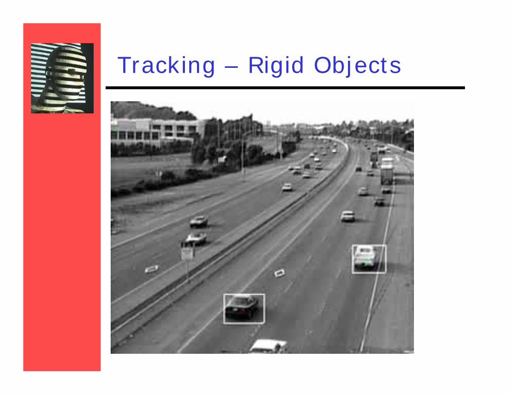
Tracking – Rigid Objects

Tracking – Non-rigid Objects

(Comaniciu et al, Siemens)

Tracking – Non-rigid Objects

7

Optical Flow:Where do pixels move to?

Optical Flow:Where do pixels move to?

)1( tI

What is Optical Flow (OF)?

Optical Flow

}{),( iptI

1p

2p3p

4p

1v2v

3v

4v

}{ ivVelocity vectors

Common assumption:The appearance of the image patches do not change (brightness constancy)

)1,(),( tvpItpI iii

Note: more elaborate tracking models can be adopted if more frames are process all at once

Optical flow is the relation of the motion field:• the 2D projection of the physical movement of points relative to the observer

to 2D displacement of pixel patches on the image plane.

9

Optical Flow: Correspondence

Basic question: WhichPixel went where?

Structure from Motion?

• Known: optical flow (instantaneous velocity)

• Motion of camera / object?

Optical Flow is NOT 3D motion field

http://of-eval.sourceforge.net/

Optical flow: Pixel motion field as observed in image.

Optical Flow is NOT 3D motion field

http://en.wikipedia.org/wiki/File:Opticfloweg.png

14

Definition of optical flow

OPTICAL FLOW = apparent motion of brightness patterns

Ideally, the optical flow is the projection of the three-dimensional velocity vectors on the image

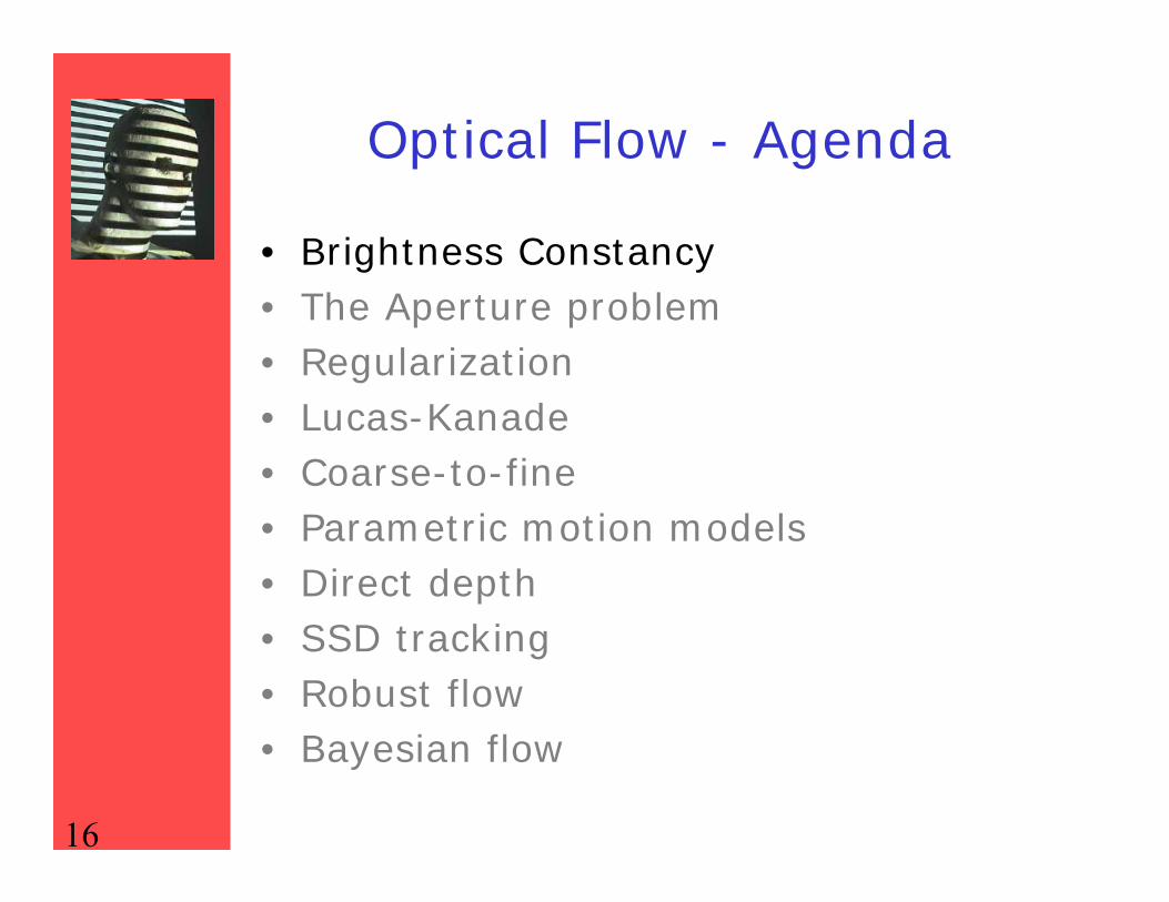
Optical Flow - Agenda

• Brightness Constancy• The Aperture problem• Regularization• Lucas-Kanade• Coarse-to-fine• Parametric motion models• Direct depth• SSD tracking• Robust flow• Bayesian flow

16

Optical Flow - Agenda


Start with an Equation:Brightness Constancy

Point moves (small), but its brightness remains constant:

, ,

→ 0Time: t Time: t + dt

Mathematical formulation (1D)

I (x(t),t) = brightness at (x) at time t

Optical flow constraint equation (chain rule):

0

tI

dtdx

xI

dtdI

),,(),( tyxItttdtdxxI

Brightness constancy assumption (shift of location but brightness stays same):

Optical Flow: 1D CaseBrightness Constancy Assumption:

)),(()),(()( dttdttxIttxItf

0)(

txt tI

tx

xI

Ix v It

x

t

IIv

0)(

txf

Because no change in brightness with time

Gary Bradski & Sebastian Thrun, Stanford CS223 http://robots.stanford.edu/cs223b/index.html 19

20

v ?

Tracking in the 1D case:

x

),( txI )1,( txI

p

Gary Bradski & Sebastian Thrun, Stanford CS223 http://robots.stanford.edu/cs223b/index.html

v

xI

Spatial derivative

Temporal derivativetI


x

),( txI )1,( txI

p

tx x

II

px

t tII

x

t

IIv

Assumptions:• Brightness constancy• Small motion 21


x

),( txI )1,( txI

p

xI

tI

Temporal derivative at 2nd iteration

Iterating helps refining the velocity vector

Can keep the same estimate for spatial derivative

x

tprevious I

Ivv

Converges in about 5 iterations22

From 1D to 2D tracking

0)(

txt tI

tx

xI

1D:

0)(

txtt tI

ty

yI

tx

xI

2D:

0)(

txtt tIv

yIu

xI

Shoot! One equation, two velocity (u,v) unknowns…

23

The aperture problem

0 tyx IvIuI

1 equation in 2 unknowns

dtdxu

dtdyv

, xII x

yII y t

IIt

Horn and Schunck optical flow equation

26

Optical Flow


How does this show up visually?Known as the “Aperture Problem”


Aperture Problem Exposed

Motion along just an edge is ambiguousGary Bradski & Sebastian Thrun, Stanford CS223 http://robots.stanford.edu/cs223b/index.html

How does this show up visually?Known as the “Aperture Problem”


Optical Flow vs. Motion:Aperture Problem

Barber shop pole: http://www.youtube.com/watch?v=VmqQs613SbE

Normal Flow What we can get !!

We get at most “Normal Flow” – with one point we can only detectmovement perpendicular to the brightness gradient. Solution is to takea patch of pixels around the pixel of interest.

Recall: Aperture Problem

Aperture Problem and Normal Flow

• let (u’, v’) be true flow

• true flow has two components: – Normal flow:

d– Parallel flow:

p• normal flow

can be computed

• parallel flow cannot

(u’,v’)dp

u

v

Computing True Flow

• Schunck• Horn & Schunck• Lukas and Kanade

Possible Solution: Neighbors

Two adjacent pixels which are part of the same rigid object:• we can calculate normal flows vn1 and vn2

• Two OF equations for 2 parameters of flow:

. 0

. 0

Schunck: Considering Neighbor Pixels

Schunck: Considering Neighbor Pixels

Jepson, Toronto: http://www.cs.toronto.edu/pub/jepson/teaching/vision/2503/opticalFlow.pdf

Cluster center provides velocity vector common for all pixels in patch.

42

Optical Flow

• Brightness Constancy• The Aperture problem• Regularization: Horn & Schunck• Lucas-Kanade• Coarse-to-fine• Parametric motion models• Direct depth• SSD tracking• Robust flow• Bayesian flow

43

Horn & Schunck algorithm

44

Additional smoothness constraint (usually motion field varies smoothly in the image → penalize departure from smoothness) :

,))()(( 2222 dxdyvvuue yxyxs OF constraint equation term(formulate error in optical flow constraint) :

,)( 2 dxdyIvIuIe tyxc minimize es+ec


45

Variational calculus: Pair of second order differential equations that can be solved iteratively.


46

Horn & Schunck algorithm Δ 0

Δ 0

Δ , , ,Δ , , ,

Approximate Laplacian by weight averaged computed in a neighborhood around the pixel (x,y):

Rearranging terms:0

0

2 equations in 2 unknowns, write v in terms of u and plug it in the other equation

47


2 equations in 2 unknowns, write v in terms of u and plug it in the other equation

48

The Euler-Lagrange equations :

0

0

yx

yx

vvv

uuu

Fy

Fx

F

Fy

Fx

F

In our case ,

,)()()( 22222tyxyxyx IvIuIvvuuF

so the Euler-Lagrange equations are

,)(,)(

ytyx

xtyx

IIvIuIvIIvIuIu

2

2

2

2

yx

is the Laplacian operator


49

Remarks :

1. Coupled PDEs solved using iterative methods and finite differences

2. More than two frames allow a better estimation of It

3. Information spreads from corner-type patterns

,)(

,)(

ytyx

xtyx

IIvIuIvtv

IIvIuIutu


Discrete Optical Flow AlgorithmConsider image pixel

• Departure from Smoothness Constraint:

•Error in Optical Flow constraint equation:

• We seek the set that minimize:

i j

ijij cse )(

])()(

)()[(41

2,1,

2,,1

2,1,

2,,1

jijijiji

jijijijiij

vvvv

uuuus

2)( ijtij

ijyij

ijxij IvIuIc

}{&}{ ijij vuNOTE: show up in more than one term

}{&}{ ijij vu

),( ji

Discrete Optical Flow Algorithm• Differentiating w.r.t and setting to zero:

• are averages of around pixel

e0)(2)(2

kl

xkltkl

klykl

klxklkl

kl

IIvIuIuuue

0)(2)(2 kl

ykltkl

klykl

klxklkl

kl

IIvIuIvvve

klkl uv &

klkl uv & ),( lk),( vu

klxkl

yklx

klt

nkl

kly

nkl

klxn

klnkl I

IIIvIuI

uu])()[(1 22

1

klykl

yklx

klt

nkl

kly

nkl

klxn

klnkl I

IIIvIuI

vv])()[(1 22

1

Update Rule:

Horn-Schunck Algorithm : Discrete Case

• Derivatives (and error functionals) are approximated by difference operators

• Leads to an iterative solution:

yn

ijnij

xn

ijnij

Ivv

Iuu

1

1

)(1 22yx

tn

ijyn

ijx

IIIvIuI

neighbors of valuesof averages theare , vu

Intuition of the Iterative Scheme

u

v (Ex,Ey)

Constraint line

(u,v)

),( vu

The new value of (u,v) at a point is equal to the average of surrounding values minus an adjustment in the direction of the brightness gradient

Horn - Schunck Algorithm

Example

http://of-eval.sourceforge.net/

Results

Optical Flow Result

60

Horn & Schunck, remarks

1. Errors at boundaries (smooth over)

2. Example of regularization(selection principle for the solution ofill-posed problems)

Results of an enhanced system

Resultshttp://www-student.informatik.uni-bonn.de/~gerdes/OpticalFlow/index.html

Resultshttp://www.cs.utexas.edu/users/jmugan/GraphicsProject/OpticalFlow/

64

Optical Flow


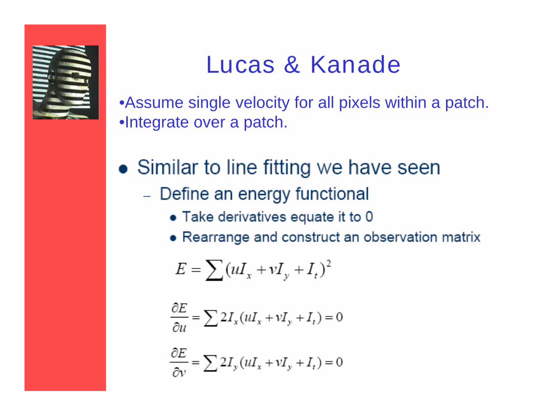
Lucas & Kanade•Assume single velocity for all pixels within a patch.•Integrate over a patch.

Lucas & Kanade

68

02),(

02),(

tyxy

tyxx

IvIuIIdv

vudE

IvIuIIdu

vudE

Discussion• Horn-Schunck: Add smoothness constraint.

• Lucas-Kanade: Provide constraint by minimizing over local neighborhood:

• Horn-Schunck and Lucas-Kanade optical methods work only for small motion.

• If object moves faster, the brightness changes rapidly, derivative masks fail to estimate spatiotemporal derivatives.

• Pyramids can be used to compute large optical flow vectors.

Iterative Refinement(Iterative Lucas-Kanade)

• Estimate velocity at each pixel using one iteration of Lucas and Kanade estimation

• Warp one image toward the other using the estimated flow field(easier said than done)

• Refine estimate by repeating the process

Reduce the Resolution!

73

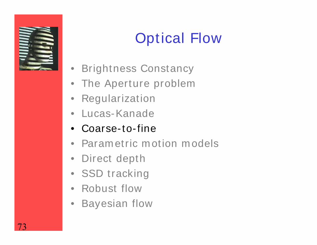
Optical Flow


Revisiting the Small Motion Assumption

• Is this motion small enough?– Probably not—it’s much larger than one pixel (2nd

order terms dominate)– How might we solve this problem?

image Iimage H

Gaussian pyramid of image H Gaussian pyramid of image I

image Iimage H u=10 pixels

u=5 pixels

u=2.5 pixels

u=1.25 pixels

Coarse-to-fine Optical Flow Estimation

image Iimage J

Gaussian pyramid of image H Gaussian pyramid of image I

image Iimage H

run iterative OF

run iterative OF

upsample

.

.

.

Coarse-to-fine Optical Flow Estimation

Video Segmentation

Next:Motion Field

Structure from Motion

Motion Field

X

Y

or

ir

'f

• Image velocity of a point moving in the scene

Perspective projection:Zf

o

o

oi

rZr

rr

ˆ'1

22 ''

ZrZvr

ZrrZvvZrrv

o

oo

o

ooooii ff

dtd

Motion field

tov

tiv Scene point velocity:

Image velocity:dtd o

orv

dtd i

irv

ZZ

Optical Flow I - Scientific Computing and Imaging...

Documents

Transcript of Optical Flow I - Scientific Computing and Imaging...