openSAPIntroduction to Software Development on SAPHANA

WEEK 2, UNIT 1

0:00:13 Hello, and welcome back to week two of this openSAP platform presentation of introduction tosoftware development for SAP HANA. In the first week, we saw a lot of architectural information,getting started, installing the SAP HANA studio and configuring it, and setting up a very simpleHello World. Now, in week two, we'll begin our journey of building a sizable application. We'llbuild this one layer at a time, just as you would build a real application. We're going to start atthe lowest layers of the application foundation—building out from the database schema,database tables, simple views and other database artifacts in the catalog—and eventuallyapplying HANA-specific views and other data-intensive logic on top of our core data model.

0:01:05 So for week two, unit one, we're going to start with our empty HANA database and begin bycreating both schemas and a base database table.

0:01:19 Of course HANA is an SQL-compliant database, and you can create artifacts using SQL. Youcan go to the SQL command prompt and type Create Table, for instance. But when you createobjects directly via SQL, you don't have all the benefits of creating them in the SAP HANARepository. Creating them via SQL means that the SQL itself needs to be saved and re-executed on each target system where you want that content to be created.

0:01:51 That's why in the SAP HANA world, we introduce the concept of the repository. The repositoryallows us not only to store source code and other development artifacts, as we saw in weekone, but it can also store the definition of catalog artifacts. And when we store things likeschema definitions and table definitions in the repository, and we activate them, the activationprocess will generate the necessary SQL statements to either create or update the existingobject in the catalog. This allows us to have a little bit of a separation between what is possiblewith SQL and what we could define in HANA specifically. It also begins to provide almost a littlebit of a data dictionary that provides additional services over and above what you can definewith SQL. As you'll see in some of the examples that we'll do throughout this week, we'll createobjects, but we'll also create relationships between objects using semantics that SQL simplydoesn't have. But at the same time, we won't break compatibility with SQL. Everything that we'llgenerate in the repository will still have a SQL catalog representation. And of course, if you'reporting an existing application from another database, you're still welcome to use SQL to createthose artifacts.

0:03:19 Some of the additional benefits that we have if we create the objects in the SAP HANARepository: The repository gives us our object management, our versioning, and our transportmechanisms. So we can have multiple versions of objects, where if you created them directlywith SQL, you wouldn't have any versioning except maybe on the SQL CREATE statementsthemselves. We have transport capabilities. We have the ability to package everything up—allparts of an application, from the schema, the tables, the logic, the services, and the user

This document contains a transcript of an openSAP video lecture. It is provided withoutclaim of reliability. If in doubt, refer to the original recording on https://open.sap.com/.

Page 2 Copyright/Trademark

interface—into a single file that we call a “delivery unit”. This file can then be given to customersor partners, and is very easy to install in the target system. Much later in this material, we'll talkmore extensively about lifecycle management and transport management and you'll see howthat comes together. But for now, know that that's part of the power and the reason that wewould want to use the SAP HANA Repository.

0:04:20 With the SAP HANA Repository, we also have patching mechanisms built in. So maybe youonly want to deliver the objects that have changed during a certain time period. Well, therepository tracks all the changes and allows you to create these delivery units with just theobjects that have been changed.

0:04:38 The SAP HANA Repository also has built-in capabilities for supporting translation, morespecifically, supporting multiple language versions of text strings. So, for instance, in a regularSQL catalog, you have the possibility to have column headers, but nowhere to do language-dependent descriptions of those column headers. The SAP HANA Repository adds thatadditional feature.

0:05:03 Finally, the SAP HANA Repository really supports server-side development using standardEclipse tools and check in and check out, as we saw in the earlier week. This allows bettercontrol over your artifacts, better team coordination, than what you would have if you were justwriting SQL directly.

0:05:23 Just to help you visualize, once again, what the SAP HANA Repository contains: It contains allof our data artifacts, meaning the definitions of all of our catalog objects, our tables, our views,and so forth; as well as the data-intensive logic in the form of SQL script; all of our control flowlogic, being our REST-based services, our server-side JavaScript; and our presentation logic.So the raw HTML and JavaScript libraries which HANA will serve out acting as a static Webserver are also stored in the HANA Repository.

0:06:01 Now that we've established that we want to use the HANA Repository for creating all of ourartifacts, let's look at some of them that we will create in this unit. Of course, we have a varietyof catalog artifacts that can be created, either via SQL or via the repository. This includes theschemas, which is a grouping of all of the catalog artifacts, so it is the parent object. As you seehere in this screenshot, we have a schema named SAP_HANA_EPM_DEMO. Inside thatschema, grouped inside there, we have a variety of other development artifacts, such as tables,SQL views, sequences, and procedures, just to name a few.

0:06:49 The schema is a mandatory database object; all database objects have to belong to a schema.So before we can begin to really develop anything, we have to establish our schema. Theschema then contains all the other catalog artifacts. It will help control access to these artifacts.We can create our roles later. You'll see where we grant access to a particular schema, andthen objects within that schema inherit those authorizations. So not only is it a groupingmechanism, but it's an authorization control mechanism as well.

0:07:27 To create the schema, we need only create another file in our project. This time, we'll use thesuffix .hdbschema. So let's go ahead into the system and create this now. I'll continue using theproject that we started in week one, with our simple Hello World example, and I'm going tocreate a subfolder inside this package named Data. I do this because I want some way toorganize and separate out the different layers of my application. So I'm going to put all of mydatabase catalog object definitions in this Data folder. Later, I'll create a Services folder to holdthe REST-based services. I'll separate out the user interface content. You'll see, once I committhis, that if I go back to the Systems view, and I now look into my content folder, you'll see that

Page 3 Copyright/Trademark

this Data folder has been created as a package on the server side. Earlier, we saw howpackages become folders on the client side, but the reverse is true as well. If we create a folderinside our project, it will become a package on the server side once it's committed.

0:08:59 This data is now ready for our schema file. So I'll just say New –> File and I will name the filethe same as what I want to name the schema itself: WORKSHOPA_00.hdbschema. Onceagain, because you don't want to watch me type, I will cut and paste the content. Now what wehave created here as part of the learning workshop is many templates. Often we are going tocut and paste from existing templates, or maybe we have some code fragment that we want toinsert into our project. We actually have a Web site built in SAP HANA, running out of our HANAdatabase, that has all of our exercises grouped together and all of the code templates and codesnippets that we need already here, ready for us to cut and paste. For instance, my syntax formy schema is all ready to insert. Just need to make one little change there. Schema name =WORKSHOP. Then I just correct the notation: WORKSHOPA, group number 00.

0:10:34 I'll save that. I will commit, and then I will activate.

0:10:46 At this point, the activation has created the schema inside the catalog on the server side. Yousee it already here, WORKSHOPA_00. It has nothing in it yet, but we are now able to createadditional database artifacts that will live inside this schema.

0:11:12 Here we simply see a slide, if you need it for your reference: the syntax that you saw that I justinserted into my .hdbschema file to create the schema.

0:11:24 The schema is really a very straightforward artifact. It's just a name that gives a grouping toother database artifacts. Now let's move on to something that's a little more interesting, as wellas a little more complex, which is the creation of database tables.

0:11:41 When we create tables in the repository, we'll still create them inside of a schema. But you'llnotice, in this screenshot, the listing of the names of the tables. I don't just have a table namedAddress and a table named Business Partner and so forth. It has a string on the front of it,sap.hana.democontent.epm.data, and then two colons. That first part is the package hierarchyof where the .hdbtable file was placed. Here we're applying the semantics of the repository, andthe name of the package hierarchy really becomes a namespace as well. Remember, I saidthere were several different uses for the packages. We've really only seen them used as afolder structure. They also become a namespace. This way, we could have multiple tablesnamed Address, even in the same schema, and as long as they were coming from differentpackages they would remain unique.

0:12:44 The repository representation of the table is also very powerful, because once I've activated itand generated a table, maybe I come along and I add a new column to that table. I don't have towrite the DROP TABLE or the MODIFY TABLE statements. The system, when I activate the.hdbtable file, will analyze the new state of the table and the current state in the catalog andgenerate the necessary commands to adjust the table. The system will always try to maintainthe data that's in that table as well. As long as you don't change the core data types of acolumn, you won't lose any of the data during those modification operations.

0:13:29 Now let's create a table, as well. It's a very similar concept. We'll create another file. This time,we'll use the file extension .hdbtable.

0:13:45 I return to my project explorer. I go to my Data folder and say New –> File. I want to create aheader table. I just need to make sure that file extension is .hdbtable. Once again, I'm going to

Page 4 Copyright/Trademark

cut and paste because this one has a little more syntax to it and I will explain some of this toyou. Just a moment...let's get it cut and pasted in here. Add our target schema that we justcreated.

0:14:29 What we're defining here is we're telling it the schema that we want to create the table within,giving it the same target schema that we just created in the previous step. Then we need to tellit what type of table this is. Remember that HANA can support both row- and column-baseddata, although column should really be your default approach. It's going to give you the bestperformance for large amounts of data. Row-based tables would really only be applicable if youhave a small number of rows (a small number of records) but a large number of columns andyou have the tendency to select them all (or need to select them all) at once. This is generallyonly used in, say, configuration tables. Almost all of your transactional data, your master data,should all be organized in the column store.

0:15:24 Then you notice that we can add a table description. This is one of the text strings that can bemade language-dependent. Then we list our columns. We list the column names, their datatypes, their links, and a comment on the columns as well. Not that drastically different than thesame syntax that you would type in a CREATE TABLE statement. In fact, if you already have anexisting CREATE TABLE statement, you can often just cut and paste it into the .hdbtable fileand do some simple formatting to turn it into this JSAN-based syntax.

0:16:02 Finally, we list the primary key of the table. I save, and now I will activate. Notice this does acommit, then it does an activation, and that table would now be created within my schema.

0:16:25 And there we have it. And notice it's not just header as the name of the table. It'sworkshop.sessiona.00.data, as part of the package name added to the beginning of the tableitself. One thing that you might notice if I try to actually access this table and view any of thedata in it or view the structure of it: It's telling me that my user has no privileges tothis table. Youmight think that that's odd, because I just created this table, but in fact, everything that's createdin the repository is not owned by the developer who created it. It's all owned by the system usersysrepo. This is actually a good thing because it removes the fact that particular developers ownobjects just because you created them. Everything is centrally created and centrally owned, andthat makes it much easier to manage over time. It does mean that before I could go forwardworking with any of the database objects that I generated, we'll have to create a role and grantthat role to my user. But that's something that will come in a little bit later unit in this week.

0:17:37 Just to close out, we have the slide here that shows you the syntax of the .hdbtable format,identical to the example that I just showed you in the system. With that, you've seen how simpleit is to create both schemas and database tables within the schemas. In subsequent units in thisweek, we will look at additional database objects, as well as building up views and other data-intensive logic on top of the table and the schema that we've created in today's unit.

Page 5 Copyright/Trademark

WEEK 2, UNIT 2

0:00:13 Hello, this is week two, unit two: Sequences and SQL views.

0:00:18 In this section we’ll continue our discussion of creating catalog objects in the HANA Repositoryand we’ll look at two additional objects which we can create in the repository, and that would besequences and SQL views. We’ll discuss a little bit about what each of these objects are andhow they can be created in the HANA Repository.

0:00:40 First let’s take a look at database sequences. A database sequence is basically a incrementinglist of numeric values.

0:00:49 It’s very similar to a number range, if you’re familiar with that concept, perhaps from otherdevelopment environments.

0:00:59 It allows you to basically have a unique key or even a non-key field that you will auto-incrementas you insert new records into the database.

0:01:12 And this can be both ascending and descending. It has a lot of uses both for the generation ofkeys, but also for the coordination of data between JOINs in two different tables.

0:01:29 Therefore it’s pretty commonly used when you’re creating applications that use transactionaldata. It can be very useful in the generation of keys in that transactional data.

0:01:41 So let’s have a look at how we can create this sequence now inside the HANA Repository.

0:01:48 So, we’ll switch over to the system. The process is very similar to what we saw in the previousunit when we created our tables and our schemas.

0:01:58 We’ll continue to work in the data package and I’ll create a new file: OrderID.

0:02:12 And the file extension I’ll use will be .hdbsequence. So hopefully you’re starting to see a patternin that most of the file extensions begin .hdb, for HANA database, and then it’s the name of theobject, such as schema, table, sequence.

0:02:33 And inside this OrderID.hdb sequence file, I’ll need to insert a little code snippet here. Again youdon’t want to watch me type, so I’ve prepared a template.

0:02:45 The template, there’s not a whole lot to it, you have to give it the schema name that you wantthe catalog object to be created within, just like we had to do with our table

0:02:59 So, put that into the workshopa.00.schema.

0:03:06 You give it a starting number. We don’t have to specify a starting number, we would start withone if we didn’t specify a number, but we want to begin our number range at a certain point andallow it to increment up from there.

0:03:21 And then the last property we have in the HDB sequence file is this depends_on_table. This iswhere we start to see some additional functionality of creating the objects in the repository, asopposed to creating them directly in the catalog.

0:03:36 If I were to create a sequence with SQL statements directly in the catalog, there would be noway to specify which table utilizes the sequence.

Page 6 Copyright/Trademark

0:03:46 But because we’re creating it in the repository, we’re creating this cross-reference in therepository with this depends_on_table entry. The system will know that if I drop the table it canprompt me to say that there was a sequence connected to this table, and do you want to dropthis as well, or any other kinds of adjustments when we have these dependencies betweenobjects the system can correlate that relationship and warn us or alert us when we may need toact on the related object as well.

0:04:18 So here I’ll simply supply the name of our table. So we’ll put this in sessiona.00.data and then itwas header.

0:04:32 Now notice that I don’t have to specify the .hdb table, I’m actually specifying the name of thetable as it exists in the catalog, therefore it just ends with the header.

0:04:46 So I’ll go ahead and save this and I’ll activate and it’s now successfully created my sequence.

0:05:11 Now going back to our slides for just a moment, once the sequence has been created you cansee here a little code sample of how it might be used inside of an insert statement.

0:05:24 So if I was inserting a new record into the header, in my header table that we created in theprevious unit there is a Purchase Order ID field that I need to put a value in.

0:05:38 Well, if I’m inserting a new record, I just want to increment the sequence; therefore I use thereference to the sequence .nextvalue directly in the source code in the INSERT statement itself,and that will cause the sequence to generate the next number and insert that into the record.

0:05:56 So you see a little about how easy it is to use the sequence inside of our SQL statements.0:06:02 A couple of the other key words that are available with the sequence in addition to the start_with

that we used to begin the sequence at a certain level, you can have the nomaxvalue,nominvalue, which means that the sequence can run to the end of the number range.

0:06:24 We can also have cycles, true or false. This would mean that when you fill the sequence you getto the end of the definition, you know, 9 million, 900 thousand, 999 perhaps, if cycles=true thenthe sequence will automatically start back over at 1.

0:06:46 But maybe you don’t want it to start back over because those records have already beeninserted into the database, so quite often you’ll say cycles=false.

0:06:56 And then we have the depends_on_table, which I showed you in this exercise, but you can alsohave a depends_on_view as well.

0:07:07 Now, moving on, we’ve seen how to do the sequence. Now let’s talk about another databasecatalog object ,and that would be the SQL view.

0:07:18 A SQL view is a basic join between two or more tables, and sometimes you want to define thatjoin in the catalog and have it as a reusable object.

0:07:31 A little bit later in this week, we will talk about the HANA-specific view types that are much morepowerful and have the capability to have calculated fields and measurements and aggregatesand all these sorts of things.

0:07:45 What we’re talking about here is really the basic SQL view, just what you could define with

Page 7 Copyright/Trademark

regular ANSI SQL, or of course anything you can put in a SQL statement with the GROUP BY,summation, those sorts of things can be built into the view and not the more powerful HANA-specific features.

0:08:02 So sometimes this type of view is good enough that you want to create it without using themodeling tools and therefore we have the ability to create SQL views directly in the catalog.

0:08:16 So the process for creating these via the repository is nearly identical to the process we’ve seenfor the other artifacts so far.

0:08:26 So let’s go back into the system and go to our project and the data package and we’ll createanother new file.

0:08:40 Ordersext is the name of my view and then the file extension: .hdbview, following the patternthat we’ve seen all along.

0:08:52 So I have another text file ready to be edited,. I’ll bring my template in for the view, and thenwe’ll talk about what this code template is doing.

0:09:07 So there’s a little bit more to this code template but it’s really not all that complex. We have tosupply the schema, very similar to our other artifacts.

0:09:19 And then we have the query and this is literally the SQL statement that defines the JOINcondition, so we have to supply the tables so we’re saying which fields we want to select, wehave to supply the tables for the FROM condition

0:09:41 So from my schema and then sessiona.00 and I want to join the header table that we created inthe unit yesterday and join that together with the item table, which I created offline because theprocess was the same as creating the header table. There was no reason for you to watch medo the same process again

0:10:12 But now that I have a header and an item table I’m able to join those on my order ID and I’llorder the results by order ID.

0:10:21 So a pretty typical SELECT statement with a JOIN condition, I could have written the selectstatement over in the SQL console and simply cut and pasted it into this file. In fact that's how Ioriginally built this, as I wanted to test it and make sure that the join worked correctly.

0:10:39 And only once my select statement for the join worked, then I cut and pasted it into this editor.

0:10:46 Now one thing that you’ll note is the use of quotes so anywhere that you’ll use a quote insidethe select statement it has to be escaped because this actually is going to be an JSON notation,the file itself, even though it looks like just a fragment here, the headers for the rest of the JSONare inserted when you activate the file.

0:11:10 Therefore the query is a comment in and of itself and there isn’t any real parsing of the innerprocessing of this query, the SELECT statement.

0:11:20 And because it’s all one big string constant from the beginning of the select all the way down tohere, we have to take any quote marks that appear inside the SELECT statement and escapethem, meaning we had to put this back slash in front of the quote, that’s why you see that usedall throughout here.

Page 8 Copyright/Trademark

0:11:43 Now the last thing that we have is we have a depends_on_table in here as well, very similar tothe same concept from the sequence.

0:11:53 I’ll just adjust my group number and you’ll see that we’re now defining that this view nowdepends upon the Header table and the Item table.

0:12:03 And once again, that has value over and above what we would have if we had generated theview directly in the catalog. Now we have a relationship between the base tables and the viewthat sits on top of those tables and we can check that during activation and other operations thatwe might perform under this table to see if we’ve invalidated our view or need to make someadjustments to it.

0:12:28 So we go ahead and save my view and we’ll activate it.

0:12:38 And it has now successfully been created. And if I go back over into my catalog display, I nowsee this view here. Now of course, once again, I can’t test any of these objects yet.

0:12:58 Remember, we spoke in unit one about how these objects are all generated by the user IDsys_repo and therefore that is the user who owns these objects. It’s not until the next unit wherewe’ll create roles and then grant those roles to our user so that they can insert some data intothese tables and be able to test the views and sequences.

0:13:18 So hopefully you’ve seen a continuation of our concept of creating catalog objects in the HANARepository and seen how similar all these objects are, that it’s only a little difference in thesyntax of the individual files in order to create the various types of database objects.

Page 9 Copyright/Trademark

WEEK 2, UNIT 3

0:00:13 This is week 2, unit 3: Authorizations. In this unit, we will look at how we can create roles andthen grant those roles to our user ID.

0:00:23 As we’ve seen in the previous units, we’ve been creating a lot of catalog objects via the SAPHANA Repository.

0:00:32 And as we’ve created all these objects, you’ll remember that we didn’t immediately haveauthorization to those objects.

0:00:39 Whenever we create something in the content repository, the user that does the activation isactually the sys_repo user; therefore, that is the user who has ownership of those objects andinitially the only user who has access to those objects.

0:00:55 And no one can log on as sys_repo, as it’s a built-in system user. Therefore pretty quickly in thedevelopment process, you need to start creating your roles and granting those roles to youruser ID before you can move much further.

0:01:08 We really can’t even really see the details of the objects we’ve created so far in the catalog norcould we insert any data into them or do any initial testing before we have access to them

0:01:22 So let’s have a look at how we can create roles inside SAP HANA.

0:01:27 So everything around roles and the granting of roles to the users is all done within the securityfolder in the Modeler view.

0:01:39 Up until HANA 1.0 SP5 we created roles only via this Security Roles folder.

0:01:49 And there was this form-based editor that popped up to let you maintain the roles. I’ll show youthat in the system in just a minute. But one of the limitations of these roles was that it wasn’t agreat tool to use to move roles from one system to another.

0:02:05 And this older form of role , they’re the ones you still see in the system, generally all upper case,and they don’t have a package path on the front of the role name.

0:02:15 So that’s what we would call default roles or built-in roles or sometimes referred to as modeler-created roles.

0:02:26 And this is some of the roles you see that are delivered by SAP, the default roles or the built-inroles, such as CONTENT_ADMIN, the MODELING, and the PUBLIC, and often you’re usingone of these base roles to build your users, they would have one or more of these base defaultroles but then you need to create roles for your particular content that you would create.

0:02:47 You create addition views and tables as we’re doing in this learning exercise and we need togrant authorization to be able to work with those objects. Therefore we’ll create those roles inthe repository.

0:03:01 Now this is new as of HANA 1.0 SP5, the ability to create roles in the repository. And this givesus a way to transport the role along with all the other development content because when wecreate them in the repository, it has all the benefits we talked about with objects created in thecontent repository.

Page 10 Copyright/Trademark

0:03:22 Now the roles created in the content repository always have the package path on the front oftheir name. Very similar to what we’ve seen with all the catalog objects, the tables and the viewswe’ve created so far, how they get their package path added to the beginning of their name aswell.

0:03:39 So let’s go into the system and I’m here in the SAP HANA Systems view and from the securityfolder I have the ability to view users. And we’ll use this a little bit later once we’ve created therole to see it granted to our user ID.

0:03:59 But we can also see roles, some of the built-in roles like MODELING, the MONITORING, andPUBLIC like we talked about. And you see some other roles here that have been created in thecontent repository. You know that because we have the package path on the front of the name.

0:04:18 Now if we look at one of these roles, we see the options that were possible in the older form-based editor. Inside a role we can add subroles, so basically we have an inheritance model so Ican have other roles that are part of a composite role and inherit all the capabilities of the rolesthat have been granted to this role.

0:04:44 We have a tab that will show us if this role we’re editing has been granted a part of any otherrole.

0:04:51 We have the ability to add SQL privileges. So here we can list any catalog object, such as aschema, a table, or a procedure, and then control its various options and abilities to executeSELECT INSERTs and get rather granular on the options that you have or that you’re grantingvia the role.

0:05:12 Analytic privileges is something that we’ll talk about later in this week.

0:05:17 Then we have system privileges. These are core system privileges such as the ability to dobackup and recovery, export, import, that you can also grant to a role

0:05:27 Then finally we have to have the ability to control the authorizations on packages, at thepackage level, so in the content repository not every user ID needs visibility to all packages.

0:05:41 Nor would they necessarily need edit or activate capabilities. So you can grant the ability tocontrol what people can do inside a package as well.

0:05:56 So we’ve seen a little bit about the basics of a role in SAP HANA. Now let’s begin to create ourrole for the workshop content that we’ve created so far.

0:06:07 And we’re going to do this and the process is going to be very similar to what we’ve done so farwith all the catalog objects we’ve created in the HANA Repository. We’ll create a file and havean extension .hdbrole. There’s actually a little wizard for the role that will help us generate thefile so we won’t have to specify the file extension for this one.

0:06:29 So let’s go ahead into the system and start the process of creating our role.

0:06:34 So I’ll go to the Project Explorer and inside our Data tab I will say New—> Other and I will usethe role wizard, I could have still used New—>File and given it the file extension myself, and Iwould have had a blank editor.

0:06:52 But as you see here if I use the wizard and say New—>Role, I don’t have to specify the file

Page 11 Copyright/Trademark

extension, I just put in the file name of the role: workshopUser, and say Finish. It actually insertsa little bit of a template for me.

0:07:08 I do have to go in and complete this template, I have to add the full package name,workshop.sessiona.00.data. And you notice that syntax error, that I hadn’t completed that “todo”, went away from red to grey ,so I know that I’ve corrected that problem.

0:07:30 And now you don’t want to watch me type any more than you have to, so I’m going to cut andpaste in the two things that we’re going to grant inside this role.

0:07:45 So here we want to grant SELECT on our schema, so we just correct this and put in the fullname of our schema, workshopa.00.

0:08:05 So that’s our schema so we can grant objects at both the catalog level, in this case we’rereferencing the schema as its catalog name, we’re saying grant the SELECT option on thatschema.

0:08:18 We can also reference objects by their repository ID, and this works for all kinds of objects. Wecould grant authorization to a table or a view and give it its repository representation name,meaning the full package path.

0:08:36 Or we could reference the catalog object directly. Now the second part of this is one wherewe’re going to reference a repository object and this is actually an application privilege.

0:08:48 This is a new type of object that was introduced in HANA 1.0 SP5, and you can actually notmaintain the application privileges in the old form-based editor. The only way to maintainapplication privileges is in the .hdbrole editor that you see here.

0:09:06 And an application privilege is something that we’ll talk about a little bit more later on, because ithas to do with how we control authorization inside XSJS services, the server-side JavaScriptservices, and our own database REST services.

0:09:23 So something that has to do with the programming model that we’ll get to later, for now, all youhave to know is that I defined these privileges in advance, I actually created another file herenamed .XSprivileges and I’ve said that we’re going to have two levels of privileges: Basic andAdmin.

0:09:41 Now, we haven’t connected that up to anything so it doesn’t really control anything yet, but you’llsee that later when we start creating our services how we can assign these applicationprivileges to particular services.

0:09:55 For now we just want to go ahead and grant the Basic privilege to our User role, my User role isgood.

0:10:02 Now in a typical application, you’re probably going to want a couple of different levels ofauthorization, in this case in our exercise we want a basic User role.

0:10:16 And they’ll have SELECT against all of our tables, but then we want to create an Admin role,and that Admin role would have also have CREATE, DELETE, DROP, all these additionalauthorizations and that’s actually what we’ll give to ourselves as developers. because we needmore ability going against these tables as we develop against them.

Page 12 Copyright/Trademark

0:10:36 So let me create another role and that I’m naming it right.

0:10:47 So workshopAdmin is the name of the role we want to create.

0:10:55 So once again I’ll correct the package path.

0:11:05 And what you’ll see here is that we’ll use the inheritance concept because I’ll say that the Adminrole extends the User role.

0:11:22 And this way we won’t have to redefine everything that was in the User role, so we’llautomatically get the select on our schema and we’ll need to only add the additional capabilities.

0:11:36 And this is nice, this is a fairly simple role so we probably wouldn’t have to do the inheritance,this was really simple enough, I’m re-supplying the SELECT on the schema anyway.

0:11:49 But if you had very complex roles and maybe you just want to add one or two minor additionalcapabilities with an Admin role over a Basic role, that’s where the inheritance becomes reallynice and really useful.

0:12:06 And you notice that the application privilege that this role will get is the Admin one.

0:12:11 So let's go ahead and save and then we’ll activate both these objects at once.

0:12:22 And I’ve done everything correctly, so there we are, we have active roles. And if I return to theHANA Systems view and refresh my role list, now you’ll notice that I have an Admin role and aUser role and I can see the details of these roles.

0:12:39 So you can see that the User role is part of the Admin role. Uou can see the SQL privileges thatwe’ve granted here, that the User has SELECT on the schema, whereas the Admin user willhave more authorizations to that schema.

0:13:02 So we see a little bit about what we can do here inside our role in addition to granting privilegesat the schema level, as we’ve done here. At the application level there’s a variety of other thingsthat we could grant. This is really just scratching the surface.

0:13:17 You can refer to the full syntax of the .hdbrole inside the developer's guide that is availableinside HANA studio or available at help.SAP.com and you can see how you can grant additionalprivilege types on all kinds of catalog objects or repository objects.

0:13:38 Now the role itself is owned by sys_repo as well, so we don’t have authorizations directly to thisrole, nor could we initially have authorizations to grant this role to ourselves.

0:13:51 Right now, only sys_repo has the authorization to grant this role and since nobody can log on assys_repo, well then the role wouldn’t have been very useful if we didn’t have a workaround.

0:14:04 Luckily what SAP provides is a SQLScript stored procedure. and when you define a SQLScriptstored procedure, as we’ll see later, a stored procedure can run as the user who created it.Therefore we can run this grant activated role procedure and when you run this role it will run assys_repo therefore it will have the authorization to grant any role that sys_repo has created toour user ID.

0:14:37 Now a little comment about this, this ability to run the GRANT_ACTIVATED procedure, it’s a

Page 13 Copyright/Trademark

very powerful procedure. Most developers in most systems will not have the authorization to runthe GRANT activated role. Only a powerful system user would have this role.

0:14:56 So obviously if a developer had the ability to create roles and the ability to grant any of thosecreated roles, they could give themselves any authorization

0:15:04 Therefore this is normally a process that at this point the developer would have to go to thesystem administrator, security administrator, and ask them to grant their new role to their userID.

0:15:17 So let’s just look real quickly at the process for running this GRANT. If I open the SQL consoleand then I can type in the statement to grant the role.

0:15:33 I’m not going to type, I’m going to cut and paste. This is the SQL command: this call.

0:15:40 And then we list the name of the SQLScript procedure that we want to run,GRANT_ACTIVATED_ROLE, and then we’re going to pass two parameters in.

0:15:49 One is the name of the role: sessiona.00.data::workshop admin. And then I’m going to grant thisto my user ID, my user ID being OpenSAP. And I can execute this and now this role has beengranted to my user. I can go back to the User folder and verify this. If I look at my user ID, I cannow see that this workshop::admin role has been added to my user ID.

0:16:30 This also means I can also go back to the catalog and I can go to my tables, for instance. If youremember earlier in the previous unit when I tried to display the details of the table, I actually gotan error message that I wasn’t authorized. Now I’m authorized to see the details. I’d be able toinsert data, I can run the data preview—although we don’t have any data in our table yet so it’snot going to return any data—but it doesn’t give me any authorization errors.

0:17:02 So, in this unit you’ve seen how we can create a role. Not just create it, but also create it in thecontent repository. And once we have that role created, call a special SQLScript storedprocedure to be able to grant that role to our user ID. So now we have the authorization to moveforward building more objects on top of the schema and the tables and views we’ve createdalready.

Page 14 Copyright/Trademark

WEEK 2, UNIT 4

0:00:13 Hello this is week two, unit four: EPM Demo Schema. So far we have been building on all of ourartifacts as part of our project, but in order to save time, we want to have more a complexnumber of objects, but we don’t want you to have to build all of them yourself.

0:00:33 Therefore SAP has built and delivered a demo scenario, which can be used for learning andother purposes. We’ll actually, for the remainder of this workshop, be building on top of thisEPM demo schema.

0:00:48 EPM stands for Enterprise Procurement Management, and the idea is that SAP wanted to builda demo and training learning data model that could be used across many different platforms andbe pretty reasonable as far as its design, meaning something that everyone can relate to. Itwouldn’t have too many tables or too many fields and it would be a business scenario that madesense to most everyone.

0:01:18 So we decided to focus on enterprise procurement, which basically means sales orders,purchase orders, business partners, products, and addresses.

0:01:30 It’s something that almost everyone understands; we’ve all bought or sold something at somepoint in our lives, so the idea of a sales order or a purchase order is pretty familiar even if youhaven’t worked in an ERP type scenario.

0:01:44 Now this demo schema and scenario originated in the NetWeaver world. The SAP NetWeaverworld and has been implemented in NetWeaver Java and NetWeaver ABAP, and now we’ve re-implemented it specifically for HANA

0:02:00 And in this unit what we want to do is just show you a little bit about the demo scenario, whatcontent is available, because as I said the remaining weeks and units that are available in thisworkshop will build on top of this content. And we're going to use these tables and these viewsas we build additional content.

0:02:21 So the EPM demo content basically includes a variety of objects. It has its own schema namedSAP HANA EPM demo. Inside that schema there is a variety of tables, views, sequences,synonyms, and other content that we haven’t necessary covered yet.

0:02:41 We want to look at some of the things that we have discussed and then show you things in theEPM model, because we are going to be building more content on top of this. There are severalbase tables already mentioned that we have. There is purchase orders and sales orders, thoseare the main transactional tables.

0:02:59 And then we have products, because to buy and sell something you have to have product andproduct information, as far as its size, and its description, and so forth.

0:03:08 And we have address. We also have employees, so the person who creates the purchaseorder, we have to have record of who they are. We have an address table. The address table isactually shared by our business partners and our employees.

0:03:25 And then we have a couple of behind-the-scenes tables and that’s are constants and ourmessages. And these we'll used much later when we get into creating our user interface andour services. Because what we did is we created tables to allow us to store in the databasesome reusable values that are language-dependant.

Page 15 Copyright/Trademark

0:03:50 So for instance some of the things that will appear in the user interface. We didn’t want to hard-code field labels. We didn’t want to hard-code error messages. We wanted them to betranslatable, so we can support multiple languages in our user interface. Therefore we builtsome additional tables to store that content and then we can key it by the language key.

0:04:13 And then there’s a series of other tables, I’ll show you when I get into the system, that storessome base information about currencies and about unit of measures, because we are going touse multiply currencies for our dollar amounts, for our net value, gross value, in both ourpurchase orders and our sales orders.

0:04:34 But we will also have multiple units of measure, so different types of units of measure and laterwe will be able to use the fact that we have this complex set of data with multiply currencies andunit of measures to be able to perform currency conversions and unit-of-measure conversionsinside the database, so you see how our data model is well-structured to take advantage ofsome of the capabilities of HANA.

0:04:58 Now we also have some views so we have already learned in this week that we can createsequel views, we have a similar sequel view to what we created in our demonstration earlierthat combined header and item except here it combines purchase order header and purchaseorder item.

0:05:17 We also have a set of sequences, because to insert data into most of these tables we needsome unique numeric key therefore the address ID, the employee ID, the partner ID, even thepurchase order and sales order IDs are all built as sequences and they auto-increment as weinsert data into those tables.

0:05:43 And then finally for the currency conversion and unit of measures tables, we needed synonymscreated. A synonyms is basically an alternative name for a database table. And what we neededfor the currency conversion to work correctly is we had to remove the package, the packagepath, on the front of the table name.

0:06:09 We have already learned how that when you create a table in the content repository, when itgenerates the catalog object it puts the package path on the front of the table. That creates avery long table name. That would not be compatible with the currency conversion, where itexpects a short table name. Therefore we’re able to create a synonym for the long tables andgive them a short table name basically removing the package path. So that is one option,although it is not possible to create synonyms inside the content repository. That is somethingthat can only be done currently via SQL statement and I'll actually show you the tool that we hadto introduce to generate the a synonyms after we install the EPM content into your system.

0:06:55 So let’s go over to the system now and I’ll show you some of this content we have. So here isthe SAP HANA EPM demo schema, and inside here we have our variety of tables.

0:07:15 For instance I might just do a little data preview and show you some of the purchase order datathat we have in here We have a lot of linked data between the relationships, so purchase order,purchase order ID or, for instance, the product table.

0:07:33 If we look at a preview of the product table. It has Created By, it just stores a number, so thisthen connects back to the employee record for the details of who created it.

0:07:48 Even the name and the description are really just IDs, and then they connect back to a generictext table, which contains all the text descriptions, language-keyed for all the different possible

Page 16 Copyright/Trademark

fields. This contains our product text, our address text—all the text objects that we might needacross our tables.

0:08:12 Now we also have a variety of other content that is delivered with this demo package. It’s all inyour system under SAP HANA Demo Content EPM, and it contains some artifacts which wehaven’t really talked about how we create yet, such as attributes, analytic views, calculationviews. These are all things that we will be creating throughout the rest of this e-learning seriesbut there are examples and additional content out here for all of these things.

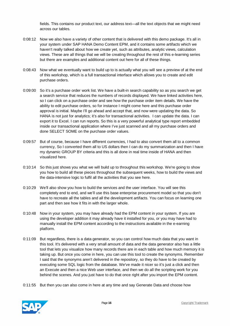
0:08:43 Now what we eventually want to build up to is actually what you will see a preview of at the endof this workshop, which is a full transactional interface which allows you to create and editpurchase orders.

0:09:00 So it’s a purchase order work list. We have a built-in search capability so as you search we geta search service that reduces the numbers of records displayed. We have linked activities here,so I can click on a purchase order and see how the purchase order item details. We have theability to edit purchase orders, so for instance I might come here and this purchase orderapproval is initial. Maybe I’ll go ahead and accept that, and now were updating the data. SoHANA is not just for analytics; it’s also for transactional activities. I can update the data. I canexport it to Excel. I can run reports. So this is a very powerful analytical type report embeddedinside our transactional application where I’ve just scanned and all my purchase orders anddone SELECT SOME on the purchase order values.

0:09:57 But of course, because I have different currencies, I had to also convert them all to a commoncurrency, So I converted them all to US dollars then I can do my summarization and then I havemy dynamic GROUP BY criteria and this is all done in real time inside of HANA and thenvisualized here.

0:10:14 So this just shows you what we will build up to throughout this workshop. We're going to showyou how to build all these pieces throughout the subsequent weeks, how to build the views andthe data-intensive logic to fulfil all the activities that you see here.

0:10:29 We’ll also show you how to build the services and the user interface. You will see thiscompletely end to end, and we’ll use this base enterprise procurement model so that you don'thave to recreate all the tables and all the development artifacts. You can focus on learning onepart and then see how it fits in with the larger whole.

0:10:48 Now in your system, you may have already had the EPM content in your system. If you areusing the developer addition it may already have it installed for you, or you may have had tomanually install the EPM content according to the instructions available in the e-earningplatform.

0:11:09 But regardless, there is a data generator, so you can control how much data that you want inthis tool. It's delivered with a very small amount of data and the data generator also has a littletool that lets you visualize how many records there are in each table and how much memory it istaking up. But once you come in here, you can use this tool to create the synonyms. RememberI said that the synonyms aren’t delivered in the repository, so they do have to be created byexecuting some SQL logic from the database. We’ve made it nicer so it’s just a click and thenan Execute and then a nice Web user interface, and then we do all the scripting work for youbehind the scenes. And you just have to do that once right after you import the EPM content.

0:11:55 But then you can also come in here at any time and say Generate Data and choose how

Page 17 Copyright/Trademark

records you want to generate. Maybe I’ll generate 2000 purchase orders and 2000 sales ordersand I'll execute this, and then you will see the data generation runs quite quickly and nicely inparallel and now I have a larger amount of records. So if you want to scale this up and you wanta million purchase orders, it’s perfectly possible to run that number up. Maybe you want toincrease your number of records, run a test, and then you can come here at any time and sayReload Seed or Reload Master Data and then reset everything back to the very small set ofdata that you started with.

0:12:38 So I hope this unit has given you an overview of the enterprise procurement demo model andgiven you some idea of the types of development artifacts that we we'll be building insubsequent weeks that sit on top of this existing demo content.

Page 18 Copyright/Trademark

WEEK 2, UNIT 5

0:00:13 This is week 2, unit 5: Single File Data Load of Comma-Separated Values. In this unit we willlook at how we can set up an initial data load into a table so that every time that the table isactivated in a new system, some base set of data will automatically be loaded into that table.

0:00:34 Now we do this by storing some additional files, including a Comma-Separated Values file intothe content repository. And then that content is linked to a particular table, and then every timethat table is activated, whatever data is in the CSV file will automatically be loaded into thecorresponding database table.

0:00:56 Now this approach is not what you would use to load massive amounts of data, so this is notmeant to replace other tools such as BusinessObjects Data Services or SLT, the SystemLandscape and Transformation tool. These are the things that you would use to move massiveamounts of data from one system to another or preload a HANA system.

0:01:20 The concept that we're going to talk about here is more for your own development and whenyou have, say, configuration tables where you want to load some initial configuration into a basetable and you deliver it into the next system.

0:01:33 It could also be used to load a little bit of seed data that you then used to generate additionaldata. In the previous unit, we saw the enterprise procurement demo model, and we used thisexact technique to deliver the base set of data in that model so that only a small amount of datais loaded into your system initially. And then we wrote the data generator that would take thebase data loaded via the CSV files and then multiply that out and generate additional randomsets of data so that you can grow the data set as large as you want. So that gives you someexamples of when you might use this technique.

0:02:13 Now to do this single file load of Comma-Separated Values, we actually need three files that willbe created in the content repository.

0:02:24 First we need the CSV file itself. Most often, you will usually use Microsoft Excel to create thedata or to cleanse the data. Perhaps you’ve extracted this data from some other system.Although more likely, if this is configuration data your probably just going to be typing it directlyinto Excel and then saving it as a coma separated value or as a CSV file.

0:02:49 Next we need the Table Import Model. This is the file that really defines the destination for thedata. It defines the database schema and table we want to insert it into every time that tablegets activated.

0:03:09 And then finally there is a third file that we need to create and that’s the table import data. Thisis what connects the CSV file and the model so it connects the target and the base data, theCSV data that we want to load into that target table. Then you might be wondering why did wecreate two configuration files in addition to the CSV file when it seems like you could justcombine this altogether into one configuration file.

0:03:37 And that’s because we actually allow you to have for the same database table, multiply CSVfiles that could be loaded.

0:03:48 And in the scenario we could have SAP-delivered files that would be in one package hierarchy,and then a customer could add their own data that they want loaded into another key space andhave their own TIM and TID file without having to change the SAP-delivered files. So it allowsyou to have multiple imports all of which get activated every time that a table is activated

Page 19 Copyright/Trademark

because the repository will go back and look up all the .tim files, all the table import modelscorrespond to a particular repository object, and automatically load all the CSVs associated withthat.

0:04:26 Now if we look at the syntax of each of these, we have a CSV file. This is typical CSV format,Comma-Separated Values properly escaped.

0:04:39 Now the one thing that you have to keep in mind is that the number of columns in the CSV filemust match exactly the target table, so you can’t have extra columns and expect them just to beignored, nor can you leave out a column. It must match exactly. That may mean even if youdon’t have data for a column, you still have to have an empty column in your source CSV file .

0:05:06 And then finally, all the data types must match. There’s not going to be any data typeconversions taking place. It will use the target data type of the table and expect that the sourcedata will match that target data type.

0:05:22 Next we have the import model, or the TIM file, so as you'll see in a second when I go into thesystem, all these will be created as files in the content repository, very similar to all the otherdevelopment artifacts we created so far but the suffix is what controls their function, and thesuffix for the import model is .hdbtim. Here we simply have to say Import CSV Files and then welist the schema and the table that we want it to be the target of our import.

0:05:59 And then finally, we have the import data file itself, and its suffix is .hdbtid for import data. In thisfile we give it the name of the CSV file or files we want to import to the corresponding TIMtarget. So we only reference the name of the .hdbtim file, and then the process will look up theactual target at runtime as it processes this file.

0:06:34 So let’s switch over to the system and let's create these artifacts so you can see what thisprocess looks like.

0:06:40 So we begin here by...we want to create a data load for our header table. Now, our header tableis transactional data. Normally you wouldn’t really be using this technique to load transactionaldata, but for the purposes for this demonstration it fits our needs, so don’t get confused by theusage that I have here.

0:07:04 So we’ll start by creating a new file. We’ll name this header.csv, and it actually opens initially inExcel.

0:07:18 And from here I could just be sure to save in Excel as a Comma-Separated Values file, but Iactually think I tell it to open with a text editor because I already have my data prepared.

0:07:32 So I’m just going to switch over to my templates and I already have a text tab delimited set, justtwo records, just enough to demonstrate the process, and I'll cut and paste that into my CSV fileand I’ll save it so the csv is all ready to go.

0:07:50 In fact I can activate it at this point. The CSV file itself doesn’t really do anything on the serverside. It just needs to be active in the repository it’s the .hdbtid and the .hdbtim file that controlthe rest of the processing.

0:08:05 So now I will create a new file and I will create the header.hdbtim file. With the .hdbtim file, welist the import table that we want to target and I just need to change the schema here.

Page 20 Copyright/Trademark

0:08:40 So there it now targets our schema, workshopa.00, and now let’s specify our table name. Andwe want to load this into our workshop sessiona.00.data::header table, and save that.

0:08:59 Now let’s create the .hdbtid file. I'll pull this from my template and here we give it the referenceto the .tim file that this one implements, sessiona.00.data::header.hdbtim.

0:09:34 And then we give it the name of the CSV file that we want to load in there,sessiona.00.data::header.csv file. Save this, and now we can activate both of these files. Bothare active. At this point, I should be able to go over to the header table and now do a datapreview.

0:10:19 And notice I have two records in here. These two records came from the CSV file and they arenow in the table. Now one thing to note, if I would change the CSV file and reactivate it, it wouldnot reload these two records. If it sees that the same keys already exist in the table, it will skipthose records and move on.

0:10:48 Now if I would add an additional record to this CSV file, it would insert that record at that timewhen I activate the CSV file. So you can trigger the insert of the data even from the CSV file. If Iwere to force reactivation on the CSV file, that would reload into the table checking for the keysas well.

0:11:11 This is part of the power of the HANA content repository that follows these relationships, theselinked relationships, so even whether I activate the table, whether I activate the CSV, or whetherI activate the .hdbtib or .tim files, all those would trigger the reload of the data.

0:11:30 So in this unit you've seen how you can create simple Comma-Separated Values files that willbe automatically loaded into a database table, and how you can assemble all this content in thecontent repository so it will be delivered along with the table.

Page 21 Copyright/Trademark

WEEK 2, UNIT 6

0:00:13 This is week two, unit six: Attribute Views.

0:00:18 In the previous units we’ve seen how we can create various catalog objects in the database viathe repository representation.

0:00:27 And one of these objects that we created was a simple SQL view. Now, SQL views let you dobasic joins, but we also have more powerful HANA-specific view types. That would be Attributeviews, Analytic views, and Calculation views. In the next several units we’ll look at each ofthose.

0:00:47 These HANA-specific view types are more powerful than the SQL view types because theyhave additional capabilities such as hierarchies, calculated columns, and some of them areoptimized for specific processing scenarios. The Analytic view that we’ll see in the next unit ishighly optimized for doing aggregates.

0:01:07 Let’s start with the most simple of the HANA-specific view types which is the Attribute view.

0:01:16 In the Attribute view, we basically do a join so the core part of the Attribute view is to model anentity that’s based on the relationship that exists between multiple source tables. So you’ll haveat least one table or, most likely, multiple tables. And the Attribute view is really heavilyoptimized for processing of joins between multiple tables.

0:01:43 The Attribute view can contain a couple of different things. We can, of course have columns.Those would be columns directly from underlying base tables. But then we can also havecalculated columns, where we write formulas or perform conversions on data from othercolumns to calculate and create whole new columns.

0:02:04 So for instance, certain calculations. You may want to build in a sales upcharge on a certainvalue. We can got ahead and calculate that right into the view, whereas in the past this wouldhave been something we would have had to apply as business logic at an application serverlayer. This is part of how we can do code push-down into HANA itself by putting that kind oflogic as calculated columns inside our views.

0:02:33 We can also have hierarchies. Hierarchies are drill-in capabilities. Say you want to drill-in andsee all the data for a particular company code, and maybe all the business areas within thatcompany code. You can define those drill-in hierarchies within your views as well.

0:02:52 Now, the basic process of building an Attribute view is that we have to add one or more tablesas the sources, and then these tables will show up in the details editor and we have to definethe relationships between these tables. You do this via a simple drag and drop operation fromthe fields they have in common.

0:03:17 As you see here in the product table we have a supplier ID column and that is actually related tothe business partner: partner ID.

0:03:29 We just did a drag and drop to connect them, and after you’ve connected them you can click onthe join line that you see there and in the properties you can set the join type– right join, leftouter join, text-based join—so we can have the proper join condition for the relationshipbetween the tables.

0:03:52 Then once we’ve created all the relationships, we can go into the individual tables inside those

Page 22 Copyright/Trademark

relationships, and we often have many more fields than we want in our view.

0:04:06 So not all the fields of the underlying based tables are automatically added to the outputstructure of the view.

0:04:13 We have to go in and manually right mouse click on each column that we want to be in theoutput and say Add to Output.

0:04:22 And that’s what you see here. If there’s a little orange ball next to the column name in the tableview, then we know that field has been added to the output structure. Those with the grey ballsnext to them we know are not exposed in this view.

0:04:40 We can also go over to the output column and see all the columns that have been set up foroutput. We can also do other things as we add fields to the output. We can change the name orthe description of the field, so sometimes when you’re combining data together you might havean ID column, for instance, and an ID column in several tables, but once you put them both inthe output you need to be more descriptive: Is that the product ID or the partner ID? So you canof course, overwrite the names and make them more descriptive when you add them to theoutput structure.

0:05:15 There are several properties that can be set at the output structure level. As I said, we canchange the name and the label. We see the mapping of which is the source table and field thatthis comes from.

0:05:27 We can define a column as a key attribute. This is very similar to defining it as a key field in theunderlying base table, but obviously once you start creating relationships between tables, eventhe key fields of the source table may not be your key attribute in your particular table.

0:05:46 We can say whether this field is drill-down enabled. That would lend it to being used in ahierarchy if we did set that. We can hide fields even if they are part of the output. And there’svarious other things we can do here as part of the hierarchies. There’s several other propertiesthat can be set.

0:06:08 Now we can also define a calculated field, so we can do this by saying New—>CalculatedColumns, and inside the editor that comes up, we have the ability to either reference otherfields, so we can pull in one or more of the base fields in the view to be part of a formula.

0:06:29 The formulas can be simple in the form of math, there’s basic math operations—plus, minus,percent, multiply—and then there’s more complex mathematical functions and there’s evensome character processing, string length, concatenate, and things like that

0:06:49 It’s almost a little mini programming language, but with very basic syntax. But you can build thisformula, you can check the formula from inside the editor, and there’s also the ability to embedsome of the SAP-delivered business functionality which would mainly be conversions. And rightnow, we support unit-of-measure conversions and currency conversions.

0:07:13 And these are also two things in the past that you would not have done in the database. Youwould have had to bring all the data back to the application server and done a currencyconversion at that level, particularly a very intelligent currency conversion like we can set uphere.

0:07:26 We can have different currency rates used based upon different dates. For instance you might

Page 23 Copyright/Trademark

want to convert the currency based on the created-on date of a purchase order, or maybe theapproved or release date of the purchase order.

0:07:38 We can configure all that into the currency conversion that’s built into the view processing andmove that logic down into the database. So now we can do aggregates on amount fields that inthe past we would have had to bring back into the application server because everything has tobe converted to a common currency before you can summarize it. This is all part of our effort tomove more processing down into the database.

0:08:07 So this is the edit screen for defining a calculated column, you see that we have to set the datatype and the field width of the output column, and also the scale if it’s a decimal type.

0:08:20 And then we can build the rule definition itself as an expression, and you see here that we’rejust taking product price x 5%. So that’s an example of a simple formula, but you can see thatthere are other operations. All the available syntax—all the functions, all the operators and allthe source fields you can use—are all available in this editor. We can just drag them and dropthem into the expression editor to build up the full expression.

0:08:49 Once we’ve built our view, we can save and activate it and then we can preview the data. Andeven in addition to viewing the data as raw data in a table view, there’s even some real niceanalytic capabilities built into HANA studio.

0:09:04 Now this isn’t necessarily what you would give your end users to log in and be able to view thedata of the analytics, but it lets the people who are building the data models and the developerslike yourself to drill into the data and be able to see it graphically and get some idea of the data,make sure your view is correct, and it will represent what you want your application to contain.

0:09:29 Let’s go into the system and I can show you how we can create an Attribute view. So theAttribute views are always created from the SAP HANA Systems tab.

0:09:41 And here we would go to the Content folder. So they are not catalog objects; they are created inthe HANA content repository.

0:09:50 And I would go to my Models folder just because that’s where I’m separating out all the modeledobjects, all the view types.

0:10:00 And I will say New—>Attribute View.

0:10:04 Oh, I’m logged on a wrong user ID so let me just switch quickly. There you got to see thepackage authorizations at work because my openSAP user does not have authorization tocreate objects in that particular package, so I’ll switch over to my system user for this particulardemo.

0:10:24 And now I’ll say New—>Attribute View and a dialog comes up asking me to name my Attributeview.

0:10:35 I’ll just call this Demo 1 and we can give it a short description.

0:10:44 And actually, from this wizard we can choose whether we want an Attribute, Analytic, orCalculation view. It’s not too late to change your mind if you started the wizard with the wrongtype.

0:10:54 We’ll go ahead and leave it with an Attribute view. Say Finish. And here we have some basic

Page 24 Copyright/Trademark

information about the Attribute view. Fairly quickly you go into the data foundation. This is wherewe’re going to define which tables we want as part of our view and what the relationshipbetween those tables are.

0:11:14 So from this point I can actually go here to my schema and drag and drop tables in. So maybe Iwant the product table.

0:11:31 And then maybe I want the business partner table. And my screen size is a little small for thepurposes of recording.

0:11:42 Now that I’ve dragged and dropped those in I can make that a little bit bigger and maybe I wantto resize things a little bit so I can get both tables on the screen.

0:11:51 And now, to define the relationship between these two tables, I would take my supplier ID anddrag and drop it to my partner ID and by default this is just a referential one-to-many join.

0:12:05 Now I happen to know that my data relationship is such that there would not be multiplematches between a supplier ID and a partner ID. I don’t need a one-to-many; I really just need aone-to-one join.

0:12:18 Now at this point I could add additional fields to the output. So I want the product ID to be in myoutput and I actually want the product ID to be the attribute.

0:12:31 Then I could add additional fields to the output. You don’t necessarily want to see me sit hereand add them all so I have another view already prepared for us. So here is my product view.

0:12:53 And I’ve actually added some additional tables. That one was a simple one with just two tables.This one I’m just going to take the products...I’m going to join it to the business partners but thenI’m going to take the business partners and I’m going to link them over to the business partneraddress as well.

0:13:06 And I have some text joins in here. So I have some descriptions, so the product name andproduct description are both coming from the text table. And this is a special type of joincondition. This is a text join. And I have to tell it which field is the language field and then it willautomatically look up, use my logon language and use that, to look up the correct record for myparticular language, because in the text table I have currently both German and Englishdescriptions for all the products. When I run the report you’ll see that I’ll just get Englishdescriptions because that’s what I’m logged on as.

0:13:44 Now I could have additional calculated columns. As we bring up the editor you saw in the slide,we’ll do some calculated columns in the next unit with Analytic views because the process is thesame regardless of the view type.

0:13:58 At this point, if I were editing this, I would save it and I would activate it and then I would be ableto test it. So then I could come in here and say Data Preview.

0:14:11 And it comes up with the basic data preview. I can go right to the raw data and see well, mydescriptions are pulling in correctly. I can see that I have my basic product data. I have mysupplier name so I’m getting a connection to the business partner data as well, and I’m gettingmy supplier address.

0:14:29 So I know that I have all my join conditions working correctly, I have the fields that I expect tosee in here, and then I can go into the analysis as well.

Page 25 Copyright/Trademark

0:14:39 So, for instance, I might want to see product price and I want to see my product price bycategory. And then let's change this to a nice pie chart to really help me visualize where most ofmy price-by-product category is coming in.

0:15:12 So you’ve got a lot of drill-in capabilities. I could also drill-in to distinct values and say, “Well howmany distinct values do we have for each product category?” And then I could get an idea ofhow many records or how many products I have per product category.

0:15:32 So there’s many different criteria that I could use to analyze and make sure my view is correctand look at the data that exists inside this view with this nice built-in data preview tool.

0:15:46 So in this unit we’ve introduced the first of the HANA-specific view types, the simplest, which isthe Attribute view. In the subsequent units, we’ll look at two additional view types: the Analyticview and the Calculation view.

Page 26 Copyright/Trademark

WEEK 2, UNIT 7

0:00:13 This is week two, unit seven: Analytic Views.

0:00:18 So building on what we learning in the last unit about Attribute views, we know that there areseveral types of HANA-specific views, and the Attribute view was the first that we saw. It’s thesimplest and it’s primarily for join operations, joining multiple tables, but it does have the abilityto have calculated columns and a few other capabilities. Now we’re going to move on to Analyticviews. And Analytic views are not all that dissimilar from Attribute views, and I think that you’llsee that much of the functionality when you create an Analytic view is the same as the Attributeview, but it has a couple of distinct properties.

0:00:58 First of all, the Analytic view is designed to take advantage of the computational power of SAPHANA and, specifically, to help you with calculating aggregates. So an Analytic view is actuallyprocessed by a different engine than the Attribute view. The Analytic view is processed by theOLAP, or analytic engine, inside of HANA, as opposed to the join and primarily transactional-based engine that processes the Attribute view.

0:01:32 Therefore, Analytic views always need at least one of what we’ll call a “measure”. A measure isbasically anything that can be aggregated; therefore it must be a numeric-based column. Andthen all the other columns are considered attributes of the Analytic view.

0:01:52 I know that’s maybe some unusual terminology. You’ll see things like fact tables and starschemas thrown about and all these things are sort of general terms that come from the analyticworld, the business warehousing world. But although HANA is a general purpose database, italso has a lot of analytic capabilities baked into it as well.

0:02:17 And many of those analytic capabilities are exposed via the specific view types. Therefore it’sfairly simple to think of attributes as all your normal columns, and measures as your numericcolumns and any numeric column that you might want to perform some form of aggregation on.

0:02:35 So we start the process of creating an Analytic view. The wizard does not look all that differentthan the Attribute view. In fact, once again, we have the ability to if we start the wizard and thenchange our mind as to the view type, we can then change it at this point in the first dialogscreen.

0:02:55 Then we have two parts to the Analytic view: we have the data foundation and the logical join.So the data foundation is where you start. The data foundation represents all the tables thatcome together to form the fact table of the view.

0:03:13 It just primarily means all the joins we’re going to put together to form the basis of theprocessing in the Analytic view. And then the logical join represents the relationship betweenthe fact table of all the selected fields of the underlying tables and any Attribute views.

0:03:36 So we had the ability to re-use Attribute views inside of our Analytic views as well. Now insidethe data foundation, we see all the fields that can be part of our particular model here. And justlike the Attribute view we’ll probably select some of them to be part of the output. We probablyhave many more columns in our base tables than we really want in our output structure.

0:04:08 We create the relationships between any of the views in the data foundation, or the datafoundation itself in other Attribute views, in the same way that we did the joins in the Attributeview. We simply drag and drop between the key fields that we want to be the source of our joincondition.

Page 27 Copyright/Trademark

0:04:29 Then in the semantics view, this is where we have to do an additional step that we didn’t have inthe Attribute view. Analytic views have to classify all their output columns as either attributes ormeasures. And once again, simply think of measures as any numeric fields that you want toperform aggregations on.

0:04:50 There’s even a little button that you can press that will analyze the data types of all your fieldsand set all of your attributes and measures for you and maybe you want to overwrite one or twoof them, but you don’t have to go through and set each column individually.

0:05:05 Now Analytic views also have some additional functionality that attributes did not have. Theyhave the ability to find variables and input parameters. So for instance, an input parameter—inthis case we want to perform a currency conversion—so we can do a summarization on anamount field that contains different values from different currencies.

0:05:29 So we need to pass in from the outside what we want our target currency to be. It’s notsomething that we can simply choose via a WHERE condition. Therefore we have these inputparameters, and later you’ll see how we can use these input parameters when we perform SQLagainst the views, so there’s extended syntax in the SQL statement to be able to pass inputparameters into a call for a view. And we’ll also see how we how these input parameters can bebuilt into OData services that we can eventually wrap around our views.

0:06:10 Similar to the Attribute view, we have the ability to build a calculated column. In this case, in thisdemo, in the Analytic view. I’ll actually go in and show you how we build a calculated column,specifically one that takes advantage of the built-in currency conversion.

0:06:29 But as we said before, there’s all kinds of capabilities in here: there’s various mathematicaloperators, string operators in the form of the form of functions, complex math functions. So youcan build up a fairly complex expression in the expression editor and still performsummarizations or other forms of aggregations as well as currency conversions and unit ofmeasure conversions as well.

0:06:58 The last, unique part of an Analytic view when we compare it to the Attribute view is we can alsohave the concept of a restricted column. A restricted column basically will only give me the datafor a particular value in one of my columns in my view.

0:07:17 For instance, what we’ve done is we’ve built a restricted column for the product category so thatthe data that comes out will be filtered so it only shows us aggregates of records where theproduct category is equal to notebooks.

0:07:33 So this would allow us to either create a restriction that’s fixed—in this case with one of thevalues, notebooks—or tie a restriction value to an input parameter so that we can pass that inas well. So this allows us to do grouped aggregates, but filtered down to a particular restrictedvalue column. And we can pre-build this into our view so it doesn’t have to be built via complexWHERE conditions on the SELECT statement that we read from this view.

0:08:05 One last thing. Just like with the Attributes views, the Analytic views, we also had the same datapreview capabilities to either look at the raw data tabular or to use drill-in graphical capabilitiesto look at the view as well.

0:08:22 So with this, let’s go back to the system. Similar to the process that I used to create the Attributeviews, I’ll go to the Content folder of the SAP HANA Systems tab and I’ll say New—>Analytic

Page 28 Copyright/Trademark

View and I’ll give it a name, description, and Finish.

0:08:56 And once again I can go to my data foundation. I could drag and drop in tables, very similar towhat I did in the Attribute view. And the process of joining them (I’ll just make this a little larger)is exactly the same.

0:09:17 So I can go ahead here to my supplier ID and I can drop it to my address ID, change thecardinality, one-to-one in this case. I can add output columns at the data foundation level. I canadd various output columns if I could click in the right place! There we are. And I can defineinput parameters at this point as well, for instance, the currency conversion that I talked to youabout.

0:10:07 Rather than me sit here in this demo and define all the columns that I need for this view, I thinkwhat it would make most sense to do is go back and I have one already prepared.

0:10:21 Let’s look at this purchase order with common currency conversion and you’ll notice that in thiscase (I’ll make this a little bit larger) we have a data foundation that combines multiple tables.So I have purchase orders being connected to purchase order items, business partner databeing looked up, product data, address data. And then in my data foundation, I don’t have anyadditional Attribute views to join in here so I’ll simply expose the selected fields from the basetable.

0:10:56 And then if I go into the semantics, here I’ve defined an input parameter. This input parameterfor the target currency. I’ve said that it is mandatory. I can set default values, so that if someonedoesn’t supply a value it automatically uses euro as the currency.

0:11:15 And I’ve listed the data type, the length, and so forth. Now at the logical join level, I’ve alsoadded a calculated column. I want to take the gross amount and I want to do a currency-converted version of that gross amount.

0:11:33 So we have a look at this column. I’ve created this converted gross amount and I had to definethe data type, the length, and the scale. Basically I set it the same as the source file, the sourcecolumn of gross amount.

0:11:50 Here I’ve said it’s a measure and that we want the aggregate type sum. I could also use max,min, or count for my aggregate types. Basically I’ve just said, use the base column of grossamount. I haven’t done anything to it in the expression editor; I’m just bringing it over straightaway.

0:12:10 It’s really in the Advanced tab, this is where we can set both currency conversion and unit-of-measure conversions. So in this case I’ve said “amount with currency” and then I’ve said. “Well,what is the source currency?”

0:12:27 I’ve gone in, I haven’t used Fixed. I’ve said, “Use a column from the table”. So I’m going to pullthe currency, because each record could have a different source currency. I’ve got to read thecurrencies from the corresponding record and then I’ve said “the target currency”. for that andI’ve said “Use the input parameter” and used whatever value comes from the input parameter.

0:12:48 For the exchange rate type, there’s various exchange rate types available in the system. I’vechosen 1001, which is the current exchange rate. And then I’ve set the conversion date. Wedon’t want just a fixed date to perform all the currency conversions on; that wouldn’t be veryaccurate. Instead, we want to perform the currency conversion on the date the purchase order

Page 29 Copyright/Trademark

was created.

0:14:44 We had to tell it a schema for the currency conversion because you can have multiple sets ofcurrency conversion tables in your system, one set per schema. So I’ve simply told it to use ourschema that our tables come from, they also have the currency conversion tables in it. And thento use a dynamic client. The currency conversions use a concept that we call “client”, and thiscomes over from SAP Business Suite. All Business Suite-based systems have this concept of“client” where you can have multiple instances of the system and they run in different clients.The client really becomes part of the key in every database table.

0:13:57 And the currency data, because it is often replicated from a Business Suite system, could havedifferent versions of the currency data in different clients and therefore we’d have to supply theclient. I’ve said “dynamic client”. Therefore the view will look up the client that I’ve eitherassociated in my user ID or is passed through in the SQL connection and look up the correctdata for that client.

0:14:22 And then finally, I’ve said for conversion errors you can either “fail” and throw a SQL error, youcan set the field value to “null”, or I basically said “ignore” and then what will happen is if I say“ignore”, the same value won’t perform conversion but just put the source gross amount in theConverted Gross Amount field.

0:14:44 So now that I have my calculated column that uses my input parameters, the last thing I wouldhave to do is that I would have to come here to the semantics layer and I would have to clickthis button to auto-assign. Now it says “There are no unassigned elements”, because I’vealready done the auto-assign. But all that will do here is look at the data types of each of thecolumns and set them to either “attributes” or “measures”.

0:15:16 And then you can set the aggregation type for anything that’s a measure. So you could have thesame column represented multiple times so that a measure is a different form of measure.Maybe I want the sum or the max or the count in here as well. And this is what the Analytic viewexcels at doing. It does these aggregations really well. It does them in real time even acrossmany millions rows of data. And even though we have the currency conversion, the system, thisis what HANA does so well, it can perform the currency conversion across millions of rows ofdata, then summarize the data, even grouping it into different summarizations, and bring it backto you in real time.

0:15:59 So at this point I would save and activate my view. Now I made a little change to it but I reallydon’t want to save my change, but I could then, just as we did before, use the data preview.Now, notice the data preview, when we did it in the Attribute view, it didn’t pop up and ask us forany input parameters. We have no input parameters that we can pass in. We could only do drill-in and filtering inside the data preview tool. But here we have this mandatory input parameter tosay “convert to a common currency”.

0:16:34 I’m going to leave it at “euro” and that will convert everything to euro. If we look at our raw datajust as we did before, we’ll see all the data but we also see our gross amount and our convertedgross amount. And you’ll notice some of these are not changed. We actually only maintainexchange rates in this particular demo system for euro to US dollar and US dollar to euro. Sothat’s the only ones you’ll see a difference on. You will notice here for this first record that hasUS dollars that it was $397 in the gross amount and when we convert it to euros it’s $422.

0:17:11 So now we could do a proper summarization on this gross amount column because if we justdid a sum, an aggregate, on the gross amount, these are all different currencies so the resulting

Page 30 Copyright/Trademark

data would just be garbage. But now that everything’s converted to a common currency, we cando analysis on it. We can do summarization.

0:17:31 So for instance, here we could look at what’s the gross amount. It’s doing a sum of all the grossamounts. Instead, let’s see what’s all the gross amounts broken down by various product IDs.Or even better, let’s see it broken down by different product categories. And that’s one thatlends itself really well to say, a pie chart or maybe a tree map, so we can really see therelationship between the amount we’re purchasing by the different product categories.

0:18:01 So once again this gives you a nice analysis tool to be able to check the validity of your viewbefore you continue using it in the rest of your application development or turn it over to yourend users to access via one of our reporting tools.

0:18:16 So with this unit we’ve seen how we can go beyond the basics of the Attribute view and havethe more powerful Analytic view with its ability to do aggregates and input parameters andrestricted columns. In the next unit, we’ll look at the last view type, which is the Calculation view.It allows us to have even more flexibility but more responsibility by combining SQLScriptprogramming logic directly into our modeled views.

Page 31 Copyright/Trademark

WEEK 2, UNIT 8

0:00:13 This is week two, unit eight: Calculation Views. In this unit we will continue our discussions onthe various SAP HANA types. And unlike the previous two views, the attribute and the Analyticview, the Calculation view is a little bit unique in that it has two modes. And we will look at boththose modes and why we might choose to use a Calculation view as opposed to one of the twoprevious view types that we’ve already seen.

0:00:42 So as I’ve mentioned, in Calculation views, there are two types of Calculation views and it reallyimpacts the way that you work with the editors and the designer. The end results are largely thesame. We’ll end up with some generated SQLScript code or we'll have to write the codeourselves. When we go into the Calculation view we immediately have a choice of choosingweather we want to do the design of the view graphically or using SQLScript.

0:01:14 If we choose the graphical approach, you’ll see that we basically get what you see on the lefthand side of the screen, which allows us to diagram the flow of the logic in the graphical view.

0:01:29 And here you’ll see that we have some existing Analytic views. We're going to do some fieldprojection on those Analytic views. And then we're going to union the two projections together.So we have the ability to group, to union, to join, maybe then to project again, so we can havemany different nodes processing of a graphical SQL script.

0:01:52 Then we have the purely SQLScript coding version of the Calculation views. And in this case webasically have the Script node and it opens up a text editor where you can write SQLScript. Nowwe’ll talk more extensively about SQLScript as a language and how you can write SQLScript inthe next week, but for now we’ll talk at a high level about how you can use SQLScript within aCalculation view.

0:02:23 So first let’s look at the graphical approach. So we start the creation process using the ViewCreation wizard. It’s not that dissimilar from the previous creation wizard for Analytic or Attributeviews. In this case we do have the choice of choosing between graphical and SQLScript as themode for the view type that will follow.

0:02:48 Once we choose our mode or our view type, then we’ll be brought to a screen where we canbring in a list of tables or existing views into the processing. In this case we’ve pulled in someexisting Analytic views that we’ll use as the source in our Calculation view. So this is a goodexample of how you often don’t just build a single view. You might use a combination of theview types. You might have created some Attribute views to do the join condition betweenmultiple tables. And then you might have an Analytic view that allows you to do the aggregationreally well, but the Analytic view, in turn, might have some Attribute views embedded inside of itas part of its data foundation. And then, as this example shows, we might take two existingAnalytic views and union them together.

0:03:47 Once our views are in the designer, then we can choose from the tool palette what kind ofactions we want to perform. So we can have projections add extra fields so you might havesome calculation fields. So very similar to what we had in the Analytic view and the Attributeview, the ability to create calculation fields.

0:04:10 So if we want to add an additional calculation field that didn’t already exist in the underlyingbase table or our other view, Analytic view in this case, we would add a projection node on topof it and then add calculations at that level. We can also use the projection node to reduce thenumber of fields that are coming from the base table or view.

Page 32 Copyright/Trademark

0:04:34 In this case you see that we also have the ability to either add joins or unions or aggregations atthis point as well. And the example that we're going to show we're going to union the results oftwo different Analytic views together.

0:04:47 So next, at the projection level, you see in this screenshot we see a list of all the fields that arecoming from the underlined Analytic view in this case. And then we’ve done the “add to output”to add to output columns, very similar to what we did with the other view types. And we see thathere we have the ability to define filters, to define input parameters, and to define additionalcalculated columns.

0:05:18 If you do decide to build calculated columns, the editor that comes up is exactly the same aswhat we’ve seen in the Attribute view and the Analytic view. It has similar capabilities to createexpressions, just as we’ve seen before, so I won’t go through that again in additional detail.We’ve already see the use of the calculated column in detail in the Analytic view in the previousunit.

0:05:46 Now if you do choose a union, you have to go into the details of that union and it brings up theeditor that you see here in this screenshot. This is a graphical editor that allow us to take thefields from either of the projections that we have, from the two Analytic views that we startedwith—the purchase order and a sales order Analytic view—and we're bringing them togetherinto the target. So at this point you can decide which fields will come together in the final outputcoming out of the union.

0:06:20 So that is the graphical approach. Now, when we talk about scripted views, whether the code isgenerated by the graphical tool or you write the code yourself, there’s several advantages tousing a Calculation view as opposed to using an application server and another programminglanguage to do the flow between your views.

0:06:46 So traditionally, what we would do is we would bring the data back to the application server, sowe would bring the data to the code and execute the code on the application server layer. Thatwould mean if we wanted to union the results between two views, we would have to read thedata from the first view—in this case the purchase order view—bring that back to the applicationserver, then we would have to read the data from the sales view and bring that back to theapplication server, and then we would merge the two together on the application server. So thenthere’s no way to do intermediate variables or data flow at the SQL level in the database. Wealways had to bring that intermediate results back to some other layer and process them there.And that generally means that there is a large amount of data that needs to be copied up to theapplication server.

0:07:37 So even if you have a very fast database like HANA, and you have your data in memory andyou can do kinds of processing, if you basically hamper it and using the traditional codingpatterns and having to bring intermediate results back to the application server level, that is stillgoing to be a bottleneck in the overall execution of your application.

0:07:58 Instead, if we create our views but then we can put a Calculation view on top of it, so that all theintermediate variables stay down inside the database, and then only the final results set isreturned to the application server layer, that not only means that not only means that more ofthe processing can be done in the database layer, but we don’t have all this data beingtransferred back and forth. We only have the final result set, which is hopefully already scaleddown. It has all of its aggregates applied, all of its sorting, all of its filtering, and it’s a smallerdata set than what we would have if we had to move all of the intermediate results to theapplications server as well.

Page 33 Copyright/Trademark

0:08:39 So if we look at a Scripted view version of a Calculation view, it’s very similar in concept, exceptnow you have full programmatic control over what you do.

0:08:52 We have CE functions, calculation engine functions, that allow you to do the same thing as thegraphical tool. So there’s a CE projection, there’s a CE join, there’s a CE union.

0:09:05 So what we have here is the coding ability to do the same thing that the graphical tool does, butin addition to the CE functions or the calculations functions, there is other logic that we caninsert inside of calculations views using this tool. We can have some imperative logic, so IFstatements, CASE statements. We could have looping logic. So there’s more that we can doonce we have full programmatic control.

0:09:35 In this simple example what we’re seeing here is that we're performing some projections onsome tables and then we will join the tables together. And the output results, basically the fieldlists that you see from the join, goes into the output parameters. And unlike with the projection inthe graphical tool—where you're choosing fields from the underlying view you have your fieldslists and you’re saying add output—here you have to build the table structure of the outputparameter. So there’s an editor that comes up, a form-based editor, where you type in thecolumn name and the data type and all the associated information. So it does let us sort ofmanually build our input and our output parameters as well.

0:10:25 And then finally, the fields that are exposed by the Calculation views—so whatever came out ofthat output parameter—is then shown in a similar tool. And at this level, we can now add thefields and we can define then as either attributes or measures. We can define hierarchies ordefine additional variables or input parameters at this level. So we still have to classify theoutput fields as either attributes or measures, similar to what we did in the Analytic view.

0:10:58 So now at this point let’s go to the system and I’ll show you some examples of these types ofCalculations views. So first of all the process is for creating a Calculation view is very similar tothe attribute and the Analytic view. I would come here to my models package and I would sayNew–> Calculation view.

0:11:20 The screen that comes up is very similar. Here I would say Calculation view demo one and Icould give it a description. And that in this case I have to choose either graphical or SQLScript.Once you choose that, then that’s the tool that your locked into for the lifetime of this particularview.

0:11:47 You can also choose the schema for any conversions, so this would go back to similar to whatwe saw in the Analytic view, where when we were performing currency conversions or unitmeasure conversions, we had to know which schema to go read the currency tables or unitmeasures tables from.

0:12:04 So I would say Next. Now at this point it asked me for what tables views I want to insert in forprocessing. So maybe I’ll just come here into my models and grab a couple of Analytic viewsand add those for processing. And they come up in the graphical flow editor here. At this point Ican add additional information, add another node here for projection. I would drag and drop toadd that, add the flow line, and maybe from the projection, just like we saw in the screenshots,add another projection here for the my sales view, and then I'll union them together.

0:13:00 Drag that...I’m running a little out of space here. I probably want to move these down, and if Iwas taking time I could make all the lines a little neater, but at this point I can now bring these

Page 34 Copyright/Trademark

two projections together.

0:13:21 That’s going to create a union, and then from the union I go the output. At this point I would stillneed to go into the projections and add my output, add my columns, the individual columns, tothe output as you see there. I’m not going to spend time adding each of the columns, but onceI’ve added at least some columns from each, then I’m able to go to the union. I have thegraphical union tool where I can add fields to the output. Just going to go ahead and add both ofthose to the output. But there are other tools here, Create Target, or to sort them, but basicallycreating the union of all of the fields from either projection.

0:14:13 Maybe at this point I'll switch over to the finished version, and this one already has thecompleted union and the output defined in here. It’s the same thing at the output level. We hadto choose between the attributes and measures. So we have a quantity field that becomes ourmeasure, similar to the separation between the two types at the Analytic view level.

0:14:40 Now let’s switch to the scripted version. In the scripted version, I have less nodes becausebasically and I have a script node and then I have the output. And it’s in the script node where Iwrite my script. So here I’m doing something very similar, I’m reading from a table, so CEcolumn table is how we basically perform a SELECT on a table. Let me make this a little bitlarger, that’s a little easier to read. So CE Column table is how we select data from a table.

0:15:17 So here I’m reading from the business partner table. I list the fields that I want returned, and I’mputting them into this intermediate variable, this LTBP. I don't have to define LTBP; it will takeon its definition from whatever fields are brought back from this request.

0:15:35 Now I’m going to do a projection of LTBP and list the fields that I want in there. As I perform theprojection, I’m actually telling it that I’m adding a WHERE condition, basically. I’m saying partnerequals IP partner role. IP partner role is an input parameter, so that something that’s going tocome into the processing of the procedure, so the thing about SQLScript—and we’ll learn morein the next week—is that you might write two blocks here. I’ve got a column table and then I’vegot a projection, You might go, well this would seem if I executed it exactly as I wrote it, thiswould read all the records from the table and then only here would I apply my WHEREcondition. That doesn't seem very efficient. The thing about SQLScript is that you might writesomething as two separate blocks, but that isn’t how it’s going to execute. The system willanalyze what you wrote and, in addition to analyzing it for parallel processing, it will alsocollapse operations down. So in this case the column table and the projection will come togetherto form one dynamic SQL statement with this WHERE condition and this field list.

0:16:47 And next we have a column table for the addresses. So we'll read the address data. And thenwe're doing a JOIN condition. And what will probably actually end up coming out here is all fourlines of code here will generate down to one complex SQL statement with an inner join.

0:17:10 And that is also part of the benefit of SQLScript, is that we don’t have to write these complexSQL statements with subqueries and inner joins. That we can write them as separate objects.That’s easier for us as programmers, as human beings, to think about things to break it downinto smaller chunks. And that doesn’t process as efficiently in the system if it would generateone to one. The SQLScript compiler is smart enough to know how to chunk that down andcreate one complex SQL inner join statement out of these four statements.

0:17:46 At the end here we move this into variable out. The variable out I have defined—I’ll just showyou the editor that you have here to define the output parameters—I’ve had to add the fieldsthat I want to add to my output, their data type and lengths. I defined my input parameter. It’s

Page 35 Copyright/Trademark

just the partner role that comes in. Now, I’ve left this pretty open but you can even add inadditional types. So I could say that this comes from a static list and I could come here and addall the possible values. For instance, one value would be like 01. I can’t remember if that’ssupplier or customer, but that doesn’t really matter at this point. And then I would add 02 iscustomer.

0:18:47 Now that we have a static list, we’ll get some value help when I run this view. So even thoughthat this is source code here, I have just reactivated it, even though this is source code, we canstill test it with the data preview tool just like all the other views. Now you notice that it pops upand asks me for a value for my input parameter. I’ll tell it to give me 01 and then it executes andyou can see here our raw data, our partner ID, and our e-mail address.

0:19:27 Relatively simple. And then the partner role is displayed here. If you want you can even see—ifwe do the Show Log—you can see the SQL statement that was generated. This is part of thevalue of using Calculation views as well as opposed to just coding SQLScript procedures. We’llsee how to code SQLScript procedures in the next week. It is a valuable tool as well, butCalculation views are nice in that we have SQLScript code inside of them and it basically hasgenerated a SQLScript procedure. But we can still select from it as though it’s a normal view. Inthis case you see the generated SELECT statement that was created by the data preview tool,as just to select these fields from the view, so you wouldn’t really know that it was actuallySQLScript that was executing behind the scenes.

0:20:18 So in this unit we've seen how we can create the Calculation view in both the graphical and theSQLScript editor modes.

Page 36 Copyright/Trademark

WEEK 2, UNIT 9

0:00:12 This is week two, unit nine: Analytic Privileges. In this unit we’ll take a look at a specialtype of privilege that is created for controlling data access at a row or column level.

0:00:29 So there are several different types of privileges inside of SAP HANA: We have regularSQL privileges, and this would be compatible with any other database. So these are theprivileges that we create really at the SQL statement level and they control whether youcan execute, select, update or call a database procedure, the commands you can issuefrom a SQL level itself. These SQL privileges are usually set at the schema level or at thetable level.

0:01:02 Next we have system privileges. These are primarily for administrative tasks ordevelopment tasks. These are set directly to the user and/or their role. An example of asystem privilege might be that in order to perform a backup or system recovery on asystem, there’s a special system privilege. In order to import or export a delivery unitthere’s a special system privilege. But generally these are things that a systemadministrator or application developer would primarily be the ones to have.

0:01:34 Next we have package privileges. We’ve already seen a little bit of what a packageprivilege will control, when I tried to edit one of the views the other day as the wrong userID. I got a message that user wasn’t allowed to edit objects in that particular package. Sothe package privileges are all about controlling editing and activation rights at a packagelevel within the SAP HANA content repository. So they’re good for controlling who candevelop in a certain package, but not really have a lot to do with execution.

0:02:12 And finally we come to the authorization concept that we want to talk about in this unit, andthat is the analytic privilege. So the analytic privilege allows us to really set authorizationsat a row level as well. You can imagine with SQL privileges, if we grant a user SELECTon a particular table, say, or purchase order table, well that’s fine, but inside enterpriseorganizations, often you want to be more granular in your level of control. So a user maybe able to read purchase orders for North America but not read the ones for Europe orAsia.

0:02:49 And that means we have to go down to the row level and look at certain pieces of data incertain columns and really set the authorizations at those levels. That’s what the analyticprivileges allow us to do. So analytic privileges are really important for controlling theaccess to your data models, your views, that we’d been building throughout this week.

0:03:13 And really you shouldn’t have a view without a corresponding analytic privilege,particularly if you’re accessing your views from some of the reporting tools, likeBusinessObjects tool framework, which absolutely require that you have an analyticprivilege. If you are reading the views directly via SQL either via JDBC or ODBC or innative SAP HANA development as we’ll see later with OData services and server sideJavaScript, the analytic privilege is not absolutely required, but it still would berecommended to have more granular control over your access levels.

0:03:57 Now inside the analytic privilege, we have different things that we can set the privilegesbased upon. So we can use any field from an Attribute view. We can use any field from anAttribute view that is, in turn, used as an Analytic view. We can use any of the privatedimensions of an Analytic view, any of the attribute fields of a Calculation view.

0:04:21 So, or the most part, we stick to the attribute fields. So the measures of an Analytic view or

Page 37 Copyright/Trademark

Calculation view we cannot use inside an analytic privilege, but that really makes a lot ofsense. I mean, measures are often aggregated, they’re numeric fields. Those are not thekind of things you’d want to control access on. You want to control access usingorganizational data, geographic data, some piece of business key data.

0:04:49 And of course, you aren’t restricted to just one of these, as you’ll see when we get into theeditor for the Analytic view. You can use a combination of fields, you can use singlevalues, you can use ranges, or you can use the IN operator, which allows for a complexcombination of both ranges and single values as well as positive and negative values aswell.

0:05:15 So the process of creating an analytic privilege is very similar to the same process we sawwith creating all the previous view types. We’ll go to the content repository, the contentfolder node underneath the SAP HANA Systems view, and in our case we’ll go down toour models package where we’d been creating all of our other information models and wesay New—>Analytic Privilege.

0:05:42 The editor comes up and asks us to name the privilege, give it a description, choose thepackage that it’s within, but then we really get into the editing in the next screen. In thisscreen we will choose which information models or tables that we want to use as a sourceinside our Analytic view.

0:06:02 Really, anything we pull in at this level or in the next editor, there’s an option to addadditional information models in the next screen as well. There’s two purposes. We mightadd a view because we want to grant access to that view, we want to use this analyticprivilege to control access to that particular view, or you might want to use one of the fieldsfrom that view as the restriction for the entire analytic privilege.

0:06:34 So that does mean that you might have one field from one Analytic view that controls theprivileges across many other views as well. Once we’re in the editor we have the ability toadd additional views at any time. So from the reference models it will show all the objectswe’ve added. We can just hit the Add or Remove button to add more or take any away.

0:07:03 There’s also an option in here, there’s a little checkbox in the general section calledApplicable to all Information Models. We really recommend that you don’t use this unlessyou absolutely know what you’re doing. This checkbox can have some very interestingand surprising side effects and can cause you to give much more access than youintended.

0:07:27 It’s pretty rare that you would want an analytic privilege to really apply to all of your modelsacross your entire system. Now where this really gets powerful is the ability to haveattribute restrictions. So we have to choose one or more of the attributes from one of oursource information models. In this case we’re going to take our PURCHASE_ORDERAnalytic view and we’re going to use the product category.

0:07:57 So we’ve added the ProductCategory to the attribute restrictions and then we have toassign a restriction to this. If we don’t assign a restriction, then it’s like a wildcard and itbasically says, “all values from this attribute are allowed”. Once we assign the restriction,we choose an operator and then we choose the value, and you see that there’s a nice littlevalue help that will actually go out and read the underlying view or table and show you allthe values, so you don’t have to remember the proper values or the descriptions for thevalues. You can bring them right in through that value help.

Page 38 Copyright/Trademark

0:08:36 That’s the static assignment, and that can be useful if you really want to create an Analyticview that’s tied to a particular value. Maybe you want an Analytic view for North Americaand another Analytic view for Europe. Well that’s very straightforward. Then you canassign Analytic views to roles that are specific to the regions.

0:08:57 More likely, you want something more flexible. You want to set up a single Analytic viewthat can be used by multiple users and we want to go look up some user data at runtimeand fill that value in to be the restriction. We have that ability with Analytic views as well.You can set a dynamic filter condition and at runtime it will call a stored procedure. It’sinside that stored procedure that you can code the rules you want to be executed.

0:09:27 So for instance, inside that stored procedure, we might look up that particular user in somesort of organizational table to see whether that user is a manager or employee and usethat to control what access they have. Or maybe we’ll look up what sales area they’reassigned to, or any number of flexible options.

0:09:49 This allows us to keep from having a large number of Analytic views. We can have asingle Analytic view for a particular attribute. We don’t have to have multiple analyticprivileges for the same attribute because we can apply the filter dynamically.

0:10:12 And then finally, the Analytic privilege doesn’t do us any good until we start granting it tosome roles. So, we would go back into our role editor and you see here, we add theanalytic privilege, we give it the repository name for the analytic privilege, and then oncewe've reactivated that role, then we can go to our user ID and we would see that inside thelarger role, that the analytic privilege has been added to that role.

0:10:43 Now let’s go into the system and I’ll show you the process for creating analytic privileges.So the process to create them, very straightforward. I’d go to my package and I’d sayModels—>New—>Analytic Privilege. Give it a name and a description. We already knowwhat package it’s being created in since I started the process from the package.

0:11:13 At this point we would choose the source objects that we want to be part of this analyticprivilege. Maybe I would choose an Attribute view and maybe my Analytic view and then itbrings up the Editor screen. At this point I could add additional models but I could alsohave the ability to come in here (this is where things get really interesting) and addrestrictions.

0:11:52 So maybe I want to use the product category as a restriction and then I assign restrictionsfor product categories so this is where I come up with values. I’m going to say fixedvalues= and then I use the value help (it actually ran a query in the database) to show meall the values for this field. And let’s say I want to restrict so you can only see (if you havethis particular analytic privilege) laser printers.

0:12:22 Likewise, I could come here and instead of fixed I could do a dynamic, and then call to aSQLScript procedure for that execution. I already have one that’s been created, so I havean analytic privilege that’s already set up. This one also uses a product category, but it willrestrict you to only be able to see data for notebooks, that’s the product category type.

0:12:53 Once this is activated, then we have the analytic privilege existing in the system. I wouldgo back over to my role, so remember earlier we showed you how we can create rolesusing the team provider, the project explorer. So I’ll go into my project that’s still open

Page 39 Copyright/Trademark

here and I’ll go to my workshop user role and I want to add the analytic privilege in.

0:13:18 So I’ve actually typed this in advance and commented it out. I’ll just uncomment at thispoint. So you’ll see in addition to our catalog authorizations, our SQL authorizations,here’s our application privilege that we talked about earlier. Now we’ll add an analyticprivilege. We’ll just give it the package path, the analytic privilege name .analytic privilegefor the file extension, that being it’s repository representation. And then we save the role.

0:13:49 And I will reactivate it. Now that it’s active I could go back over to my user. Let’s look atusers. So my user has the workshop user role. It has the Admin role, but inside the Adminrole is the User role. Remember how we did the inheritance? That means that this analyticprivilege is now part of both of those roles.

0:14:29 So in this unit we’ve seen how we can build an analytic privilege, and hopefully you seethe value in having analytic privileges in order to control data access at the row level.

© 2013 SAP AG or an SAP affiliate company. All rights reserved.

No part of this publication may be reproduced or transmitted in any form

or for any purpose without the express permission of SAP AG. The

information contained herein may be changed without prior notice.

Some software products marketed by SAP AG and its distributors

contain proprietary software components of other software vendors.

National product specifications may vary.

These materials are provided by SAP AG and its affiliated companies

("SAP Group") for informational purposes only, without representation or

warranty of any kind, and SAP Group shall not be liable for errors or

omissions with respect to the materials. The only warranties for SAP

Group products and services are those that are set forth in the express

warranty statements accompanying such products and services, if any.

Nothing herein should be construed as constituting an additional

warranty.

SAP and other SAP products and services mentioned herein as well as

their respective logos are trademarks or registered trademarks of SAP

AG in Germany and other countries.

Please see http://www.sap.com/corporate-en/legal/copyright/index.epx

for additional trademark information and notices.

www.sap.com