OPEN SYSTEMS IN CLASSICAL MECHANICS Adam … · OPEN SYSTEMS IN CLASSICAL MECHANICS Adam Yassine...

OPEN SYSTEMS IN CLASSICAL MECHANICS

Adam Yassine

Department of Mathematics, University of CaliforniaRiverside, California 92521

USA

email: [email protected]

November 28, 2017

ABSTRACT. Using the framework of category theory, we formalize the heuristic principles that physicists employ inconstructing the Hamiltonians for open classical systems as sums of Hamiltonians of subsystems. First we constructa category where the objects are symplectic manifolds and the morphisms are spans whose legs are surjective Poissonmaps. Using a slight variant of Fong’s theory of “decorated” cospans, we then decorate the apices of our spans withHamiltonians. This gives a category where morphisms are open classical systems, and composition allows us to buildthese systems from smaller pieces. We repeat this process to construct another category that allows us to study classicalsystems from a Lagrangian perspective. Finally, using Fong’s work, we build a symmetric monoidal functor between thetwo categories in hopes of studying open classical systems from both a Lagrangian and Hamiltonian perspective.

1. INTRODUCTION

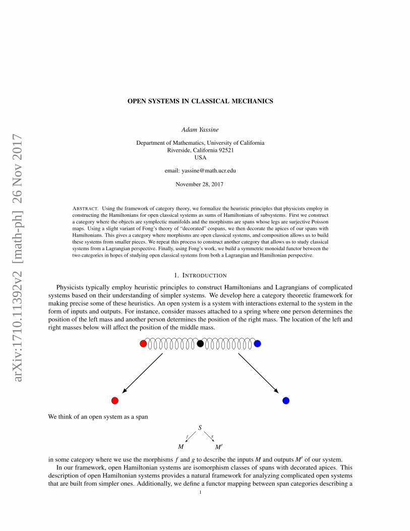
Physicists typically employ heuristic principles to construct Hamiltonians and Lagrangians of complicatedsystems based on their understanding of simpler systems. We develop here a category theoretic framework formaking precise some of these heuristics. An open system is a system with interactions external to the system in theform of inputs and outputs. For instance, consider masses attached to a spring where one person determines theposition of the left mass and another person determines the position of the right mass. The location of the left andright masses below will affect the position of the middle mass.

We think of an open system as a span

M M′

Sgf

in some category where we use the morphisms f and g to describe the inputs M and outputs M′ of our system.In our framework, open Hamiltonian systems are isomorphism classes of spans with decorated apices. This

description of open Hamiltonian systems provides a natural framework for analyzing complicated open systemsthat are built from simpler ones. Additionally, we define a functor mapping between span categories describing a

1

arX

iv:1

710.

1139

2v2

[m

ath-

ph]

26

Nov

201

7

2 OPEN SYSTEMS IN CLASSICAL MECHANICS

restricted class of Lagrangians and a span category describing Hamiltonians. This allows us to translate between theLagrangian and Hamiltonian descriptions of an open physical system.

In Section 3 we define and use a pullback to compose open systems. Since, pullbacks are not always objectsin our category. For instance, the category whose objects are differentiable manifolds and morphisms are smoothmaps, which we call Diff, has morphisms that are not ‘pullbackable’.This motivates us to look at a subcategory SurjSub of Diff whose objects are differentiable manifolds and morphismsare surjective submersions. SurjSub will have pullbacks over Diff. In Section 4 we define a span and using thefact that SurjSub is pullbackable over Diff allows us to build a category Span(SurjSub,Diff) whose objects aredifferentiable manifolds and morphisms are isomorphism classes of spans in SurjSub and composition is doneusing pullbacks in Diff. We wish to use diagrams of spans and compose spans in order to build larger systems. InSection 5 we define the category Symp whose objects are symplectic manifolds and morphisms are Poisson maps.We repeat the same construction as in the Section 4 with a subcategory SympSurj whose objects are symplecticmanifolds and morphisms are surjective Poisson maps. However, now the objects of our spans are drawn from Symp.This will lend itself to the description of Hamiltonian systems. Similar to Diff, the category Symp has morphismsthat are not pullbackable so we require a subcategory that has pullbacks over Symp. Thus, using the same ideas asin Section 4, we build a span category Span(SympSurj,Symp) whose objects are symplectic manifolds morphismsare isomorphism classes of spans in SympSurj and composition is done using pullbacks in Symp.

In Section 6, we apply Fong’s work approach to open systems to Hamiltonian mechanics. We use a variation ofFong’s theory of decorated cospans done in [8] to construct a category where a morphism is a diagram of the form:

M M′

S

RH

gf

In order to do this, we look at the category Symp whose objects are symplectic manifolds and morphisms arePoisson maps and its subcategory SympSurj whose objects are symplectic manifolds and morphisms are surjectivePoisson maps. As a result, we use this theory to build a category HamSy whose objects are symplectic manifoldsand a morphism from M to M′ is an isomorphism class spans where the legs are surjective Poisson maps, whoseapices are decorated by a smooth function called the Hamiltonian. The construction of HamSy builds the frameworkin modelling open systems using diagrams of spans. This motivates many examples in classical mechanics as wecan use category theory to formalize principles that physicists employ. Then in Section 7 we again use Fong’s workto construct another category, LagSy, whose morphisms are open systems in Lagrangian mechanics.

In general, we can use a Legendre transformation to go from the Lagrangian to the Hamiltonian. Using Fong’stheorem in [8] this gives rise to a functor from LagSy to HamSy by converting a restricted class of Lagrangiansinto Hamiltonians.

2. GEOMETRY BACKGROUND

We assume the reader is acquainted in basic objects of symplectic and Poisson geometry. However, we include abrief review of some of the ideas for the reader’s convenience.

Definition 1. Let f : K→M be a smooth map of manifolds, if the smooth linear map

d fp : TpK→ Tf (p)M

is surjective for all points p ∈ K, then we say that the function d fp is a submersion.

Definition 2. Let f : K→M be a smooth map of manifolds K and M. A point p ∈ K is called a regular point of f if


is surjective. A point c ∈M is called a regular value of f if every level set f−1(c) is a regular point.

OPEN SYSTEMS IN CLASSICAL MECHANICS 3

Definition 3. Let f : K→M be a smooth map of manifolds, if the smooth linear map


is surjective for all points p ∈ K, then we say that the function d fp is a submersion.

Definition 4. Let K,L⊂M be regular submanifolds such that every point p ∈ K∩L satisfies

TpK +TpL = TpM.

Then K,L are transverse manifolds.

Definition 5. A 1-form ω, on any manifold M is a map from the set of vector fields on M called Vect(M) to C∞(M)that is linear over C∞(M). In other words, for any u,v ∈ Vect(M) and g ∈C∞(M)

(1)ω(u+ v) = ω(u)+ω(v)

(2)ω(gv) = gω(v)

The space of all 1−forms on a manifold M will be denoted by Ω1(M) [2].

Example 1. We call the 1−form d f the differential of f or the exterior derivative of f where(1)

d f (u+ v) = d f (u)+d f (v)

(2)d f (gv) = gd f (v)

[2].

Definition 6. We define the smooth bijective map

[ : TpM→ T ∗p M

called flat map wherev 7→ ω(v, ·)

and] : T ∗p M→ TpM

to be called sharp map whereω(v, ·) 7→ v.

Note that this shows that these maps are isomorphisms.

Definition 7. The exterior algebra over a vector space V denoted ΛV is the algebra generated by V with therelation

v∧u =−u∧ v

for vectors u,v ∈V where ∧ is known as the wedge product [2].

We can extend the above definition to the concept of a manifold M by letting Ω1(M) play the role of V to get thefollowing definiton.


Definition 8. We define the differential forms on M, denoted Ω(M), to be the algebra generated by Ω1(M) withthe relations

ω ∧µ =−µ ∧ω

for all ω,µ ∈Ω1(M). Elements that are linear combinations of products of k 1−forms are called k−forms and thespace is denoted by Ωk(M). Moreover,

Ω(M) =⊕kΩk(M)

[2].

Definition 9. In particular when k = 2 ω is a 2−form. If

dω = 0,

then we say that ω is a closed 2−form. We say that ω is a nondegenerate 2−form if for any nonzero v there existsu such that

ω(v,u) 6= 0where u,v ∈ TxM [1].

Proposition 10. Given f ,g ∈C∞(M) and v f ∈ Vect(M) which is the smooth vector field associated to f , then

f ,g= v f (g) = dg(v f ).

Proof. We should note that given d f ∈Ω1(M) we have (d f )p ∈ T ∗p M. So given

(v f )p = ](d f )p ∈ TpM.

Since [ is an isomorphism, given d f theres exists a unique vector field v f such that

d f = ω(v f , ·).Hence,

d f (Z) = ω(v f ,z)for any z ∈ Vect(M). So in particular,

f ,g= v f (g) = dg(v f ).

Definition 11. Given functions f ,g,h ∈ C∞(M) and a,b ∈ R, a Poisson bracket on a manifold M is a binaryoperation

C∞(M)×C∞(M)→C∞(M),

( f ,g) 7→ f ,g,that satisfies the following:

(1) Antisymmetry f ,g=−g, f

(2) Bilinearity f ,ag+bh= a f ,g+b f ,h

(3) Jacobi Identity f ,g,h+g,h, f+h, f ,g= 0.

(4) Leibniz Law f g,h= f ,hg+ fg,h


[6].

Definition 12. A Poisson algebra is a commutative associative algebra ( f ,g) with Poisson bracket f ,g such thatthe four properties from above hold.

Proposition 13. The following bracket:

f ,g=n

∑i=1

∂ f∂qi

∂g∂ pi− ∂ f

∂ pi

∂g∂qi

is a Poisson algebra.

Proof. By Proposition 10, antisymmetry and bilinearity follow immediately so we now shift our attention to theJacobi Identity. Using the definition of

f ,g=n

∑i=1

∂ f∂qi

∂g∂ pi− ∂ f

∂ pi

∂g∂qi

we can write out each component of the Jacobi identity and see that each term ends up cancelling out in order togive us zero in the end.

f ,g,h=n

∑i=1

∂ f∂qi

∂g,h∂ pi

− ∂g,h∂ pi

∂g∂qi

=n

∑i=1

∂ f∂qi

∂

∂ pi

(n

∑j=1

∂g∂q j

∂h∂ p j− ∂h

∂q j

∂g∂ p j

)− ∂ f

∂ pi

∂

∂qi

(n

∑j=1

∂g∂q j

∂h∂ p j− ∂h

∂q j

∂g∂ p j

)

As a result, the above will produce eight terms when we apply the Leibniz law. Similarly,

g,h, f=n

∑i=1

∂g∂qi

∂h, f∂ pi

− ∂h, f∂ pi

∂g∂qi

will produce eight more terms and finally,

h, f ,g=n

∑i=1

∂h∂qi

∂ f ,g∂ pi

− ∂ f ,g∂ pi

∂H∂qi

will produce eight more terms, which in total gives us twenty four terms when we repeatedly apply the Leibniz law.However, since these are smooth vector fields by Clairout’s Theorem, the mixed partial terms will commute. Henceby adding up all twenty four terms, we indeed get zero, which proves the Poisson bracket is a Poisson algebra.

Definition 14. A Poisson manifold is a manifold M such that C∞(M) with ordinary multiplication of functions, andsome ·, · is a Poisson algebra.

Definition 15. Let (M,·, ·) be a Poisson manifold. Then for f ,g ∈C∞(M), by the Leibniz law we can define

f ,g= Π(d f ,dg)

where Π is a field of skew-symmetric bilinear forms on T ∗M. We say that

Π ∈ Γ((T ∗M∧T ∗M)∗) = Γ(T M∧T M) = Γ(Λ2T M)

is a bivector field [5].

Definition 16. The sections of ΛkT M are called k-vector fields or multivector fields for unspecified k on M. Thespace is denoted as Γ(ΛkT M) [5].

Definition 17. An almost Poisson structure ·, ·Π on a manifold M is called a Poisson structure if it satisfies theJacobi identity. Thus, a Poisson manifold (M,·, ·) is equipped with a Poisson structure ·, · and the correspondingbivector field Π is then called a Poisson tensor [5].


Definition 18. A Poisson manifold of even dimension M equipped with a closed nondegenerate 2−form ω satisfying f ,g= ω(v f ,vg) where v f is the vector field with v f (h) = h, f is a symplectic manifold.

Example 2. Let R2n have standard coordinates (x1, ...xn,y1, ...yn), the 2−form

ω =n

∑i=1

dxi∧dyi

is closed and nondegenerate.

Definition 19. Let (M,·, ·M) and (N,·, ·N) be Poisson manifolds. We say that a map

Φ : M→ N

is a Poisson map if, for any f ,g ∈C∞(N)

f ,gN Φ = f Φ,gΦM .

Let’s take a brief look at a fundamental Poisson map.Consider

(R4,·, ·R4

)and

(R2,·, ·R2

), where we use canonical coordinates (p1,q1, p2,q2) and (p1,q1) respec-

tively. The associated Poisson brackets are defined by the bivectors

Π =∂

∂ p1∧ ∂

∂q1+

∂

∂ p2∧ ∂

∂q2,

Π′ =

∂

∂ p1∧ ∂

∂q1.

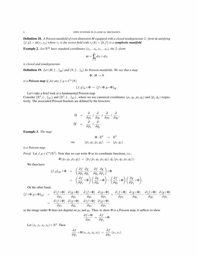
Example 3. The map

Φ : R4 → R2

via (p1,q1, p2,q2) 7→ (p1,q1)

is a Poisson map.

Proof. Let f ,g ∈C∞(R2). Note that we can write Φ as its coordinate functions, i.e.,

Φ(p1,q1, p2,q2) = (p1 (p1,q1, p2,q2) ,q1 (p1,q1, p2,q2)) .

We then have

f ,gR2 Φ =

(∂ f∂ p1

∂g∂q1− ∂ f

∂q1

∂g∂ p1

)Φ

=

(∂ f∂ p1Φ

)(∂g∂q1Φ

)−(

∂ f∂q1Φ

)(∂g∂ p1Φ

).

On the other hand,

f Φ,gΦR4 =∂ ( f Φ)

∂ p1· ∂ (gΦ)

∂q1− ∂ ( f Φ)

∂q1· ∂ (gΦ)

∂ p1+

∂ ( f Φ)

∂ p2· ∂ (gΦ)

∂q2− ∂ ( f Φ)

∂q2· ∂ (gΦ)

∂ p2

=∂ ( f Φ)

∂ p1· ∂ (gΦ)

∂q1− ∂ ( f Φ)

∂q1· ∂ (gΦ)

∂ p1,

as the image under Φ does not depend on p2 and q2. Thus, to show Φ is a Poisson map, it suffices to show

∂ f Φ

∂ p1=

∂ f∂ p1Φ.

Let (x1,y1,x2,y2) ∈ R4. Then

∂ f∂ p1Φ(x1,y1,x2,y2) =

∂ f∂ p1

(x1,y1) .


But∂ ( f Φ)

∂ p1(x1,y1,x2,y2) =

∂ f∂Φi

∣∣∣∣Φ(x1,y1,x2,y2)

· ∂Φi

∂ p1

∣∣∣∣(x1,y1,x2,y2)

=∂ f∂ p1

∣∣∣∣(x1,y1)

· ∂ p1

∂ p1

∣∣∣∣(x1,y1,x2,y2)

=∂ f∂ p1

(x1,y1) ,

for i = 1,2. In addition, p1 does not depend on p2,q1,q2 and q1 does not depend on p1, p2,q2. Hence,

f ,gR2 Φ = f Φ,gΦR4 ,

and Φ is a Poisson map.

Another property of Poisson maps is the following.

Proposition 20. Let X be a Poisson manifold and Y be a symplectic manifold. Any Poisson map

Φ : X → Y

is a submersion.

Proof. Suppose otherwise. Then the pushforward of Φ, dΦ(TxX) is a proper subspace V of TΦ(x)Y and dΦ(ΠX )⊆V ∧V. However, this is a contradiction to Φ being a Poisson map, which gives us the fact that the image of ΠXunder dΦ is symplectic [5].

Example 4. Suppose X and Y are symplectic manifolds. Then the projection map π : X×Y → X is a Poisson mapand a submersion.

3. PULLBACKS

In this section, we discuss the connection between submersions and transversality of manifolds. Indeed, theirconnection leads to the construction of a pullback in the category of differentiable manifolds denoted as Diff.We then want to extend this idea and look at the category of smooth manifolds whose morphisms are surjectivesubmersions, which we call SurjSub. Thus, we show that SurjSub is a category that has pullbacks over Diff.

Lemma 21. If K,L ⊂ M are transverse regular submanifolds then K ∩L is also a regular submanifold and itsdimension is

dimK +dimL−dimM,

where dimM = m, dimK = k, and dimL = l.

Proof. Let p ∈ K ∩L, then we can find a open neigborhood U of p where K ∩U = f−1(0) where 0 is a regularvalue for the function

f : K∩U → Rm−k

and L∩U = g−1(0) for a regular value 0 of a function

g : L∩U → Rm−l

by definition of regular manifolds. Then by definition of regular value, p must be a regular value for

( f ,g) : K∩L∩U → R2m−k−l

by definition of transversality and the above argument so then p will be a regular value in any neigborhood U of p.Hence,

( f ,g)|−1U (0,0) = f−1(0)∩g−1(0) = K∩L∩U

is a regular submanifold [9].

We can define transversality in terms of functions, which is the definition that is more frequently used.


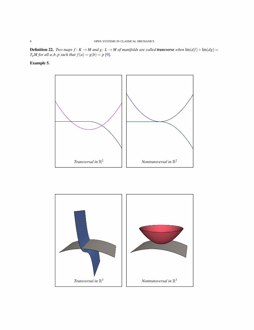
Definition 22. Two maps f : K→M and g : L→M of manifolds are called transverse when Im(d f )+ Im(dg) =TpM for all a,b, p such that f (a) = g(b) = p [9].

Example 5.

Nontransversal in R2Transversal in R2

Nontransversal in R3Transversal in R3


Definition 23. In any category C, given morphisms f : K→M and g : L→M, a pullback of f and g or fiberedproduct often denoted as K×M L consists of morphisms p,q such that f p = gq and the universal property holds.

That is given any object in our category, Q, which we call the competitor and morphisms p′ : Q→ K, q′ : Q→ Lsuch that f p′ = gq′ there exists a unique morphism ψ : Q→ K×M L with p′ = pψ and q′ = qψ.

K

K×M L L

M

Q

q

p g

f

∃!ψ

p′

q′

We want to use pullbacks in order to build larger systems from smaller systems. We should note that somecategories do not have pullbacks. One such category is Diff whose objects are differentiable manifolds andmorphisms are smooth maps. We show this in the following example.

Example 6. Consider the following diagram.

R

X R

R

R

q

p g

f

∃!ψ

p′

q′

Let g : R→ R be defined byg(y) = y2

and f : R→ R be defined byf (x) = x2.

Then if X is a pullback of the above diagram, it consists of morphisms p and q such that the diagram commutes. Bydefinition of the pullback, there exists a unique ψ : R→ X such that for any q′, p′ we have q′ = qψ and p′ = pψ,so in particular, let p′ = 1R and q′ =−1R. So suppose that X is a pullback in Diff. By Appendix 10, U : Diff→ Setpreserves pullbacks. As a result, U preserves limits. Thus,under the forgetful functor U, the image of X is a pullbackin Set and has the following underlying set

(x,y) ∈ R×R|y =±x.However, this underlying set has no smooth structure and hence is not an object in Diff.

In our example, since f and g were the function x2 this was the cause of the failure of the pullback not existingbecause f (x) = x2 is not transversal and is also is not a surjective submersion. We should note that if f or g is asurjective submersion, then transversality follows as we show in the next proposition.

Proposition 24. If f is a surjective submersion, then f and g are transverse.


Proof. If f is a surjective submersion then we know that d f is surjective. Then for any point p ∈M then for anytangent vector v ∈ TpM choose x ∈ f−1(p), which we can do by surjectivity. But since f is a submersion, then thereexists a tangent vector w ∈ Tf−1(p)K such that d f (w) = v. Therefore, Im(d f ) = TpM and hence

Im(d f )+ Im(dg) = TpM.

Theorem 25. If f : K→M, g : L→M are transverse smooth maps, then the fibered product

K×M L = (a,b) ∈ K×L : f (a) = g(b)

is a smooth manifold where the following diagram commutes. Note: ι is the inclusion map and h = f ∩g : (a,b) 7→f (a) = g(b).

K×M L

K×L

K

L

M

π1

π2

h

ι

g

f

ρ1

ρ2

Proof. Consider the graphs Γ f = (k,m)| f (k) = m,Γg = (l,m)|g(l) = m which are regular submanifolds ofK×M,L×M respectively. We show that the following intersection of regular submanifolds is transverse.

Γh = (Γ f ×Γg)∩ (K×L×∆M)

where∆M = (p, p) ∈M×M|p ∈M

is called the diagonal of M. So let f (k) = g(l) = p so that x = (k, l : p, p) ∈ K×M L and we see that by definition ofthe tangent space,

Tx(Γ f ×Γg) = ((v,d f (v)),(w,dg(w)))|v ∈ TkK, w ∈ TlL (∗)and

Tx(K×L×∆M) = ((v,m),(w,m))|v ∈ TkK, w ∈ TlL m ∈ TpM. (∗∗)But since f ,g are transversal then for any tangent vector m j ∈ TpM can be expressed as

d f (v j)+dg(w j)

for some (v j,w j) for j = 1,2. Thus, we can decompose a general tangent vector and using the linearity of thedifferential operator to M×M as

(m1,m2) = (d f (v2),d f (v2))+(dg(w1),dg(w1))+(d f (v1− v2),dg(w2−w1))

= (d f (v1)+dg(w1),d f (v2)+dg(w2)).

Hence this shows that (∗) and (∗∗) are transverse. So then by Lemma 21, we get that Γh is a regular submanifold ofK×L×M×M. But it actually is a regular submanifold in K×L×∆M because we can compose with the projectionmap and hence it can be seen as a regular submanifold in K×L×∆M. Then taking the restriction of the projectionmap onto K×L to the submanifold Γh is a smooth embedding whose image is exactly K×M L. Hence, K×M L isa regular submanifold where Γh can be viewed as the graph of a smooth map h : K×M L→M, which makes thediagram commute [9].

The next proposition that we state will be used to show that our maps are submersions in the next corollary.


Proposition 26. If α ∈ K×M L, then Tα(K×M L)∼= TkK×TmM TlL, where

TkK×TmM TlL = (u,w) ∈ TkK×TlL|d f (u) = dg(w).

Corollary 27. Surjective submersions are pullbackable: for any surjective submersion g : L→M and any smoothmap f : K→M, then the pullback exists:

K×M L

Q

K

L

M

π1

π2

∃!ψ

g

f

ρ1

ρ2

K×M L is a pullback in the category of smooth manifolds, Diff whose objects are smooth manifolds and morphismsare smooth maps. Furthermore, π1 is a surjective submersion.

Proof. By definition of the competitor, we have the morphisms ρ1,ρ2 such that

gρ2 = f ρ1.

Define

ψ : Q→ K×M L

by

ψ(x) = (ρ1(x),ρ2(x)).

To show ψ is well defined, suppose

ψ(x) 6= ψ(x′).

Then,

(ρ1(x),ρ2(x)) 6= (ρ1(x′),ρ2(x′)).

So without loss of generality, if ρ1(x) 6= ρ1(x′) then x 6= x′ since ρ1 is a well defined morphism. So we see that

π2 ψ(x) = π2(ρ1(x),ρ2(x)) = ρ2(x).

Hence, π2 ψ = ρ2 for all x ∈ Q. Similarly,

π1 ψ = ρ1.

Then

gπ2 ψ(x) = gρ2(x)

and

f π1 ψ(x) = f ρ1(x).

But since f ρ1 = gρ2, then

gπ2 ψ = f π1 ψ.

Therefore, ψ is a well defined morphism. Since K×M L is a fibered product, then by the universal property ofproducts, ψ will be unique. We now turn our attention to showing that π1 is a surjective submersion.


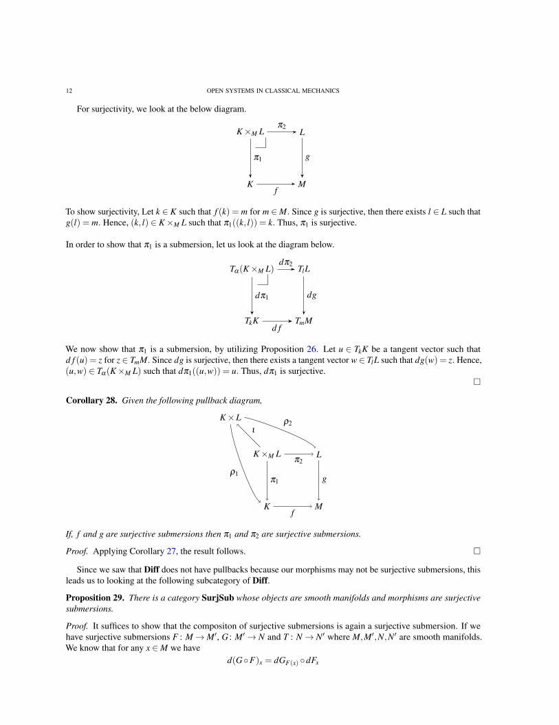
For surjectivity, we look at the below diagram.

K

K×M L L

M

π2

π1 g

f

To show surjectivity, Let k ∈ K such that f (k) = m for m ∈M. Since g is surjective, then there exists l ∈ L such thatg(l) = m. Hence, (k, l) ∈ K×M L such that π1((k, l)) = k. Thus, π1 is surjective.

In order to show that π1 is a submersion, let us look at the diagram below.

TkK

Tα(K×M L) TlL

TmM

dπ2

dπ1 dg

d f

We now show that π1 is a submersion, by utilizing Proposition 26. Let u ∈ TkK be a tangent vector such thatd f (u) = z for z ∈ TmM. Since dg is surjective, then there exists a tangent vector w ∈ TlL such that dg(w) = z. Hence,(u,w) ∈ Tα(K×M L) such that dπ1((u,w)) = u. Thus, dπ1 is surjective.

Corollary 28. Given the following pullback diagram,

K×M L

K×L

K

L

M

π1

π2

ι

g

f

ρ1

ρ2

If, f and g are surjective submersions then π1 and π2 are surjective submersions.

Proof. Applying Corollary 27, the result follows.

Since we saw that Diff does not have pullbacks because our morphisms may not be surjective submersions, thisleads us to looking at the following subcategory of Diff.

Proposition 29. There is a category SurjSub whose objects are smooth manifolds and morphisms are surjectivesubmersions.

Proof. It suffices to show that the compositon of surjective submersions is again a surjective submersion. If wehave surjective submersions F : M→M′, G : M′→ N and T : N→ N′ where M,M′,N,N′ are smooth manifolds.We know that for any x ∈M we have

d(GF)x = dGF(x) dFx


by the Chain Rule. But because F and G are submersions, we know that dG and dF are surjective and because thecomposition of surjective maps is surjective; moreover, the composition of smooth maps is smooth. Since we haveshown that the composition of smooth submersions is a smooth submersion, then

d((T G)F)x = d(T G)F(x) dFx = dTGF(x) dGFx dFx.

This is a smooth submersion and doing a similar computation we get

d((T G)F)x = d(T (GF))x.

Hence, associativity holds. For the right unit law we have

d(F 1x)x = dFx d1x = dFx 1TxM = dFx.

Similarly, the left unit law will also hold. Hence, SurjSub is a category.

4. SPANS

In this section, we remind the reader that D is a category with pullbacks over C. We can define the categorySpan(C, D) where objects are in C and morphisms are isomorphism classes of spans in D and composition isdone using pullbacks in C. The example that we should keep in mind is the category of smooth manifolds whosemorphisms are surjective submersions, which we will call SurjSub. In 1967 J. Benabou [3] proved significantresults by introducing bicategories. We then show that there is a category whose objects are smooth manifolds andwhose morphisms are isomorphism classes of spans whose legs are surjective submersions.

Definition 30. A span from M to M′ in a category C is an object S in C with a pair of morphisms f : S→M andg : S→M′. M and M′ are known as feet and S is known as the apex of the span.

M M′

Sgf

Definition 31. A map of spans is a morphism j : S→ S′ in a category C between apices of two spans MSM′ and MS′M′such that both the following triangles commute. In particular, when j is an isomorphism, we have an isomorphismof spans.

M M′

S

S′

gf

g′f ′∼= j

Given spans MSM′ and MS′M′ , the isomorphism class of spans is the class of spans S such that there exists anisomorphism between apices j : S→ S′ such that the two side by side triangles commute.

M M′

S

S′

gf

g′f ′j

Definition 32. An isomorphism class of spans is an equivalence class of spans where the equivalence relation isisomorphism.

Definition 33. Composition of spans is given by pullback over a shared foot.


We should note that pullbacks are unique only up to isomorphism, which is why we need to take isomorphismclasses of spans to obtain a category. For instance, SurjSub does not have pullbacks, which we show in the nextexample. As a result, we need to specify where we pullback when composing spans.

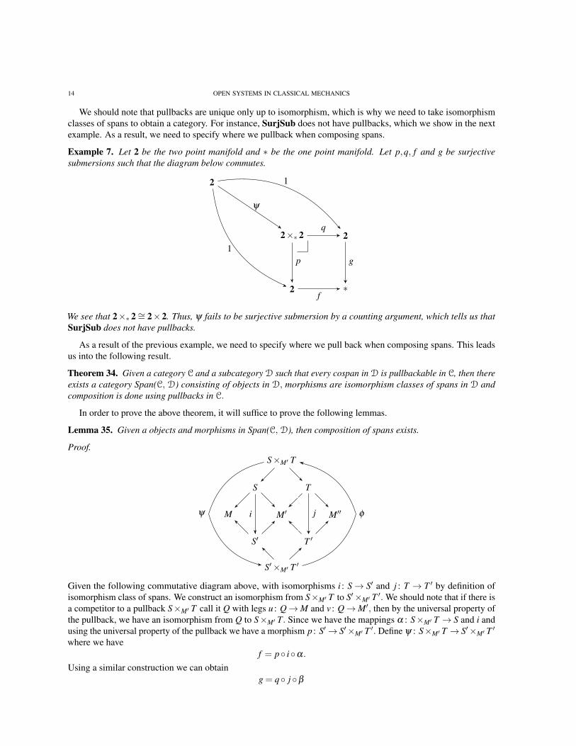
Example 7. Let 2 be the two point manifold and ∗ be the one point manifold. Let p,q, f and g be surjectivesubmersions such that the diagram below commutes.

2

2×∗ 2 2

∗

2

q

p g

f

ψ

1

1

We see that 2×∗ 2∼= 2×2. Thus, ψ fails to be surjective submersion by a counting argument, which tells us thatSurjSub does not have pullbacks.

As a result of the previous example, we need to specify where we pull back when composing spans. This leadsus into the following result.

Theorem 34. Given a category C and a subcategory D such that every cospan in D is pullbackable in C, then thereexists a category Span(C, D) consisting of objects in D, morphisms are isomorphism classes of spans in D andcomposition is done using pullbacks in C.

In order to prove the above theorem, it will suffice to prove the following lemmas.

Lemma 35. Given a objects and morphisms in Span(C, D), then composition of spans exists.

Proof.

M M′ M′′

S

S′

T

T ′

S×M′ T

S′×M′ T ′

ψ φi j

Given the following commutative diagram above, with isomorphisms i : S→ S′ and j : T → T ′ by definition ofisomorphism class of spans. We construct an isomorphism from S×M′ T to S′×M′ T ′. We should note that if there isa competitor to a pullback S×M′ T call it Q with legs u : Q→M and v : Q→M′, then by the universal property ofthe pullback, we have an isomorphism from Q to S×M′ T. Since we have the mappings α : S×M′ T → S and i andusing the universal property of the pullback we have a morphism p : S′→ S′×M′ T ′. Define ψ : S×M′ T → S′×M′ T ′

where we havef = p iα.

Using a similar construction we can obtaing = q j β


where q : T ′→ S′×M′ T ′ exists by the universal property of the pullback and β : S×M′ T → T. Hence, we can define

ψ = f ×g.

Similarly, we can construct a map φ : S′×M′ T ′→ S×M′ T. Using the fact that S′×M′ T ′ is a pullback, we havemorphisms α ′ : S′×M′ T ′→ S′ and β ′ : S′×M′ T ′→ T ′. Then define

φ = f ′×g′

where f ′ = p′ i−1 α ′ and g′ = q′ j−1 β ′. In addition, p′ : S→ S×M′ T and q′ : T → S×M′ T. Therefore, byconstruction we see that

ψ φ = 1S×M′T

andφ ψ = 1S′×M′T

′

and hence, we have an isomorphism between S×M′ T and S′×M′ T ′ which completes the proof.

Lemma 36. Given objects and morphisms in Span(C, D) then associativity law holds.

Proof.

M M′ M′′ M′′′

S

S′

T

T ′

U

U ′

S×M′ T

T ′×M′′U ′

(S×M′ T )×M′′U

S×M′ (T ×M′′U)

i j k

By our hypothesis, S×M′ T is a pullback to the diagram of spans MSM′ and M′TM′′ as well as (S×M′ T )×M′′U isa pullback to the diagram of spans SS×M′ TT and M′′UM′′′ . Then by definition, (S×M′ T )×M′′U is a pullback andhence a limit making the diagram commute. Similarly, S×M′ (T ×M′′U) is a limit to the same diagram and hence,by the universal property of pullbacks, (S×M′ T )×M′′U will be isomorphic to S×M′ (T ×M′′U).

Lemma 37. Given objects and morphisms in Span(C, D), then left and right unit laws hold.

Proof.

M M′ M′

S M′

S×M′ M′

S

f 1M′

ψφ


M′

M′

S×M′ M′

S

S

f

1M′ f

1S

∃!ψ

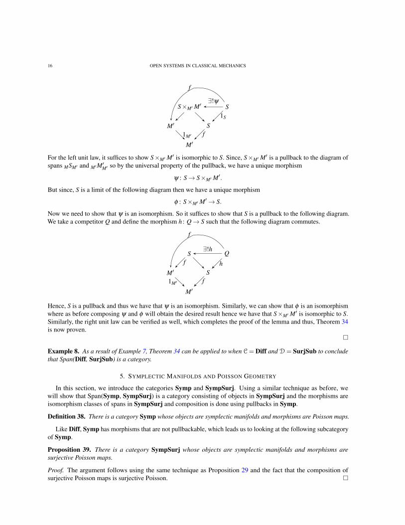
For the left unit law, it suffices to show S×M′ M′ is isomorphic to S. Since, S×M′ M′ is a pullback to the diagram ofspans MSM′ and M′M′M′ so by the universal property of the pullback, we have a unique morphism

ψ : S→ S×M′ M′.

But since, S is a limit of the following diagram then we have a unique morphism

φ : S×M′ M′→ S.

Now we need to show that ψ is an isomorphism. So it suffices to show that S is a pullback to the following diagram.We take a competitor Q and define the morphism h : Q→ S such that the following diagram commutes.

M′

M′

S

S

Q

f

1M′ f

f h

∃!h

Hence, S is a pullback and thus we have that ψ is an isomorphism. Similarly, we can show that φ is an isomorphismwhere as before composing ψ and φ will obtain the desired result hence we have that S×M′ M′ is isomorphic to S.Similarly, the right unit law can be verified as well, which completes the proof of the lemma and thus, Theorem 34is now proven.

Example 8. As a result of Example 7, Theorem 34 can be applied to when C= Diff and D= SurjSub to concludethat Span(Diff, SurjSub) is a category.

5. SYMPLECTIC MANIFOLDS AND POISSON GEOMETRY

In this section, we introduce the categories Symp and SympSurj. Using a similar technique as before, wewill show that Span(Symp, SympSurj) is a category consisting of objects in SympSurj and the morphisms areisomorphism classes of spans in SympSurj and composition is done using pullbacks in Symp.

Definition 38. There is a category Symp whose objects are symplectic manifolds and morphisms are Poisson maps.

Like Diff, Symp has morphisms that are not pullbackable, which leads us to looking at the following subcategoryof Symp.

Proposition 39. There is a category SympSurj whose objects are symplectic manifolds and morphisms aresurjective Poisson maps.

Proof. The argument follows using the same technique as Proposition 29 and the fact that the composition ofsurjective Poisson maps is surjective Poisson.


We now turn our attention to an important result in symplectic geometry known as Darboux’s Theorem. Darboux’sTheorem allows us to locally express symplectic 2−forms in terms of local coordinates, which we use to proveTheorem 42.

Theorem 40 (Darboux). For every symplectic manifold (M,ω) of dimension 2n we have that for any x ∈M, thereexists a local coordinate system (q1, ...,qn, p1, ..., pn) called Darboux coordinates in a neighborhood U of x suchthat

ω =n

∑i=1

dqi∧d pi.

In Theorem 25, we showed that surjective submersions were pullbackable over Diff. Our goal is to show thatsurjective Poisson maps are pullbackable over Symp. We use Darboux’s theorem to show that the product ofsymplectic manifolds is symplectic. This approach is used because we will use the Darboux coordinates along theproduct of symplectic manifolds in order to construct the symplectic 2−form along the pullback.

Lemma 41. Let (X ,ωX ),(Y,ωY ) be symplectic manifolds. Let ρX : X×Y → X and ρY : X×Y →Y be the standardprojection maps. Then (X×Y,ω) is a symplectic manifold with

ω = ρ∗X ωX +ρ

∗Y ωY .

Proof. Let X and Y be symplectic manifolds of dimension 2m and 2n respectively. Since X and Y are smoothmanifolds, X×Y is a smooth manifold of dimension 2m+2n. To show that the even dimensional manifold X×Y issymplectic, it suffices to show that the 2−form ω given in the statement of the lemma is closed and nondegenerate.The commutativity of d with ρ∗X and ρ∗Y together with the closedness of ωX and ωY imply that

dω = d(ρ∗X ωX +ρ∗Y ωY ) = d(ρ∗X ωX )+d(ρ∗Y ωY ) = ρ

∗X dωX +ρ

∗Y dωY = 0.

Thus, ω is a closed 2−form.Since X is symplectic, Darboux’s theorem implies that for any x in X there exists an open neighborhood U of x

and local coordinates (xi, pi)mi=1 on U such that

ωX =m

∑i=1

dxi∧d pi.

Similarly, for any y in Y there exists an open neighborhood V of y and local coordinates (yi,qi)nj=1 on V such that

ωY =n

∑j=1

dy j ∧dq j.

Let (x1, ...xm, p1, ...pm, y1, ...yn, q1, ...qn) be local coordinates on U×V in X×Y with

xi = xi ρX , pi = pi ρX , y j = y j ρY and qj = qj ρY.

Thus,ρ∗X (dxi) = d(xi ρX ) = dxi.

The other coordinates follow in a similar manner, and so ω can be written in local coordinates on U×V as

ω =m

∑i=1

dxi∧d pi +n

∑j=1

dy j ∧dq j.

For ω to be nondegenerate means that for any α in X ×Y and any nonzero v in Tα(X ×Y ) there exists u inTα(X ×Y ) such that ω(v,u) is nonzero. Suppose v in Tα(X ×Y ) and for any u in Tα(X ×Y ), ω(v,u) is 0. Thereexists coefficients ai,bi,c j,e j such that v = ai∂ xi +bi∂ pi + c j∂ y j + e j∂ q j. If u = ∂ xi then

ω(v,u) = ω(ai∂ xi +bi

∂ pi + c j∂ y j + e j

∂ q j,∂ xi) =−bi = 0.

Thus, bi = 0. By assumption, ω(v,∂ xi) = ω(v,∂ pi) = ω(v,∂ y j) = ω(v,∂ q j) = 0. Following the above calculation,we have that

ai = c j = e j = 0, hence, v = 0.By contraposition, ω is nondegenerate.


We are now ready to state the theorem, which will help us show that SympSurj has pullbacks over Symp. Theproof of this theorem requires a lemma, which we will state and prove after proving the theorem.

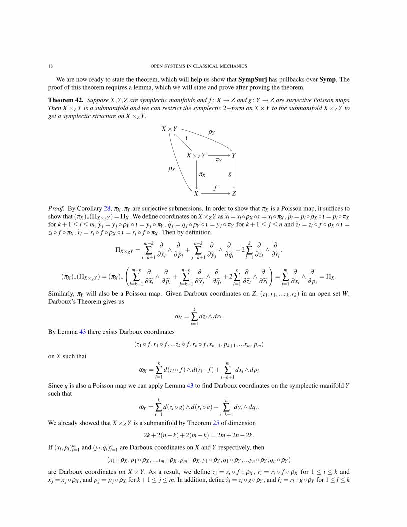
Theorem 42. Suppose X ,Y,Z are symplectic manifolds and f : X → Z and g : Y → Z are surjective Poisson maps.Then X×Z Y is a submanifold and we can restrict the symplectic 2−form on X×Y to the submanifold X×Z Y toget a symplectic structure on X×Z Y .

X×Z Y

X×Y

X

Y

Z

πX

πY

ι

g

f

ρX

ρY

Proof. By Corollary 28, πX ,πY are surjective submersions. In order to show that πX is a Poisson map, it suffices toshow that (πX )∗(ΠX×ZY )=ΠX . We define coordinates on X×Z Y as xi = xiρX ι = xiπX , pi = piρX ι = piπXfor k+1 ≤ i ≤ m, y j = y j ρY ι = y j πY , q j = q j ρY ι = y j πY for k+1 ≤ j ≤ n and zl = zl f ρX ι =zl f πX , rl = rl f ρX ι = rl f πX . Then by definition,

ΠX×ZY =m−k

∑i=k+1

∂

∂ xi∧ ∂

∂ pi+

n−k

∑j=k+1

∂

∂ y j∧ ∂

∂ qi+2

k

∑l=1

∂

∂ zl∧ ∂

∂ rl.

(πX )∗(ΠX×ZY ) = (πX )∗

(m−k

∑i=k+1

∂

∂ xi∧ ∂

∂ pi+

n−k

∑j=k+1

∂

∂ y j∧ ∂

∂ qi+2

k

∑l=1

∂

∂ zl∧ ∂

∂ rl

)=

m

∑i=1

∂

∂xi∧ ∂

∂ pi= ΠX .

Similarly, πY will also be a Poisson map. Given Darboux coordinates on Z, (z1,r1, ...zk,rk) in an open set W,Darboux’s Theorem gives us

ωZ =k

∑i=1

dzi∧dri.

By Lemma 43 there exists Darboux coordinates

(z1 f ,r1 f , ...zk f ,rk f ,xk+1, pk+1, ...xm, pm)

on X such that

ωX =k

∑i=1

d(zi f )∧d(ri f )+m

∑i=k+1

dxi∧d pi

Since g is also a Poisson map we can apply Lemma 43 to find Darboux coordinates on the symplectic manifold Ysuch that

ωY =k

∑i=1

d(zi g)∧d(ri g)+n

∑i=k+1

dyi∧dqi.

We already showed that X×Z Y is a submanifold by Theorem 25 of dimension

2k+2(n− k)+2(m− k) = 2m+2n−2k.

If (xi, pi)mi=1 and (yi,qi)

ni=1 are Darboux coordinates on X and Y respectively, then

(x1 ρX , p1 ρX , ...xm ρX , pm ρX ,y1 ρY ,q1 ρY , ...yn ρY ,qn ρY )

are Darboux coordinates on X ×Y. As a result, we define zi = zi f ρX , ri = ri f ρX for 1 ≤ i ≤ k andx j = x j ρX , and p j = p j ρX for k+1≤ j≤m. In addition, define zl = zl gρY , and rl = rl gρY for 1≤ l ≤ k


and yt = yt ρY , qi = qt ρY for k+1≤ t ≤ n. Hence, we can rewrite the coordinates as (zi, ri, x j, p j, zl , rl , yt , qt).Thus,

ω =k

∑i=1

dzi∧dri +m

∑j=k+1

dx j ∧d p j +k

∑l=1

dzl ∧drl +n

∑t=k+1

dyt ∧dqt .

Then by the definition of the pullback,

ωX×ZY =m−k

∑i=k+1

dxi∧d pi +n−k

∑j=k+1

dy j ∧dq j +2k

∑l=1

dzl ∧drl .

Since ω is closed, then ωX×ZY will be closed and nondegeneracy follows immediately, which completes the proof.

The following lemma is proven using a technique by A. Cannas da Silva and A. Weinstein in [5].

Lemma 43. Let X and Z be symplectic manifolds of dimensions 2m and 2k respectively. Suppose that f : X → Zis a Poisson map that is a surjective submersion. Given any z ∈ Z and a choice of Darboux coordinates (zi,ri)

ki=1

in a neighborhood U of z, and given any x ∈ X such that f (x) = z, there exists Darboux coordinates in someneighborhood V of x, (xi, pi)

mi=1, such that

xi = zi fand

pi = ri ffor 1≤ i≤ k.

Proof. Let p ∈U ⊆ X , where U is open. Since f is a surjective submersion, then f : U → f (U) is an open map.Further restrict U so that U is in a Darboux coordinate chart, as well as f (U). Let (v1, ...,v2k) be Hamiltonian vectorfields associated to the coordinate functions on f (U), such that

v1 =−∂

∂ r1, ...,vk =−

∂

∂ rk,vk+1 =

∂

∂ z1, ...,v2k =

∂

∂ zk.

Recall, thatΠ−1Z : T Z→ T ∗Z,

is an isomorphism and so Π−1Z (vi) is a covector. Thus, f ∗Π−1(vi) is a pullback covector. We define the horizontal

liftHp(vi) = ΠX ( f ∗Π−1

Z (vi)) ∈ TpX .

Now because f is a Poisson map, we get that

d f (Hp(vi)) = vi|p.As a result, H•(vi))i=1,...2k is a family of smooth vector fields that pointwise span a 2k dimensional subspace of TUor in other words, these are local sections that are linearly independent. If we set v1 =

∂

∂ z1,v2 =

∂

∂ r1, ...v2k =

∂

∂ rk

and ui = H(vi) we have that 〈ui〉2ki=1 is closed under the Lie bracket [·, ·]. So by the Frobenius theorem, there exists

Z ⊆U such that Z is a 2k submanifold and T Z is locally trivialized by 〈ui〉2ki=1. Now, we show that Z is symplectic.

Since f ∗ωZ is closed on X because the differential commutes with the pullback and ωZ is closed, then f ∗ωZ isclosed on Z. As a consequence of the rank-nullity theorem, TpX = TpZ⊕ker(d fp). To show nondegeneracy on Z,suppose there exists v ∈ TpZ such that for any u ∈ TpZ,

f ∗ωZ(v,u) = 0.

Then,ωZ | f (p)( f∗v, f∗u) = f ∗ωZ |p(v,u) = 0.

But for each u′ ∈ Tf (p)Z there exists u ∈ TpX such that f∗(u) = u′ because f is a submersion. Thus, for anyu′ ∈ Tf (p)Z,

ωZ | f (p)( f∗v,u′) = 0.


However, since ωZ is nondegenerate then f∗v = 0. Hence, this means that v ∈ ker(d fp), but because v ∈ TpZ andTpX = TpZ⊕ker(d fp), then v = 0. Therefore, f ∗ωZ is closed and nondegenerate on Z, which means that Z is a 2kdimensional symplectic submanifold of X . As a result,for any q ∈ Z there is a Darboux chart for X such that Z isgiven by the equations xi = 0, pi = 0 for i > 2k, which completes the proof.

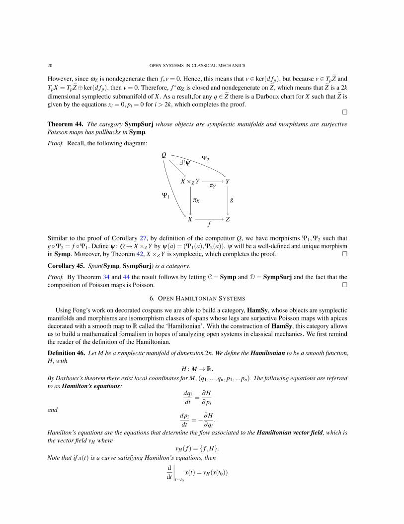
Theorem 44. The category SympSurj whose objects are symplectic manifolds and morphisms are surjectivePoisson maps has pullbacks in Symp.

Proof. Recall, the following diagram:

X×Z Y

Q

X

Y

Z

πX

πY

∃!ψ

g

f

Ψ1

Ψ2

Similar to the proof of Corollary 27, by definition of the competitor Q, we have morphisms Ψ1,Ψ2 such thatgΨ2 = f Ψ1. Define ψ : Q→ X×Z Y by ψ(a) = (Ψ1(a),Ψ2(a)). ψ will be a well-defined and unique morphismin Symp. Moreover, by Theorem 42, X×Z Y is symplectic, which completes the proof.

Corollary 45. Span(Symp, SympSurj) is a category.

Proof. By Theorem 34 and 44 the result follows by letting C = Symp and D = SympSurj and the fact that thecomposition of Poisson maps is Poisson.

6. OPEN HAMILTONIAN SYSTEMS

Using Fong’s work on decorated cospans we are able to build a category, HamSy, whose objects are symplecticmanifolds and morphisms are isomorphism classes of spans whose legs are surjective Poisson maps with apicesdecorated with a smooth map to R called the ‘Hamiltonian’. With the construction of HamSy, this category allowsus to build a mathematical formalism in hopes of analyzing open systems in classical mechanics. We first remindthe reader of the definition of the Hamiltonian.

Definition 46. Let M be a symplectic manifold of dimension 2n. We define the Hamiltonian to be a smooth function,H, with

H : M→ R.By Darboux’s theorem there exist local coordinates for M, (q1, ...,qn, p1, ...pn). The following equations are referredto as Hamilton’s equations:

dqi

dt=

∂H∂ pi

andd pi

dt=−∂H

∂qi.

Hamilton’s equations are the equations that determine the flow associated to the Hamiltonian vector field, which isthe vector field vH where

vH( f ) = f ,H.Note that if x(t) is a curve satisfying Hamilton’s equations, then

ddt

∣∣∣∣t=t0

x(t) = vH(x(t0)).


Furthermore, the properties of the Poisson bracket guarantee that

ω(vH , ·) = dH.

Theorem 47. There is a category HamSy where an object is a symplectic manifold M. A morphism from M to M′

is an isomorphism class of spans MSM′ where the legs are surjective Poisson maps, and the apex is decorated by asmooth map H : S→ R called the Hamiltonian. We compose morphisms as follows:

M M′ M′′

S S′

S×M′ S′

R

f g f ′ g′

πS′

H H ′H ′′

πS

We have smooth maps H πS : S×M′ S′→ R, H ′ πS′ : S×M′ S′→ R.So we define the Hamiltonian on the pullback as

H ′′ = H πS +H ′ πS′ .

Proof. In [8], Fong takes a category C with finite colimits and a symmetric lax monoidal functor (F,ϕ) : (C,+)→(Set,×) and defines decorated cospans. We should note that our work uses a lax symmetric monoidal functor

(F,ϕ) : (C,+)→ (Set,×).The coproduct + in C is also the product × in Cop, so (C,+)op = (Cop,×). In addition, if C has finite limits and

M M′ M′′

S S′

S×M′ S′

f g f ′ g′

πS′πS

is a pullback, then there exists a canonical morphism

[πS,π′S] : S×M′ S

′→ S×S′

where [πS,π′S] is the inclusion map.

Let C be a category with finite limits and let

(F,ϕ) : (C,×)op→ (Set,×)be a lax symmetric monoidal functor. Given objects M,M′ ∈ C an F-decorated span, from M to M′′ is a pairconsisting of a span MSM′ in C and an element d ∈ F(S). We call d the decoration. Given two decorated spans

(MSM′ ,d ∈ F(S)), (M′S′M′′ ,d

′ ∈ F(S′))

their composite is the span from M to M′ constructed via pullback:

M M′ M′′

S S′

S×M′ S′

f g f ′ g′

πS′πS


together with the decoration obtained by applying the map

F(S)×F(S′)ϕS,S′−−→ F(S×S′)

F([πS,πS′ ])−−−−−−→ F(S×M′ S′).

to the pair (d,d′) ∈ F(S)×F(S′). Here [πS,πS′ ] : S×S′→ S×M′ S′ is the morphism in (C,×)op.Fong then uses this idea to develop a decorated cospan category whose objects are in C and morphisms are

isomorphism classes of decorated cospans where composition is done using pushouts over C. We however, willadapt this idea and apply it to spans by working with the opposite categories. Furthermore, our categories will nothave finite limits. For us, SympSurj does not have morphisms that are pullbackable but instead has morphisms thatare pullbackable over Symp. We use this variation of Fong’s work by taking our decorations to be Hamiltonians.We have the following diagram of spans in the category SympSurj.

M M′ M′′

S S′

S×M′ S′

S×S′

πS′

ρS ρS′

ι

πS

We want to show that

(F,ϕ) : (SympSurj,×)op→ (Set,×)

is a lax symmetric monoidal functor where

ϕS,S′ : F(S)×F(S′)→ F(S×S′)

by

(HS,HS′) 7→ HS ρS +HS′ ρS′

and

ϕ : ∗→ F( /0)

where ∗ is the terminal object in Set and /0 is the unit for SympSurjop. We need to check the commutativity ofthe right unitor diagram:

F(S)

∗×F(S) F( /0)×F(S)

F( /0×S)

ϕ× id

∼= ϕ /0,S

∼=

So if we compose the following

(ϕ× id)(∗,HS) = (H/0,HS)

then applying

ϕ /0,S(H/0,HS) = H/0 ρ /0 +HS ρS = HS ∈ F( /0×S)∼= F(S).


We should note that by definition of the Hamiltonian, H∗ = 0. This shows the commutativity of the right unitor.The left unitor follows similarly. For the associator hexagon, consider the following diagram:

F(S× (S′×S′′))

F(S)×F(S′×S′′) F(S×S′)×F(S′′)

F((S×S′)×S′′)

F(S)× (F(S′)×F(S′′)) (F(S)×F(S′))×F(S′′)

ϕS,S′×S′′ ϕS×S′,S′′

∼=

∼=

id×ϕS′,S′′ ϕS′,S′′ × id

If we start from the upper left corner and proceeding downward,

(id×ϕS′,S′′)(HS,(HS′ ,HS′′)) = (HS,HS′ ρS′ +HS′′ ρS′′)

then applying

(ϕS,S′×S′′)(HS,HS′ ρS′ +HS′′ ρS′′) = HS ρS +(HS′ ρS′ +HS′′ ρS′′)ρS′×S′′

= HS ρS +(HS′ ρS′ +HS′′ ρS′′) ∈ F(S× (S′×S′′)).

Since F(S× (S′×S′′))∼= F((S×S′)×S′′) then HS ρS +(HS′ ρS′ +HS′′ ρS′′) has an isomorphic copy in F((S×S′)×S′′),

(HS ρS +HS′ ρS′)+HS′′ ρS′′ .

Now, if we start again from the upper corner and proceed to the right and downward, we start with (HS,(HS′ ,HS′′))∈F(S)× (F(S′)×F(S′′)) which has an isomorphic copy in (F(S)×F(S′))×F(S′′), ((HS,HS′),HS′′). Then applyingthe following we get

(ϕS,S′ × id)((HS,HS′),HS′′) = (HS ρS +HS′ ρS′ ,HS′′).

Then,

(ϕS×S′,S′′)(HS ρS +HS′ ρS′ ,HS′′) = (HS ρS +HS′ ρS′)ρS×S′ +HS′′ ρS′′ ∈ F((S×S′)×S′′).

But(HS ρS +HS′ ρS′)ρS×S′ +HS′′ ρS′′ = (HS ρS +HS′ ρS′)+HS′′ ρS′′ .

This shows the square commutes, which proves the hexagonal axiom and completes the proof.

With the construction of HamSy we can now use this new category to look at the following examples of opensystems in classical mechanics.

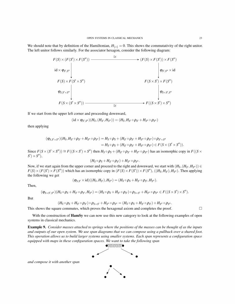
Example 9. Consider masses attached to springs where the positions of the masses can be thought of as the inputsand outputs of our open system. We use span diagrams that we can compose using a pullback over a shared foot.This operation allows us to build larger systems using smaller systems. Each span represents a configuration spaceequipped with maps in these configuration spaces. We want to take the following span

and compose it with another span


in order to build a composite span

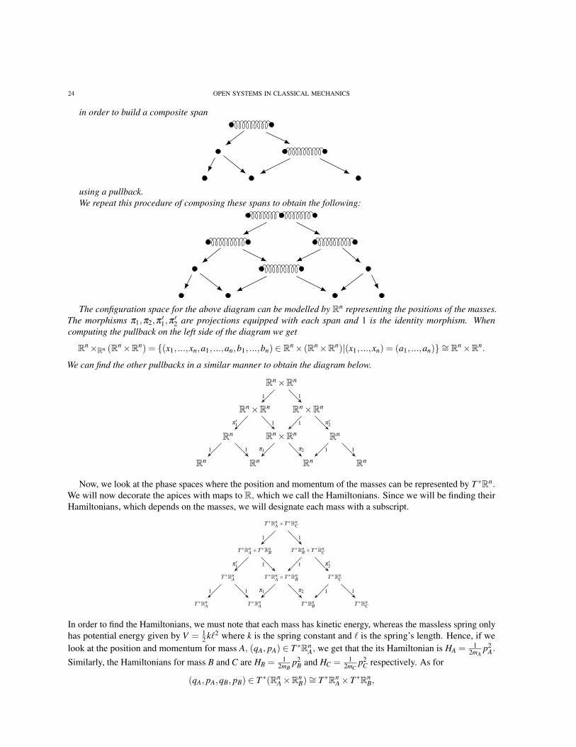
using a pullback.We repeat this procedure of composing these spans to obtain the following:

The configuration space for the above diagram can be modelled by Rn representing the positions of the masses.The morphisms π1,π2,π

′1,π′2 are projections equipped with each span and 1 is the identity morphism. When

computing the pullback on the left side of the diagram we get

Rn×Rn (Rn×Rn) = (x1, ...,xn,a1, ...,an,b1, ...,bn) ∈ Rn× (Rn×Rn)|(x1, ...,xn) = (a1, ...,an) ∼= Rn×Rn.

We can find the other pullbacks in a similar manner to obtain the diagram below.

Rn Rn Rn Rn

Rn Rn×Rn Rn

Rn×Rn Rn×Rn

Rn×Rn

1 1 π1 π2 11

π ′1 1 1 π ′2

1 1

Now, we look at the phase spaces where the position and momentum of the masses can be represented by T ∗Rn.We will now decorate the apices with maps to R, which we call the Hamiltonians. Since we will be finding theirHamiltonians, which depends on the masses, we will designate each mass with a subscript.

T ∗RnA T ∗Rn

A T ∗RnB T ∗Rn

C

T ∗RnA T ∗Rn

A×T ∗RnB T ∗Rn

C

T ∗RnA×T ∗Rn

B T ∗RnB×T ∗Rn

C

T ∗RnA×T ∗Rn

C

1 1 π1 π2 11

π ′1 1 1 π ′2

1 1

In order to find the Hamiltonians, we must note that each mass has kinetic energy, whereas the massless spring onlyhas potential energy given by V = 1

2 k`2 where k is the spring constant and ` is the spring’s length. Hence, if welook at the position and momentum for mass A, (qA, pA) ∈ T ∗Rn

A, we get that the its Hamiltonian is HA = 12mA

p2A.

Similarly, the Hamiltonians for mass B and C are HB = 12mB

p2B and HC = 1

2mCp2

C respectively. As for

(qA, pA,qB, pB) ∈ T ∗(RnA×Rn

B)∼= T ∗Rn

A×T ∗RnB,


the Hamiltonian will be the sum of the kinetic energies of masses A and B and potential energy of the spring whichis

H =1

2mAp2

A +1

2mBp2

B +12

k(qA−qB)2.

Similarly, the Hamiltonian for T ∗RnB×T ∗Rn

C will be

H ′ =1

2mBp2

B +1

2mCp2

C +12

k(qB−qC)2.

Thus, the Hamiltonian for for T ∗RnA×T ∗Rn

C will be

H ′′ = H π′1 +H ′ π

′2 =

12mA

p2A +

12mC

p2C +

12

k(qA−qC)2.

7. OPEN LAGRANGIAN SYSYTEMS

Our goal is to construct a decorated span category whose objects are Riemannian manifolds and a morphismfrom M to M′ is an isomorphism class of spans MQM′ of Riemannian manifolds where the legs are surjectivesubmersions, and the apex is decorated by a smooth function V : Q→ R called the potential. Now because thepotential determines a smooth function L : T Q→R called the Lagrangian, in this section we are limiting ourselvesto fiberwise strictly convex Lagrangians , which are regular and of the form

L(q, q) =m|q|2

2−V (q).

We will focus on a restricted class of Lagrangians when constructing our span category.

Theorem 48. There is a decorated span category LagSy where an object is a Riemannian manifold M. A morphismfrom M to M′ is an isomorphism class of spans MQM′ of Riemannian manifolds where the legs are surjectivesubmersions, and the apex is decorated by a smooth function V : Q→R called the potential. The potential gives riseto a smooth function L : T Q→ R called the Lagrangian. We compose morphisms as follows: Given the diagram ofspans

M M′ M′′

Q Q′

Q×M′ Q′

f g f ′ g′

πQ′πQ

we use the differential map, which gives rise to the following diagram

T M T M′ T M′′

T Q T Q′

T Q×T M′ T Q′

R

d f dg d f ′ dg′

πT Q′

L L′L′′

πT Q

We have the following morphisms LπT Q : T Q×T M′ T Q′→ R and L′ πT Q′ : T Q×T M′ T Q′→ R. So we define theLagrangian on the pullback as

L′′ = LπT Q +L′ πT Q′ .


Proof. The result follows using a similar argument in the proof of Theorem 47 but we take

(F,ϕ) : (RiSurSub,×)op→ (Set,×)

to be a lax symmetric monoidal functor where RiSurSub is the category whose objects are Riemannian manifoldsand morphisms are surjective submersions.

8. FROM LAGRANGIAN TO HAMILTONIAN SYSTEMS

With the construction of our decorated span categories, our goal is to build a functor from LagSy to HamSyusing the theorem developed by Fong in [8]. However, we will need some extra tools before we can use the theorem.

Definition 49. A monoidal natural transformation α from a lax symmetric monoidal functor (F,ϕ) : (RiSurSub,×)→(Set,×) to a lax symmetric monoidal functor (G,γ) : (SympSurj,×)→ (Set,×) is a natural transformationα : F ⇒ G such that the following diagram

G(A)×G(B)

F(A)×F(B) F(A×B)

G(A×B)

ϕA,B

αA×αB αA×B

γA,B

commutes.

Example 10. Consider the assignment of every Riemmanian manifold Q ∈ RiSurSub and the component of θ atQ, which is a morphism in Set, θQ : F(Q)→ G(Q). θQ is defined by taking the potential VQ : Q→ R which givesrise to the Lagrangian L : T Q→ R

L(q, q) =m|q|2

2−VQ(q).

Since L is regular this gives us a local diffeomorphism, λ : T Q→ Im(λ )⊆ T ∗Q, called the Legendre transform.This gives us the Hamiltonian HQ : Im(λ )→ R defined by

H(q, p) = piqi−L =|p|2

2m+VQ(q).

Thus, θQ(VQ) = HQ. Then by construction, for any morphism f : Q→ B in RiSurSub the following diagramcommutes in Set.

G(Q)

F(Q) F(B)

G(B)

F( f )

θQ θB

G( f )

Now we can defineθA×θB : F(A)×F(B)→ G(A)×G(B)

by (VA,VB) 7→ (HA,HB) andθA×B : F(A×B)→ G(A×B)

by VA ρA +VB ρB 7→ HA ρA +HB ρB. Then using similar techniques in proving Theorem 48 the diagram


G(A)×G(B)

F(A)×F(B) F(A×B)

G(A×B)

ϕA,B

θA×θB θA×B

γA,B

commutes. Therefore, θQ : F(Q)→ G(Q) is a monoidal natural transformation.

Theorem 50. Let RiSurSub and SympSurj be categories that are pullbackable over Diff and Symp respectivelyand let

(F,ϕ) : (RiSurSub,×)op→ (Set,×)and

(G,γ) : (SympSurj,×)op→ (Set,×)be lax symmetric monoidal functors. This gives rise to decorated span categories LagSy and HamSy. UsingExample 10 we have a monoidal natural transformation θQ : F(Q)→ G(Q). Then there is a symmetric monoidalfunctor

L : LagSy→HamSy.

Proof. This theorem follows from Theorem 4.1 in Fong’s paper [8] applied to opposite categories.

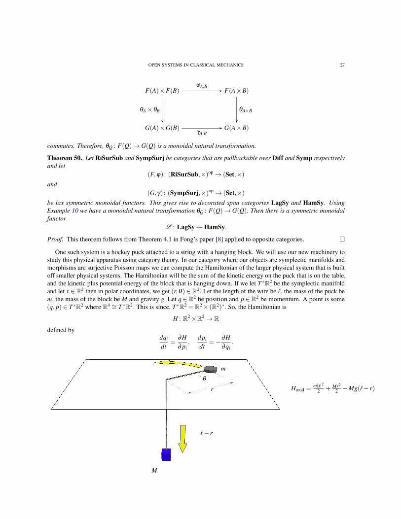
One such system is a hockey puck attached to a string with a hanging block. We will use our new machinery tostudy this physical apparatus using category theory. In our category where our objects are symplectic manifolds andmorphisms are surjective Poisson maps we can compute the Hamiltonian of the larger physical system that is builtoff smaller physical systems. The Hamiltonian will be the sum of the kinetic energy on the puck that is on the table,and the kinetic plus potential energy of the block that is hanging down. If we let T ∗R2 be the symplectic manifoldand let x ∈ R2 then in polar coordinates, we get (r,θ) ∈ R2. Let the length of the wire be `, the mass of the puck bem, the mass of the block be M and gravity g. Let q ∈ R2 be position and p ∈ R2 be momentum. A point is some(q, p) ∈ T ∗R2 where R4 ∼= T ∗R2. This is since, T ∗R2 = R2× (R2)∗. So, the Hamiltonian is

H : R2×R2→ R

defined bydqi

dt=

∂H∂ pi

,d pi

dt=−∂H

∂qi.

Htotal =m|x|2

2 + Mr2

2 −Mg(`− r)

θ

r

m

`− r

M


Hpuck =m|x|2

2

Hstring = 0

Hblock =Mr2

2−Mg(`− r)

If we look at the Hamiltonian of the system,

Htotal =m|x|2

2+

Mr2

2−Mg(`− r)

our goal is to determine Hamilton’s equations. So if we let

x =(

r cosθ

r sinθ

),

then

x =(

r cosθ − θr sinθ

r sinθ + θr cosθ

).


As a result,|x|2 = 〈x, x〉= r2 + θ

2r2.

Substituting this into Htotal

Htotal =m2(r2 + θ

2r2)+M2

r2−Mg(`− r) =m+M

2r2 +

m2

θ2r2−Mg(`− r).

By definition of the Lagrangian, which is the difference between the kinetic and potential energy we can write theLagrangian as

L =m+M

2r2 +

m2

θ2r2 +Mg(`− r).

Using the canonical positions q1,q2 and associated momenta p1, p2 choose q1 = r,q2 = θ then by the Euler-Lagrangeequations p j =

∂L∂ q j

. We should note that ∂L∂ q j

is the functional derivative. Then by definition of the functionalderivative we have the following:

p1 =∂L∂ q1

=∂L∂ r

= (m+M)r, p2 =∂L∂ q2

=∂L∂ θ

= mr2θ .

Hence, Hamilton’s equations are

q1 =∂H∂ p1

=1

m+Mp1, p1 =−

∂H∂ q1

=1m

q−31 p2

2−Mg

q2 =∂H∂ p2

=1

mr2 p1, p2 =−∂H∂ q2

= 0.

We should note that since p2 = 0 then p2 = mr2θ = constant. This shows that angular momentum is conserved.We can use category theory to model the physical apparatus of the system. In general if we have a composite of

spans we can find the Hamiltonians H,H ′ on S and S′ respectively. Then by definition Hamiltonian, we can find theHamiltonian on S×M′ S′ by taking

H ′′ = H πS +H ′ πS′ .

M M′ M′′

S S′

S×M′ S′

R

f g f ′ g′

πS′

H H ′H ′′

πS

T ∗M T ∗M T ∗M

T ∗M×T ∗M T ∗M×T ∗M

T ∗M×T∗M T ∗M

R

1

H H ′H ′′

1

Just like our example with the masses and springs, if we are given a string with no mass, we can find the Hamiltoniansfor the masses attached to the springs by looking at their phase spaces as diagrams of spans.Now if we apply this method to this system, we can model its configuration space in terms of composing three spanssince we have three objects that have a Hamiltoninan, namely the block, string and puck. The configuration space


for the block will be (−∞,0), while the puck will have a configuration space of R2. In addition, the configurationspace for the string is

Qstring = (a,b) ∈ R2|a2 +b2 < `2.

The morphsism π ′1 is defined as π ′1(a,b) = `−√

a2 +b2, and ι is the inclusion map. As a result, when we do apullback we get

(−∞,0)×(−∞,0) Qstring = (h,a,b) ∈ R2|h = `−√

a2 +b2 ∼= Qstring.

This is due to the fact that a pullback depends on (a,b). Similar constructions for the other pullbacks also yieldQstring.

(−∞,0) (−∞,0) R2 R2

(−∞,0) Qstring R2

Qstring Qstring

Qstring

1 1 π ′1 ι 1 1

If we take the differential, we get the following diagram, which gives rise to the Lagrangian

T (−∞,0) T (−∞,0) TR2 TR2

T (−∞,0) T Qstring TR2

T Qstring T Qstring

T Qstring

.

Then applying our functor L we get the following diagram whose apices are decorated by the Hamiltonian.

T ∗(−∞,0) T ∗(−∞,0) T ∗R2 T ∗R2

T ∗(−∞,0) T ∗Qstring T ∗R2

T ∗Qstring T ∗Qstring

T ∗Qstring

1 1 π ′1 ι 1 1

.

If we look at the pullback on the left side of the diagram, we see the following

T ∗(−∞,0) T ∗(−∞,0) T ∗R2

T ∗(−∞,0) T ∗Qstring

T ∗Qstring

1 1 π ′1 ι

.

The phase space of the block is the apex T ∗(−∞,0) whose Hamiltonian is Mr2

2 −Mg(`− r) and the phase spaceof the string is the apex T ∗Qstring whose Hamiltonian is 0. Therefore, using our defintion of the Hamiltonian on a


pullback we add the Hamiltonian of the block and string to get Mr2

2 −Mg(`− r). Repeating the same procedure forthe right side of the diagram, we have the following diagram

T ∗(−∞,0) T ∗R2 T ∗R2

T ∗Qstring T ∗R2

T ∗Qstring

π ′1 ι 1 1

.

The phase space for the puck is represented by the apex T ∗R2 whose Hamiltonian is m|x|22 . As a result, the

Hamiltonian for the pullback will be the sum of the Hamiltonian on the string and puck, which is m|x|22 . Therefore, if

we take the pullback over T ∗Qstring

T ∗(−∞,0) T ∗Qstring T ∗R2

T ∗Qstring T ∗Qstring

T ∗Qstring

and taking the sum of the Hamiltonians of the two apices then the pullback will have a Hamiltonian of m|x|22 + Mr2

2 −Mg(`− r).

9. ACKNOWLEDGEMENTS

First and foremost, I would like to offer my sincerest thanks to John Baez for his immense help and impactfulteaching methods from which I learned category theory and classical mechanics. He has taught me more than Icould ever give him credit for and I am grateful for his magnanimity, patience and masterful tutelage. I would alsolike to thank Daniel Cicala, Kenny Courser, Jason Erbele, John Simanyi and David Weisbart for their insight, aidand wonderful discussions we had. In addition, I also want to thank Brendan Fong for his work on the subject.Finally, I would like to thank Alan Weinstein for his helpful emails regarding Poisson geometry.

10. APPENDIX

For any object C ∈ C let Hom(C,−) be the hom functor that maps an object X to the set Hom(C,X). For us, wewill use Diff(C,−) and Diff(C,X) to denote the hom functor and hom set respectively in the category Diff.

Definition 51. Let C be a locally small category. A functor F : C→ Set is said to be representable if it is naturallyisomorphic to Hom(C,−) for some object C of C.

Representable functors have a nice property in that they preserve limits or pullbacks, which we now show usingF. Borceux’s proof in [4].

Proposition 52. Consider a category C and an object C ∈ C. The representable functor Hom(C,−) : C→ Setpreserves limits.

Proof. Consider a functor F : D→ C with limit (L,(pD)D∈D) and a cone (qD : M → Hom(C,FD))D∈D overHom(C,F−) in Set. For each element m ∈M, the family (qD(m) : C→FD)D∈D is a cone on F and thereforethere exits a unique morphism qD(m) : C→ L in C such that for each D ∈D, pD q(m) = qD(m). This defines amapping q : M→ Hom(C,L) with the property Hom(C, pD)q = qD for all D ∈D. The uniqueness of q followsfrom that of the q(m)’s.

Lemma 53. The forgetful functor U : Diff→ Set is representable.


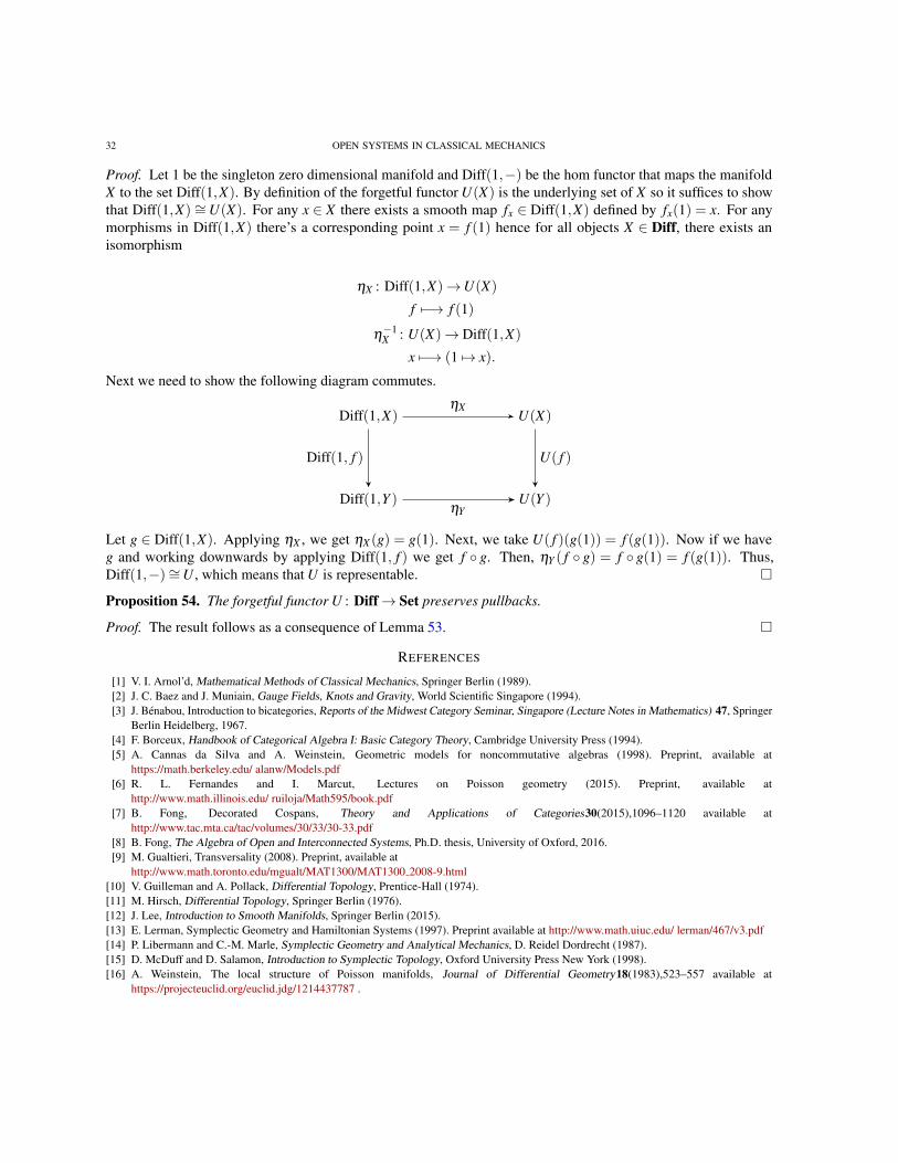
Proof. Let 1 be the singleton zero dimensional manifold and Diff(1,−) be the hom functor that maps the manifoldX to the set Diff(1,X). By definition of the forgetful functor U(X) is the underlying set of X so it suffices to showthat Diff(1,X) ∼= U(X). For any x ∈ X there exists a smooth map fx ∈ Diff(1,X) defined by fx(1) = x. For anymorphisms in Diff(1,X) there’s a corresponding point x = f (1) hence for all objects X ∈ Diff, there exists anisomorphism

ηX : Diff(1,X)→U(X)

f 7−→ f (1)

η−1X : U(X)→ Diff(1,X)

x 7−→ (1 7→ x).

Next we need to show the following diagram commutes.

Diff(1,Y )

Diff(1,X) U(X)

U(Y )

ηX

Diff(1, f ) U( f )

ηY

Let g ∈ Diff(1,X). Applying ηX , we get ηX (g) = g(1). Next, we take U( f )(g(1)) = f (g(1)). Now if we haveg and working downwards by applying Diff(1, f ) we get f g. Then, ηY ( f g) = f g(1) = f (g(1)). Thus,Diff(1,−)∼=U , which means that U is representable.

Proposition 54. The forgetful functor U : Diff→ Set preserves pullbacks.

Proof. The result follows as a consequence of Lemma 53.

REFERENCES

[1] V. I. Arnol’d, Mathematical Methods of Classical Mechanics, Springer Berlin (1989).[2] J. C. Baez and J. Muniain, Gauge Fields, Knots and Gravity, World Scientific Singapore (1994).[3] J. Benabou, Introduction to bicategories, Reports of the Midwest Category Seminar, Singapore (Lecture Notes in Mathematics) 47, Springer

Berlin Heidelberg, 1967.[4] F. Borceux, Handbook of Categorical Algebra I: Basic Category Theory, Cambridge University Press (1994).[5] A. Cannas da Silva and A. Weinstein, Geometric models for noncommutative algebras (1998). Preprint, available at

https://math.berkeley.edu/ alanw/Models.pdf[6] R. L. Fernandes and I. Marcut, Lectures on Poisson geometry (2015). Preprint, available at

http://www.math.illinois.edu/ ruiloja/Math595/book.pdf[7] B. Fong, Decorated Cospans, Theory and Applications of Categories30(2015),1096–1120 available at

http://www.tac.mta.ca/tac/volumes/30/33/30-33.pdf[8] B. Fong, The Algebra of Open and Interconnected Systems, Ph.D. thesis, University of Oxford, 2016.[9] M. Gualtieri, Transversality (2008). Preprint, available at

http://www.math.toronto.edu/mgualt/MAT1300/MAT1300 2008-9.html[10] V. Guilleman and A. Pollack, Differential Topology, Prentice-Hall (1974).[11] M. Hirsch, Differential Topology, Springer Berlin (1976).[12] J. Lee, Introduction to Smooth Manifolds, Springer Berlin (2015).[13] E. Lerman, Symplectic Geometry and Hamiltonian Systems (1997). Preprint available at http://www.math.uiuc.edu/ lerman/467/v3.pdf[14] P. Libermann and C.-M. Marle, Symplectic Geometry and Analytical Mechanics, D. Reidel Dordrecht (1987).[15] D. McDuff and D. Salamon, Introduction to Symplectic Topology, Oxford University Press New York (1998).[16] A. Weinstein, The local structure of Poisson manifolds, Journal of Differential Geometry18(1983),523–557 available at

https://projecteuclid.org/euclid.jdg/1214437787 .

https://math.berkeley.edu/~alanw/Models.pdf

http://www.math.illinois.edu/~ruiloja/Math595/book.pdf

http://www.tac.mta.ca/tac/volumes/30/33/30-33.pdf

http://www.math.toronto.edu/mgualt/MAT1300/MAT1300_2008-9.html

http://www.math.uiuc.edu/~lerman/467/v3.pdf

https://projecteuclid.org/euclid.jdg/1214437787

OPEN SYSTEMS IN CLASSICAL MECHANICS Adam … · OPEN SYSTEMS IN CLASSICAL MECHANICS Adam Yassine...

Documents

Transcript of OPEN SYSTEMS IN CLASSICAL MECHANICS Adam … · OPEN SYSTEMS IN CLASSICAL MECHANICS Adam Yassine...