Op Tim Ization
310
NX Nastran Design Sensitivity and Optimization User’s Guide
-
Upload
redoctober24 -
Category
Documents
-
view
958 -
download
0
Transcript of Op Tim Ization

NX Nastran Design Sensitivity andOptimization User’s Guide

Proprietary & Restricted Rights Notice
© 2007 UGS Corp. All Rights Reserved. This software and related documentation are proprietaryto UGS Corp.
NASTRAN is a registered trademark of the National Aeronautics and Space Administration. NXNastran is an enhanced proprietary version developed and maintained by UGS Corp.
MSC is a registered trademark of MSC.Software Corporation. MSC.Nastran and MSC.Patranare trademarks of MSC.Software Corporation.
All other trademarks are the property of their respective owners.
2 NX Nastran Design Sensitivity and Optimization User’s Guide

Contents
Getting Started . . . . . . . . . . . . . . . . . . . . . . . . . . . . . . . . . . . . . . . . . . . . . . . . . . . . . 1-1
Introduction . . . . . . . . . . . . . . . . . . . . . . . . . . . . . . . . . . . . . . . . . . . . . . . . . . . . . . . . 1- 2Numerical Optimization Basics . . . . . . . . . . . . . . . . . . . . . . . . . . . . . . . . . . . . . . . . . . 1- 7Structural Optimization . . . . . . . . . . . . . . . . . . . . . . . . . . . . . . . . . . . . . . . . . . . . . . . 1-19
Design Modeling for Sensitivity and Optimization . . . . . . . . . . . . . . . . . . . . . . . . . . 2-1
Overview of Design Modeling . . . . . . . . . . . . . . . . . . . . . . . . . . . . . . . . . . . . . . . . . . . . 2- 2Defining the Analysis Disciplines . . . . . . . . . . . . . . . . . . . . . . . . . . . . . . . . . . . . . . . . . 2- 3Defining the Design Variables . . . . . . . . . . . . . . . . . . . . . . . . . . . . . . . . . . . . . . . . . . . 2- 5Relating Design Variables to Properties . . . . . . . . . . . . . . . . . . . . . . . . . . . . . . . . . . . . 2- 8Relating Design Variables to Shape Changes . . . . . . . . . . . . . . . . . . . . . . . . . . . . . . . . . 2-19Identifying the Design Responses . . . . . . . . . . . . . . . . . . . . . . . . . . . . . . . . . . . . . . . . . 2-39Defining the Objective Function . . . . . . . . . . . . . . . . . . . . . . . . . . . . . . . . . . . . . . . . . . 2-47Defining the Constraints . . . . . . . . . . . . . . . . . . . . . . . . . . . . . . . . . . . . . . . . . . . . . . . 2-48Superelement Design Modeling . . . . . . . . . . . . . . . . . . . . . . . . . . . . . . . . . . . . . . . . . . 2-52
Design Sensitivity and Optimization in NX Nastran . . . . . . . . . . . . . . . . . . . . . . . . . 3-1
Approximation Concepts in Design Optimization . . . . . . . . . . . . . . . . . . . . . . . . . . . . . . 3- 2Design Sensitivity Analysis . . . . . . . . . . . . . . . . . . . . . . . . . . . . . . . . . . . . . . . . . . . . . 3-22Optimization with Respect to Approximate Models . . . . . . . . . . . . . . . . . . . . . . . . . . . . . 3-40Convergence Tests . . . . . . . . . . . . . . . . . . . . . . . . . . . . . . . . . . . . . . . . . . . . . . . . . . . . 3-50
Input Data . . . . . . . . . . . . . . . . . . . . . . . . . . . . . . . . . . . . . . . . . . . . . . . . . . . . . . . . . 4-1
File Management Section, Executive Control . . . . . . . . . . . . . . . . . . . . . . . . . . . . . . . . . 4- 2Case Control Section . . . . . . . . . . . . . . . . . . . . . . . . . . . . . . . . . . . . . . . . . . . . . . . . . . 4- 3Bulk Data Entries . . . . . . . . . . . . . . . . . . . . . . . . . . . . . . . . . . . . . . . . . . . . . . . . . . . . 4- 6Parameters for Design Sensitivity and Optimization . . . . . . . . . . . . . . . . . . . . . . . . . . . 4-23
Output Features and Interpretation . . . . . . . . . . . . . . . . . . . . . . . . . . . . . . . . . . . . . 5-1
Output-Controlling Parameters . . . . . . . . . . . . . . . . . . . . . . . . . . . . . . . . . . . . . . . . . . 5- 2Design Optimization Output . . . . . . . . . . . . . . . . . . . . . . . . . . . . . . . . . . . . . . . . . . . . 5- 3Design Sensitivity Output . . . . . . . . . . . . . . . . . . . . . . . . . . . . . . . . . . . . . . . . . . . . . . 5-12
Solution Sequences . . . . . . . . . . . . . . . . . . . . . . . . . . . . . . . . . . . . . . . . . . . . . . . . . . 6-1
Design Sensitivity and Optimization Modules . . . . . . . . . . . . . . . . . . . . . . . . . . . . . . . . 6- 2Selected Data Blocks . . . . . . . . . . . . . . . . . . . . . . . . . . . . . . . . . . . . . . . . . . . . . . . . . . 6- 4Solution 200 Program Flow . . . . . . . . . . . . . . . . . . . . . . . . . . . . . . . . . . . . . . . . . . . . . 6- 8
Example Problems . . . . . . . . . . . . . . . . . . . . . . . . . . . . . . . . . . . . . . . . . . . . . . . . . . . 7-1
Three-Bar Truss . . . . . . . . . . . . . . . . . . . . . . . . . . . . . . . . . . . . . . . . . . . . . . . . . . . . . 7- 3Vibration of a Cantilever Beam (Turner’s Problem) . . . . . . . . . . . . . . . . . . . . . . . . . . . . 7- 8Cantilevered Plate . . . . . . . . . . . . . . . . . . . . . . . . . . . . . . . . . . . . . . . . . . . . . . . . . . . 7-11
NX Nastran Design Sensitivity and Optimization User’s Guide 3

Contents
Stiffened Plate . . . . . . . . . . . . . . . . . . . . . . . . . . . . . . . . . . . . . . . . . . . . . . . . . . . . . . 7-16Shape Optimization of a Culvert . . . . . . . . . . . . . . . . . . . . . . . . . . . . . . . . . . . . . . . . . . 7-24Analytic Boundary Shapes . . . . . . . . . . . . . . . . . . . . . . . . . . . . . . . . . . . . . . . . . . . . . . 7-30Dynamic Response Optimization . . . . . . . . . . . . . . . . . . . . . . . . . . . . . . . . . . . . . . . . . 7-38Twenty-Five Bar Truss, Superelement Optimization . . . . . . . . . . . . . . . . . . . . . . . . . . . 7-45Design Optimization with Composite Materials . . . . . . . . . . . . . . . . . . . . . . . . . . . . . . . 7-52Acoustic Optimization . . . . . . . . . . . . . . . . . . . . . . . . . . . . . . . . . . . . . . . . . . . . . . . . . 7-57Restarts in Design Optimization . . . . . . . . . . . . . . . . . . . . . . . . . . . . . . . . . . . . . . . . . . 7-63
Glossary of Terms . . . . . . . . . . . . . . . . . . . . . . . . . . . . . . . . . . . . . . . . . . . . . . . . . . . A-1
Nomenclature . . . . . . . . . . . . . . . . . . . . . . . . . . . . . . . . . . . . . . . . . . . . . . . . . . . . . . B-1
Commonly Used Commands for Design Optimization . . . . . . . . . . . . . . . . . . . . . . . C-1
Bulk Data Entries . . . . . . . . . . . . . . . . . . . . . . . . . . . . . . . . . . . . . . . . . . . . . . . . . . . . C- 1Parameters . . . . . . . . . . . . . . . . . . . . . . . . . . . . . . . . . . . . . . . . . . . . . . . . . . . . . . . . . C- 1
Numerical Optimization . . . . . . . . . . . . . . . . . . . . . . . . . . . . . . . . . . . . . . . . . . . . . D-1
Introduction . . . . . . . . . . . . . . . . . . . . . . . . . . . . . . . . . . . . . . . . . . . . . . . . . . . . . . . . D- 1The Modified Feasible Direction Algorithm . . . . . . . . . . . . . . . . . . . . . . . . . . . . . . . . . . D- 8Finding the Search Direction . . . . . . . . . . . . . . . . . . . . . . . . . . . . . . . . . . . . . . . . . . . . D- 9Finding Bounds On α* . . . . . . . . . . . . . . . . . . . . . . . . . . . . . . . . . . . . . . . . . . . . . . . . . D-19Interpolation for α* . . . . . . . . . . . . . . . . . . . . . . . . . . . . . . . . . . . . . . . . . . . . . . . . . . . D-20Convergence to the Optimum . . . . . . . . . . . . . . . . . . . . . . . . . . . . . . . . . . . . . . . . . . . . D-23Maximum Iterations . . . . . . . . . . . . . . . . . . . . . . . . . . . . . . . . . . . . . . . . . . . . . . . . . . D-23No Feasible Solution . . . . . . . . . . . . . . . . . . . . . . . . . . . . . . . . . . . . . . . . . . . . . . . . . . D-23Point of Diminishing Returns . . . . . . . . . . . . . . . . . . . . . . . . . . . . . . . . . . . . . . . . . . . . D-23Satisfaction of the Kuhn-Tucker Conditions . . . . . . . . . . . . . . . . . . . . . . . . . . . . . . . . . . D-24Sequential Linear Programming . . . . . . . . . . . . . . . . . . . . . . . . . . . . . . . . . . . . . . . . . . D-24Sequential Quadratic Programming . . . . . . . . . . . . . . . . . . . . . . . . . . . . . . . . . . . . . . . D-27Summary . . . . . . . . . . . . . . . . . . . . . . . . . . . . . . . . . . . . . . . . . . . . . . . . . . . . . . . . . . D-28
4 NX Nastran Design Sensitivity and Optimization User’s Guide

Chapter
1 Getting Started
• Introduction
• Numerical Optimization Basics
• Structural Optimization
NX Nastran Design Sensitivity and Optimization User’s Guide 1-1

Chapter 1 Getting Started
1.1 IntroductionThis chapter introduces some of the basic concepts of numerical optimization with an emphasison the methods used in NX Nastran.
Some of the questions answered in this chapter include:
• What is design optimization, and how does it differ from analysis?
• What is the relationship between design sensitivity and optimization?
• How is an optimization problem formulated?
• How does an optimizer search for an optimum?
• How does an optimizer communicate with the structural analysis?
If you are interested in seeing some complete example problems in connection with the materialcovered in this chapter, you may want to refer to the first couple of examples from ExampleProblems. You will probably also need to refer to the Bulk Data descriptions in the NX NastranQuick Reference Guide for the details of the entries used. Example Problems should help togive you some idea of what NX Nastran design optimization input and output looks like. Thedetails are covered in later chapters.
What is Design Sensitivity and Optimization?Design sensitivity and optimization are two separate, though closely related, topics.
Design sensitivity analysis computes the rates of change of structural responses with respectto changes in design parameters. These design parameters are usually referred to as designvariables and can be used to represent shell thicknesses, beam cross sectional dimensions,journal bearing sizes, and so on. In civil engineering, we may be interested in how changes in thedeflection of a bridge span can be affected by changes in the dimensions of the bridge sections. Inautomotive chassis design, we may want to investigate changes in cabin resonant frequenciesgiven changes in panel thicknesses. These rates of change (what we call “partial derivatives” inthe language of calculus) are called design sensitivity coefficients.
Design optimization refers to the process of generating improved designs. In NX Nastran, designoptimization is performed by an optimizer. An optimizer is really nothing more than a formalplan, or algorithm, that is used to search for a “best” design. Design sensitivity coefficients areused in NX Nastran to assist the optimizer in this search process. Once these rates of changeare known, the optimizer can, for example, find the optimal set of panel thicknesses that yieldthe lowest level of cabin resonant frequencies.
Read on to discover ways that design sensitivity and optimization can help you to generatebetter designs.
Why Use Design Sensitivity and Optimization?Why use design sensitivity and optimization? Perhaps you have been requested to investigateproduct improvement using optimization, or perhaps you are aware that these tools can be usedto create better engineered designs. Design sensitivity and optimization are used when we seekto modify a design whose level of structural complexity exceeds our ability to make appropriatedesign changes. What is surprising is that an extremely simple design task may easily surpassour decision-making abilities. Experienced designers, those with perhaps decades of experience,are sometimes fantastically adept at poring through mounds of data and coming up with
1-2 NX Nastran Design Sensitivity and Optimization User’s Guide

Getting Started
improved designs. Most of us, however, cannot draw upon such intuition and experience. A basicgoal of design optimization is to automate the design process by using a rational, mathematicalapproach to yield improved designs. Ways in which this might be put to use include:
1. Producing more efficient designs having maximum margins of safety.
2. Performing trade-off or feasibility studies.
3. Assisting in design sensitivity studies.
4. Correlating test data and analysis results (model matching).
In addition to providing a complete description of the optimization tools in NX Nastran, partof the aim of this user’s guide is to suggest various ways in which design sensitivity andoptimization might be used. Consider the following examples:
Example A
A complex spacecraft is in a conceptual design stage. The total weight of the spacecraft cannotexceed 3,000 pounds. The nonstructural equipment including the payload is 2,000 pounds. Staticloads are prescribed based on the maximum acceleration at launch. Also, the guidance systemsrequire that the fundamental elastic frequency must be above 12 Hz. It is extremely importantto reduce the structural weight since it costs several thousand dollars to place one pound of massin a low earth orbit. There are three types of proposed designs: truss, frame, and stiffenedshell configurations. Currently all of the designs fail to satisfy at least one design requirementand are expected to be overweight. We are to determine which configuration(s) promises thebest performance and warrants detailed design study. Also, the payload manager needs toknow how much weight could be saved if the frequency requirement were to be relaxed from 12Hz to 10 Hz. The spacecraft’s structure contains about 150 structural parameters, which wemay want to vary simultaneously.
Example B
One part of a vehicle’s frame structure was found to be overstressed. Unfortunately, it is tooexpensive to redesign that particular frame component at this stage in the engineering cycle.However, other structural components nearby can be modified without severe cost increases.There are nearly 100 structural design parameters that can be manipulated. The design goal is toreduce the magnitude of the stresses by reducing the internal load to the overstressed member.
Example C
A frame structure, which supports a set of sensitive instruments, must withstand severein-service dynamic loads. Modal test results are available from comprehensive tests performedon the prototype structure. We need to create a finite element model for dynamic analysis that ismuch less detailed than the original model created for stress analysis since the costs of dynamicanalysis using a complex model would be prohibitive. We must ensure, however, that the firstten modes obtained from our simplified model are in close agreement with those obtained fromthe test results. The goal is to determine suitable properties for the lumped quantities in oursimplified dynamic model so that the first ten eigenvalues correlate well with the prototype.
NX Nastran Design Sensitivity and Optimization User’s Guide 1-3
Chapter 1 Getting Started
How Does Design Optimization Differ from Analysis?
Although design optimization and analysis can be viewed as complementary, there are someimportant conceptual differences between the two that must be clear in order to make effectiveuse of both.
Analysis Models
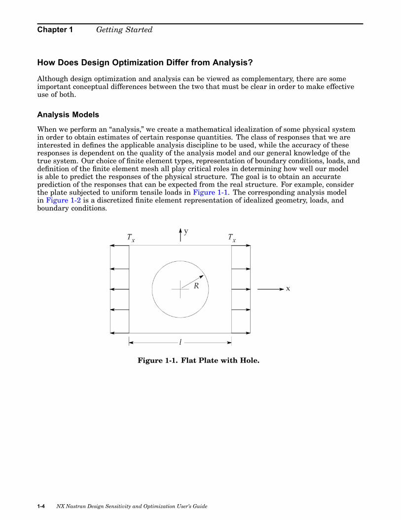
When we perform an “analysis,” we create a mathematical idealization of some physical systemin order to obtain estimates of certain response quantities. The class of responses that we areinterested in defines the applicable analysis discipline to be used, while the accuracy of theseresponses is dependent on the quality of the analysis model and our general knowledge of thetrue system. Our choice of finite element types, representation of boundary conditions, loads, anddefinition of the finite element mesh all play critical roles in determining how well our modelis able to predict the responses of the physical structure. The goal is to obtain an accurateprediction of the responses that can be expected from the real structure. For example, considerthe plate subjected to uniform tensile loads in Figure 1-1. The corresponding analysis modelin Figure 1-2 is a discretized finite element representation of idealized geometry, loads, andboundary conditions.
Figure 1-1. Flat Plate with Hole.
1-4 NX Nastran Design Sensitivity and Optimization User’s Guide
Getting Started
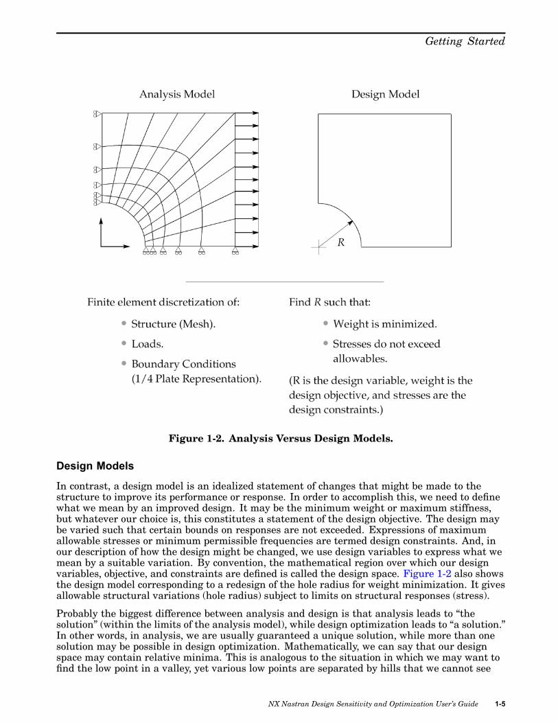
Figure 1-2. Analysis Versus Design Models.
Design Models
In contrast, a design model is an idealized statement of changes that might be made to thestructure to improve its performance or response. In order to accomplish this, we need to definewhat we mean by an improved design. It may be the minimum weight or maximum stiffness,but whatever our choice is, this constitutes a statement of the design objective. The design maybe varied such that certain bounds on responses are not exceeded. Expressions of maximumallowable stresses or minimum permissible frequencies are termed design constraints. And, inour description of how the design might be changed, we use design variables to express what wemean by a suitable variation. By convention, the mathematical region over which our designvariables, objective, and constraints are defined is called the design space. Figure 1-2 also showsthe design model corresponding to a redesign of the hole radius for weight minimization. It givesallowable structural variations (hole radius) subject to limits on structural responses (stress).
Probably the biggest difference between analysis and design is that analysis leads to “thesolution” (within the limits of the analysis model), while design optimization leads to “a solution.”In other words, in analysis, we are usually guaranteed a unique solution, while more than onesolution may be possible in design optimization. Mathematically, we can say that our designspace may contain relative minima. This is analogous to the situation in which we may want tofind the low point in a valley, yet various low points are separated by hills that we cannot see
NX Nastran Design Sensitivity and Optimization User’s Guide 1-5
Chapter 1 Getting Started
over. Simply finding a low point itself represents an acceptable solution, but there may bemore than one such solution. In some instances we may be able to restate the problem and, ineffect, shift the locations and contours of the hills to allow more efficient convergence. However,the fact remains that our goal has been stated in the context of design improvement and notin determining a unique solution (as in the case of analysis).
Integrity of Analysis and Design Modes
One thing the analysis and design models share is that the results are dependent upon the skilland judgement used in their construction. A poorly-meshed finite element model may lead toinaccurate and misleading results. Similarly, an ill-posed design optimization task may produceunexpected or useless results. Since the redesign process is based on analysis results, the resultsof design optimization are strongly dependent on the integrity of the analysis model.
Optimizer Limitations
A numerical optimizer seeks to find an improved design by trying to minimize or maximize aprespecified objective. Throughout this process, it must adhere to the bounds on responses anddesign variables given in the design model. It does not have the intelligence to modify theobjective or relax any of these limits. For example, suppose you asked a friend to find you a niceapartment on his street. Your friend, the optimizer, may have a somewhat different definitionof “nice” than you do. His income might be higher than yours, so that the optimal design heproposes may be infeasible in terms of your bank account. Even though he is searching just on hisstreet, the next block may turn out to have an apartment that you consider a better value. Theoptimizer is not able to go beyond your specifications to search out other possible configurations.
The optimization problem statement requires an explicit description of the design objective, aswell as bounds that define the region in which it may search. You may ask for a design satisfyinga minimum flexibility requirement such as wing tip deflection, but without a weight budget, thedesign that the optimizer proposes may turn out to be unrealistic. You might get an extremelystiff, 200 ton wing out of this process. You also might have asked for a minimum weight designbut allowed for negative physical dimensions. The optimizer may have no trouble minimizingthe weight by adding negative mass, but this design may produce a true engineering challengeon the factory floor.
An optimizer is only able to search for your definition of a best design within the region you havedefined. Configuration or trade-off studies cannot be directly addressed by a numerical optimizer,although an optimizer can be used to investigate the benefits of one design over another. Anoptimizer cannot weigh the benefits of a cast aluminum versus a welded steel support member,but it can tell you the best that each design is capable of and then let you decide which designpath to pursue. Some of these considerations are, in fact, active areas of research. Even withthese limitations, design optimization offers an extremely powerful set of design tools.
What Do I Need to Use Design Optimization Effectively?
Analysis Skills
Since design sensitivity and optimization depends on the results of analysis, a reasonablelevel of skill preparing NX Nastran analysis models is required. Design optimization can useanalysis results from statics, normal modes, buckling, direct and modal frequency, modaltransient, acoustic, and aeroelastic response analysis. In addition, design models can also employsuperelements. Proficiency in any or all of these disciplines is useful.
1-6 NX Nastran Design Sensitivity and Optimization User’s Guide

Getting Started
Material Presented in This Guide, and Other ResourcesThe topics covered in this user’s guide are intended to describe design sensitivity and optimizationin NX Nastran. No prior knowledge of structural optimization is required. This guide attemptsto describe all aspects completely so that someone new to the field of design optimization, as wellas those with more experience, have enough information available to use it wisely and effectively.
Engineering Judgement and Common SenseProbably the most critical requirement in the effective use of design optimization is commonsense. Any sufficiently general and powerful tool possesses the capacity for misuse. Thisis especially true of numerical optimizers. The old adage that engineering is more art thanscience is probably more true of design optimization than of many other disciplines. As yougain experience with numerical optimization, you will probably discover a few pitfalls that areparticular to your fields of application, and in the process you may discover some especiallyuseful and efficient “tricks” for clearly stating your optimization tasks. In any field of application,there is no substitute for a well-posed problem. If your design goals are clear, the constraints aremeaningful and well-conditioned, and the design variables are chosen carefully to produce usefuldesigns, then success becomes more certain. The description of methods for accomplishing thesegoals forms the majority of the material of this guide. Before moving on to a detailed discussionof NX Nastran design optimization in Design Modeling for Sensitivity and Optimization andDesign Sensitivity and Optimization in NX Nastran, the next two sections introduce some of thebasic concepts of numerical optimizers and how they are used to solve problems in structuraloptimization.
1.2 Numerical Optimization BasicsThis section introduces some of the basics of numerical optimization in an intuitive manner,stressing overall concepts over technical details. Since few universities include designoptimization in their curricula, this section may be a useful introduction to numericaloptimization for those entirely new to the subject. Once the basics of numerical optimization havebeen covered, Structural Optimization introduces the extension of these methods to the field ofstructural design. These sections in combination should provide adequate preparation for DesignModeling for Sensitivity and Optimization, which discusses design modeling in NX Nastran.
How Much Do I Need to Know About Optimizers?The safest answer to this question is, “The more you know about numerical optimizers, the betteroff you are.” This answer does not imply that you must be an expert in numerical optimizationtechniques in order to use those implemented in NX Nastran. In fact, it would be nice if designoptimization were such an automatic procedure that all an engineer had to do was to push the“optimization button” and an optimal design would result.
Some knowledge of the basic procedures involved in numerical optimizers will aid inunderstanding why an optimizer does what it does, in interpreting the final results of anoptimization run, and in understanding what may have happened if the results are unexpected.For example, it is not necessary to know all of the details of sparse matrix decomposition inorder to perform a linear static finite element analysis, but if singularities are present in yourmodel and the decomposition procedure fails, the results are far less mystifying, and a modelingsolution to the problem may be much more apparent if you know something of the basics of thesolution procedure. Most of the parameters that control the optimizer in NX Nastran can bechanged to improve performance for various classes of problems. Understanding the significanceof these choices allows you to take full advantage of the tools at your disposal.
NX Nastran Design Sensitivity and Optimization User’s Guide 1-7

Chapter 1 Getting Started
Design Optimization and Operations Research
Design optimization in structural redesign is actually an application of operations research (abranch of applied mathematics) to problems in engineering design. Generally, these are classesof problems in which the optimum allocation of scarce resources is desired. Operations researchis frequently used to solve scheduling problems such as the routing of airplanes among variousairport facilities. The allocation of 100 airplanes among 68 airports may not seem to have muchto do with engineering design, but the optimization methods employed are similar and can beextended to structural problems. An efficient engineering solution to a design problem involvesthe optimum allocation of scarce resources. For example, tensile stresses cannot be allowed toassume unlimited values and must be restricted to within reasonable limits (the distribution ofstrain energy density must be made in an optimal manner). Likewise, reducing structural massleads to a savings of material and possibly maintenance, fuel, or other indirect costs.
The Basic Optimization Problem Statement
Before introducing any formal relations, assume that we are assigned the type of task that anumerical optimizer might be asked to solve. We must examine ways to approach the problem.From this experience, we can build the equations that describe the basic optimization problemstatement.
Objective and Constraint Functions, Design Spaces
Suppose we are standing on the side of a hill and would like to find the point of lowest elevation;this is our “objective.” Suppose also that some fences exist that force us to restrict our search towithin the region enclosed by these fences. These fences or “constraints” act as bounds in our“design space,” which is the region that defines all of our possible positions on the hill. Onlyone out of all points on the hill can be considered an optimum, though. For simplicity, we areneglecting the presence of relative minima.
Finding the lowest point on the hill while staying inside the fences is no real problem. All wereally need to do is have a good look about and note, from our perspective, which point on the hillappears to be the lowest. We have scanned the hill, analyzed thousands of possible candidates ata glance, and made an immediate decision. If we were blindfolded, though, our decision-makingprocess would not be as simple, and that is exactly the task a numerical optimizer is faced with.
In a computational sense, the elevation of a single point on the hill, or the numerical valueof our objective function, must be determined by an analysis that may take considerableeffort. Evaluating hundreds or thousands of candidate designs may be prohibitive. We need asystematic method of searching for an optimal design. There are numerous techniques availableto solve such a problem, all of which are classified as numerical optimization algorithms.
Search Directions Based on Gradient Information
Generally, numerical optimization methods seek to determine a direction of travel or “searchdirection” that moves us down the hill as quickly as possible, yet allows us to find an optimumthat lies within the fences. A sequence of search directions is usually employed during theoverall search procedure.
In our hill example, we could easily find a search direction, even though blindfolded, by takingsmall steps from side to side and then forward and back to test for elevation changes. Basedon this estimate of a downhill direction, we can then proceed until we hit a fence or the hillstarts to climb up again. What we have done is to find the local value of the “gradient” of ourobjective function and then used this information to establish a probable direction in which tosearch for a minimum. Numerical optimization algorithms that rely on gradient information are
1-8 NX Nastran Design Sensitivity and Optimization User’s Guide

Getting Started
termed “gradient-based.” Once we have done the best we can possibly do in this direction, we findanother search direction, and again proceed as before. We continue to repeat this procedure untilwe cannot reduce the objective function any further.
Design Variables, Constrained, and Unconstrained Problems
To quantify the location of a point on the hill, we might use north-south and east-westcoordinates corresponding to the elevation at a given point. In design optimization terms, this isa two “design variable” space since two coordinate values are required to uniquely specify a pointin the design space. Two design variables are the most we can easily visualize. Considering thatan optimizer may have to deal with tens or even hundreds of design variables, the task becomesunderstandably more complex. We might also have the condition that fences, or constraints, donot exist or are located so far “uphill” that they do not affect our search for a minimum. Thissituation is an unconstrained optimization task in contrast to a constrained task.
Equality Constraints
We might also have the condition that we want the design to lie on some prescribed path or curvedrawn on the hillside. This is an equality constraint. Note that if there are as many equalityconstraints as design variables, a unique solution exists (as long as the equalities are linearlyindependent). This solution can be found using standard algebraic methods. A finite elementanalysis belongs to this category of problem. When the number and type of constraints do notenable a direct, unique solution, the job becomes complex and numerical optimizers must be used.
The Basic Optimization Problem Statement
We are now in a position to express our optimization task in a quantitative form. Thismathematical expression of the design problem is called the basic optimization problemstatement and can be written as follows:
minimize
Equation 1-1.
subject to
Equation 1-2.
Equation 1-3.
NX Nastran Design Sensitivity and Optimization User’s Guide 1-9

Chapter 1 Getting Started
Equation 1-4.
where:
Equation 1-5.
Function Minimization MaximizationThe objective function is the scalar quantity to be minimized. It is a function of the set of designvariables. (Although we stated the problem as a minimization task, we can easily maximize afunction by minimizing its negative.) Side constraints are placed on the design variables to limitthe region of search, for example, to plate thicknesses that are nonnegative or tubes whose wallthicknesses are less than one-tenth of the outer radii. The inequality constraints represent thefences on the hill and are expressed in a less than or equal to zero form by convention. We havesatisfied a constraint and are thus within the boundary defined by the fence if the constraint’svalue is negative. We have violated the constraint if its value is positive. The location of the
j-th “fence” lies at . Equality constraints, if present, must be satisfied exactly at theoptimal design.
Linear Versus Nonlinear ProblemsThe objective and constraint functions may either be linear or nonlinear functions of the designvariables. If all of these functions are linear, we may use linear techniques to find an optimalsolution if one exists. If just one of these functions is nonlinear, then search algorithms that candeal with this nonlinearity must be used. NX Nastran includes capabilities for solving bothlinear and nonlinear optimization problems.
As seen throughout the remainder of this user’s guide, the basic optimization problem statementis used directly in NX Nastran and influences the nomenclature adopted here. For example,the design objective is defined in the Case Control Section by the DESOBJ command, whilethe design variables and constraints are defined in the Bulk Data Section using the DESVARand DCONSTR entries respectively. We will see how these are used in Design Modeling forSensitivity and Optimization.
In conjunction with problems in structural optimization, we will discuss design spaces, objectives,constraints, and design variables. It is useful to take a look at a simple problem that is notexplicitly related to structural optimization, just to become familiar with these concepts.
ExampleConsider the following optimization problem:
minimize the objective:
Equation 1-6.
1-10 NX Nastran Design Sensitivity and Optimization User’s Guide

Getting Started
subject to the constraints:
Equation 1-7.
Equation 1-8.
Feasible Designs
The objective and constraint functions are dependent on two design variables x1 and x2. The
objective is linear in the design variables, while the constraint is nonlinear. Figure1-3 shows the two variable design space, where shading is used to denote regions in whichthe constraint or side constraints on the design variables are violated. If no constraints areviolated, we say the current design is feasible (although it is probably not optimal). A designis infeasible if one or more of the constraints are violated. For example, the point (2,2) is afeasible design, whereas the point (0.05,3) violates not only the inequality constraint but alsothe lower bound constraint on x1.
Figure 1-3. Two-Variable Function Space.
The optimal design at (1,1) can be found by inspection. The explicit description of the designproblem has allowed a graphical solution in two dimensions. In practice, we usually have morethan two design variables and non-explicit constraints and objective function. This complexityrequires an efficient searching procedure, recalling that the optimizer is essentially “blindfolded.”
NX Nastran Design Sensitivity and Optimization User’s Guide 1-11

Chapter 1 Getting Started
Numerically Searching for an Optimum
Gradient-Based AlgorithmsThe optimization algorithms in NX Nastran belong to the family of methods generally referred toas “gradient-based,” since, in addition to function values, they use function gradients to assist inthe numerical search for an optimum.
The numerical search process can be summarized as follows: for a given point in the designspace, we determine the gradients of the objective function and constraints and use thisinformation to determine a direction in which to search. We then proceed in this direction foras far as we can go, whereupon we investigate to see if we are at an optimum point. If we arenot, we repeat the process until we can make no further improvement in our objective withoutviolating any of the constraints.
Essentially this is the procedure used by the optimizer in NX Nastran, although the task iscomplicated by the structural optimization context. Here, we consider each of the aspects of thisprocess in more detail, with an emphasis placed on the intuitive aspects rather than a rigorousmathematical treatment.
Finite Difference Gradient ApproximationsThe first step in a numerical search procedure is determining the direction to search. Thesituation may be somewhat complicated if the current design is infeasible (one or more violatedconstraints) or if one or more constraints are critical. For an infeasible design, we are outside ofone of the fences, to use the hill analogy. For a critical design, we are standing right next to afence. In general, we at least need to know the gradient of our objective function and perhapssome of the constraint functions as well. The process of taking small steps in each of the designvariable directions (suppose we are not restricted by the fences for this step) corresponds exactlyto the mathematical concept of a first-forward finite difference approximation of a derivative. Fora single independent variable the first-forward difference is given by
Equation 1-9.
where the quantity Δx represents the small step taken in the direction x. For most practicaldesign tasks, we are usually concerned with a vector of design variables. The resultant vector ofpartial derivatives, or gradient, of the function can be written as
Equation 1-10.
1-12 NX Nastran Design Sensitivity and Optimization User’s Guide

Getting Started
where each partial derivative is a single component of the dimensional vector.
Details of how NX Nastran computes sensitivities can be found in Design SensitivityAnalysis.
Direction of Steepest Descent
Physically, the gradient vector points uphill, or in the direction of increasing objective function.If we want to minimize the objective function, we will actually move in a direction opposite tothat of the gradient. The steepest descent algorithm searches in the direction defined by thenegative of the objective function gradient, or
Equation 1-11.
since proceeding in this direction reduces the function value most rapidly. is referred to asthe search vector.
For now, just note that NX Nastran uses the steepest descent direction only when none of theconstraints are critical or violated and then only as the starting point for other, more efficientsearch algorithms. The difficulty in practice stems from the fact that, although the direction ofsteepest descent is usually a very good starting point, subsequent search directions often failto improve the objective function significantly. In NX Nastran we use other, more efficientmethods that can be generalized for the cases of active and/or violated constraints. We willbriefly introduce these methods later in this section. The next question to consider is: once wehave determined a search direction, how can this be used to improve our design?
One-Dimensional Search
Just as in the hill example, once we found a search direction, we proceeded “downhill” until webumped into a fence or until we reached the lowest point along our current path. Note that thisrequires us to take a number of steps in this given direction, which is equivalent to a number of
function evaluations in numerical optimization. For a search direction and a vector of designvariables , the new design at the conclusion of our search in this direction can be written as
Equation 1-12.
This relation allows us to update a potentially huge number of design variables by varyingthe single parameter α. We have been able to reduce the dimensionality from n to 1, that is,from n design variables to a single search parameter α. For this reason, this process is called aone-dimensional search. When we can no longer proceed in this search direction, we have thevalue of α, which represents the move required to reach the best design possible for this particulardirection. This value is defined as α*. The new objective and constraints can now be expressed as
NX Nastran Design Sensitivity and Optimization User’s Guide 1-13

Chapter 1 Getting Started
Equation 1-13.
Equation 1-14.
From this new point in the design space, we can again compute the gradients and establishanother search direction based on this information. Again, we will proceed in this new directionuntil no further improvement can be made, repeating the process, if necessary.
At some point we will not be able to establish a search direction that can yield an improveddesign. We may be at the bottom of the hill, or we may have proceeded as far as possible withoutcrossing over a fence. In the numerical search algorithm, it is necessary to have some formaldefinition of an optimum. Any trial design can then be measured against this criteria to see if itis met and an optimum has been found. This required definition is provided by the Kuhn-Tuckerconditions that are physically quite intuitive.
Convergence to an Optimum: The Kuhn-Tucker Conditions
Figure 1-4 shows a two design variable space with constraints and and objectivefunction . The constraint boundaries are those curves for which the constraint values areidentically zero. A few contours of constant objective are shown as well; these can be thought ofas contour lines drawn along constant elevations of the hill. The optimum point in this example
is the point that lies at the intersection of the two constraints. This location is shown as .
Figure 1-4. Kuhn-Tucker Condition at a Constrained Optimum.
1-14 NX Nastran Design Sensitivity and Optimization User’s Guide

Getting Started
If we compute the gradients of the objective and the two active constraints at the optimum, wesee that they all point off roughly in different directions. (Remember that function gradientspoint in the direction of increasing function values.) For this situation-a constrained optimum-theKuhn-Tucker conditions state that the vector sum of the objective and all active constraints mustbe equal to zero given an appropriate choice of multiplying factors. These factors are calledthe Lagrange multipliers. (Constraints that are not active at the proposed optimum are notincluded in the vector summation.) Indeed, Figure 1-5 shows this to be the case where λ1 andλ2 are the values of the Lagrange multipliers that enable the zero vector sum condition to bemet. We could probably convince ourselves that this condition could not be met for any otherpoint in this design space.
Figure 1-5. Graphical Interpretation of Kuhn-Tucker Conditions.
The Kuhn-Tucker conditions are useful even if there are no active constraints at the optimum. Inthis case, only the objective function gradient is considered, and this is identically equal to zero;i.e., any finite move in any direction will not decrease the objective function. A zero objectivefunction gradient indicates a stationary condition.
Not only are the Kuhn-Tucker conditions useful in determining if we have achieved an optimaldesign; they are also physically intuitive. The optimizer in NX Nastran tests the Kuhn-Tuckerconditions in connection with the search direction determination algorithm. The interestedreader can find the theoretical details in Appendix D.
A Simple Structural Example
In this section we covered the basic optimization problem statement, the concept of a designspace, gradient-based search techniques, and the meaning of an optimum in terms of satisfyingthe Kuhn-Tucker conditions. We pause here to take a look at a simple example to help fit thesepieces together and to introduce some qualitative aspects of the optimizer used in NX Nastran.
The cantilever beam in Figure 1-6 has a rectangular cross section. Suppose we want to minimizethe volume, and thus the weight of the beam, subject to constraints on maximum bending stressand deflection due to the tip loading. In addition, the beam’s cross section must remain belowa maximum beam height-to-width ratio to guard against the introduction of twisting modesof failure.
NX Nastran Design Sensitivity and Optimization User’s Guide 1-15

Chapter 1 Getting Started
Figure 1-6. Cantilever Beam.
The optimization problem statement could be written as follows:
minimize
Equation 1-15.
subject
Equation 1-16.
Equation 1-17.
Equation 1-18.
Equation 1-19.
Equation 1-20.
Since the objective and constraints are available explicitly, we can graphically display thetwo-variable design space as shown in Figure 1-7.
1-16 NX Nastran Design Sensitivity and Optimization User’s Guide

Getting Started
Figure 1-7. Cantilever Beam Design Space.
In Figure 1-7, note that the optimum lies at the vertex formed by the intersections of the beambending stress constraint and the constraint on maximum allowable ratio of cross-sectionalheight to width. This optimum occurs at an objective of approximately 1,000 cm3. Let us examinethe path that the optimizer might take as it searches for this constrained minimum.
Assume that we begin with an initial design of H = 44 cm and B = 7 cm. Since none of theconstraints are active, the direction of steepest descent is used as an initial search direction, andthe optimizer proceeds in this direction until it encounters a constraint boundary. From Figure1-8 we see that the structural volume cannot be reduced any further in this search directionwithout violating the maximum allowable tip deflection requirement. The optimizer is now facedwith a choice. A finite move in the direction of steepest descent would not be admissible sinceconstraints would then be violated, yet we know that the objective function can still be reduced.
NX Nastran Design Sensitivity and Optimization User’s Guide 1-17

Chapter 1 Getting Started
Figure 1-8. Sequence of Iterations: Modified Method of Feasible Directions.
The optimizer in NX Nastran resolves the situation by choosing a search vector that effectivelyfollows the active constraint boundary in the direction of decreasing objective function. (If theoptimizer could not find any direction in which to move, an optimum would be at hand since theKuhn-Tucker conditions have implicitly been satisfied.) The objective can be reduced furtherand we observe that by the time two such iterations have been completed, the true optimumhas been reached.
Default Optimizer in NX Nastran
Note that for both of these iterations, one or more constraints have been slightly violated in theinterim. This is a characteristic of the default optimizer used in NX Nastran, the modified methodof feasible directions, which establishes a search direction tangent to the critical constraint(s). Ifthe constraint is nonlinear, a finite move in this direction may lead to a small constraint violation.Thus, continual corrections must be made by stepping back toward the constraint boundaryalong the current search direction. These corrections are performed as part of the search process,and are qualitatively represented in Figure 1-8 as small steps back to the constraint boundary.
Dealing with Initially Infeasible Designs
If the initial design is infeasible, the optimizer’s first task is to return to the feasible region. Oncethis has been achieved, the optimizer can then proceed to minimize the objective, if possible.Often simply finding a design in which none of the constraints are violated is an engineeringsuccess. If no feasible designs are found, this still provides useful information about theoriginal design formulation, as one or more of our performance criteria may need to be relaxed
1-18 NX Nastran Design Sensitivity and Optimization User’s Guide

Getting Started
somewhat if we hope to produce a feasible design. By reexamining our design goals, we maylearn something about the problem that was not evident before.
Cautionary NotesA critical but related issue involves the identification of various applicable modes of failure. Indeveloping a set of design criteria, we must ensure that all possible failure modes are adequatelyaddressed by the design specifications. This is true in all aspects of engineering design but isespecially so in design optimization. To use the current example, if we did not specify a maximumallowable beam height to width ratio, we might run the risk of introducing twisting or otherbuckling modes beyond the simple bending stress criteria we had already accounted for. Withoutthis constraint, the optimizer would be able to reduce the structural volume even further (see thedesign space of Figure 1-7), but would be completely unaware of the introduction of other failuremodes possible with narrow beam sections. Consequently, the engineer, not the optimizer, mustaccept ultimate responsibility for the integrity of the final design.
SummaryThe intent of this example was to help illustrate the concepts presented in this section as well asto give a general idea of the approach used by the modified method of feasible directions. Thediscussion was simplified by the fact that we had an explicit functional description of the designspace beforehand, as well as only two design variables. In any real structural optimization task,each of the data points in the design space can only be determined based on the results of acomplete finite element analysis. This may be quite expensive. Also, since a numerical optimizerusually needs a number of these function evaluations throughout the search process, the costsassociated with this analysis can quickly become enormous.
These factors combined with tens or even hundreds of design variables and thousands ofconstraints force us to consider methods for efficiently coupling structural analysis routineswith numerical optimizers. The field of structural optimization is based on the introduction ofapproximation concepts, which reduce the need for repeated finite element function evaluations.Approximation concepts are actually quite intuitive and are the topic of the next section.
1.3 Structural OptimizationIn Introduction and Numerical Optimization Basics, we introduced some examples of ways inwhich numerical optimization might be used to solve design problems and gave a brief overviewof gradient-based numerical optimizers. These tools yield an orderly, rational approach tosolving a minimization problem subject to a set of constraints; however, a large number offunction evaluations may need to be performed. These function evaluations may be expensive,especially in a finite element structural analysis context. This section discusses methods used inNX Nastran to reduce these costs.
Basic Difficulties in Structural OptimizationHistorically, the first attempts at linking structural analysis with numerical optimization werelargely a direct coupling or “black box” type of approach as seen in Figure 1-9. Whenever theoptimizer needed a function evaluation, the finite element analysis would be invoked to providethe necessary information. The sheer number of analyses quickly tended to make this approachuseless in all but the smallest of problems. Recall that the numerical optimizer may not onlyrequest response derivatives with respect to the design variables, but a number of functionevaluations must also be performed during each of the one-dimensional searches. This situationcould quite easily lead to hundreds of analyses.
NX Nastran Design Sensitivity and Optimization User’s Guide 1-19

Chapter 1 Getting Started
Figure 1-9. Early Structural Optimization Attempts.
Structural Responses. Implicit Functions of the Design Variable
The principal complicating factor in structural optimization is that the response quantities ofinterest are usually implicit functions of the design variables. For example, a plate element’sstress variation with changing thickness can only be determined in the general case byperforming a finite element analysis of the structure. When we consider that the optimizermay be asked to deal with perhaps hundreds of design variables and thousands of constraints,it becomes apparent that we do not have the luxury of invoking a full finite element analysiseach time the optimizer proposes an incremental design change.
To avoid these difficulties, certain approximations can be implemented to reduce thecomputational overhead. The remainder of Structural Optimization will introduce each of thesemethods, all of which are available in NX Nastran.
Overview of Approximation Concepts Used in Structural Optimization
Approximation concepts are actually nothing more than the computational implementation ofmethods generally used by experienced design engineers. In many instances, an engineer ishanded a stack of analysis data and asked to propose an improved design. This raw data usuallycontains much more information than is necessary to suggest possible design improvements. Thequestion becomes one of how to reduce the problem sufficiently so that only the most pertinentinformation is considered in the process of generating a better design.
Design Variable Linking
A first step may be to narrow the design task to that of determining the best combination of justa few design variables. There is virtually no way for a designer to consider fifty or one hundredvariables simultaneously and expect to find a suitable combination from the group. It is muchmore efficient to link these together if possible. That is, it would be advantageous if all thedesign variables could be varied in a suitably proportional manner according to changes made toa much smaller set of independent variables. This way, a large number of structural propertiesmight be varied according to a smaller set of well chosen variables. Describing a shape definingpolynomial surface in terms of just a few characteristic parameters, or allowing only linearvariations of plate element thicknesses, are both examples of types of design variable linking.
Constraint Deletion
The next step might then be to identify a few constraints that are violated or nearly violated.There may be just a few constraints that are currently guiding the design, such as stressconcentrations due to thermal loads, while others, such as the first bending mode, may benowhere near critical and can be temporarily disregarded. In structural optimization, thisa “constraint deletion” process. Constraint deletion allows the optimizer to consider a reducedset of constraints, simplifying the numerical optimization phase. This also reduces the
1-20 NX Nastran Design Sensitivity and Optimization User’s Guide

Getting Started
computational effort associated with determining the required structural response derivatives(sensitivity analysis costs are reduced as well).
Formal Approximations
Once the engineer has determined the constraint set that seems to be driving the design, thenext step might be to perform some sort of parametric analysis in order to determine how theseconstraints vary as the design is modified. The results of just a few analyses might be used topropose a design change based on a compromise among the various trial designs.
A parametric study of the problem is carried one step further in structural optimization withformal approximations, or series expansions of response quantities in terms of the designvariables. Formal approximations allow us to construct an approximation to the true designspace that, although only locally valid, is explicit in the design variables. The resultant explicitrepresentation can then be used by the optimizer whenever function evaluations are requiredinstead of the costly, implicit finite element structural analysis.
This coupling is illustrated in Figure 1-10. The finite element analysis forms the basisfor creation of the approximate model that is subsequently used by the optimizer. Theapproximate model includes the effects of design variable linking, constraint deletion, and formalapproximations. Design variable linking is established by the engineer, while constraint deletionand formal approximations are performed automatically in NX Nastran.
Figure 1-10. Coupling Analysis and Optimization Using Approximations.
Design Cycles
Once a new design has been proposed by the optimizer (based on the information supplied bythe approximate model) the next step would most likely be to perform a detailed analysis of thenew configuration to see if it has managed to satisfy the various design constraints and reducethe objective function. This reanalysis update of the proposed designs using a complete finiteelement analysis is represented by the upper segment of the loop in Figure 1-10. If a subsequentapproximate optimization is deemed necessary, the finite element analysis serves as the newbaseline from which to construct another approximate subproblem. This cycle may be repeatedas necessary until convergence is achieved. These loops are referred to as design cycles.
Design variable linking, constraint deletion, and formal approximations form the basis for theapproximation concepts implemented in NX Nastran. The remainder of Structural Optimizationtakes a closer look at these methods.
NX Nastran Design Sensitivity and Optimization User’s Guide 1-21

Chapter 1 Getting Started
Design Variable LinkingBefore discussing design variable linking, a few words should be said about how design modelingdiffers from analysis modeling.
Differences Between Design and Analysis ModelingIn analysis, our goal is to construct a mathematical idealization of an actual physical system.We must determine analysis model properties, select appropriate response quantities, anddetermine a suitable finite element mesh so that the desired responses are computed within anacceptable degree of accuracy. On the other hand, in design modeling we wish to define howour model can change in pursuit of an improved design along with the criteria that we (or theoptimizer) use to judge the effects of these changes. Some formulations may be inherentlymore efficient than others.
For example, suppose we have a structure consisting of symmetric I-section beams as shown inFigure 1-11. For analysis purposes, we must specify the cross-sectional properties, A , I 1 , and I 2on a property Bulk Data entry. However, from a design perspective, the actual cross-sectionaldimensions are of greater interest. A design must ultimately be chosen from readily availablemanufactured I-beam sections and a list of optimal cross-sectional dimensions rather thanproperties will allow us to make the proper selection. The natural choice is to let the I-sectiondimensions be the design variables. In the design model we will specify the manner in which theI-section dimensions relate to the cross-sectional properties. The functional relationships areillustrated in Figure 1-11.
Figure 1-11. Design and Analysis Models for a Symmetric I-Beam Section.
These equations can be expressed in the design model using DVPREL2 and DEQATNBulk Data entries. See Design Modeling for Sensitivity and Optimization.
Depending on the number of bar elements in our analysis model, we may not want to alloweach to vary independently of the other in our design model. We will probably run into cost
1-22 NX Nastran Design Sensitivity and Optimization User’s Guide
Getting Started
or manufacturing problems if we try to build a frame structure with 150 elements and 150different cross sections. To impose some order on the design, it might be preferable to restrictthe design to a set of, say, ten different sections. We can then arrange the elements so that allvary according to just this set of ten.
Linking by Property Entries
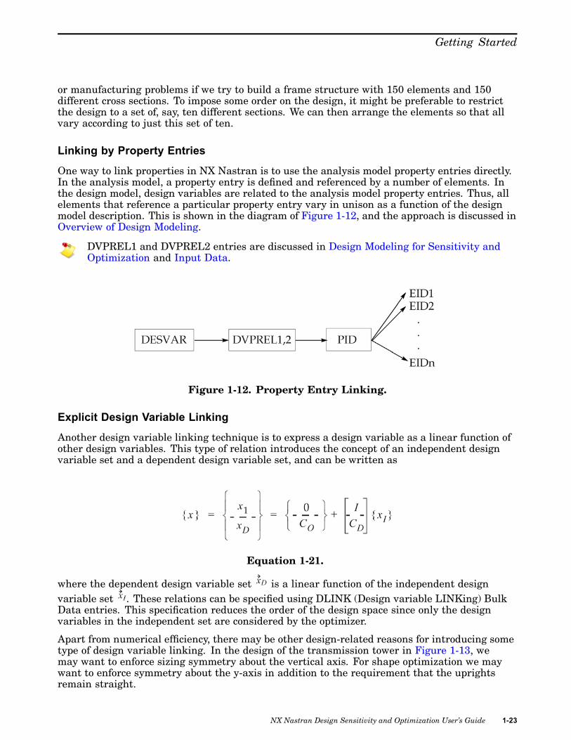
One way to link properties in NX Nastran is to use the analysis model property entries directly.In the analysis model, a property entry is defined and referenced by a number of elements. Inthe design model, design variables are related to the analysis model property entries. Thus, allelements that reference a particular property entry vary in unison as a function of the designmodel description. This is shown in the diagram of Figure 1-12, and the approach is discussed inOverview of Design Modeling.
DVPREL1 and DVPREL2 entries are discussed in Design Modeling for Sensitivity andOptimization and Input Data.
Figure 1-12. Property Entry Linking.
Explicit Design Variable Linking
Another design variable linking technique is to express a design variable as a linear function ofother design variables. This type of relation introduces the concept of an independent designvariable set and a dependent design variable set, and can be written as
Equation 1-21.
where the dependent design variable set is a linear function of the independent designvariable set . These relations can be specified using DLINK (Design variable LINKing) BulkData entries. This specification reduces the order of the design space since only the designvariables in the independent set are considered by the optimizer.
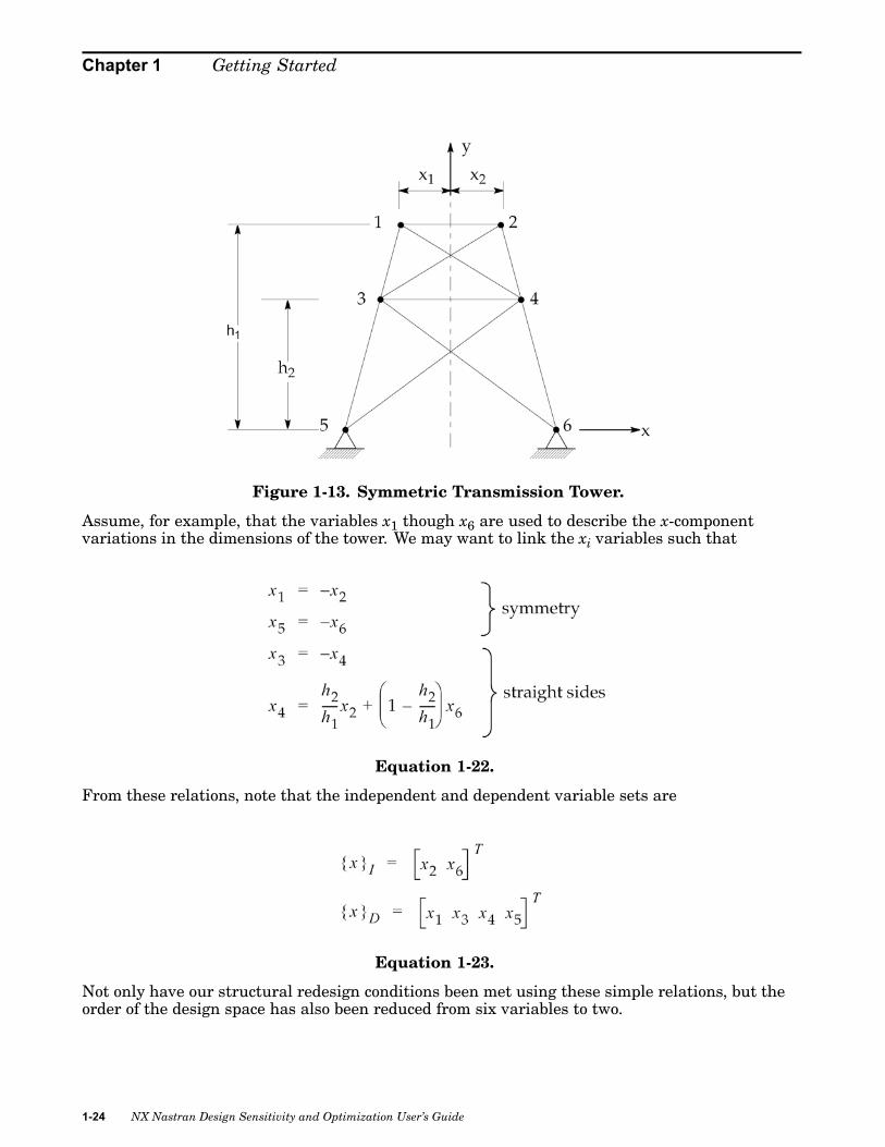
Apart from numerical efficiency, there may be other design-related reasons for introducing sometype of design variable linking. In the design of the transmission tower in Figure 1-13, wemay want to enforce sizing symmetry about the vertical axis. For shape optimization we maywant to enforce symmetry about the y-axis in addition to the requirement that the uprightsremain straight.
NX Nastran Design Sensitivity and Optimization User’s Guide 1-23
Chapter 1 Getting Started
Figure 1-13. Symmetric Transmission Tower.
Assume, for example, that the variables x1 though x6 are used to describe the x-componentvariations in the dimensions of the tower. We may want to link the xi variables such that
Equation 1-22.
From these relations, note that the independent and dependent variable sets are
Equation 1-23.
Not only have our structural redesign conditions been met using these simple relations, but theorder of the design space has also been reduced from six variables to two.
1-24 NX Nastran Design Sensitivity and Optimization User’s Guide

Getting Started
Constraint Regionalization and Deletion
If the number of constraints can be temporarily reduced, we would expect a reducedcomputational cost at both the numerical optimization level and, more importantly, at thesensitivity analysis level. This is because we reduce the number of structural responses forwhich gradient information must be computed.
Normalized Constraints in NX Nastran
In NX Nastran, constraints are internally generated in a normalized form, based on upperand lower response bounds selected by the engineer. Constraints may be present that dependon displacement, stress, eigenvalue responses, and so on. These response types may vary byorders of magnitude. To allow all constraints to be treated equally, regardless of the responsemagnitude, constraints in NX Nastran are normalized by the absolute values of the bounds. Theresult is that a constraint having a value of +1.0, for example, is violated by 100%, while aconstraint with a value of -0.5 is only 50% of its critical value (0.0). Upon scanning the valuesof all the normalized constraints, we may find that we only need consider a subset above aparticular threshold. Constraints below this value might then be temporarily disregarded onthe assumption that they are not currently driving the design.
This topic is discussed in Design Sensitivity and Optimization in NX Nastran in greaterdetail, but the general idea can be given here. Defining the Constraints discussesconstraint generation in NX Nastran in greater detail.
A negative value of a normalized constraint indicates constraint satisfaction, while apositive value indicates violation. See the Basic Optimization Problem Statement.
Figure 1-14 illustrates screening based on normalized constraints by representing the currentvalue of each constraint function in a bar chart format. If any constraint exceeds the “truncationthreshold” value denoted by TRS, we retain it for the ensuing approximate optimization, whiletemporarily deleting all others below TRS.
Constraint Screening
Figure 1-14. Constraint Deletion.
The default value for TRS is -0.5, but may be changed using the DSCREEN entry. SeeApproximation Concepts in Design Optimization for more details.
NX Nastran Design Sensitivity and Optimization User’s Guide 1-25

Chapter 1 Getting Started
If there are a large number of constraints below this truncation threshold (as is typical instructural optimization), the constraint screening phase will greatly simplify the optimizationtask. However, the number of constraints can still be further reduced using regionalization.
Constraint Regionalization
Suppose we have a particular section of an airplane wing skin, modeled with a numberof quadrilateral elements. This wing skin is to be of constant thickness for manufacturingconsiderations and is found to be overstressed in a number of locations. It would not makemuch sense to retain the stress constraints for every element in the skin panel since all of thesestresses will vary nearly in unison as the panel thickness is varied. The constraints from all ofthe neighboring elements will likely contain redundant information. Thus, it is probably safe toretain only a few of the largest valued constraints from this “region.”
Constraint regionalization is shown in Figure 1-16, which is the same as Figure 1-15, but withthe constraints grouped into three regions. For now, we will assume these regions have beenestablished based on some design model characteristics. Of the three regions shown, only twohave constraints that are numerically greater than the truncation threshold. These constraintswill pass the first screening test. Since the retained constraints within each region are likely tocontain redundant information, only the largest constraints from each region are retained. Theseconstraints are denoted by the check marks in the figure. NSTR, which in this example is 2,stands for the maximum number of constraints to be retained per region.
NSTR and TRS defaults can be overridden using the DSCREEN Bulk Data entry. Thenumber of regions are implicitly defined in connection with the DRESP1 Bulk Data entry.
Figure 1-15. Constraint Regionalization.
If NR is equal to the number of regions in our design model and NSTR is the maximum numberof constraints to be retained per region, then the maximum number of retained constraints isNR · NSTR. This is often one or two orders of magnitude less than the number of constraintsin the original set.
Formal Approximations
By applying constraint regionalization and deletion, we can reduce the number of constraints toonly that small subset that is necessary to adequately guide the design. However, we would still
1-26 NX Nastran Design Sensitivity and Optimization User’s Guide

Getting Started
like to replace the implicit and costly finite element analyses with explicit approximations for theobjective and constraint functions.
The approximating functions used in NX Nastran are based on Taylor series expansions of theobjective and constraints. For any function f(x) , an infinite series about a known value f(x0) interms of the change in the independent variable Δx can be written as
Equation 1-24.
In addition to the function value f(x0), this series requires that all derivatives atx0 be known aswell. Determining these derivatives may present some difficulty, so the series is often truncatedto a given power in Δx , yielding an approximate representation of the original function.
For example, if we only included through the first derivative term in the series, we would obtaina linear approximation:
Equation 1-25.
Since all terms of power Δx2 and higher have been omitted, the error in the approximation is onthe order of Δx2. This situation is shown in Figure 1-16, where the error increases with increasingvalues of |Δx|. Note that the approximation would be exact if the original function were linear.
Figure 1-16. Errors in Approximating Functions.
In design optimization, we are concerned not just with a single independent variable but ratherwith a vector of design variables, . Under this condition, the approximations for the objectiveand constraint functions become
NX Nastran Design Sensitivity and Optimization User’s Guide 1-27

Chapter 1 Getting Started
Equation 1-26.
where a gradient term replaces the first derivative term of Eq. 1-25.
We have not yet addressed the issue of how to determine the first derivative, or gradient,information. This information comes from the design sensitivity analysis. We introduce designsensitivity for linear static analysis here but reserve the discussion of the other analysisdisciplines for Design Modeling for Sensitivity and Optimization.
Many of our constraints, and perhaps the objective function as well, are based on responses thatdepend on the solution of the static equilibrium equations:
Equation 1-27.
For example, we may have an upper limit constraint on stress or
Equation 1-28.
The stress response σi is not only a function of the displacement solution {u} but also the elementgeometry and elastic properties, or
Equation 1-29.
where [D]B] is the stress-displacement transformation matrix. σj is a component of the elementstress vector {u}.
Partial differentiation of the stress constraint g with respect to the i-th design variable anduse of the chain rule for differentiation yields
Equation 1-30.
where ∂σj/∂xi is referred to as a sensitivity coefficient. In general, a sensitivity coefficient isdefined as the partial derivative of a response with respect to a design variable, or
1-28 NX Nastran Design Sensitivity and Optimization User’s Guide

Getting Started
Equation 1-31.
where rj is a general response quantity. Now,
Equation 1-32.
The first term of Eq. 1-32 is easily determined from relations such as Eq. 1-29. The secondterm can be evaluated if we first differentiate the static equilibrium equation (Eq. 1-27) withrespect to a design variable to obtain
Equation 1-33.
This relation can be solved for ∂{u } /∂xi to provide the information necessary to construct the firstorder approximations for the objective and retained constraints from Eq. 1-26. The solution ofEq. 1-33 is relatively inexpensive given that we already have the stiffness matrix [K ] availablein decomposed form as a result of static analysis.
A Simple Linear Design Space
At this point, it is probably worthwhile to take a look at a linearly approximated design spacejust to gain a qualitative understanding of the nature of the approximation. For this example, wecan again refer to the simple cantilever beam of Numerical Optimization Basics, Figure 1-6.
Recall that the design variables for the cantilever beam are the base B and height H of the beamcross section. If we construct linear approximations to the objective and constraint equationsaccording to Eq. 1-26, we have
NX Nastran Design Sensitivity and Optimization User’s Guide 1-29

Chapter 1 Getting Started
Equation 1-34.
For an initial design at (6,45), the derivatives in the above equation can be evaluated to yield
Equation 1-35.
The design space resulting from Eq.1-35 is shown in Figure1-17 superimposed on the true designspace. From the graph, note that the optimum resulting from this linear approximation happensto be at a slightly smaller value than the true objective. The linear approximation has allowedthe design to become slightly violated when compared to the true design space.
1-30 NX Nastran Design Sensitivity and Optimization User’s Guide

Getting Started
Figure 1-17. Linearly Approximated Cantilever Beam Design Space.
Though not yet an optimal design, the approximate optimum is a useful starting point for thenext approximate optimization cycle. This next cycle proceeds in exactly the same fashion; ananalysis is performed to determine the response values along with an evaluation of the responsederivatives. This information is then used to create another approximate subproblem thatshould, in turn, yield an even better approximation of the true optimum. After only a few morecycles, we may have reached a point sufficiently close to the true optimum that the processconverges as measured by the Kuhn-Tucker conditions.
Summary
By now you should have a fairly good idea of some of the various applications of designoptimization as well as some of the numerical optimization capabilities available to assist youin your design tasks. We introduced the basic ideas of numerical optimization and some of themethods that are used to couple it with structural analysis codes. Central to this has been therecognition that it is impractical to directly link numerical optimizers and structural analysiscodes to create a structural optimizer, and that some sort of approximations are required.
It has also been shown that the set of approximation concepts acts as an interface between theanalysis and the optimizer. There is really nothing extraordinary about these approximationssince in many ways they are similar to the methods experienced designers already use. Ofcourse, formalizing these methods in structural optimization allows problems of considerablygreater size and complexity to be solved than with traditional design methods alone.
NX Nastran Design Sensitivity and Optimization User’s Guide 1-31


Chapter
2 Design Modeling for Sensitivityand Optimization
• Overview of Design Modeling
• Defining the Analysis Disciplines
• Defining the Design Variables
• Relating Design Variables to Properties
• Relating Design Variables to Shape Changes
• Identifying the Design Responses
• Defining the Objective Function
• Defining the Constraints
• Superelement Design Modeling
NX Nastran Design Sensitivity and Optimization User’s Guide 2-1

Chapter 2 Design Modeling for Sensitivity and Optimization
A design model is required for design sensitivity and optimization in much the same way ananalysis model is required for finite element analysis. The design model is simply a formalstatement of allowable changes that can be made to a structure during the search for an optimaldesign. It also places limits on these allowable changes, and defines limits on the structuralresponses. Constructing the design model requires good engineering judgement if the designresults are to be of any practical use.
The essential features of the design model are that it must
• Define the design variables that may be modified.
• Describe the relationship between the design variables and the analysis model propertiesand/or grid locations (for shape optimal design).
• Define the objective function, which provides a scalar measure of design quality.
• Place bounds (constraints) limiting the design responses to an acceptable range.
This chapter describes each of these features in greater detail. In connection with this chapter,you may want to refer to Input Data, as well as Example Problems. These examples should all beavailable on your system. Running some of these in connection with the following discussions is agood way to begin to discover the many design modeling options available to you in NX Nastran.
2.1 Overview of Design ModelingGiven the wide range of problem types that may be addressed using design sensitivity andoptimization, the process of generating a design model is hardly a rote or mechanical operation.However, most of the operations are sufficiently similar that one might generate a flowchartoutlining the design modeling process as follows:
2-2 NX Nastran Design Sensitivity and Optimization User’s Guide

Design Modeling for Sensitivity and Optimization
Figure 2-1. Design Modeling Process.
The following sections discuss each of these items in greater detail. (Overriding optimizationcontrol parameters with the DOPTPRM and DSCREEN entries is reserved until afterapproximation concepts have been presented in Design Sensitivity and Optimization in NXNastran.)
2.2 Defining the Analysis DisciplinesA powerful feature of design sensitivity and optimization in NX Nastran is that you can specifythat a structure be subjected to a number of different analysis types for a number of various loadconditions. The optimizer will consider the results of all of these analyses simultaneously whenproposing an improved design. This approach is often described as multidisciplinary designoptimization, and is the only rational way of proposing a useful optimal design.
For example, you may have a component that is subjected to two static loading conditions. Thecomponent must also satisfy requirements on natural frequency bounds as determined from a
NX Nastran Design Sensitivity and Optimization User’s Guide 2-3

Chapter 2 Design Modeling for Sensitivity and Optimization
modal analysis. Further, the structure might also be subjected to transient loading conditionsfor which peak displacement responses might be of concern. We could quite easily introducethese different analysis types in Solution 200 (the solution sequence for design optimization)with the following input:
SOL 200cendspc = 100DESOBJ(MIN) = 15ANALYSIS = STATICSsubcase 1
DESSUB = 10displacement = allstress = allload = 1
subcase 2
DESSUB = 20displacement = allstrain(fiber) = allload = 2
subcase 3
ANALYSIS = MODESDESSUB = 30method = 3
subcase 4
ANALYSIS = MTRANDESSUB = 40method = 4dload = 4
begin bulk
Note some of the features in this example:
SOL 200 Executive command indicating Solution 200, the solution sequence fordesign sensitivity and optimization, is to be invoked.
ANALYSIS Case Control command indicating the analysis discipline to be used fora particular subcase (if appearing above a subcase level, all subsequentsubcases assume the same ANALYSIS command until changed). ANALYSISmay assume any of the following values:
STATICS StaticsMODES Normal ModesBUCK BucklingDFREQ Direct FrequencyMFREQ Modal FrequencyMTRAN Modal TransientSAERO Steady AeroelasticFLUTTER Flutter
DESOBJ Selects the design objective from a response defined in Bulk Data withDRESP1 or DRESP2.
2-4 NX Nastran Design Sensitivity and Optimization User’s Guide

Design Modeling for Sensitivity and Optimization
DESSUB Selects constraints to be applied at a particular subcase level from aDCONSTR set defined in Bulk Data.
DESOBJ and DESSUB are discussed in greater detail in Getting Started.
Case Control Output Requests in Design Optimization
In addition to the analysis-related Case Control commands, output requests might also appear,such as:
displacement= allstrain(fiber)= all
The frequency of data recovery output (e.g. first design cycle, last, every n-th, etc.) isgoverned by the Bulk Data parameter NASPRT. See Parameters for Design Sensitivityand Optimization for details.
These are of interest to design optimization in a couple of ways:
• In general, case control requests are for data recovery only; strictly speaking, they areunnecessary for design optimization. All necessary data recovery is automatically performedbased on the design responses identified in the Bulk Data (identifying the responses isdiscussed in Identifying the Design Responses. You do not need to explicitly request thisdata recovery unless you want to view the results.
• If various output forms are possible (e.g., strain(strcur) or strain(fiber)), design optimizationwill use the defaults unless a Case Control request to the contrary is provided. To use thepreceding example, STRAIN(STRCUR) representation is the default. If STRAIN(FIBER)is provided, data recovery and design optimization responses are both computed using thisform. Defaults are listed in the NX Nastran Quick Reference Guide.
Shape optimization and superelement optimization each have some additional Case Controlconsiderations beyond those related to data recovery. Superelement Design Modeling discussesthe Case Control structure for superelement design models. In addition, Example Problemsincludes examples of both shape and superelement optimization.
2.3 Defining the Design VariablesIn design optimization, design variables are the quantities that are modified by the optimizerduring the search for an improved design. In design sensitivity analysis, rates of change ofresponses are computed with respect to the design variables.
Defining the design variables is part of the design modeling task of the engineer. Once defined,the design variables may be used to
• Describe analysis model property variations.
• Define shape variations.
Design variables are often thought of as plate thicknesses, radii of cutouts, etc. Of course,design variables may be used to describe these quantities, but the idea is actually much moregeneral and powerful.
NX Nastran Design Sensitivity and Optimization User’s Guide 2-5
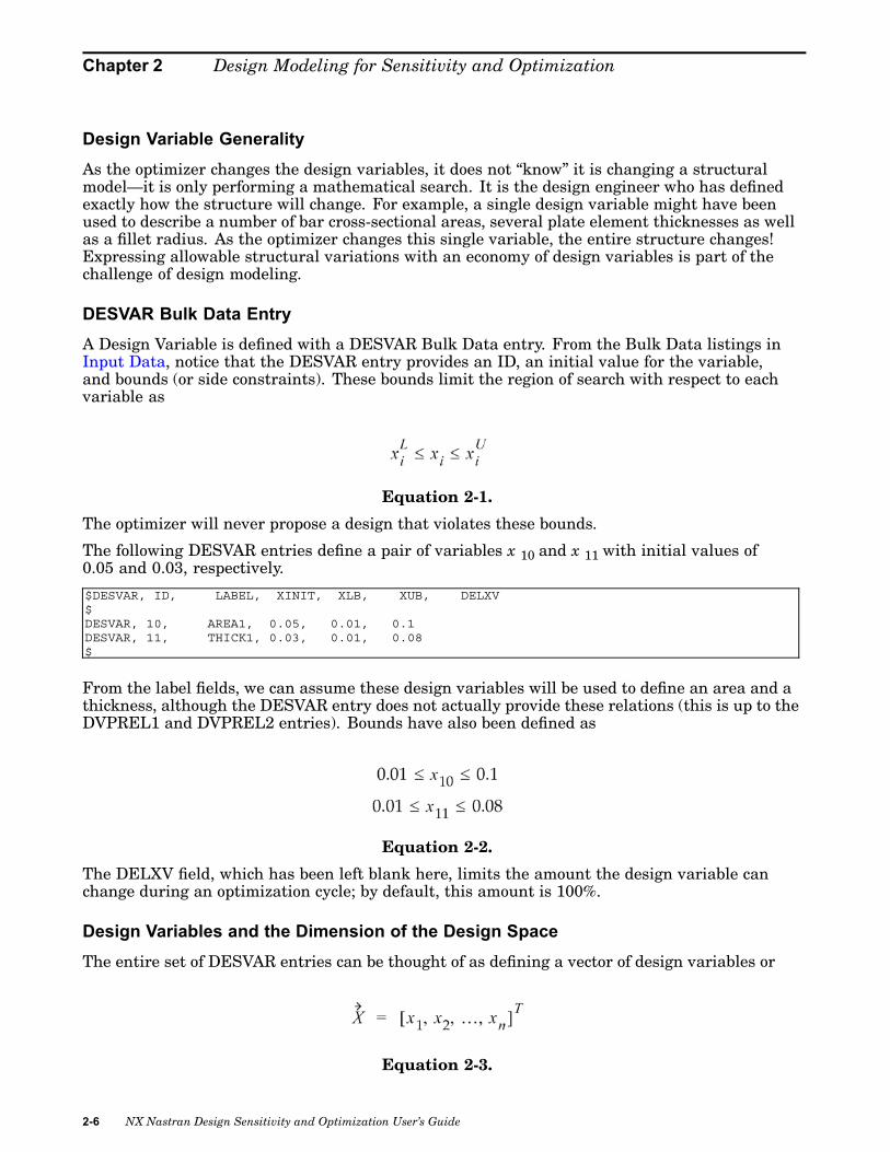
Chapter 2 Design Modeling for Sensitivity and Optimization
Design Variable GeneralityAs the optimizer changes the design variables, it does not “know” it is changing a structuralmodel—it is only performing a mathematical search. It is the design engineer who has definedexactly how the structure will change. For example, a single design variable might have beenused to describe a number of bar cross-sectional areas, several plate element thicknesses as wellas a fillet radius. As the optimizer changes this single variable, the entire structure changes!Expressing allowable structural variations with an economy of design variables is part of thechallenge of design modeling.
DESVAR Bulk Data EntryA Design Variable is defined with a DESVAR Bulk Data entry. From the Bulk Data listings inInput Data, notice that the DESVAR entry provides an ID, an initial value for the variable,and bounds (or side constraints). These bounds limit the region of search with respect to eachvariable as
Equation 2-1.
The optimizer will never propose a design that violates these bounds.
The following DESVAR entries define a pair of variables x 10 and x 11 with initial values of0.05 and 0.03, respectively.
$DESVAR, ID, LABEL, XINIT, XLB, XUB, DELXV$DESVAR, 10, AREA1, 0.05, 0.01, 0.1DESVAR, 11, THICK1, 0.03, 0.01, 0.08$
From the label fields, we can assume these design variables will be used to define an area and athickness, although the DESVAR entry does not actually provide these relations (this is up to theDVPREL1 and DVPREL2 entries). Bounds have also been defined as
Equation 2-2.
The DELXV field, which has been left blank here, limits the amount the design variable canchange during an optimization cycle; by default, this amount is 100%.
Design Variables and the Dimension of the Design SpaceThe entire set of DESVAR entries can be thought of as defining a vector of design variables or
Equation 2-3.
2-6 NX Nastran Design Sensitivity and Optimization User’s Guide

Design Modeling for Sensitivity and Optimization
To date, optimization problems with more than two hundred design variables have beenefficiently solved using NX Nastran.
The quantity n is often referred to as the dimension of the design space. The greater thedimension the more complicated the optimization task. The optimizer’s task is to find the bestconfiguration for these variables.
Design Variables and the Basic Optimization Problem StatementRecall that the problem we are trying to solve is defined by the basic optimization problemstatement, Eq. 2-1 through Eq. 2-5. Note that the design objective and constraint functions areexpressed as functions of design variables. How is this the case in structural optimization?
Assume that we are interested in minimizing the total structural mass for a particularmechanical component. This will be our objective function. We know that the mass is a functionof the properties used to describe the component as well as its shape. This can be expressed as
Equation 2-4.
where the vector is the collection of properties that describe the model and the vector is thecollection of grid point coordinates.
In the next sections, we will show how the properties and shape of the structure can be expressedas functions of design variables or
Equation 2-5.
By direct substitution of Eq. 2-5 into Eq. Eq. 2-4,
Equation 2-6.
or simply,
Equation 2-7.
To summarize, as the optimizer changes the design variables, the analysis model properties andshape will also change as defined by the design model. The modified properties and shape resultin changes to the computed responses that we have used to define the objective and constraintfunctions. Based on the modified objective and constraints, the optimizer can measure theamount of design improvement.
NX Nastran Design Sensitivity and Optimization User’s Guide 2-7

Chapter 2 Design Modeling for Sensitivity and Optimization
2.4 Relating Design Variables to PropertiesFor the analysis model to vary as the design variables are changed, its properties and/or itsshape must be expressed in terms of the design variables. You need to provide these relations aspart of the design model specification. This section discusses analysis model property changes.Relating Design Variables to Shape Changes discusses shape variations.
Definition of Analysis Model Properties
Analysis model properties are defined as those quantities that appear on Bulk Data propertyentries. Plate thicknesses, area moments of inertia, elastic spring stiffnesses, and so on, are allproperties that can be written as functions of design variables. Conversely, quantities such aselastic modulus, beam offset, or coefficients of thermal expansion cannot be functions of thedesign variables since they are not defined on property entries.
Type-1 Design Variable-to-Property Relations
You can relate design variables to analysis model properties in either of two ways: with linearrelations or with NX Nastran’s equation input capability. A linear relation is described using aDVPREL1 (Design Variable-to-Property RELation, type-1) Bulk Data entry.
Linear design variable-to-property relations are of the form
Equation 2-8.
where pj is the j-th property, expressed as a linear combination of i design variables.
Type-2 Design Variable-to-Property Relations
An equation, or type-2 relation, is defined using a DVPREL2 Bulk Data entry that references aDEQATN (Design EQuATioN) entry. A property expressed using these relations can be written as
Equation 2-9.
where the j-th property is a function of a collection of design variables and constants. Thefunction is defined using a DEQATN Bulk Data entry.
The same design variables may appear in either type-1 or type-2 relations. The block diagram ofFigure 2-2 may be helpful in understanding the role of the DVPREL1 and DVPREL2 entries indefining property variations.
2-8 NX Nastran Design Sensitivity and Optimization User’s Guide

Design Modeling for Sensitivity and Optimization
Figure 2-2. Design Variable-to-Property Relations.
The DVPREL1 entry defines linear property variations and requires only design variable input.All necessary constants are supplied directly on the entry. Thus, Figure 2-2 shows a single inputand a single output from the DVPREL1 block.
On the other hand, the DVPREL2 entry relies on an equation to describe the (generally)nonlinear property variations. This equation may have design variables (DESVAR) as well astable constants (DTABLE) as input. As shown in Figure 2-2, the result is again an analysismodel property variation.
Reference by Property Entry
In design variable-to-property relations, analysis model properties are referenced by propertyentry, rather than on an element-by-element basis. This relation is shown schematicallyin Figure 2-3. The property IDs PID1 through PIDm are referenced on the DVPREL1 andDVPREL2 entries. Since each of these property groups may contain a large number of elements(EID1 through EIDn), you can control many elements by using only a small set of DVPREL-typeentries. For example, to modify plate thicknesses, all that is required is to reference a PSHELLID on a DVPREL entry. All elements in the property group will then change accordingly.
Figure 2-3. Design Model Reference by Property Entry.
Identification of Property Entry Items
You must identify a selected property entry item either by its field position on the property BulkData entry or by its word position in the element property table (EPT) that is generated by NXNastran. In general, it is far easier to refer to the field position on the Bulk Data entry. In someinstances, (BEAM elements in particular) reference to the element property table must be made
NX Nastran Design Sensitivity and Optimization User’s Guide 2-9

Chapter 2 Design Modeling for Sensitivity and Optimization
instead. None of this is really as difficult as it sounds and is explained in the section on specialmodeling considerations at the end of this section.
To illustrate both type-1 and type-2 design variable-to-property relations, consider the stiffenedpanel section of Figure 2-4. The example is test problem library example number D200X7,presented in Stiffened Plate. Three design variables are each related to the plate thickness,web thickness, and cross-sectional area of the web cap, respectively. By grouping all of theelements in the base plate into one property group, their thickness can all be controlled by asingle design variable. This same grouping is also used for the elements of the web as well as forthe cap section elements.
Figure 2-4. Stiffened Panel Test Problem.
The base plate thickness is linearly related to a design variable according to
Equation 2-10.
This linear relation can be defined with a DVPREL1 Bulk Data entry as follows:
PSHELL, 1, 1, 0.15, 1$$...Define the design variables:$$DESVAR,ID, LABEL, XINIT, XLB, XUB, DELXVDESVAR, 1, T-PLATE,0.15, 0.001, 10.0$$...Relate the design variables to analysis model properties$ (linear relations, so use DVPREL1)$$DVPREL1,ID, TYPE, PID, FID, PMIN, PMAX, C0, , +$+, DVID1, COEF1, DVID2, COEF2, ...DVPREL1,1, PSHELL, 1, 4, 0.01, , , , +DP1+DP1, 1, 1.0
The PSHELL 1 entry defines the analysis model property group (to which a number of elementsbelong). The DESVAR 1 entry defines design variable 1 (T-PLATE) with an initial value of 0.15
2-10 NX Nastran Design Sensitivity and Optimization User’s Guide

Design Modeling for Sensitivity and Optimization
and lower and upper bounds of .001 and 10.0, respectively. Design variable 1 is, in turn, relatedto PSHELL property group 1 thickness via DVPREL1 number 1. The 4 in DVPREL1 number1, field 5, states that it is field 4 on the property entry (the thickness) that is to be varied. Thecontinuation line on the DVPREL1 entry gives the functional relationship defined by Eq. 2-10.Field 6 on the DVPREL1 entry defines the minimum allowable value of the property; here, aminimum thickness of 0.01. This value enforces a lower bound, even though greater than thedesign variable’s lower bound. See Stiffened Plate for the remainder of the design model.
Frequently, you may want to specify the bar cross-sectional dimensions in the design modelinstead and use this data to compute the resultant cross-sectional properties, such as areas andmoments of inertia. Since these properties are often nonlinear functions of the design variables,this approach requires the use of type-2 design variable to property relations. Probably theeasiest way to introduce type-2 relations is with a simple example:
Figure 2-5. Cap Section Detail.
Assume that the cap section of the stiffened plate of Figure 2-4 is a rectangular section bar asshown in Figure 2-5. Suppose the bar is characterized by the cross-sectional dimensions b and hand is oriented with respect to principal planes 1 and 2 as shown. A stress recovery location,such as point c, might be defined as well. The Bulk Data describing the analysis and designmodel relations could be written as follows:
$...ANALYSIS MODEL PROPERTIES:PBAR, 120, 220, 0.12, 9.0E-4, 1.6E-3, , , , ++, -.15, .2$$...BAR CROSS-SECTIONAL DIMENSIONS:$ESVAR, ID, LABEL, XINIT, XLB, XUB, DELXVDESVAR, 10, B, .3, .1, 1.0DESVAR, 11, H, .4, .1, 1.0$$...BAR PROPERTY RELATIONS, A, I1, I2:$DVPREL2,ID, TYPE, PID, FID, PMIN, PMAX, EQID, , +$+, DESVAR,DVID1, DVID2, ..., , , , , +$+, DTABLE,CID1, CID2, ...DVPREL2,250, PBAR, 120, 4, , , 501, , ++, DESVAR, 10, 11DVPREL2,251, PBAR, 120, 5, 1.0E-5 , 502, , ++, DESVAR, 10, 11DVPREL2,252, PBAR, 120, 6, 1.0E-5 , 503, , ++, DESVAR, 10, 11$$...EQUATIONS:DEQATN 501 AREA(B,H) = B*HDEQATN 502 I1(B,H) = H*B**3/12.DEQATN 503 I2(B,H) = B*H**3/12.
NX Nastran Design Sensitivity and Optimization User’s Guide 2-11

Chapter 2 Design Modeling for Sensitivity and Optimization
$$...STRESS RECOVERY POINT LOCATIONS:$DVPREL1,ID, TYPE, PID, FID, PMIN, PMAX, C0, , +$+, DVID1, COEF1, DVID2, COEF2, ...DVPREL1,260, PBAR, 120, 12, -.5 , , , ++, 10, -.5DVPREL1,261, PBAR, 120, 13, .05, , , , ++, 11, .5
PBAR 120 defines the bar properties corresponding to the initial cross-sectional dimensions.Note that the initial values of the design variables listed on the DESVAR entries agree with theinitial properties. If any discrepancies exist between the initial analysis model properties (givenon the property entries) and those calculated based on the initial values of the design variables,the properties based on the design model have precedence. The design model data is then used tooverride the analysis model properties. In this example, the design and analysis model agree,and no overrides take place.
Since the bar area and moments of inertia are nonlinear in the design variables, they must bedefined using equations. These relations are defined on the DEQATN entries 501, 502, and 503.The input arguments are assigned via the DVPREL2 entries 250, 251, and 252. The DESVARidentifier on the first continuation of each of these entries indicates design variables 10 and 11are to be used as input (b and h) for each of the referenced equations.
Override of analysis model data by design model data provides a convenient methodof restarting in design optimization. See the restart example in Restarts in DesignOptimization.
Equation ArgumentsThe input arguments defined on the DEQATN entries are formal arguments, which are definedat run time by the actual arguments provided on the DVPREL2 entries. The rules for definingthese equations follow directly from FORTRAN syntax requirements. However, all argumentsare assumed to be real numbers. FORTRAN intrinsic functions may also be used. (Some of thesefunctions, such as ABS and MAX, are not recommended since they may yield functions havingdiscontinuous first derivatives. The sensitivity analysis as well as the optimization results maybe incorrect if any of these discontinuities are encountered.)
The available intrinsic functions and their uses are listed with the DEQATN bulk dataentry in the NX Nastran Quick Reference Guide.
Minimum Allowable Property ValuesField 6 on the DVPREL2 entries define PMIN, which is the minimum allowable value for theparticular property during design optimization. Generally, its purpose is to prevent propertiesfrom taking on values near zero. The default is 0.001, which is acceptable for many applications.Here, the initial value of I1 is less than this default minimum; therefore, PMIN is specified as1.0E-5 on DVPREL2 251. Since I2 might also assume values on this order of magnitude, itsPMIN is overridden as well.
PMAX has been added to the DVPREL1 and DVPREL2 entries. See Input Data.
A similar situation is seen in the DVPREL1 relations that in this case, relate the location ofthe stress recovery point c to the values of the design variables. The y-coordinate location isa negative quantity, but the default PMIN for stress recovery locations is -1.0E+35 (see theDVPREL1 and DVPREL2 Bulk Data entry descriptions). Just to be explicit, a negative PMIN
2-12 NX Nastran Design Sensitivity and Optimization User’s Guide

Design Modeling for Sensitivity and Optimization
has been provided on DVPREL1 260. DVPREL1 260 and 261 respectively, define the followinglinear relations:
Equation 2-11.
Stress Recovery Locations: Words of Warning
Note the error that may have resulted if the location of the stress recovery point had not beenallowed to vary. Since the stress computations would not have included the direct effects ofchanges in the stress recovery point, the stresses seen by the optimizer would not be thosethat the engineer had intended. This would certainly lead to incorrect results. Of course,other stress recovery points would probably also need to be defined to ensure recovery of themaximum stresses.
Special Design Modeling Considerations - BEAM Elements
In design modeling, the BEAM element differs from other element types in that its propertiesmust be referenced according to their word positions in the element property tables. The elementproperty tables are internally generated in NX Nastran, and used to form the element-levelstructural matrices.
By convention, field position identifiers are denoted as positive quantities on DVPRELientries, EPT word positions as negative quantities.
The source of this difference is due to the generality of the PBEAM Bulk Data entry. Since asingle entry can used to specify the BEAM’s cross-sectional properties for both ends and up tonine intermediate stations, a unique correspondence between a BEAM property and its fieldposition on the PBEAM entry is not assured. The only relation that is assured is the one betweena property item and its word position in the element property table. This correspondencerequires that the engineer have some understanding of the structure of the EPT for the BEAMelement and its relation to the data supplied on the PBEAM entry.
Note that the numbering in Figure 2-6 is offset by a value of 1 from that given in the NXNastran Reference Manual, Section 15.9. Figure 2-6 applies to the “new” design sensitivityand optimization (Solution 200), while the figure in the NX Nastran User’s Manual appliesto the “old” DSA Solution Sequences, 51, 53, and 55 (and 101, 103, and 105).
In general, the cross section of a BEAM element may be either constant, linear, or variable.These three possibilities are shown in Figure 2-6, which is a schematic of the EPT configurationfor each of these situations.
NX Nastran Design Sensitivity and Optimization User’s Guide 2-13

Chapter 2 Design Modeling for Sensitivity and Optimization
2-14 NX Nastran Design Sensitivity and Optimization User’s Guide

Design Modeling for Sensitivity and Optimization
Figure 2-6. Element Property Table for BEAM Element.
Item 1 in Figure 2-6 is a diagram of the EPT for the BEAM element when the PBEAM entryfurnishes data at end A only. End B data is built internally as a copy of end A properties. Sincethis structure is used by subsequent modules to generate the element mass and stiffnessmatrices, the design model must also define equal variations for both sets of data. Thus, fordesign sensitivity and optimization, you must prescribe EPT word positions 166-181 (end B) inaddition to words 6-21 (end A). Otherwise, the ensuing incompatibility between end A and end Bdata will invalidate the subsequent analysis results.
Item 2 in Figure 2-6 shows the structure of the EPT for a tapered beam. The data for ends A andB is determined based on the supplied PBEAM input. Additionally, the first intermediate station(Words 22-37) is internally generated and contains a copy of end B data. Your design model mustthen reference words 6-21 for end A, words 166-181 for end B, and the first intermediate station.
The most general case is shown in item 3 where, in addition to ends A and B, from one to nineintermediate stations are defined. As in item 2, the first available intermediate station alwayscontains a copy of end B data. This must always be accounted for in the design model definition.(Note that if nine intermediate stations are defined, there is no need to supply an additional copyof end B data since the next station is end B itself.)
To illustrate, consider the uniformly tapered beam element in Figure 2-7. The cross-sectionaldimensions for a rectangular element can be described in terms of design variables b 1 , h 1 , b 2 ,and h 2 as shown in the figure. An input data file using this element in a single-element designsensitivity test is given in Listing 2-1. This example corresponds to a test of Item 2 in Figure 2-6.
NX Nastran Design Sensitivity and Optimization User’s Guide 2-15

Chapter 2 Design Modeling for Sensitivity and Optimization
Figure 2-7. Tapered Rectangular Beam Element.
The initial design is given by
Equation 2-12.
This design is input to the DEQATN entries to define the corresponding cross-sectionalproperties for the element.
In addition to the properties at ends A and B, the design model must also include a definitionfor the first intermediate station. The properties at end A are expressed as functions of DesignVariables 1 and 2 via DVPREL2s 1-5, end B properties are expressed in terms of DesignVariables 3 and 4 via DVPREL2s 6-10, and the first intermediate station by DVPREL2s 11-15.
In order to make identification of the EPT word positions easier, the PBEAM entry has been setup to define cross-sectional properties that are slightly different from the properties computedusing the initial design variable values. The design model overrides the analysis model propertiesand the differences reported in a differences comparison table. Since the word positions in theEPT are also output, these results can be used to check the validity of the formulation.
The design model should include stress recovery point locations. Serious design errorsmay result if you omit these from your design model formulation.
The difference comparison table associated with the design model override is shown in Figure2-8. From the corresponding field IDs (FID) it can be seen that not only is the data for ends A
2-16 NX Nastran Design Sensitivity and Optimization User’s Guide

Design Modeling for Sensitivity and Optimization
and B in the expected word positions, but the intermediate station is also present as expected.The analysis and design property columns indicate that it is indeed just a copy of the datafor end B. Furthermore, the design model formulation appears to be correct judging from thenumber, location, and values of the design model override data.
Figure 2-8. Message Indicating an Analysis Model Override by the Design Model.
$>>>>>>>>>>>>>>>>>>>>>>>>>>>>>>>>>>>>>>>>>>>>>>>>>>>>>>>>>>>>>>>>>>>>>>>>>>>>>>>$ BEAM MODELING TEST, VERSION 2$$ TAPERED BEAM WITH RECTANGULAR SECTION, DESIGN SENSITIVITY ANALYSIS. SINCE$ BOTH ENDS A AND B ARE SPECIFIED ON THE PBEAM ENTRY, DESIGN CHANGES MUST$ BE SPECIFIED NOT ONLY FOR THE ENDS, BUT ALSO FOR THE FIRST INTERMEDIATE$ STATION, WHICH CONTAINS A COPY OF END B DATA.$$$ PLANE 2$ |$ ----*----$ | |$ H | | --- PLANE 1$ | |$ ----*----$ B * = STRESS RECOVERY LOCATIONS$$$>>>>>>>>>>>>>>>>>>>>>>>>>>>>>>>>>>>>>>>>>>>>>>>>>>>>>>>>>>>>>>>>>>>>>>>>>>>>>>>$TIME 10SOL 200CEND$$ CC FOR ANALYSIS:DISP = ALLSTRESS = ALL
NX Nastran Design Sensitivity and Optimization User’s Guide 2-17

Chapter 2 Design Modeling for Sensitivity and Optimization
SPC = 100LOAD = 300$ CC FOR OPTIMIZATION:ANALYSIS = STATICSDESOBJ(MIN) = 8 $ OBJECTIVE FUNCTION DEFINITIONDESSUB = 10 $ CONSTRAINT SET SELECTION$BEGIN BULK$PARAM, OPTIM, NOPARAM, OPTEXIT, 4$-------------------------------------------------------------------------------$ ANALYSIS MODEL$-------------------------------------------------------------------------------MAT1 110 10.0E6 0.33 0.1 +M1+M1 50000. 50000. 29000.GRDSET 4GRID 1 0.0 0.0 0.0GRID 2 20. 0.0 0.0CBEAM 1 100 1 2 0.0 1.0 0.0$$ PBEAM ENTRY INPUT WITH SLIGHT ‘ERROR’ IN TERMS. THIS HELPS VALIDATE THE DE-$ SIGN MODEL BECAUSE USER WARNING MESSAGE WILL BE ISSUED, CONFIRMING OVERRIDE.$PBEAM 100 110 2.01 .167 .667 +P11+P11 0.0 1.01 0.0 -1.01 +P12+P12 YES 1.0 0.51 .0104 .042 +P13+P13 0.0 0.51 0.0 -0.51$SPC1 100 123456 1FORCE 300 2 20000.0 0.0 0.0 -1.0$-------------------------------------------------------------------------------$ DESIGN MODEL$-------------------------------------------------------------------------------$$...END A DATA: (A,I1,I2,C2,D2)$$DESVAR,ID, LABEL, XINIT, XLB, XUB, DELXVDESVAR, 1, B1, 1.0, 0.1, 10.0DESVAR, 2, H1, 2.0, 0.2, 20.0
$$DVPREL2,ID, TYPE, PID, FID, PMIN, PMAX, EQID, , +$+, DESVAR, DVID1, DVID2, ..., , , , , +$+, DTABLE, CID1, CID2, ...DVPREL2,1, PBEAM, 100, -8, , , 101, , ++, DESVAR, 1, 2DVPREL2,2, PBEAM, 100, -9, , , 102, , ++, DESVAR, 1, 2DVPREL2,3, PBEAM, 100, -10, , , 103, , ++, DESVAR, 1, 2DVPREL2,4, PBEAM, 100, -15, , , 104, , ++, DESVAR, 2DVPREL2,5, PBEAM, 100, -17, , , 105, , ++, DESVAR, 2$$...END B DATA: (A,I1,I2,C2,D2)$$DESVAR,ID, LABEL, XINIT, XLB, XUB, DELXVDESVAR, 3, B2, 0.5, 0.05, 10.0DESVAR, 4, H2, 1.0, 0.1, 20.0$$DVPREL2,ID, TYPE, PID, FID, PMIN, PMAX, EQID, , +$+, DESVAR, DVID1, DVID2, ..., , , , , +$+, DTABLE, CID1, CID2, ...DVPREL2,6, PBEAM, 100, -168, , , 101, , ++, DESVAR, 3, 4
2-18 NX Nastran Design Sensitivity and Optimization User’s Guide

Design Modeling for Sensitivity and Optimization
DVPREL2,7, PBEAM, 100, -169, , , 102, , ++, DESVAR, 3, 4DVPREL2,8, PBEAM, 100, -170, , , 103, , ++, DESVAR, 3, 4DVPREL2,9, PBEAM, 100, -175, , , 104, , ++, DESVAR, 4DVPREL2,10, PBEAM, 100, -177, , , 105, , ++, DESVAR, 4$$...FIRST INTERMEDIATE STATION (COPY OF END B DATA): (A,I1,I2,C2,D2)$$DVPREL2,ID, TYPE, PID, FID, PMIN, PMAX, EQID, , +$+, DESVAR, DVID1, DVID2, ..., , , , , +$+, DTABLE, CID1, CID2, ...DVPREL2,11, PBEAM, 100, -24, , , 101, , ++, DESVAR, 3, 4DVPREL2,12, PBEAM, 100, -25, , , 102, , ++, DESVAR, 3, 4DVPREL2,13, PBEAM, 100, -26, , , 103, , ++, DESVAR, 3, 4DVPREL2,14, PBEAM, 100, -31, , , 104, , ++, DESVAR, 4DVPREL2,15, PBEAM, 100, -33, , , 105, , ++, DESVAR, 4$DEQATN 101 AREA(B,H) = B*HDEQATN 102 I1(B,H) = H*B**3/12.DEQATN 103 I2(B,H) = B*H**3/12.DEQATN 104 C2(H) = H/2.DEQATN 105 D2(H) = -H/2.$$DRESP1,ID, LABEL, RTYPE, PTYPE, REGION, ATTA, ATTB, ATT1, +$+, ATT2, ...DRESP1, 7, D2, DISP, , , 3, , 2DRESP1, 8, W, WEIGHT$$DCONSTR,DCID, RID, LALLOW, UALLOWDCONSTR, 10, 7, -3.0, 3.0$$.......2.......3.......4.......5.......6.......7.......8.......9.......0ENDDATA
Listing 2-1.
2.5 Relating Design Variables to Shape ChangesTo use shape sensitivity and optimization in NX Nastran, you must define design variables, andrelate them to allowable shape variations. The amount the design variable is changed duringoptimization results in a corresponding shape change.
The allowable shapes are defined using shape basis vectors. The engineer uses these to describehow the structure is allowed to change. The optimizer then determines how much the structurecan change by modifying the design variables. There are four methods are available to describethese shape basis vectors:
• Manual grid variation.
• Direct input of shapes.
• Geometric boundary shapes.
NX Nastran Design Sensitivity and Optimization User’s Guide 2-19

Chapter 2 Design Modeling for Sensitivity and Optimization
• Analytic boundary shapes.
This section begins with a brief theoretical discussion of shape basis vectors, followed by anintroduction to auxiliary models, which you can use in NX Nastran as an aid to shape basis vectorgeneration. Following these discussions is an overview of the various modeling methods availableas well as an example highlighting some of the differences among these various approaches.
Other examples can be found in Example Problems, Example Problems. Interested readers mayalso refer to Design Sensitivity and Optimization in NX Nastran for details regarding shapesensitivity analysis.
Basis Vectors in Shape Optimization
Shape basis vectors are used in NX Nastran to describe the properties of characteristic, allowableshape changes. The optimizer then determines the best linear combination of these vectors,given the design criteria established by the engineer.
Although the mathematics of shape basis vectors are quite simple, it is probably best to introducethe idea with a simple example.
The simple angle bracket redesign of Figure 2-9 can be used to illustrate the properties ofshape basis vectors.
Figure 2-9. Angle Bracket
Suppose the design goal is to vary the lengths of the x- and y-axis legs of the bracket whilekeeping the outer edge straight. The location of all grid points along this edge can easily bedescribed in terms of the bracket leg lengths. For simplicity, assuming only four grids alongthis edge, we can write
Equation 2-13.
2-20 NX Nastran Design Sensitivity and Optimization User’s Guide

Design Modeling for Sensitivity and Optimization
A more realistic model certainly would include more grid points along this edge in addition to anumber of grids in the structure’s interior. Adding these grids would simply add more equationsto the set in Eq. 2-13, leaving its basic form unchanged.
We can write Eq. 2-13 in terms of grid variations as
Equation 2-14.
The coefficient matrix is unchanged in Eq. 2-14 from that of Eq. 2-13.
Eq. 2-14 suggests that a convenient choice of design variables would be
Equation 2-15.
Equation 2-16.
Note that Eq. 2-16 expresses a vector of grid coordinate changes in terms of a vector of designvariable changes. Each column of the matrix on the right-hand side of the equation is called ashape basis vector. Generating the shape basis vectors is one of the design engineer’s primarytasks in shape optimization.
If we graph each column of the matrix in Eq. 2-16 as a set of grid displacements, we see thatcolumn 1 represents a vertical (or y-component) variation in shape, while column 2 represents ahorizontal shape variation. (The column order is arbitrary and just depends on the order of thedesign variables.) Note that both shape basis vectors, as well as any linear combination of them,keep the edge of the bracket as a straight line, consistent with our design goals.
NX Nastran Design Sensitivity and Optimization User’s Guide 2-21

Chapter 2 Design Modeling for Sensitivity and Optimization
Figure 2-10. Basis Vectors for the Angle Bracket.
Once a shape basis vector description is available, the optimizer can vary the shape of thestructure by changing the corresponding design variables.
Reduced Basis Formulations
We can generalize the relation given in Eq. 2-16 as
Equation 2-17.
where:
Equation 2-18.
and i = design cycle number.
Eq. 2-17 expresses a vector of grid point changes as a function of changes in design variables.The linear combination of design variable changes times each shape basis vector results in thetotal change in shape. Typically, there are more grid points than design variables, or m » n. Forthis reason, Eq. 2-17 is often called a reduced basis formulation.
Auxiliary Models in Shape Optimization
An auxiliary model is simply an additional finite element model used to generate shape basisvectors. Rather than tediously specifying shape changes on an individual grid-by-grid basis,auxiliary models are a tool that can be used to simplify this process. An auxiliary model usuallyshares the same geometry, element connectivity, and (possibly) material type as the originalstructure. However, boundary conditions usually differ. Applying loads to this structure willresult in sets of displacement vectors {U}. When we think of these displacement components
2-22 NX Nastran Design Sensitivity and Optimization User’s Guide

Design Modeling for Sensitivity and Optimization
as representing individual components of grid motion, we realize that the {U } vectors can bequite conveniently used as basis vectors for shape optimization.
For example, consider the cantilever beam of Figure 2-11. The analysis model is clamped alongthe left-hand edge and tip-loaded on the right. Suppose we would like to redesign the shape ofthe structure by modifying the profile of the lower edge. In order to do so, we might like to use anauxiliary model to generate a few characteristic profiles and use these as our shape basis vectors.
Figure 2-11. Simple 2-D Cantilever.
Figure 2-12 shows the corresponding auxiliary model and its boundary conditions, exclusive ofthe loading. The fixed edges A and B guarantee that the left-hand support and the horizontalupper edge will not change during shape optimization. The roller supports along edge C willallow the depth of the beam to change without changing its length. We can now load edge D anyway we want to produce a range of “shapes” or basis vectors.
Figure 2-12. Auxiliary Model for the Simple 2-D Cantilever.
A uniform taper component might be generated by applying SPCDs as shown in Figure 2-13.Here, the displacements have been plotted to show the basis vector characteristics. Visualizationof these basis vectors prior to their use in connection with shape optimization is highlyrecommended. (An alternate approach might be to add some very stiff beams to the bottom edgeof the auxiliary model. Loading the tip of the rightmost beam would then approximate the effectof the SPCD’s used here.)
NX Nastran Design Sensitivity and Optimization User’s Guide 2-23

Chapter 2 Design Modeling for Sensitivity and Optimization
Figure 2-13. Uniform Taper Basis Vector.
A more arbitrary shape basis vector could be generated by loading one of the individual gridsalong the lower edge. The produces an indent as shown in Figure 2-14. A number of theseshapes produced by loading other grids along this edge might comprise a useful set of shapebasis vectors, depending on the desired effect.
Figure 2-14. Point-Load Basis Vector.
Modeling Methods (Shape Basis Vector Definition)
Basic AssumptionsShape optimization in NX Nastran assumes the engineer is starting with a reasonably gooddesign but would like to investigate ways in which the shape of the part, or even the entirestructure, might be modified in order to better meet the design goals.
Although large shape variations can be investigated in NX Nastran, it is important to notethat in a practical design environment, shape changes are often limited by numerous designconsiderations. Manufacturability of the part, interference from neighboring components of thestructure, aesthetics, and so on, often limit the degree to which the structural shape can bemodified.
Shape optimization in NX Nastran allows you to investigate these “real world” types of shapevariations. It will, for example, let you determine the optimum placement and size of cutouts tolighten a structure. What the code will not tell you is how many of these cutouts to start withor whether an alternate method of construction is better. In fact, the latter questions are stillactive areas of shape optimization research.
Goal of Design Modeling for ShapeFour different modeling methods are available in NX Nastran. The purpose of each methodis the same—to define a basis vector (or a set of basis vectors) for shape optimization. Themethods only differ in terms of their user interfaces and whether or not the basis vectors are
2-24 NX Nastran Design Sensitivity and Optimization User’s Guide

Design Modeling for Sensitivity and Optimization
automatically updated on each design cycle. The following subsections briefly outline eachapproach, its strong as well as its possible weak points, and its requirements for use.
Manual Grid Variation
This is the most general, as well as perhaps the most tedious, method of generating Shapebasis vectors. It is listed first since it can be thought of as the lowest level approach, somewhatanalgous to Assembly Language versus FORTRAN programming. A DVGRID Bulk Data entrydefines the direction and magnitude of a grid variation for a given change in a design variable.This relation is shown in Figure 2-15 and Eq. 2-19. A single DVGRID entry is required forevery design variable-grid pair. (See Commonly Used Commands for Design Optimization forthe DVGRID entry format.)
Figure 2-15. Grid Point Variation Defined by a DVGRID Entry.
Equation 2-19.
DVGRID entries alone can be used to describe shape changes, although the method is probablymore useful when combined with the direct input of shapes approach. Its most powerful form,however, is in connection with the geometric shapes approach. (These methods are describedlater in this section.)
Benefits
Since this can be considered the lowest-level approach, its strength lies in its generality. UsingDVGRIDs alone, the designer has direct control over every designed grid point in the model (thatis, every grid point whose location is to change during shape optimization.)
NX Nastran Design Sensitivity and Optimization User’s Guide 2-25

Chapter 2 Design Modeling for Sensitivity and Optimization
DrawbacksIn all but the simplest of problems, the data input can be formidable without a preprocessor.The resultant basis vectors are treated as constant and not updated with each design cycle,so the risks of mesh distortion are increased.
Checklist1. Define the shape design variables using DESVAR Bulk Data entries.
2. Establish the corresponding grid variations using DVGRID Bulk Data entries, one entryfor every design variable-designed grid pair in the model. This entry ties design variablechanges to changes in the structure’s shape. (Of course, this may lead to a large amount ofdata, up to G*NDV where G is the number of designed grids in the model and NDV is thenumber of shape design variables. A model with only 100 grids and 2 design variables wouldthus require on the order of 200 DVGRID entries.)
3. Preview the resultant basis vectors, and modify if necessary.
Direct Input of ShapesThis approach greatly simplifies the process of defining shape basis vectors. With this method,externally-generated vectors are DBLOCATEd and used to define shape basis vectors. Anauxiliary model analysis provides these externally-generated vectors.
BenefitsBasis vectors for shape optimization can be generated using an external auxiliary model analysisand DBLOCATEd, allowing for easy generation of shape basis vectors. In theory, any methodof external generation is possible, as long as the number of degrees of freedom in the auxiliarymodel is the same as in the primary structure (i.e., G-sets must be equivalent).
DrawbacksThe process is not fully automatic since an auxiliary model analysis must be performedbeforehand, saved on the database, and DBLOCATEd for shape optimization. Since the basisvectors are externally generated, they are not updated for each design cycle. This may causemesh distortion problems for large shape changes.
Checklist1. Define an auxiliary model, perform an analysis, and save the results to the database using
the SCR=NO option on the NASTRAN job submittal command. This process is the same as aconventional NX Nastran analysis except that the auxiliary model geometry and boundaryconditions have been established with consideration given to the shape redesign goals.
2. DBLOCATE the results for shape optimization using the following FMS section commands(assuming the master file is file1.MASTER):
ASSIGN FILE1 = “file1.MASTER”DBLOCATE DATABLK=(UG/UGD,GEOM1/GEOM1D,GEOM2/GEOM2D),LOGICAL=FILE1
Note: The data blocks UG, GEOM1, and GEOM2, are DBLOCATEd and renamed to UGD,GEOM1D, and GEOM2D, respectively. The data block names UGD, GEOM1D, and GEOM2Dcannot be changed.
2-26 NX Nastran Design Sensitivity and Optimization User’s Guide

Design Modeling for Sensitivity and Optimization
3. Define shape design variables using DESVAR entries, and correlate these to theDBLOCATEd basis vectors using DVSHAP Bulk Data entries.
4. Preview the resultant shape basis vectors to check for modeling errors.
Geometric Boundary Shapes
This method defines allowable shape variations using only the boundary of the structure. Theseshape variations can be supplied manually or with a geometry-based preprocessor. Eitherapproach relies on BNDGRD Bulk Data entries to define the structure’s boundaries and DVGRIDentries to furnish the shape variations over these boundaries.
Shape basis vectors are automatically generated by the code through a process of interpolation ofthe boundary shape changes to the interior of the structure. Additionally, the shape basis vectorsare updated on every design cycle, minimizing the problems associated with mesh distortion forlarge shape changes.
Benefits
Since grid variations need only be specified over the boundaries, data preparation is greatlysimplified. In fact, since DVGRID entries are only written for the boundaries, many real-worldproblems can be effectively solved without geometry-based preprocessors. Internal computationof the shape basis vectors means that these can be recomputed (updated) for every design cycle,reducing the problems associated with mesh distortion for large shape changes.
Drawbacks
Describing grid variations over the boundaries may still require a lot of DVGRID information,even though orders of magnitude less than the manual grid variation method.
Checklist
1. Define the shape design variables using DESVAR Bulk Data entries.
2. Define corresponding shape variations over the structure’s boundaries using DVGRIDentries.
3. Define the shape boundary conditions using BNDGRID Bulk Data entries. TheBNDGRID-DVGRID entry combination is analogous to the use of SPCDs to impose enforcedboundary displacements. The DVGRID entry supplies the enforced variation, much like anSPCD, to the boundary grids specified on the BNDGRID entry (similar to an SPC entry).
Analytic Boundary Shapes
This approach is similar to the geometric boundary shapes method but avoids having to useDVGRID entries on the boundary. Instead, the designer provides an auxiliary model overthe boundaries of the structure that are to be changed. This may be a collection of BARelements along the edges of a two-dimensional structure or a “skin” of plate elements overa three-dimensional part. We often refer to this model over the boundaries as an auxiliaryboundary model. The designer then constrains and statically loads the model to produce a shapevariation over the boundary, which the code then interpolates to the interior of the structure.The result is a shape basis vector for optimization.
NX Nastran Design Sensitivity and Optimization User’s Guide 2-27

Chapter 2 Design Modeling for Sensitivity and Optimization
Benefits
The method is very general, and does not require a geometry-based pre- and postprocessor.The user interface is entirely within the NX Nastran environment. Shape basis vectors areupdated on every design cycle, reducing the problems associated with mesh distortion for largeshape changes.
Drawbacks
Some creativity is often required in the selection of loads and boundary conditions for theauxiliary boundary models. However, any combination of static loading available in NX Nastrancan be used; point loads (FORCE), enforced displacements (SPCD), thermal loads (TEMP),pressure loads (PLOAD), and so on, can all be used to generate the desired shapes.
Checklist
1. Define auxiliary boundary models using one additional Bulk Data Section for each model.These sections are identified with the command, BEGIN BULK AUXMODEL = n where n isthe auxiliary boundary model ID.
2. Select loading and boundary conditions in Case Control using AUXCASE and AUXMODEL =n to define the auxiliary boundary model Case Control Sections.
3. Define the shape boundary conditions on the actual structure using BNDGRID Bulk Dataentries. (The actual structure is often referred to as the primary structure.) In addition todefining the connection points with the auxiliary boundary model, the BNDGRID entriesdefine those boundaries that are invariant during shape optimization.
4. Define the shape design variables using DESVAR entries, and relate these to the shape basisvectors (which the code will compute) with DVSHAP entries.
Example: Shape Basis Vectors
This example illustrates the process of defining shape basis vectors for each of the previouslyoutlined methods, excluding the manual grid variation method for which data preparation can bequite extensive. Since DVGRIDs are used in the geometric boundary shapes method anyway,their use will be covered here in connection with that method.
Suppose we want to redesign the shape of a hole cutout in a square plate shown in Figure2-16. This redesign seeks to minimize the weight, subject to constraints on von Mises stresses.However, rather than allow only circular variations, we would like to investigate elliptical shapechanges. Since the edge traction force Tx is twice Ty , one would expect a 2:1 ratio ellipticalhole at the optimum, rather than simply a circle. Two design variables will be used—each onerepresenting an axis length.
2-28 NX Nastran Design Sensitivity and Optimization User’s Guide

Design Modeling for Sensitivity and Optimization
Figure 2-16. Plate Quarter Model.
Recall that the equation for an ellipse centered at the origin of the x-y plane is given by
Equation 2-20.
where a and b are the x and y axis intercepts, respectively, of the ellipse. We want the optimizerto vary the shape of the ellipse, so a natural choice is to define two design variables, eachrepresenting the changes in a and b. These quantities can be defined as
$ define design variables...$DESVAR,ID, LABEL, XINIT, XLB, XUB, DELXVDESVAR, 1, DELA, 1.0, -20., +20.DESVAR, 2, DELB, 1.0, -20., +20.
These two entries define two design variables: each with initial values of 1.0, lower bounds of-20., and upper bounds of +20. The initial design variable values are somewhat arbitrary as arethe lower and upper bounds. (The lower bound must be less than XINIT, which in turn mustbe less than the upper bound, or a fatal message will result.)
NX Nastran Design Sensitivity and Optimization User’s Guide 2-29

Chapter 2 Design Modeling for Sensitivity and Optimization
Note from Eq. 2-17 that a change in a design variables value causes a change in grid location.The characteristics of the shape changes depend on the shape basis vectors. DESVAR entries 1and 2 just define the presence of basis vector multipliers that the optimizer is free to vary.The bounds on the design variables given here allow up to a 2000% change. The basis vectormagnitudes will govern the corresponding magnitude of shape change.
Direct Input of Shapes
Direct input of shapes uses an external auxiliary model to generate shape basis vectors. Theauxiliary model is used to generate a set of displacement vectors that are then DBLOCATEdand identified as shape basis vectors in the optimization run. All data for the auxiliary modelanalysis must be provided for by the designer in a prior NX Nastran run.
Figure 2-17 shows the auxiliary model and its boundary conditions. Its geometry andconnectivity are the same as for the primary structure. The material types are also the same,although this need not be the case. Note that the chosen boundary conditions are consistentwith our shape redesign goals: outer edges fixed, symmetry along the x and y axes, and a freeedge along the hole boundary.
Figure 2-17. External Auxiliary Model.
Along the cutout, we will apply two sets of enforced displacements: one an elliptical variationin the a, or x, direction, the other an elliptical variation in the b, or y, direction. We can use ageometry-based preprocessor to give us this data or for simple cases, we can just compute thisdata by hand. Either way, the following SPCD entries result:
2-30 NX Nastran Design Sensitivity and Optimization User’s Guide

Design Modeling for Sensitivity and Optimization
$$ "LOAD" 1: ELLIPTICAL X-COMPONENT VARIATION (10MM MAX. VALUE)SPCD, 101, 1, 1, .01SPCD, 101, 5, 1, .0098769SPCD, 101, 6, 1, .0095106SPCD, 101, 7, 1, .0089101SPCD, 101, 8, 1, .0080902SPCD, 101, 9, 1, .0070711SPCD, 101, 10, 1, .0058779SPCD, 101, 11, 1, .0045399SPCD, 101, 12, 1, .0030902SPCD, 101, 13, 1, .0015644SPCD, 101, 14, 1, 0.0SPC1, 102, 123456, 1, 5, 6, 7, 8, 9, ++, 10, 11, 12, 13, 14SPCADD, 103, 1, 102$$$ "LOAD 2": ELLIPTICAL Y-COMPONENT VARIATION (10MM MAX. VALUE)SPCD, 104, 5, 2, .0015644SPCD, 104, 6, 2, .0030902SPCD, 104, 7, 2, .0045399SPCD, 104, 8, 2, .0058779SPCD, 104, 9, 2, .0070711SPCD, 104, 10, 2, .0080902SPCD, 104, 11, 2, .0089101SPCD, 104, 12, 2, .0095106SPCD, 104, 13, 2, .0098769SPCD, 104, 14, 2, .01SPC1, 105, 123456, 1, 5, 6, 7, 8, 9, ++, 10, 11, 12, 13, 14SPCADD, 106, 1, 105$
Note that the SPCD enforced displacement values correspond to an elliptical variation alongthe hole boundary with a maximum value of 10 mm. The result of these load applications areshown in Figure 2-18 and Figure 2-19. (The deformations have been enlarged for clarity.) Thesedisplacement vectors are used next to generate our shape basis vectors.
NX Nastran Design Sensitivity and Optimization User’s Guide 2-31

Chapter 2 Design Modeling for Sensitivity and Optimization
Figure 2-18. Displacement Vector 1.
Figure 2-19. Displacement Vector 2.
In the optimization run, we will DBLOCATE these displacement vectors and use this datato define our shape basis vectors. This data can be DBLOCATEd using the following FMSSection statements:
assign f1 = ’plate33_aux.MASTER’dblocate datablk=(ug/ugd,geom1/geom1d,geom2/geom2d), logical=f1
2-32 NX Nastran Design Sensitivity and Optimization User’s Guide

Design Modeling for Sensitivity and Optimization
where plate33_aux.MASTER is the master DBset file corresponding to the auxiliary modelanalysis results shown in Figure 2-18 and Figure 2-19.
Having input this information, we need to identify the design variables that are to act asmultipliers of these basis vectors. This is done using the following DVSHAP Bulk Data entries:
$DVSHAP,DVID, COL1, SF1, COL2, SF2, ...DVSHAP, 1, 1, 1.0DVSHAP, 2, 2, 1.0
The first entry defines Design Variable 1 (DVID = 1) as the multiplier of the first DBLOCATEddisplacement vector (COL1 = 1) using the factor 1.0 (SF1) as the constant of multiplication. Thisprocess defines the first shape basis vector. A similar process on the second DVSHAP entrydefines the next shape basis vector.
Note that we now have two basis vectors, one for each of the a and b elliptical variations of thehole boundary. As the optimizer changes x1 and x2, the grid locations are varied according to
Equation 2-21.
where u1 is the first DBLOCATEd basis vector (note the 1.0 multiplying factor) and u2 is thesecond.
Geometric Boundary Shapes
Rather than externally generating the shape basis vector data as in the previous approach, thismethod generates the vectors automatically, based on geometric data supplied on the boundaries.All of the data preparation and input appear in the optimization input file; there is no needfor a prior auxiliary model analysis.
In addition, the shape basis vectors are updated on each design cycle as the shape changes.One problem with basis vectors that are not updated is that they may lead to ill-conditionedmeshes for large shape changes. Updating this data on each design cycle minimizes (but notaltogether eliminates) this difficulty.
The geometric boundary shapes method begins with a definition of allowable variations overthe boundaries. These variations can be described with a geometry-based preprocessor, or withBulk Data alone. Either way, the boundaries are defined using BNDGRID entries, and thevariations defined using DVGRID entries.
The elliptical variations on the boundaries can be defined as follows:
NX Nastran Design Sensitivity and Optimization User’s Guide 2-33

Chapter 2 Design Modeling for Sensitivity and Optimization
$ DEFINE DESIGN VARIABLES...DESVAR, 1, DELA, 1.0, -20., +20.DESVAR, 2, DELB, 1.0, -20., +20.$$ ...AND RELATE THESE TO BOUNDARY VARIATIONS DEFINED USING DVGRIDS:$DVGRID,DVID, GRID, CID, COEFF, N1, N2, N3$$ BASIS VECTOR 1:DVGRID, 1, 1, , .01, 1.0, 0.0, 0.0DVGRID, 1, 5, , .0098769,1.0, 0.0, 0.0DVGRID, 1, 6, , .0095106,1.0, 0.0, 0.0DVGRID, 1, 7, , .0089101,1.0, 0.0, 0.0DVGRID, 1, 8, , .0080902,1.0, 0.0, 0.0DVGRID, 1, 9, , .0070711,1.0, 0.0, 0.0DVGRID, 1, 10, , .0058779,1.0, 0.0, 0.0DVGRID, 1, 11, , .0045399,1.0, 0.0, 0.0DVGRID, 1, 12, , .0030902,1.0, 0.0, 0.0DVGRID, 1, 13, , .0015644,1.0, 0.0, 0.0DVGRID, 1, 14, , .0, 1.0, 0.0, 0.0$$$ BASIS VECTOR 2:DVGRID, 2, 1, , .0, 0.0, 1.0, 0.0DVGRID, 2, 5, , .0015644,0.0, 1.0, 0.0DVGRID, 2, 6, , .0030902,0.0, 1.0, 0.0DVGRID, 2, 7, , .0045399,0.0, 1.0, 0.0DVGRID, 2, 8, , .0058779,0.0, 1.0, 0.0DVGRID, 2, 9, , .0070711,0.0, 1.0, 0.0DVGRID, 2, 10, , .0080902,0.0, 1.0, 0.0DVGRID, 2, 11, , .0089101,0.0, 1.0, 0.0DVGRID, 2, 12, , .0095106,0.0, 1.0, 0.0DVGRID, 2, 13, , .0098769,0.0, 1.0, 0.0DVGRID, 2, 14, , .01, 0.0, 1.0, 0.0
The first set of DVGRID entries are related to Design Variable 1, DELA. Note that the coefficientmagnitudes (COEFF) are the same as the SPCD magnitudes of the previous example. Weobserve that this set describes an elliptical shape variation in the x-direction (N1 = 1.0, N2= N3 = 0.0), dependent on changes in Design Variable 1. The second set of DVGRID entrieslikewise describes an elliptical shape variation in the y-direction, which is dependent on changesin Design Variable 2.
BNDGRID entries complete the shape boundary definition process and identify two categoriesof grid components:
• Grid components that change according to data supplied on the DVGRID entries.
• Grid components that remain fixed.
The process is similar to the SPC, SPCD combination used to impose enforced displacementsin static analysis. The DVGRID entry supplies the grid motion on the boundary, much like anSPCD enforced displacment. The boundary grids are identified using BNDGRID entries, muchlike an SPC entry that identifies the corresponding grids and their components.
2-34 NX Nastran Design Sensitivity and Optimization User’s Guide

Design Modeling for Sensitivity and Optimization
$$ BOUNDARY CONDITIONS FOR SPCD APPLICATION (PROVIDED VIA DVGRIDS)$ OUTER PLATE EDGES...BNDGRID,123456, 2, 15, 16, 17, 18, 3, 19, ++, 20, 21, 22, 4$ X=0 PLANE...BNDGRID,23456, 23, 24, 25, 26$ Y=0 PLANE...BNDGRID,13456, 99, 100, 101, 102$ CUTOUT EDGE...BNDGRID,123456, 1, 5, 6, 7, 8, 9, 10, ++, 11, 12, 13, 14
The boundary conditions defined by the DVGRID and BNDGRID entries are only used togenerate shape basis vectors. They are not used in connection with the primary modelanalysis.
The first BNDGRID entry identifies all grid components along the plate outer edges. Since noDVGRIDs have been furnished for these degrees of freedom, their displacements will be fixed tozero. For shape optimization, the plate outer edges will be invariant.
The second BNDGRID entry identifies components 2 through 6 for those grids that lie on thex-axis. This allows the x-component to vary during shape optimization, consistent with theelliptical changes made to the cutout. All other components are considered fixed since noenforced shape changes for these degrees of freedom have been supplied on DVGRID entries.The third BNDGRID entry furnishes similar information as the previous entry, only with regardto shape changes along the y-axis.
The last BNDGRID entry identifies components 1 through 6 for the cutout edge grids. Shapechanges are enforced for components 1 and 2 since they have been provided on DVGRID entries.All other components are considered fixed.
Once the free, fixed, and enforced portions of the shape changes have been defined, the codeinterpolates this information to all of the interior degrees of freedom. In this case, the resultingshape basis vectors are identical to those shown in Figure 2-18 and Figure 2-19.
On subsequent iterations, the shape basis vectors may change slightly because the interpolatedsolutions over the interior of the structure will change due to the modified geometry.Recomputing the basis vectors at the beginning of each design cycle helps to minimize theproblems associated with mesh distortion.
Analytic Boundary Shapes
This method also uses auxiliary models. Here, however, they are defined over the boundaries ofthe structure only. The so-called auxiliary boundary models can be an edge of BAR elementsfor a two-dimensional redesign or a skin of shell elements for a general, three-dimensionalshape optimization task.
Auxiliary boundary models are used to generate shape variations over the boundaries of thestructure, providing a shortcut to the geometric boundary shapes method. You can define asmany auxiliary boundary models as are necessary using any number and types of applied staticloading to produce sets of desired boundary variations. The code interpolates these boundarychanges to the structure’s interior, thus automatically generating the shape basis vectors.
Each auxiliary boundary model requires its own Bulk Data Section. Each model can be loaded inany number of subcases to produce more than one shape basis vector per auxiliary boundarymodel. Load and boundary condition sets are selected using the auxiliary boundary modelCase Control Sections.
NX Nastran Design Sensitivity and Optimization User’s Guide 2-35

Chapter 2 Design Modeling for Sensitivity and Optimization
The following Bulk Data Section provides the auxiliary boundary model definition. This sectionmust appear after the Bulk Data for the primary model.
BEGIN BULK AUXMODEL = 1$PARAM, PRGPST, NO$$ auxillary model element definition (geometry from primary structure):$CBAR, 101, 20, 1, 5, 0., 0., 1.CBAR, 102, 20, 5, 6, 0., 0., 1.CBAR, 103, 20, 6, 7, 0., 0., 1.CBAR, 104, 20, 7, 8, 0., 0., 1.CBAR, 105, 20, 8, 9, 0., 0., 1.CBAR, 106, 20, 9, 10, 0., 0., 1.CBAR, 107, 20, 10, 11, 0., 0., 1.CBAR, 108, 20, 11, 12, 0., 0., 1.CBAR, 109, 20, 12, 13, 0., 0., 1.CBAR, 110, 20, 13, 14, 0., 0., 1.PBAR, 20, 102, 1.0E-3, 1.0E-12,1.0E-12,1.0E-12MAT1, 102, 7.2+10, , 0.33, 2.8015+3,1.0-2$$ boundary condition set I:PLOAD1, 160, 101, FX, FR, 0., 100., 1., 100.PLOAD1, 160, 102, FX, FR, 0., 100., 1., 100.PLOAD1, 160, 103, FX, FR, 0., 100., 1., 100.PLOAD1, 160, 104, FX, FR, 0., 100., 1., 100.PLOAD1, 160, 105, FX, FR, 0., 100., 1., 100.PLOAD1, 160, 106, FX, FR, 0., 100., 1., 100.PLOAD1, 160, 107, FX, FR, 0., 100., 1., 100.PLOAD1, 160, 108, FX, FR, 0., 100., 1., 100.PLOAD1, 160, 109, FX, FR, 0., 100., 1., 100.PLOAD1, 160, 110, FX, FR, 0., 100., 1., 100.$$ boundary condition set II:PLOAD1, 161, 101, FY, FR, 0., 100., 1., 100.PLOAD1, 161, 102, FY, FR, 0., 100., 1., 100.PLOAD1, 161, 103, FY, FR, 0., 100., 1., 100.PLOAD1, 161, 104, FY, FR, 0., 100., 1., 100.PLOAD1, 161, 105, FY, FR, 0., 100., 1., 100.PLOAD1, 161, 106, FY, FR, 0., 100., 1., 100.PLOAD1, 161, 107, FY, FR, 0., 100., 1., 100.PLOAD1, 161, 108, FY, FR, 0., 100., 1., 100.PLOAD1, 161, 109, FY, FR, 0., 100., 1., 100.PLOAD1, 161, 110, FY, FR, 0., 100., 1., 100.$$ temperature distribution:TEMP, 162, 1, 1., 5, 1., 6, 1.TEMP, 162, 7, 1., 8, 1., 9, 1.TEMP, 162, 10, 1., 11, 1., 12, 1.TEMP, 162, 13, 1., 14, 1.$$ spc conditions for both load sets:SPC, 100, 1, 23456, 0.0SPC, 100, 14, 13456, 0.0SPC1, 100, 345, 5, 6, 7, 8, 9, 10, ++, 11, 12, 13$ENDDATA
A number of interesting things can be seen in this listing. First, the CBAR entries define theauxiliary boundary model elements-a ring of bar elements along the cutout. Note that GRIDentries do not appear because grid data is shared with the primary structure, and additionalgrids need not be defined. (Of course, if extra grids are necessary, they can be added as required.
2-36 NX Nastran Design Sensitivity and Optimization User’s Guide

Design Modeling for Sensitivity and Optimization
If the location of the hole were to change, one might want to define another grid at the center touse as an attachment point for rigid elements.)
Two sets of loads are applied. One imposes an elliptical-type variation in the x-direction, and theother applies a similar displacement in the y-direction. Uniform loading with PLOAD1’s and auniform temperature load have been used to generate these boundary deformations.
The loading and boundary condition sets are selected in the auxiliary boundary model CaseControl Section, which follows the Case Control for the primary model:
$ AUXILLARY MODEL CASE CONTROL:AUXCASE
AUXMODEL = 1SUBCASE 10
SUBTITLE = AUXILLARY MODEL 1, LOAD CASE 10SPC = 100LOAD = 160TEMP(LOAD) = 162DISPLACEMENT = ALL
SUBCASE 20SUBTITLE = AUXILLARY MODEL 1, LOAD CASE 20SPC = 100LOAD = 161TEMP(LOAD) = 162DISPLACEMENT = ALL
BEGIN BULK
The keyword AUXCASE identifies the beginning of the auxiliary model Case Control Sections.In this example, a single auxiliary boundary model (AUXMODEL = 1) is used to generate twobasis vectors in subcases 10 and 20. The resultant boundary displacements are shown in Figure2-20 and Figure 2-21.
Figure 2-20. Boundary Displacement Set 1.
NX Nastran Design Sensitivity and Optimization User’s Guide 2-37

Chapter 2 Design Modeling for Sensitivity and Optimization
Figure 2-21. Boundary Displacement Set 2.
Once these boundary displacements have been computed, the code interpolates thesedisplacements to the interior grids. Once again, BNDGRID entries define the degrees of freedomalong the boundaries that are allowed to change and those degrees of freedom that are to remainfixed.
$$ boundary conditions for basis vector generation:$ outer plate edges...BNDGRID,123456, 2, 15, 16, 17, 18, 3, 19, ++, 20, 21, 22, 4$ x=0 plane...BNDGRID,23456, 23, 24, 25, 26$ y=0 plane...BNDGRID,13456, 99, 100, 101, 102$ cutout edge...BNDGRID,123456, 1, 5, 6, 7, 8, 9, 10, ++, 11, 12, 13, 14
You will recognize these as the same set of boundary conditions that were used in the geometricshapes method. The auxiliary boundary model solutions, combined with the BNDGRID boundarydata, supply sufficient information to the code to use in interpolating these shape changes to theinterior of the structure. The result is a family of shape basis vectors. Finally, the designer tiesthese basis vectors to changes in the set of design variables using the DVBSHAP entries:
$DVBSHAP,DVID, AUXMID, COL1, SF1, ...DVBSHAP,1, 1, 1, 1.0DVBSHAP,2, 1, 2, 1.0
Each entry associates a Design Variable with a basis vector resulting from a particularauxiliary boundary model (AUXMID). The column number (COL) indicates the auxiliary modeldisplacement solution number. In this example, design variable 1 is the multiplier (with a 1.0multiple) of the shape basis vector resulting from a solution of auxiliary boundary model 1(AUXMID = 1). But recall that this model has two subcases: 10 and 20. The COL field on the
2-38 NX Nastran Design Sensitivity and Optimization User’s Guide

Design Modeling for Sensitivity and Optimization
entry reconciles this. COL1 = 1 implies the first solution from subcase 10. COL1 = 2 implies thesecond solution from subcase 20. Similarly, design variable 2 is the second basis vector multipliercomputed from the second solution (subcase 20) of auxiliary boundary model 1 (AUXMID = 1).
The resultant reduced basis formulation could be written as:
Equation 2-22.
where each column is a displacement solution of the auxiliary model. Each column is the samesize as {ΔG }. The subscripts on displacement solutions indicate the source of the appliedboundary displacements. The first shape basis vector is derived from the first auxiliary boundarymodel subcase, while the second shape basis vector is derived from the second auxiliary modelsubcase.
2.6 Identifying the Design ResponsesBefore the objective function and constraints can be defined, the analysis responses on whichthey depend must be identified. These responses are called design responses and are specified inthe design model using DRESP1 and/or DRESP2 Bulk Data entries.
Type 1 Responses
DRESP1 Bulk Data entries define type-1, or first-level responses. These responses are availabledirectly from an NX Nastran analysis. Structural weight, displacements at grid points, elementstresses, and so on are all examples of type-1 responses. See the DRESP1 Bulk Data entrydescription for a list of available responses in design optimization.
Type 2 Responses
DRESP2 Bulk Data entries define type-2, or second-level responses. This class of responses isalso frequently called user-defined since they utilize the equation input feature in NX Nastran.With the DRESP2 entry and its companion DEQATN entry (Design EQuATioN), responsessuch as error functions, stress averages, and so on can be defined. First-level responses,design variables, grid coordinate values, and table constants may all be used as input to theseuser-defined responses. Figure 2-22 is a diagram of the DRESP1 and DRESP2 data structure.
NX Nastran Design Sensitivity and Optimization User’s Guide 2-39

Chapter 2 Design Modeling for Sensitivity and Optimization
Figure 2-22. First- and Second-Level Responses.
To illustrate the difference between DRESP1 and DRESP2 entries, suppose we have a casewhere we want to use the x and y static displacement components at a particular grid point asdesign responses in our design model. These first-level responses can be identified using twoDRESP1 entries as follows:
$DRESP1,ID, LABEL, RTYPE, PTYPE, REGION, ATTA, ATTB, ATT1, +$+, ATT2, ...$$... X DISPLACEMENT AT GRID 100:DRESP1, 501, UX100, DISP, , , 1, , 100$... Y DISPLACEMENT AT GRID 100:
DRESP1, 502, UY100, DISP, , , 2, , 100
DRESP1 501 selects the x-component of displacement at Grid 100, and DRESP1 502 selects thecorresponding y-component. These displacements may also be used in a synthetic relation.For example, to express the total x-y plane displacement at Grid 100 as the square root of thesum of displacement squares we could use:
$$... DEFINITION OF EQUATION:$DEQATN EQUID F() = ...DEQATN 510 U( UX, UY ) = SQRT( UX**2 + UY**2 )$$... SYNTHETIC RESPONSE:$DRESP2,ID, LABEL, EQID, REGION, , , , , +$+, DESVAR, DVID1, DVID2, ..., , , , , +$+, DTABLE, LABEL1, LABEL2, ..., , , , , +$+, DRESP1, NR1, NR2, ..., , , , , +$+, DNODE, NID1, DIR1, NID2, DIR2, ..., , , +DRESP2, 520, U, 510, , , , , , ++, DRESP1, 501, 502$
2-40 NX Nastran Design Sensitivity and Optimization User’s Guide

Design Modeling for Sensitivity and Optimization
The equation data is supplied on the DEQATN entry, while the DRESP2 entry defines theargument to this equation—in this case, the two first-level responses DRESP1 501 and 502.DRESP2 520 can now be used either as the objective function or as a constraint.
Efficiencies in First-Level Response IdentificationSince a large number of responses are often used in design, the DRESP1 entry must be able toefficiently define many responses using few entries. For example, a single DRESP1 entry canidentify the z-component of displacement at grid points 100, 101, and 102 as follows:
$DRESP1,ID, LABEL, RTYPE, PTYPE, REGION, ATTA, ATTB, ATT1, +$+, ATT2, ...$DRESP1, 100, UZ, DISP, , , 3, , 100, ++, 101, 102
This list can be extended as necessary to any number of grids.
Item codes used on DRESP1 entries to select response components can be found in the NXNastran Quick Reference Guide. These are also often referred to as plot codes.
Element-level responses can be selected using either element IDs (much like the list of gridsin the previous example), or property IDs. By supplying a property ID on a DRESP1 entry, weidentify the element-level response for every element in that property group. For example, thefollowing selects the axial stress response for all ROD elements in property groups 150, 160,170 and 180:
$DRESP1,ID, LABEL, RTYPE, PTYPE, REGION, ATTA, ATTB, ATT1, +$+, ATT2, ...$DRESP1, 250, SIG1, STRESS, PROD, , 2, , 150, ++, 160, 170, 180
This can generate quite a lot of design data. Figure 2-23 is a schematic diagram of this hierarchy.
If limits are subsequently placed on these responses using a DCONSTR entry (discussed inDefining the Constraints), the result will be a pair of stress constraints (one for the upper boundand one for the lower bound) for every element in each of these property groups. By using just apair of entries, we have been able to define potentially hundreds of stress constraints.
Figure 2-23. Identification of Element-Level Responses.
NX Nastran Design Sensitivity and Optimization User’s Guide 2-41

Chapter 2 Design Modeling for Sensitivity and Optimization
Efficiencies in Second-Level Response Definition
These efficiencies in design response identification extend to type-2 responses as well. Forexample, consider the following DRESP1 entries that identify major and minor principal stressesat surface z1 for PSHELL group 10:
$DRESP1,ID, LABEL, RTYPE, PTYPE, REGION, ATTA, ATTB, ATT1, +$+, ATT2, ...$$ Major principal stress at surface z1:DRESP1, 101, SIG1, STRESS, PSHELL, , 7, , 10$$ Minor principal stress at surface z1:DRESP1, 102, SIG2, STRESS, PSHELL, , 8, , 10
This pair of entries defines a pair of stresses for every element in this property group. This couldeasily result in hundreds of design responses.
Assume we wanted to write the maximum shearing stress as the average of these responses:
$DRESP2,ID, LABEL, EQID, REGION, , , , , +$+, DESVAR, DVID1, DVID2, ..., , , , , +$+, DTABLE, LABEL1, LABEL2, ..., , , , , +$+, DRESP1, NR1, NR2, ..., , , , , +$+, DNODE, NID1, DIR1, NID2, DIR2, ..., , , +$$ Input to equation to compute max shears:DRESP2, 201, MAXS, 300, , , , , , ++, DRESP1, 101, 102$$ Equation for max shears:DEQATN 300 MAXS(SIG1,SIG2) = (SIG1-SIG2)/2.
This single DRESP2 entry defines a maximum shear for every element in the group! Since theunderlying first-level responses are element-level, the DRESP2 is as well.
Limitations in Writing Second-Level Responses
A few restrictions apply to the formulation of second-level responses:
• Subcase-dependent responses may only be used in an equation with other responses from thesame subcase.
• When combining responses of different types (e.g. stress + strain, etc.), the responses mustbe scalar quantities. That is, the corresponding DRESP1 entries must define a singleresponse only. This implies that for displacements, only a single grid may be listed on theDRESP1 entry; for element-level responses, the ELEM identifier must be used with only asingle element ID; and so on.
Designed Grids
The DNODE input fields on the DRESP2 entry may be used to input the coordinates for designedgrids only. A designed grid is one whose coordinates may vary during shape optimization.Mathematically, a designed grid has a nonzero coordinate component in one or more of the shapebasis vectors. See the DRESP2 entry for a detailed description of designed grids.
2-42 NX Nastran Design Sensitivity and Optimization User’s Guide

Design Modeling for Sensitivity and Optimization
Example
Suppose we would like to include Euler buckling constraints in the design model for some simple,pin-ended rod elements. A representative element is shown in Figure 2-24.
Figure 2-24. Pin-ended Rod Element.
The critical load that induces the first Euler buckling mode is given by
Equation 2-23.
The design requirements call for the axial load in this ROD element to be greater (lesscompressive) than this critical load PCR or
Equation 2-24.
which can be rewritten as
Equation 2-25.
Note that the critical load is a function of the least area moment of inertia, yet this quantity isnot a part of the analysis model specification for the ROD element. If the cross-sectional area ofthe element is the design variable and a solid circular section is assumed, then
Equation 2-26.
and
NX Nastran Design Sensitivity and Optimization User’s Guide 2-43

Chapter 2 Design Modeling for Sensitivity and Optimization
Equation 2-27.
The buckling constraint is now a function of the cross-sectional area design variable for this RODelement geometry. The following Bulk Data entries illustrate one way in which these relationsmay be implemented:
--------------------------------------------------------------------------------GRID, 1, 0, 0., 0., 0.GRID, 2, 0, 10., 0., 0.CROD, 100, 200, 1, 2PROD, 200, 201, 0.5--------------------------------------------------------------------------------DESVAR, 1, A200, 0.5, 0.25, 0.75$DVPREL1,301, PROD, 200, 4, , , , , ++, 1, 1.0$DRESP1, 401, SA, FORCE, ELEM, , 2, , 100$DRESP2, 501, EUL1, 600, , , , , , ++, DESVAR, 1, , , , , , , ++, DTABLE, L, , , , , , , ++, DRESP1, 401$DTABLE, L, 10.$DEQATN 600 EUL1(A,L,P) = 4.*P*L**2/(-PI(1.0)*1.0E7*A**2)$ note use of PI function--^ (see DEQATN entry description)$$DCONSTR,DCID, RID, LALLOW, UALLOWDCONSTR,500, 501, -1.E35, 1.0--------------------------------------------------------------------------------
The two GRID entries along with the CROD and PROD entries specify ROD Element 100 with alength of 10 units along the x-axis and an initial cross-sectional area of 0.5.
The DESVAR entry defines the area design variable with an initial value equal to the initialcross-sectional area of the ROD. Lower and upper bounds of 0.25 and 0.75, respectively, are set,representing 50% move limits on the cross-sectional area.
Since the constraint on Euler buckling is applied here for just a single element, the ‘ELEM’identifier is used on the DRESP1 in field 5 along with a ‘100’ in field 9 to specify the axial loadfor Element 100 is to be used in the design model. The force component is selected by referenceto the plot codes (the 2 in field 7 indicates axial force). (See the NX Nastran Quick ReferenceGuide for these plot codes.)
The order of the DRESP2 continuation lines is not interchangeable. See the DRESP2 BulkData entry description.
The DRESP2 entry defines the arguments of the Euler buckling equation DEQATN 600. Notethat this information is positional; the values are assigned to the argument list of the equationbased on the order of specification in the DRESP2 entry.
2-44 NX Nastran Design Sensitivity and Optimization User’s Guide

Design Modeling for Sensitivity and Optimization
Design Responses and Case Control
It is not necessary to explicitly provide Case Control requests for the design responses identifiedon DRESP1 and DRESP2 entries since an internal Case Control is generated for designsensitivity and optimization. The code will ensure that all necessary data is recovered, based onthe list of requested DRESP1 and DRESP2 responses.
Generally speaking, any Case Control output requests present are simply used for postprocessingand results viewing. However, there are a few occasions where Case Control data is used inconnection with design optimization.
Case Control and Design Response Form
Structural responses may often be computed in different forms. Dynamic responses may eitherbe expressed using complex quantities or in a magnitude phase representation. Plate elementstrains may be output in strain-curvature or strain-at-fiber form. Where these types of optionsexist, data recovery in design optimization will use the Case Control Section to determine theoutput form. If no Case Control requests are present, the default representations are used.(These are listed in the NX Nastran Quick Reference Guide.)
For example, von Mises stresses are the default form for NX Nastran output. This is taken as thedefault for design optimization as well. Thus, in the absence of any Case Control requests to thecontrary, the following will select von Mises stresses for all elements in property group 150:
$DRESP1,ID, LABEL, RTYPE, PTYPE, REGION, ATTA, ATTB, ATT1, +$+, ATT2, ...DRESP1, 100, SIG1, STRESS, PSHELL, , 9, , 150
The integer 9 in the ATTA field selects the von Mises stress component as surface Z1 for theshell elements.
However, the following may be used to select stresses in maximum shear rather than von Misesform:
$ (in case control...)STRESS (SHEAR) = ALL$ (in bulk data...)$DRESP1,ID, LABEL, RTYPE, PTYPE, REGION, ATTA, ATTB, ATT1, +$+, ATT2, ...DRESP1, 100, SIG1, STRESS, PSHELL, , 9, , 150
Note that the DRESP1 entry is unchanged, with the response form determined solely by CaseControl.
Case Control may also be used to limit output in frequency response and transient responseanalysis, using the OFREQ and OTIME commands. This can be used to reduce the cost of designsensitivity analysis as is discussed in the next section.
Identifying Dynamic Responses
In Frequency Response analysis, a number of forcing frequencies may be used. Similarly, anumber of analysis time steps may be used in a transient analysis. Both of these analysis typeshave the potential to generate a huge amount of design response data. This could get quiteexpensive, as sensitivities (discussed in Design Sensitivity and Optimization in NX Nastran)may need to be computed for all of these design responses.
NX Nastran Design Sensitivity and Optimization User’s Guide 2-45

Chapter 2 Design Modeling for Sensitivity and Optimization
Limiting the Number of Design Responses with OTIME and OFREQTo keep this data to a minimum, the OFREQ and OTIME Case Control commands can beused to limit the number of design responses. For frequency response, design responses areonly computed for those frequencies referenced by the OFREQ command. Otherwise, designresponses will be computed for all forcing frequencies by default.
Time steps can be stated explicitly in the ATTB field of the DRESP1 entry. If this valueis not equal to any of the time values shown in Figure 2-25, then the nearest availablereduced time step in the figure will be used.
For transient response, design responses are only computed for the output time steps. Outputtime steps are defined by the NOi fields on the TSTEP Bulk Data entry and may be furtherlimited by the OTIME Case Control command. In the absence of any NOi or OTIME definitions,design responses are computed for all analysis time steps. Figure 2-25 is a schematic thatindicates the levels of time step reduction.
Figure 2-25. Output Time Step Reduction.
Design responses can also be computed for a single forcing frequency, or for a single time step.We may want to define a design response as a displacement average over time. Having identifieda peak transient response, this technique could help us to reduce this overshot. (Often, asa design is modified, the transient peak will “move around” some from one design cycle to thenext. Computing an average, rms, or other measure over time or frequency, will often yieldmore useful results.)
The following example illustrates the formation of an average displacement over five time steps.This average is based on the z-component of displacement for grid 100.
$ Identify component displacements:$DRESP1,ID, LABEL, RTYPE, PTYPE, REGION, ATTA, ATTB, ATT1, +$+, ATT2, ...DRESP1, 11, Z051 TDISP, , , 3, .051, 100DRESP1, 12, Z052 TDISP, , , 3, .052, 100DRESP1, 13, Z053 TDISP, , , 3, .053, 100DRESP1, 14, Z054 TDISP, , , 3, .054, 100DRESP1, 15, Z055 TDISP, , , 3, .055, 100$$ Generate average displacement over time...$DRESP2,ID, LABEL, EQID, REGION, , , , , +$+, DESVAR, DVID1, DVID2, ..., , , , , +$+, DTABLE, LABEL1, LABEL2, ..., , , , , +$+, DRESP1, NR1, NR2, ..., , , , , +$+, DNODE, NID1, DIR1, NID2, DIR2, ..., , , +$DRESP2, 21, AVG, 200, , , , , , ++, DRESP1, 11, 12, 13, 14, 15$$ ...using the equation input capability$DEQATN EQUID F() = ...
2-46 NX Nastran Design Sensitivity and Optimization User’s Guide

Design Modeling for Sensitivity and Optimization
DEQATN 200 AVERAGE(U1,U2,U3,U4,U5) = (U1+U2+U3+U4+U5)/5.
If response values change sign, an RMS average may yield more useful results.
DRESP1 entries 11 through 15 identify the z-component of displacement at grid 100 for timesteps .051, .052, .053, .054, and .055. Note that each entry defines a single displacementcomponent at a single grid for a single time step. The DRESP2 defines the second-level responseby identifying each of these individual responses as input to a DEQATN entry. The resultingsecond-level response can either be used as an objective or constraint.
2.7 Defining the Objective FunctionThe objective function is a scalar quantity that is either minimized or maximized by theoptimizer. You define the design objective using the DESOBJ (DESign OBJective) Case Controlcommand. This command points to a design response defined on either a DRESP1 or a DRESP2Bulk Data entry that must define a single scalar response only.
Formulating the Objective: Sensitivity with Respect to Design Variables
When formulating the design objective, there are a couple of scaling-related issues that should bekept in mind since they affect overall performance. First, the design problem should be posed sothat the objective function has sufficient sensitivity with respect to each of the design variables.This is a relative type of consideration and is somewhat difficult criteria to define in a generalsense. However, the idea is as follows: Suppose a weight design objective is on the order of 1,000kilograms. If a structural element in the model is on the order of 1.0E-3 kg or less and its volumeis a function of a single design variable, then varying this quantity by 100% or more does not haveany appreciable effect on the overall weight. It is probably a better idea either to link a number ofthese types of elements together and relate them all to a single independent variable (resulting ina larger weight change) or to eliminate these element groups entirely from the redesign process.Prior to optimization, it is always advisable to perform a design sensitivity analysis first toensure that the objective function has sufficient sensitivity with respect to the design variables.
Formulating the Objective: Magnitude
The second item to consider is the absolute value of the response selected to be the objectivefunction. Care should be taken that this value is not too close to zero. Here again it is difficultto define what range of values is too small, but the absolute value of the objective should begreater than about 1.0 if possible. If this requirement is not met, there are a couple of waysin which this may pose problems.
Does your design “converge” after only a single design cycle? If so, and your initialobjective function value is on the order of 1.0E-2 or smaller, CONV2 (on the DOPTPRMentry) should be reduced.
For very small absolute values of the objective function, the default convergence criteria willnot be satisfactory. The convergence criteria logic is detailed in Convergence Tests, but ofinterest here is the test on absolute change in the objective function. This default is 0.01, butcan and should be changed using a DOPTPRM (Design OPTimization PaRaMeters) Bulk Dataentry. With the default, if the objective function changes by less than 0.01 (absolute) from theprevious design cycle and all constraints are satisfied, the process has converged. This may notbe a reasonable test if the original objective function is small.
NX Nastran Design Sensitivity and Optimization User’s Guide 2-47

Chapter 2 Design Modeling for Sensitivity and Optimization
The optimizer itself may also run into numerical difficulties for small absolute values of theobjective function. This situation may affect the optimizer’s estimates of an initial value of α forthe one-dimensional search as well as the convergence criteria at the optimizer level. Again, thedefaults can be changed using the DOPTPRM entry, although determining correct values for theoverride may not be easy. It may be far better to rescale the problem, multiply the objective by100, or other such avoidance, rather than try to change the optimizer’s defaults.
2.8 Defining the ConstraintsAny first-or second-level response may be constrained simply by referencing it on a DCONSTR(Design CONSTRaint) Bulk Data entry. This entry defines the response to be constrained andits corresponding bounds.
To define constraints in NX Nastran, you need to
• Identify a first-level response (or group of responses) using a DRESP1 Bulk Data entry orwrite a second-level response (or group of second-level responses) using a DRESP2 BulkData entry.
• Specify the response bounds using a DCONSTR entry.
• Select DCONSTR entry sets in Case Control using either the DESGLB command for “global”(e.g., non-subcase-dependent) responses or the DESSUB command for subcase-dependentresponses.
The DCONSTR entry bounds are used by NX Nastran to create a pair of normalizedconstraints—one for the lower bound and one for the upper bound. For any given response, thebounds are a statement of the inequality relation
Equation 2-28.
where rjL is the lower bound on the j -th response and rj
U is the corresponding upper bound.
Normalized Constraints
The absolute values of the response bounds are used as normalizing factors in the resultinginequality constraints
Equation 2-29.
2-48 NX Nastran Design Sensitivity and Optimization User’s Guide

Design Modeling for Sensitivity and Optimization
that are of the same inequality form as the constraints in the basic optimization problemstatement.
Physical Significance of Normalized ConstraintsNormalized constraints are especially useful since the dependence on the magnitude of theresponse quantity has been removed. A constraint having a value of +1 represents a 100%violation irrespective of the magnitude of the response or whether it is an upper or lower bound.Normalization is used in the constraint deletion phase to temporarily screen out constraints thatare not active. An overview of constraint deletion is given in Approximation Concepts in DesignOptimization in connection with approximation techniques.
Using GSCAL to Provide Minimum Constraint Normalizing FactorsSince response bounds are used as normalizing factors, it is important to avoid specifying thebounds as zero. To avoid a divide by zero error in the code, a small nonzero number ε is usedinstead, which may or may not be acceptable from a design standpoint. ε is provided by theparameter GSCAL, which can be defined on the DOPTPRM entry. Its default is 0.001. If eitherof the normalizing factors |rj
L | or |rjU | are less than GSCAL, GSCAL is used instead. For
example, consider the synthetic response
Equation 2-30.
and assume the response had been formulated as
Equation 2-31.
At first glance, this seems acceptable since it is expressed in standard form (see ). However,the zero upper bound is replaced by a nonzero ε and the resultant normalized upper-boundconstraint then becomes
Equation 2-32.
The derivative of this constraint with respect to changes in one of the stress responses is
Equation 2-33.
NX Nastran Design Sensitivity and Optimization User’s Guide 2-49

Chapter 2 Design Modeling for Sensitivity and Optimization
which is a large quantity due to the small . Numerically, the optimizer considers a constraint tobe active only if it is greater than CT (constraint tolerance) and less than CTMIN (minimumallowable constraint violation). If a constraint is greater than CTMIN, it is considered violated.This suggests that the constraint as expressed by Eq. 2-33 is poorly conditioned since, as aresult of the derivative’s magnitude, the region over which this constraint is active is relativelysmall. The situation is shown in Figure 2-26.
Figure 2-26. Poorly-Conditioned Constraint.
If the constraint is expressed instead as
Equation 2-34.
then the limit σmax (provided as an upper bound on the DCONSTR entry) is used as thenormalizing factor or
Equation 2-35.
The derivative of this constraint with respect to changes in σ1 is now
Equation 2-36.
As is shown in Figure 2-27, the region over which this constraint is active is now much greaterthan the previous formulation. This change improves the conditioning of the problem since it
2-50 NX Nastran Design Sensitivity and Optimization User’s Guide

Design Modeling for Sensitivity and Optimization
is less likely that active constraints quickly become either inactive or violated as the searchprogresses.
Figure 2-27. Well-Conditioned Constraint.
Of course, a second-level response can be written so that it is already in normalized form. Thesynthetic response in Eq. 2-30 could have been written as
Equation 2-37.
This would give the same results as shown in Figure 2-27. Either normalized formulation isacceptable.
Equality Constraints in NX Nastran
You can define an equality constraint simply by specifying equivalent upper and lower boundson a DCONSTR entry. This will yield a pair of equal and opposite constraints that force theresponse to be satisfied with equality at the optimum:
Equation 2-38.
Often in design we are not concerned with satisfying an equality constraint precisely; rather anysatisfaction within a certain tolerance will do. (In fact, attempting to satisfy a number of equalityconstraints precisely may be a problem for the optimizer.) We may want to match frequencies, for
NX Nastran Design Sensitivity and Optimization User’s Guide 2-51

Chapter 2 Design Modeling for Sensitivity and Optimization
example, to within "1% of some target values. This could be expressed using lower and upperbounds of Rj − δ and Rj + δ on the DCONSTR entry, where δ is the allowable tolerance.
2.9 Superelement Design ModelingWith few exceptions, design modeling for superelement sensitivity and optimization is a largelytransparent operation in Solution 200. That is, design models spanning multiple superelementscan be expressed using the same tools and methods for nonsuperelement models discussed in theprevious sections. This is a useful tool in any large-scale design task.
This section introduces the differences in superelement versus nonsuperelement designmodeling. Limitations are summarized at the end of the section.
Supported SuperelementsPrimary and image superelements can only be used in connection with the design model.Primary, image, and external superelements can all be used in the analysis model.
The external superelement restriction occurs because external superelements are only known tothe code via their structural stiffness, mass, damping, and load matrices. Not having any of theproperties or other modeling data on hand prevents referencing any of this data in connectionwith the design model. Although external superelements may be used in connection with theanalysis model, their properties are assumed to be constant with respect to the design model.
Design Variables in Superelement Design ModelingYou can relate design variables to properties as in the case with nonsuperelement models by usingeither linear relationships specified on DVPREL1 Bulk Data entries or user-defined equations onDVPREL2 entries. Design variable-to-property relations can be local to a given superelement orcan span superelement boundaries. For example, a design variable can be related to a particularproperty entry which is, in turn, used in a number of superelements in the model.
Shape Basis Vector RestrictionsYou can also define design variable-to-grid relationships using DVGRID Bulk Data entries. Agiven design variable can be related to grid sets that span superelement boundaries. A DVGRIDentry may reference both interior and exterior grids of primary superelements. DVGRIDentries are the only way to specify shape basis vectors in superelement design models. Theother methods—direct input of shapes, geometric boundary shapes, and analytic boundaryshapes—are not supported.
For secondary superelements, the same property and/or grid variations prescribed on theprimary superelement also apply to the corresponding image superelements. All references toexternal grids of secondary superelements are ignored, however. This stems from the fact thatthe superelement mapping matrix is used to compute the secondary superelement matricesusing the primary superelement.
Design Responses in Superelement Design ModelingYou can select design responses using DRESP1 and/or DRESP2 Bulk Data entries. A singleDRESP1 entry can be used to select a number of design responses by referring to multiplegrid locations, property IDs, or elements. The responses identified on a single DRESP1 entrycan be from multiple superelements.
2-52 NX Nastran Design Sensitivity and Optimization User’s Guide

Design Modeling for Sensitivity and Optimization
For weight and volume type responses, the applicable superelement IDs (SEIDi), or ‘ALL’ mustbe specified. Weight or volume responses can be computed for the entire model or just a subsetdefined by superelement ID reference. The default is the residual structure, or Superelement 0.By default, only those elements belonging to the residual superelement are included in weightand volume computations.
Weight and volume sensitivities can be computed on an individual superelement basis, orfor ‘ALL’ superelements.
DRESP2 Restrictions
The design responses input to DRESP2 equations cannot span multiple superelements or loadcases. All synthetic responses are checked to ensure that all response arguments are defined viaDRESP1 entries and belong to the same superelement. If any of these criteria are violated, afatal error message is issued.
Superelements and Constraint Screening
For superelement sensitivity, the constraint screening criteria are applied on an individualsuperelement basis. That is, if a DRESP1 entry lists several element, grid, or property IDsthat span superelement boundaries, the screening criteria will apply individually to allsuperelements that share responses listed on this DRESP1 entry. In other words, regions aresubsetted by superelement. If separate sets of constraint screening parameters, TRS (truncationthreshold), and NSTR (number of retained constraints per region) are required for differentsuperelements, then separate sets of DRESP1 and DCONSTR entries should be used to definesuperelement-specific response groups.
Case Control
The simplest way to incorporate superelements is to use the SUPER = ALL command inCase Control. This automatically satisfies a number of design optimization Case Controlrequirements. You can also use an expanded subcase structure if necessary, with each subcasepertaining to a superelement or group of superelements. If you choose the latter approach thereare some additional requirements that must be satisfied:
• Each superelement subcase must define an analysis type using the ANALYSIS=command.
• For ANALYSIS = MODES, the eigenvalue constraint must be called out from each MODESsubcase using the DESSUB command.
• The METHOD command included in the residual subcase must also be used in the upstreamsuperelement subcases. This requirement also holds for Component Modes Synthesis (CMS).
Limitations
The limitations that apply to superelement design modeling are summarized as follows:
• The design model may not reference external superelements. External superelements canbe part of the analysis model but are considered invariant with respect to changes in thedesign model.
• Image superelements have the same design variations and design responses as defined onthe referenced primary superelement. The exception is external grids, which are invariantfor the image superelements.
NX Nastran Design Sensitivity and Optimization User’s Guide 2-53

Chapter 2 Design Modeling for Sensitivity and Optimization
• Shape basis vectors can only be defined using the DVGRID entry.
• Eigenvalue sensitivity is evaluated for the residual superelement. Since the residualcontains the boundary degrees of freedom from all superelements, the computed eigenvaluesensitivities pertain to the entire structure. Eigenvalues computed during upstreamsuperelement reduction are not available as design responses.
In addition, Guyan reduction (the default) is exact for stiffness properties but onlyapproximate for mass. Thus, you may want to consider using advanced reductionmethods such as component modes synthesis to improve the sensitivity analysisaccuracy.
• Synthetic responses defined via DRESP2 and DEQATN entries cannot have arguments thatspan superelement boundaries. This restriction is similar to the nonsuperelement casewhere responses from different subcases may not be arguments to a user-defined equation.
• Multiple boundary conditions are not permitted in superelement design modeling. Thisrestriction stems from a similar restriction in superelement analysis.
• The DCONSTR and DSCREEN entries have no provisions for specification of superelementIDs. If separate response allowables or screening criteria are to be applied, the DRESP1entries should define responses that do not span superelement boundaries.
2-54 NX Nastran Design Sensitivity and Optimization User’s Guide

Chapter
3 Design Sensitivity andOptimization in NX Nastran
• Approximation Concepts in Design Optimization
• Design Sensitivity Analysis
• Optimization with Respect to Approximate Models
• Convergence Tests
NX Nastran Design Sensitivity and Optimization User’s Guide 3-1

Chapter 3 Design Sensitivity and Optimization in NX Nastran
This chapter presents the theoretical details of design sensitivity and optimization in NXNastran. Intended as a complement to the design modeling topics of the previous chapter, eachsection begins with a general overview of modeling-related aspects before moving on to thetheoretical details. The presentation order of this chapter generally follows the code’s orderof operations.
3.1 Approximation Concepts in Design OptimizationApproximation concepts are used in NX Nastran to efficiently couple the numerical optimizerwith the structural analysis code. This section discusses the need for and the theory behind theapproximations available in NX Nastran. You can control the form of these approximations by
• Specifying the approximation method using the DOPTPRM entry (APRCOD = 1, 2, or 3).
• Providing explicit design variable linking with DLINK Bulk Data entries.
• Controlling the regionalization of responses using DRESP1 and DRESP2 entries, and theconstraint screening criteria using DSCREEN entries.
Why Are Approximations Necessary in Design Optimization?
As outlined in Structural Optimization, approximation concepts address three fundamentaldifficulties associated with structural optimization:
• There are often more design variables than are necessary to adequately describe theallowable design variations.
• A typical structural optimization problem often contains hundreds or even thousands ofconstraints. It is likely that many of these constraints will contain redundant or irrelevantdesign information.
• The structural responses are only implicit functions of the design variables. Having torepeatedly invoke a full finite element analysis to evaluate these implicit functions for smalldesign changes is not cost-effective.
Approximations in NX Nastran: An Overview
The preceding difficulties are effectively resolved with approximation concepts. In NX Nastran,there are essentially three categories into which these approximations fall. These categories andthe control you have over each are first itemized below. The remainder of the section discusseseach of these items in greater detail.
• Design variable linking:
Design variable linking allows you to keep the number of independent design variables toa minimum, leading to a well-formulated design model. You link design variables as partof the design modeling process. Any combination of three possible methods can be used:grouping of the analysis model properties, effective use of the DVPREL1 and 2 relations,and explicit linking of the design variables via the DLINK entry. In addition to reducing thecomputational overhead (both during sensitivity analysis as well as optimization), designoptimization results interpretation is usually simplified.
Design variable linking not only reduces the cost of design sensitivity and optimization,it also makes results interpretation easier.
3-2 NX Nastran Design Sensitivity and Optimization User’s Guide

Design Sensitivity and Optimization in NX Nastran
• Constraint regionalization and deletion:
This process temporarily removes non-critical, redundant constraints from considerationon the assumption that this reduced set still contains adequate information to efficientlyguide the design. NX Nastran performs this task automatically, although you do have somehigh-level control of the process. You can use the DSCREEN, DRESP1, and DRESP2 entriesto provide this constraint screening control.
Constraint deletion reduces the cost of sensitivity analysis by temporarily deletingdesign constraints and the associated responses. The sensitivity of these responsesdoes not need to be computed for the current design cycle. Formal approximationsallow the optimizer to make design changes without having to invoke a full finiteelement analysis each time.
• Formal approximations:
Formal approximations allow the optimizer to make design changes without having to invokea full finite element analysis each time.
In the code, the objective function and all retained constraints are cast in terms ofhigh-quality approximations that are explicit in the design variables. The optimizer refersto these approximations when it requires function evaluations instead of the costly andimplicit finite element analysis. These approximations are constructed automatically in NXNastran according to one of three possible methods. (This choice is problem-dependent.) Youcan choose from direct linearization, mixed method, and convex linearization. The methodis selected by setting APRCOD to 1, 2, or 3 using the DOPTPRM Bulk Data entry. Themixed method (APRCOD = 2) is the default.
Approximate ModelFigure 3-1 illustrates the connection between the finite element analysis, the approximatemodel, and the optimizer. Note that the approximate model, constructed using the resultsof the finite element analysis, provides the optimizer with the design information it requiresinstead of directly from the finite element analysis. The approximate model in Figure 3-1incorporates the effects of the reduced set of design variables, the screened set of constraints, andthe approximated set of structural responses.
NX Nastran Design Sensitivity and Optimization User’s Guide 3-3
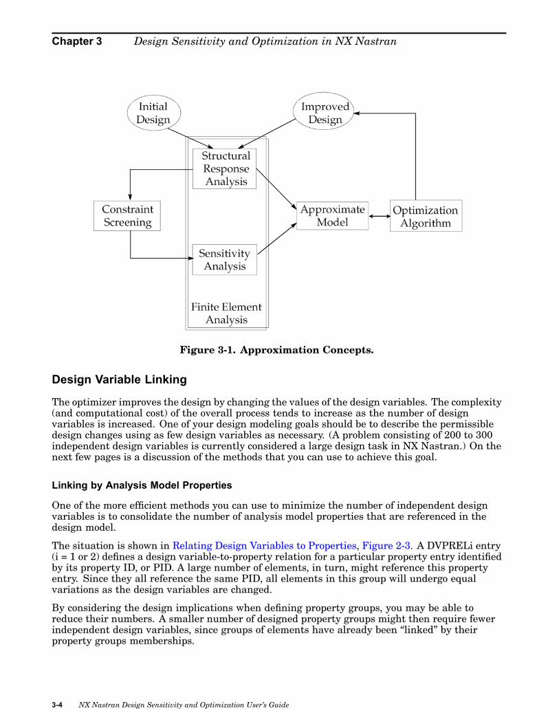
Chapter 3 Design Sensitivity and Optimization in NX Nastran
Figure 3-1. Approximation Concepts.
Design Variable Linking
The optimizer improves the design by changing the values of the design variables. The complexity(and computational cost) of the overall process tends to increase as the number of designvariables is increased. One of your design modeling goals should be to describe the permissibledesign changes using as few design variables as necessary. (A problem consisting of 200 to 300independent design variables is currently considered a large design task in NX Nastran.) On thenext few pages is a discussion of the methods that you can use to achieve this goal.
Linking by Analysis Model Properties
One of the more efficient methods you can use to minimize the number of independent designvariables is to consolidate the number of analysis model properties that are referenced in thedesign model.
The situation is shown in Relating Design Variables to Properties, Figure 2-3. A DVPRELi entry(i = 1 or 2) defines a design variable-to-property relation for a particular property entry identifiedby its property ID, or PID. A large number of elements, in turn, might reference this propertyentry. Since they all reference the same PID, all elements in this group will undergo equalvariations as the design variables are changed.
By considering the design implications when defining property groups, you may be able toreduce their numbers. A smaller number of designed property groups might then require fewerindependent design variables, since groups of elements have already been “linked” by theirproperty groups memberships.
3-4 NX Nastran Design Sensitivity and Optimization User’s Guide

Design Sensitivity and Optimization in NX Nastran
Linking with Linear Relations
If the number of analysis model property entries cannot be reduced, it may be worthwhile toconsider explicit methods of reducing the number of independent design variables. One way youcan do this is by using linear design variable-to-property relations.
The DVPREL1 Bulk Data entry is used to expresses an analysis model property as a linearfunction of design variables or
Equation 3-1.
In this equation, the i-th property pi is a function of the set of design variables x1 through xn.One feature of Eq. 3-1 is that it can be used to express a large number of properties in terms of amuch smaller set of design variables. This is shown in the following example.
Example
Assume an optimal plate thickness distribution is to be determined using a combination ofconstant, linear, and quadratic basis functions as shown in the figure. The design variablesact as multipliers of these basis functions that are, in turn, used to specify the element platethicknesses.
Figure 3-2. Plate Thickness Distribution.
NX Nastran Design Sensitivity and Optimization User’s Guide 3-5

Chapter 3 Design Sensitivity and Optimization in NX Nastran
Figure 3-3. Basis Functions.
Suppose the plate thicknesses are to vary in the x-axis direction, but are to remain constant inthe y-direction. Evaluating the basis functions for each of these ten thickness stations andwriting these design variable-to-thickness relations in matrix form, we get
Equation 3-2.
3-6 NX Nastran Design Sensitivity and Optimization User’s Guide

Design Sensitivity and Optimization in NX Nastran
Reduced Basis FormulationsThe thicknesses of the ten element groups are controlled using only three design variables. Eachof the matrix columns correspond to constant, linear, and quadratic basis functions, respectively.Each column is a vector, and the dimension of each of these vectors is greater than the number ofsuch vectors. Relations of this sort are termed reduced basis formulations.
In general, a reduced basis formulation can be expressed as
Equation 3-3.
The most powerful form of Eq. 3-3 occurs when the number of rows of [T] is much greater thanthe number of columns or M » N. This concept is used extensively in connection with shapeoptimization; a large set of grid coordinate variations can be governed by a much smaller set ofdesign variables (see Relating Design Variables to Shape Changes).
Listing 3-1 shows the Bulk Data entries that can be used to implement the design formulationof Eq. 3-2. Since the reduced basis formulation is just a set of linear equations, DVPREL1Bulk Data entries can be used exclusively. Also, since each of the plate strips are of constantthickness, each element group shares a property Bulk Data entry for a total of ten such entriesover 40 plate elements.
$PSHELL,PID, MID1, T, MID2, 12I/T3 MID3PSHELL, 101, 100, 1.0, 100, , 100PSHELL, 102, 100, 1.0, 100, , 100PSHELL, 103, 100, 1.0, 100, , 100PSHELL, 104, 100, 1.0, 100, , 100PSHELL, 105, 100, 1.0, 100, , 100PSHELL, 106, 100, 1.0, 100, , 100PSHELL, 107, 100, 1.0, 100, , 100PSHELL, 108, 100, 1.0, 100, , 100PSHELL, 109, 100, 1.0, 100, , 100PSHELL, 110, 100, 1.0, 100, , 100$$DESVAR,ID, LABEL, XINIT, XLB, XUB, DELXVDESVAR, 1, X1, 0.33, -1.0, +1.0DESVAR, 2, X2, 0.33, -1.0, +1.0DESVAR, 3, X3, 0.33, -1.0, +1.0$$DVPREL1,ID, TYPE, PID, FID, PMIN, PMAX, C0, , +$+, DVID1, COEF1, DVID2, COEF2, ...DVPREL1,201, PSHELL, 101, 4, 0.01, , , , ++, 1, 1.0, 2, 1.0, 3, 1.0DVPREL1,202, PSHELL, 102, 4, 0.01, , , , ++, 1, 1.0, 2, 0.9, 3, 0.81DVPREL1,203, PSHELL, 103, 4, 0.01, , , , ++, 1, 1.0, 2, 0.8, 3, 0.64DVPREL1,204, PSHELL, 104, 4, 0.01, , , , ++, 1, 1.0, 2, 0.7, 3, 0.49DVPREL1,205, PSHELL, 105, 4, 0.01, , , , ++, 1, 1.0, 2, 0.6, 3, 0.36DVPREL1,206, PSHELL, 106, 4, 0.01, , , , ++, 1, 1.0, 2, 0.5, 3, 0.25DVPREL1,207, PSHELL, 107, 4, 0.01, , , , ++, 1, 1.0, 2, 0.4, 3, 0.16DVPREL1,208, PSHELL, 108, 4, 0.01, , , , ++, 1, 1.0, 2, 0.3, 3, 0.09DVPREL1,209, PSHELL, 109, 4, 0.01, , , , ++, 1, 1.0, 2, 0.2, 3, 0.04
NX Nastran Design Sensitivity and Optimization User’s Guide 3-7

Chapter 3 Design Sensitivity and Optimization in NX Nastran
DVPREL1,210, PSHELL, 110, 4, 0.01, , , , ++, 1, 1.0, 2, 0.1, 3, 0.01
Listing 3-1.
The three design variables, or basis function multipliers, are defined on the three DESVARentries. Each has an initial value of 0.33; therefore, the initial design is defined as that whichhas a one-third contribution from each of the basis functions. The lower and upper bounds onthe design variables are –1.0 and +1.0, respectively, which allow negative as well as positivecontributions from each of the basis functions. The thicknesses are never allowed to assumenegative values due to the 0.01 value of PMIN, or minimum allowable property value, in field6 of each of the DVPREL1 entries.
Since the design model overrides the analysis model in design optimization, the initial analysismodel properties will be set equal to the values computed from the design model specification.For this reason, no effort has been made to calculate the initial thickness distribution on theset of PSHELL entries. These thicknesses have arbitrarily been specified as 1.0 since they willjust be overridden anyway.
A table is output whenever a design model override of the analysis model occurs. A sampleof this table is shown in Design Optimization Output.
Each DVPREL1 entry defines a row in the reducedbasis matrix. The continuation lines of eachentry lists the design variables and coefficients in each of the linear relations. Note that each ofthese continuation lines is simply a row in the reduced basis matrix.
Limitations in Reduced Basis Vector Formulations
In the previous example, the design variable-to-property relations were defined in terms of areduced basis formulation. Essentially, the optimizer’s task is to find the best combination ofthese basis vectors. This combination might not yield the true optimum, and in fact only does soif some combination of the basis vectors is able to uniquely define the optimum. Including otherbasis vectors or allowing each property to vary independently probably will yield a differentoptimum, perhaps even one having a lower structural weight.
Which final design is more useful? If an arbitrary variation of plate thicknesses is permissible(assuming it can be manufactured, of course), and it did not require an unreasonable numberof design variables to obtain this level of generality, then an independent type of relation maybe preferable. That is, each plate element thickness can be a function of just a single designvariable. However, in the preceding example, the basis function approach was able to guaranteethat the resulting plate section had a smoothly varying thickness (in a stepwise fashion, thatis). This may be a more desirable design solution, even though the objective function might bereduced further if this condition were relaxed. In short, the design model formulation representsa statement of design expectations and an implicit acknowledgement of its limitations.
Linking with User-Defined Equations
If the number of analysis model properties cannot be changed or reduced and a reduced basisformulation with DVPREL1 type relations is not sufficient or preferred, use of the DLINK(Design variable LINKing) Bulk Data entry should be considered. Its purpose is to provideexplicit linear relations among the design variables themselves.
The DLINK entries define relations of the type
3-8 NX Nastran Design Sensitivity and Optimization User’s Guide

Design Sensitivity and Optimization in NX Nastran
Equation 3-4.
Eq. 3-4 indicates that design variable linking effectively partitions the vector of design variablesinto an independent set and a dependent set . A DLINK entry defines a single dependentvariable as a linear combination of an independent set of design variables. The dependent designvariable still needs to be defined using a DESVAR entry. The DLINK entry just describes theexplicit linking relations.
A dependent design variable can be used in the design model in exactly the same way as anindependent design variable. It can be used in connection with either property or shapeoptimization, on DVPREL1 and DVPREL2 relations, and so on. There are no restrictions. Theoptimizer, however, need only consider those variables that are in the independent set. Thecorresponding dependent design variable changes are determined from the independent setusing the linking defined by Eq. 3-4.
Example
Quite often, the DLINK entry may be the only way to implement a given design variable linkingscheme. For example, imagine that a rectangular cross-sectional bar consisting of ten elements isto be designed. This bar should be smoothly tapering (in a stepwise fashion, at least), and forpurposes of this example, the shape functions of Figure 3-3, are used.
Suppose the base dimension of this rectangular section is to be a constant 5 mm with the sectionheight as the design variable. This choice yields a total of ten variables similar to the thicknessesof the previous example. However, the only way to describe the cross-sectional properties interms of the cross-sectional dimensions is through the use of equations. The figure below showsa representative cross section and element orientation, and the equations for area, I1 and I2.These equations have been evaluated for an initial h of 10 mm.
Since the design variable-to-property relations for I1 and I2 are not linear in the design variables,DVPREL1 relations cannot be used to express the reduced basis formulation as before. The onlyway this can be implemented is by explicitly linking together the design variables themselvestogether using DLINK entries. Three additional design variables are defined and used as basisfunction multipliers. These design variables form the independent set. The dependent designvariables, linked to the independent set, define the element dimensions. The correspondingelement properties are defined using these dependent variables, which are input to DEQATNentries via DVPREL2 entries.
NX Nastran Design Sensitivity and Optimization User’s Guide 3-9

Chapter 3 Design Sensitivity and Optimization in NX Nastran
The design model definition is given in Listing 3-2. The analysis model contains ten independentPBAR entries since all ten bar sections in the model are to vary.
$PBAR, PID, MID, A, I1, I2PBAR, 101, 100, 5.E-5, 1.042-10,4.167-10PBAR, 102, 100, 5.E-5, 1.042-10,4.167-10PBAR, 103, 100, 5.E-5, 1.042-10,4.167-10PBAR, 104, 100, 5.E-5, 1.042-10,4.167-10PBAR, 105, 100, 5.E-5, 1.042-10,4.167-10PBAR, 106, 100, 5.E-5, 1.042-10,4.167-10PBAR, 107, 100, 5.E-5, 1.042-10,4.167-10PBAR, 108, 100, 5.E-5, 1.042-10,4.167-10PBAR, 109, 100, 5.E-5, 1.042-10,4.167-10PBAR, 110, 100, 5.E-5, 1.042-10,4.167-10$$...INDEPENDENT DESIGN VARIABLE SET:$DESVAR,ID, LABEL, XINIT, XLB, XUB, DELXVDESVAR, 1, X1, 1.0, -1.0, +1.0DESVAR, 2, X2, 0.0, -1.0, +1.0DESVAR, 3, X3, 0.0, -1.0, +1.0$$...DEPENDENT DESIGN VARIABLE SET:$DESVAR,ID, LABEL, XINIT, XLB, XUB, DELXVDESVAR, 11, H1, .01, 1.E-4, 1.0DESVAR, 12, H2, .01, 1.E-4, 1.0DESVAR, 13, H3, .01, 1.E-4, 1.0DESVAR, 14, H4, .01, 1.E-4, 1.0DESVAR, 15, H5, .01, 1.E-4, 1.0DESVAR, 16, H6, .01, 1.E-4, 1.0DESVAR, 17, H7, .01, 1.E-4, 1.0DESVAR, 18, H8, .01, 1.E-4, 1.0DESVAR, 19, H9, .01, 1.E-4, 1.0DESVAR, 20, H10, .01, 1.E-4, 1.0$$...DESIGN VARIABLE LINKING, Hj = Hj(X1,X2,X3) ; j=11,20:$DLINK, ID, DDVID, CO, CMULT, IDV1, C1, IDV2, C2, +$+, IDV3, C3, ...DLINK, 21, 11, , .01, 1, 1.0, 2, 1.0, ++, 3, 1.0DLINK, 22, 12, , .01, 1, 1.0, 2, 0.9, ++, 3, 0.81DLINK, 23, 13, , .01, 1, 1.0, 2, 0.8, ++, 3, 0.64DLINK, 24, 14, , .01, 1, 1.0, 2, 0.7, ++, 3, 0.49DLINK, 25, 15, , .01, 1, 1.0, 2, 0.6, ++, 3, 0.36DLINK, 26, 16, , .01, 1, 1.0, 2, 0.5, ++, 3, 0.25DLINK, 27, 17, , .01, 1, 1.0, 2, 0.4, ++, 3, 0.16DLINK, 28, 18, , .01, 1, 1.0, 2, 0.3, +
+, 3, 0.09DLINK, 29, 19, , .01, 1, 1.0, 2, 0.2, ++, 3, 0.04DLINK, 30, 20, , .01, 1, 1.0, 2, 0.1, ++, 3, 0.01$$...DESIGN EQUATION:DEQATN 40 I2(H) = 0.005*H**3/12.$$...TYPE-2 DESIGN VARIABLE TO PROPERTY RELATIONS:$DVPREL2,ID, TYPE, PID, FID, PMIN, PMAX, EQID, , +$+, DESVAR, DVID1, DVID2, ..., , , , , +$+, DTABLE, CID1, CID2, ...
3-10 NX Nastran Design Sensitivity and Optimization User’s Guide

Design Sensitivity and Optimization in NX Nastran
DVPREL2,41, PBAR, 101, 6, 1.0E-12,, 40, , ++, DESVAR, 11DVPREL2,42, PBAR, 102, 6, 1.0E-12,, 40, , ++, DESVAR, 12DVPREL2,43, PBAR, 103, 6, 1.0E-12,, 40, , ++, DESVAR, 13DVPREL2,44, PBAR, 104, 6, 1.0E-12,, 40, , ++, DESVAR, 14DVPREL2,45, PBAR, 105, 6, 1.0E-12,, 40, , ++, DESVAR, 15DVPREL2,46, PBAR, 106, 6, 1.0E-12,, 40, , ++, DESVAR, 16DVPREL2,47, PBAR, 107, 6, 1.0E-12,, 40, , ++, DESVAR, 17DVPREL2,48, PBAR, 108, 6, 1.0E-12,, 40, , ++, DESVAR, 18DVPREL2,49, PBAR, 109, 6, 1.0E-12,, 40, , ++, DESVAR, 19DVPREL2,50, PBAR, 110, 6, 1.0E-12,, 40, , ++, DESVAR, 20
Listing 3-2.
The basis function multipliers are x1, x2, and x3. Their initial values of 1.0, 0.0, and 0.0correspond to a constant height beam section. Negative lower bounds allow a negativecontribution from any of the basis functions.
The dependent variables are defined using DESVAR entries 11 through 20. Since the dependentvariables define the bar element heights (i.e., nonnegative physical dimensions), their lowerbounds are specified as small positive numbers to avoid negative bar cross-sectional heights.
The optimizer never proposes a design that is outside the bounds placed on the designvariables. (This often results in a more effective method of applying bounds than is PMINor PMAX on the DVPRELi Bulk Data entries.)
The dependent variables are related to the independent set on DLINK entries 21 through 30.Each DLINK entry defines a row of the reduced basis matrix similar to the DVPREL1 entries ofthe previous example. This dependent set of design variables is input to equations in DVPREL2type relations.
DVPREL2 entries 41 through 50 specify the area moments of inertia in plane 2 for each of thebar element properties as indicated by the 6 in field 5. Note that they all reference the sameDEQATN entry 40 containing the functional relation between h and I2. Each of the DVPREL2continuations describe the equation input arguments, consisting of just a single design variable.The 1.0E–12 value for PMIN in field 6 ensures that the property does not take on values lessthan this bound.
For brevity, the equations for areas and I1 for each property group have not been listed sincethe method used to define these relations is identical to that shown here. Without relating thedesign variables to changes in bar areas, weight minimization, for example, will not be possible.Also, if stresses due to bending are in the design model, the dependence of the stress recoverylocations on the design variables should also be defined.
Constraint ScreeningConstraint screening is an automatic process for both design sensitivity and optimization andconsists of two parts: regionalization and deletion. You can override some of the defaultsassociated with this process by
• Providing explicit region IDs on the DRESP1 and DRESP2 entries.
NX Nastran Design Sensitivity and Optimization User’s Guide 3-11

Chapter 3 Design Sensitivity and Optimization in NX Nastran
• Using DSCREEN entries to override key screening parameters.
There is often little need to override the constraint screening defaults, since these perform wellin the vast majority of cases. However, computational efficiency can sometimes be gained bymodifying these defaults in special cases. This section outlines constraint screening so that youcan make effective use of it should the occasion arise.
Basic Concepts
The basic assumption behind constraint screening is that most structural optimization problemscontain more constraints than are necessary to adequately guide the design. For example,suppose bending stresses for every beam element are required to be less than some allowableupper limit. Not every element in the model may be critically loaded, while those that are mayundergo more or less similar changes as the design is modified. This is a case of extraneous andredundant design data. If the constraints can be “filtered” in a consistent manner, a considerableincrease in efficiency may be realized.
A response that is to be constrained must first be defined on either a DRESP1 or DRESP2entry. Response lower and upper bounds are set with a DCONSTR entry. For the j-th responsethis definition yields
Equation 3-5.
NX Nastran uses these bounds to create a pair of normalized constraints as
Equation 3-6.
where the absolute values of the bounds are used as normalizing factors.
This normalization provides a convenient method of screening the constraints. For example, anynormalized constraint with a value of +0.5 has violated its bound by 50%, while a constraint witha value of –0.5 is within 50% of its bound. We might argue that it may not be necessary to retainevery constraint, just those that are greater than some normalized value.
Constraint Deletion
Figure 3-4 represents a group of constraints in bar chart form. In constraint deletion, anyconstraint exceeding the truncation threshold value (shown as TRS in the figure) is retainedfor the current design cycle. Those constraints whose values are less than this threshold aretemporarily deleted for the current cycle. These deleted constraints may again become activeduring subsequent design cycles and thus retained.
3-12 NX Nastran Design Sensitivity and Optimization User’s Guide
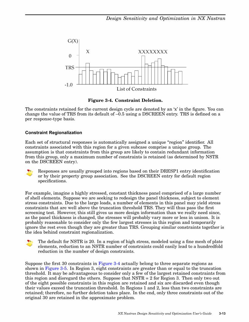
Design Sensitivity and Optimization in NX Nastran
Figure 3-4. Constraint Deletion.
The constraints retained for the current design cycle are denoted by an ‘x’ in the figure. You canchange the value of TRS from its default of –0.5 using a DSCREEN entry. TRS is defined on aper response-type basis.
Constraint Regionalization
Each set of structural responses is automatically assigned a unique “region” identifier. Allconstraints associated with this region for a given subcase comprise a unique group. Theassumption is that constraints from this group are likely to contain redundant informationfrom this group, only a maximum number of constraints is retained (as determined by NSTRon the DSCREEN entry).
Responses are usually grouped into regions based on their DRESP1 entry identificationor by their property group association. See the DSCREEN entry for default regionspecifications.
For example, imagine a highly stressed, constant thickness panel comprised of a large numberof shell elements. Suppose we are seeking to redesign the panel thickness, subject to elementstress constraints. Due to the large loads, a number of elements in this panel may yield stressconstraints that are well above the truncation threshold TRS. They will thus pass the firstscreening test. However, this still gives us more design information than we really need since,as the panel thickness is changed, the stresses will probably vary more or less in unison. It isprobably reasonable to consider only the few largest stresses in this region and temporarilyignore the rest even though they are greater than TRS. Grouping similar constraints together isthe idea behind constraint regionalization.
The default for NSTR is 20. In a region of high stress, modeled using a fine mesh of plateelements, reduction to an NSTR number of constraints could easily lead to a hundredfoldreduction in the number of design constraints.
Suppose the first 30 constraints in Figure 3-4 actually belong to three separate regions asshown in Figure 3-5. In Region 3, eight constraints are greater than or equal to the truncationthreshold. It may be advantageous to consider only a few of the largest retained constraints fromthis region and disregard the others. Suppose that NSTR = 2 for Region 3. Then only two outof the eight possible constraints in this region are retained and six are discarded even thoughtheir values exceed the truncation threshold. In Regions 1 and 2, less than two constraints areretained; therefore, no further deletion takes place. In the end, only three constraints out of theoriginal 30 are retained in the approximate problem.
NX Nastran Design Sensitivity and Optimization User’s Guide 3-13

Chapter 3 Design Sensitivity and Optimization in NX Nastran
Figure 3-5. Constraint Regionalization.
Constraint Screening and Sensitivity Analysis
Constraint screening precedes sensitivity analysis as can be seen from the flowchart in Figure 3-1and in the detailed Solution 200 flowchart in Design Modeling for Sensitivity and Optimization.The default values of TRS and NSTR are usually fine for most design optimization problems;however, for design sensitivity analysis, these default values may not be satisfactory. It maybe that some of the responses for which you had requested that sensitivities are screenedout. To ensure that all responses are retained, you may need to set TRS to a large negativenumber, perhaps –10. or –100. Also, depending on the number of responses per region, it may benecessary to increase NSTR. This combination ensures that all constraints pass both levels ofscreening and all responses are retained for sensitivity analysis. This procedure is the only wayto turn off the screening.
Formal Approximations
NX Nastran uses formal approximation to avoid the high cost associated with repeated finiteelement analyses during design optimization. Two basic types of approximation are used
• Direct variable approximations.
• Reciprocal variable approximations.
These approximations are used in various ways according to three different methods availablein NX Nastran:
• Direct Approximations (APRCOD = 1).
• Mixed Approximations (APRCOD = 2 default).
• Convex Linearization (APRCOD = 3).
A DOPTPRM entry is used to select APROD.
3-14 NX Nastran Design Sensitivity and Optimization User’s Guide

Design Sensitivity and Optimization in NX Nastran
Choosing to override the default approximation is usually problem-dependent, and often withoutstrict rules or guidelines. This subsection presents theoretical details that may help you decidewhen such an override might be appropriate.
The formal approximations used in NX Nastran are all based on simple first-order Taylor seriesexpansions. The general form of this expansion is
Equation 3-7.
Approximation ErrorsThe required derivative information is available from the design sensitivity analysis as outlined
in Design Sensitivity Analysis. Note that the approximate response, , in Eq. 3-7.Eq. 3-7 is linear in the design variable change Δx. Thus, we expect some error when we try toapproximate responses that are actually nonlinear in Δx. Figure 1-16 in Structural Optimizationshows how the error is a function of Δx.
Move Limits and ApproximationsDuring approximate optimization, the code places limits on the maximum allowable moves inthe design space in order to minimize the errors associated with these approximations. In NXNastran, move limits are placed both on property as well as design variable changes. Move limitsare discussed in Optimization with Respect to Approximate Models.
Direct Approximations
A direct variable approximation linearizes the function directly in terms of the design variables.For the j-th constraint function, the direct approximation is written as
Equation 3-8.
where the subscript D indicates a direct approximation.
The quantity represents a total vector move in the design space from the initial design .The partial derivatives ∂gj/∂xi are available from the design sensitivity analysis. An equationsimilar to Eq.3-8 can be written for the objective function, where F replaces g in the expression.
Reciprocal Approximations
The first-order Taylor series expansions of Eq. 3-8 can alternately be expressed in terms ofreciprocal variables. This choice turns out to be quite useful for those responses that areinversely proportional to the design variables. This simple idea can be easily shown in the case
NX Nastran Design Sensitivity and Optimization User’s Guide 3-15
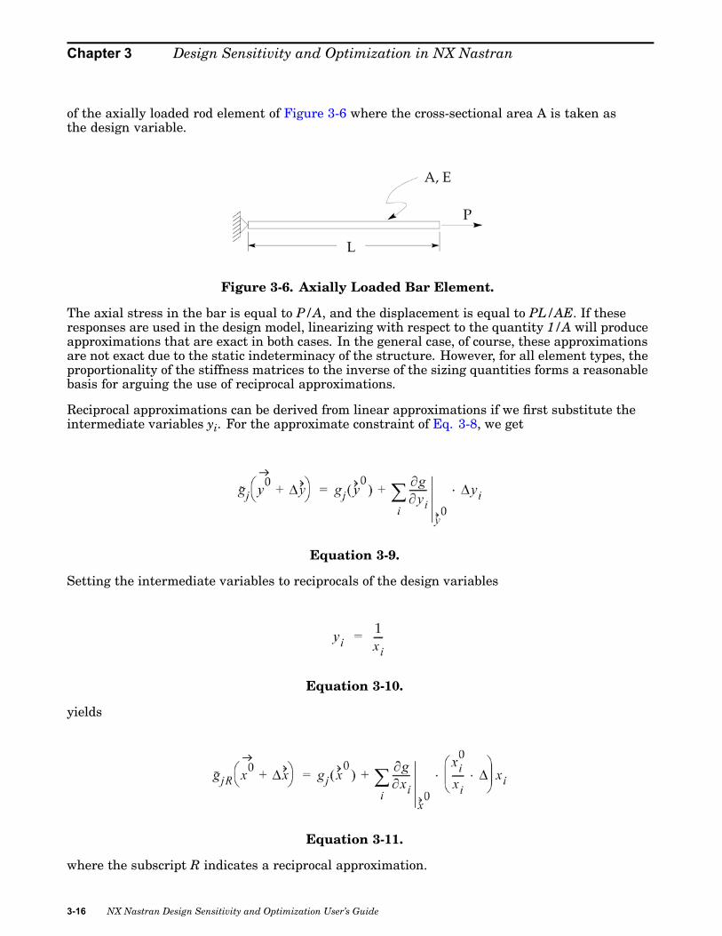
Chapter 3 Design Sensitivity and Optimization in NX Nastran
of the axially loaded rod element of Figure 3-6 where the cross-sectional area A is taken asthe design variable.
Figure 3-6. Axially Loaded Bar Element.
The axial stress in the bar is equal to P/A, and the displacement is equal to PL/AE. If theseresponses are used in the design model, linearizing with respect to the quantity 1/A will produceapproximations that are exact in both cases. In the general case, of course, these approximationsare not exact due to the static indeterminacy of the structure. However, for all element types, theproportionality of the stiffness matrices to the inverse of the sizing quantities forms a reasonablebasis for arguing the use of reciprocal approximations.
Reciprocal approximations can be derived from linear approximations if we first substitute theintermediate variables yi. For the approximate constraint of Eq. 3-8, we get
Equation 3-9.
Setting the intermediate variables to reciprocals of the design variables
Equation 3-10.
yields
Equation 3-11.
where the subscript R indicates a reciprocal approximation.
3-16 NX Nastran Design Sensitivity and Optimization User’s Guide

Design Sensitivity and Optimization in NX Nastran
Approximation Methods
Three different approximation methods are available in NX Nastran. You can select any one ofthem using the APRCOD field on the DOPTPRM entry. These methods are as follows:
• APRCOD = 1: This specifies that direct approximations Eq. 3-8 are to be used for theobjective function as well as all constraints. The resulting approximate optimization is thenperformed with respect to an entirely linear approximate design space. You should use thisoption if you know that the structural responses are well-approximated by linear functions inthe design variables. Otherwise, without carefully chosen move limits, a greater number ofapproximate optimization cycles may be required before convergence is achieved.
• APRCOD = 2: (Default) This choice specifies that mixed approximations (or more precisely,a mixture of approximations) are to be used. Direct approximations are used for volume,weight, element force, and buckling load responses, while reciprocal approximations are usedfor all other response types. This method works well in a wide variety of problem types.Because of its reliability, it has been selected as the default method.
• APRCOD = 3: This selects the convex linearization method. Essentially, this method chooseseither a direct or reciprocal constraint approximation depending on which one providesthe larger estimation of the constraint function. In other words, this method chooses themore conservative of the two approximations.
For example, the direct approximation for the j-th constraint is
Equation 3-12.
while the reciprocal approximation is
Equation 3-13.
Since both approximations are readily available (both use the same gradient information),the choice of which to use can be made just by looking at the sign of the difference betweenthe two:
NX Nastran Design Sensitivity and Optimization User’s Guide 3-17

Chapter 3 Design Sensitivity and Optimization in NX Nastran
Equation 3-14.
Since the squared term in the expression is always positive, the choice depends on the signof the product:
• if Use the direct approximation for xi since it yields a largerestimate of constraint value.
• if Use the reciprocal approximation for xisince it yields a largerestimate of constraint value.
Equation 3-15.
This criterion is applied on an individual design variable basis. Thus, a combination of directand reciprocal approximations can be made for a single constraint.
For convex linearization, the objective function is always linearized, regardless of itsresponse type.
Modeling GuidelinesThere are several situations where the default mixed method (APRCOD=2) is not applicableand therefore not recommended. The first is when basis vectors for either property orshape optimization are used. In this case, the physical justification for the use of reciprocalapproximations does not apply (see Reciprocal Approximations earlier in this chapter), andeither direct approximations (or perhaps even convex linearization) should be used instead.
The second situation occurs if design variables can pass through zero during the course ofoptimization. This can occur if the lower bound on the DESVAR entry is a negative quantityand the upper bound is positive. In this case, APRCOD is automatically set to 1 to avoidill-conditioning about the zero value of the design variable.
Finally, experience has also shown that the mixed method is not always the best performerfor dynamic response optimization tasks. For these highly nonlinear responses, directapproximations, coupled with more stringent move limits are often more reliable.
Advanced Topics in ApproximationsThe direct and reciprocally-approximated constraints of Eq. 3-8 and Eq. 3-11 require theevaluation of function derivatives with respect to design variables. Computing these functionderivatives is complicated somewhat by design variable-to-property relations, which may beeither type-1 or type-2 (DVPREL1 or DVPREL2), and responses, which may be either first- orsecond-level (DRESP1 or DRESP2).
3-18 NX Nastran Design Sensitivity and Optimization User’s Guide

Design Sensitivity and Optimization in NX Nastran
To accommodate type-1 and type-2 design variable-to-property relations, the concept of a designvariable is generalized internally in the code. For type-1 relations, the basis for the constraintand objective function approximations is the set of independent design variables. For type-2relations, this basis is the set of properties defined on the DVPREL2 entries. For the j-thconstraint, these choices result in
Equation 3-16.
Equation 3-17.
where:
Equation 3-18.
Similar expressions can also be written for the objective function. The benefit of thisgeneralization is that properties are computed precisely in Eq. 3-18 for a given change in designvariables. The approximation in Eq. 3-17 thus retains all of the non-linearities of the DVPREL2relations, yielding a more accurate approximation.
Depending on whether the response quantities are first- or second-level, the derivatives areevaluated as follows. If we let the quantity f represent either an objective or a constraintfunction, then for first-level responses we have
Equation 3-19.
Equation 3-20.
NX Nastran Design Sensitivity and Optimization User’s Guide 3-19

Chapter 3 Design Sensitivity and Optimization in NX Nastran
where the superscript on r(1) denotes a first-level (DRESP1) response.
For objectives or constraints that are functions of second-level responses, we have
Equation 3-21.
Equation 3-22.
where r(2) is a second-level response.
In general, these second-level responses can be functions of design variables, table constants,first-level responses, and grid coordinates. That is,
Equation 3-23.
Chain rule differentiation of Eq. 3-23 with respect to the i-th design variable gives
Equation 3-24.
where xi is used here to indicate either a design variable or a “design property” (DVPREL2property), see Eq. 3-21 or Eq. 3-22. (δ is used to denote partial differentiation with respect to thedesign variables appearing explicitly in rj.)
In NX Nastran, the terms in Eq. 3-19 through Eq. 3-24 are computed as follows:
1. These quantities are available directly from the semi-analytic sensitivityanalysis.
2. Depending on whether is an objective or constraint, these terms are availableas
3-20 NX Nastran Design Sensitivity and Optimization User’s Guide

Design Sensitivity and Optimization in NX Nastran
Equation 3-25.
Equation 3-26.
3.
This term is approximated using central differences and the equation solving utility inNX Nastran as
Equation 3-27.
FDCH = 1.0E–3, FDCHM = 1.0E–6.
where Δxi = FDCH · xi0
and if FDCH · xi0 < FDCHM,
then Δxi = FDCHM.
4.
This term is also approximated using central differences and the equation utility as
Equation 3-28.
NX Nastran Design Sensitivity and Optimization User’s Guide 3-21

Chapter 3 Design Sensitivity and Optimization in NX Nastran
where Δrk(1) is determined using FDCH and FDCHM as in item 3.
5.
This term is approximated using central differences as
Equation 3-29.
where {ΔG}l is the variation in the coordinates of the l grid point and {G0} represents thebaseline coordinates of those grids used in the expression for rj
(2).
{ΔG}l is determined as
Equation 3-30.
where FDCHM is used for any component that is less than this amount.
6.
This information is available directly from the basis vectors for shape optimization. Notethat each term of a basis vector defines the (constant) rate of change of a grid coordinategiven a change in a design variable.
3.2 Design Sensitivity AnalysisDesign sensitivity analysis computes the rates of change of structural response quantities withrespect to changes in design variables. Since these partial derivatives provide the essentialgradient information to the optimizer, they are always computed in connection with designoptimization. Sensitivity analysis is always performed automatically in NX Nastran wheneverdesign optimization is requested. There may be times when you want the software to computejust the sensitivity coefficients and not perform optimization. You can then use this sensitivityinformation to perform parametric design studies or to link with your own optimizer.
This section presents the theoretical basis for design sensitivity analysis in NX Nastran. It showshow to request sensitivity analysis, describes how the sensitivity coefficients are computed,and presents modeling guidelines.
3-22 NX Nastran Design Sensitivity and Optimization User’s Guide

Design Sensitivity and Optimization in NX Nastran
General Considerations
A design sensitivity coefficient is defined as the rate of change of a particular response quantity rwith respect to a change in a design variable x or ∂r/∂x. These coefficients are evaluated at a
particular design characterized by the vector of design variables , giving
Equation 3-31.
where subscripts are used to indicate the i-th design variable and the j-th response. Eq. 3-31 isjust the slope of the response with respect to xi as is shown in Eq. 3-7.
Figure 3-7. Design Sensitivity Coefficient—Graphical Interpretation.
For Which Responses Are Sensitivities Computed?
Sensitivities are computed for all of the responses (both first- and second-level) that are used todefine the objective function and retained constraints.
Recall from Approximation Concepts in Design Optimization that sensitivity analysis is alwaysperformed after the constraint screening phases are completed (Figure 3-1). Thus, fewerresponse sensitivities may be computed than there are responses defined in the design model.Of course, this is the goal since the computational effort associated with sensitivity analysis isreduced. (If you wish to force the computation of all sensitivities for all responses defined in thedesign model, you can effectively disable the screening process by using a large negative TRS
NX Nastran Design Sensitivity and Optimization User’s Guide 3-23

Chapter 3 Design Sensitivity and Optimization in NX Nastran
on the DSCREEN Bulk Data entries along with a large NSTR if necessary. See the DSCREENentry description in Input Data for further details.)
Requesting Sensitivity Analysis Output
Design sensitivities are output in the form of Eq. 3-1. In Solution 200, you request designsensitivity analysis and output with the following Bulk Data parameter definition:
PARAM, OPTEXIT, ±4
You can also request design sensitivity coefficient output with an OPTEXIT value of 7. SeeSolution 200 Program Flow), Solution 200 Program Flow, for details.
An OPTEXIT of ±4 prints the sensitivity coefficients to the standard output file. A value of –4outputs the coefficients in binary form using OUTPUT4 formats.
Identifying the Sensitivity Coefficients
If requested by a PARAM,OPTEXIT,±4 or 7, sensitivity coefficients are output in the matrixDSCM2. Each column in this matrix corresponds to a particular response quantity, while eachrow corresponds to a design variable. The component of the i-th row and j-th column is
Equation 3-32.
A correlation matrix is also output to help identify the column order of the individual designresponses. The row order in DSCM2 corresponds to the design variables defined on theset of DESVAR entries sorted by increasing design variable ID. See Output Features andInterpretation, Design Sensitivity Output, for examples illustrating the interpretation of thisoutput.
Internal Representation of the Sensitivity Coefficients in NX Nastran
The sensitivity coefficients represented in Eq. 3-32 are actually computed and output in this formonly if you have requested them via a PARAM,OPTEXIT,±4 or 7. For reasons of efficiency as wellas accuracy, NX Nastran uses a slightly different internal representation of these coefficients,depending on how the design variables are related to the analysis model properties.
For DVPREL1 type relations, the set of independent design variables is taken as the basis forthe design sensitivity coefficients (see the DLINK entry for a definition of independent anddependent design variables). This is an efficient choice since a large number of properties may bea function of a much smaller set of design variables.
For DVPREL2 relations, the basis for sensitivity analysis is taken to be the set of analysis modelproperties referenced on all of these second-level relations. Inside the code, the sensitivities arethen
3-24 NX Nastran Design Sensitivity and Optimization User’s Guide

Design Sensitivity and Optimization in NX Nastran
Equation 3-33.
Choosing properties as the basis greatly improves the accuracy of the approximate responsesused in design optimization. Since an explicit relation between the properties and the associateddesign variables is given by the DVPREL2–DEQATN entry pair, this information can be usedto evaluate the properties for a given change in the set of design variables. Computing thesensitivities with respect to the design variables would have linearized this relation, resultingin a less accurate approximation.
To summarize, the sensitivity coefficients used internally in NX Nastran are
Equation 3-34.
where NIDV is the number of independent design variables and NIPR is the set of propertiesdefined on all DVPREL2 entries.
To illustrate the advantage in using a mixed design variable-property basis, consider thenormalized lower-bound constraint in Eq. 2-29, Defining the Constraints.
Equation 3-35.
This is the form of the lower-bound constraint that is automatically generated in NX Nastranfrom the DCONSTR entry data. For a finite move in the design space Δx, the approximatedconstraint is
Equation 3-36.
NX Nastran Design Sensitivity and Optimization User’s Guide 3-25

Chapter 3 Design Sensitivity and Optimization in NX Nastran
Since the response is only approximate, the constraint is approximate as well. For responsesthat depend on properties that are linear functions of the design variables (DVPREL1), theapproximation is
Equation 3-37.
while, for responses that depend on the properties that are nonlinear functions of the designvariables (DVPREL2),
Equation 3-38.
where the properties at the perturbed design in Eq. 3-8 can be evaluated precisely from theinput equations DEQATN. Eq. 3-37 and Eq. 3-38 show the advantage of generalizing the basis toinclude not only design variables but also design properties.
Sensitivities of Static Responses
Requesting Static Response Sensitivities
To compute the sensitivities of static responses, you need to
• Define a design model (see Design Modeling for Sensitivity and Optimization).
• Define a static analysis subcase in Solution 200 using the Case Control command
ANALYSIS = STATICS
• Either request sensitivity coefficient output with the Bulk Data parameter assignment
PARAM, OPTEXIT, 4orPARAM, OPTEXIT, 7
• Or, invoke Solution 200 for design optimization. (Static response sensitivities are computedautomatically in design optimization if static responses are present in the design model.)
Theory
For a given structure with specified geometry, material properties, and boundary conditions, adisplacement-based linear static analysis computes the displacement responses due to theapplied loads. All other static responses such as stresses and strains are determined from thedisplacement solution. For an arbitrary response r, the functional dependency on displacement iswritten as
3-26 NX Nastran Design Sensitivity and Optimization User’s Guide

Design Sensitivity and Optimization in NX Nastran
Equation 3-39.
In the design context, the displacement solution is an implicit function of the design variables.That is,
Equation 3-40.
Since all other design responses may be functions of these displacements, these are implicit inthe design variables as well. These can include both first- as well as second-level responsetypes where
Equation 3-41.
In NX Nastran, the sensitivities of these responses with respect to changes in the designvariables are approximated using first forward finite differences as
Equation 3-42.
where is the j-th design response.
Eq. 3-42 accounts for the functional dependency of the response on both the design variables andthe displacement solution. However, since the displacements are implicit functions of the designvariables, the quantity Δu must be computed as
Equation 3-43.
Eq. 3-43 requires that the displacement sensitivity be known. The sensitivities can be computedby differentiating the equations of static equilibrium
Equation 3-44.
to obtain
NX Nastran Design Sensitivity and Optimization User’s Guide 3-27

Chapter 3 Design Sensitivity and Optimization in NX Nastran
Equation 3-45.
This equation is solved in NX Nastran to obtain the displacement sensitivities. Once these areknown, the sensitivities of all necessary responses can be found from Eq. 3-42 and Eq. 3-43.
Computationally, the solution of Eq. 3-45 is identical to the solution for Eq. 3-44 except that theydiffer in the right-hand side load vectors. In fact, the cost of the displacement sensitivity solutioncan be reduced if the stiffness matrix, already available in decomposed form as a result of thefinite element solution, is used. This observation is taken advantage of in NX Nastran.
Note that the right-hand side of Eq. 3-45 (often referred to as the pseudo-load vector), includesthe partial derivatives ∂{P}/∂xi and ∂[K]/∂xi. Since these are generally implicit functions of thedesign variables, these derivatives are approximated using finite differences as follows:
• For property optimization, unless CDIF = ‘YES’,
Equation 3-46.
• For shape optimization, or if CDIF = ‘YES’
Equation 3-47.
For property optimization, the size of the move Δx is given by
Equation 3-48.
3-28 NX Nastran Design Sensitivity and Optimization User’s Guide

Design Sensitivity and Optimization in NX Nastran
where DELB is given on the DOPTPRM Bulk Data entry. See Shape Sensitivity (later in thischapter) for the corresponding grid variation for shape optimization.
As a result of these finite difference approximated terms in the pseudo-load vector, the solution ofEq. 3-45 is frequently referred to as a semianalytic one. A similar approach is used in the otheranalysis disciplines as well as being discussed in the following sections.
Even though Eq. 3-42 through Eq. 3-48 are expressed in terms of the design variables xi, independently varying properties, pi , may also be used if DVPREL2 relations appear inthe design model. In practice then, the set of design variables in the preceding equationsis generalized in the code to include not only the independent design variables but also theindependently varying properties.
Eigenvalue Response Sensitivities
Requesting Eigenvalue Response Sensitivities
To compute eigenvalue sensitivities, you need to
• Define a design model (see Design Modeling for Sensitivity and Optimization).
• Define a normal modes subcase using the Case Control commandANALYSIS = MODES
Eigenvalue response sensitivities are computed automatically in connection with designoptimization. If you do not want to perform optimization, you can request sensitivity analysiswith the Bulk Data parameter assignment.
PARAM, OPTEXIT, 4
Theory
Normal modes analysis can be requested in Solution 200 by setting the Case Control command,ANALYSIS = MODES. This setting invokes both a normal modes analysis as well as a sensitivityanalysis if either sensitivity or optimization is requested.
The eigenvalue equation is
Equation 3-49.
where λn and φn are the n-th eigenvalue and eigenvector, respectively. [K] is the structuralstiffness, and [M] is the structural mass.
The governing Eq. 3-49 can be differentiated with respect to the i-th design variable xi to yield,
Equation 3-50.
When Eq. 3-50 is premultiplied by φnT, the first term is zero. Eq. 3-50 can then be solved forthe eigenvalue derivatives
NX Nastran Design Sensitivity and Optimization User’s Guide 3-29

Chapter 3 Design Sensitivity and Optimization in NX Nastran
Equation 3-51.
In practice, the solution to the above equation is based on a semi-analytic approach. Thederivatives of the mass and stiffness matrices are approximated using finite differences of theform in Eq. 3-46 and Eq. 3-47. Eq. 3-51 is solved for each retained eigenvalue referenced in thedesign model and for each design variable. This equation is valid only for the case of distincteigenvalues.
Buckling Load Factor Sensitivities
Requesting Buckling Load Factor Sensitivities
To obtain buckling load factor sensitivities in Solution 200, you need to:
• Define a design model (see Design Modeling for Sensitivity and Optimization).
• Define a buckling subcase in Solution 200 with the Case Control command
ANALYSIS = BUCK
Buckling load factor sensitivities are computed automatically in connection with designoptimization. If you just want to compute and output the sensitivity coefficients, you may do sowith the Bulk Data parameter assignment
PARAM, OPTEXIT, 4
Theory
The derivation of buckling sensitivity similar is similar to that of eigenvalue sensitivities. Theequation for determining of the buckling load factor λ is
Equation 3-52.
Differentiating this expression and solving for the buckling load factor sensitivities yields
Equation 3-53.
As before, this equation is solved semi-analytically by approximating the structural propertymatrix derivatives using finite differences.
3-30 NX Nastran Design Sensitivity and Optimization User’s Guide

Design Sensitivity and Optimization in NX Nastran
Differential Stiffness Approximations
The approximation of the differential stiffness is worth discussing. This stiffness is a functionnot only of geometry but of displacement as well
Equation 3-54.
In the finite difference approximation, [Kd] should be approximated for the perturbedconfiguration as
Equation 3-55.
since the displacements are also implicit functions of the design variables. However, in NXNastran, this displacement variation is ignored, resulting in
Equation 3-56.
In most cases, Eq. 3-56 is a reasonable approximation. Eq. 3-55 is an often unnecessary, costlyalternative. However, if the optimization results suggest that the sensitivities are not of sufficientaccuracy, one (or both) of two options might be used. The first is to use the DOPTPRM entry todecrease DELB (the finite difference move parameter) by one or more orders of magnitude. Thisreduction might also be coupled with central difference approximations. (Setting the Bulk Dataparameter CDIF to YES forces central differences.) The second option might be to reduce themove limits using DELP and DELX on the DOPTPRM entry and DELXV on the DESVAR entries.The goal of these changes is to improve the quality of the approximation seen by the optimizer.
The parameter DSNOKD can be used to suppress the computation of the differentialstiffness derivative. See Parameters for Design Sensitivity and Optimization.
Shape Sensitivity
Shape sensitivities are computed in Solution 200 whenever design variables are used to describeshape changes. They are computed automatically in connection with design optimization or if asensitivity analysis alone (PARAM, OPTEXIT±4) is requested.
In shape optimization, the design responses are functions of the shape-defining design variables.Recall the reduced basis formulation used in connection with shape optimization
NX Nastran Design Sensitivity and Optimization User’s Guide 3-31

Chapter 3 Design Sensitivity and Optimization in NX Nastran
Equation 3-57.
In Eq. 3-57, changes in grid coordinates {ΔG} are expressed in terms of changes in the designvariables {Δx}, and the shape basis vectors [T].
For semianalytic shape sensitivities, grid coordinates are perturbed a finite amount
Equation 3-58.
The subscript i in Eq. 3-58 characterizes the relation as a variation in shape for the i-th designvariable.
Ei is the maximum strain energy norm computed using the {T}i basis vector. STPSCL is a scalingfactor (default=1.0) that can be changed using the DOPTPRM Bulk Data entry.
The maximum strain energy norm used in Eq. 3-58 component is computed by first determiningthe grid “forces” due to a shape basis vector “displacement”:
Equation 3-59.
These forces can be used to compute a strain energy per grid as
Equation 3-60.
Eq. 3-60 is an open product, resulting in a vector of strain energies at each grid. Locating themaximum term in the vector and taking its square root yields
Equation 3-61.
We get one such Ei for each design variable-shape basis vector pair. This has been found to yielda consistent set of finite difference move parameters for shape optimization.
Dynamic Response Sensitivities
Dynamic response sensitivities are computed in Solution 200 in connection with designsensitivity analysis and optimization. The following disciplines are available:
• Direct frequency
• Modal frequency
3-32 NX Nastran Design Sensitivity and Optimization User’s Guide
Design Sensitivity and Optimization in NX Nastran
• Modal transient
See the DRESP1 Bulk Data entry description for a list of the response types supported for theabove analysis disciplines.
General Considerations
The complete stiffness matrix for dynamic response analysis consists of a superposition fromdamping as well as direct matrix input:
Equation 3-62.
where:
[K1] = structural stiffnessg = uniform structural damping coefficient PARAM,G
ge = structural damping coefficient on a MAT entry[K2] = direct matrix input at grids DMIG
Since design variables can only be related to analysis model properties that appear on propertyentries or to grid locations, a functional relation between design variables and g or ge cannot beprescribed. The structural damping contributions are assumed constant for design sensitivity.They are accounted for in the analysis, but do not vary as a function of the design variables.Similarly, the direct matrix input quantities cannot be expressed as functions of the designvariables since these are essentially external quantities. That is, they are determined basedon considerations that are external to the design model. These quantities are also assumedto be constant.
The total damping force is due to a sum of the contributions from viscous elements [B1] anddirect matrix input at the grids [B2]
Equation 3-63.
For structural mass,
Equation 3-64.
The direct matrix input for damping and mass is assumed constant in the sensitivity analysis asis the case with the direct matrix input for stiffness.
Direct Frequency Response Sensitivities
Displacement sensitivities for direct frequency response are obtained by differentiating thegoverning equation
NX Nastran Design Sensitivity and Optimization User’s Guide 3-33

Chapter 3 Design Sensitivity and Optimization in NX Nastran
Equation 3-65.
to obtain
Equation 3-66.
where Δ indicates differentiation with respect to a design variable, or ∂/∂xi. Eq. 3-66 is solvedonce for each forcing frequency, load condition, and design variable.
Limitations regarding {ΔP} Computation
Although the force derivative term (ΔP) is shown in Eq. 3-66 for completeness, this term isassumed to be zero in NX Nastran. This is often a good approximation. However, if gravity,thermal, or geometry-dependent loadings are significant, some error will be introduced intothe approximation. This assumption also applies to the modal frequency and modal transientformulations. For all of the dynamic sensitivity solution sequences, the limitation of zero forcesensitivity contribution should be kept in mind.
Modal Transient Response Sensitivities
The governing differential equation for transient dynamic response is
Equation 3-67.
The modal transformation is given by
Equation 3-68.
Introducing the modal transformation into Eq. 3-67 and differentiating with respect to a designvariable yields the expression for the modal transient displacement sensitivities
Equation 3-69.
In Eq. 3-69 the assumption is made that a sufficient number of modes are included such that
3-34 NX Nastran Design Sensitivity and Optimization User’s Guide
Design Sensitivity and Optimization in NX Nastran
Equation 3-70.
is a good approximation. This assumption implies that
Equation 3-71.
Once the solution for the modal coordinates and their time derivatives is available, thedisplacement derivatives are computed from Eq. 3-70.
Modal Frequency Response
The governing equations for modal frequency response analysis are obtained from the equationsfor frequency response by introducing the modal transformation
Equation 3-72.
to yield
Equation 3-73.
Differentiating Eq. 3-73 with request to a design variable and assuming that enough modesare retained such that
Equation 3-74.
is a good approximation yields
Equation 3-75.
As with the case in transient analysis, Eq. 3-75 assumes that enough modes are retained so thatthe perturbed space is adequately spanned by the retained set of eigenvectors. That is, the errorincurred by omitting the Δφ · ξ term is assumed to be negligible.
With the derivatives of the modal coordinates computed from Eq. 3-75 , the displacementderivatives are available by direct substitution into Eq. 3-74.
NX Nastran Design Sensitivity and Optimization User’s Guide 3-35

Chapter 3 Design Sensitivity and Optimization in NX Nastran
Aeroelastic Sensitivity Analysis
Aeroelastic response sensitivities are computed in Solution 200 in connection with designoptimization. Sensitivities alone can be computed if the Bulk Data parameter OPTEXIT is set to±4. The following sensitivities are available:
• Static aeroelastic responses, including not only displacement, stresses, forces, etc., but alsotrim variables. This allows the evaluation of a structural change on the trim angle of attack.
• Stability derivative sensitivities. This, for example, allows the determination of the effectthat strengthening a wing spar has on the rolling moment produced by a deflection of theaileron.
• Flutter sensitivities. These compute the changes in damping responses in a Flutter analysisat specified velocities due to changes in structural parameters.
This section contains a brief description of the theory for aeroelastic sensitivity analysis. Forboth theoretical and design modeling details as well as example problems, see the NX NastranAeroelastic Analysis User’s Guide.
Static Aeroelasticity Sensitivity
The form of the equations are the same as for sensitivity analysis of static responses:
Equation 3-76.
where, for static aeroelastic analysis,
3-36 NX Nastran Design Sensitivity and Optimization User’s Guide

Design Sensitivity and Optimization in NX Nastran
Equation 3-77.
This equation is differentiated with respect to a design variable and solved for the “displacement”sensitivities using a semianalytic approach as has been described in Eq. 3-45 for staticsensitivity analysis.
Flutter Sensitivity Analysis
The eigenvalue problem for flutter is given by
Equation 3-78.
where the terms in the above equation are defined in the NX Nastran Aeroelastic AnalysisUser’s Guide.
Flutter sensitivity computes the rates of change of the transient decay rate coefficient γ withrespect to changes in the design variables. γ is defined in connection with the complex eigenvaluep
NX Nastran Design Sensitivity and Optimization User’s Guide 3-37

Chapter 3 Design Sensitivity and Optimization in NX Nastran
Equation 3-79.
As with the other analysis disciplines, Eq. 3-78 is differentiated with respect to the designvariables and solved for the quantity ∂γ/∂xi. The solution is semi-analytic in nature withderivatives approximated using either forward differences (which is the default if noshape-defining design variables are present) or central differences (PARAM,CDIF,YES, which isthe default if shape variations are allowed).
Coupled Fluid-Structure Interaction Sensitivity
Coupled fluid-structure analysis is used to solve problems in which the interaction effectsbetween fluid and structure are significant. NX Nastran uses a fully-coupled formulation forthis analysis. Although its principal application is in acoustic problems, it can also be applied toother general problems, such as fluid storage (tank sloshing), or other situations in which aninviscid, irrotational formulation is valid. Refer to the NX Nastran Reference Manual for detailson the analysis formulation.
The sensitivity equations for fluid-structure interaction are identical in form to the dynamicresponse sensitivity equations and can be solved using the existing dynamic response sensitivitysolution algorithms. To understand why this is so, the general equations of motion for thefluid-structure system can be written as
Equation 3-80.
The solution vector consists of both structural displacements and the fluid pressure .
Equation 3-81.
The vector of external loads is comprised of both structural as well as fluid forces or
Equation 3-82.
The mass matrix in Eq. 3-80 is defined as
3-38 NX Nastran Design Sensitivity and Optimization User’s Guide

Design Sensitivity and Optimization in NX Nastran
Equation 3-83.
where:
[Ms] = structural mass[Mf] = fluid mass (including compressibility effects)[A] = fluid-structure coupling matrix
The stiffness matrix consists of
Equation 3-84.
where
[Ks ] = structural stiffness[Kf ] = effective fluid stiffness
If the loads in Eq. 3-80 are frequency-dependent, a direct formulation can be written just asfor the structural case where no fluid effects are present. Differentiating the direct frequencyequation yields an expression similar to Eq. 3-66, which can be solved by exactly the samemethods.
In very large problems, it is often desirable to apply the modal decomposition method in orderto reduce the cost of the analysis. Modal formulations in coupled fluid-structure analysis arederived from a separate consideration of both fluid and structural components.
The structural modes are computed for a structure in a vacuum, that is, in the absence of any fluideffects. The modal transformation for the structural degrees of freedom can then be written as
Equation 3-85.
where
[ f] = the modes for structure in a vacuum
NX Nastran Design Sensitivity and Optimization User’s Guide 3-39
Chapter 3 Design Sensitivity and Optimization in NX Nastran
The modes for the fluid are computed under the effects of rigid wall boundary conditions, whicheliminate the structural coupling effect. The resulting modal transformation for the fluiddegrees of freedom is then
Equation 3-86.
where
[ s] = the modes for structure in a vacuum
After modal reduction for both structural and fluid degrees of freedom, the equations of motioncan be written as
Equation 3-87.
This modal transient formation can be differentiated with respect to a design variable to obtainthe equations for coupled fluid-structure interaction sensitivity. The form of the equations issimilar to Eq. 3-69 for modal transient analysis, so it is not repeated here. However, the solutionprocess is identical.
If the excitation is frequency-dependent rather than time-dependent, the resultant sensitivityequations assume the form given by Eq. 3-75 for structural problems. Due to the similarities oftheir equations, the solution process is again identical.
3.3 Optimization with Respect to Approximate ModelsThis section describes the process of optimization with respect to approximate models in NXNastran. Many of these operations can be controlled with various parameter and Bulk Dataselections.
To briefly review, once the finite element and sensitivity analyses are performed for the currentdesign cycle, all the necessary information is available from which to construct the approximatemodel. This approximation is, in turn, used by the optimizer to search for a correspondingapproximate optimum.
There are a number of parameters that enable you to exercise some control over the optimizationphase of the design cycle. This section discusses these quantities with an emphasis on theirrelation to the overall process as well as guidelines for selecting default value overrides.
3-40 NX Nastran Design Sensitivity and Optimization User’s Guide
Design Sensitivity and Optimization in NX Nastran
Approximate Optimization Control Parameters - An Overview
The modification of some of the quantities used to guide the approximate optimization may bringan increase in numerical efficiency, an enhanced usability of the final design, or a closer lookat the optimization process by increasing the diagnostic printout. There are a number of suchquantities that you may want to override. Some appear on the Bulk Data entries for designoptimization, with the majority of the others available on the DOPTPRM Bulk Data entry.
Since the DOPTPRM entry is optional, every value on it has a default. Thus, the use ofthis entry is always associated with some type of override.
The more common quantities, their basic function, and methods for accessing them are listedbelow:
APRCOD Selects the type of approximation(s) to be used in the construction ofthe approximate model. The DOPTPRM entry is used to choose fromone of the available methods by setting APRCOD to 1, 2, or 3 where1 = direct linearization, 2 = mixed method (default), and 3 = convexlinearization. See Approximation Concepts in Design Optimizationfor a theoretical overview.
CT, CTMIN CT and CTMIN state the criteria that the optimizer uses to identifyactive and violated constraints. CT and CTMIN are specified on theDOPTPRM entry.
DELP, DPMIN
Move limits on properties for the approximate optimization. Sincethe approximations are only locally valid, these quantities, whichare specified on the DOPTPRM entry, are used to limit the regionof search during the approximate optimization. Move limits arediscussed in this section.
DELX Fractional change in any design variable during approximateoptimization. This provides move limits on the design variablessimilar to the move limits on properties supplied by DELP andDPMIN. It can be changed using the DOPTPRM entry.
DELXV Move limit for a particular design variable during approximateoptimization. It is assigned on an individual design variable basisusing the DESVAR Bulk Data entry. If not supplied, the default isprovided using DELX on the DOPTPRM entry.
DESMAX Maximum allowable number of approximate optimizations that maybe performed. This is the same as the maximum allowable number ofdesign cycles. Set on the DOPTPRM entry, this parameter providesan upper limit on design cycles, unless convergence is achieved beforethen.
NX Nastran Design Sensitivity and Optimization User’s Guide 3-41

Chapter 3 Design Sensitivity and Optimization in NX Nastran
DXMIN Minimum design variable move limit. This absolute quantity ensuresthat reasonable move limits exist for numerically small designvariables. This can be changed using the DOPTPRM entry.
IPRINT Indicates the level of diagnostic printout from the approximateoptimization phase. The default is 0 (no printout), and can range invalue from 0 to 7. See Table 1 on the DOPTPRM entry.
METHOD Indicates whether the modified method of feasible directions(METHOD=1), sequential linear programming (METHOD=2),or sequential quadratic programming (METHOD=3) is used.METHOD=1 is the default. METHOD is selected using the DOPTPRMentry. (See Glossary of Terms.)
PMAX Maximum allowable property value specified on either a DVPREL1 orDVPREL2 entry. The set of all PMAX values acts as upper bounds onproperties during the approximate optimization.
PMIN Minimum allowable property value specified on either a DVPREL1 orDVPREL2 entry. The set of all PMIN values acts as lower bounds onproperties during the approximate optimization.
XLB, XUB Lower and upper bounds on a single design variable provided on theDESVAR entry. The optimizer will never propose a design that isoutside of these bounds.
In addition to the above quantities, there are a number of internal optimizer parameters thatmay be changed as well. A complete listing of these parameters is in Table 1 of the DOPTPRMentry. Generally, there is little reason to modify them; however, the ability to do so may, at times,prove to be indispensable. Unless you are particularly well acquainted with numerical optimizersthough, these parameters can usually be left unchanged and still yield quite satisfactory results.
Move Limits and Approximate Optimization
Since the approximations are only locally valid (see Approximation Concepts in DesignOptimization and Eq. 1-6 in Structural Optimization), limits must be placed on the amount bywhich the design is allowed to vary during the approximate optimization. In NX Nastran,move limits are imposed in terms of both allowable changes in design variables and allowablechanges in properties.
Imposing move limits using design variables is natural since the approximate model is explicit inthese quantities. However, move limits on designed properties must also be considered as well,since the analysis model is a function of these properties. Moreover, these designed propertiesmay be nonlinear functions of the design variables (DVPREL2 relations). A 10% change in agiven design variable may equate to a 100% or more change in an analysis model property.Since these large design changes can easily invalidate the approximate model, move limits onproperties must also be included.
During approximate optimization, each design variable is bounded from above and below by
3-42 NX Nastran Design Sensitivity and Optimization User’s Guide

Design Sensitivity and Optimization in NX Nastran
Equation 3-88.
where xiL is the lower bound on the i-th design variable and xi
U is the corresponding upperbound. These bounds are determined at the beginning of each design cycle according to
Equation 3-89.
where xi0 is the initial value of the i-th design variable. The allowable percentage change in the
design variable is supplied by DELXV on the DESVAR Bulk Data entry. This value is optionaland if not supplied, defaults to DELX, which is provided on the DOPTPRM Bulk Data entry. TheDELX default is 1.0, or a 100% change in all design variables.
If a DELXV is not present, the global parameter DELX provides move limits for all designvariables. If a DELXV is provided, then it takes precedence by providing a specific movelimit for a given design variable.
We have a similar situation for designed properties where each is bounded from above andbelow by
Equation 3-90.
where pjL is the lower bound on the j-th property and pj
U is the corresponding upper bound.
These bounds are based on percentage changes in the property value pj0 at the outset of the
approximate optimization. These bounds are computed as
Equation 3-91.
where DELP is the maximum allowable percentage change in the property. DELP is defined onthe DOPTPRM entry and has a default of 0.2 for a 20% maximum property variation.
Move limits on properties are applied to every property referenced by the design model.There is no provision to make these limits property-dependent, that is, to apply a differentDELP for different properties.
NX Nastran Design Sensitivity and Optimization User’s Guide 3-43

Chapter 3 Design Sensitivity and Optimization in NX Nastran
Eq. 3-89 and Eq. 3-91 effectively form a “box” around the current design. This effect is shownin Figure 3-8 where these move limits are shown for successive design cycles in a two designvariable space. For the first cycle, the approximate optimum is found to lie at a corner of thebox, where the objective is minimized and there are no active constraints. As a result of thesecond cycle, one of the constraints is slightly violated due to errors in the approximation. Bythe third cycle, a near optimal design has been found. Of course, the situation is usually morecomplex than in this simple design space. The intent of Figure 3-8 is merely to suggest somegeneral features of the overall process.
Even though the optimizer deals with an approximate model, note that the propertiesare always known precisely. That is, p j =p j [x] is explicitly given by the designvariable-to-property relations DVPREL1 and DVPREL2, and these relations are madeavailable to the optimizer.
Figure 3-8. Sequence of Approximations.
Avoiding Small Moves with DPMIN
The DELX default of 1.0 and the DELP default of 0.2 perform well in most cases, although thesevalues may not always yield the greatest efficiency. If any of the design variables or properties arenear zero, the move limits prescribed by Eq. 3-89 and Eq. 3-91 may tend to overly restrict designmoves, and hence, the optimizer’s progress. This can not only waste valuable computationalresources, but the convergence decision logic may be “trapped” into believing that the designprocess has converged, when in reality the optimizer had just been unnecessarily restricted. Toavoid this, minimum move limits are defined for both design variables and properties.
3-44 NX Nastran Design Sensitivity and Optimization User’s Guide

Design Sensitivity and Optimization in NX Nastran
If any design variable is near zero such that |xi0 | · (DELX, DELXV) « 1, the minimum lower
and upper limits are defined by
Equation 3-92.
where xiL (DELX, DELXV) and xi
U (DELX, DELXV) are the lower and upper bounds fromEq. 3-89.
Likewise, minimum move limits on properties are defined as
Equation 3-93.
where pjL(DELP) and pj U(DELP) are the lower and upper bounds from Eq. 3-91.
The notation (DELX, DELXV) indicates that the default provided by DELX can beoverridden if a DELXV is present. See Eq. 3-89.
Recall that lower and upper limits exist for each design variable as defined by the XLB and XUBfields on the DESVAR Bulk Data entry. Regardless of the values computed in Eq. 3-89 and Eq.3-92, move limits cannot be outside of these values. Considering all the effects, we have for thelower and upper bounds,
Equation 3-94.
For every designed property, we have a minimum lower bound PMIN and a maximum upperbound PMAX as defined on either a DVPREL1 or DVPREL2 entry. Considering these limitson properties leads to
NX Nastran Design Sensitivity and Optimization User’s Guide 3-45
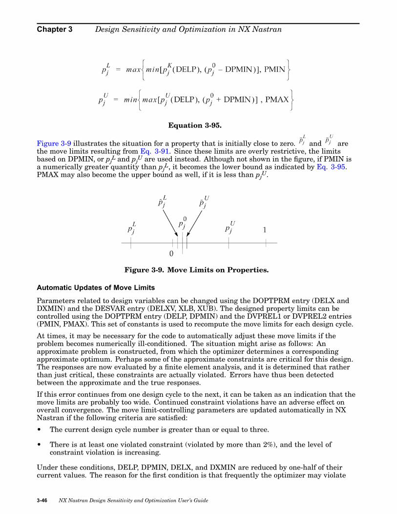
Chapter 3 Design Sensitivity and Optimization in NX Nastran
Equation 3-95.
Figure 3-9 illustrates the situation for a property that is initially close to zero. and arethe move limits resulting from Eq. 3-91. Since these limits are overly restrictive, the limitsbased on DPMIN, or pj
L and pjU are used instead. Although not shown in the figure, if PMIN is
a numerically greater quantity than pjL, it becomes the lower bound as indicated by Eq. 3-95.
PMAX may also become the upper bound as well, if it is less than pjU.
Figure 3-9. Move Limits on Properties.
Automatic Updates of Move Limits
Parameters related to design variables can be changed using the DOPTPRM entry (DELX andDXMIN) and the DESVAR entry (DELXV, XLB, XUB). The designed property limits can becontrolled using the DOPTPRM entry (DELP, DPMIN) and the DVPREL1 or DVPREL2 entries(PMIN, PMAX). This set of constants is used to recompute the move limits for each design cycle.
At times, it may be necessary for the code to automatically adjust these move limits if theproblem becomes numerically ill-conditioned. The situation might arise as follows: Anapproximate problem is constructed, from which the optimizer determines a correspondingapproximate optimum. Perhaps some of the approximate constraints are critical for this design.The responses are now evaluated by a finite element analysis, and it is determined that ratherthan just critical, these constraints are actually violated. Errors have thus been detectedbetween the approximate and the true responses.
If this error continues from one design cycle to the next, it can be taken as an indication that themove limits are probably too wide. Continued constraint violations have an adverse effect onoverall convergence. The move limit-controlling parameters are updated automatically in NXNastran if the following criteria are satisfied:
• The current design cycle number is greater than or equal to three.
• There is at least one violated constraint (violated by more than 2%), and the level ofconstraint violation is increasing.
Under these conditions, DELP, DPMIN, DELX, and DXMIN are reduced by one-half of theircurrent values. The reason for the first condition is that frequently the optimizer may violate
3-46 NX Nastran Design Sensitivity and Optimization User’s Guide

Design Sensitivity and Optimization in NX Nastran
the constraints somewhat as it makes favorable gains in the objective function in the first fewcycles. However, if this condition continues, it may indicate that the problem is becomingill-conditioned as a result of excessive move limits. A corresponding User Warning Message isprinted as notification that this update has occurred (see Output Features and Interpretation).If the job is to be restarted, an updated DOPTPRM entry with the new move limits should beincluded in the restart deck.
Under no conditions does an update increase the move limits. The only type of update isa reduction by one-half. The move limits cannot be increased again unless the engineerintervenes and manually changes them.
Implementation of Move Limits
Move limits on independent design variables are applied directly. Since the optimizer will neverpropose a value for a design variable outside of its bounds, the lower and upper move limitscomputed from Eq. 3-89, Eq. 3-92, and Eq. 3-94 are simply input directly to the optimizer.
Move limits on dependent design variables are imposed as equivalent constraints, similarto that of properties in Eq. Eq. 3-96.
Move limits on properties, however, are implemented as equivalent constraints. For the j-thproperty in the design model, the equivalent lower and upper bound constraints are given by
Equation 3-96.
where the lower and upper bounds pjL and pj
U are given by Eq. 3-93 and Eq. 3-95.
Eq. 3-96 is necessary because the optimizer modifies design variables and not properties. Ofcourse, the property values are known from the DVPREL1 and DVPREL2 relations. For anygiven set of design variables, the optimizer can use Eq. 3-96 to determine whether or not thecorresponding properties are within their allowable limits.
Relaxation of Move Limits
Since a small numerical constraint violation is allowed by the optimizer (by default), move limitson properties may not be satisfied with equality at their bounds. This is usually of little concernexcept when the design is at PMIN or PMAX in Eq. 3-95. Occasionally, these bounds might beslightly violated in a numerical sense but usually is of little consequence.
A puzzling situation may occur if the current design is infeasible. If this is the case, theoptimizer’s primary task is to reduce the level of constraint violation to find a feasible solution ifone exists. Since the move limits on properties are implemented as equivalent constraints, theoptimizer does not know the difference between response-type and move limit-type constraints.Thus, by seeking to reduce the level of constraint violation, some of these move limits may beviolated. For initial designs with highly violated constraints, it is not unusual to see analysis
NX Nastran Design Sensitivity and Optimization User’s Guide 3-47

Chapter 3 Design Sensitivity and Optimization in NX Nastran
model properties vary by 25% or 30% even though the move limits may actually only be 20%.This usually does not pose any practical difficulties, but if it does, the initial move limits canalways be reduced accordingly using the DOPTPRM entry. (In rare instances this optimizationfeature may yield a physically meaningless property value (e.g., a negative plate thickness). Inthis case the analysis cannot proceed and a fatal message will be issued. The remedy, should thisoccur, is to restart with a reduced value of DELP on the DOPTPRM entry.)
Using Design Variable Bounds to Enforce Move Limits on Properties.In contrast, the bounds on design variables are always honored by the optimizer. Since thedesign variables are the quantities that the optimizer varies directly (and thus has direct controlover), their bounds are never exceeded. To implement bounds on properties that are criticalfrom a design standpoint, it is recommended that a linear design variable to property relation(DVPREL1) be prescribed if possible with appropriate bounds on the design variable (stated onthe DESVAR entry). Since the design variable bounds are always enforced, the correspondingproperty then never exceeds its lower and upper bounds. (An exception here is with respect todependent design variable bounds, which are always treated as constraints.)
Numerically Identifying the Active and Violated ConstraintsA numerical optimizer must use numerical criteria to judge when a constraint is active andwhen it is violated. These criteria are established using the values of CT and CTMIN, whichappear on the DOPTPRM entry.
These quantities are shown in Figure 3-10 for a single inequality constraint in a simpletwo-design variable space. A constraint is considered active if its numerical value exceeds CT.Once a constraint is active, its gradient is included in the search direction computation. Seeappendix D on numerical optimization for further details. An active constraint may subsequentlybecome inactive if its value falls below CT.
3-48 NX Nastran Design Sensitivity and Optimization User’s Guide

Design Sensitivity and Optimization in NX Nastran
Figure 3-10. Active and Violated Constraints.
The optimizer identifies a constraint as active if its value is greater than CTMIN. Its defaultis 0.003 as is seen in Figure 3-11. Thus, some small constraint violation (three-tenths of onepercent, by default) is tolerated. Note that this establishes a numerical constraint boundary thatis not identical to the exact constraint boundary.
Figure 3-11. CT and CTMIN.
NX Nastran Design Sensitivity and Optimization User’s Guide 3-49

Chapter 3 Design Sensitivity and Optimization in NX Nastran
Optimizer Convergence
Appendix D describes the criteria used to denote convergence at the optimizer level. Rather thanrepeat that discussion here, mention is made instead of those parameters that you can modify toaffect this convergence (although experience here has indicated that there is seldom a need tovary these parameters.) All of these may be changed using the DOPTPRM entry; see Table 1of that entry for a discussion and defaults.
Parameters related to convergence at the optimizer level include the following:
DABOBJ Absolute change in the objective to denote convergence at the optimizer level.
DELOBJ Relative change in the objective function to denote convergence at theoptimizer level. The combination of DABOBJ and DELOBJ is used to identifythe diminishing returns associated with convergence at the optimizer level.
ITMAX Maximum number of iterations allowed within the optimizer (default = 40).This value is provided so that poorly converging problems are caught.
ITRMOP The number of consecutive iterations for which the DABOBJ, DELOBJconvergence criteria must be satisfied before convergence is indicated.
ITRMST The number of consecutive iterations for which the convergence criteria mustbe satisfied to indicate convergence in the sequential linear programmingmethod. This is equivalent to ITRMOP and defines the maximum number ofapproximate linear problems that may be solved.
JTMAX Maximum number of iterations allowed in the sequential linear programmingmethod, used only if METHOD = 2 (see DOPTPRM entry). Its function isequivalent to ITMAX, used for the modified method of feasible directions.
3.4 Convergence TestsSince structural optimization is an iterative process, numerical criteria must be established todetermine when the overall process has converged. There are two levels at which convergenceis tested: the first and lower level is at the optimizer level; the second and higher level is withrespect to the overall design cycles. This section is concerned with design-cycle level convergence.Convergence at the optimizer level is briefly discussed at the end of the previous section and ingreater detail in Numerical Optimization .
The numerical values of all of the convergence criteria discussed in this section can be changedusing the DOPTPRM Bulk Data entry. This entry is optional, though, since defaults for all ofthese quantities has been provided. However, it is recommended that you always check to ensuretheir validity for the problem at hand. The trade-off between analysis cost and acceptable designaccuracy should always be of prime consideration.
3-50 NX Nastran Design Sensitivity and Optimization User’s Guide

Design Sensitivity and Optimization in NX Nastran
Convergence of Design Cycles: Hard and Soft Convergence
Two methods are used to test for convergence with respect to overall design cycles. Thesemethods are denoted as soft convergence and hard convergence. Soft convergence is based onthe results of the approximate optimization, while hard convergence is based on finite elementanalysis results.
Recall that at the outset of each design cycle, a finite element analysis and a sensitivity analysisare performed. The approximate model is then constructed followed by an optimization withrespect to this approximation. Once a corresponding approximate optimum is found, theproposed design is submitted for another finite element analysis to compute the updatedresponses, thus marking the beginning of the next design cycle.
Hard convergence compares the results of this most recent finite element analysis with thosefrom the previous design cycle. Since this test compares the exact results (within the limits ofthe finite element approximations) from two consecutive analyses, the conclusions are said tobe based on hard evidence. Since this test is conclusive, this is the default test for determiningwhether or not to terminate the design-cycle process.
Soft convergence compares the design responses from the approximate optimization with thoseobtained from the previous finite element analysis. This test, although not as conclusive as hardconvergence, is often an acceptable criterion to indicate convergence. For example, if a particularanalysis model has a high solution cost and the optimizer has not changed the design to anylarge degree, it may be permissible to forego the final finite element analysis. The results fromthe previous analysis are probably of sufficient validity for design purposes; therefore, softconvergence may be a preferable and cost effective exit point.
Soft convergence does not terminate the design cycle process unless the parameterSOFTEXIT is explicitly set to ‘YES’. The default for SOFTEXIT is ‘NO’.
These convergence tests are shown in the simplified flowchart of Figure 3-12. On the initialcycle, the hard convergence test is skipped and program flow proceeds directly to the sensitivityanalysis and approximate optimization. Once an approximate optimum is obtained, a softconvergence test is performed to compare these results with the prior finite element analysisresults. However, the design process is stopped only if soft convergence is indicated and theparameter SOFTEXIT has been set to ‘YES’. This test is performed regardless of whether theparameter SOFTEXIT is set to ‘YES’. The printout for each design cycle includes a status reporton the soft convergence test; see Output Features and Interpretation for examples of this output.
NX Nastran Design Sensitivity and Optimization User’s Guide 3-51

Chapter 3 Design Sensitivity and Optimization in NX Nastran
Figure 3-12. Convergence Testing and Program Flow.
If soft convergence has not terminated the design process, a finite element evaluation of the newproposed design is performed followed by constraint evaluation and screening. If the analysisresults are not appreciably different from those of the prior cycle, hard convergence is achieved,and the design cycle process is terminated. If the hard convergence criteria are not satisfied,the design cycle process continues.
Maximum Number of Iterations DESMAX
If neither hard nor soft convergence is achieved, the design process will continue untilconvergence is indicated or until the maximum allowable number of iterations is met. Thisdefault maximum number of iterations is five but can be changed on the DOPTPRM entryusing DESMAX.
The following paragraphs flowchart and discuss the soft and hard convergence decision logic.
Soft Convergence Decision Logic
A schematic of the soft convergence decision logic is shown in Figure 3-13. The result of the testis a true or false value for the logical variable SOFTCV. The design cycle terminates only if
3-52 NX Nastran Design Sensitivity and Optimization User’s Guide

Design Sensitivity and Optimization in NX Nastran
SOFTCV is ‘TRUE’ and the parameter SOFTEXIT is ‘YES’. No other combinations allow softconvergence to halt the design-cycle process.
Figure 3-13. Soft Convergence Decision Logic.
From Figure 3-13 , the first test is a check of the relative and absolute changes in the objective.The definitions of these parameters appear in Table 3-1 along with their default values. Thesevalues may be modified using the DOPTPRM entry and also apply to the hard convergencechecks.
Table 3-1. Convergence Criteria Parameters.Internal Variable Definition Parameters Default
CHGOBJ CONV1 0.001
ACHOBJ CONV2 0.01
CHGPRP CONVPR 0.001
NX Nastran Design Sensitivity and Optimization User’s Guide 3-53

Chapter 3 Design Sensitivity and Optimization in NX Nastran
Table 3-1. Convergence Criteria Parameters.Internal Variable Definition Parameters Default
CHGDV CONVDV 0.001
CONMAX GMAX 0.005
If either of the relative or absolute changes in the objective is satisfied, the next check is to seewhether or not the analysis model properties have changed appreciably. If the changes in theobjective and analysis model properties are negligible, the subsequent check determines if thedesign constraints are satisfied. If these constraints are satisfied, then soft convergence to afeasible design is achieved.
If some of the constraints are still not satisfied, a check on the change in design variables isperformed. The conclusion here is that if the design variables, properties, and objective functionare unchanged by the optimizer, then convergence is indicated although to an infeasible design.Since the optimizer cannot make any further progress, an additional finite element analysisis probably unnecessary.
Hard Convergence Decision LogicHard convergence is always used to decide whether or not the design cycle process shouldcontinue, providing that the maximum allowable number of design cycles (DESMAX) is not yetreached. The satisfaction of hard convergence is always sufficient to stop the design process.
A flowchart of these criteria is shown in Figure 3-14 with the corresponding definitions of theterms appearing previously in Table 3-1. Even though this test may indicate convergence, notethat one of three possible conclusions may be reached.
3-54 NX Nastran Design Sensitivity and Optimization User’s Guide

Design Sensitivity and Optimization in NX Nastran
Figure 3-14. Hard Convergence Decision Logic.
As with soft convergence, the first check is with respect to the relative and absolute changesin the objective function. The reasoning behind the application of an ‘OR’ test is based on aconsideration of the objective function magnitude. If the objective is large, such as the weight ofa heavy machine part in kilograms, converging to within a plus or minus range of ten kilogramsis probably quite sufficient. Forcing convergence to within a fraction of a kilogram may bemeaningless as well as expensive. On the other hand, there are situations where the objectivefunction is a very small number (e.g., minimization of the difference between analysis andtest results). For such cases, minimization of the absolute change may be more meaningfulthan the relative change.
In Version 66 of MSC.Nastran, a logical ‘AND’ had been used for the objective functiontest, which often proved to be overly restrictive.
If the objective has not changed appreciably in either an absolute or a relative sense, a check isperformed to ensure that the maximum constraint value is less than its maximum allowable. Ifthis criterion is satisfied, then hard convergence is achieved. However, you should check to see ifthe relative changes in properties CHGPRP or the relative changes in design variables CHGDVare satisfied. If they were met, then the design process has converged to a unique design. Ifnot, a nonunique design may have been found.
NX Nastran Design Sensitivity and Optimization User’s Guide 3-55

Chapter 3 Design Sensitivity and Optimization in NX Nastran
Convergence to a Nonunique Optimum.
From a design perspective, convergence to a nonunique design is extremely useful information.This would indicate that the optimum properties could be modified by the engineer withcorrespondingly little change in the objective function and/or constraints. (In other words, theoptimal design exhibits low sensitivity with respect to changes in the design variables.) A designspace of this type is shown in Figure 3-15 where contours of the objective and active constraintboundary have similar curvatures in the region of the optimum. In situations such as these,the design may be modified to take advantage of available sheet metal gauges or tube sizeswithout violating the active constraint(s) and with correspondingly little change to the optimumobjective. Of course, any proposed changes should be subjected to an analysis and the resultschecked carefully to ensure that other performance constraints are not violated.
Figure 3-15. Nonunique Optimum.
Returning to the hard convergence decision logic of Figure 3-14 , note that the code only checksthe relative changes in properties and design variables if the limit on the maximum constraintvalue is not satisfied. The purpose of this check is to determine whether the design is changingfor the case of violated constraints. If the design is still varying, we are justified in continuingoptimization in order to try to overcome the constraint violation(s). However, if the design is notchanging, then we are at a point in the design space that represents a best compromise solutionamong the violated constraints. This situation is shown in Figure 3-16 where the optimal designis the one that minimizes the sum of the constraint violation.
3-56 NX Nastran Design Sensitivity and Optimization User’s Guide

Design Sensitivity and Optimization in NX Nastran
Figure 3-16. Design Space, No Feasible Solutions.
Given the implications of hard convergence, a careful review of the output is advised in orderto determine which convergence conditions have been met. Just because the process has beenterminated does not necessarily imply that a unique, feasible design has been found.
Caution: Always check and confirm the conditions under which convergence is achieved.
NX Nastran Design Sensitivity and Optimization User’s Guide 3-57


Chapter
4 Input Data
• File Management Section, Executive Control
• Case Control Section
• Bulk Data Entries
• Parameters for Design Sensitivity and Optimization
NX Nastran Design Sensitivity and Optimization User’s Guide 4-1

Chapter 4 Input Data
This chapter describes all Executive Control, Case Control, Bulk Data, and parameterrequirements for design sensitivity and optimization. These various input formats enable thefollowing:
1. Specification of the applicable analysis discipline(s).
2. Definition of the design model.
3. Overrides of the optimizer’s internal parameters.
4. Control of the program flow and results output.
Use of the material in this chapter is covered in Design Modeling for Sensitivity andOptimization, and in Example Problems.
4.1 File Management Section, Executive Control
The NASTRAN Statement
Starting with NX Nastran 5, there is an alternative optimization capability available. Thisoption UGS-ADS, as opposed to DOT which is the default optimizer, can be selected by settingsystem cell 425 (ADSOPT) to 1. Thus, to optimize using UGS-ADS, the following statementshould be inserted in the data file:
NASTRAN … ADSOPT = 1 …
or
NASTRAN … SYSTEM(425) = 1 …
Alternatively, this system cell modification can be done through the Runtime Configuration (RC)files or within the DMAP before invoking the optimization module (DOM9). If system cell 425 isleft at the default value of 0, the program will proceed with the use of the DOT optimizer.
Solution 200
In design sensitivity and optimization, the only required Executive Control statement is theSOL statement:
SOL 200
This states that subDMAP DESOPT is to be invoked, which is the main subDMAP for designsensitivity and optimization. The following section lists the supported analysis types in Solution200; these are chosen using the Case Control command, ANALYSIS.
Solution Sequences 108, 111, and 112 had previously supported dynamic responsesensitivities. This capability has been moved from these solution sequences to Solution200.
Shape Optimization and the File Management SectionFile Management Section statements are required in shape optimization for the direct input ofshapes method. This approach DBLOCATEs a set of displacement vector data from a databaseand uses this data to generate a set of shape basis vectors for design optimization. The followingstatements must be used:
4-2 NX Nastran Design Sensitivity and Optimization User’s Guide

Input Data
ssign f1 = ’file.MASTER’dblocate datablk=(ug/ugd,geom1/geom1d,geom2/geom2d), logical=f1
The filename file.MASTER is the name of the database for the auxiliary model analysis. Thefilename “file” is arbitrary. The UG, GEOM1, and GEOM2 data blocks must be DBLOCATEdand renamed to UGD, GEOM1D, and GEOM2D, respectively. These new names cannot bechanged since the code looks for the data in these locations explicitly. See Relating DesignVariables to Shape Changes and Shape Optimization of a Culvert for a discussion of, andexamples using, this method.
4.2 Case Control SectionIn NX Nastran analysis, the Case Control Section is used to specify the applied loads, boundaryconditions, and subcases, and to request the form and type of analysis output. The additions tothe Case Control for design optimization are few and do not require any modification of the CaseControl commands already required for analysis.
Case Control commands for design sensitivity and optimization are associated with the followingfour tasks:
• Analysis discipline definition.
• Design model definition.
• Design response characterization.
• Shape basis vector computation.
This section discusses each of these tasks individually.
Analysis Discipline Definition
Design optimization in NX Nastran is multidisciplinary: a number of different analyses may beperformed in Solution 200, and the results used simultaneously in optimization.
The analysis types are defined on a subcase basis using the ANALYSIS Case Control command.It can be set to any of the following values:
The following are a few Case Control issues to be aware of when using the ANALYSIS command.
• If ANALYSIS is specified above the subcase level, all subsequent subcases apply to thatanalysis type until redefined in a later subcase.
NX Nastran Design Sensitivity and Optimization User’s Guide 4-3

Chapter 4 Input Data
• The buckling subcase defined by ANALYSIS = BUCK refers to the first STATICS subcase.
• Multiple boundary conditions may be used in Solution 200 for ANALYSIS = STATICS.
• Limited multiple boundary condition support exists for ANALYSIS = MODES. A normalmodes subcase can have its own unique set of boundary conditions, but only one normalmodes subcase can exist in a Solution 200 run.
Design Model Definition
The design model definition process in Case Control includes identification of the design objectivefunction and the design constraint sets.
Design Objective Identification
The design objective is identified in Case Control with the command:
Equation 4-1.
where n is the set identification of a design response on either a DRESP1 or DRESP2 Bulk Dataentry. This response must be a single, scalar quantity.
A DESOBJ entry appearing above the subcase level identifies a “global” response. Weight andvolume are typical examples of global responses. DESOBJ can also be used at the subcase level ifthe design goal is to minimize or maximize a subcase-dependent response.
Design Constraint Identification
Design constraint sets are identified in Case Control by the following commands:DESGLB = nDESSUB = n
where n is the set identification number of a DCONSTR or a DCONADD Bulk Data entry.
DESGLB is used above the subcase level to define a subcase-independent constraint set. Weightand volume are subcase-independent responses, as are DRESP2 responses that are not functionsof DRESP1 responses (e.g., DRESP2s that are functions of design variables, table constants,and grid coordinates only).
DESSUB defines subcase-dependent constraint sets at the subcase level. A DESSUB commandremains in effect until replaced with a new DESSUB in a subsequent subcase.
The overall design constraint definition process is:
1. Identify design responses in the Bulk Data using DRESP1 and/or DRESP2 entries.
2. Impose limits on these responses using DCONSTR Bulk Data entries.
3. Combine these DCONSTR sets, if desired, using DCONADD Bulk Data entries.
4. Identify the DCONSTR/DCONADD set identification numbers in Case Control usingDESGLB for globally-applied constraints and DESSUB for subcase-dependent constraints.
4-4 NX Nastran Design Sensitivity and Optimization User’s Guide

Input Data
Design Response CharacterizationStrictly speaking, Case Control output requests are unnecessary in design sensitivity andoptimization. In a number of instances they can, however, be quite useful.
Data Recovery in Solution 200Solution 200 builds its own internal Case Control for data recovery based on the list of DRESP1responses identified in the design model. This provision ensures that all necessary data recoveryis always performed for design sensitivity and optimization. However, if you want to view NXNastran results, Case Control output requests are necessary. The frequency of this output withrespect to design cycle number is controlled by the Bulk Data parameter NASPRT.
Case Control and Design ResponsesCase Control output commands can often be used to resolve design response ambiguities. Forexample, element stresses can be output using either von Mises or maximum shear. (Theambiguity arises since both share the same plot code ID referenced on the DRESP1 entry. Seethe NX Nastran Quick Reference Guide for a list of these plot codes.) The form identified in CaseControl is taken as the representation for design sensitivity and optimization. For example,
STRESS( VONMISES ) = 15 (von Mises stresses used for analysis and optimization)STRESS( SHEAR ) = 15 (maximum shear stresses used for analysis and optimization)
If left unspecified, the defaults will be used (which in this case, is the von Mises representation).See the NX Nastran Quick Reference Guide for defaults.
Dynamic responses can be computed using either a real/imaginary or a magnitude/phase form.Here again, Case Control can be used to define the output representation. For example,
STRAIN( IMAG ) = ALL (real/imaginary form for analysis and optimization)STRAIN( PHASE ) = ALL (magnitude/phase form for analysis and optimization)
Output Frequencies and Output Time StepsIn design optimization, design responses in dynamic analysis are computed for all outputfrequencies (ANALYSIS = DFREQ or MFREQ) and time steps (ANALYSIS = MTRAN). Thiscan lead to a huge amount of data. Case Control can be used to limit this output and savecomputational resources by defining output sets with
OFREQ = nOTIME = m
where n and m are frequency and time sets, respectively.
Design responses will only be computed for the frequencies and/or time steps identified in theabove sets.
Shape Basis Vector ComputationAdditions to Case Control for shape optimization are only necessary when using the analyticboundary shapes method.
Recall from Relating Design Variables to Shape Changes, that the analytic boundary shapesapproach uses additional Bulk Data Sections to describe the auxiliary boundary models. Each ofthese additional sections must have a corresponding Case Control.
NX Nastran Design Sensitivity and Optimization User’s Guide 4-5
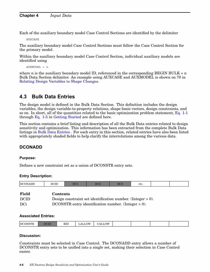
Chapter 4 Input Data
Each of the auxiliary boundary model Case Control Sections are identified by the delimiter
AUXCASE
The auxiliary boundary model Case Control Sections must follow the Case Control Section forthe primary model.
Within the auxiliary boundary model Case Control Section, individual auxiliary models areidentified using
AUXMODEL = n
where n is the auxiliary boundary model ID, referenced in the corresponding BEGIN BULK = nBulk Data Section delimiter. An example using AUXCASE and AUXMODEL is shown on 70 inRelating Design Variables to Shape Changes.
4.3 Bulk Data EntriesThe design model is defined in the Bulk Data Section. This definition includes the designvariables, the design variable-to-property relations, shape basis vectors, design constraints, andso on. In short, all of the quantities related to the basic optimization problem statement, Eq. 1-1through Eq. 1-5 in Getting Started are defined here.
This section contains a brief listing and description of all the Bulk Data entries related to designsensitivity and optimization. This information has been extracted from the complete Bulk Datalistings in Bulk Data Entries . For each entry in this section, related entries have also been listedwith appropriately shaded fields to help clarify the interrelations among the various data.
DCONADD
Purpose:
Defines a new constraint set as a union of DCONSTR entry sets.
Entry Description:
DCONADD DCID DC1 DC2 DC3 etc.
Field ContentsDCID Design constraint set identification number. (Integer > 0).DCi DCONSTR entry identification number. (Integer > 0).
Associated Entries:
DCONSTR DCID RID LALLOW UALLOW
Discussion:
Constraints must be selected in Case Control. The DCONADD entry allows a number ofDCONSTR entry sets to be unified into a single set, making their selection in Case Controleasier.
4-6 NX Nastran Design Sensitivity and Optimization User’s Guide

Input Data
DCONSTR
Purpose:
Places limits on a design response. When selected in Case Control by either DESGLB orDESSUB, the DCONSTR sets define the design constraints.
Entry Description:
DCONSTR DCID RID LALLOW UALLOW
Field ContentsDCID Design constraint set identification number (Integer > 0).RID DRESPi entry identification number (Integer > 0).LALLOW Lower bound on the response quantity (Real, Default = -1.0E20).UALLOW Upper bound on the response quantity (Real, Default = 1.0E20).
Associated Entries:
The DRESP1 and DRESP2 entries identify responses that may be constrained.
DRESP1 ID LABEL RTYPE PTYPE REGION ATTA ATTB ATT1
ATT2 -etc.-
DRESP2 ID LABEL EQID REGION
“DESVAR” DVID1 DVID2 -etc.-
“DTABLE” LABL1 LABL2 -etc.-
“DRESP1" NR1 NR2 -etc.-
“DNODE” G1 C1 G2 C2 -etc.-
The DCONADD entry can be used to form the union of a number of DCONSTR sets.
DCONADD DCID DC1 DC2 DC3 -etc.-
Discussion:
During the optimization process, material may be removed from and/or added to the structureto achieve the optimum objective. As this occurs, the response of the structure to the appliedloads changes. Member stresses, joint displacements, natural frequencies, etc., are alteredby the changes that the optimizer is making.
It is important, then, to place bounds on the structural responses so that the optimized structureresponds in a manner that is acceptable to the designer. For example, it is common to placeupper and lower bounds on the member stresses so that the maximum allowable stresses arenot exceeded. Joint displacement, buckling load factors, and natural frequencies might also bebounded. When a bound is placed on a structural response, this condition is called a constraint.Both first and second-level responses may be constrained.
To constrain a given response quantity, a DCONSTR (Design CONSTRaint) entry is used. Thisentry, in turn, points to a specific response ID identified on either a DRESP1 or a DRESP2 BulkData entry. Note that the DCONSTR entry serves only to place bounds on a response defined
NX Nastran Design Sensitivity and Optimization User’s Guide 4-7

Chapter 4 Input Data
elsewhere in the design model data. These bounds are used to construct normalized constraintsfor use by the optimizer as discussed in Defining the Constraints .
DCONSTR entry sets (or the DCONADD union of these sets) must be selected in the CaseControl Section to complete the constraint definition process. The Case Control commandDESGLB is used to identify subcase-independent constraints (global constraints), while theDESSUB Case Control command is used to select subcase-dependent constraint sets.
DEQATN
Purpose:
Defines equations for use in synthetic relations. These equations can be used to define eithersecond-level responses or second-level design variable-to-property relations.
Entry Description:
DEQATN EQID EQUATION
EQUATION (Cont.)
Field ContentsEQID Unique equation identification number. (Integer > 0).EQUATION Equation(s) (Character).
Associated Entries:
The equation ID may be referenced in connection with a second-level response on a DRESP2entry or in the definition of a synthetic property relation on a DVPREL2 entry.
DRESP2 ID LABEL EQID REGION
“DESVAR” DVID1 DVID2 -etc.-
“DTABLE” LABL1 LABL2 -etc.-
“DRESP1" NR1 NR2 -etc.-
“DNODE” G1 C1 G2 C2 -etc.-
DVPREL2 ID TYPE PID FID PMIN PMAX EQID
“DESVAR” DVID1 DVID2 DVID3 -etc.-
“DTABLE” LABL1 LABL2 LABL3 -etc.-
Discussion:
A unique feature of NX Nastran design sensitivity and optimization is that it allows the engineerto create new response quantities and nonlinear design variable-to-property relations. Thisis accomplished by defining equations much like the function definition procedure of manyprogramming languages.
The DEQATN entry is used to specify a single equation or a set of nested equations. The syntaxof the expressions follows the FORTRAN language standard except that all arguments areassumed to be real numbers (no integers). Intrinsic functions may also be used.
4-8 NX Nastran Design Sensitivity and Optimization User’s Guide

Input Data
The equation input arguments are formal arguments that are defined at runtime. The DRESP2entry for responses and the DVPREL2 entry for design variable-to-property relations specify theinput, or actual, arguments to the appropriate DEQATN entry.
If nested equations are used on a DEQATN entry, the return value is determined from thelast equation on the entry.
A nested form of equation definition may also be used. Multiple equations can be specified on asingle DEQATN entry with the input to the latter equations based on the results of the previousequations. The return value of the function call is the last equation in the DEQATN entry. Theargument list, however, must contain all of the formal arguments used by all equations onthe entry. For more details, see Relating Design Variables to Properties and Identifying theDesign Responses .
DESVAR
Purpose:
Defines the design variables to be used in design sensitivity and optimization. Design sensitivityanalysis computes the rates of change of design responses with respect to changes in the designvariables. In design optimization, the set of design variables are the quantities modified by theoptimizer in the search for an improved design.
Entry Description:
DESVAR ID LABEL XINIT XLB XUB DELXV
Field ContentsID Unique design variable identification number. (Integer > 0).LABEL User-supplied name for printing purposes. (Character).XINIT Initial value. (Real, XLB ≤ XINIT ≤ XUB).XLB Lower bound. (Real, default = -1 .0E+20).XUB Upper bound. (Real, default = +1 .0E+20).
DELXV Move limit for the design variable during approximate optimization. (Real >0.0).
Associated Entries:
Design variables may be related to properties on DVPREL1 or DVPREL2 entries, related tochanges in shape using DVBSHAP, DVGRID, or DVSHAP entries, linked using DLINK entries orinput to user-defined responses on the DRESP2 entry.
DVPREL1 ID TYPE PID FID PMIN PMAX C0
DVID1 COEF1 DVID2 COEF2 DVID3 -etc.-
DVPREL2 ID TYPE PID FID PMIN PMAX EQID
“DESVAR” DVID1 DVID2 DVID3 -etc.-
“DTABLE” LABL1 LABL2 LABL3 -etc.-
NX Nastran Design Sensitivity and Optimization User’s Guide 4-9

Chapter 4 Input Data
DVBSHAP DVID AUXMOD COL1 SF1 COL2 SF2 COL3 SF3
DVGRID DVID GID CID COEFF N1 N2 N3
DVSHAP DVID COL1 SF1 COL2 SF2 COL3 SF3
DLINK ID DDVID C0 CMULT IDV1 C1 IDV2 C2
IDV3 C3 -etc.-
DRESP2 ID LABEL EQID REGION
“DESVAR” DVID1 DVID2 -etc.-
“DTABLE” LABL1 LABL2 -etc.-
“DRESP1" NR1 NR2 -etc.-
“DNODE” G1 C1 G2 C2 -etc.-
Discussion:
In design optimization, structural properties are changed in order to determine the optimalvalue of the objective function. To accomplish this, the optimizer varies the design variables. Notonly must design variables be defined, but they also must be functionally related to analysismodel properties and/or changes in structural shapes. The DESVAR entry is used to define anindividual design variable. Design variables may be defined as members of independent anddependent sets using DLINK Bulk Data entries, if desired.
DLINK
Purpose:
Imposes a linear relationship among the design variables. The set of all DLINK entries partitionsthe design variables into an independent set and a dependent set.
Entry Description:
DLINK ID DDVID CO CMULT IDV1 C1 IDV2 C2
IDV3 C3 -etc.-
Field ContentsID Unique entry identifier. (Integer > 0).DDVID Dependent design variable identification number. (Integer > 0).C0 Constant term. (Real, default = 0.0).CMULT Constant multiplier. (Real, default = 1.0).IDVi Independent design variable identification number. (Integer > 0).Ci Coefficient i (corresponding to IDVi). (Real).
Associated Entries:
Design variables are identified in DLINK relations by their IDs (both independent anddependent variables).
4-10 NX Nastran Design Sensitivity and Optimization User’s Guide

Input Data
DESVAR ID LABEL XINIT XLB XUB DELXV
Discussion:
A DLINK entry specifies a design variable relationship of the form:
Equation 4-2.
where:
xD = dependent design variableco = constantci = constant multiplying coefficientxi = independent design variables
Design variable linking can be used to ensure structural symmetry, unify sizing changes acrossproperty groups, etc. The efficiency of the design process is usually improved if the numberof independent design variables can be kept to a minimum. Placing a design variable in thedependent set using a DLINK entry removes it from the independent set.
DOPTPRM
Purpose:
Overrides default values of parameters used in design optimization.
Entry Description:
DOPTPRM PARAM1 VAL1 PARAM2 VAL2 PARAM3 VAL3 PARAM4 VAL4
PARAM5 VAL5 -etc.-
Field Contents
PARAMi Name of the design optimization parameter. For allowable names, see theDOPTPRM listing in Bulk Data Entries (Character).
VALi Value of the parameter. (Real or Integer, see the DOPTPRM listing in BulkData Entries ).
Associated Entries:
There are no directly associated entries.
Discussion:
There are numerous parameters that control various aspects of the optimization process itself.While all of these parameters have defaults (the DOPTPRM entry is optional), the defaults canbe changed using the DOPTPRM entry. See also the Bulk Data listing in Bulk Data Entries as itcontains the complete list of all optimization parameters that may be changed. Following is anoverview of the various parameters, grouped according to their functionality.
NX Nastran Design Sensitivity and Optimization User’s Guide 4-11
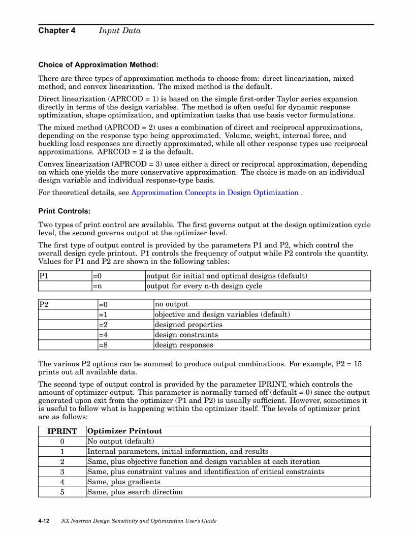
Chapter 4 Input Data
Choice of Approximation Method:
There are three types of approximation methods to choose from: direct linearization, mixedmethod, and convex linearization. The mixed method is the default.
Direct linearization (APRCOD = 1) is based on the simple first-order Taylor series expansiondirectly in terms of the design variables. The method is often useful for dynamic responseoptimization, shape optimization, and optimization tasks that use basis vector formulations.
The mixed method (APRCOD = 2) uses a combination of direct and reciprocal approximations,depending on the response type being approximated. Volume, weight, internal force, andbuckling load responses are directly approximated, while all other response types use reciprocalapproximations. APRCOD = 2 is the default.
Convex linearization (APRCOD = 3) uses either a direct or reciprocal approximation, dependingon which one yields the more conservative approximation. The choice is made on an individualdesign variable and individual response-type basis.
For theoretical details, see Approximation Concepts in Design Optimization .
Print Controls:
Two types of print control are available. The first governs output at the design optimization cyclelevel, the second governs output at the optimizer level.
The first type of output control is provided by the parameters P1 and P2, which control theoverall design cycle printout. P1 controls the frequency of output while P2 controls the quantity.Values for P1 and P2 are shown in the following tables:
P1 =0 output for initial and optimal designs (default)=n output for every n-th design cycle
P2 =0 no output=1 objective and design variables (default)=2 designed properties=4 design constraints=8 design responses
The various P2 options can be summed to produce output combinations. For example, P2 = 15prints out all available data.
The second type of output control is provided by the parameter IPRINT, which controls theamount of optimizer output. This parameter is normally turned off (default = 0) since the outputgenerated upon exit from the optimizer (P1 and P2) is usually sufficient. However, sometimes itis useful to follow what is happening within the optimizer itself. The levels of optimizer printare as follows:
IPRINT Optimizer Printout0 No output (default)1 Internal parameters, initial information, and results2 Same, plus objective function and design variables at each iteration3 Same, plus constraint values and identification of critical constraints4 Same, plus gradients5 Same, plus search direction
4-12 NX Nastran Design Sensitivity and Optimization User’s Guide

Input Data
IPRINT Optimizer Printout6 Same, plus scaling factors and miscellaneous search information7 Same, plus one-dimensional search information
Maximum Number of Design Cycles:
The optimization process is iterative since the optimizer obtains data about the design spacefrom approximations. The approximate model, constructed based on a detailed finite elementanalysis, is used by the optimizer to find an approximate optimum. This design is resubmittedfor another finite element analysis followed by another approximate optimization. This processis repeated until convergence with respect to these overall design cycles is reached. The defaultmaximum number of such cycles is five unless the problem converges before then. Usually, anear-optimum design is found by this point; however, more cycles are often necessary. If themaximum number of design cycles is reached before convergence is achieved, the problem canalways be restarted from the last design (see Restarts in Design Optimization).
Move Limits on the Approximate Optimization:
As the optimizer modifies the design variables, the structure’s properties and/or shape will varydepending on the design model description. As discussed in Section 3.3, Optimization withRespect to Approximate Models, move limits need to be placed on the approximate subproblemfor efficiency reasons. These move limits are imposed with respect to analysis model propertiesas well as design variables. They can be changed from their defaults by modifying DELP andDPMIN for properties, and DELX, DELXV and DXMIN for design variables.
Convergence Criteria:
Convergence at the Design Cycle LevelThe parameters CONV1, CONV2, GMAX, CONVDV, and CONVPR are used to test for overalldesign cycle convergence. These parameters are used in connection with tests for both hardand soft convergence. Convergence Tests , describes the types of convergence testing as wellas the convergence decision logic.
Soft ConvergenceSoft convergence compares the results of the approximate optimization with the results of thefinite element analysis performed at the beginning of the design cycle. Soft convergence isnot sufficient to terminate the design cycle iterations unless the parameter SOFTEXIT is setto YES. NO is the default.
Hard ConvergenceHard convergence testing compares the analysis results of current design cycle with those ofthe previous cycle. This test is a more conclusive test of convergence since it is based on hardevidence. Hard convergence will always terminate the design cycle process.
Convergence at the Optimizer LevelConvergence at the optimizer level can also be controlled using the DOPTPRM entry. Parametersthat can be changed include DABOBJ, DELOBJ, ITMAX, ITRMOP, ITRMST, and JTMAX.
Finite Difference Step Sizes:
Design sensitivity coefficients are computed in NX Nastran using a semianalytic approach,as explained in Design Sensitivity Analysis .
NX Nastran Design Sensitivity and Optimization User’s Guide 4-13
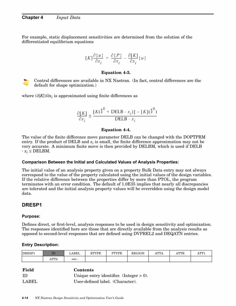
Chapter 4 Input Data
For example, static displacement sensitivities are determined from the solution of thedifferentiated equilibrium equations
Equation 4-3.
Central differences are available in NX Nastran. (In fact, central differences are thedefault for shape optimization.)
where (∂[K])/∂xi is approximated using finite differences as
Equation 4-4.
The value of the finite difference move parameter DELB can be changed with the DOPTPRMentry. If the product of DELB and xi is small, the finite difference approximation may not bevery accurate. A minimum finite move is then provided by DELBM, which is used if DELB· xi ≤ DELBM.
Comparison Between the Initial and Calculated Values of Analysis Properties:
The initial value of an analysis property given on a property Bulk Data entry may not alwayscorrespond to the value of the property calculated using the initial values of the design variables.If the relative difference between the properties differ by more than PTOL, the programterminates with an error condition. The default of 1.0E35 implies that nearly all discrepanciesare tolerated and the initial analysis property values will be overridden using the design modeldata.
DRESP1
Purpose:
Defines direct, or first-level, analysis responses to be used in design sensitivity and optimization.The responses identified here are those that are directly available from the analysis results asopposed to second-level responses that are defined using DVPREL2 and DEQATN entries.
Entry Description:
DRESP1 ID LABEL RTYPE PTYPE REGION ATTA ATTB ATT1
ATT2 -etc.-
Field ContentsID Unique entry identifier. (Integer > 0).LABEL User-defined label. (Character).
4-14 NX Nastran Design Sensitivity and Optimization User’s Guide

Input Data
Field Contents
RTYPE Response type. See DRESP1 listing in Commonly Used Commandsfor Design Optimization . (Character).
PTYPE
Element flag (PTYPE = “ELEM”) or property entry name. Used withelement type responses (stress, strain, force, etc.) to identify theproperty type, since property entry IDs are not unique across propertytypes. (Character: “ELEM,” “PBAR,” “PSHELL,” etc.).
REGION Region identifier for constraint screening. (Integer > 0).
ATTA, ATTB, ATTi Response attributes. See DRESP1 listing in Commonly UsedCommands for Design Optimization . (Integer > 0 or Real or blank).
Associated Entries:
A response identified on a DRESP1 entry may be used either as a constraint or an objective. Theresponse is identified by its ID number on DCONSTR entries.
DCONSTR DCID RID LALLOW UALLOW
A DRESP1 response can also be used as input to synthetic responses defined on DRESP2 entries.It is referenced by its response ID.
DRESP2 ID LABEL EQID REGION
“DESVAR” DVID1 DVID2 -etc.-
“DTABLE” LABL1 LABL2 -etc.-
“DRESP1" NR1 NR2 -etc.-
“DNODE” G1 C1 G2 C2 -etc.-
A first-level response can also be used as an objective if it defines a single, scalar response (e.g.,weight, an eigenvalue, a grid displacement component for a single subcase, and so on). Theobjective is defined in Case Control with the command
Equation 4-5.
where n is the DRESP1 (or DRESP2) entry ID.
Discussion:
Depending on the particular analysis discipline, responses such as displacements, stresses,eigenvalues, etc., may be computed. However, not all of these responses may be of interest froma design optimization standpoint. The DRESP1 entry is used to identify responses that are tobe used in connection with design sensitivity and optimization either as an objective or as aconstraint. These responses may also be used as input to compute a second-level, or synthetic,response on a DRESP2 entry.
An internal Case Control for design sensitivity and optimization is built using the set offirst-level responses. Selecting design responses using DRESP1 entries also ensures that theappropriate data recovery is performed, regardless of Case Control requests the user may havesupplied. Output requests, if desired, still must be specified with the appropriate Case Control
NX Nastran Design Sensitivity and Optimization User’s Guide 4-15

Chapter 4 Input Data
commands; however, this is for postprocessing convenience only and is not a requirement foreither design sensitivity or optimization.
DRESP2
Purpose:
Defines, in conjunction with a DEQATN entry, a second-level response to be used either as anobjective or as a constraint.
Entry Description:
DRESP2 ID LABEL EQID REGION
“DESVAR” DVID1 DVID2 -etc.-
“DTABLE” LABL1 LABL2 -etc.-
“DRESP1" NR1 NR2 -etc.-
“DNODE” G1 C1 G2 C2 -etc.-
Field ContentsID Unique identification number. (Integer > 0).LABEL User-defined label. (Character).EQID DEQATN entry identification number. (Integer > 0).REGION Region identifier for constraint screening. (Integer > 0).“DESVAR” Flag indicating DESVAR entry identification numbers. (Character).DVIDi DESVAR entry identification number. (Integer > 0).
“DTABLE” Flag indicating that the labels for the constants in a DTABLE entryfollow. (Character).
LABLj Label for a constant in the DTABLE entry. (Character).“DRESP1" Flag indicating DRESP1 entry identification numbers. (Character).NRk DRESP1 entry identification number. (Integer > 0).
“DNODE” Flag signifying that the following fields are designed grid points.(Character).
Gm Grid point identification number. (Integer > 0).Cm Degree of freedom number of grid point Gm. (1 ≤ Integer ≤ 3).
Associated Entries:
The DCONSTR entry can be used to place bounds on a DRESP2 response using the DRESP2entry ID as a reference:
DCONSTR DCID RID LALLOW UALLOW
The DESOBJ Case Control command can also reference the DRESP2 entry ID:
4-16 NX Nastran Design Sensitivity and Optimization User’s Guide
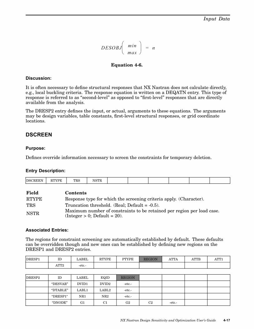
Input Data
Equation 4-6.
Discussion:
It is often necessary to define structural responses that NX Nastran does not calculate directly,e.g., local buckling criteria. The response equation is written on a DEQATN entry. This type ofresponse is referred to as “second-level” as opposed to “first-level” responses that are directlyavailable from the analysis.
The DRESP2 entry defines the input, or actual, arguments to these equations. The argumentsmay be design variables, table constants, first-level structural responses, or grid coordinatelocations.
DSCREEN
Purpose:
Defines override information necessary to screen the constraints for temporary deletion.
Entry Description:
DSCREEN RTYPE TRS NSTR
Field ContentsRTYPE Response type for which the screening criteria apply. (Character).TRS Truncation threshold. (Real; Default = -0.5).
NSTR Maximum number of constraints to be retained per region per load case.(Integer > 0; Default = 20).
Associated Entries:
The regions for constraint screening are automatically established by default. These defaultscan be overridden though and new ones can be established by defining new regions on theDRESP1 and DRESP2 entries.
DRESP1 ID LABEL RTYPE PTYPE REGION ATTA ATTB ATT1
ATT2 -etc.-
DRESP2 ID LABEL EQID REGION
“DESVAR” DVID1 DVID2 -etc.-
“DTABLE” LABL1 LABL2 -etc.-
“DRESP1" NR1 NR2 -etc.-
“DNODE” G1 C1 G2 C2 -etc.-
NX Nastran Design Sensitivity and Optimization User’s Guide 4-17

Chapter 4 Input Data
Discussion:
To reduce the costs associated with the sensitivity analysis and to reduce the size of theoptimization problem, many of the noncritical constraints are dynamically deleted during theoptimization process. Default values of parameters that control the screening process can beoverridden using DSCREEN entries. Since these defaults are often satisfactory, includingDSCREEN entries is often unnecessary.
Constraint DeletionConstraint screening is performed in two stages. In the first step, deletion, the constraintvalues that fall below a certain threshold level are deleted from the constraint set. The defaultthreshold level is –0.5, but this can be overridden by specifying a TRS value on the DSCREENentry. In NX Nastran, the normalized constraints are considered violated if they are positivequantities. The default TRS states that only those constraints that are within 50% of theircritical values are retained.
Constraint RegionalizationThe second step, regionalization, sorts the remaining constraints and retains up to a prescribedmaximum per region per load case. The default region specifications are given on the DSCREENBulk Data entry description. NSTR, or the number of constraints to be retained per region, has adefault value of 20, which again can be overridden.
DTABLE
Purpose:
Defines a table of constants to be used in conjunction with DEQATN equations.
Entry Description:
DTABLE LABL1 VALU1 LABL2 VALU2 LABL3 VALU3 LABL4 VALU4
LABL5 VALU5 LABL6 VALU6 -etc.-
Field ContentsLABLi Label for the constant. (Character).VALUi Value of the constant. (Real).
Associated Entries:
DRESP2 and DVPREL2 entries list the input arguments to equations that define syntheticresponse and property relations, respectively. These input arguments may include tableconstants defined on the DTABLE entry.
DRESP2 ID LABEL EQID REGION
“DESVAR” DVID1 DVID2 -etc.-
“DTABLE” LABL1 LABL2 -etc.-
“DRESP1" NR1 NR2 -etc.-
“DNODE” G1 C1 G2 C2 -etc.-
DVPREL2 ID TYPE PID FID PMIN PMAX EQID
“DESVAR” DVID1 DVID2 DVID3 -etc.-
4-18 NX Nastran Design Sensitivity and Optimization User’s Guide

Input Data
“DTABLE” LABL1 LABL2 LABL3 -etc.-
Discussion:
Constants used in equations can either be “built into” the DEQATN entry when the equation isdefined or passed as arguments. Building-in the values of constants may be inconvenient andcan prevent one equation from easily being used in different contexts.
The DTABLE entry allows these constants to be stored in a table and then used in the equationsas necessary. On the DTABLE entry, a constant is given a name and a value. When the equationargument list is defined on a DVPREL2 or DRESP2 entry, the constant is referenced by its name.
Only one DTABLE entry may appear in the Bulk Data.
DVBSHAP
Purpose:
Defines a shape basis vector as a linear combination of analytic boundary shapes solutionsand assigns a design variable to the result.
Entry Description:
DVBSHAP DVID AUXMOD COL1 SF1 COL2 SF2 COL3 SF3
Field ContentsDVID Design variable identification number of a DESVAR entry. (Integer > 0).AUXMOD Auxiliary model identification number. (Integer > 0).
COLi Load sequence identification number from AUXMODEL Case Controlcommand. (Integer > 0).
SFi Scaling factor for load sequence identification number. (Real; Default =1.0).
Associated Entries:
In shape optimization, shape basis vectors relate the changes in a design variable to changes ingrid locations (see basis vectors in shape optimization, Relating Variables to Shape Changes.)Design variables must first be defined using DESVAR entries.
DESVAR ID LABEL XINIT XLB XUB DELXV
DVGRID
Purpose:
Defines design variable-to-grid coordinate relations for shape sensitivity and optimization.
Entry Description:
DVGRID DVID GID CID COEFF N1 N2 N3
NX Nastran Design Sensitivity and Optimization User’s Guide 4-19

Chapter 4 Input Data
Field ContentsDVID DESVAR entry identification number. (Integer > 0).GID Grid point identification number. (Integer > 0).CID Coordinate system identification number. (Integer ≥ 0; Default = 0).COEFF Multiplier of the vector defined by Ni. (Real; Default = 0.0).
Ni Components of the vector measured in the coordinate system defined byCID. (Real; at least one Ni ≠ 0.0).
Associated Entries:
The DESVAR entry defines a design variable that can be used to describe grid variations as wellas other design relations. The “DNODE” fields on the DRESP2 entry allow the coordinates ofdesigned grids to be used in formulating second-level responses.
DESVAR ID LABEL XINIT XLB XUB DELXV
DRESP2 ID LABEL EQID REGION
“DESVAR” DVID1 DVID2 -etc.-
“DTABLE” LABL1 LABL2 -etc.-
“DRESP1" NR1 NR2 -etc.-
“DNODE” G1 C1 G2 C2 -etc.-
Discussion:
Changes in grid coordinate values are expressed as functions of design variables accordingto the relation
Equation 4-7.
where changes in the i-th grid point are expressed in terms of changes in the j-th design variable.If the number of design variables is less than the number of grid points, this relation is calleda reduced basis formulation. Reduced basis formulations are discussed in Relating DesignVariables to Shape Changes .
The DVGRID entry defines the particular grid point, design variable, and components of each{T}ij vector. Multiple references to the same grid point and design variable pair simply result invectorial addition of the corresponding {T}ij .
Other shape basis vector definition methods utilize DVBSHAP and DVSHAP Bulk Data entries.
DVPREL1
Purpose:
Defines a structural analysis property as a function of a linear combination of design variables.
4-20 NX Nastran Design Sensitivity and Optimization User’s Guide

Input Data
Entry Description:
DVPREL1 ID TYPE PID FID PMIN PMAX C0
DVID1 COEF1 DVID2 COEF2 DVID3 -etc.-
Field ContentsID Unique identification number. (Integer > 0).TYPE Name of a property entry, such as “PBAR”, “PBEAM”, etc. (Character).PID Property entry identification number. (Integer > 0).
FlD Field position of the property entry, or word position in the element propertytable of the analysis model. (Integer ≠ 0.0).
PMIN
Minimum value allowed for this property. If FID references a stressrecovery location, then the default value for PMIN is -1.0+35. PMIN mustbe explicitly set to a negative number for properties that may be less thanzero (for example, field ZO on the PCOMP entry). (Real; Default = 0.001).
PMAX Maximum value allowed for this property. (Real; Default = 1.0E20).C0 Constant term of relation. (Real; Default = 0.0).DVIDi DESVAR entry identification number. (Integer > 0).COEFi Coefficient of linear relation. (Real).
Associated Entries:
Design variables are referenced on DVPREL1 entries by their DESVAR-defined IDs.
DESVAR ID LABEL XINIT XLB XUB DELXV
Discussion:
An analysis model property can be expressed as a linear combination of design variables as
Equation 4-8.
Both independent as well as dependent design variables can appear in this relation (see theDLINK entry). This form is especially useful in the sense that it can be used to express notonly a simple one-to-one correspondence between a design variable and a property, but morecomplex reduced basis formulations as well.
DVPREL2
Purpose:
Defines a structural property by reference to an equation defined on a DEQATN entry.
Entry Description:
DVPREL2 ID TYPE PID FID PMIN PMAX EQID
“DESVAR” DVID1 DVID2 -etc.-
NX Nastran Design Sensitivity and Optimization User’s Guide 4-21

Chapter 4 Input Data
“DTABLE” LABL1 LABL2 -etc.-
Field ContentsID Unique identification number. (Integer > 0).TYPE Name of a property entry, such as PBAR, PBEAM, etc. (Character).PID Property entry identification number. (Integer > 0).FID Field position of the property in the analysis model entry. (Integer ≠ 0.0).
PMIN
Minimum value allowed for this property. If FID references a stress recoverylocation field, then the default value for PMIN is -1.0+35. PMIN must beexplicitly set to a negative number for properties that may be less than zero(for example, field ZO on the PCOMP entry). (Real; Default = 0.001).
PMAX Maximum value allowed for this property. (Real; Default = 1.0E20).EQID DEQATN entry identification number. (Integer > 0).“DESVAR” DESVAR flag. Indicates that the IDs of DESVAR entries follow. (Character).DVIDi DESVAR entry identification number. (Integer > 0).
“DTABLE”DTABLE flag. Indicates that the IDs for the constants in a DTABLE entryfollow. This field may be omitted if there are no constants involved in thisrelation. (Character).
LABi Label for a constant on the DTABLE entry. (Integer > 0).
Associated Entries:
To define a synthetic property relation, the DVPREL2 entry identifies a DEQATN entry anddeclares the design variable (DESVAR) and any necessary table constant (DTABLE) arguments.
DEQATN EQID EQUATION
EQUATION (Cont.)
DESVAR ID LABEL XINIT XLB XUB DELXV
DTABLE LABL1 VALU1 LABL2 VALU2 LABL3 VALU3 LABL4 VALU4
LABL5 VALU5 LABL6 VALU6 -etc.-
Discussion:
For many applications, the linear design variable-to-property relations provided by theDVPREL1 entry may not be sufficient. In these cases, equations may be defined to relate designvariables to properties in a nonlinear fashion. The DVPREL2 entry provides the arguments toan equation defined on a DEQATN entry. These arguments may be design variables defined onDESVAR entries and table constants defined on a DTABLE entry.
Design Sensitivities and Type-2 Properties
Every property defined on a DVPREL2 entry becomes an independently varying propertyinternally in NX Nastran. Design sensitivities are first computed with respect to theseindependently varying properties, and then the chain rule applied to relate these sensitivities tochanges in the design variables. Refer to Design Sensitivity Analysis , for further details.
4-22 NX Nastran Design Sensitivity and Optimization User’s Guide
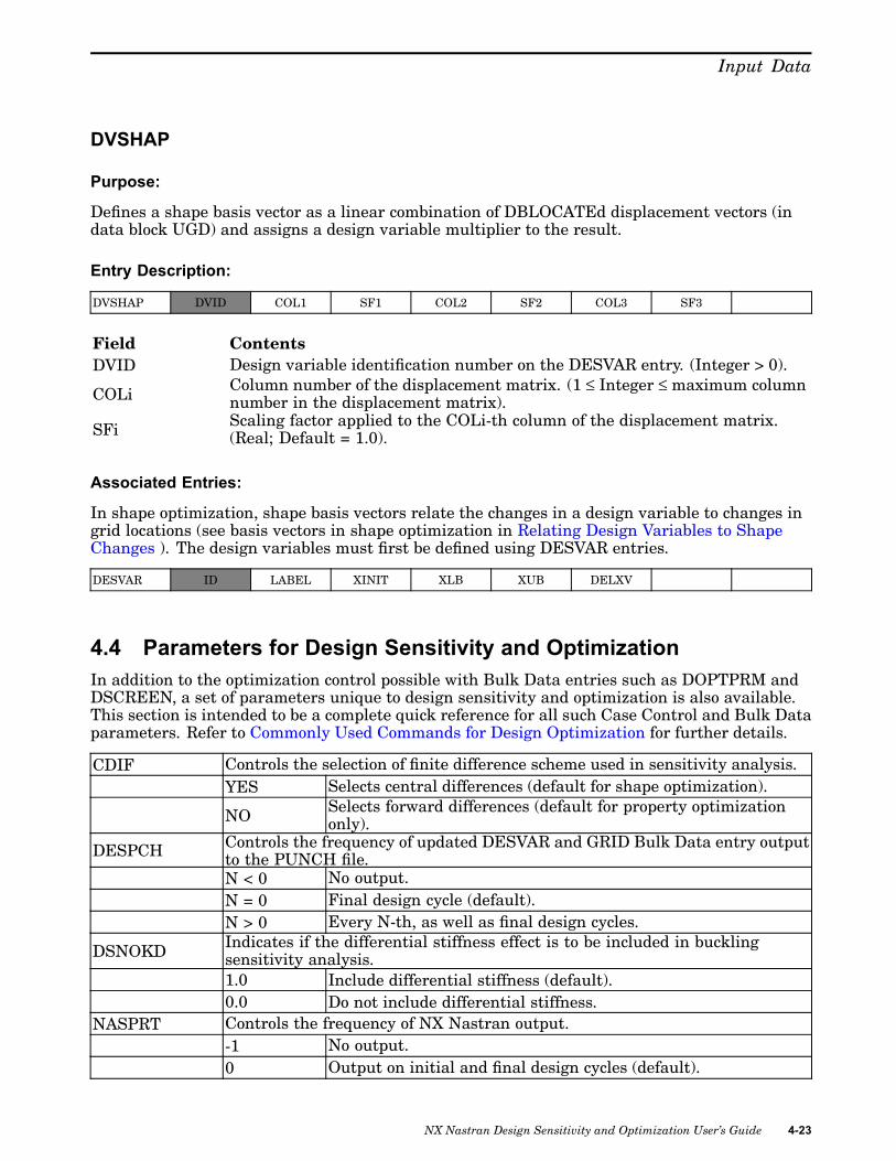
Input Data
DVSHAP
Purpose:
Defines a shape basis vector as a linear combination of DBLOCATEd displacement vectors (indata block UGD) and assigns a design variable multiplier to the result.
Entry Description:
DVSHAP DVID COL1 SF1 COL2 SF2 COL3 SF3
Field ContentsDVID Design variable identification number on the DESVAR entry. (Integer > 0).
COLi Column number of the displacement matrix. (1 ≤ Integer ≤ maximum columnnumber in the displacement matrix).
SFi Scaling factor applied to the COLi-th column of the displacement matrix.(Real; Default = 1.0).
Associated Entries:
In shape optimization, shape basis vectors relate the changes in a design variable to changes ingrid locations (see basis vectors in shape optimization in Relating Design Variables to ShapeChanges ). The design variables must first be defined using DESVAR entries.
DESVAR ID LABEL XINIT XLB XUB DELXV
4.4 Parameters for Design Sensitivity and OptimizationIn addition to the optimization control possible with Bulk Data entries such as DOPTPRM andDSCREEN, a set of parameters unique to design sensitivity and optimization is also available.This section is intended to be a complete quick reference for all such Case Control and Bulk Dataparameters. Refer to Commonly Used Commands for Design Optimization for further details.
CDIF Controls the selection of finite difference scheme used in sensitivity analysis.YES Selects central differences (default for shape optimization).
NO Selects forward differences (default for property optimizationonly).
DESPCH Controls the frequency of updated DESVAR and GRID Bulk Data entry outputto the PUNCH file.N < 0 No output.N = 0 Final design cycle (default).N > 0 Every N-th, as well as final design cycles.
DSNOKD Indicates if the differential stiffness effect is to be included in bucklingsensitivity analysis.1.0 Include differential stiffness (default).0.0 Do not include differential stiffness.
NASPRT Controls the frequency of NX Nastran output.-1 No output.0 Output on initial and final design cycles (default).
NX Nastran Design Sensitivity and Optimization User’s Guide 4-23

Chapter 4 Input Data
N Output every N-th iteration and also prior to exit.OPTEXIT Instructs the program to exit at one of six predetermined exit points.
0 No user-defined exit (default).N > 0 Exit at one of the locations 1 through 7 (1 ≤ N ≤ 7).
SOFTEXIT Determines whether to terminate design cycles if soft convergence is indicated.NO Do not stop if soft convergence is indicated (default).YES Terminate design cycles if soft convergence is achieved.
UPDTBSH Controls the update of the boundary shapes in the analytic boundary shapesmethod for shape optimization.NO Do not update the boundary shapes (default).YES Update the boundary shapes.
Note:Regardless of the value of UPDTBSH, shape basis vectors arestill updated for every design cycle (interpolation to the interiorgrids). UPDTBSH only controls updates on the boundary shapes.
4-24 NX Nastran Design Sensitivity and Optimization User’s Guide

Chapter
5 Output Features andInterpretation
• Output-Controlling Parameters
• Design Optimization Output
• Design Sensitivity Output
NX Nastran Design Sensitivity and Optimization User’s Guide 5-1

Chapter 5 Output Features and Interpretation
Since design optimization is an iterative process, a significant amount of output may begenerated depending on the quantity of data requested for each design cycle and the numberof cycles performed. In design sensitivity and optimization, output may be generated fromthe following four sources:
1. NX Nastran analysis.
2. Design sensitivity analysis.
3. Design optimization (including optimizer output).
4. Convergence tests and design model updates.
Although covered at one place or another in this guide, there are a few parameters that affect thelevel of detail and the frequency of output (for design cycle-dependent data). These parametersare summarized in this chapter in Output-Controlling Parameters.
Following this summary in Design Optimization Output is an output example from a designoptimization problem in the test problem library, supplied with your NX Nastran installationtapes. This example introduces most of the frequently encountered types of design optimizationoutput, within the context of an actual problem. Following in Design Sensitivity Output is asimilar output example for design sensitivity analysis.
5.1 Output-Controlling ParametersBriefly, those quantities that affect either the frequency or level of detail of the output areas follows:
DESPCH Controls the frequency of DESVAR and GRID Bulk Data entry output to thepunch file. The default is for the final design cycle only, but can be changed toevery n-th design cycle (plus the last) with this parameter. See Parameters forDesign Sensitivity and Optimization .
IPRINT Controls the level of printout available directly from the optimizer. Its value,which may range from 0 to 7, is set on the DOPTPRM entry. An increasingvalue provides increasing levels of detail. See the DOPTPRM entry descriptionin Bulk Data Entries .
NASPRT Governs the frequency of NX Nastran analysis results output. Output may berequested for the first and last designs only, the first and every n-th design, orturned off completely with this Bulk Data parameter. See Parameters for DesignSensitivity and Optimization .
OPTEXIT When set to a value of 4 or 7, provides output of the design sensitivity coefficientmatrix DSCM2. This Bulk Data parameter may assume any value from 1 to 7indicating exit at any one of seven predefined locations in the solution sequence.However, only OPTEXIT=4 and 7 generate DSCM2 (design sensitivity coefficient)output. See Parameters for Design Sensitivity and Optimization as well as theSolution 200 flowchart in Solution Sequences .
5-2 NX Nastran Design Sensitivity and Optimization User’s Guide

Output Features and Interpretation
P1 Controls the frequency of design cycle output. By default, initial and finaloptimization summaries are output but can be changed to every n-th cycle usingthis parameter. See the DOPTPRM entry in Bulk Data Entries .
P2 Controls how much design cycle information is output at the intervals determinedby P1. P2 is set using the DOPTPRM entry. See Bulk Data Entries .
5.2 Design Optimization OutputThis section presents design sensitivity and optimization output in the context of one of theexample problems from NX Nastran’s test problem library. One way to present the optimizationoutput would be to include a listing of all of the various output messages and summarieswith a short description of each. However, this approach tends to separate them from theirprocedural context.
Instead, this section traces selected design optimization output from the stiffened plate exampleof Stiffened Plate. This problem is chosen because it contains most of the output commonlyencountered in a typical optimization example. The best approach is for you to locate thisproblem in the test problem library and run it on your installation. The output from the actualproblem can then be referenced while reading this section.
This section was prepared using an IBM/RISC System/6000 workstation. Your resultsmay differ somewhat.
In addition, the Solution 200 flowchart in Solution Sequences might also be useful. Referringto the flowchart will help fix the relationship of the particular output samples to their order inthe design optimization process.
D200X7 OutputThis example problem is presented in Stiffened Plate. If you have not already done so, you maywant to turn to that section first to briefly review the problem set-up.
Assuming you have run this example on your installation and have the output file available, youwill notice the following table appearing shortly after the Bulk Data echo:
----- COMPARISON BETWEEN INPUT PROPERTY VALUES FROM ANALYSIS AND DESIGN MODELS -----
---------------------------------------------------------------------------------------------------------------PROPERTY PROPERTY FIELD ANALYSIS DESIGN LOWER UPPER DIFFERENCE
TYPE ID ID VALUE VALUE BOUND BOUND FLAG---------------------------------------------------------------------------------------------------------------PBAR 3 4 1.440000E-01 1.440000E-01 1.000000E-02 1.000000E+20 NONEPBAR 3 5 1.728000E-04 1.728000E-04 1.000000E-06 1.000000E+20 NONEPBAR 3 6 1.728000E-02 1.728000E-02 1.000000E-06 1.000000E+20 NONEPBAR 3 7 1.745000E-02 1.745000E-02 1.000000E-06 1.000000E+20 NONEPBAR 3 12 6.000000E-02 6.000000E-02 -1.000000E+35 1.000000E+20 NONEPBAR 3 13 6.000000E-01 6.000000E-01 -1.000000E+35 1.000000E+20 NONEPBAR 3 14 6.000000E-02 6.000000E-02 -1.000000E+35 1.000000E+20 NONEPBAR 3 15 -6.000000E-01 -6.000000E-01 -1.000000E+00 1.000000E+20 NONEPBAR 3 16 -6.000000E-02 -6.000000E-02 -1.000000E+00 1.000000E+20 NONEPBAR 3 17 -6.000000E-01 -6.000000E-01 -1.000000E+00 1.000000E+20 NONEPBAR 3 18 -6.000000E-02 -6.000000E-02 -1.000000E+00 1.000000E+20 NONEPBAR 3 19 6.000000E-01 6.000000E-01 -1.000000E+35 1.000000E+20 NONEPSHELL 1 4 1.500000E-01 1.500000E-01 1.000000E-02 1.000000E+20 NONEPSHELL 2 4 2.000000E-01 2.000000E-01 1.000000E-02 1.000000E+20 NONE
1. IF FIELD ID IS LESS THAN ZERO, IT IDENTIFIES THE WORD POSITION OF AN ENTRY IN EPT.
2. IF FIELD ID IS GREATER THAN ZERO, IT IDENTIFIES THE FIELD POSITION ON A PROPERTY BULK DATA ENTRY.
3. THE DIFFERENCE FLAG IS USED TO CHARACTERIZE DIFFERENCES BETWEEN ANALYSIS AND DESIGN MODEL PROPERTIES:
NX Nastran Design Sensitivity and Optimization User’s Guide 5-3

Chapter 5 Output Features and Interpretation
IF THE FLAG IS NONE, THEN THERE IS NO SIGNIFICANT DIFFERENCE BETWEEN THE TWO VALUES.
IF THE FLAG IS WARNING, THEN THE USER IS ADVISED THAT DIFFERENCES EXIST.
IF THE FLAG IS FATAL, THEN THE DIFFERENCES ARE GREATER THAN 1.00000E+35 AND THE RUN WILL BE TERMINATED.
If any of the analysis model properties differs from the design model description, the designmodel will be used to override the analysis model. This table simply reports on any differencesfound and provides notification if this override took place. The design value column containsthe property values computed from the initial design variable values. In this example, nodifferences were found.
The override of the analysis model property values by the design model affords a convenientway of performing a type of rudimentary restart. Simply by changing the initial design variablevalues, you can begin optimization from any point in the design space. (For shape changes,updated GRID entries also need to be included, but these are available from the punch file, if oneor more design cycles have been performed in a previous run.) Once the analysis and designmodels are in agreement, Solution 200 proceeds with an analysis of the model to gather baselineresponse data. A DMAP information message from subDMAP FEA serves notice that a staticanalysis has been initiated:
^^^ DMAP INFORMATION MESSAGE 9051 (FEA) - STATIC ANALYSIS INITIATED. DESIGN CYCLE NUMBER 1
Since this is the first analysis with the parameter NASPRT at its default value of zero, full datarecovery is performed based on Case Control output requests. Since displacements and stresseshave been requested, we see the familiar NX Nastran static analysis output (abbreviated here):
LOAD CONDITION 1 SUBCASE 1D I S P L A C E M E N T V E C T O R
POINT ID. TYPE T1 T2 T3 R1 R2 R310000 G .0 .0 .0 -1.927221E-02 2.565913E-03 .010001 G 1.344270E-03 -1.081616E-04 .0 2.904300E-02 -8.063296E-04 .010002 G 2.957638E-03 -3.128633E-04 .0 3.359672E-02 1.434650E-05 .010003 G 5.187130E-03 -1.556333E-04 .0 2.907712E-02 8.084382E-04 .010004 G 8.248678E-03 1.673541E-03 .0 -1.925253E-02 -2.598804E-03 .010100 G .0 -3.815551E-04 .0 1.309933E-02 -2.005817E-02 .0. . . . . . . .. . . . . . . .. . . . . . . .. . . . . . . .. . . . . . . .
LOAD CONDITION 2 SUBCASE 2S T R E S S E S I N Q U A D R I L A T E R A L E L E M E N T S ( Q U A D 4 )
ELEMENT FIBRE STRESSES IN ELEMENT COORD SYSTEM PRINCIPAL STRESSES (ZERO SHEAR)ID. DISTANCE NORMAL-X NORMAL-Y SHEAR-XY ANGLE MAJOR MINOR VON MISES21 -1.000000E-01 3.894159E+03 4.092442E+03 7.646278E+03 45.3714 1.164022E+04 -3.653620E+03 1.383375E+04
1.000000E-01 3.894159E+03 4.092442E+03 7.646278E+03 45.3714 1.164022E+04 -3.653620E+03 1.383375E+0422 -1.000000E-01 1.656648E+02 2.257865E+03 5.013844E+03 50.8926 6.333576E+03 -3.910047E+03 8.953615E+03
1.000000E-01 1.656648E+02 2.257865E+03 5.013844E+03 50.8926 6.333576E+03 -3.910047E+03 8.953615E+0323 -1.000000E-01 -6.033874E+03 -1.339483E+04 7.341767E+03 31.6875 -1.501711E+03 -1.792699E+04 1.722530E+04
1.000000E-01 -6.033874E+03 -1.339483E+04 7.341767E+03 31.6875 -1.501711E+03 -1.792699E+04 1.722530E+04. . . . . . . . .. . . . . . . . .. . . . . . . . .. . . . . . . . .. . . . . . . . .
This is followed by the DMAP information message:
^^^ DMAP INFORMATION MESSAGE 9052 (FEA) - STATIC ANALYSIS COMPLETED.DESIGN CYCLE NUMBER= 1
If other analyses are performed (normal modes, dynamic response, etc.), similar DMAPinformation messages and data recovery output will follow.
5-4 NX Nastran Design Sensitivity and Optimization User’s Guide

Output Features and Interpretation
With the finite element analysis complete, the code could perform a hard convergence check,were this the second or greater design cycle. Since this is just the first cycle though, DOM12 (themodule that performs the convergence tests) simply reports on the maximum constraint value:
THIS IS THE FIRST ANALYSIS - NO CONVERGENCE CHECK-------------------------------------------------------MAXIMUM VALUE OF CONSTRAINTS : 1.3119E+00
-------------------------------------------------------
See Eq. 3-6 for a description of normalized constraints used in NX Nastran.
Recall that these constraint values refer to the normalized constraints constructed internallyin NX Nastran. Since the maximum constraint value is positive, we can characterize thisinitial design as infeasible (see the basic optimization problem statement, Getting Started .Furthermore, its value of 1.3119 indicates a constraint violation of around 130%. We will seeshortly how to determine which constraint is responsible for this maximum value.
After sensitivity analysis has been performed as indicated by the following DMAP informationmessages,
^^^ DMAP INFORMATION MESSAGE 9051 (FEA) - STATIC SENSITIVITY ANALYSIS INITIATED. DESIGN CYCLE NUMBER= 1^^^ DMAP INFORMATION MESSAGE 9052 (FEA) - STATIC SENSITIVITY ANALYSIS COMPLETED. DESIGN CYCLE NUMBER= 1
all of the information necessary to perform an optimization is available.
The parameter IPRINT, which can be set using the DOPTPRM entry, controls the amount ofdiagnostic output from the optimizer. With the default zero value, no output is generated duringthe numerical optimization phase. In this example, IPRINT has been set to 1 (7 is the highestavailable value), leading to the following output:
NX Nastran Design Sensitivity and Optimization User’s Guide 5-5

Chapter 5 Output Features and Interpretation
This lowest level of optimizer diagnostic output reports on initial and final design objective,design variable and design constraint values. Since constraints are violated at both the initialand final designs (that is, input to and output from the optimizer, respectively, for this designcycle), it is clear the optimizer was unable to locate a feasible design. Note, however, that theobjective function has increased from 5.7844 to 11.2227 in the process. What the optimizer isapparently attempting to do is to minimize the constraint violation by adding weight to thestructure. This can be confirmed by observing that all design variables (which are related tosizing features of the structure) have increased in value.
5-6 NX Nastran Design Sensitivity and Optimization User’s Guide

Output Features and Interpretation
These conclusions can be confirmed by the summary output for the first design cycle. Thefrequency and extent of the following output is governed by the parameters P1 and P2. (In thisexample, P1 = 1, and P2 = 15). This summary begins with a listing of the design objectiveand the design variables:
********************************************************************* ** ** D E S I G N O P T I M I Z A T I O N ** ** *********************************************************************
******************************************** ** D E S I G N C Y C L E 1 ** ********************************************
***** OPTIMIZATION RESULTS BASED ON THE APPROXIMATE MODEL *****
----- DESIGN OBJECTIVE ------
--------------------------------------------------------------------------------------------------INTERNAL TYPE MINIMIZERESPONSE OF OR SUPERELEMENT SUBCASE INPUT OUTPUT
ID RESPONSE LABEL MAXIMIZE ID ID VALUE VALUE---------------------------------------------------------------------------------------------------
1 DRESP1 WEIGHT MINIMIZE 0 1 5.7845E+00 1.1223E+01
----- DESIGN VARIABLES ------
-------------------------------------------------------------------------------------------------------------INTERNAL DESVAR LOWER INPUT OUTPUT UPPER
ID ID LABEL BOUND VALUE VALUE BOUND---------------------------------------------------------------------------------------------------------------
1 1 T-PLATE 1.0000E-03 1.5000E-01 3.0000E-01 1.0000E+012 2 T-WEB 1.0000E-03 2.0000E-01 4.0000E-01 1.0000E+013 3 A-BAR 1.0000E-03 1.4400E-01 1.6592E-01 1.0000E+01
This output supports our observations with respect to the preceding optimizer output, namely,the design objective and design variables have all increased in value on the first design cycle.
Since weight has been added to the structure during the first design cycle, it would be interestingto identify the violated constraints that are driving the design. The following constraints tablealso appears as part of the summary output and helps us to answer just this sort of question.
NX Nastran Design Sensitivity and Optimization User’s Guide 5-7

Chapter 5 Output Features and Interpretation
From this summary, note that the maximum constraint (flagged with **) is a result of anupper bound constraint on a stress response. The constraint internal ID is listed as 10, whichis simply a means of relating it to the constraint numbering scheme used in the precedingoptimizer diagnostic output.
The corresponding internal response ID of this maximum constraint is shown as 15. To see whichresponse this is, the following data is also output at the same time:
5-8 NX Nastran Design Sensitivity and Optimization User’s Guide

Output Features and Interpretation
D E S I G N C Y C L E = 1 S U B C A S E = 1----- STRESS RESPONSES -----
-----------------------------------------------------------------------------------------------------------INTERNAL DRESP1 RESPONSE ELEMENT COMPONENT LOWER INPUT OUTPUT UPPER
ID ID LABEL ID NO. BOUND VALUE VALUE BOUND-----------------------------------------------------------------------------------------------------------
2 3 S13 2 9 N/A 1.4181E+04 1.4760E+03 2.5000E+043 3 S13 3 9 N/A 1.4888E+04 2.0008E+03 2.5000E+044 3 S13 14 9 N/A 1.4181E+04 1.4760E+03 2.5000E+045 3 S13 15 9 N/A 1.4888E+04 2.0008E+03 2.5000E+046 6 S16 2 17 N/A 1.3318E+04 1.2046E+03 2.5000E+047 6 S16 3 17 N/A 1.3633E+04 1.5891E+03 2.5000E+048 6 S16 14 17 N/A 1.3318E+04 1.2046E+03 2.5000E+049 6 S16 15 17 N/A 1.3633E+04 1.5891E+03 2.5000E+04
D E S I G N C Y C L E = 1 S U B C A S E = 2----- DISPLACEMENT RESPONSES -----
-----------------------------------------------------------------------------------------------INTERNAL DRESP1 RESPONSE GRID COMPONENT LOWER INPUT OUTPUT UPPER
ID ID LABEL ID NO. BOUND VALUE VALUE BOUND-----------------------------------------------------------------------------------------------
10 14 D2 10203 3 N/A 3.2536E-02 1.8160E-02 3.0000E-02
----- STRESS RESPONSES ----------------------------------------------------------------------------------------------------INTERNAL DRESP1 RESPONSE ELEMENT COMPONENT LOWER INPUT OUTPUT UPPER
ID ID LABEL ID NO. BOUND VALUE VALUE BOUND-----------------------------------------------------------------------------------------------
11 1 SBARA 32 7 N/A 1.9862E+04 1.4017E+04 2.5000E+0412 1 SBARA 33 7 N/A 4.2160E+04 2.9921E+04 2.5000E+0413 1 SBARA 34 7 N/A 4.4330E+04 3.1490E+04 2.5000E+0414 2 SBARB 32 14 N/A 2.9613E+0 2.1036E+04 2.5000E+0415 2 SBARB 33 14 N/A 5.7797E+04 4.0681E+0 2.5000E+0416 2 SBARB 34 14 N/A 1.7158E+04 1.2071E+0 2.5000E+0417 9 S23 21 9 N/A 1.3834E+04 7.0254E+03 2.5000E+0418 9 S23 23 9 N/A 1.7225E+04 8.3527E+03 2.5000E+0419 9 S23 24 9 N/A 3.5465E+04 1.8225E+04 2.5000E+0420 9 S23 26 9 N/A 1.6286E+04 9.4665E+03 2.5000E+0421 9 S23 27 9 N/A 2.2682E+04 1.4946E+0 2.5000E+0422 9 S23 28 9 N/A 2.8861E+04 1.4350E+04 2.5000E+0423 12 S26 21 17 N/A 1.3834E+04 7.0254E+03 2.5000E+0424 12 S26 23 17 N/A 1.7225E+04 8.3527E+03 2.5000E+0425 12 S26 24 17 N/A 3.5465E+04 1.8225E+04 2.5000E+0426 12 S26 26 17 N/A 1.6286E+04 9.4665E+03 2.5000E+0427 12 S26 27 17 N/A 2.2682E+04 1.4946E+04 2.5000E+0426 12 S26 28 17 M/A 2.8861E+04 1.4350E+04 2.5000E+04
From this output we can see that response number 15 is related to a bar element stress,identified on DRESP1 number 2 for element number 33. Its input value as well as its output areindeed greater than the upper bound of 2.5E4, hence the observed constraint violations. We canconclude that the optimizer has indeed been able to reduce the constraint violation by reducingthis peak stress, although at the expense of added weight.
Interpretation of Approximate Optimization Results
It is important to note that the responses in the preceding output are only approximate, becausethey are based on the approximate model. (See Approximation Concepts in Design Optimization.)The optimizer has been able to achieve a reduction in the peak approximate stresses. These andall other necessary structural responses will be updated again on the next design cycle with afull finite element analysis, and the process will be repeated again.
Once the approximate optimization is complete for this cycle, a soft convergence test isperformed, and the results are reported in the following table:
****************************************************************************************INSPECTION OF CONVERGENCE DATA FOR THE OPTIMAL DESIGN WITH RESPECT TO APPROXIMATE MODELS
(SOFT CONVERGENCE DECISION LOGIC)****************************************************************************************
RELATIVE CHANGE IN OBJECTIVE 9.4012E-01 MUST BE LESS THAN 1.0000E-03OR ABSOLUTE CHANGE IN OBJECTIVE 5.4381E+00 MUST BE LESS THAN 1.0000E-02
AND MAX OF RELATIVE PROP.CHANGES 1.0000E+00 MUST BE LESS THAN 1.0000E-03--- AND ---
MAXIMUM CONSTRAINT VALUE 6.2725E-01 MUST BE LESS THAN 5.0000E-03OR MAX OF RELATIVE D.V. CHANGES 1.0000E+00 MUST BE LESS THAN 1.0000E-03
****************************************************************************************
NX Nastran Design Sensitivity and Optimization User’s Guide 5-9

Chapter 5 Output Features and Interpretation
Even if soft convergence had been achieved (which it was not), this test will not terminatethe design cycles unless the Bulk Data parameter SOFTEXIT had been set to YES. (NO isthe default.)
A finite element analysis begins the new design cycle as is apparent from the following DMAPinformation messages:
^^^ DMAP INFORMATION MESSAGE 9051 (FEA) - STATIC ANALYSIS INITIATED. DESIGN CYCLE NUMBER= 20*** USER INFORMATION MESSAGE 5293 FOR DATA BLOCK KLL
LOAD SEQ. NO. EPSILON EXTERNAL WORK EPSILONS LARGER THAN .001 ARE FLAGGED WITH ASTERISKS1 1.0933737E-16 2.1103991E+012 -8.9942808E-16 8.6491135E+01
^^^ DMAP INFORMATION MESSAGE 9052 (FEA) - STATIC ANALYSIS COMPLETED. DESIGN CYCLE NUMBER= 2
With two successive finite element analyses available (one from the current design cycle and onefrom the previous), a hard convergence test can now be performed. (Recall that this test wasskipped on the first design cycle.) Even though convergence has not yet been achieved, the testresults are reported nonetheless.
CONVERGENCE NOT ACHIEVED YET (HARD CONVERGENCE DECISION LOGIC)-------------------------------------------------------------------------------------------
RELATIVE CHANGE IN OBJECTIVE : 9.4027E-01 MUST BE LESS THAN 1.0000E-03OR ABSOLUTE CHANGE IN OBJECTIVE : 5.4390E+00 MUST BE LESS THAN 1.0000E-02
--- AND ---MAXIMUM CONSTRAINT VALUE : 4.0893E-01 MUST BE LESS THAN 5.0000E-03
(CONVERGENCE TO A FEASIBLE DESIGN)--- OR ---
MAXIMUM OF RELATIVE PROP. CHANGES : 1.0000E+00 MUST BE LESS THAN 1.0000E-03AND MAXIMUM OF RELATIVE D.V. CHANGES : 1.0000E+00 MUST BE LESS THAN 1.0000E-03
(CONVERGENCE TO A BEST COMPROMISE INFEASIBLE DESIGN)----------------------------------------------------------------------------------------------
In the case of test problem D200X7, the design cycle process is repeated largely without changeuntil cycle number 6 when the following message is issued:
********************************************************* ** USER WARNING MESSAGE ** ** IF YOU WANT TO RESTART AFTER THIS JOB IS COMPLETED, ** YOU MUST INCLUDE A DOPTPRM DATA ENTRY IN THE RESTART ** BULK DATA WITH THE FOLLOWING ITEMS MODIFIED AS SHOWN:** ** DELP = 2.5000E-01 ** DPMIN = 5.0000E-03 ** DELX = 5.0000E-01 ** DXMIN = 2.5000E-02 ** ** (NOTE: THERE MAY BE MORE THAN ONE MESSAGE LIKE ** THIS. THE LAST ONE IN THIS RUN SHOULD ** BE LOCATED AND USED.) *********************************************************
The above is related to the automatic update of move limits discussed in Optimization withRespect to Approximate Models . Since the design cycle number is greater than two, theconstraint violation is increasing, and the maximum constraint violation is greater than 2%, theconclusion is made that the accuracy of the approximate model can be improved if move limitsare reduced by 50%. This warning message is just notification that, were optimization to beterminated at this point and then restarted, these new move limits should be included on a newDOPTPRM entry. Note that parameters controlling move limits on properties (DELP, DPMIN)as well as those controlling design variables (DELX, DXMIN) have all been reduced.
One design cycle later, soft convergence is achieved as indicated by the message:
5-10 NX Nastran Design Sensitivity and Optimization User’s Guide

Output Features and Interpretation
**************************************************TERMINATION OF DESIGN ITERATION (SOFT CONVERGENCE)
**************************************************
RELATIVE CHANGE IN OBJECTIVE 2.6376E-06 MUST BE LESS THAN 1.0000E-03OR ABSOLUTE CHANGE IN OBJECTIVE 2.0981E-05 MUST BE LESS THAN 1.0000E-02
AND MAXIMUM OF RELATIVE PROP. CHANGES 0.0000E+00 MUST BE LESS THAN 1.0000E-03--- AND ---
MAXIMUM CONSTRAINT VALUE 4.1453E-04 MUST BE LESS THAN 5.0000E-03OR MAXIMUM OF RELATIVE D.V. CHANGES 0.0000E+00 MUST BE LESS THAN 1.0000E-03
EXPLANATION:THE OPTIMIZATION PROCESS WITH RESPECT TO THE APPROXIMATE MODELS DID NOT CHANGE APPRECIABLY.THIS DESIGN MAY NOT WARRANT AN ADDITIONAL COMPLETE FINITE ELEMENT ANALYSIS.
Since SOFTEXIT is NO, this test will not terminate the design cycle process. Rather, anotherfinite element analysis is performed after which hard convergence is indicated:
***** NORMAL CONVERGENCE CRITERIA SATISFIED ***** (HARD CONVERGENCE DECISION LOGIC)**************************************************************************************
CONVERGENCE ACHIEVED BASED ON THE FOLLOWING CRITERIA(HARD CONVERGENCE DECISION LOGIC)
RELATIVE CHANGE IN OBJECTIVE 0.0000E+00 MUST BE LESS THAN 1.0000E-03OR ABSOLUTE CHANGE IN OBJECTIVE 0.0000E+00 MUST BE LESS THAN 1.0000E-02
--- AND ---MAXIMUM CONSTRAINT VALUE 4.1453E-04 MUST BE LESS THAN 5.0000E-03
(CONVERGENCE TO A FEASIBLE DESIGN)--- OR ---
MAXIMUM OF RELATIVE PROP. CHANGES 0.0000E+00 MUST BE LESS THAN 1.0000E-03AND MAXIMUM OF RELATIVE D.V. CHANGES 0.0000E+00 MUST BE LESS THAN 1.0000E-03
(CONVERGENCE TO A BEST COMPROMISE INFEASIBLE DESIGN)**************************************************************************************
Note the similarity between the organization of these convergence messages and the logic in theflowcharts of Relating Design Variables to Properties , Convergence Tests. Since the maximumconstraint value is less than .005, we note that we have achieved a feasible optimum solution.And, since the maximum of relative property and design variable changes is less than .001,this design is unique.
After final data recovery and output, which again is the default for a zero value of NASPRT, thefollowing summary of design cycles appears:
***************************************************************S U M M A R Y O F D E S I G N C Y C L E H I S T O R Y***************************************************************
(HARD CONVERGENCE ACHIEVED)(SOFT CONVERGENCE ACHIEVED)
NUMBER OF FINITE ELEMENT ANALYSES COMPLETED 8NUMBER OF OPTIMIZATIONS W.R.T. APPROXIMATE MODELS 7
OBJECTIVE AND MAXIMUM CONSTRAINT HISTORY----------------------------------------------------------------------------------------------------------
OBJECTIVE FROM OBJECTIVE FROM FRACTIONAL ERROR MAXIMUM VALUECYCLE APPROXIMATE EXACT OF OFNUMBER OPTIMIZATION ANALYSIS APPROXIMATION CONSTRAINT
-----------------------------------------------------------------------------------------------------------INITIAL 5.784520E+00 1.311878E+00
1 1.122267E+01 1.122355E+01 -7.868297E-05 4.089278E-012 1.636887E+01 1.636941E+01 -3.285838E-05 -1.610547E-033 1.294620E+01 1.294636E+01 -1.259646E-05 -8.604820E-024 8.748927E+00 8.751337E+00 -2.753791E-04 1.988992E-025 7.379158E+00 7.379156E+00 3.230973E-07 9.885500E-026 7.954716E+00 7.954452E+00 3.315011E-05 4.145312E-047 7.954473E+00 7.954452E+00 2.637622E-06 4.145312E-04
------------------------------------------------------------------------------------------------------------DESIGN VARIABLE HISTORY
------------------------------------------------------------------------------------------------------------INTERNAL | EXTERNAL | |DV. ID. | DV. ID. | LABEL | INITIAL : 1 : 2 : 3 : 4 : 5 :-----------------------------------------------------------------------------------------------------------
1 | 1 | T-PLATE | 1.5000E-01 : 3.0000E-01: 4.4321E-01 : 2.8106E-01 : 1.4038E-01 :1.0879E-01:2 | 2 | T-WEB | 2.0000E-01 : 4.0000E-01: 6.1265E-01 : 8.4962E-01 : 8.2809E-01 :7.5169E-01:3 | 3 | A-BAR | 1.4400E-01 : 1.6592E-01: 1.2682E-01 : 6.4814E-02 : 3.2407E-02 :1.6165E-02:
----------------------------------------------------------------------------------------------------------INTERNAL | EXTERNAL | |DV. ID. | DV. ID. | LABEL | 6 : 7 : 8 : 9 : 10 : 11 :-----------------------------------------------------------------------------------------------------------1 | 1 | T-PLATE | 1.1169E-01: 1.1169E-01 :2 | 2 | T-WEB | 8.3887E-01: 8.3887E-01 :3 | 3 | A-BAR | 1.6165E-02: 1.6165E-02 :
----------------------------------------------------------------------------------------------------------
NX Nastran Design Sensitivity and Optimization User’s Guide 5-11

Chapter 5 Output Features and Interpretation
From this summary we see that an optimal design was found after 7 design cycles and 8 finiteelement analyses (initial analysis plus one from each design cycle.) As was also seen in the hardconvergence output, the final design is feasible.
Fractional Error of Approximation: Definition
The objective function history traces the progress made by the optimizer during successiveoptimizations with respect to approximate models. The fractional error of approximation is ameasure of the error in the approximated objective function versus the true objective. The trueobjective is computed from the analysis at the beginning of the next design cycle. Here, the erroris negligible since the weight objective is just a linear function of the design variables. Forobjectives based on nonlinear structural responses (virtually any response other than weight orvolume), the error may be more significant. If these approximation errors are large, tighter movelimits may be warranted.
Fractional Error of Approximation: Interpretation
Note also that, as a measure of approximation quality, the fractional error of approximation isincomplete at best. Even though the error in the objective function may be small, errors inconstraints may be much greater, especially if the constraints depend on responses that aremore nonlinear in the design variables than is the objective. (In fact, this is often the case. Forexample, weight minimization subject to constraints on stresses has an objective function thatis nearly linear in the sizing variables, while the constraints are nonlinear functions of thesevariables.) Increasing move limits solely on the basis of this information may not bring aboutthe expected increases in efficiency.
The design variable history as a function of design cycle is listed at the end of the summary. Theexternal design variable ID and the label columns are taken directly from the DESVAR BulkData entries. The internal design variable ID column simply refers to the order of internal sorton the design variables. (The internal and external design variable sort may differ if DLINKentries are present. Independent design variables are first sorted in ascending numerical order,followed by the dependent design variables, again in ascending order.)
5.3 Design Sensitivity OutputOutput for design sensitivity analysis is activated by setting the Bulk Data parameter OPTEXITto "4 or 7. OPTEXIT = +4 or 7 prints the design sensitivity data to the standard output file and isused primarily for manual interpretation and postprocessing. OPTEXIT = –4 sends the Designsensitivity data to a FORTRAN-readable file using the NX Nastran OUTPUT2 and OUTPUT4functions. This form is intended for those who would like to couple NX Nastran-computedsensitivities with their own postprocessors, external optimizers, etc.
Design sensitivity output consists of two parts: a matrix of sensitivity coefficients and a tablelisting the column order of this matrix. The DSCM2 matrix contains these sensitivity coefficientsas
Equation 5-1.
where i is the row order and j is the column order.
5-12 NX Nastran Design Sensitivity and Optimization User’s Guide

Output Features and Interpretation
Recall from Design Sensitivity and Optimization in NX Nastran that a sensitivity coefficient isdefined as a response rate of change for a corresponding design variable change. (The resultantpartial derivative thus gives the slope of the j-th response function for the current design in thei-th design variable dimension.) The rows of DSCM2 are sorted on ascending independentdesign variable IDs, given on the DESVAR Bulk Data entries. Row 1 thus corresponds to theindependent design variable with the lowest ID, row 2 the design variable with the next higherID, and so on.
DSCM2 column order is given in a correlation table. For OPTEXIT = +4 or 7, the formatted tablecontents are printed in the output file. This output indicates the particular column and responsecorrelation in the DSCM2 matrix. For OPTEXIT = –4, this correlation information is output asthe DSCMCOL table. See the NX Nastran Programmer’s Manual for details.
Design Sensitivity Output ExampleThis example is taken from the Test Problem Library, problem number D200X5. This cantileverplate is presented as an optimization example in Example Problems) and has been modifiedhere by the addition of PARAM,OPTEXIT,4 to the Bulk Data Section. Thus, only sensitivityanalysis and not optimization will be performed. See Example Problems for details regardingthe problem description and set-up.
D200X5 contains eleven design variables: three independent and eight dependent. Theindependent design variables are used as multipliers of basis functions, which have beenimplemented using DLINK entries.
The problem includes weight, displacement, and stress responses, with two separate loadingconditions. In short, enough of the basic components are present to give a fairly completedescription of the output format in design sensitivity analysis.
The following is an abbreviated listing of the DSCM2 matrix output:
NX Nastran Design Sensitivity and Optimization User’s Guide 5-13

Chapter 5 Output Features and Interpretation
Note that the size of DSCM2 is 3 rows by 61 columns. Each row corresponds to a singleindependent design variable. Since design variables 9, 10, and 11 are independent, rows 1, 2,and 3 correspond, respectively, to these quantities. Each column corresponds to a particularresponse; we can note that the sensitivities of 61 responses have been computed. The responseorder is listed in the correlation table, discussed shortly.
Before moving on to the correlation table, we should note that the density of this matrix is 100%,that is, no zero terms are present. We can conclude that every response will undergo some finitechange for a change in any of the independent design variables.
5-14 NX Nastran Design Sensitivity and Optimization User’s Guide

Output Features and Interpretation
If this density were less than 100%, a closer inspection of the design model formulation mightbe warranted. A response that is not a function of any of the design variables (hence, a zerosensitivity coefficient), might indicate a design modeling error. Quite often, these types of errorswill show up as a null row or column of DSCM2. A null column indicates a response that is not afunction of any of the design variables. A null row, on the other hand, indicates that changinga design variable will have no effect whatsoever on any of the design responses. Both of theseerrors are usually easily addressed, and underscores the significance of using design sensitivitiesas a method for modeling checkout.
Column order in the design sensitivity coefficient matrix is given by the following abbreviatedcorrelation table:
----- IDENTIFICATION OF COLUMNS IN THE DESIGN SENSITIVITY ---------- MATRIX THAT ARE ASSOCIATED WITH DRESP1 ENTRIES -----
----- WEIGHT/VOLUME RESPONSES -----------------------------------------------
COLUMN DRESP1 RESPONSENO. ENTRY ID TYPE
------------------------------------------1 35 WEIGHT
----- STATICS RESPONSES ---------------------------------------------------------------------------------------------------------------
COLUMN DRESP1 RESPONSE GRID/ELM COMPONENT SUB PLYNO. ENTRY ID TYPE ID NO. CASE NO.
----------------------------------------------------------------------------------------------------------2 33 DISP 9 3 13 34 DISP 29 3 14 1 STRESS 1 7 15 1 STRESS 11 7 16 2 STRESS 1 9 17 2 STRESS 11 9 1. . . . . .. . . . . .. . . . . .. . . . . .
39 32 STRESS 18 17 140 33 DISP 9 3 241 34 DISP 29 3 242 2 STRESS 1 9 243 2 STRESS 11 9 244 4 STRESS 1 17 245 4 STRESS 11 17 2. . . . . .. . . . . .. . . . . .. . . . . .
61 20 STRESS 15 17 2
Note that each column is associated with a particular response component for a given subcase.For example, column 3 of DSCM2 contains the sensitivities of the z-component displacement forgrid 29, subcase 1. Column 41 contains the sensitivities of the same displacement component forsubcase 2.
In general, responses are grouped first by superelement, then by subcase, and finally by DRESP1or DRESP2 order. A psuedocode of the output loop may be written as follows:
for ( superelement = 1, no. of superelements ) {for ( load case = 1, no. of load cases ) {for ( response = first, last response ) {print sensitivity coefficient ;
}}
}
The responses are sorted by individual response type. This order is given in Table 1 of theDRESP1 Bulk Data entry description (see Appendix Bulk Data Entries .
NX Nastran Design Sensitivity and Optimization User’s Guide 5-15


Chapter
6 Solution Sequences
• Design Sensitivity and Optimization Modules
• Selected Data Blocks
• Solution 200 Program Flow
NX Nastran Design Sensitivity and Optimization User’s Guide 6-1
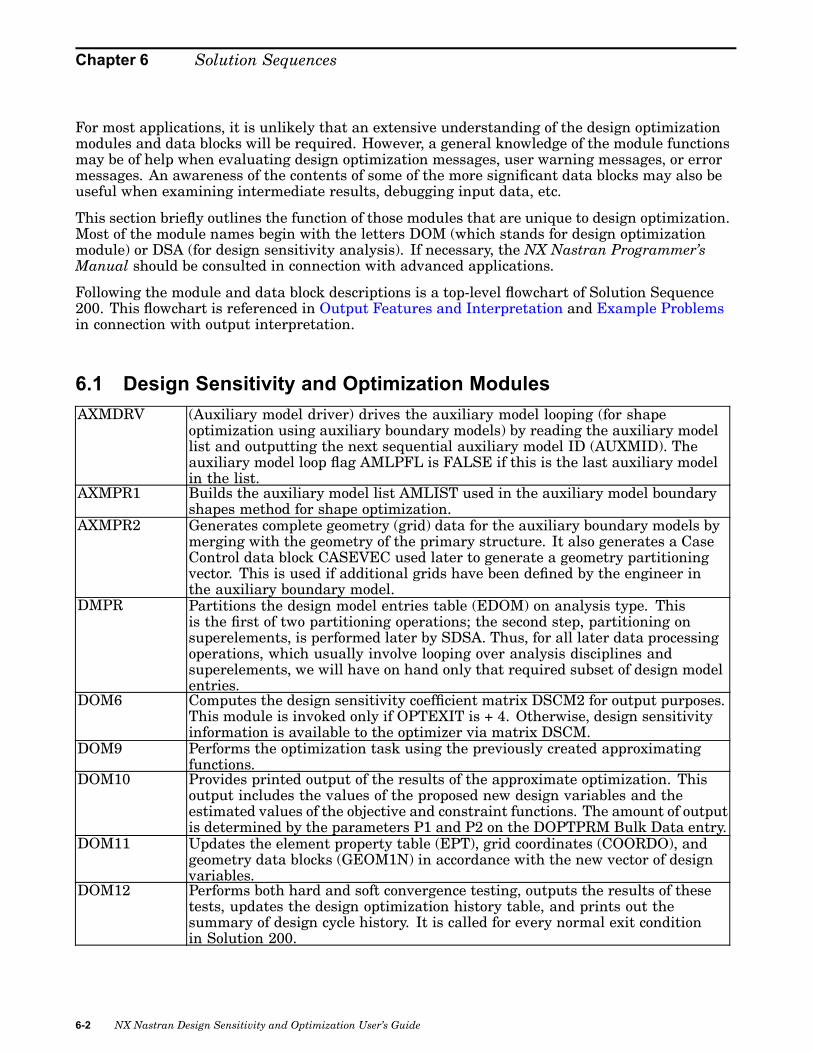
Chapter 6 Solution Sequences
For most applications, it is unlikely that an extensive understanding of the design optimizationmodules and data blocks will be required. However, a general knowledge of the module functionsmay be of help when evaluating design optimization messages, user warning messages, or errormessages. An awareness of the contents of some of the more significant data blocks may also beuseful when examining intermediate results, debugging input data, etc.
This section briefly outlines the function of those modules that are unique to design optimization.Most of the module names begin with the letters DOM (which stands for design optimizationmodule) or DSA (for design sensitivity analysis). If necessary, the NX Nastran Programmer’sManual should be consulted in connection with advanced applications.
Following the module and data block descriptions is a top-level flowchart of Solution Sequence200. This flowchart is referenced in Output Features and Interpretation and Example Problemsin connection with output interpretation.
6.1 Design Sensitivity and Optimization ModulesAXMDRV (Auxiliary model driver) drives the auxiliary model looping (for shape
optimization using auxiliary boundary models) by reading the auxiliary modellist and outputting the next sequential auxiliary model ID (AUXMID). Theauxiliary model loop flag AMLPFL is FALSE if this is the last auxiliary modelin the list.
AXMPR1 Builds the auxiliary model list AMLIST used in the auxiliary model boundaryshapes method for shape optimization.
AXMPR2 Generates complete geometry (grid) data for the auxiliary boundary models bymerging with the geometry of the primary structure. It also generates a CaseControl data block CASEVEC used later to generate a geometry partitioningvector. This is used if additional grids have been defined by the engineer inthe auxiliary boundary model.
DMPR Partitions the design model entries table (EDOM) on analysis type. Thisis the first of two partitioning operations; the second step, partitioning onsuperelements, is performed later by SDSA. Thus, for all later data processingoperations, which usually involve looping over analysis disciplines andsuperelements, we will have on hand only that required subset of design modelentries.
DOM6 Computes the design sensitivity coefficient matrix DSCM2 for output purposes.This module is invoked only if OPTEXIT is + 4. Otherwise, design sensitivityinformation is available to the optimizer via matrix DSCM.
DOM9 Performs the optimization task using the previously created approximatingfunctions.
DOM10 Provides printed output of the results of the approximate optimization. Thisoutput includes the values of the proposed new design variables and theestimated values of the objective and constraint functions. The amount of outputis determined by the parameters P1 and P2 on the DOPTPRM Bulk Data entry.
DOM11 Updates the element property table (EPT), grid coordinates (COORDO), andgeometry data blocks (GEOM1N) in accordance with the new vector of designvariables.
DOM12 Performs both hard and soft convergence testing, outputs the results of thesetests, updates the design optimization history table, and prints out thesummary of design cycle history. It is called for every normal exit conditionin Solution 200.
6-2 NX Nastran Design Sensitivity and Optimization User’s Guide
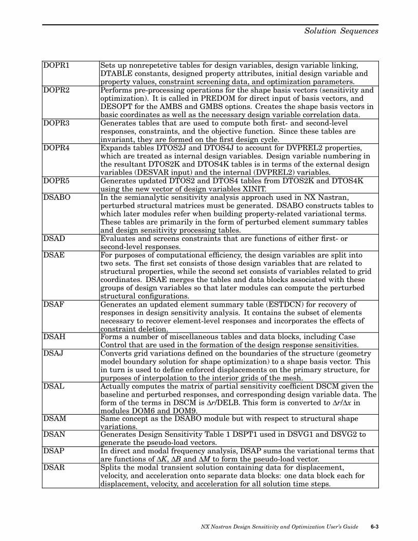
Solution Sequences
DOPR1 Sets up nonrepetetive tables for design variables, design variable linking,DTABLE constants, designed property attributes, initial design variable andproperty values, constraint screening data, and optimization parameters.
DOPR2 Performs pre-processing operations for the shape basis vectors (sensitivity andoptimization). It is called in PREDOM for direct input of basis vectors, andDESOPT for the AMBS and GMBS options. Creates the shape basis vectors inbasic coordinates as well as the necessary design variable correlation data.
DOPR3 Generates tables that are used to compute both first- and second-levelresponses, constraints, and the objective function. Since these tables areinvariant, they are formed on the first design cycle.
DOPR4 Expands tables DTOS2J and DTOS4J to account for DVPREL2 properties,which are treated as internal design variables. Design variable numbering inthe resultant DTOS2K and DTOS4K tables is in terms of the external designvariables (DESVAR input) and the internal (DVPREL2) variables.
DOPR5 Generates updated DTOS2 and DTOS4 tables from DTOS2K and DTOS4Kusing the new vector of design variables XINIT.
DSABO In the semianalytic sensitivity analysis approach used in NX Nastran,perturbed structural matrices must be generated. DSABO constructs tables towhich later modules refer when building property-related variational terms.These tables are primarily in the form of perturbed element summary tablesand design sensitivity processing tables.
DSAD Evaluates and screens constraints that are functions of either first- orsecond-level responses.
DSAE For purposes of computational efficiency, the design variables are split intotwo sets. The first set consists of those design variables that are related tostructural properties, while the second set consists of variables related to gridcoordinates. DSAE merges the tables and data blocks associated with thesegroups of design variables so that later modules can compute the perturbedstructural configurations.
DSAF Generates an updated element summary table (ESTDCN) for recovery ofresponses in design sensitivity analysis. It contains the subset of elementsnecessary to recover element-level responses and incorporates the effects ofconstraint deletion.
DSAH Forms a number of miscellaneous tables and data blocks, including CaseControl that are used in the formation of the design response sensitivities.
DSAJ Converts grid variations defined on the boundaries of the structure (geometrymodel boundary solution for shape optimization) to a shape basis vector. Thisin turn is used to define enforced displacements on the primary structure, forpurposes of interpolation to the interior grids of the mesh.
DSAL Actually computes the matrix of partial sensitivity coefficient DSCM given thebaseline and perturbed responses, and corresponding design variable data. Theform of the terms in DSCM is Δr/DELB. This form is converted to Δr/Δx inmodules DOM6 and DOM9.
DSAM Same concept as the DSABO module but with respect to structural shapevariations.
DSAN Generates Design Sensitivity Table 1 DSPT1 used in DSVG1 and DSVG2 togenerate the pseudo-load vectors.
DSAP In direct and modal frequency analysis, DSAP sums the variational terms thatare functions of ΔK, ΔB and ΔM to form the pseudo-load vector.
DSAR Splits the modal transient solution containing data for displacement,velocity, and acceleration onto separate data blocks: one data block each fordisplacement, velocity, and acceleration for all solution time steps.
NX Nastran Design Sensitivity and Optimization User’s Guide 6-3

Chapter 6 Solution Sequences
DSAW Computes the delta weight and/or volume according to the changes in thedesign variables in connection with the semi-analytic sensitivity analysis.
DSPRM Outputs parameters used for DMAP flow control. Depending on the typesof retained responses listed in data block DRSTBL, parameters are outputto indicate whether or not response sensitivities are to be recovered for aparticular superelement.
DSTAP2 Generates a correlation table describing the design response column order forthe DSCM/DSCM2 matrices.
DSVG1 (Design Sensitivity Vector Generator 1) computes terms in the pseudo-loadvectors for sensitivity analysis that depend on ΔK, ΔB, and ΔM.
DSVG2 Design Sensitivity Vector Generator 2. This module computes the thermal loadcontribution to the pseudo-load vector.
DSVG4 Design Sensitivity Vector Generator 4. Forms u + Δu finite difference change indisplacements for design variables that affect mass and/or stiffness terms.
MDCASE Partitions the original input case control onto individual Case Control recordsbased on analysis type. It also outputs parameters that are used at the DMAPlevel to direct analysis for the various disciplines.
SDSA Partitions the design model entries table (EDOM) on superelement. The result,EDOMS, is an analysis discipline and superelement partition of the originalEDOM. See also the DMPR module description.
SDSB Builds the superelement design sensitivity processing data block DSLIST thatis used to direct the pseudo-load and response sensitivity superement loops. Itsstructure is similar to SLIST, used in superelement analysis.
SDSC Prints the DSCMR correlation table that identifies the column-responsecorrelation in the design sensitivity coefficient matrix DSCM2.
SHPCAS Generates a new Case Control data block to drive solutions for basis vectorsin shape optimization. The initial shape data is supplied as enforceddisplacements on the boundary of the structure and then interpolated to theinterior grids via a static solution of the primary structure. SHPCAS generatesthe Case Control data block CASENEW, which is used in connection with thissolution. It also generates a partitioning vector CVEC to extract the appropriatesolution vectors from the analysis results.
WEIGHT Computes the structural weight or volume for use in design optimization.Weight (or mass) is only computed for those elements that have volume. Theeffect of elements such as CONMs are thus neglected.
6.2 Selected Data BlocksThe data blocks listed in this section are of particular interest in design sensitivity andoptimization. Although just a subset, the data blocks listed here have been chosen based on theirusefulness in custom DMAPing, results processing, etc.
Should the need arise, the brief descriptions in this section may be a useful aid when trying tonavigate through various sections of the DMAP. The module that creates each data block is notedat the end of each description. Full descriptions of these data blocks’ content and format can befound in the NX Nastran Programmer’s Manual.
Design Model DefinitionCVALO Updated approximate constraint values output from the optimizer. (DOM9)
6-4 NX Nastran Design Sensitivity and Optimization User’s Guide

Solution Sequences
DESTAB Table containing design variable attributes. (DOPR1)
DTOS2 Table, built from DTOS2K, containing current values of designed properties. Thisis updated at the beginning of every design cycle. (DOPR5)
DTOS2J Table identifying properties referenced in the design model, both DVPREL1 andDVPREL2. This is built directly from the design model data. (DOPR1)
DTOS2K Same as DTOS2J, but rearranged on internal design variable order. (DOPR4)
EDOM Table containing design model data. (IFP)
EDOMS Analysis discipline- and superelement-partitioned EDOM. (SDSA)
EPTN Updated element property tables, based on optimization results. (DOM11)
GEOM1N Updated grid (geometry) records, based on the optimization results. (DOM11)
PROPO Vector of properties output from the optimizer. (DOM9)
R1VALO First-level responses output from the optimizer. These are based on theapproximate model. (DOM9)
R2VALO Second-level responses output from the optimizer. These are based on theapproximate model. (DOM9)
TABDEQ Table of unique design variable IDs. (DOPR4)
XINIT Vector of initial design variable values, updated at the start of each design cycle.(DOPR1 initialization, EQUIVX after DOM9 on subsequent cycles.)
XO Vector of design variables output from the optimizer. This becomes XINIT forthe next design cycle. (DOM9)
Shape OptimizationAMLIST List of auxiliary models that is used to drive auxiliary model loops for shape
optimization. (AXMPR1)
NX Nastran Design Sensitivity and Optimization User’s Guide 6-5

Chapter 6 Solution Sequences
BASVEC Basis vectors for shape optimization. This form is G-set size and is in basiccoordinates. It is used in the AMBS, GMBS, and external input of basis vectorsmethods. (VECPLOT for AMBS and GMBS, SMPYAD for External Input.)
COORDO Old set of coordinate values, for designed grids only. It is constant over all designcycles for the external input of basis vectors method and is updated on every designcycle for AMBS and GMBS. (DOPR2)
COORDN New set of coordinate values for designed grids only. Its purpose is to provide theDNODE input data for the DRESP2 Bulk Data entries. (DOM11)
CVEC Partitioning vector used to strip out the shape basis vector solutions for the AMBSand GMBS methods. (SHPCAS)
DELBSH A vector defining the finite difference moves to be used in shape sensitivity. It iscomputed based on shape basis vector energy norms. (ADD5)
DESGID List of designed coordinates, and identification data. (DOPR2)
DTOS4 Table containing designed grid perturbations. Its form is the same as DTOS4K andis used to define element-level variations for shape sensitivity analysis. (DOPR5)
DTOS4J Table of shape basis vector data. It is in external (user-defined) design variableID order. (DOPR2)
DTOS4K Differs from DTOS4J only in that it is sorted on internal design variable ID.(DOPR4)
DVIDS Design variables related to shape changes. (DSAJ)
DESVCP Basis vectors for shape optimization, G-set size, expressed in the global coordinatesystem. DESVECP contains one column for each independent design variable. It isgenerated primarily for energy norm based step size determination. (DOPR2)
SHPVEC Basis vectors for shape optimization, although it contains only designed grids. Itis expressed in global coordinates with one column for each independent designvariable. (DOPR2)
UGBSHP G-set size basis vectors in the global coordinate system. It contains information forall grids in the model. (PARTN)
6-6 NX Nastran Design Sensitivity and Optimization User’s Guide

Solution Sequences
Constraint Evaluation and ScreeningCASEDS Case Control for the recovery of design responses. (DOPR3)
DRSTBL Table providing the number of retained responses for each subcase for each of theresponse types. (DSAD)
R1VAL Vector of type 1 response values. (DSAD)
R2VAL Vector of type 2 response values. (DSAD)
R1VALR Vector of retained type 1 response values. (DSAD)
R2VALR Vector of retained type 2 response values. (DSAD)
CVAL Vector of constraint values. (DSAD)
CVALR Vector of retained constraint values. (DSAD)
Design Sensitivity AnalysisDELWS Delta weight. (DSAW)
DELVS Delta volume. (DSAW)
DSCM Design sensitivity coefficient matrix, form 1. Each term is Δr/DELB. (DSAL)
DSCM2 Design sensitivity coefficient matrix, form 2 (generated for output purposes only).Each term is Δr/Δx. (DOM6)
DSCMCOL Correlation table for DSCM. (DSTAP2, SDSC)
ESTDVP Perturbed element summary table used to compute property sensitivities.(DSABO)
ESTDVS Perturbed element summary table used to compute shape sensitivities. (DSAM)
EGK Pseudo-load contributions from changes in K. (DSVG1)
EGM Pseudo-load contributions from changes in M. (DSVG1)
NX Nastran Design Sensitivity and Optimization User’s Guide 6-7

Chapter 6 Solution Sequences
EGB Pseudo-load contributions from changes in B. (DSVG1)
Design Optimization HistoryHIS Design optimization history table. (DOM12?APPEND?EQUIVX)
HISADD Additions to the design optimization history table due to the current design cycle.(DOM12)
NEWPRM Update of design optimization parameters (due to the automatic reduction of movelimits). (DOM12)
GeneralDSLIST Superelement processing list for design optimization-similar to an SLIST for
superelement analysis. (SDSB)
DTB Constants from the DTABLE Bulk Data entry. (DOPR1)
OPTPRM Optimization parameters. (DOPR1)
6.3 Solution 200 Program FlowDesign sensitivity analysis and optimization both are only available in Solution Sequence 200.The following flowchart describes the organization of Solution 200 or main subDMAP DESOPTas well as listing some of the more significant modules and subDMAPs invoked.
Each of the boxes in this high-level flowchart describes a major program phase as well as thedesign sensitivity and/or optimization modules used to accomplish that particular task. Thesemodule names are included inside each of the boxes. If program flow is directed to a particularsubDMAP, each name is listed alongside each of the boxes.
Finite element analysis and sensitivity analysis are the most computationally-intensivephases. These CPU-intensive phases have been highlighted in the flowchart.
The circled numbers 1 through 6 appearing in the flowchart indicate the locations of the sixuser-defined exit points. Any one of these exits can be taken by setting the parameter OPTEXITto an integer value from 1 through 6.
An OPTEXIT value of 7 provides sensitivity coefficient output upon normal program termination(the sensitivities are printed to the .F06 output file.) Normal program termination includes bothhard and soft convergence, and maximum number of design cycles. Sensitivities for the finaldesign may be particularly useful depending on your postprocessing requirements. Be awarehowever, that some additional costs will be incurred for the hard convergence exit condition sincethe sensitivities must be recomputed for the last design cycle.
6-8 NX Nastran Design Sensitivity and Optimization User’s Guide

Solution Sequences
NX Nastran Design Sensitivity and Optimization User’s Guide 6-9

Chapter 6 Solution Sequences
6-10 NX Nastran Design Sensitivity and Optimization User’s Guide

Solution Sequences
NX Nastran Design Sensitivity and Optimization User’s Guide 6-11

Chapter 6 Solution Sequences
6-12 NX Nastran Design Sensitivity and Optimization User’s Guide

Chapter
7 Example Problems
• Three-Bar Truss
• Vibration of a Cantilever Beam (Turner’s Problem)
• Cantilevered Plate
• Stiffened Plate
• Shape Optimization of a Culvert
• Analytic Boundary Shapes
• Dynamic Response Optimization
• Twenty-Five Bar Truss, Superelement Optimization
• Design Optimization with Composite Materials
• Acoustic Optimization
• Restarts in Design Optimization
NX Nastran Design Sensitivity and Optimization User’s Guide 7-1

Chapter 7 Example Problems
This chapter includes a wide range of examples intended to highlight and illustrate the DesignSensitivity and Optimization features of the software. Though by no means exhaustive, theseeleven examples cover most major features including both Property and Shape Optimization,Dynamic Response Optimization, Superelements, Composites, Acoustic Responses, and Restarts.Aeroelastic Optimization examples are presented in the NX Nastran Aeroelastic Analysis User’sGuide.
The results in this chapter have been obtained running on an IBM RISC System/6000workstation. Although your results may differ slightly, running these examples on your ownmachine is a good way to familiarize yourself with some of the software’s capabilities. All of thesedecks are available in the NX Nastran Test Problem Library, delivered with your system. If youare unable to find these files, you should contact your System Administrator for assistance.
Another good way to learn is by modifying these decks. You might try adding Shape variables toa Property Optimization example, adding analysis disciplines, modifying the constraints, and soon. Most of these decks are relatively small, and should not incur any great CPU-related costs.In any event, the time spent learning with simple examples can more than pay for itself whenfaced with larger, more complex, problems.
Examples in this chapter include:
Three-Bar Truss TPL problem D200X1.DATThis is a classic getting started example. It examines weightminimization of a structure subject to stress and displacementconstraints from multiple statics subcases. Design Variables arelinearly related to rod cross-sectional areas. It introduces explicitdesign variable linking.
Vibration of a CantileverBeam (Turner’s Problem)
TPL problem D200X6.DAT
Examines weight minimization of a structure subject to afree-vibration frequency constraint. Design variables are linearlyrelated to rod areas and shell thickness. Discusses interpretation ofweight objective function if concentrated masses are used.
Cantilevered Plate TPL problem D200X5.DATIllustrates reduced-basis formulation using explicit design variablelinking (DLINK). Weight minimization of a statically loaded platewith constraints on principal and von Mises stresses as well as griddisplacements.
Stiffened Plate TPL problem D200X7.DATIllustrates effective grouping of elements by property type for designmodeling purposes and use of the DVPREL2 entry for user-definedproperty relations. Weight minimization subject to constrains onstatic stresses and displacements. Design variables are related toplate thicknesses and bar cross-sectional properties.
Shape Optimization of aCulvert
TPL problems D200CSX.DAT, D200CS.DAT
7-2 NX Nastran Design Sensitivity and Optimization User’s Guide
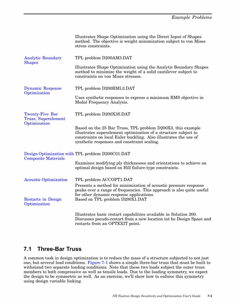
Example Problems
Illustrates Shape Optimization using the Direct Input of Shapesmethod. The objective is weight minimization subject to von Misesstress constraints.
Analytic BoundaryShapes
TPL problem D200AM3.DAT
Illustrates Shape Optimization using the Analytic Boundary Shapesmethod to minimize the weight of a solid cantilever subject toconstraints on von Mises stresses.
Dynamic ResponseOptimization
TPL problem D200RML3.DAT
Uses synthetic responses to express a minimum RMS objective inModal Frequency Analysis.
Twenty-Five BarTruss, SuperelementOptimization
TPL problem D200X3S.DAT
Based on the 25 Bar Truss, TPL problem D200X3, this exampleillustrates superelement optimization of a structure subject toconstraints on local Euler buckling. Also illustrates the use ofsynthetic responses and constraint scaling.
Design Optimization withComposite Materials
TPL problem D200C01.DAT
Examines modifying ply thicknesses and orientations to achieve anoptimal design based on Hill failure-type constraints.
Acoustic Optimization TPL problem ACCOPT1.DATPresents a method for minimization of acoustic pressure responsepeaks over a range of frequencies. This approach is also quite usefulfor other dynamic response applications.
Restarts in DesignOptimization
Based on TPL problem D200X1.DAT
Illustrates basic restart capabilities available in Solution 200.Discusses pseudo-restart from a new location int he Design Space andrestarts from an OPTEXIT point.
7.1 Three-Bar TrussA common task in design optimization is to reduce the mass of a structure subjected to not justone, but several load conditions. Figure 7-1 shows a simple three-bar truss that must be built towithstand two separate loading conditions. Note that these two loads subject the outer trussmembers to both compressive as well as tensile loads. Due to the loading symmetry, we expectthe design to be symmetric as well. As an exercise, we’ll show how to enforce this symmetryusing design variable linking.
NX Nastran Design Sensitivity and Optimization User’s Guide 7-3

Chapter 7 Example Problems
An important, but often overlooked consideration is that the optimization capability in NXNastran is multidisciplinary. That is, the final optimal design is the result of a simultaneousconsideration of all analysis disciplines across all subcases. In this case, the optimal three-bartruss design will satisfy the load requirements for both statics subcases, which is to be expected.(If, for example, a normal modes subcase were to be added, the resultant design would have tonot only satisfy the static strength requirements, but also constraints on eigenvalues. As anexercise you may wish to try adding an eigenvalue constraint.
Figure 7-1. Three-Bar Truss.
Analysis Model Description
Three rod (pin-jointed) structure in the x-y planeSymmetric structural configuration with respect to the y-axisTwo distinct 20,000 lb load conditionsMaterial: E = 1.0E7 psi
Weight density = 0.1 lbs/in3
Design Model Description
Objective: Minimization of structural weightDesign variable: Cross-sectional areas A1, A2, and A3
Design variable linking such that A3 = A1Constraints: Allowable stress: Tensile 20,000 psi
Compressive = -15,000 psi
7-4 NX Nastran Design Sensitivity and Optimization User’s Guide

Example Problems
The input data for this problem is given in Listing 7-1. Grid, element, and load data are assignedbased on the data supplied in the figure. The two separate static load cases are defined inSolution 200 Case Control using the parameter ANALYSIS = STATICS.
Turning to the design model description, we see three design variables are used, one each tocontrol the individual rod element cross-sectional areas. The set of DESVAR, DVPREL1 entriesdefine the relations:
Equation 7-1.
Note that the initial design variable values are equal to the initial rod cross-sectional areas.With the multiplying coefficients of 1.0 on the DVPREL1 entries, the design model and the initialanalysis model properties agree. Thus, no design model override takes place.
Since the model’s geometry and loading are both symmetric, we expect the optimizer to yielda symmetric final design with A1 = A3. In a more complex structure, we may want to enforcesome type of continuity ourselves, perhaps to address ease-of-manufacture concerns. This can bedone using the DLINK entry to explicitly link design variables together. Although not strictlynecessary, DLINK 1 is used to define the relation
Equation 7-2.
The value of X3 now depends on X1. The optimizer now only needs to consider two independentdesign variables X1 and X 2 instead of three. This not only simplifies the problem, but also reducesthe cost of the sensitivity analysis. This cost savings can be significant in a larger problem.
An alternate method of linking would have been placing rod elements 11 and 13 in the sameproperty group. The DLINK entry would then be unnecessary since a single design variablecould control the areas of all elements of the group. You may want to try this formulation yourselfto see that the results are indeed identical.
DRESP1 entries define the design responses: displacement and stress responses that are to beconstrained and the weight response that is to be used as the objective. Note that the objectiveand constraints are called out in Case Control. The DESOBJ command points to the weightresponse defined on DRESP1 20, while the DESSUB command identifies DCONSTR set 21. Sincethis appears above the subcase level, the constraint bounds will be applied to both subcases.
A DOPTPRM entry is used to override some of the default optimization parameters. DESMAX,or the maximum number of design cycles to be performed, has been increased from the defaultof 5 to 10. (If convergence is indicated, fewer than 10 cycles may be performed.) DELP hasalso been increased from its default of 0.2 to 0.5. This allows any analysis model parameter toundergo changes of up to 50% on each design cycle. This provides move limits on the approximatemodel. And finally, IPRINT, P1, and P2 have all been increased from their defaults to allowmore diagnostic output.
Turning to the results of the optimization, we see from the hard convergence decision logicoutput that the problem converges to a feasible design since all constraints are satisfied at theoptimum. However, note that the properties and design variables have still changed appreciablyfrom their values on the previous design cycle. This suggests that we may have some flexibilityin choosing final dimensions for our design without greatly affecting the overall weight.
NX Nastran Design Sensitivity and Optimization User’s Guide 7-5

Chapter 7 Example Problems
The summary of design cycle history and the design variable history tables both indicate thatconvergence was achieved in five iterations. A total of six finite element analyses were performed,one for the initial analysis and one in connection with each of the design cycles. Also listed in thesummary of design cycle history is the fractional error of approximation in the objective function,which compares the approximate objective function on exit from the optimizer with the truevalue computed from the subsequent finite element analysis. This is an indication of the qualityof the objective function approximation. Since the weight is linear in the design variables (W =L1X1 + L2X2 + L3L3), we expect the linearized weight objective to be an exact approximation; thisindeed is seen to be the case, except for a small amount of numerical "noise." Caution should beused when interpreting the data appearing in the fractional error of approximation column.
One might be tempted to use the fractional error of approximation information as justificationfor increasing the move limits (DELP and DELX on the DOPTPRM entry, and/or DELXV on theDESVAR entry) in order to achieve convergence earlier. This might not yield the expected results.In this case, the linear objective function was approximated linearly, which is exact. However,the stress constraints in this problem are proportional to the inverse of the cross-sectionalareas, and are thus nonlinear in the design variables. Too large of a move limit could lead toincreased approximation errors as was illustrated in Chapter 3. Here, the mixed method ofapproximation was used, which we know to be pretty good at approximating sizing-type stressconstraints. Thus, increasing move limits to 50% is reasonable, as it will probably save us thecost of a few additional finite element analyses. A recommendation would be to stick with thedefaults, unless something is known about the problem beforehand that would indicate enhancedefficiency by changing them.
***** NORMAL CONVERGENCE CRITERIA SATISFIED ***** (HARD CONVERGENCE DECISION LOGIC)**************************************************************************************
CONVERGENCE ACHIEVED BASED ON THE FOLLOWING CRITERIA(HARD CONVERGENCE DECISION LOGIC)
RELATIVE CHANGE IN OBJECTIVE 2.7611E-03 MUST BE LESS THAN 1.0000E-03OR ABSOLUTE CHANGE IN OBJECTIVE 7.4799E-03 MUST BE LESS THAN 1.0000E-02
--- AND ---MAXIMUM CONSTRAINT VALUE -9.2676E-05 MUST BE LESS THAN 5.0000E-03
(CONVERGENCE TO A FEASIBLE DESIGN)--- OR ---
MAXIMUM OF RELATIVE PROP. CHANGES 1.5165E-01 MUST BE LESS THAN 1.0000E-03AND MAXIMUM OF RELATIVE D.V. CHANGES 1.5165E-01 MUST BE LESS THAN 1.0000E-03
(CONVERGENCE TO A BEST COMPROMISE INFEASIBLE DESIGN)**************************************************************************************
***************************************************************S U M M A R Y O F D E S I G N C Y C L E H I S T O R Y***************************************************************
(HARD CONVERGENCE ACHIEVED)NUMBER OF FINITE ELEMENT ANALYSES COMPLETED 6NUMBER OF OPTIMIZATIONS W.R.T. APPROXIMATE MODELS 5
OBJECTIVE AND MAXIMUM CONSTRAINT HISTORY---------------------------------------------------------------------------------------------------------------
OBJECTIVE FROM OBJECTIVE FROM FRACTIONAL ERROR MAXIMUM VALUE ROW OFCYCLE APPROXIMATE EXACT OF OF MAXIMUMNUMBER OPTIMIZATION ANALYSIS APPROXIMATION CONSTRAINT CONSTRAINT
---------------------------------------------------------------------------------------------------------------INITIAL 4.828427E+00 -3.234952E-01 2
1 3.007858E+00 3.008487E+00 -2.093749E-04 -3.737109E-03 22 2.820099E+00 2.819910E+00 6.696224E-05 -1.902266E-02 33 2.735039E+00 2.735147E+00 -3.957449E-05 -7.482129E-03 34 2.709055E+00 2.709030E+00 9.152918E-06 -2.097656E-04 35 2.701577E+00 2.701550E+00 9.884281E-06 -9.267578E-05 2
---------------------------------------------------------------------------------------------------------------
7-6 NX Nastran Design Sensitivity and Optimization User’s Guide
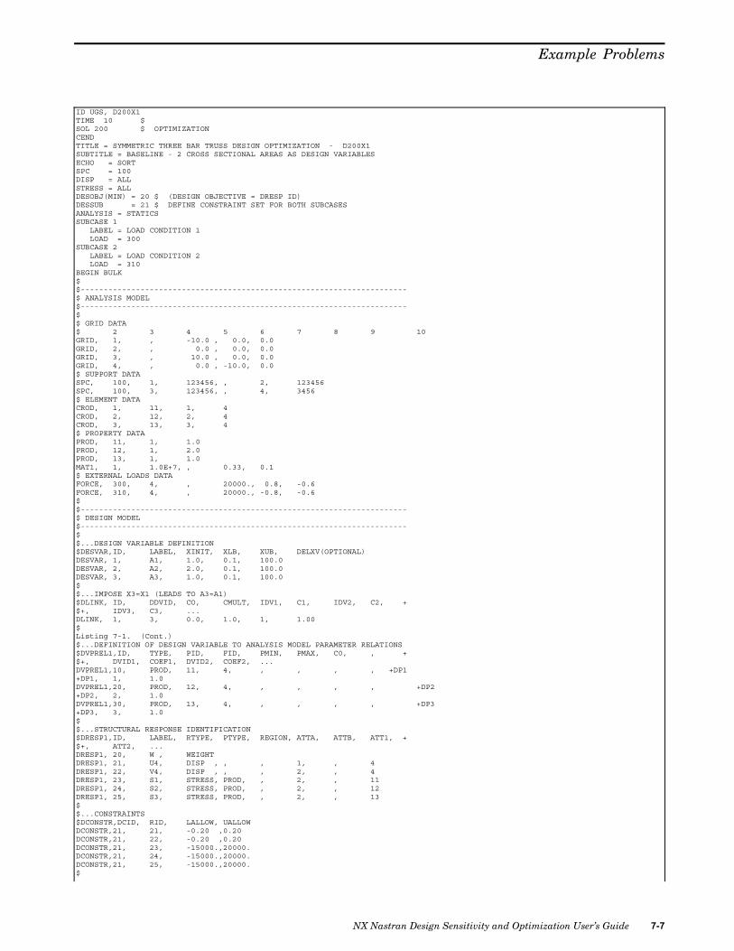
Example Problems
ID UGS, D200X1TIME 10 $SOL 200 $ OPTIMIZATIONCENDTITLE = SYMMETRIC THREE BAR TRUSS DESIGN OPTIMIZATION - D200X1SUBTITLE = BASELINE - 2 CROSS SECTIONAL AREAS AS DESIGN VARIABLESECHO = SORTSPC = 100DISP = ALLSTRESS = ALLDESOBJ(MIN) = 20 $ (DESIGN OBJECTIVE = DRESP ID)DESSUB = 21 $ DEFINE CONSTRAINT SET FOR BOTH SUBCASESANALYSIS = STATICSSUBCASE 1
LABEL = LOAD CONDITION 1LOAD = 300
SUBCASE 2LABEL = LOAD CONDITION 2LOAD = 310
BEGIN BULK$$-----------------------------------------------------------------------$ ANALYSIS MODEL$-----------------------------------------------------------------------$$ GRID DATA$ 2 3 4 5 6 7 8 9 10GRID, 1, , -10.0 , 0.0, 0.0GRID, 2, , 0.0 , 0.0, 0.0GRID, 3, , 10.0 , 0.0, 0.0GRID, 4, , 0.0 , -10.0, 0.0$ SUPPORT DATASPC, 100, 1, 123456, , 2, 123456SPC, 100, 3, 123456, , 4, 3456$ ELEMENT DATACROD, 1, 11, 1, 4CROD, 2, 12, 2, 4CROD, 3, 13, 3, 4$ PROPERTY DATAPROD, 11, 1, 1.0PROD, 12, 1, 2.0PROD, 13, 1, 1.0MAT1, 1, 1.0E+7, , 0.33, 0.1$ EXTERNAL LOADS DATAFORCE, 300, 4, , 20000., 0.8, -0.6FORCE, 310, 4, , 20000., -0.8, -0.6$$-----------------------------------------------------------------------$ DESIGN MODEL$-----------------------------------------------------------------------$$...DESIGN VARIABLE DEFINITION$DESVAR,ID, LABEL, XINIT, XLB, XUB, DELXV(OPTIONAL)DESVAR, 1, A1, 1.0, 0.1, 100.0DESVAR, 2, A2, 2.0, 0.1, 100.0DESVAR, 3, A3, 1.0, 0.1, 100.0$$...IMPOSE X3=X1 (LEADS TO A3=A1)$DLINK, ID, DDVID, CO, CMULT, IDV1, C1, IDV2, C2, +$+, IDV3, C3, ...DLINK, 1, 3, 0.0, 1.0, 1, 1.00$Listing 7-1. (Cont.)$...DEFINITION OF DESIGN VARIABLE TO ANALYSIS MODEL PARAMETER RELATIONS$DVPREL1,ID, TYPE, PID, FID, PMIN, PMAX, C0, , +$+, DVID1, COEF1, DVID2, COEF2, ...DVPREL1,10, PROD, 11, 4, , , , , +DP1+DP1, 1, 1.0DVPREL1,20, PROD, 12, 4, , , , , +DP2+DP2, 2, 1.0DVPREL1,30, PROD, 13, 4, , , , , +DP3+DP3, 3, 1.0$$...STRUCTURAL RESPONSE IDENTIFICATION$DRESP1,ID, LABEL, RTYPE, PTYPE, REGION, ATTA, ATTB, ATT1, +$+, ATT2, ...DRESP1, 20, W , WEIGHTDRESP1, 21, U4, DISP , , , 1, , 4DRESP1, 22, V4, DISP , , , 2, , 4DRESP1, 23, S1, STRESS, PROD, , 2, , 11DRESP1, 24, S2, STRESS, PROD, , 2, , 12DRESP1, 25, S3, STRESS, PROD, , 2, , 13$$...CONSTRAINTS$DCONSTR,DCID, RID, LALLOW, UALLOWDCONSTR,21, 21, -0.20 ,0.20DCONSTR,21, 22, -0.20 ,0.20DCONSTR,21, 23, -15000.,20000.DCONSTR,21, 24, -15000.,20000.DCONSTR,21, 25, -15000.,20000.$
NX Nastran Design Sensitivity and Optimization User’s Guide 7-7

Chapter 7 Example Problems
$...OPTIMIZATION CONTROL:$DOPTPRM,IPRINT, 5, DESMAX, 10, DELP, 0.5, P1, 1, ++, P2, 15$$.......2.......3.......4.......5.......6.......7.......8.......9......0ENDDATA
Listing 7-1.
7.2 Vibration of a Cantilever Beam (Turner’s Problem)This problem was originally published by M.J. Turner ("Design of Minimum Mass Structureswith Specified Natural Frequencies," AIAA Journal Vol. 5, No. 3, March 1967). The problem isto design a minimum weight structure while constraining the fundamental bending frequencyat or above 20 Hz. The beam is symmetric and made up of a shear web having top and bottomcaps that are modeled with rod elements. Turner’s original design model consisted of piecewiselinear bar cross-sectional areas and web thicknesses; however, we will just approximate this asa step function model with uniform cross-sectional rod elements and uniform thickness shearelements within each of three bays.
Figure 7-2. Cantilever Beam Vibration Model.
Analysis Model DescriptionWeb is modeled by QUAD4 elementsCaps are modeled by ROD elementsMaterial: E = 1.03E7 psi
Poisson ratio = 0.3Weight density = 0.1 lbs/in3
Non-structuralmass:
Lumped masses at top and bottom nodes, 15 lbs. each
Design Model DescriptionObjective: Minimization of structural weight
7-8 NX Nastran Design Sensitivity and Optimization User’s Guide

Example Problems
Design variables: Cross-sectional areas of bar elements (symmetry imposed on thetop and bottom elements)
Constraints: Fundamental bending frequency at or above 20 Hz
Normal modes analysis is requested in Solution 200 by setting the Case Control parameterANALYSIS = MODES. In order to determine a minimum weight design subject to a lower-boundconstraint on fundamental frequency, the thicknesses of the three shear panels and the sixrod cross-sectional areas are allowed to vary. These variations are described using six designvariables; three for the web thicknesses and three for the rod cross-sectional areas (symmetry isimposed on the upper and lower ROD element areas.) See Listing 7-2 for details.
The lower-bound constraint on the first mode is 20 Hz. Note that the DCONSTR entry places
bounds on λ = (2πf )2 , or . The upper bound will not drive the design, so it is just set toan arbitrarily large value of 2.0E5.
It should be noted that the weight (or, more appropriately, mass) objective function is computedin NX Nastran based on a volume • calculation. Thus, elements that have no volume are notincluded in the weight response calculation. Here, the mass contribution of the concentratedmasses is ignored, as can be verified from the summary of design cycle history. In general,although concentrated and distributed masses are not included in the design model responses,they are accounted for, as expected, in the analysis.
Turning to the optimization results, we note that hard convergence has been achieved after fivedesign cycles, requiring a total of six finite element analyses. We note that a feasible designhas been achieved as the maximum constraint value is less than the allowable maximum.Again, the final "weight" objective is that due to the plate and rod elements only, excludingthe concentrated masses.
***** NORMAL CONVERGENCE CRITERIA SATISFIED ***** (HARD CONVERGENCE DECISION LOGIC)**************************************************************************************
CONVERGENCE ACHIEVED BASED ON THE FOLLOWING CRITERIA(HARD CONVERGENCE DECISION LOGIC)
RELATIVE CHANGE IN OBJECTIVE 2.0467E-04 MUST BE LESS THAN 1.0000E-03OR ABSOLUTE CHANGE IN OBJECTIVE 1.4267E-03 MUST BE LESS THAN 1.0000E-02
--- AND ---MAXIMUM CONSTRAINT VALUE 1.7216E-03 MUST BE LESS THAN 5.0000E-03
(CONVERGENCE TO A FEASIBLE DESIGN)--- OR ---
MAXIMUM OF RELATIVE PROP. CHANGES 2.3337E-02 MUST BE LESS THAN 1.0000E-03AND MAXIMUM OF RELATIVE D.V. CHANGES 2.3337E-02 MUST BE LESS THAN 1.0000E-03
(CONVERGENCE TO A BEST COMPROMISE INFEASIBLE DESIGN)**************************************************************************************
***************************************************************S U M M A R Y O F D E S I G N C Y C L E H I S T O R Y***************************************************************
(HARD CONVERGENCE ACHIEVED)NUMBER OF FINITE ELEMENT ANALYSES COMPLETED 6NUMBER OF OPTIMIZATIONS W.R.T. APPROXIMATE MODELS 5
OBJECTIVE AND MAXIMUM CONSTRAINT HISTORY---------------------------------------------------------------------------------------------------------------
OBJECTIVE FROM OBJECTIVE FROM FRACTIONAL ERROR MAXIMUM VALUE ROW OFCYCLE APPROXIMATE EXACT OF OF MAXIMUMNUMBER OPTIMIZATION ANALYSIS APPROXIMATION CONSTRAINT CONSTRAINT
---------------------------------------------------------------------------------------------------------------INITIAL 1.920000E+01 0.000000E+00 0
1 9.599560E+00 9.599990E+00 -4.480287E-05 9.583312E-02 12 7.749448E+00 7.749540E+00 -1.187549E-05 3.574277E-03 13 7.054639E+00 7.054621E+00 2.568502E-06 -5.288688E-03 14 6.970634E+00 6.970623E+00 1.436540E-06 1.697157E-03 15 6.969195E+00 6.969197E+00 -2.736827E-07 1.721585E-03 1
-----------------------------------------------------------------------------------------------------------
NX Nastran Design Sensitivity and Optimization User’s Guide 7-9

Chapter 7 Example Problems
DESIGN VARIABLE HISTORY--------------------------------------------------------------------------------------------------------------------------------
INTERNAL | EXTERNAL | |DV. ID. | DV. ID. | LABEL | INITIAL : 1 : 2 : 3 : 4 : 5 :
--------------------------------------------------------------------------------------------------------------------------------1 | 1 | A1 | 1.0000E+00 : 5.0000E-01 : 7.5000E-01 : 8.0722E-01 : 8.2632E-01 : 8.2653E-01 :2 | 2 | A2 | 1.0000E+00 : 5.0000E-01 : 3.5193E-01 : 4.4035E-01 : 4.4570E-01 : 4.4566E-01 :3 | 3 | A3 | 1.0000E+00 : 5.0000E-01 : 2.5000E-01 : 1.2494E-01 : 1.1281E-01 : 1.1269E-01 :4 | 4 | T1 | 2.0000E-01 : 1.0000E-01 : 9.5153E-02 : 5.8634E-02 : 5.1032E-02 : 5.0650E-02 :5 | 5 | T2 | 2.0000E-01 : 1.0000E-01 : 5.0000E-02 : 4.6748E-02 : 4.3546E-02 : 4.3211E-02 :6 | 6 | T3 | 2.0000E-01 : 1.0000E-01 : 5.0000E-02 : 2.5000E-02 : 2.4701E-02 : 2.5277E-02 :
--------------------------------------------------------------------------------------------------------------------------------*** USER INFORMATION MESSAGE 6464 (DOM12E)
RUN TERMINATED DUE TO HARD CONVERGENCE TO A POSSIBLY NON-UNIQUE OPTIMUM AT CYCLE NUMBER = 5.
nastran oldq4kID UGS, D200X6TIME 10SOL 200 $ OPTIMIZATIONCENDTITLE = VIBRATION OF A BEAM.ECHO = UNSORTDISP = ALLSTRESS = ALLMETHOD = 1ANALYSIS = MODESDESOBJ(MIN) = 1 $ OBJECTIVE FUNCTION DEFINITIONDESSUB = 10 $ CONSTRAINT SET SELECTION$BEGIN BULK$$-----------------------------------------------------------------------$ ANALYSIS MODEL:$-----------------------------------------------------------------------$EIGRL, 1, , ,GRID, 1, , 0.0, 0.0, -3.0, , 123456GRID, 2, , 20.0, 0.0, -3.0, , 2456GRID, 3, , 40.0, 0.0, -3.0, , 2456GRID, 4, , 60.0, 0.0, -3.0, , 2456GRID, 5, , 0.0, 0.0, 3.0, , 123456GRID, 6, , 20.0, 0.0, 3.0, , 2456GRID, 7, , 40.0, 0.0, 3.0, , 2456GRID, 8, , 60.0, 0.0, 3.0, , 2456$CROD, 1, 201, 5, 6CROD, 2, 202, 6, 7CROD, 3, 203, 7, 8CROD, 7, 201, 1, 2CROD, 8, 202, 2, 3CROD, 9, 203, 3, 4PROD, 201, 1, 1.0, 0.0PROD, 202, 1, 1.0, 0.0PROD, 203, 1, 1.0, 0.0$CQUAD4, 4, 204, 1, 2, 6, 5CQUAD4, 5, 205, 2, 3, 7, 6CQUAD4, 6, 206, 3, 4, 8, 7PSHELL, 204, 1, 0.2PSHELL, 205, 1, 0.2PSHELL, 206, 1, 0.2$CONM2, 10, 2, , 15.0CONM2, 11, 3, , 15.0CONM2, 12, 4, , 15.0CONM2, 14, 6, , 15.0CONM2, 15, 7, , 15.0CONM2, 16, 8, , 15.0$MAT1, 1, 1.03E7, , 0.3, 0.1PARAM, WTMASS, 0.002588PARAM, GRDPNT, 1$$-----------------------------------------------------------------------$ DESIGN MODEL:$-----------------------------------------------------------------------$$...Define the design variables$DESVAR,ID, LABEL, XINIT, XLB, XUB, DELXV$DESVAR, 1, A1, 1.0, 0.01, 100.0DESVAR, 2, A2, 1.0, 0.01, 100.0DESVAR, 3, A3, 1.0, 0.01, 100.0DESVAR, 4, T1, 0.2, 0.001, 10.0DESVAR, 5, T2, 0.2, 0.001, 10.0DESVAR, 6, T3, 0.2, 0.001, 10.0$$...Relate the design variables to analysis model properties$DVPREL1,ID, TYPE, PID, FID, PMIN, PMAX, C0, , +$+, DVIDD1, COEF1, DVID2, COEF2, ...
7-10 NX Nastran Design Sensitivity and Optimization User’s Guide

Example Problems
$DVPREL1,1, PROD, 201, 4, , , , , +DP1+DP1, 1, 1.0DVPREL1,2, PROD, 202, 4, , , , , +DP2+DP2, 2, 1.0DVPREL1,3, PROD, 203, 4, , , , , +DP3+DP3, 3, 1.0DVPREL1,4, PSHELL, 204, 4, , , , , +DP4+DP4, 4, 1.0DVPREL1,5, PSHELL, 205, 4, , , , , +DP5+DP5, 5, 1.0DVPREL1,6, PSHELL, 206, 4, , , , , +DP6+DP6, 6, 1.0$$...Identify the analysis responses to be used in the design model$DRESP1,ID, LABEL, RTYPE, PTYPE, REGION, ATTA, ATTB, ATT1, +$+, ATT2, ...$DRESP1, 1, W, WEIGHTDRESP1, 2, F1, EIGN, , , 1$$...Use these responses to define the objective (in case control)$ and the constraints:$DCONSTR,DCID, RID, LALLOW, UALLOWDCONSTR,10, 2, 15791., 200000.0 $ lower bound = 20 Hz$$...Optional override of design optimization parameters:DOPTPRM, IPRINT,2, DESMAX, 10, DELP, 0.5, P1, 1, ++, P2, 15$$.......2.......3.......4.......5.......6.......7.......8.......9......0ENDDATA
Listing 7-2.
7.3 Cantilevered PlateReduced basis formulations were introduced in Approximation Concepts in Design Optimization, as an efficient way to reduce the number of independent design variables. This example showshow DLINK entries can be used to express these reduced basis formulations.
Suppose we wish to determine the optimum thickness distribution of the cantilever plate inFigure 7-3 such that the structural mass is minimized. Two separate loading conditions exist:the first is a tip loading condition as shown in the figure; the second is a uniform pressureloading in the -Z direction. Constraints are placed on maximum allowable tip displacement andvon Mises stresses at the upper and lower surfaces of each shell element.
Figure 7-3. Cantilever Plate Thickness Design.
NX Nastran Design Sensitivity and Optimization User’s Guide 7-11

Chapter 7 Example Problems
Analysis Model Description
2 x 8 array of CQUAD4 elementsMaterial: E = 1.0E+6 psi
Poisson ratio = 0.33Weight density = 0.1 lbs/in3
Two static load conditions:Tip loading: Two 5,000 lb loads in -z directionPressure loading: Uniform at -6.44 lb/in2
Design Model DescriptionObjective: Structural weight minimizationDesignvariables:
Basis functions: Constant, linear and quadratic in x direction to describeplate element thicknessesExplicit design variable linking via DLINK entries
Constraints: Major principal and von Mises stresses at lower-plate surfaces (Z1)Minor principal and von Mises stresses at upper-plate surfaces (Z2)
The reduced basis functions used here consist of three basis vectors: constant, linear, andquadratic. The thickness distribution can be written as a linear combination of these basisvectors as:
Equation 7-3.
The eight individual plate thicknesses (one for each station along the length of the cantilever)are functions of three independent design variables α1 , α2 and α3 . One way of implementing Eq.7-3 is with DLINK entries as shown in Listing 7-1. Another way of writing this reduced basisformulation is with DVPREL1 entries alone (you may want to try this exercise on your own).However, by using DLINK entries and a dependent design variable for each plate thickness,the final values of the dependent variables correspond exactly to the final plate thicknessdistribution. This is helpful in evaluating the results, as is shown in the design variable historysummary.
The dependent design variables, defined using DESVAR entries 1 through 8, are assigned initialvalues that correspond to the initial thickness distribution (see the PSHELL entries 1 through8). This has been done for clarity only. Actually, the initial thickness distribution is only afunction of the independent variables ALPHA1, ALPHA2, and ALPHA3 and the constants
7-12 NX Nastran Design Sensitivity and Optimization User’s Guide

Example Problems
defined on the DLINK entries. If differences were to exist, the dependent variables would beoverridden accordingly, in addition to the corresponding plate element thicknesses.
The summary of design cycle history indicates that the initial design is infeasible. After seveniterations, a minimum weight design has been achieved that satisfies all constraints. However,note that in order to achieve an optimal, feasible design, the optimizer still found it necessaryto add mass to the structure. The result is a minimum weight structure that still satisfiesall of the constraints.
***** NORMAL CONVERGENCE CRITERIA SATISFIED ***** (HARD CONVERGENCE DECISION LOGIC)**************************************************************************************
CONVERGENCE ACHIEVED BASED ON THE FOLLOWING CRITERIA(HARD CONVERGENCE DECISION LOGIC)
RELATIVE CHANGE IN OBJECTIVE 4.1124E-04 MUST BE LESS THAN 1.0000E-03OR ABSOLUTE CHANGE IN OBJECTIVE 1.0109E-01 MUST BE LESS THAN 1.0000E-01
--- AND ---MAXIMUM CONSTRAINT VALUE 2.4815E-03 MUST BE LESS THAN 5.0000E-03
(CONVERGENCE TO A FEASIBLE DESIGN)--- OR ---
MAXIMUM OF RELATIVE PROP. CHANGES 5.2540E-04 MUST BE LESS THAN 1.0000E-03AND MAXIMUM OF RELATIVE D.V. CHANGES 5.2540E-04 MUST BE LESS THAN 1.0000E-03
(CONVERGENCE TO A BEST COMPROMISE INFEASIBLE DESIGN)**************************************************************************************
***************************************************************S U M M A R Y O F D E S I G N C Y C L E H I S T O R Y***************************************************************
(HARD CONVERGENCE ACHIEVED)(SOFT CONVERGENCE ACHIEVED)
NUMBER OF FINITE ELEMENT ANALYSES COMPLETED 9NUMBER OF OPTIMIZATIONS W.R.T. APPROXIMATE MODELS 8
OBJECTIVE AND MAXIMUM CONSTRAINT HISTORY---------------------------------------------------------------------------------------------------------------
OBJECTIVE FROM OBJECTIVE FROM FRACTIONAL ERROR MAXIMUM VALUECYCLE APPROXIMATE EXACT OF OFNUMBER OPTIMIZATION ANALYSIS APPROXIMATION CONSTRAINT
---------------------------------------------------------------------------------------------------------------INITIAL 7.843750E+01 1.072155E+01
1 1.134805E+02 1.134805E+02 4.033855E-07 4.562702E+002 1.575682E+02 1.575683E+02 -6.778743E-07 1.796172E+003 2.029126E+02 2.029123E+02 1.503979E-06 5.925344E-014 2.365482E+02 2.365477E+02 2.193210E-06 1.399380E-015 2.438008E+02 2.438006E+02 8.136332E-07 2.652916E-026 2.435833E+02 2.435836E+02 -1.190216E-06 3.164406E-027 2.458150E+02 2.458149E+02 1.862229E-07 3.082301E-038 2.459160E+02 2.459160E+02 -6.204878E-08 2.481479E-03
---------------------------------------------------------------------------------------------------------------
DESIGN VARIABLE HISTORY--------------------------------------------------------------------------------------------------------------------------------INTERNAL | EXTERNAL | |DV. ID. | DV. ID. | LABEL | INITIAL : 1 : 2 : 3 : 4 : 5 :
-------------------------------------------------------------------------------------------------------------------------------1 | 9 | ALPHA1 | 1.0000E+00 : 1.4186E+00 : 1.7602E+00 : 1.8056E+00 : 2.0352E+00 : 1.3748E+00 :2 | 10 | ALPHA2 | 1.0000E+00 : 1.5778E+00 : 3.1178E+00 : 6.1321E+00 : 7.8664E+00 : 1.1305E+01 :3 | 11 | ALPHA3 | 1.0000E+00 : 1.3324E+00 : 1.0673E+00 : -4.5704E-01 : -1.3711E+00 :-4.1134E+00 :4 | 1 | T1 | 3.0000E+00 : 4.3288E+00 : 5.9453E+00 : 7.4806E+00 : 8.5304E+00 : 8.5666E+00 :5 | 2 | T2 | 2.6406E+00 : 3.8193E+00 : 5.3054E+00 : 6.8213E+00 : 7.8685E+00 : 8.1175E+00 :6 | 3 | T3 | 2.3125E+00 : 3.3514E+00 : 4.6989E+00 : 6.1476E+00 : 7.1637E+00 : 7.5399E+00 :7 | 4 | T4 | 2.0156E+00 : 2.9252E+00 : 4.1257E+00 : 5.4596E+00 : 6.4161E+00 : 6.8337E+00 :8 | 5 | T5 | 1.7500E+00 : 2.5406E+00 : 3.5859E+00 : 4.7574E+00 : 5.6256E+00 : 5.9990E+00 :9 | 6 | T6 | 1.5156E+00 : 2.1977E+00 : 3.0795E+00 : 4.0409E+00 : 4.7922E+00 : 5.0358E+00 :
10 | 7 | T7 | 1.3125E+00 : 1.8964E+00 : 2.6064E+00 : 3.3101E+00 : 3.9161E+00 : 3.9440E+00 :11 | 8 | T8 | 1.1406E+00 : 1.6367E+00 : 2.1666E+00 : 2.5650E+00 : 2.9970E+00 : 2.7237E+00 :
--------------------------------------------------------------------------------------------------------------------------------INTERNAL | EXTERNAL | |DV. ID. | DV. ID. | LABEL | 6 : 7 : 8 : 9 : 10 : 11 :
--------------------------------------------------------------------------------------------------------------------------------1 | 9 | ALPHA1 | 7.7168E-01 : 7.5696E-01 : 7.5705E-01 :2 | 10 | ALPHA2 | 1.3916E+01 : 1.3964E+01 : 1.3968E+01 :3 | 11 | ALPHA3 | -6.2996E+00 : -6.1894E+00 : -6.1892E+00 :4 | 1 | T1 | 8.3884E+00 : 8.5311E+00 : 8.5356E+00 :5 | 2 | T2 | 8.1253E+00 : 8.2363E+00 : 8.2402E+00 :6 | 3 | T3 | 7.6654E+00 : 7.7481E+00 : 7.7514E+00 :7 | 4 | T4 | 7.0086E+00 : 7.0664E+00 : 7.0692E+00 :8 | 5 | T5 | 6.1549E+00 : 6.1914E+00 : 6.1936E+00 :9 | 6 | T6 | 5.1044E+00 : 5.1229E+00 : 5.1246E+00 :
10 | 7 | T7 | 3.8570E+00 : 3.8610E+00 : 3.8622E+00 :11 | 8 | T8 | 2.4128E+00 : 2.4057E+00 : 2.4063E+00 :
--------------------------------------------------------------------------------------------------------------------------------*** USER INFORMATION MESSAGE 6464 (DOM12E)
RUN TERMINATED DUE TO HARD CONVERGENCE TO AN OPTIMUM AT CYCLE NUMBER = 8.
NX Nastran Design Sensitivity and Optimization User’s Guide 7-13

Chapter 7 Example Problems
ID UGS, D200X5TIME 10SOL 200 $ OPTIMIZATIONCENDTITLE = CANTILEVERED PLATE - D200X5SUBTITLE = REDUCED BASIS FORMULATIONSPC = 100OLOAD = ALLDISP = ALLSTRESS = ALLDESOBJ(MIN,MAX) = 35 $ OBJECTIVE FUNCTION DEFINITIONSUBCASE 1
ANALYSIS = STATICSLABEL = LOAD CONDITION 1LOAD = 300DESSUB = 10
SUBCASE 2ANALYSIS = STATICSLABEL = LOAD CONDITION 2LOAD = 310DESSUB = 10
BEGIN BULK$$------------------------------------------------------------------------$ ANALYSIS MODEL:$------------------------------------------------------------------------$MAT1, 51, 1.0E+7, , 0.33, 0.1, , , , +M2+M2, 50000., 50000., 29000.SPC1, 100, 123456, 1, 11, 21GRID, 1 , , 0., -5., 0.GRID, 2 , , 5., -5., 0.GRID, 3 , , 10., -5., 0.GRID, 4 , , 15., -5., 0.GRID, 5 , , 20., -5., 0.GRID, 6 , , 25., -5., 0.GRID, 7 , , 30., -5., 0.GRID, 8 , , 35., -5., 0.GRID, 9 , , 40., -5., 0.GRID, 11, , 0., 0., 0.GRID, 12, , 5., 0., 0.GRID, 13, , 10., 0., 0.GRID, 14, , 15., 0., 0.GRID, 15, , 20., 0., 0.GRID, 16, , 25., 0., 0.GRID, 17, , 30., 0., 0.GRID, 18, , 35., 0., 0.GRID, 19, , 40., 0., 0.GRID, 21, , 0., 5., 0.GRID, 22, , 5., 5., 0.GRID, 23, , 10., 5., 0.GRID, 24, , 15., 5., 0.GRID, 25, , 20., 5., 0.GRID, 26, , 25., 5., 0.GRID, 27, , 30., 5., 0.GRID, 28, , 35., 5., 0.GRID, 29, , 40., 5., 0.$CQUAD4, 1, 1, 1, 2, 12, 11CQUAD4, 2, 2, 2, 3, 13, 12CQUAD4, 3, 3, 3, 4, 14, 13CQUAD4, 4, 4, 4, 5, 15, 14CQUAD4, 5, 5, 5, 6, 16, 15CQUAD4, 6, 6, 6, 7, 17, 16CQUAD4, 7, 7, 7, 8, 18, 17CQUAD4, 8, 8, 8, 9, 19, 18CQUAD4, 11, 1, 11, 12, 22, 21CQUAD4, 12, 2, 12, 13, 23, 22CQUAD4, 13, 3, 13, 14, 24, 23CQUAD4, 14, 4, 14, 15, 25, 24CQUAD4, 15, 5, 15, 16, 26, 25CQUAD4, 16, 6, 16, 17, 27, 26CQUAD4, 17, 7, 17, 18, 28, 27CQUAD4, 18, 8, 18, 19, 29, 28PSHELL, 1, 51, 3.0, 51, , 51PSHELL, 2, 51, 2.640625,51PSHELL, 3, 51, 2.3125, 51PSHELL, 4, 51, 2.015625,51PSHELL, 5, 51, 1.75, 51PSHELL, 6, 51, 1.515625,51PSHELL, 7, 51, 1.3125, 51PSHELL, 8, 51, 1.140625,51$ 2 3 4 5 6 7 8 9 10FORCE, 300, 9, , 50000., 0.0, 0.0, -1.0FORCE, 300, 29, , 50000., 0.0, 0.0, -1.0PLOAD2, 310, -60.44, 1, THRU, 8PLOAD2, 310, -60.44, 11, THRU, 18$$------------------------------------------------------------------------$ DESIGN MODEL:$------------------------------------------------------------------------
7-14 NX Nastran Design Sensitivity and Optimization User’s Guide

Example Problems
$$...Define the design variables$DESVAR,ID, LABEL, XINIT, XLB, XUB, DELXV$ (This group will be the dependent design variables:)DESVAR, 1, T1, 3.0, 0.001, 100.0DESVAR, 2, T2, 2.640625,0.001, 100.0DESVAR, 3, T3, 2.3125, 0.001, 100.0DESVAR, 4, T4, 2.015625,0.001, 100.0DESVAR, 5, T5, 1.75, 0.001, 100.0DESVAR, 6, T6, 1.515625,0.001, 100.0DESVAR, 7, T7, 1.3125, 0.001, 100.0DESVAR, 8, T8, 1.140625,0.001, 100.0$ (This group will be the independent design variables:)DESVAR, 9, ALPHA1, 1.0, -1.+10, 1.+10DESVAR, 10, ALPHA2, 1.0, -1.+10, 1.+10DESVAR, 11, ALPHA3, 1.0, -1.+10, 1.+10$$...Explicit design variable linking$$DLINK, ID, DDVID, CO, CMULT, IDV1, C1, IDV2, C2, +$+, IDV3, C3, ...DLINK, 1 , 1, , , 9, 1.0, 10, 1.0, +DL1+DL1 , 11, 1.0DLINK, 2 , 2, , , 9, 1.0, 10, 0.8750, +DL2+DL2 , 11, 0.765625DLINK, 3 , 3, , , 9, 1.0, 10, 0.7500, +DL3+DL3 , 11, 0.5625DLINK, 4 , 4, , , 9, 1.0, 10, 0.6250, +DL4+DL4 , 11, 0.390625DLINK, 5 , 5, , , 9, 1.0, 10, 0.5000, +DL5+DL5 , 11, 0.2500DLINK, 6 , 6, , , 9, 1.0, 10, 0.3750, +DL6+DL6 , 11, 0.140625DLINK, 7 , 7, , , 9, 1.0, 10, 0.2500, +DL7+DL7 , 11, 0.0625DLINK, 8 , 8, , , 9, 1.0, 10, 0.1250, +DL8+DL8 , 11, 0.015625$$...Express analysis model properties linearly in terms of design variables$DVPREL1,ID, TYPE, PID, FID, PMIN, PMAX, C0, , +$+, DVID1, COEF1, DVID2, COEF2, ...DVPREL1,1, PSHELL, 1, 4, , , , , +DP1+DP1, 1, 1.0Listing 7-3. (Cont.)DVPREL1,2, PSHELL, 2, 4, , , , , +DP2+DP2, 2, 1.0DVPREL1,3, PSHELL, 3, 4, , , , , +DP3+DP3, 3, 1.0DVPREL1,4, PSHELL, 4, 4, , , , , +DP4+DP4, 4, 1.0DVPREL1,5, PSHELL, 5, 4, , , , , +DP5+DP5, 5, 1.0DVPREL1,6, PSHELL, 6, 4, , , , , +DP6+DP6, 6, 1.0DVPREL1,7, PSHELL, 7, 4, , , , , +DP7+DP7, 7, 1.0DVPREL1,8, PSHELL, 8, 4, , , , , +DP8+DP8, 8, 1.0$$...Identify the design responses$DRESP1,ID, LABEL, RTYPE, PTYPE, REGION, ATTA, ATTB, ATT1, +$+, ATT2, ...DRESP1, 1, S11, STRESS, PSHELL, , 7, , 1DRESP1, 2, S12, STRESS, PSHELL, , 9, , 1DRESP1, 3, S13, STRESS, PSHELL, , 16, , 1DRESP1, 4, S14, STRESS, PSHELL, , 17, , 1DRESP1, 5, S21, STRESS, PSHELL, , 7, , 2DRESP1, 6, S22, STRESS, PSHELL, , 9, , 2DRESP1, 7, S23, STRESS, PSHELL, , 16, , 2DRESP1, 8, S24, STRESS, PSHELL, , 17, , 2DRESP1, 9, S31, STRESS, PSHELL, , 7, , 3DRESP1, 10, S32, STRESS, PSHELL, , 9, , 3DRESP1, 11, S33, STRESS, PSHELL, , 16, , 3DRESP1, 12, S34, STRESS, PSHELL, , 17, , 3DRESP1, 13, S41, STRESS, PSHELL, , 7, , 4DRESP1, 14, S42, STRESS, PSHELL, , 9, , 4DRESP1, 15, S43, STRESS, PSHELL, , 16, , 4DRESP1, 16, S44, STRESS, PSHELL, , 17, , 4DRESP1, 17, S51, STRESS, PSHELL, , 7, , 5DRESP1, 18, S52, STRESS, PSHELL, , 9, , 5DRESP1, 19, S53, STRESS, PSHELL, , 16, , 5DRESP1, 20, S54, STRESS, PSHELL, , 17, , 5DRESP1, 21, S61, STRESS, PSHELL, , 7, , 6DRESP1, 22, S62, STRESS, PSHELL, , 9, , 6DRESP1, 23, S63, STRESS, PSHELL, , 16, , 6DRESP1, 24, S64, STRESS, PSHELL, , 17, , 6DRESP1, 25, S71, STRESS, PSHELL, , 7, , 7DRESP1, 26, S72, STRESS, PSHELL, , 9, , 7DRESP1, 27, S73, STRESS, PSHELL, , 16, , 7DRESP1, 28, S74, STRESS, PSHELL, , 17, , 7
NX Nastran Design Sensitivity and Optimization User’s Guide 7-15
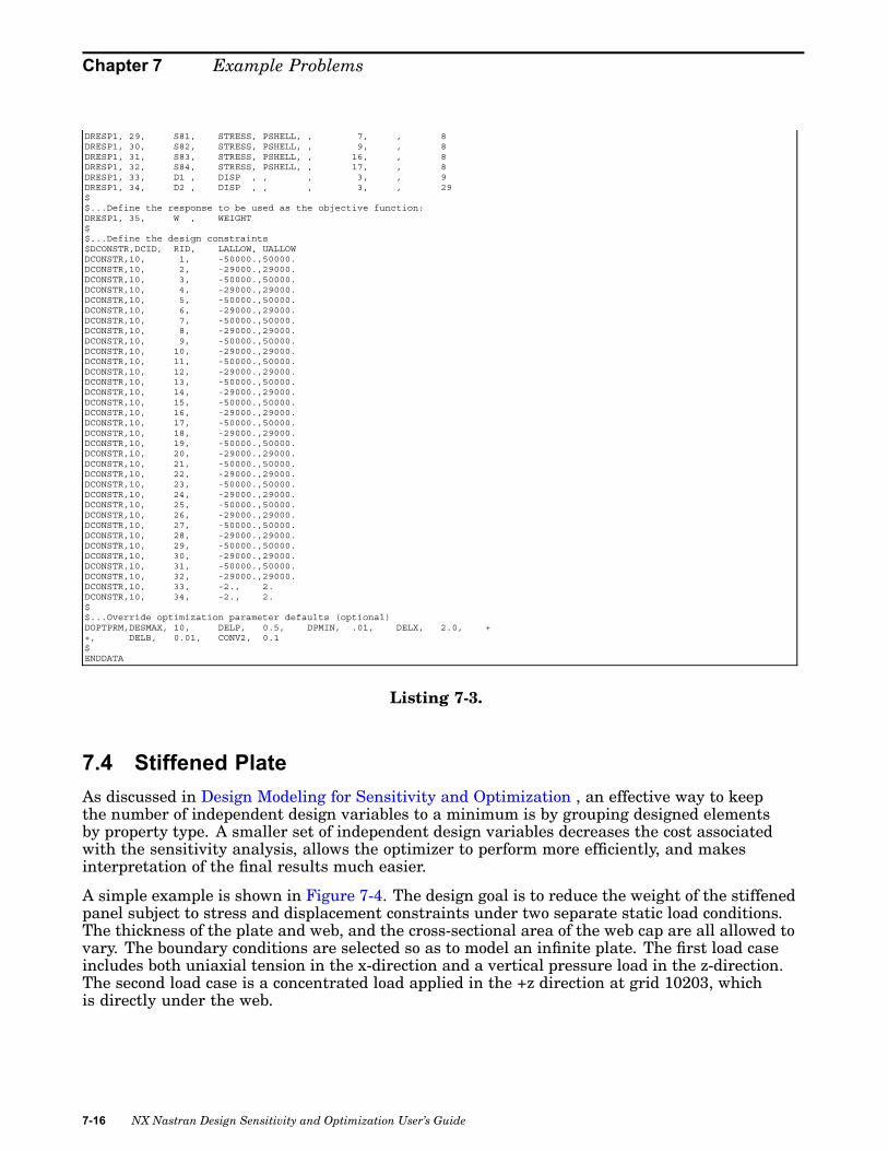
Chapter 7 Example Problems
DRESP1, 29, S81, STRESS, PSHELL, , 7, , 8DRESP1, 30, S82, STRESS, PSHELL, , 9, , 8DRESP1, 31, S83, STRESS, PSHELL, , 16, , 8DRESP1, 32, S84, STRESS, PSHELL, , 17, , 8DRESP1, 33, D1 , DISP , , , 3, , 9DRESP1, 34, D2 , DISP , , , 3, , 29$$...Define the response to be used as the objective function:DRESP1, 35, W , WEIGHT$$...Define the design constraints$DCONSTR,DCID, RID, LALLOW, UALLOWDCONSTR,10, 1, -50000.,50000.DCONSTR,10, 2, -29000.,29000.DCONSTR,10, 3, -50000.,50000.DCONSTR,10, 4, -29000.,29000.DCONSTR,10, 5, -50000.,50000.DCONSTR,10, 6, -29000.,29000.DCONSTR,10, 7, -50000.,50000.DCONSTR,10, 8, -29000.,29000.DCONSTR,10, 9, -50000.,50000.DCONSTR,10, 10, -29000.,29000.DCONSTR,10, 11, -50000.,50000.DCONSTR,10, 12, -29000.,29000.DCONSTR,10, 13, -50000.,50000.DCONSTR,10, 14, -29000.,29000.DCONSTR,10, 15, -50000.,50000.DCONSTR,10, 16, -29000.,29000.DCONSTR,10, 17, -50000.,50000.DCONSTR,10, 18, -29000.,29000.DCONSTR,10, 19, -50000.,50000.DCONSTR,10, 20, -29000.,29000.DCONSTR,10, 21, -50000.,50000.DCONSTR,10, 22, -29000.,29000.DCONSTR,10, 23, -50000.,50000.DCONSTR,10, 24, -29000.,29000.DCONSTR,10, 25, -50000.,50000.DCONSTR,10, 26, -29000.,29000.DCONSTR,10, 27, -50000.,50000.DCONSTR,10, 28, -29000.,29000.DCONSTR,10, 29, -50000.,50000.DCONSTR,10, 30, -29000.,29000.DCONSTR,10, 31, -50000.,50000.DCONSTR,10, 32, -29000.,29000.DCONSTR,10, 33, -2., 2.DCONSTR,10, 34, -2., 2.$$...Override optimization parameter defaults (optional)DOPTPRM,DESMAX, 10, DELP, 0.5, DPMIN, .01, DELX, 2.0, ++, DELB, 0.01, CONV2, 0.1$ENDDATA
Listing 7-3.
7.4 Stiffened PlateAs discussed in Design Modeling for Sensitivity and Optimization , an effective way to keepthe number of independent design variables to a minimum is by grouping designed elementsby property type. A smaller set of independent design variables decreases the cost associatedwith the sensitivity analysis, allows the optimizer to perform more efficiently, and makesinterpretation of the final results much easier.
A simple example is shown in Figure 7-4. The design goal is to reduce the weight of the stiffenedpanel subject to stress and displacement constraints under two separate static load conditions.The thickness of the plate and web, and the cross-sectional area of the web cap are all allowed tovary. The boundary conditions are selected so as to model an infinite plate. The first load caseincludes both uniaxial tension in the x-direction and a vertical pressure load in the z-direction.The second load case is a concentrated load applied in the +z direction at grid 10203, whichis directly under the web.
7-16 NX Nastran Design Sensitivity and Optimization User’s Guide

Example Problems
Figure 7-4. Stiffened Plate Model.
Analysis Model Description
16 CQUAD4 element to model uniform thickness base plate8 CQUAD4 elements to model the uniform thickness web4 CROD elements to model the uniform cross-sectional area web cap
Material: E = 1.0E7 psi
Poisson ratio = 0.33
Weight density = 0.283 lbs/in3
Loadings: Subcase 1: In-plane load of Nx = 1000 lbs/in
Uniform pressure load of 50 psi over the plate in the positivez-direction
Subcase 2: Lumped vertical load of 10,000 lbs at Grid 10203
Design Model Description
Objective: Structural weight minimization
Design variables: Plate thickness, web thickness, and web cap cross-sectional properties
Constraints:
NX Nastran Design Sensitivity and Optimization User’s Guide 7-17

Chapter 7 Example Problems
Strength: von Mises stress ≤ 25,000 psi at the centroid of plate elements forSubcase 1
Maximum axial stress ≤ 25,000 psi at both ends of rod elements forSubcase 2
Displacement: Vertical displacement at grid point 10302 for Subcase 1 ≤ 0.1 inches
Vertical displacement at grid point 10203 for Subcase 2 ≤ 0.03 inches
The DVPREL1 entries 1, 2, and 3 each express an analysis model property directly in termsof a given design variable:
Equation 7-4.
If the cap section is assumed to have a rectangular cross-section, then the other cross-sectionalproperties can be expressed directly in terms of the area Design Variable. Figure 7-5 shows arectangular cross section characterized by the dimensions b and h, with four stress recoverypoints C, D, E, and F.
Figure 7-5.
The initial area can be written in terms of the original dimensions as
7-18 NX Nastran Design Sensitivity and Optimization User’s Guide

Example Problems
Equation 7-5.
For a proportional change Δ in the cross-sectional dimensions b and h , the corresponding area is
Equation 7-6.
or
Equation 7-7.
To look at it another way, for a given change in the design variable, area, we immediately knowhow the underlying cross-sectional dimensions change. This can be used to express the changesin area moments of inertia in terms of Δ, or:
Equation 7-8.
where:
Equation 7-9.
and so on.
Since bending stresses in the web cap are to be used in the design model as constraints, thestress recovery points must move as the area changes. If not, then we fail to recover stressesat the outer corners of the cross section where bending stresses are greatest. For point C wehave, in terms of Δ:
NX Nastran Design Sensitivity and Optimization User’s Guide 7-19

Chapter 7 Example Problems
Equation 7-10.
and so on for the other stress recovery points, D, E, and F.
Since the above relations are nonlinear in the design variable x 3, we need to express these usingDVPREL2 Bulk Data entries. These entries provide the input arguments to the DEQATN entrieson which the preceding relations have been defined. In addition, the DTABLE Bulk Data entryhas been used to define constants that appear in the equations. We could have provided theseconstants directly on the DEQATN Bulk Data entries instead, but the loss of generality wouldhave required us to use additional equations.
In order for a structural response to be used either as an objective or a constraint, it first must beidentified on a DRESPi Bulk Data entry. The DRESP1 entries 1 and 2, for example, identify themaximum stress at ends A and B of a bar element. (Plot codes are used in the ATTA fields of theDRESP1 entry. For the BAR element, Item 7 is the maximum stress at end A, and Item14 isthe maximum stress at end B. See Appendix A of the NX Nastran Quick Reference Guide for alist of these plot codes.) The ATTi fields on these entries identify the property ID; here it is 3.DRESP1 number 1 indicates that the maximum end A stress for every BAR element in PBARgroup 3 is to be used in the design model for a total of four such responses. DRESP1 number 2identifies similar information for end B of the BAR elements.
Similarly, DRESP1 entries 3, 6, 9, and 12 identify the von Mises stresses at Z1 and Z2 for allelements in the web and in the plate. These responses are, in turn, constrained by the bounds setusing a corresponding set of DCONSTR entries (numbers 3, 6, 9, and 12).
From the summary of design cycle history, note that the initial constraint violation is greaterthan 100%. Even though the initial design is infeasible, the optimizer is able to obtain a feasibledesign after the second iteration. However, this is at the expense of additional structural masswith a weight increase to 16.4 lbs. from 5.8 lbs. Once a feasible design is achieved, the optimizercan begin trying to reduce the weight, achieving a final weight of 7.9 lbs. Of course, this designis still heavier than the original structure (by almost 40%), yet that design did not satisfy theperformance constraints whereas this one does.
***** NORMAL CONVERGENCE CRITERIA SATISFIED ***** (HARD CONVERGENCE DECISION LOGIC)**************************************************************************************
CONVERGENCE ACHIEVED BASED ON THE FOLLOWING CRITERIA(HARD CONVERGENCE DECISION LOGIC)
RELATIVE CHANGE IN OBJECTIVE 0.0000E+00 MUST BE LESS THAN 1.0000E-03OR ABSOLUTE CHANGE IN OBJECTIVE 0.0000E+00 MUST BE LESS THAN 1.0000E-02
--- AND ---MAXIMUM CONSTRAINT VALUE 1.8636E-03 MUST BE LESS THAN 5.0000E-03
(CONVERGENCE TO A FEASIBLE DESIGN)--- OR ---
MAXIMUM OF RELATIVE PROP. CHANGES 0.0000E+00 MUST BE LESS THAN 1.0000E-03AND MAXIMUM OF RELATIVE D.V. CHANGES 0.0000E+00 MUST BE LESS THAN 1.0000E-03
(CONVERGENCE TO A BEST COMPROMISE INFEASIBLE DESIGN)**************************************************************************************
7-20 NX Nastran Design Sensitivity and Optimization User’s Guide

Example Problems
***************************************************************S U M M A R Y O F D E S I G N C Y C L E H I S T O R Y***************************************************************
(HARD CONVERGENCE ACHIEVED)(SOFT CONVERGENCE ACHIEVED)
NUMBER OF FINITE ELEMENT ANALYSES COMPLETED 8NUMBER OF OPTIMIZATIONS W.R.T. APPROXIMATE MODELS 7
OBJECTIVE AND MAXIMUM CONSTRAINT HISTORY---------------------------------------------------------------------------------------------------------------
OBJECTIVE FROM OBJECTIVE FROM FRACTIONAL ERROR MAXIMUM VALUE ROW OFCYCLE APPROXIMATE EXACT OF OF MAXIMUMNUMBER OPTIMIZATION ANALYSIS APPROXIMATION CONSTRAINT CONSTRAINT
---------------------------------------------------------------------------------------------------------------INITIAL 5.784520E+00 1.311878E+00 10
1 1.122267E+01 1.122355E+01 -7.868297E-05 4.089278E-01 22 1.636887E+01 1.636941E+01 -3.285838E-05 -1.610547E-03 23 1.294620E+01 1.294636E+01 -1.259646E-05 -8.604820E-02 14 8.748927E+00 8.751337E+00 -2.753791E-04 1.988992E-02 105 7.379158E+00 7.379156E+00 3.230973E-07 9.885500E-02 216 7.948771E+00 7.948517E+00 3.197505E-05 1.863594E-03 197 7.948491E+00 7.948517E+00 -3.359479E-06 1.863594E-03 19
---------------------------------------------------------------------------------------------------------------
DESIGN VARIABLE HISTORY--------------------------------------------------------------------------------------------------------------------------------
INTERNAL | EXTERNAL | |DV. ID. | DV. ID. | LABEL | INITIAL : 1 : 2 : 3 : 4 : 5 :
--------------------------------------------------------------------------------------------------------------------------------1 | 1 | T-PLATE | 1.5000E-01 : 3.0000E-01 : 4.4321E-01 : 2.8106E-01 : 1.4038E-01 : 1.0879E-01 :2 | 2 | T-WEB | 2.0000E-01 : 4.0000E-01 : 6.1265E-01 : 8.4962E-01 : 8.2809E-01 : 7.5169E-01 :3 | 3 | A-BAR | 1.4400E-01 : 1.6592E-01 : 1.2682E-01 : 6.4814E-02 : 3.2407E-02 : 1.6165E-02 :
--------------------------------------------------------------------------------------------------------------------------------INTERNAL | EXTERNAL | |DV. ID. | DV. ID. | LABEL | 6 : 7 : 8 : 9 : 10 : 11 :
--------------------------------------------------------------------------------------------------------------------------------1 | 1 | T-PLATE | 1.1180E-01 : 1.1180E-01 :2 | 2 | T-WEB | 8.3723E-01 : 8.3723E-01 :3 | 3 | A-BAR | 1.6165E-02 : 1.6165E-02 :
--------------------------------------------------------------------------------------------------------------------------------*** USER INFORMATION MESSAGE 6464 (DOM12E)
RUN TERMINATED DUE TO HARD CONVERGENCE TO A UNIQUE OPTIMUM AT CYCLE NUMBER = 7.
ID UGS, D200X7TIME 10SOL 200 $ OPTIMIZATIONCEND$TITLE = STATIC ANALYSIS OF A STIFFENED PLATEECHO = UNSORTDISP = ALLSTRESS = ALLSPC = 1ANALYSIS = STATICSDESOBJ(MIN) = 15 $ OBJECTIVE FUNCTION DEFINITION$ (MIN IS THE DEFAULT)SUBCASE 1
LABEL = LOAD CONDITION 1LOAD = 1DESSUB = 100 $ CONSTRAINT DEFININITION
SUBCASE 2LABEL = LOAD CONDITION 2LOAD = 2DESSUB = 200 $ CONSTRAINT DEFININITION
BEGIN BULK$$------------------------------------------------------------------------$ ANALYSIS MODEL:$------------------------------------------------------------------------$GRID, 10000, , 0.0, 0.0, 0.0GRID, 10001, , 2.5, 0.0, 0.0GRID, 10002, , 5.0, 0.0, 0.0GRID, 10003, , 7.5, 0.0, 0.0GRID, 10004, , 10.0, 0.0, 0.0GRID, 10100, , 0.0, 2.5, 0.0GRID, 10101, , 2.5, 2.5, 0.0GRID, 10102, , 5.0, 2.5, 0.0GRID, 10103, , 7.5, 2.5, 0.0GRID, 10104, , 10.0, 2.5, 0.0GRID, 10200, , 0.0, 5.0, 0.0GRID, 10201, , 2.5, 5.0, 0.0GRID, 10202, , 5.0, 5.0, 0.0GRID, 10203, , 7.5, 5.0, 0.0GRID, 10204, , 10.0, 5.0, 0.0GRID, 10300, , 0.0, 7.5, 0.0GRID, 10301, , 2.5, 7.5, 0.0GRID, 10302, , 5.0, 7.5, 0.0GRID, 10303, , 7.5, 7.5, 0.0GRID, 10304, , 10.0, 7.5, 0.0GRID, 10400, , 0.0, 10.0, 0.0
NX Nastran Design Sensitivity and Optimization User’s Guide 7-21
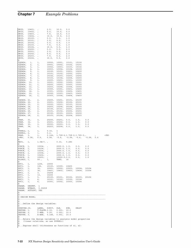
Chapter 7 Example Problems
GRID, 10401, , 2.5, 10.0, 0.0GRID, 10402, , 5.0, 10.0, 0.0GRID, 10403, , 7.5, 10.0, 0.0GRID, 10404, , 10.0, 10.0, 0.0GRID, 20100, , 0.0, 5.0, 1.0GRID, 20101, , 2.5, 5.0, 1.0GRID, 20102, , 5.0, 5.0, 1.0GRID, 20103, , 7.5, 5.0, 1.0GRID, 20104, , 10.0, 5.0, 1.0GRID, 20200, , 0.0, 5.0, 2.0GRID, 20201, , 2.5, 5.0, 2.0GRID, 20202, , 5.0, 5.0, 2.0GRID, 20203, , 7.5, 5.0, 2.0GRID, 20204, , 10.0, 5.0, 2.0$CQUAD4, 1, 1, 10000, 10001, 10101, 10100CQUAD4, 2, 1, 10001, 10002, 10102, 10101CQUAD4, 3, 1, 10002, 10003, 10103, 10102CQUAD4, 4, 1, 10003, 10004, 10104, 10103CQUAD4, 5, 1, 10100, 10101, 10201, 10200CQUAD4, 6, 1, 10101, 10102, 10202, 10201CQUAD4, 7, 1, 10102, 10103, 10203, 10202CQUAD4, 8, 1, 10103, 10104, 10204, 10203CQUAD4, 9, 1, 10200, 10201, 10301, 10300CQUAD4, 10, 1, 10201, 10202, 10302, 10301CQUAD4, 11, 1, 10202, 10203, 10303, 10302CQUAD4, 12, 1, 10203, 10204, 10304, 10303CQUAD4, 13, 1, 10300, 10301, 10401, 10400CQUAD4, 14, 1, 10301, 10302, 10402, 10401CQUAD4, 15, 1, 10302, 10303, 10403, 10402CQUAD4, 16, 1, 10303, 10304, 10404, 10403$CQUAD4, 21, 2, 10200, 10201, 20101, 20100CQUAD4, 22, 2, 10201, 10202, 20102, 20101CQUAD4, 23, 2, 10202, 10203, 20103, 20102CQUAD4, 24, 2, 10203, 10204, 20104, 20103CQUAD4, 25, 2, 20100, 20101, 20201, 20200CQUAD4, 26, 2, 20101, 20102, 20202, 20201CQUAD4, 27, 2, 20102, 20103, 20203, 20202CQUAD4, 28, 2, 20103, 20104, 20204, 20203$CBAR, 31, 3, 20200, 20201, 0.0, 1.0, 0.0CBAR, 32, 3, 20201, 20202, 0.0, 1.0, 0.0CBAR, 33, 3, 20202, 20203, 0.0, 1.0, 0.0CBAR, 34, 3, 20203, 20204, 0.0, 1.0, 0.0$PSHELL, 1, 1, 0.15, 1PSHELL, 2, 1, 0.2, 1PBAR, 3, 1, 0.144, 1.728-4,1.728-2,1.745-2,, , +PB3+PB3, 0.06, 0.6, 0.06, -0.6, -0.06, -0.6, -0.06, 0.6$MAT1, 1, 1.0E+7, , 0.33, 0.283$FORCE, 1, 10004, , 2000.0, 1.0, 0.0, 0.0FORCE, 1, 10104, , 2000.0, 1.0, 0.0, 0.0FORCE, 1, 10204, , 2000.0, 1.0, 0.0, 0.0FORCE, 1, 10304, , 2000.0, 1.0, 0.0, 0.0FORCE, 1, 10404, , 2000.0, 1.0, 0.0, 0.0FORCE, 2, 10203, , 10000.0,0.0, 0.0, 1.0PLOAD2, 1, 50., 1, THRU, 16$SPC1, 1, 1236, 10000SPC1, 1, 136, 10100, 10300, 10400SPC1, 1, 36, 10001, 10002, 10003, 10004, 10104SPC1, 1, 36, 10401, 10402, 10403, 10404, 10304SPC1, 1, 3, 10204SPC1, 1, 13, 10200SPC1, 1, 5, 20100, 20101, 20102, 20103, 20104SPC1, 1, 6, 10101, 10102, 10103, 10104SPC1, 1, 6, 10301, 10302, 10303, 10304$PARAM, GRDPNT, 1PARAM, WTMASS, 0.00259PARAM, AUTOSPC, YES$$------------------------------------------------------------------------$ DESIGN MODEL:$------------------------------------------------------------------------$$...Define the design variables:$$DESVAR,ID, LABEL, XINIT, XLB, XUB, DELXVDESVAR, 1, T-PLATE,0.15, 0.001, 10.0DESVAR, 2, T-WEB, 0.20, 0.001, 10.0DESVAR, 3, A-BAR, 0.144, 0.001, 10.0$$...Relate the design variables to analysis model properties$ (linear relations, so use DVPREL1)$$...Express shell thicknesses as functions of x1, x2:
7-22 NX Nastran Design Sensitivity and Optimization User’s Guide

Example Problems
$DVPREL1,ID, TYPE, PID, FID, PMIN, PMAX, C0, , +$+, DVIDD1, COEF1, DVID2, COEF2, ...DVPREL1,1, PSHELL, 1, 4, 0.01, , , , +DP1+DP1, 1, 1.0DVPREL1,2, PSHELL, 2, 4, 0.01, , , , +DP2+DP2, 2, 1.0$$...Express bar cross sectional area as a function of x3:DVPREL1,3, PBAR, 3, 4, 0.01, , , , +DP3+DP3, 3, 1.0$$...Proportionally relate bar’s I1, I2, I12 to changes in area (x3):$ (nonlinear relations require use of DVPREL2+DEQATN)$DVPREL2,ID, TYPE, PID, FID, PMIN, PMAX, EQID, , +$+, DESVAR,DVID1, DVID2, ..., , , , , +$+, DTABLE,CID1, CID2, ...DVPREL2,11, PBAR, 3, 5, 1.0-6, , 101, , ++, DESVAR, 3, , , , , , , ++, DTABLE, X3INIT, I1INITDEQATN 101 I1(X3,X3INIT,I1INIT) = I1INIT ;
DELTA = SQRT(X3/X3INIT) ;I1NEW = I1*DELTA**4
DVPREL2,12, PBAR, 3, 6, 1.0-6, , 102, , ++, DESVAR, 3, , , , , , , ++, DTABLE, X3INIT, I2INITDEQATN 102 I2(X3,X3INIT,I2INIT) = I2INIT ;
DELTA = SQRT(X3/X3INIT) ;I2NEW = I2*DELTA**4
DVPREL2,13, PBAR, 3, 7, 1.0-6, , 103, , ++, DESVAR, 3, , , , , , , ++, DTABLE, X3INIT, I12INITDEQATN 103 I12(X3,X3INIT,I12INIT) = I12INIT ;
DELTA = SQRT(X3/X3INIT) ;I12NEW = I12*DELTA**4
$$...Modify stress recovery points accordingly:DVPREL2,14, PBAR, 3, 12, , , 104, , ++, DESVAR, 3, , , , , , , ++, DTABLE, X3INIT, CYINITDVPREL2,15, PBAR, 3, 13, , , 104, , ++, DESVAR, 3, , , , , , , ++, DTABLE, X3INIT, CZINITDVPREL2,16, PBAR, 3, 14, , , 104, , ++, DESVAR, 3, , , , , , , ++, DTABLE, X3INIT, DYINITDVPREL2,17, PBAR, 3, 15, -1.0, , 104, , ++, DESVAR, 3, , , , , , , ++, DTABLE, X3INIT, DZINITDVPREL2,18, PBAR, 3, 16, -1.0, , 104, , ++, DESVAR, 3, , , , , , , ++, DTABLE, X3INIT, EYINITDVPREL2,19, PBAR, 3, 17, -1.0, , 104, , ++, DESVAR, 3, , , , , , , ++, DTABLE, X3INIT, EZINITDVPREL2,20, PBAR, 3, 18, -1.0, , 104, , ++, DESVAR, 3, , , , , , , ++, DTABLE, X3INIT, FYINITDVPREL2,21, PBAR, 3, 19, , , 104, , ++, DESVAR, 3, , , , , , , ++, DTABLE, X3INIT, FZINIT$$...Equation for stress recovery points:DEQATN 104 NEWPOINT(X3,X3INIT,POINT) = POINT*SQRT(X3/X3INIT)$$...Table constants for all equations:DTABLE, X3INIT, 0.144, I1INIT, 1.728-4,I2INIT, 1.728-2,I12INIT,1.745-2,++, CYINIT, 0.06, CZINIT, 0.6, DYINIT, 0.06, DZINIT, -0.6, ++, EYINIT, -0.06, EZINIT, -0.6, FYINIT, -0.06, FZINIT, 0.6$$...Identify the design responses:$$DRESP1,ID, LABEL, RTYPE, PTYPE, REGION, ATTA, ATTB, ATT1, +$+, ATT2, ...DRESP1, 1, SBARA, STRESS, PBAR, , 7, , 3DRESP1, 2, SBARB, STRESS, PBAR, , 14, , 3DRESP1, 3, S13, STRESS, PSHELL, , 9, , 1DRESP1, 6, S16, STRESS, PSHELL, , 17, , 1DRESP1, 9, S23, STRESS, PSHELL, , 9, , 2DRESP1, 12, S26, STRESS, PSHELL, , 17, , 2DRESP1, 13, D1, DISP, , , 3, , 10302DRESP1, 14, D2, DISP, , , 3, , 10203DRESP1, 15, W, WEIGHT$$...Place bounds on the responses:$$DCONSTR,DCID, RID, LALLOW, UALLOWDCONSTR, 10, 1, -25000.,25000.DCONSTR, 10, 2, -25000.,25000.DCONSTR, 10, 3, -25000.,25000.DCONSTR, 10, 6, -25000.,25000.
NX Nastran Design Sensitivity and Optimization User’s Guide 7-23

Chapter 7 Example Problems
DCONSTR, 10, 9, -25000.,25000.DCONSTR, 10, 12, -25000.,25000.DCONSTR, 20, 13, -0.1, 0.1DCONSTR, 30, 14, -0.03, 0.03$$DCONADD,DCID, DC1, DC2, ...DCONADD, 100, 10, 20 $ summed constraint set for subcase 1DCONADD, 200, 10, 30 $ summed constraint set for subcase 2$$...Optional override of optimization control parameters:$DOPTPRM,IPRINT, 1, DESMAX, 20, DELP, 0.5, P1, 1, ++, P2, 15$ (DELP=0.5 allows larger moves, thus overcoming constraint$ violations quicker)$ENDDATA
Listing 7-4.
7.5 Shape Optimization of a CulvertThis example considers shape optimization using the direct input of shapes method.
In order to use this method, sets of displacement vectors are first generated using a separateauxiliary model analysis. These displacement vectors are then DBLOCATEd in a subsequentdesign optimization run and used to generate a set of shape basis vectors. The optimizer thenseeks to find the best combination of these shape basis vectors.
Problem DescriptionFigure 7-6 shows the finite element model of one half of a symmetric culvert structure.(Symmetry exists with respect to the y-axis.) The structure is made of steel, and has beenmodeled using CQUAD4 elements in plane strain. This example has been taken from A. D.Belegundu, and S. D. Rajan, “Shape Optimal Design Using Isoparametric Elements”, Proceedingsof 29th AIAA/ASME/ASCE/AHS/ASC Structures, Dynamics, and Materials Conference, pp.696–701, Williamsburg, VA, April 18–20, 1988.
7-24 NX Nastran Design Sensitivity and Optimization User’s Guide

Example Problems
Figure 7-6. Initial Culvert Design.
With the bottom surface fixed, pressure loads are applied on the top surface. The design taskis to minimize the volume of the structure by changing the shape of the initially circular hole,subject to von Mises stress constraints over the interior.
Modeling Considerations
The process of shape basis vector generation is closely associated with the nature of the designproblem itself. For example, since the goal here is weight minimization, the shape basis vectorsmust clearly be able to reduce the volume of the structure. Were they to simply redistributematerial, the weight would not change and the optimizer would be able to make little progress.
Furthermore, since the redesign is subject to von Mises stresses, we can use the initial stressdistribution to help us in the selection of appropriate basis vectors. This is also shown in Figure7-6. Here we note that the maximum von Mises stresses occur around the lower portion ofthe circular hole. The stresses are not equally distributed, either. This tells us that a circularboundary does not provide the optimal design. Thus, our shape basis vectors must containother than just radial components.
We also need to decide how many design variables (or shape basis vectors) are needed. Thedecision is not unique because the selection can be affected by experience, various functionaland manufacturing requirements, or aesthetic requirements. However, the shape basis vectorsshould yield as much generality as possible, consistent with our design goals.
Creation of Auxiliary Model, and Generation of Basis Vectors
The top left frame in Figure 7-7 shows the auxiliary model geometry and boundary conditions.Note that it has the same geometry as the primary structure (Figure 7-6), but with differentboundary and loading conditions. The input data file for this model is given in Listing 7-5.
NX Nastran Design Sensitivity and Optimization User’s Guide 7-25

Chapter 7 Example Problems
Figure 7-7. Auxiliary Model.
Outside edges of the culvert are fixed in the auxiliary model to satisfy straight edge requirements.Grid points 1, 2, 3 on the bottom are allowed to move in the x-direction and grid points 13, 20,27 on the symmetry line can move along the y-direction. Grids 5, 9, 14, 15, and 16 on the holeboundary are allowed to move as well. Along this hole boundary, six CBAR elements havebeen added to help smooth the applied loading effects. (It is important to allow z-rotationsalong this boundary.)
To generate a set of displacements to be used as basis vectors, we can statically load each grid ina direction normal to the boundary as shown in Figure 7-7. Note from Listing 7-5 that this canbe performed in Solution 101 (or in Solution 200, with OPTEXIT = 2). This will result in sevendisplacement vectors, one corresponding to each load case. Three of these vectors are also shownin Figure 7-7. Each arrow on a plot indicates that the deformation is due to a concentrated force.
Design Optimization Input
In the optimization run, the displacement matrix containing the seven displacement vectors fromthe Auxiliary Model analysis is retrieved using the DBLOCATE statement. The optimizationinput file is shown in Listing 7-7.
Since each shape basis vector is defined in terms of a single displacement vector, seven DESVARand DVSHAP entries are used to define seven shape basis vectors. The seven DVSHAP entryscaling factors have been selected such that the maximum component of each shape basis vectoris unity. For example, DVSHAP entry number 1 identifies the first shape basis vector in terms ofthe first DBLOCATE’d displacement vector (1 in field 3). The 1 in field 2 indicates that designvariable number 1 is to be the multiplier of this vector. Furthermore, since the maximumcomponent of this vector is 1.0/66.773 (as determined from a manual inspection of the data), thescaling factor has been given as 66.773, effectively unit normalizing the vector.
7-26 NX Nastran Design Sensitivity and Optimization User’s Guide

Example Problems
Each design variable acts as a multiplying coefficient of a shape basis vector. Initial values aresomewhat arbitrary and have been selected as 3.0 here. However, when combined with 20%allowable move limits (0.2 in field 7 of the DESVAR entries), it can be seen that part of thereason for the choice is that these initial values provide for reasonable move limits on the initialdesign. Lower and upper limits of -1.0E6 and +1.0E6 indicate that the design variables are to beconsidered effectively unbounded during optimization.
The final shape after six design cycles is plotted in Figure 7-8 (bottom half) with thecorresponding stress contour plot of the deformed structure (top half). Note the favorabledistribution of von Mises stresses for the final shape. The volume of the culvert has been reducedby about 20% while the strength constraint is satisfied.
Figure 7-8. Final Culvert Design.
ID,AUX1,VT100 $FEB 10,1990TIME 10SOL 101CENDTITLE=Culvert Example Using External Auxiliary ModelSUBTITLE=The External Auxiliary ModelSPC=25$$ seven load cases$SUBCASE 1LOAD=100DISP=ALL
SUBCASE 2LOAD=101DISP=ALL
SUBCASE 3LOAD=102DISP=ALL
SUBCASE 4LOAD=103DISP=ALL
SUBCASE 5LOAD=104DISP=ALL
SUBCASE 6LOAD=105DISP=ALL
SUBCASE 7LOAD=106DISP=ALL
BEGIN BULK
NX Nastran Design Sensitivity and Optimization User’s Guide 7-27

Chapter 7 Example Problems
PARAM,POST,0param,newseq,-1$$ The same GRID and CQUAD4 entries as the primary structure$GRID, 1,, 3.00000, 0.00000,.00GRID, 2,, 4.00000, 0.00000,.00GRID, 3,, 5.00000, 0.00000,.00
. . . . .
. . . . .(see optimization input file). . . . .. . . . .
GRID, 38,, 2.00000, 5.19600,.00GRID, 39,, 2.50000, 5.19600,.00GRID, 40,, 3.00000, 5.19600,.00CQUAD4, 1,101, 1, 2, 6, 5CQUAD4, 2,101, 2, 3, 7, 6CQUAD4, 3,101, 3, 4, 8, 7
. . . . . . .
. . . . . . .(see optimization input file). . . . . . .. . . . . . .
CQUAD4, 25,101, 30, 31, 38, 37CQUAD4, 26,101, 31, 32, 39, 38CQUAD4, 27,101, 32, 33, 40, 39PSHELL,101,102,.44MAT1,102,2.+7,,.3$$ Additional CBAR elements maintain smoothness of the circular boundary$CBAR,31,1,13,14,,1.0CBAR,32,1,14,15,,1.0CBAR,33,1,15,16,,1.0CBAR,34,1,16, 9,,1.0CBAR,35,1, 9, 5,,1.0CBAR,36,1,5 , 1,,1.0PBAR 1 102 20.0 1.0 1.0$$ Seven load cases$FORCE,100,13,0,1.e5,0.,1.,0.FORCE,101,14,0,1.e5,0.259,.9659FORCE,102,15,0,1.e5,0.5,0.866,0.0FORCE,103,16,0,1.e5,1.,1.,0.FORCE,104,9,0,1.e5,0.866,0.5,0.0FORCE,105,5,0,1.e5,0.9659,0.259FORCE,106,1,0,1.e5,1.,0.,0.$$ Boundary conditions satisfy functional and manufacturing requirements$SPC1,25,345,1,THRU,40SPC1,25,6,2,THRU,4SPC1,25,6,6,THRU,8SPC1,25,6,10,THRU,12SPC1,25,6,17,THRU,19SPC1,25,6,20,THRU,26SPC1,25,6,27,THRU,33SPC1,25,6,34,THRU,40SPC1,25,12,33,THRU,40SPC1,25,12,4,8,12,19,26SPC1,25,1,13,20,27SPC1,25,2,1,2,3ENDDATA
Listing 7-5.
$$ FMS section for retrieving the auxiliary displacement matrix$assign f1_aux=’culvert1.MASTER’dblocate datablk=(ug/ugd,geom1/geom1d,geom2/geom2d) ,logical=f1_aux
SOL 200 $TIME 100CENDTITLE=CULVERT EXAMPLE USING EXTERNAL AUXILIARY STRUCTURESUBTITLE=THE PRIMARY STRUCTUREANALYSIS = STATICSSPC=25LOAD=1DISP=ALLSTRESS=allDESSUB = 10desobj = 5
BEGIN BULKPARAM,POST,0
7-28 NX Nastran Design Sensitivity and Optimization User’s Guide

Example Problems
PARAM,CDIF,NO$ PARAM,optexit,4PARAM,NEWSEQ,-1GRID, 1,, 3.00000, 0.00000,.00GRID, 2,, 4.00000, 0.00000,.00GRID, 3,, 5.00000, 0.00000,.00GRID, 4,, 6.00000, 0.00000,.00GRID, 5,, 2.89464, 0.78478,.00GRID, 6,, 3.79369, 0.75885,.00GRID, 7,, 4.69274, 0.73293,.00GRID, 8,, 5.59178, 0.70700,.00GRID, 9,, 2.60164, 1.49178,.00GRID, 10,, 3.46229, 1.46585,.00GRID, 11,, 4.32293, 1.43993,.00GRID, 12,, 5.18357, 1.41400,.00GRID, 13,, 0.00000, 3.00000,.00GRID, 14,, 0.78478, 2.89464,.00GRID, 15,, 1.49178, 2.60164,.00GRID, 16,, 2.12100, 2.12100,.00GRID, 17,, 3.00578, 2.12100,.00GRID, 18,, 3.89057, 2.12100,.00GRID, 19,, 4.77535, 2.12100,.00GRID, 20,, 0.00000, 3.73200,.00GRID, 21,, 0.68985, 3.66176,.00GRID, 22,, 1.32785, 3.46643,.00GRID, 23,, 1.91400, 3.14600,.00GRID, 24,, 2.67052, 3.14600,.00GRID, 25,, 3.42704, 3.14600,.00GRID, 26,, 4.18357, 3.14600,.00GRID, 27,, 0.00000, 4.46400,.00GRID, 28,, 0.59493, 4.42888,.00GRID, 29,, 1.16393, 4.33122,.00GRID, 30,, 1.70700, 4.17100,.00GRID, 31,, 2.33526, 4.17100,.00GRID, 32,, 2.96352, 4.17100,.00GRID, 33,, 3.59178, 4.17100,.00GRID, 34,, 0.00000, 5.19600,.00GRID, 35,, 0.50000, 5.19600,.00GRID, 36,, 1.00000, 5.19600,.00GRID, 37,, 1.50000, 5.19600,.00GRID, 38,, 2.00000, 5.19600,.00GRID, 39,, 2.50000, 5.19600,.00GRID, 40,, 3.00000, 5.19600,.00CQUAD4, 1,101, 1, 2, 6, 5CQUAD4, 2,101, 2, 3, 7, 6CQUAD4, 3,101, 3, 4, 8, 7CQUAD4, 4,101, 5, 6, 10, 9CQUAD4, 5,101, 6, 7, 11, 10CQUAD4, 6,101, 7, 8, 12, 11CQUAD4, 7,101, 9, 10, 17, 16CQUAD4, 8,101, 10, 11, 18, 17CQUAD4, 9,101, 11, 12, 19, 18CQUAD4, 10,101, 13, 14, 21, 20CQUAD4, 11,101, 14, 15, 22, 21CQUAD4, 12,101, 15, 16, 23, 22CQUAD4, 13,101, 20, 21, 28, 27CQUAD4, 14,101, 21, 22, 29, 28CQUAD4, 15,101, 22, 23, 30, 29CQUAD4, 16,101, 27, 28, 35, 34CQUAD4, 17,101, 28, 29, 36, 35CQUAD4, 18,101, 29, 30, 37, 36CQUAD4, 19,101, 16, 17, 24, 23CQUAD4, 20,101, 17, 18, 25, 24CQUAD4, 21,101, 18, 19, 26, 25CQUAD4, 22,101, 23, 24, 31, 30CQUAD4, 23,101, 24, 25, 32, 31CQUAD4, 24,101, 25, 26, 33, 32CQUAD4, 25,101, 30, 31, 38, 37CQUAD4, 26,101, 31, 32, 39, 38CQUAD4, 27,101, 32, 33, 40, 39FORCE 1 34 0 1250. -1.FORCE 1 35 0 2500. -1.FORCE 1 36 0 2500. -1.FORCE 1 37 0 2500. -1.FORCE 1 38 0 2500. -1.FORCE 1 39 0 2500.00 -1.FORCE 1 40 0 1250. -1.PSHELL,101,102,.44MAT1,102,2.+7,,.3,0.731-3SPC1,25,3456,1,THRU,40SPC1,25,12,1,THRU,4SPC1,25,1,13,20,27,34$$ design model$desvar 1 b1 3. -1.e6 1.e6 .2desvar 2 b1 3. -1.e6 1.e6 .2desvar 3 b3 3. -1.e6 1.e6 .2desvar 4 b4 3. -1.e6 1.e6 .2desvar 5 b5 3. -1.e6 1.e6 .2
NX Nastran Design Sensitivity and Optimization User’s Guide 7-29
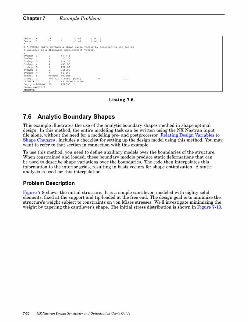
Chapter 7 Example Problems
desvar 6 b6 3. -1.e6 1.e6 .2desvar 7 b7 3. -1.e6 1.e6 .2$$ A DVSHAP entry defines a shape basis vector by associating one design$ variable to a dblocated displacement vector.$dvshap 1 1 66.773dvshap 2 2 117.35dvshap 3 3 216.33dvshap 4 4 443.55dvshap 5 5 220.89dvshap 6 6 115.69dvshap 7 7 65.669dresp1 5 volume volumedresp1 2 von-mis stress pshell 9 101DCONSTR 10 2 -3.100e43.100e4doptprm DESMAX 25 APRCOD 1param,nasprt,1ENDDATA
Listing 7-6.
7.6 Analytic Boundary ShapesThis example illustrates the use of the analytic boundary shapes method in shape optimaldesign. In this method, the entire modeling task can be written using the NX Nastran inputfile alone, without the need for a modeling pre- and postprocessor. Relating Design Variables toShape Changes , includes a checklist for setting up the design model using this method. You maywant to refer to that section in connection with this example.
To use this method, you need to define auxiliary models over the boundaries of the structure.When constrained and loaded, these boundary models produce static deformations that canbe used to describe shape variations over the boundaries. The code then interpolates thisinformation to the interior grids, resulting in basis vectors for shape optimization. A staticanalysis is used for this interpolation.
Problem DescriptionFigure 7-9 shows the initial structure. It is a simple cantilever, modeled with eighty solidelements, fixed at the support and tip-loaded at the free end. The design goal is to minimize thestructure’s weight subject to constraints on von Mises stresses. We’ll investigate minimizing theweight by tapering the cantilever’s shape. The initial stress distribution is shown in Figure 7-10.
7-30 NX Nastran Design Sensitivity and Optimization User’s Guide

Example Problems
Figure 7-9. Solid Cantilever.
Figure 7-10. Solid Cantilever - Initial Stress Distribution.
Since the cantilever is oriented and loaded in an x-z plane, removing material from the upperand lower surfaces is an effective way to reduce the weight, tapering the cantilever from its rootto its tip. Basis vectors describing this characteristic shape can be easily generated using theanalytic boundary shapes method.
NX Nastran Design Sensitivity and Optimization User’s Guide 7-31

Chapter 7 Example Problems
Boundary Shape Changes Using Auxiliary Boundary Models
Figure 7-11 shows the auxiliary boundary models that can be used to generate these shapes.These disjoint models, one for the upper surface and one for the lower, are built using QUAD4elements. When fixed at the root and loaded at the tip, each generates a cubic displacementvariation over its length.
Figure 7-11. Auxiliary Boundary Models.
Listing 7-8 is an abbreviated input file for the combined analysis and optimization of the primarystructure, and the auxiliary boundary model specification. The complete file can be found in theTest Problem Library as D200AM3.DAT. The primary model definition is similar to that of otherNX Nastran input files for static analysis shown in this guide, so its description will be deferredhere. The optimization-related input for the primary structure will be described shortly.
Turning first to the auxiliary boundary model specification, we see that these boundary modelsare defined in a special Bulk Data Section, appearing after the Bulk Data for the primary model.The statement, BEGIN BULK AUXMODEL = 1, is used to indicate the beginning of this section.This section essentially defines three components of the model: its connectivity, its loads, and itsboundary conditions. This is just like any other NX .Nastran model for static analysis.
The auxiliary boundary model connectivity is defined using CQUAD4 elements. The geometryshould not be redefined, since the primary model geometry is used. (If necessary, additional gridscan be included. For example, an additional grid may be necessary for use as a rigid elementconnection point. This grid should then appear in this Bulk Data Section.)
The structure is constrained using two SPC sets, 200 and 300. Each set corresponds to twoseparate loading conditions: one an enforced tip displacement in the +z direction for the lowersurface, the other an enforced tip displacement in the -z direction for the upper surface. Theseare defined using SPCD sets 220 and 330, respectively.
7-32 NX Nastran Design Sensitivity and Optimization User’s Guide

Example Problems
The Case Control for these models appears after the primary model Case Control, in a sectionbeginning with the label, AUXCASE. Each subcase selects one of the two SPCD-defined loads,using a different boundary condition for each. Static loading is always assumed for theseauxiliary model analyses.
The results of these two analyses are sets of displacement vectors, which essentially interpolatethe tip displacement along the length of each "plate." This smooth shape interpolation is nowquite useful for describing shape changes over the Primary Structure’s boundary. However,these boundary displacements must still be interpolated over the structure’s interior in orderto form shape basis vectors for the entire structure. This is achieved in the primary modelsection of the Bulk Data.
Shape Changes over the Interior
BNDGRID entries provide the boundary conditions for the shape interpolation steps. Therelation between BNDGRID entries and the auxiliary boundary model solutions is similar tothat of SPC’s and SPCD’s. The auxiliary boundary model solutions are imposed as enforceddisplacements on the primary structure. This is like an SPCD. These displacement degrees offreedom must be present on BNDGRID entries, as with SPC entries. Degrees of freedom listedon the BNDGRID entries are either enforced or fixed, depending on whether or not an auxiliaryboundary model solution exists for them. All other degrees of freedom are considered "free," andare solved for in the interpolation.
For example, grids 143, 154, and 165 are located at the tip of the upper surface (see Figure 7-9).Their displacement components are determined from the auxiliary model analysis. This isindicated by using a BNDGRID entry with a translational component of 123 given for each ofthese grids (see listing 7–7).
In contrast, the displacements at grids 110, 121, and 132, located directly below the previous setof grids, must be solved for during the interpolation phase. Since we want to allow the tip of thebeam to narrow, the z displacement component must not be fixed. In contrast, all must be fixedin the x-direction (no axial shortening), and the corner grids (110 and 132) must be restrained inthe y-direction (no shortening of the beam depth). This leads to BNDGRID-defined componentsof 12 for grids 110 and 132, and component 1 only for grid 121.
Modeling Summary
To summarize, auxiliary boundary models are created using additional Bulk Data Sections,labeled using BEGIN BULK AUXMODEL = n. We can have as many of these sections asnecessary to suit our auxiliary boundary model needs. Boundary conditions and loads areapplied with AUXCASE-labelled Case Control Sections. The resultant boundary deformationsare then interpolated to the interior of the primary structure using BNDGRID entries to definethe boundaries. The resulting total displacement vectors can now be combined in any way toyield basis vectors for shape optimization.
Shape Basis Vectors
The shape basis vectors are defined using DVBSHAP Bulk Data entries. DVBSHAP entries 1 and2 relate design variables 1 and 2, respectively, to the two displacement solutions by the relation:
NX Nastran Design Sensitivity and Optimization User’s Guide 7-33

Chapter 7 Example Problems
Equation 7-11.
Thus, each shape basis vector is simply 1.0 times each of the resultant displacement solutions.(Each solution is that over the entire structure; boundary plus interior grids. The displacementvector subscripts are simply used to indicate the auxiliary boundary model origin of the solution.)Further, a symmetric redesign is enforced by design variable linking with the DLINK 1 entry.
Optimization Results
Figure 7-12 shows the summary of design cycle history from the output file. In five design cycles,the weight has been reduced from 8.0 E+6 to 5.4 E+6. The final shape is shown in Figure 7-13,and the corresponding stress distribution in Figure 7-14. The maximum stress regions, which hadbeen near the root for the initial design, are now located near the tip. This is somewhat expected,since our choice of basis vectors has left the geometry unchanged near the root of the cantilever.
Figure 7-12. Summary of Design Cycle History.
7-34 NX Nastran Design Sensitivity and Optimization User’s Guide

Example Problems
Figure 7-13. Solid Cantilever - Final Stage.
Figure 7-14. Solid Cantilever - Final Stress Distribution.
TIME 600 $SOL 200 $CENDTITLE = CANTILEVERED BEAM - HEXA **** D200AM3 ****DESOBJ = 15DESSUB = 100
SUBCASE 100ANALYSIS = STATICSSPC = 1LOAD = 1DISPLACEMENT = ALL
OUTPUT(PLOT)SET 1 = ALLVIEW 90.0,0.0,90.0PLOT SET 1$SET 2 = ALL$VIEW 34.0, 24.0, 0.0$PLOT SET 2$PLOT STATIC DEFORMATION SET 2AUXCASETITLE = AUXILIARY MODEL 1AUXMODEL = 1SUBCASE 200SPC = 200LOAD = 220LABEL = UPPER
SUBCASE 300SPC = 300LOAD = 330LABEL = LOWER
BEGIN BULK$$------------------------------------------------------------------------$ ANALYSIS MODEL:$------------------------------------------------------------------------$PARAM AUTOSPC YESPARAM POST 0PARAM GRDPNT 0PARAM MAXRATIO1.0E+8$CORD2S* 2 0 0.0 0.0+1A 2*1A 2 0.0 0.0 0.0 1000.000+1B 2*1B 2 1000.000 0.0 0.0 +1C 2*1C 2CORD2C* 1 0 0.0 0.0+1A 1*1A 1 0.0 0.0 0.0 1000.000+1B 1*1B 1 1000.000 0.0 0.0 +1C 1*1C 1GRID 1 0 0.0 0.0 0.0 0
. . . . . . .
. . . . . . .
. . . . . . .GRID 165 0 10.000 2.000 4.000 0
NX Nastran Design Sensitivity and Optimization User’s Guide 7-35

Chapter 7 Example Problems
$GRDSET 456CHEXA 1 1 1 2 13 12 34 35+EA 1+EA 1 46 45
. . . . . . . . .
. . . . . . . . .
. . . . . . . . .CHEXA 80 1 120 121 132 131 153 154+EA 80+EA 80 165 164MAT1* 1 2.0680E+05 0.28999999166+MA 1*MA 1 1.00000000 1.169999996E-05 +MB 1*MB 1 1500000.00 1500000.00 68000.00 +MC 1*MC 1PSOLID 1 1 0 0 0 0SPC 1 1 123456 0.0SPC 1 12 123456 0.0SPC 1 23 123456 0.0SPC 1 34 123456 0.0SPC 1 45 123456 0.0SPC 1 56 123456 0.0SPC 1 67 123456 0.0SPC 1 78 123456 0.0SPC 1 89 123456 0.0SPC 1 100 123456 0.0SPC 1 111 123456 0.0SPC 1 122 123456 0.0SPC 1 133 123456 0.0SPC 1 144 123456 0.0 SPC 1 155 123456 0.0SPC1 1 456 1 THRU 165FORCE 1 143 0 0.5 0.0 0.0 -50.0FORCE 1 154 0 1.0 0.0 0.0 -50.0FORCE 1 165 0 0.5 0.0 0.0 -50.0 $$------------------------------------------------------------------------$ DESIGN MODEL:$------------------------------------------------------------------------$PARAM,DESPCH,1PARAM,NASPRT,1$$DESVAR,ID, LABEL, XINIT, XLB, XUB, DELXVDESVAR 1 UPPER 1.0 .00 7.00 0.4DESVAR 2 LOWER 1.0 .00 7.00 0.4$$DVBSHAP,DVID, AUXMID, COL1, SF1, COL2, SF2, ...DVBSHAP 1 1 1 1.0DVBSHAP 2 1 2 1.0$$DLINK, ID, DDVID, CO, CMULT, IDV1, C1, IDV2, C2, +$+, IDV3, C3, ...DLINK 1 2 1.0 1 1.0$$ BOUNDARY CONDITIONS FOR SHAPE INTERPOLATIONS:$$ ---TOP SURFACE:$BNDGRID,C, GP1, GP2, GP3, GP4, GP5, GP6, GP7, +$+, GP8, ...BNDGRID 123 133 134 135 136 137 138 139140 141 142 143 144 145 146 147148 149 150 151 152 153 154 155156 157 158 159 160 161 162 163164 165
$$ ---BOTTOM SURFACE:BNDGRID 123 1 2 3 4 5 6 78 9 10 11 12 13 14 1516 17 18 19 20 21 22 2324 25 26 27 28 29 30 3132 33
$$ ---EXTERIOR SURFACES - INTERPOLATION IN X&Z DIRECTION ONLY:BNDGRID 2 34 35 36 37 38 39 4041 42 43 44
BNDGRID 2 56 57 58 59 60 61 6263 64 65 66
BNDGRID 2 67 68 69 70 71 72 7374 75 76 77
BNDGRID 2 89 90 91 92 93 94 9596 97 98 99
BNDGRID 2 100 101 102 103 104 105 106107 108 109 110
BNDGRID 2 122 123 124 125 126 127 128129 130 131 132
$$ ---TIP END:BNDGRID 1 11 22 33 44 55 66BNDGRID 1 77 88 99 110 121 132BNDGRID 1 143 154 165$$ ---FIXED END:BNDGRID 123 1 12 23 34 56 67 89100 122 133 144 155
7-36 NX Nastran Design Sensitivity and Optimization User’s Guide

Example Problems
BNDGRID 1 45 78 111$$ FORMULATE WEIGHT-BASED SYNTHETIC RESPONSE: F = 1.E5*WDRESP1 1 WEIGHT WEIGHTDRESP2 15 WE1000 1+ DRESP1 1DEQATN 1 F(A)=100000.*A$ OVERRIDE OF OPTIMIZATION PARAMETERSDOPTPRM DESMAX 9 P1 1 P2 15$$------------------------------------------------------------------------$ AUXILIARY BOUNDARY MODEL(S):$------------------------------------------------------------------------$BEGIN BULK AUXMODEL=1PARAM,PRGPST,NOPARAM MAXRATIO1.0E+8PARAM,AUTOSPC,YES$$ LOWER SURFACE:$CQUAD4 1000 2 1 2 13 12 0.0CQUAD4 1001 2 2 3 14 13 0.0CQUAD4 1002 2 3 4 15 14 0.0CQUAD4 1003 2 4 5 16 15 0.0CQUAD4 1004 2 5 6 17 16 0.0CQUAD4 1005 2 6 7 18 17 0.0CQUAD4 1006 2 7 8 19 18 0.0CQUAD4 1007 2 8 9 20 19 0.0CQUAD4 1008 2 9 10 21 20 0.0CQUAD4 1009 2 10 11 22 21 0.0CQUAD4 1010 2 12 13 24 23 0.0CQUAD4 1011 2 13 14 25 24 0.0CQUAD4 1012 2 14 15 26 25 0.0CQUAD4 1013 2 15 16 27 26 0.0CQUAD4 1014 2 16 17 28 27 0.0CQUAD4 1015 2 17 18 29 28 0.0CQUAD4 1016 2 18 19 30 29 0.0CQUAD4 1017 2 19 20 31 30 0.0CQUAD4 1018 2 20 21 32 31 0.0CQUAD4 1019 2 21 22 33 32 0.0$$ UPPER SURFACE:CQUAD4 950 2 133 144 145 134 0.0CQUAD4 951 2 134 145 146 135 0.0CQUAD4 952 2 135 146 147 136 0.0CQUAD4 953 2 136 147 148 137 0.0CQUAD4 954 2 137 148 149 138 0.0CQUAD4 955 2 138 149 150 139 0.0CQUAD4 956 2 139 150 151 140 0.0CQUAD4 957 2 140 151 152 141 0.0CQUAD4 958 2 141 152 153 142 0.0CQUAD4 959 2 142 153 154 143 0.0CQUAD4 960 2 144 155 156 145 0.0CQUAD4 961 2 145 156 157 146 0.0CQUAD4 962 2 146 157 158 147 0.0CQUAD4 963 2 147 158 159 148 0.0CQUAD4 964 2 148 159 160 149 0.0CQUAD4 965 2 149 160 161 150 0.0CQUAD4 966 2 150 161 162 151 0.0CQUAD4 967 2 151 162 163 152 0.0CQUAD4 968 2 152 163 164 153 0.0CQUAD4 969 2 153 164 165 154 0.0$MAT1 11 2.1E+5 0.8E+5 0.3 0.00PSHELL 2 11 0.20 11 0.0SPC1 200 123456 1 12 23SPC1 200 12 11 22 33SPC1 200 123456 34 THRU 165SPCD 220 11 3 1.0 22 3 1.0SPCD 220 33 3 1.0SPC1 200 3 11 22 33$SPC1 300 123456 133 144 155 SPC1 300 12 143 154 165SPC1 300 123456 1 THRU 132SPCD 330 143 3 -1.0 154 3 -1.0SPCD 330 165 3 -1.0SPC1 300 3 143 154 165ENDDATA
Listing 7-7.
NX Nastran Design Sensitivity and Optimization User’s Guide 7-37
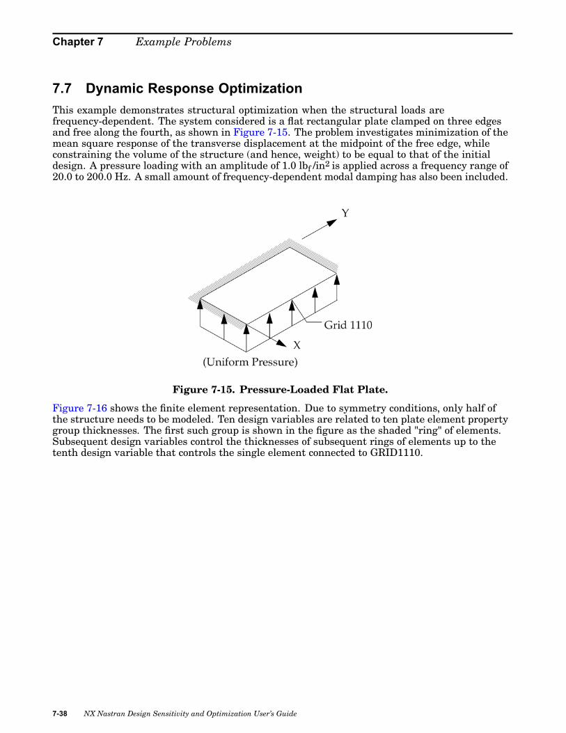
Chapter 7 Example Problems
7.7 Dynamic Response OptimizationThis example demonstrates structural optimization when the structural loads arefrequency-dependent. The system considered is a flat rectangular plate clamped on three edgesand free along the fourth, as shown in Figure 7-15. The problem investigates minimization of themean square response of the transverse displacement at the midpoint of the free edge, whileconstraining the volume of the structure (and hence, weight) to be equal to that of the initialdesign. A pressure loading with an amplitude of 1.0 lbf /in2 is applied across a frequency range of20.0 to 200.0 Hz. A small amount of frequency-dependent modal damping has also been included.
Figure 7-15. Pressure-Loaded Flat Plate.
Figure 7-16 shows the finite element representation. Due to symmetry conditions, only half ofthe structure needs to be modeled. Ten design variables are related to ten plate element propertygroup thicknesses. The first such group is shown in the figure as the shaded "ring" of elements.Subsequent design variables control the thicknesses of subsequent rings of elements up to thetenth design variable that controls the single element connected to GRID1110.
7-38 NX Nastran Design Sensitivity and Optimization User’s Guide
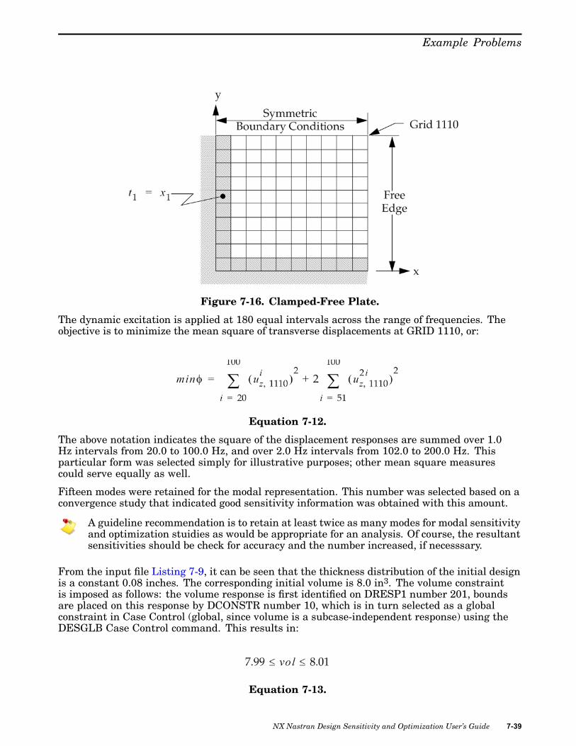
Example Problems
Figure 7-16. Clamped-Free Plate.
The dynamic excitation is applied at 180 equal intervals across the range of frequencies. Theobjective is to minimize the mean square of transverse displacements at GRID 1110, or:
Equation 7-12.
The above notation indicates the square of the displacement responses are summed over 1.0Hz intervals from 20.0 to 100.0 Hz, and over 2.0 Hz intervals from 102.0 to 200.0 Hz. Thisparticular form was selected simply for illustrative purposes; other mean square measurescould serve equally as well.
Fifteen modes were retained for the modal representation. This number was selected based on aconvergence study that indicated good sensitivity information was obtained with this amount.
A guideline recommendation is to retain at least twice as many modes for modal sensitivityand optimization stuidies as would be appropriate for an analysis. Of course, the resultantsensitivities should be check for accuracy and the number increased, if necesssary.
From the input file Listing 7-9, it can be seen that the thickness distribution of the initial designis a constant 0.08 inches. The corresponding initial volume is 8.0 in3. The volume constraintis imposed as follows: the volume response is first identified on DRESP1 number 201, boundsare placed on this response by DCONSTR number 10, which is in turn selected as a globalconstraint in Case Control (global, since volume is a subcase-independent response) using theDESGLB Case Control command. This results in:
Equation 7-13.
NX Nastran Design Sensitivity and Optimization User’s Guide 7-39

Chapter 7 Example Problems
The mean square response is to be the objective function. The underlying transversedisplacements are first identified by DRESP1 entries 20 through 100 and 102 through 200 (notethe use of Bulk Data replicators). These identify the transverse component of displacement atGRID 1110 across the frequency range of interest. These first-level responses are then used asinput to DEQATN 1 via DRESP2 number 1, which defines the equation input. The resultantresponse is then defined as the objective function using the Case Control DESOBJ command.
Optimization results are shown in Figure 7-17 and Figure 7-18. Figure 7-17 shows the designcycle history where it can be seen that the objective has been reduced from 230.13 to 133.33 in3.This took ten design cycles. (Note that CONV1, the relative measure of convergence with respectto the design objective, has been set to 0.01 on the DOPTPRM entry. This indicates convergenceas long as the objective is changing less than 1% on subsequent design cycles. Better resultswere obtained with the default, but it required twenty design cycles to achieve an objective of128.47 in2 —not that much better considering the cost involved.)
7-40 NX Nastran Design Sensitivity and Optimization User’s Guide

Example Problems
Figure 7-17. Design Cycle History
Figure 7-18. Frequency-Dependent Displacements.
Figure 7-18 shows the initial and final response data for the displacements used to formulatethe objective. Note that the integral of the final curve is indeed less than that of the originalcurve. In addition, the response peak has shifted somewhat, from a value of 3.622 at 58 Hz to avalue of 2.931 at 51 Hz., indicating a slight decrease in overall structural stiffness. Figure7-19 shows the final thickness distribution.
NX Nastran Design Sensitivity and Optimization User’s Guide 7-41

Chapter 7 Example Problems
Figure 7-19. Final Thickness Distribution.
$ Unit Test Data Deck$ d200t4af: SOL200, V68$ID EDS, D200t4afTIME 100SOL 200CENDTITLE = Synthesis of Responses across Different Frequencies: d200t4afSET 10 = 1110DISPL(PHASE,SORT1) = 10 $ MAGNITUDE/PHASE REPRESENTATION FOR RESPONSE$ ANALYSIS AS WELL AS SENSITIVITY ANALYSISdesglb = 10subcase 1SPC = 100LOADSET = 720DLOAD = 700FREQ = 740METHOD = 500ANALYSIS = MFREQsdamping = 2000DESOBJ = 1outputdisp(plot,phase) = 10
output(xyout)cscale 2.0ymax=4.0plotter = nastranytitle = displacement at grid 1110xyplot disp / 1110(t3)
$BEGIN BULKPARAM, WTMASS, .002588$-------------------------------------------------------------------------------$ ANALYSIS MODEL$-------------------------------------------------------------------------------$$...GRID AND SPC DATA:$GRDSET, , , , , , , 6GRID, 100, , 0., 0., 0.=, *(1), , *(1.), =, ==9GRID, 200, , 0., 1.0, 0.=, *(1), , *(1.), =, ==9GRID, 300, , 0., 2.0, 0.=, *(1), , *(1.), =, ==9
7-42 NX Nastran Design Sensitivity and Optimization User’s Guide

Example Problems
GRID, 400, , 0., 3.0, 0.=, *(1), , *(1.), =, ==9GRID, 500, , 0., 4.0, 0.=, *(1), , *(1.), =, ==9GRID, 600, , 0., 5.0, 0.=, *(1), , *(1.), =, ==9GRID, 700, , 0., 6.0, 0.=, *(1), , *(1.), =, ==9GRID, 800, , 0., 7.0, 0.=, *(1), , *(1.), =, ==9GRID, 900, , 0., 8.0, 0.=, *(1), , *(1.), =, ==9GRID, 1000, , 0., 9.0, 0.=, *(1), , *(1.), =, ==9GRID, 1100, , 0., 10.0, 0.=, *(1), , *(1.), =, ==9$SPC1, 100, 123456 100, 101, 102, 103, 104, 105, ++, 106, 107, 108, 109, 110, 200, 300, 400, ++, 500, 600, 700, 800, 900, 1000, 1100SPC1, 100, 246, 1101, 1102, 1103, 1104, 1105, 1106, ++, 1107, 1108, 1109SPC1, 100, 246, 1110$$...ELEMENT DEFINITION AND PROPERTIES:$ (ELEMENTS GROUPED BY PID SINCE THICKNESS OF ALL ELEMENTS IN A GROUP$ ARE TO BE AFFECTED BY A SINGLE DESIGN VARIABLE)$MAT1, 150, 1.0E7, , 0.3, 0.1$...ELEMENT GROUP 1:CQUAD4, 101, 1, 100, 101, 201, 200=, *(100), =, *(100), *(100), *(100), *(100)=8CQUAD4, 102, 1, 101, 102, 202, 201=, *(1), =, *(1), *(1), *(1), *(1),=7PSHELL, 1, 150, .08, 150$...ELEMENT GROUP 2:CQUAD4, 202, 2, 201, 202, 302, 301=, *(100), =, *(100), *(100), *(100), *(100)=7CQUAD4, 203, 2, 202, 203, 303, 302=, *(1), =, *(1), *(1), *(1), *(1),=6PSHELL, 2, 150, .08, 150$...ELEMENT GROUP 3:CQUAD4, 303, 3, 302, 303, 403, 402=, *(100), =, *(100), *(100), *(100), *(100)=6CQUAD4, 304, 3, 303, 304, 404, 403=, *(1), =, *(1), *(1), *(1), *(1),=5PSHELL, 3, 150, .08, 150$...ELEMENT GROUP 4:CQUAD4, 404, 4, 403, 404, 504, 503=, *(100), =, *(100), *(100), *(100), *(100)=5CQUAD4, 405, 4, 404, 405, 505, 504=, *(1), =, *(1), *(1), *(1), *(1),=4PSHELL, 4, 150, .08, 150$...ELEMENT GROUP 5:CQUAD4, 505, 5, 504, 505, 605, 604=, *(100), =, *(100), *(100), *(100), *(100)=4CQUAD4, 506, 5, 505, 506, 606, 605=, *(1), =, *(1), *(1), *(1), *(1),=3PSHELL, 5, 150, .08, 150$...ELEMENT GROUP 6:CQUAD4, 606, 6, 605, 606, 706, 705=, *(100), =, *(100), *(100), *(100), *(100)=3CQUAD4, 607, 6, 606, 607, 707, 706=, *(1), =, *(1), *(1), *(1), *(1),=2PSHELL, 6, 150, .08, 150$...ELEMENT GROUP 7:CQUAD4, 707, 7, 706, 707, 807, 806=, *(100), =, *(100), *(100), *(100), *(100)=2CQUAD4, 708, 7, 707, 708, 808, 807
NX Nastran Design Sensitivity and Optimization User’s Guide 7-43

Chapter 7 Example Problems
=, *(1), =, *(1), *(1), *(1), *(1),=1PSHELL, 7, 150, .08, 150$...ELEMENT GROUP 8:CQUAD4, 808, 8, 807, 808, 908, 907=, *(100), =, *(100), *(100), *(100), *(100)=1CQUAD4, 809, 8, 808, 809, 909, 908=, *(1), =, *(1), *(1), *(1), *(1),PSHELL, 8, 150, .08, 150$...ELEMENT GROUP 9:CQUAD4, 909, 9, 908, 909, 1009, 1008=, *(100), =, *(100), *(100), *(100), *(100)CQUAD4, 910, 9, 909, 910, 1010, 1009PSHELL, 9, 150, .08, 150$...ELEMENT GROUP 10:CQUAD4, 1010, 10, 1009, 1010, 1110, 1109PSHELL, 10, 150, .08, 150$$...EIGENVALUE EXTRACTION INFORMATION - 15 RETAINED MODES$EIGRL 500 15 0$$...FREQUENCY DEPENDENT LOADING DATA: (OSCILLATORY PRESSURE LOAD)$RLOAD1, 700, 710, , , 800LSEQ, 720, 710, 730PLOAD2, 730, 1.0, 101, THRU, 110PLOAD2, 730, 1.0, 201, THRU, 210PLOAD2, 730, 1.0, 301, THRU, 310PLOAD2, 730, 1.0, 401, THRU, 410PLOAD2, 730, 1.0, 501, THRU, 510PLOAD2, 730, 1.0, 601, THRU, 610PLOAD2, 730, 1.0, 701, THRU, 710PLOAD2, 730, 1.0, 801, THRU, 810PLOAD2, 730, 1.0, 901, THRU, 910PLOAD2, 730, 1.0, 1001, THRU, 1010TABLED1,800, , , , , , , , ++, 0.0, 1.0, 1.0E3, 1.0, ENDT$FREQ1 740 20. 1. 180tabdmp1 20000.0 0.20 1000.0 0.20 endt
$$-------------------------------------------------------------------------------$ DESIGN MODEL$-------------------------------------------------------------------------------$$...SPECIFY DESIGN VARIABLES, RELATE LINEARLY TO PLATE THICKNESSDESVAR, 1, T1, .08, .001, 1.0DESVAR, 2, T2, .08, .001, 1.0DESVAR, 3, T3, .08, .001, 1.0DESVAR, 4, T4, .08, .001, 1.0DESVAR, 5, T5, .08, .001, 1.0DESVAR, 6, T6, .08, .001, 1.0DESVAR, 7, T7, .08, .001, 1.0DESVAR, 8, T8, .08, .001, 1.0DESVAR, 9, T9, .08, .001, 1.0DESVAR, 10, T10, .08, .001, 1.0$$...RELATE DESIGN VARIABLES TO PLATE THICKNESSESDVPREL1,101, PSHELL, 1, 4, .01, , , , +00=, *(1), =, *(1), =, =, =, =, =, *(1)=8+00, 1, 1.0*(1), *(1), ==8$DRESP1 201 VOLUME VOLUMEDRESP1 20 g1110L FRDISP 3 20.0 1110= *(1) = = = = = *(1.0) ==79DRESP1 102 G1110H FRDISP 3 102.0 1110= *(2) = = = = = *(2.0) ==48$DRESP2 1 UZ2 1DRESP1 20 21 22 23 24 25 2627 28 29 30 31 32 3334 35 36 37 38 39 4041 42 43 44 45 46 4748 49 50 51 52 53 5455 56 57 58 59 60 6162 63 64 65 66 67 6869 70 71 72 73 74 7576 77 78 79 80 81 8283 84 85 86 87 88 8990 91 92 93 94 95 9697 98 99 100 102 104 106108 110 112 114 116 118 120
7-44 NX Nastran Design Sensitivity and Optimization User’s Guide

Example Problems
122 124 126 128 130 132 134136 138 140 142 144 146 148150 152 154 156 158 160 162164 166 168 170 172 174 176178 180 182 184 186 188 190192 194 196 198 200
$DEQATN 1 UZ2(U20,u21,u22,u23,u24,u25,U26,U27,U28,U29,U30,
U31,U32,U33,U34,U35,U36,U37,U38,U39,U40,U41,U42,U43,U44,U45,U46,U47,U48,U49,U50,U51,U52,U53,U54,U55,U56,U57,U58,U59,U60,U61,U62,U63,U64,U65,U66,U67,U68,U69,U70,U71,U72,U73,U74,U75,U76,U77,U78,U79,U80,U81,U82,U83,U84,U85,U86,U87,U88,U89,U90,U91,U92,U93,U94,U95,U96,U97,U98,U99,U100,U102,U104,U106,U108,U110,U112,U114,U116,U118,U120,U122,U124,U126,U128,U130,U132,U134,U136,U138,U140,U142,U144,U146,U148,U150,U152,U154,U156,U158,U160,U162,U164,U166,U168,U170,U172,U174,U176,U178,U180,U182,U184,U186,U188,U190,U192,U194,U196,U198,U200)
= u20**2 + u21**2 + U22**2 + U23**2+ U24**2 +U25**2 + U26**2 + U27**2 + U28**2 + U29**2 +U30**2 +U31**2 + U32**2 + U33**2 + U34**2 + U35**2 +U36**2 + U37**2 + U38**2 + U39**2 + U40**2 +U41**2 + U42**2 + U43**2 + U44**2 + U45**2 +U46**2 + U47**2 + U48**2 + U49**2 + U50**2 +U50**2 + U52**2 + U53**2 + U54**2 + U55**2 +u56**2 + u57**2 + u58**2 + u59**2 + u60**2 +U61**2 + U62**2 + U63**2 + U64**2 + U65**2 +U66**2 + U67**2 + U68**2 + U69**2 + U70**2 +U71**2 + U72**2 + U73**2 + U74**2 + U75**2 +U76**2 + U77**2 + U78**2 + U79**2 + U80**2 +U80**2 + U82**2 + U83**2 + U84**2 + U85**2 +u86**2 + u87**2 + u88**2 + u89**2 + u90**2 +U90**2 + U92**2 + U93**2 + U94**2 + U95**2 +u96**2 + u97**2 + u98**2 + u99**2 + u100**2 +2.0*(u102**2 + u104**2 + u106**2 + u108**2 + u110**2 +u112**2 + u114**2 + u116**2 + u118**2 + u120**2 +u122**2 + u124**2 + u126**2 + u128**2 + u130**2 +u132**2 + u134**2 + u136**2 + u138**2 + u140**2 +u142**2 + u144**2 + u146**2 + u148**2 + u150**2 +u152**2 + u154**2 + u156**2 + u158**2 + u160**2 +u162**2 + u164**2 + u166**2 + u168**2 + u170**2 +u172**2 + u174**2 + u176**2 + u178**2 + u180**2 +u182**2 + u184**2 + u186**2 + u188**2 + u190**2 +u192**2 + u194**2 + u196**2 + u198**2 + u200**2)
$DCONSTR 10 201 7.99 8.01doptprm desmax 40 p1 1 p2 8 conv1 0.01$.......2.......3.......4.......5.......6.......7.......8.......9.......0$$param, optexit, 2ENDDATA
Listing 7-8.
7.8 Twenty-Five Bar Truss, Superelement OptimizationThis problem, often seen in the design optimization literature, calls for a minimum weightstructure subject to member stress, Euler buckling, and joint displacement constraints. Thestructure is shown in Figure 7-20. The formulation of the buckling constraints is a good exampleof constructing normalized constraints based on user-defined structural responses.
In addition, this problem will be substructured in order to illustrate superelement optimization.
NX Nastran Design Sensitivity and Optimization User’s Guide 7-45

Chapter 7 Example Problems
Figure 7-20. Twenty-Five Bar Truss.
Analysis Model Description
Three-dimensional truss tower
Symmetric with respect to x-y plane and y-z plane
Weight density = 0.1 lbs/in3
Materials: E = 1.0E7 psi
Two distinct loading conditions
Design Model Description
Minimization of structural weight
Design variables: Cross-sectional areas linked to eight independent design variables
Constraints: Allowable stress: Tensile = 40,000 psi Compressive = -40,000 psi
Displacement constraints: +0.35 inches at grid 1 and 2 for alltranslational degrees of freedom
Euler buckling constraints for compressive members assuming tubularsection diameter to thickness ratio of approximately 100
Euler buckling occurs when the magnitude of a member’s compressive stress is greater than acritical stress that, for the first buckling mode of a pin-connected member, is
7-46 NX Nastran Design Sensitivity and Optimization User’s Guide

Example Problems
Equation 7-14.
We will assume thin-walled tubular members with a diameter-to-thickness ratio of approximately100. Under this condition, the cross-sectional area A is nearly equal to
Equation 7-15.
and the area moment of inertia can be approximated by
Equation 7-16.
Since cross-sectional areas are chosen as design variables, we seek to express the memberbuckling stresses as functions of member areas as follows:
Equation 7-17.
for the buckling stress constraints to be satisfied, the member stresses must not be morecompressive than σb , that is,
Equation 7-18.
where is a negative quantity, representing a compressive stress.
Since the constraint in the form of Eq. 7-18 can’t be used directly on a DCONSTR entry (thebound is a function of the design variables), we can first normalize the expression as
Equation 7-19.
This is now a well-posed constraint, since the feasible condition has now been normalized to beon the order of 1.0. Since the lower bound is not of interest (e.g. tensile stresses on the elements
NX Nastran Design Sensitivity and Optimization User’s Guide 7-47

Chapter 7 Example Problems
will not induce Euler buckling), we can just set it to a large negative number on the DCONSTRentry, say -1.0E-10.
Eight independent design variables (DESVAR 1 through 8) are used to describe eight RODcross-sectional areas on DVPREL1 entries 1 through 8. Axial stresses and grid displacementsare identified on DRESP1 entries 1 through 14 and are constrained using DCONSTR entrieswith an I.D. of 10. Additionally, the axial rod stresses are used as input in the definition of theEuler buckling responses (DRESP2s 16 through 23), which all reference DEQATN 1. Notethat element lengths are included in these relations via constants defined on the DTABLEentry. This simplifies the input since the element lengths do not need to be hard-coded on eightdifferent DEQATN entries.
Turning to the superelement analysis model, in Case Control the SUPER = ALL command isrecommended, rather than an explicit data recovery subcase for each superelement. In BulkData, the SESET has been used to place grids 1 and 2 on the interior of superelement 1.
As far as the superelement aspects of the design model are concerned, the only necessaryaddition is in field 9 are of the DRESP1 number 15 entry. Here, "ALL" has been used to indicatethe total structural weight across all superelements be computed and used as the objectiveFunction. The default zero value for this field would have computed the weight using just thoseelements in the residual structure.
Note that the initial design is infeasible as indicated by the maximum constraint value in thesummary of design cycle history. After eight design cycles and a total of nine finite elementanalyses, a lighter weight structure is found that satisfies all constraints.
***** NORMAL CONVERGENCE CRITERIA SATISFIED ***** (HARD CONVERGENCE DECISION LOGIC)**************************************************************************************
CONVERGENCE ACHIEVED BASED ON THE FOLLOWING CRITERIA(HARD CONVERGENCE DECISION LOGIC)
RELATIVE CHANGE IN OBJECTIVE 5.2768E-05 MUST BE LESS THAN 1.0000E-03OR ABSOLUTE CHANGE IN OBJECTIVE 2.8809E-02 MUST BE LESS THAN 1.0000E-02
--- AND ---MAXIMUM CONSTRAINT VALUE 3.8660E-04 MUST BE LESS THAN 5.0000E-03
(CONVERGENCE TO A FEASIBLE DESIGN)--- OR ---
MAXIMUM OF RELATIVE PROP. CHANGES 3.8638E-02 MUST BE LESS THAN 1.0000E-03AND MAXIMUM OF RELATIVE D.V. CHANGES 3.8638E-02 MUST BE LESS THAN 1.0000E-03
(CONVERGENCE TO A BEST COMPROMISE INFEASIBLE DESIGN)**************************************************************************************
***************************************************************S U M M A R Y O F D E S I G N C Y C L E H I S T O R Y***************************************************************
(HARD CONVERGENCE ACHIEVED)NUMBER OF FINITE ELEMENT ANALYSES COMPLETED 9NUMBER OF OPTIMIZATIONS W.R.T. APPROXIMATE MODELS 8
OBJECTIVE AND MAXIMUM CONSTRAINT HISTORY---------------------------------------------------------------------------------------------------------------
OBJECTIVE FROM OBJECTIVE FROM FRACTIONAL ERROR MAXIMUM VALUECYCLE APPROXIMATE EXACT OF OFNUMBER OPTIMIZATION ANALYSIS APPROXIMATION CONSTRAINT
---------------------------------------------------------------------------------------------------------------INITIAL 6.614414E+02 1.102773E-01
1 5.985143E+02 5.985219E+02 -1.254311E-05 2.294609E-032 5.763787E+02 5.763831E+02 -7.730217E-06 8.119856E-043 5.605763E+02 5.605792E+02 -5.117301E-06 3.697191E-044 5.513699E+02 5.513676E+02 4.206515E-06 2.951452E-035 5.484974E+02 5.484994E+02 -3.560852E-06 3.337860E-056 5.465300E+02 5.465295E+02 7.817438E-07 1.285757E-047 5.459542E+02 5.459532E+02 1.788729E-06 3.235681E-068 5.459244E+02 5.459244E+02 0.000000E+00 3.865957E-04
---------------------------------------------------------------------------------------------------------------
7-48 NX Nastran Design Sensitivity and Optimization User’s Guide

Example Problems
DESIGN VARIABLE HISTORY--------------------------------------------------------------------------------------------------------------------------------
INTERNAL | EXTERNAL | |DV. ID. | DV. ID. | LABEL | INITIAL : 1 : 2 : 3 : 4 : 5 :
--------------------------------------------------------------------------------------------------------------------------------1 | 1 | X1 | 2.0000E+00 : 1.0000E+00 : 9.3000E-01 : 4.6500E-01 : 2.3250E-01 : 1.1625E-01 :2 | 2 | X2 | 2.0000E+00 : 2.0461E+00 : 2.0175E+00 : 2.0560E+00 : 2.0416E+00 : 2.0378E+00 :3 | 3 | X3 | 2.0000E+00 : 3.0000E+00 : 3.1355E+00 : 3.0361E+00 : 3.0550E+00 : 3.0211E+00 :4 | 4 | X4 | 2.0000E+00 : 1.0000E+00 : 8.6000E-01 : 4.3000E-01 : 2.1500E-01 : 1.0750E-01 :5 | 5 | X5 | 2.0000E+00 : 1.0000E+00 : 8.6240E-01 : 4.3120E-01 : 2.1558E-01 : 1.0774E-01 :6 | 6 | X6 | 2.0000E+00 : 1.0000E+00 : 6.1363E-01 : 7.1806E-01 : 6.8686E-01 : 6.6251E-01 :7 | 7 | X7 | 2.0000E+00 : 1.5944E+00 : 1.5890E+00 : 1.5927E+00 : 1.5991E+00 : 1.6201E+00 :8 | 8 | X8 | 2.0000E+00 : 2.5863E+00 : 2.7106E+00 : 2.6171E+00 : 2.6308E+00 : 2.6893E+00 :
--------------------------------------------------------------------------------------------------------------------------------INTERNAL | EXTERNAL | |DV. ID. | DV. ID. | LABEL | 6 : 7 : 8 : 9 : 10 : 11 :
--------------------------------------------------------------------------------------------------------------------------------1 | 1 | X1 | 5.8125E-02 : 2.9063E-02 : 2.8529E-02 :2 | 2 | X2 | 2.0443E+00 : 2.0427E+00 : 2.0427E+00 :3 | 3 | X3 | 3.0237E+00 : 3.0059E+00 : 3.0061E+00 :4 | 4 | X4 | 5.3750E-02 : 2.6875E-02 : 2.5837E-02 :5 | 5 | X5 | 5.3789E-02 : 5.4376E-02 : 5.3374E-02 :6 | 6 | X6 | 6.8365E-01 : 6.8306E-01 : 6.8303E-01 :7 | 7 | X7 | 1.6118E+00 : 1.6216E+00 : 1.6215E+00 :8 | 8 | X8 | 2.6649E+00 : 2.6690E+00 : 2.6691E+00 :
--------------------------------------------------------------------------------------------------------------------------------*** USER INFORMATION MESSAGE 6464 (DOM12E)
RUN TERMINATED DUE TO HARD CONVERGENCE TO AN OPTIMUM AT CYCLE NUMBER = 8.
ID UGS, D200X3TIME 10SOL 200 $ OPTIMIZATIONCENDsuper = allECHO = UNSORTOLOAD = ALLDISP = ALLSPCFORCE = ALLELFORCE = ALLSTRESS = ALLSPC = 100ANALYSIS = STATICS $DESOBJ(MIN) = 15 $ OBJECTIVE FUNCTION DEFINITIONDESSUB = 12 $ CONSTRAINT DEFININITIONSUBCASE 1
LABEL = LOAD CONDITION 1LOAD = 300
SUBCASE 2LABEL = LOAD CONDITION 2LOAD = 310
BEGIN BULK$$-------------------------------------------------------------------------------$ ANALYSIS MODEL$-------------------------------------------------------------------------------$GRDSET, , , , , , , 456SESET, 1, 1, 2MAT1, 1, 10.0E6, , , 0.1, , , , +M1+M1, 25000., 25000.SPC1, 100, 123, 7, THRU, 10GRID, 1 , , -37.5, 0.0, 200.0GRID, 2 , , 37.5, 0.0, 200.0GRID, 3 , , -37.5, 37.5, 100.0GRID, 4 , , 37.5, 37.5, 100.0GRID, 5 , , 37.5, -37.5, 100.0GRID, 6 , , -37.5, -37.5, 100.0GRID, 7 , , -100.0, 100.0, 0.0GRID, 8 , , 100.0, 100.0, 0.0GRID, 9 , , 100.0, -100.0, 0.0GRID, 10, , -100.0, -100.0, 0.0CROD, 1 , 1, 1, 2CROD, 2 , 2, 1, 4CROD, 3 , 2, 2, 3CROD, 4 , 2, 1, 5CROD, 5 , 2, 2, 6CROD, 6 , 3, 2, 4CROD, 7 , 3, 2, 5CROD, 8 , 3, 1, 3CROD, 9 , 3, 1, 6CROD, 10, 4, 3, 6CROD, 11, 4, 4, 5CROD, 12, 5, 3, 4CROD, 13, 5, 5, 6CROD, 14, 6, 3, 10CROD, 15, 6, 6, 7CROD, 16, 6, 4, 9CROD, 17, 6, 5, 8CROD, 18, 7, 4, 7CROD, 19, 7, 3, 8
NX Nastran Design Sensitivity and Optimization User’s Guide 7-49
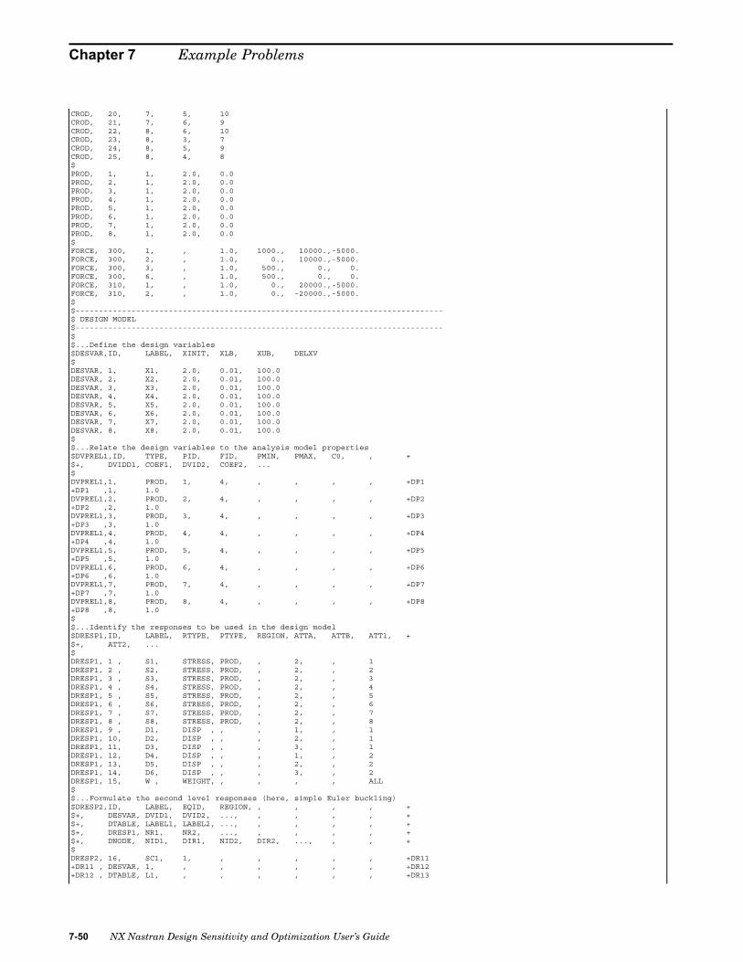
Chapter 7 Example Problems
CROD, 20, 7, 5, 10CROD, 21, 7, 6, 9CROD, 22, 8, 6, 10CROD, 23, 8, 3, 7CROD, 24, 8, 5, 9CROD, 25, 8, 4, 8$PROD, 1, 1, 2.0, 0.0PROD, 2, 1, 2.0, 0.0PROD, 3, 1, 2.0, 0.0PROD, 4, 1, 2.0, 0.0PROD, 5, 1, 2.0, 0.0PROD, 6, 1, 2.0, 0.0PROD, 7, 1, 2.0, 0.0PROD, 8, 1, 2.0, 0.0$FORCE, 300, 1, , 1.0, 1000., 10000.,-5000.FORCE, 300, 2, , 1.0, 0., 10000.,-5000.FORCE, 300, 3, , 1.0, 500., 0., 0.FORCE, 300, 6, , 1.0, 500., 0., 0.FORCE, 310, 1, , 1.0, 0., 20000.,-5000.FORCE, 310, 2, , 1.0, 0., -20000.,-5000.$$-------------------------------------------------------------------------------$ DESIGN MODEL$-------------------------------------------------------------------------------$$...Define the design variables$DESVAR,ID, LABEL, XINIT, XLB, XUB, DELXV$DESVAR, 1, X1, 2.0, 0.01, 100.0DESVAR, 2, X2, 2.0, 0.01, 100.0DESVAR, 3, X3, 2.0, 0.01, 100.0DESVAR, 4, X4, 2.0, 0.01, 100.0DESVAR, 5, X5, 2.0, 0.01, 100.0DESVAR, 6, X6, 2.0, 0.01, 100.0DESVAR, 7, X7, 2.0, 0.01, 100.0DESVAR, 8, X8, 2.0, 0.01, 100.0$$...Relate the design variables to the analysis model properties$DVPREL1,ID, TYPE, PID, FID, PMIN, PMAX, C0, , +$+, DVIDD1, COEF1, DVID2, COEF2, ...$DVPREL1,1, PROD, 1, 4, , , , , +DP1+DP1 ,1, 1.0DVPREL1,2, PROD, 2, 4, , , , , +DP2+DP2 ,2, 1.0DVPREL1,3, PROD, 3, 4, , , , , +DP3+DP3 ,3, 1.0DVPREL1,4, PROD, 4, 4, , , , , +DP4+DP4 ,4, 1.0DVPREL1,5, PROD, 5, 4, , , , , +DP5+DP5 ,5, 1.0DVPREL1,6, PROD, 6, 4, , , , , +DP6+DP6 ,6, 1.0DVPREL1,7, PROD, 7, 4, , , , , +DP7+DP7 ,7, 1.0DVPREL1,8, PROD, 8, 4, , , , , +DP8+DP8 ,8, 1.0$$...Identify the responses to be used in the design model$DRESP1,ID, LABEL, RTYPE, PTYPE, REGION, ATTA, ATTB, ATT1, +$+, ATT2, ...$DRESP1, 1 , S1, STRESS, PROD, , 2, , 1DRESP1, 2 , S2, STRESS, PROD, , 2, , 2DRESP1, 3 , S3, STRESS, PROD, , 2, , 3DRESP1, 4 , S4, STRESS, PROD, , 2, , 4DRESP1, 5 , S5, STRESS, PROD, , 2, , 5DRESP1, 6 , S6, STRESS, PROD, , 2, , 6DRESP1, 7 , S7, STRESS, PROD, , 2, , 7DRESP1, 8 , S8, STRESS, PROD, , 2, , 8DRESP1, 9 , D1, DISP , , , 1, , 1DRESP1, 10, D2, DISP , , , 2, , 1DRESP1, 11, D3, DISP , , , 3, , 1DRESP1, 12, D4, DISP , , , 1, , 2DRESP1, 13, D5, DISP , , , 2, , 2DRESP1, 14, D6, DISP , , , 3, , 2DRESP1, 15, W , WEIGHT, , , , , ALL$$...Formulate the second level responses (here, simple Euler buckling)$DRESP2,ID, LABEL, EQID, REGION, , , , , +$+, DESVAR, DVID1, DVID2, ..., , , , , +$+, DTABLE, LABEL1, LABEL2, ..., , , , , +$+, DRESP1, NR1, NR2, ..., , , , , +$+, DNODE, NID1, DIR1, NID2, DIR2, ..., , , +$DRESP2, 16, SC1, 1, , , , , , +DR11+DR11 , DESVAR, 1, , , , , , , +DR12+DR12 , DTABLE, L1, , , , , , , +DR13
7-50 NX Nastran Design Sensitivity and Optimization User’s Guide
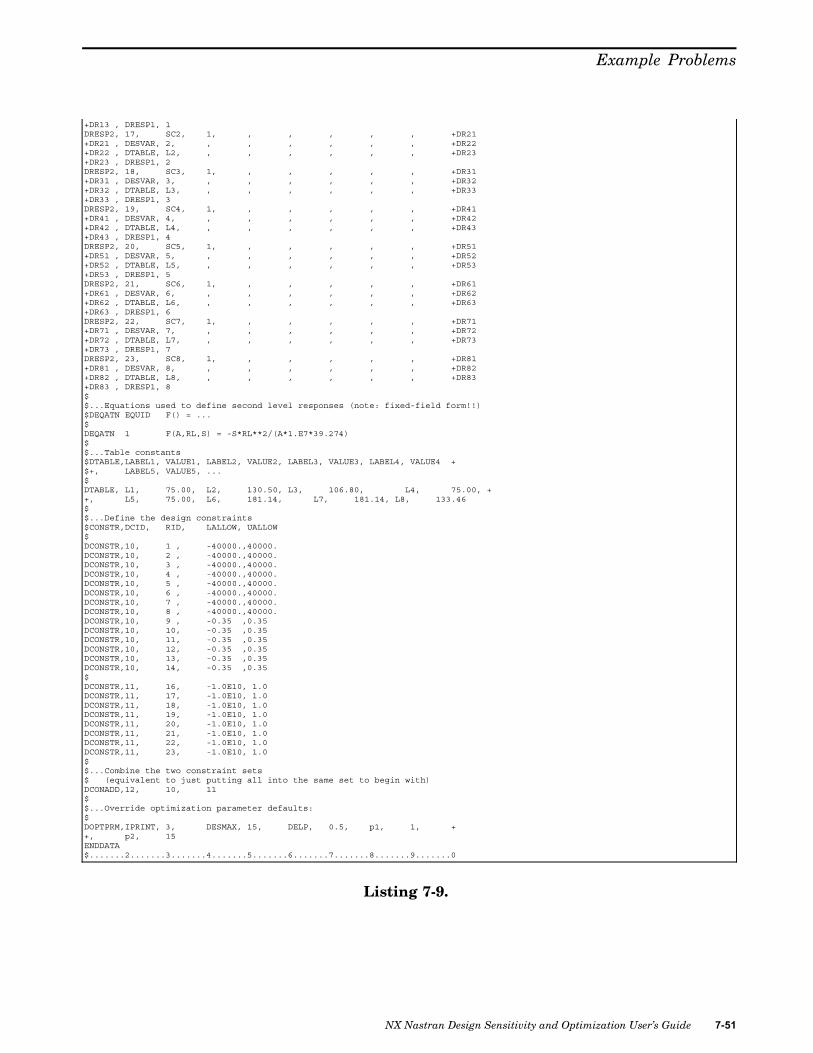
Example Problems
+DR13 , DRESP1, 1DRESP2, 17, SC2, 1, , , , , , +DR21+DR21 , DESVAR, 2, , , , , , , +DR22+DR22 , DTABLE, L2, , , , , , , +DR23+DR23 , DRESP1, 2DRESP2, 18, SC3, 1, , , , , , +DR31+DR31 , DESVAR, 3, , , , , , , +DR32+DR32 , DTABLE, L3, , , , , , , +DR33+DR33 , DRESP1, 3DRESP2, 19, SC4, 1, , , , , , +DR41+DR41 , DESVAR, 4, , , , , , , +DR42+DR42 , DTABLE, L4, , , , , , , +DR43+DR43 , DRESP1, 4DRESP2, 20, SC5, 1, , , , , , +DR51+DR51 , DESVAR, 5, , , , , , , +DR52+DR52 , DTABLE, L5, , , , , , , +DR53+DR53 , DRESP1, 5DRESP2, 21, SC6, 1, , , , , , +DR61+DR61 , DESVAR, 6, , , , , , , +DR62+DR62 , DTABLE, L6, , , , , , , +DR63+DR63 , DRESP1, 6DRESP2, 22, SC7, 1, , , , , , +DR71+DR71 , DESVAR, 7, , , , , , , +DR72+DR72 , DTABLE, L7, , , , , , , +DR73+DR73 , DRESP1, 7DRESP2, 23, SC8, 1, , , , , , +DR81+DR81 , DESVAR, 8, , , , , , , +DR82+DR82 , DTABLE, L8, , , , , , , +DR83+DR83 , DRESP1, 8$$...Equations used to define second level responses (note: fixed-field form!!)$DEQATN EQUID F() = ...$DEQATN 1 F(A,RL,S) = -S*RL**2/(A*1.E7*39.274)$$...Table constants$DTABLE,LABEL1, VALUE1, LABEL2, VALUE2, LABEL3, VALUE3, LABEL4, VALUE4 +$+, LABEL5, VALUE5, ...$DTABLE, L1, 75.00, L2, 130.50, L3, 106.80, L4, 75.00, ++, L5, 75.00, L6, 181.14, L7, 181.14, L8, 133.46$$...Define the design constraints$CONSTR,DCID, RID, LALLOW, UALLOW$DCONSTR,10, 1 , -40000.,40000.DCONSTR,10, 2 , -40000.,40000.DCONSTR,10, 3 , -40000.,40000.DCONSTR,10, 4 , -40000.,40000.DCONSTR,10, 5 , -40000.,40000.DCONSTR,10, 6 , -40000.,40000.DCONSTR,10, 7 , -40000.,40000.DCONSTR,10, 8 , -40000.,40000.DCONSTR,10, 9 , -0.35 ,0.35DCONSTR,10, 10, -0.35 ,0.35DCONSTR,10, 11, -0.35 ,0.35DCONSTR,10, 12, -0.35 ,0.35DCONSTR,10, 13, -0.35 ,0.35DCONSTR,10, 14, -0.35 ,0.35$DCONSTR,11, 16, -1.0E10, 1.0DCONSTR,11, 17, -1.0E10, 1.0DCONSTR,11, 18, -1.0E10, 1.0DCONSTR,11, 19, -1.0E10, 1.0DCONSTR,11, 20, -1.0E10, 1.0DCONSTR,11, 21, -1.0E10, 1.0DCONSTR,11, 22, -1.0E10, 1.0DCONSTR,11, 23, -1.0E10, 1.0$$...Combine the two constraint sets$ (equivalent to just putting all into the same set to begin with)DCONADD,12, 10, 11$$...Override optimization parameter defaults:$DOPTPRM,IPRINT, 3, DESMAX, 15, DELP, 0.5, p1, 1, ++, p2, 15ENDDATA$.......2.......3.......4.......5.......6.......7.......8.......9.......0
Listing 7-9.
NX Nastran Design Sensitivity and Optimization User’s Guide 7-51
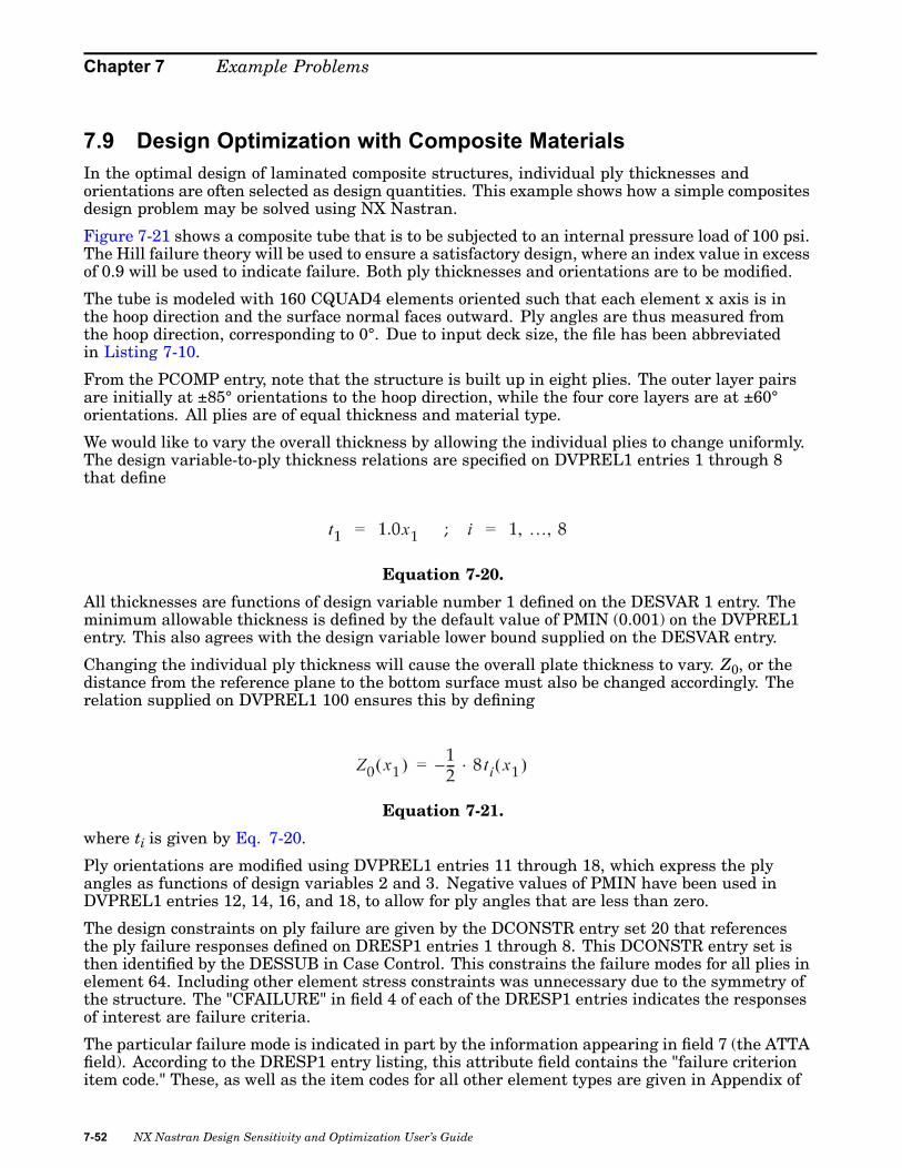
Chapter 7 Example Problems
7.9 Design Optimization with Composite MaterialsIn the optimal design of laminated composite structures, individual ply thicknesses andorientations are often selected as design quantities. This example shows how a simple compositesdesign problem may be solved using NX Nastran.
Figure 7-21 shows a composite tube that is to be subjected to an internal pressure load of 100 psi.The Hill failure theory will be used to ensure a satisfactory design, where an index value in excessof 0.9 will be used to indicate failure. Both ply thicknesses and orientations are to be modified.
The tube is modeled with 160 CQUAD4 elements oriented such that each element x axis is inthe hoop direction and the surface normal faces outward. Ply angles are thus measured fromthe hoop direction, corresponding to 0°. Due to input deck size, the file has been abbreviatedin Listing 7-10.
From the PCOMP entry, note that the structure is built up in eight plies. The outer layer pairsare initially at ±85° orientations to the hoop direction, while the four core layers are at ±60°orientations. All plies are of equal thickness and material type.
We would like to vary the overall thickness by allowing the individual plies to change uniformly.The design variable-to-ply thickness relations are specified on DVPREL1 entries 1 through 8that define
Equation 7-20.
All thicknesses are functions of design variable number 1 defined on the DESVAR 1 entry. Theminimum allowable thickness is defined by the default value of PMIN (0.001) on the DVPREL1entry. This also agrees with the design variable lower bound supplied on the DESVAR entry.
Changing the individual ply thickness will cause the overall plate thickness to vary. Z0, or thedistance from the reference plane to the bottom surface must also be changed accordingly. Therelation supplied on DVPREL1 100 ensures this by defining
Equation 7-21.
where ti is given by Eq. 7-20.
Ply orientations are modified using DVPREL1 entries 11 through 18, which express the plyangles as functions of design variables 2 and 3. Negative values of PMIN have been used inDVPREL1 entries 12, 14, 16, and 18, to allow for ply angles that are less than zero.
The design constraints on ply failure are given by the DCONSTR entry set 20 that referencesthe ply failure responses defined on DRESP1 entries 1 through 8. This DCONSTR entry set isthen identified by the DESSUB in Case Control. This constrains the failure modes for all plies inelement 64. Including other element stress constraints was unnecessary due to the symmetry ofthe structure. The "CFAILURE" in field 4 of each of the DRESP1 entries indicates the responsesof interest are failure criteria.
The particular failure mode is indicated in part by the information appearing in field 7 (the ATTAfield). According to the DRESP1 entry listing, this attribute field contains the "failure criterionitem code." These, as well as the item codes for all other element types are given in Appendix of
7-52 NX Nastran Design Sensitivity and Optimization User’s Guide

Example Problems
the NX Nastran Quick Reference Guide. Consulting this section for the CQUAD4 element showsthat the only applicable choices are 5 for ply failure or 7 for bonding material failure. The plyfailure index is determined based on the computed lamina stresses and/or strains, and theparticular failure theory selected on the PCOMP entry. With HILL selected on PCOMP 1, the 5in field 7 of each DRESP1 entry identifies Hill failure indices for use in the Design Model.
Hard convergence was achieved after thirteen design cycles as seen in Figure 7-22 andFigure 7-23. The results indicate that use of minimum allowable ply thicknesses is feasible ifcorresponding changes in ply orientation are made. The resulting orientations are and for theouter and inner plies, respectively.
Figure 7-21. Composite Tube.
Figure 7-22. Hard Convergence Output for the Composite Tube.
NX Nastran Design Sensitivity and Optimization User’s Guide 7-53

Chapter 7 Example Problems
Figure 7-23. Design History for the Composite Tube.
7-54 NX Nastran Design Sensitivity and Optimization User’s Guide

Example Problems
ID COMPOSITE,TUBESOL 200TIME 200CEND$ ANALYSIS CASE CONTROL:TITLE = TUBE UNDER INTERNAL PRESSURE - DIRECT APPROXIMATIONSUBTITLE = ANTI SYMMETRIC ANGLE-PLY [85/-85/60/-60/60/-60/85/-85]SPC = 1LOAD = 1SET 1 = 32,64STRESS = 1FORCE = 1$ OPTIMIZATION CASE CONTROL:ANALYSIS = STATICSDESOBJ(MIN) = 10DESSUB = 20BEGIN BULK$GRID 1 0 -4. 0.0 0.0GRID 2 0 -3.71915-1.472380.0GRID 3 0 -2.82843-2.828430.0
. . . . . .
. . . . . .
. . . . . .GRID 217 0 -1.472383.71915 20.GRID 218 0 -2.828432.82843 20.GRID 219 0 -3.719151.47238 20.$$CQUAD4 1 1 1 2 7 6CQUAD4 2 1 2 3 8 7CQUAD4 3 1 3 4 9 8
. . . . . . .
. . . . . . .
. . . . . . .CQUAD4 158 1 212 213 218 217CQUAD4 159 1 213 214 219 218CQUAD4 160 1 214 46 51 219$$ LAMINATE DEFINITION - ANTISYMMETRIC ANGLE PLY$ ALL PLIES ARE OF THE SAME MATERIAL KFRP (KEV 49 EPOXY)$ AND THICKNESS$$ PID ZO NSM SB FT TREF GE LAMPCOMP 1 1.3E4 HILL +PC1$ MID1 T1 THETA1 SOUT1 MID2 T2 THETA2 SOUT2+PC1 100 0.01 85.0 YES -85.0 YES +PC2+PC2 60.0 YES -60.0 YES +PC3+PC3 60.0 YES -60.0 YES +PC4+PC4 85.0 YES -85.0 YES$$ PLY MATERIAL DATA$$ ALL ALLOWABLES MUST BE DEFINED AS POSITIVE$ MID E1 E2 NU12 G12 G1Z G2Z RHOMAT8 100 1.0701E75.4375E50.4 2.523E52.523E52.523E5 0.04 +M1$ A1 A2 TREF XT XC YT YC S+M1 2.426E5 3.3205E43.0305E31.9864E41.2025E4$ GE F12 STRN$$ THIS SECTION CONTAINS THE LOADS,CONSTRAINTS, AND CONTROL BULK DATA ENTRIES$$$PLOAD4 1 1 100. ++ 0PLOAD4 1 2 100. ++ 0PLOAD4 1 3 100. ++ 0
. . . . .
. . . . .
. . . . .PLOAD4 1 158 100. ++ 0PLOAD4 1 159 100. ++ 0PLOAD4 1 160 100. ++ 0$SPC 1 1 123456 0.0SPC 1 2 123456 0.0SPC 1 3 123456 0.0SPC 1 4 123456 0.0SPC 1 5 123456 0.0SPC 1 57 123456 0.0SPC 1 58 123456 0.0SPC 1 59 123456 0.0SPC 1 60 123456 0.0SPC 1 112 123456 0.0SPC 1 113 123456 0.0SPC 1 114 123456 0.0SPC 1 115 123456 0.0
NX Nastran Design Sensitivity and Optimization User’s Guide 7-55

Chapter 7 Example Problems
SPC 1 167 123456 0.0SPC 1 168 123456 0.0SPC 1 169 123456 0.0$PARAM AUTOSPC YES$$ DESIGN MODEL$$ESVAR, ID, LABEL, XINIT, XLB, XUB, DELXVDESVAR 1 TPLY 1.0 0.001 10.0DESVAR 2 THETA 85.0 -90.0 90.0DESVAR 3 THETA 60.0 -90.0 90.0$$ DV1 - PLY THICKNESS$VPREL1,ID, TYPE, PID, FID, PMIN, PMAX, C0, , +$+, DVID1, COEF1, DVID2, COEF2, ...DVPREL1 1 PCOMP 1 13 +DV1+DV1 1 0.01DVPREL1 2 PCOMP 1 17 +DV2+DV2 1 0.01DVPREL1 3 PCOMP 1 23 +DV3+DV3 1 0.01DVPREL1 4 PCOMP 1 27 +DV4+DV4 1 0.01DVPREL1 5 PCOMP 1 33 +DV5+DV5 1 0.01DVPREL1 6 PCOMP 1 37 +DV6+DV6 1 0.01DVPREL1 7 PCOMP 1 43 +DV7+DV7 1 0.01DVPREL1 8 PCOMP 1 47 +DV8+DV8 1 0.01$$ DV 2 THETA 85/-85$ DV 3 THETA 60/-60$$VPREL1,ID, TYPE, PID, FID, PMIN, PMAX, C0, , +$+, DVID1, COEF1, DVID2, COEF2, ...DVPREL1 11 PCOMP 1 14 +DT1+DT1 2 1.0DVPREL1 12 PCOMP 1 18 -90.0 +DT2+DT2 2 -1.0DVPREL1 13 PCOMP 1 24 +DT3+DT3 3 1.0DVPREL1 14 PCOMP 1 28 -90.0 +DT4+DT4 3 -1.0DVPREL1 15 PCOMP 1 34 +DT5+DT5 3 1.0DVPREL1 16 PCOMP 1 38 -90.0 +DT6+DT6 3 -1.0DVPREL1 17 PCOMP 1 44 +DT7+DT7 2 1.0DVPREL1 18 PCOMP 1 48 -90.0 +DT8+DT8 2 -1.0$DVPREL1 100 PCOMP 1 3 -100. +DZ1+DZ1 1 -0.04$$RESP1, ID, LABEL, RTYPE, PTYPE, REGION, ATTA, ATTB, ATT1, +$+, ATT2, ...DRESP1 10 W WEIGHT$DESOBJ 10 W MINDRESP1 1 FP CFAILUREELEM 5 1 64DRESP1 2 FP CFAILUREELEM 5 2 64DRESP1 3 FP CFAILUREELEM 5 3 64DRESP1 4 FP CFAILUREELEM 5 4 64DRESP1 5 FP CFAILUREELEM 5 5 64DRESP1 6 FP CFAILUREELEM 5 6 64DRESP1 7 FP CFAILUREELEM 5 7 64DRESP1 8 FP CFAILUREELEM 5 8 64$$CONSTR,DCID, RID, LALLOW, UALLOWDCONSTR,20, 1, .001, 0.9DCONSTR,20, 2, .001, 0.9DCONSTR,20, 3, .001, 0.9DCONSTR,20, 4, .001, 0.9DCONSTR,20, 5, .001, 0.9DCONSTR,20, 6, .001, 0.9DCONSTR,20, 7, .001, 0.9DCONSTR,20, 8, .001, 0.9$DOPTPRM1
7
20
0.3DOPTPRM,IPRINT, 7, DESMAX, 20, DELP, 0.3, CONV2, 1.0E-3ENDDATA
7-56 NX Nastran Design Sensitivity and Optimization User’s Guide

Example Problems
$.......2.......3.......4.......5.......6.......7.......8.......9.......0
Listing 7-10.
7.10 Acoustic OptimizationAcoustic Optimization introduces acoustic pressures as a design response. These are computedfrom a solution of the coupled fluid-structure interaction problem. An optimal design can thus befound based not only on a consideration of acoustic pressures, but structural responses as well.
This example considers a closed box with fluid elements on the interior. An acoustic source islocated at one end of the box, with a transducer located at the opposite end. The design goal is tomodify the thicknesses of the box walls such that the peak acoustic pressure at the transducer isminimized. This is to be done without increasing the weight of the box.
The box geometry and property groups of thicknesses to be modified are shown in Figure 7-24.Six design variables are to be related to six of these property groups (the third property groupin Figure 7-24 remains fixed.) This is a relatively large model, consisting of 1000 structuralelements and 2000 fluid elements.
Figure 7-24. Acoustic Box Showing Portions Designed by Each Design Variable (Prop3 is Fixed).
An interesting feature of this, as well as many other dynamic response problems, is that anumber of response peaks may exist. In addition, during the course of design optimization thesepeaks may not only increase or decrease, but shift as well. This example presents a useful wayof addressing this problem.
Figure 7-25 shows an arbitrary pressure distribution as a function of frequency, P(f). Threefrequencies of interest are shown as f1, f2, and f3. What we would like to do is to minimize themaximum pressure response over all of these points.
Figure 7-25. Minimization of Response Peaks.
NX Nastran Design Sensitivity and Optimization User’s Guide 7-57

Chapter 7 Example Problems
We can choose a design variable to represent a peak threshold, here shown in the figure as αx (αis just a constant of proportionality to facilitate scaling the threshold). The difference betweenαx and the pressure distribution must be a positive quantity at all frequencies of interest.Thus, constraints can be written that require c1, c2, and c3 to be positive distances. The designobjective can then be to minimize αx, or
minimize
Equation 7-22.
subject to:
Equation 7-23.
As the optimizer decreases the threshold, the constraints ensure that the peaks are reduced aswell. Any number of these constraints can be written to cover all frequency ranges of interest (or,in the case of transient analysis, time steps).
Due to the size of this problem, Listing 7-12 is an excerpt of the input file consisting mainly ofthe design model entries, as well as some the analysis entries. Analysis modeling for Acoustics iscovered in the NX Nastran Reference Manual.
Turning to the listing, we see that the weight budget is established as a global constraint. Theweight response is defined on DRESP1 number 2; bounds are placed on this response withDCONSTR number 5, which is in turn referenced in Case Control by the DESGLB command.The bounds on weight allow less than one third of one percent variation from the initial weight.Allowing some variation is usually preferred over an equality constraint since it not only yields abetter conditioned problem, but is often consistent with our design goals as well.
The objective function is defined as a constant times design variable number 8 using the DRESP2number 100 entry. This refers to DEQATN 100 which defines
Equation 7-24.
This is defined as the objective function by the DESOBJ 100 Case Control command.
The constraints on response peaks are defined by first identifying the pressure responsesthemselves with DRESP1 entry number 1. This designates the "1" component of displacementat grid 11280 as the response. Since this grid is part of the fluid model, the "displacement" isactually a pressure with units of N/m2. Since the ATTB field is blank on this DRESP1 entry, theresponse is computed for all output frequencies.
These pressure responses are used as input to DEQATN 10 via DRESP2 number 11. Theseentries, in combination with DCONSTR number 10, identify constraints on pressure response ofthe form:
7-58 NX Nastran Design Sensitivity and Optimization User’s Guide

Example Problems
Equation 7-25.
Note that this is similar to Eq. 7-23, with the constant k2 added to avoid a bound of zero on theconstraint. It should be clear that the constants have been chosen to scale the objective andresponses to values that would minimize numerical difficulties and that there are really no"rules" for defining these factors.
Figure 7-26 and Figure 7-27 present the optimization results. The design cycle history of Figure7-26 shows the objective has decreased from 10000.0 to 93.475 in eleven iterations. Figure 7-27shows the magnitude of the frequency dependent pressure at the initial and final designs, and itis seen that there has been a dramatic reduction in the peak pressures from 140.5 dB to 115.0dB (from 210.7 N/m2 to 11.4 N/m2).
NX Nastran Design Sensitivity and Optimization User’s Guide 7-59

Chapter 7 Example Problems
Figure 7-26. Design Cycle History for Acoustic Optimization Example.
Figure 7-27. Acoustic Optimization Sound Pressure Levels: Initial and FinalDistributions.
Table 7-1 lists the first eight initial and final structural eigenvalues as well as the first nineinvariant fluid eigenvalues. Note that the fluid has three repeated roots at 100.4 Hz and it is thecoupling between these fluid resonances and the nearby structural resonances that creates thepeak response. It is also notable that the final design has two structural frequencies near 60Hz that are showing significant response.
7-60 NX Nastran Design Sensitivity and Optimization User’s Guide

Example Problems
Table 7-1. Structural and Fluid Eigenfrequencies in Hz.Structural Eigenfrequencie
Mode No.Initial Final
Fluid Eigenfrequencies
1 75.99 59.49 50.01
2 95.29 60.78 100.41
3 104.16 94.29 100.41
4 130.78 98.56 100.41
5 133.35 139.46 112.19
6 143.74 140.27 112.19
7 153.16 165.44 142.00
8 173.69 167.38 142.00
9 - - 142.00
ID UGSTIME 100SOL 200 $ modal frequency responseCENDSUBTITLE = acoustic and structural elementsLABEL = boxae1.dat$$ analysis case control:set 20 = 11280echo = sort(param,eigc,eigrl,freq,desvar,dconstr,dresp1,dresp2,deqatn,
dvprel1)spc = 1DISP(phase) = 20method(structure) = 20method(fluid) = 30cmethod = 10frequency = 200dload = 100partn = 20$ optimization case control:ANALYSIS = MFREQDESGLB = 5DESSUB = 10DESOBJ = 100$BEGIN BULK$EIGRL 20 200. maxeigrl ,30, 15., 155., 9, 0, , 105., maxeigc,10,clan,max,,,,,15.,300.,,,,,4$$ sound pressure levelparam,rms,yes$ reference pressure for dB and dBAparam,prefdb,2.-5$PARAM AUTOSPC no$$ fluid/structure interfaceacmodl,diff , , , ,0.01$$ structural damping:param,g,0.02$$-------2-------3-------4-------5-------6-------7-------8-------9-------10------rload1,100,101,,,102darea,101,1288,3,100.tabled1,102,0.,1.,1000.,1.,endt$freq2, 200, 1.0, 200.0, 50$-------2-------3-------4-------5-------6-------7-------8-------9-------10------freq 200 40. 50. 60. 70. 80. 90. 95.
100. 105. 110. 120. 130. 140. 150. 160.170. 180. 190. 200. 97.5 102.5
$-------2-------3-------4-------5-------6-------7-------8-------9-------10------$$$ Define the Design Variables:$$ESVAR, ID, LABEL, XINIT, XLB, XUB, DELXVDESVAR, 1, P1, 0.02493,0.0001, 1.
NX Nastran Design Sensitivity and Optimization User’s Guide 7-61

Chapter 7 Example Problems
DESVAR, 2, P2, 0.01953,0.0001, 1.DESVAR, 4, P4, 0.02047,0.0001, 1.DESVAR, 5, P5, 0.02596,0.0001, 1.DESVAR, 6, P6, 0.02175,0.0001, 1.DESVAR, 7, P7, 0.02426,0.0001, 1.DESVAR 8 BETA 1.0 0.001$$ Relate the Design Variables to changes in plate thicknesses:$$VPREL1,ID, TYPE, PID, FID, PMIN, PMAX, C0, , +$+, DVID1, COEF1, DVID2, COEF2, ...$DVPREL1,1, PSHELL, 1, 4, 0.0001, , , , ++, 1, 1.DVPREL1,2, PSHELL, 2, 4, 0.0001, , , , ++, 2, 1.DVPREL1,4, PSHELL, 4, 4, 0.0001, , , , ++, 4, 1.DVPREL1,5, PSHELL, 5, 4, 0.0001, , , , ++, 5, 1.DVPREL1,6, PSHELL, 6, 4, 0.0001, , , , ++, 6, 1.DVPREL1,7, PSHELL, 7, 4, 0.0001, , , , ++, 7, 1.$$ Define the synthetic Objective as a function of X8:$$RESP2, ID, LABEL, EQID, REGION, , , , , +$+, DESVAR, DVID1, DVID2, ..., , , , , +DRESP2 100 BETA 100DESVAR 8
DEQATN 100 OBJ(BETA) = 10000.0 * BETA$$ Define the constraint on weight (weight budget for optimization):$$RESP1, ID, LABEL, RTYPE, PTYPE, REGION, ATTA, ATTB, ATT1, +$+, ATT2, ...$DRESP1 2 WEIGHT WEIGHT$CONSTR,DCID, RID, LALLOW, UALLOWDCONSTR 5 2 2890. 2910.$$ Define the constraints on acoustic sound pressure levels$ (one for each forcing frequency):$DRESP1 1 DRUCK FRDISP 1 11280DRESP2 11 PRESBET 10DESVAR 8
DRESP1 1DEQATN 10 F(BETA,PRES) = 100.0 * BETA - PRES + 1000.DCONSTR 10 11 1000.$$ Override miscellaneous Optimization Parameters:$DOPTPRM DESMAX 20 P1 1 P2 15 CONV1 1E-6$$$$$$$$$$$$$$$$$$$$$$$$$$$$$$$$$$$$$$$$ structural model$$$$$$$$$$$$$$$$$$$$$$$$$$$$$$$$$$$$$$$$ THIS SECTION CONTAINS THE PROPERTY AND MATERIAL BULK DATA ENTRIES$PSHELL 3 1 .100 1$PSHELL 1 1 .02493 1PSHELL 2 1 .01953 1pshell 4 1 .02047 1pshell 5 1 .02596 1pshell 6 1 .02175 1pshell 7 1 .02426 1$$$ THIS SECTION CONTAINS BULK DATA FOR SUPERELEMENT 0$$GRID 1 0.0 0.0 0.0GRID 2 2. 0.0 0.0GRID 3 2. 0.0 1.
. . . . .
. . . . .
. . . . .GRID 1293 1.5 .5 1.GRID 1294 1.6 .5 1.GRID 1295 1.7 .5 1.$CQUAD4 1 1 1 9 29 28CQUAD4 2 1 9 10 30 29
. . . . . . .
. . . . . . .
7-62 NX Nastran Design Sensitivity and Optimization User’s Guide
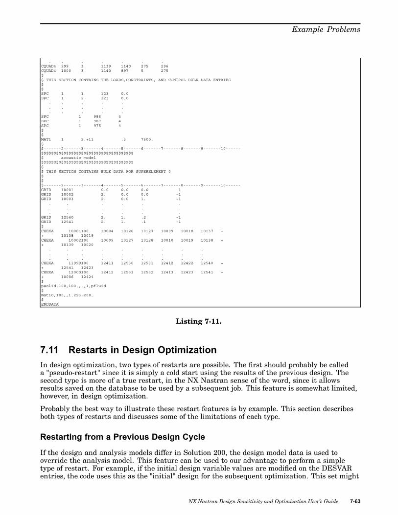
Example Problems
. . . . . . .CQUAD4 999 3 1139 1140 275 296CQUAD4 1000 3 1140 897 5 275$$ THIS SECTION CONTAINS THE LOADS,CONSTRAINTS, AND CONTROL BULK DATA ENTRIES$$SPC 1 1 123 0.0SPC 1 2 123 0.0
. . . . .
. . . . .
. . . . .SPC 1 986 4SPC 1 987 4SPC 1 975 4$$MAT1 1 2.+11 .3 7600.$$-------2-------3-------4-------5-------6-------7-------8-------9-------10------$$$$$$$$$$$$$$$$$$$$$$$$$$$$$$$$$$$$$$ acoustic model$$$$$$$$$$$$$$$$$$$$$$$$$$$$$$$$$$$$$$$ THIS SECTION CONTAINS BULK DATA FOR SUPERELEMENT 0$$$-------2-------3-------4-------5-------6-------7-------8-------9-------10------GRID 10001 0.0 0.0 0.0 -1GRID 10002 2. 0.0 0.0 -1GRID 10003 2. 0.0 1. -1
. . . . . .
. . . . . .
. . . . . .GRID 12540 2. 1. .2 -1GRID 12541 2. 1. .1 -1$CHEXA 10001100 10004 10126 10127 10009 10018 10137 ++ 10138 10019CHEXA 10002100 10009 10127 10128 10010 10019 10138 ++ 10139 10020
. . . . . . . . .
. . . . . . . . .
. . . . . . . . .CHEXA 11999100 12411 12530 12531 12412 12422 12540 ++ 12541 12423CHEXA 12000100 12412 12531 12532 12413 12423 12541 ++ 10006 12424$psolid,100,100,,,,1,pfluid$mat10,100,,1.293,200.$ENDDATA
Listing 7-11.
7.11 Restarts in Design OptimizationIn design optimization, two types of restarts are possible. The first should probably be calleda "pseudo-restart" since it is simply a cold start using the results of the previous design. Thesecond type is more of a true restart, in the NX Nastran sense of the word, since it allowsresults saved on the database to be used by a subsequent job. This feature is somewhat limited,however, in design optimization.
Probably the best way to illustrate these restart features is by example. This section describesboth types of restarts and discusses some of the limitations of each type.
Restarting from a Previous Design Cycle
If the design and analysis models differ in Solution 200, the design model data is used tooverride the analysis model. This feature can be used to our advantage to perform a simpletype of restart. For example, if the initial design variable values are modified on the DESVARentries, the code uses this as the "initial" design for the subsequent optimization. This set might
NX Nastran Design Sensitivity and Optimization User’s Guide 7-63

Chapter 7 Example Problems
have been determined based on a prior optimization cycle or may reflect other changes thatthe engineer might want to make.
For every design cycle completed, a "punch" file is created (.PCH) that contains the DESVARBulk Data entries for this latest design. The contents of the punch file can be included in theoriginal input deck to "restart" from this point in the design space.
Using the venerable Three-Bar Truss as an example (TPL deck D200X1.DAT), suppose that wewant to perform a single design cycle with some of the optimization parameters overridden,examine these results, readjust the parameters, and continue with optimization. Listing 7-12shows the input data file for the first design cycle.
The shape optimization capabilities in the software also include output of the updatedGRID entries. The parameter DESPCH controls the frequency of both updated GRIDand DESVAR entry output to the punch file. See Parameters for Design Sensitivity andOptimization .
Since displacement and stress responses vary inversely to the bar cross-sectional dimensions,APRCOD = 2 or the mixed method of approximations is selected on the DOPTPRM entry.(APRCOD = 2 is the default anyway, but this makes it explicit in the input data). Since this islikely to yield a good approximation for truss-type structures, we have increased the movelimits to 100% for this first design cycle (DELP = 1.0). With these relatively wide move limits,we may want to make sure that all of the constraints are included, just to be sure. DSCREENentries have been included to reduce the truncation threshold TRS to a large negative numberto ensure that none of the displacement or stress constraints are screened out prior to theapproximate optimization.
The design cycle history is shown in Figure 7-28. Compare these results to the original Three-BarTruss example in Three-Bar Truss. Note that the 100% move limits allow a greater move inx2 for the first cycle, which results in a somewhat lower value of the objective. (In fact, noticethat x2 actually changed by slightly more than 50% in the original problem. As mentionedin Optimization with Respect to Approximate Models , this may occur since move limits areimposed as equivalent constraints on the corresponding properties. Critical constraints may notbe satisfied exactly, as is seen to be the case here. This is usually inconsequential, since thisdesign just serves as a starting point for the next optimization cycle.)
7-64 NX Nastran Design Sensitivity and Optimization User’s Guide

Example Problems
Figure 7-28. Single Design Cycle.
Turning now to the pseudo-restart, the punch file from the previous design cycle is included inthe restart deck listed in Listing 7-13. Only the design model portion of the deck has beenincluded in Listing 7-13, since the analysis model portion is identical to Listing 7-12. Theoptimization now begins from the point in the design space defined by the new DESVAR entries.The DOPTPRM and DSCREEN entries are updated in this deck as well to allow more designiterations (DESMAX), reduce the move limits to 50% (DELP), and set the truncation thresholdback to -0.5 (TRS). (Leaving out the DSCREEN entries altogether accomplishes the same thingsince this is the TRS default.)
The optimization results from this input are listed in Figure 7-29, which are seen to be slightlybetter than the original D200X1. If this job were much larger and more complex, the abilityto pause, examine the results, and readjust some of the optimization parameters could beindispensable.
NX Nastran Design Sensitivity and Optimization User’s Guide 7-65

Chapter 7 Example Problems
Figure 7-29. Optimization from Updated Design.
Looking back on the summary of design cycle history for the first run, note that two finiteelement analyses were performed. The first provided the baseline analysis, while the secondupdated the set of responses according to the proposed design changes. The first task of thesubsequent "restart" repeats this analysis, though, to provide the new, baseline responses. If theanalysis cost is high, this repeated analysis might be troublesome. The costs associated withthis type of restart must be weighed against its convenience.
Restarting from an OPTEXIT Point
The second class of restarts is based on NX Nastran’s automatic restart capability. In designoptimization, this works in conjunction with the predefined Solution 200 exit points, OPTEXIT1 through 6. Recall that setting this parameter in Bulk Data will terminate the program atone of these six exit points.
Automatic restart for design optimization is somewhat limited since only the analysis restartlogic is in place. That is, only data associated with the analysis results are used on restart, andall design optimization-related processes are repeated. For example, restarts from an OPTEXITpoint of 4 or greater will result in a repeat of the sensitivity analysis phases. This occursregardless of whether the design model has changed or not. (Warning: the design model mustnot be changed, as unpredictable results may occur.)
To illustrate this procedure, suppose we wanted to perform a baseline analysis for the structure,compute the sensitivities of the design responses with respect to changes in the design variables,and then pause to examine these results before restarting. The results of the finite elementanalysis are saved to the database by including SCR=NO in the job submittal command.
The only difference between the original three-bar truss and the input here is the Bulk Dataparameter OPTEXIT. In this case, OPTEXIT is set to 4, which instructs the code to performsensitivity analysis, print out the coefficients, and stop.
7-66 NX Nastran Design Sensitivity and Optimization User’s Guide

Example Problems
After the finite element and sensitivity analysis results are examined and verified, the decisionis made to continue with optimization in the restart run. This deck is shown in Listing 7-14.
The RESTART command is required, and indicates that the most recent version on the databaseis to be used (VERSION=LAST), and only the latest data is to be retained (NOKEEP). If wealways intend to use the first version on the database for restarts, we can instead use,
RESTART, VERSION=1, KEEP
This command appends the subsequent results to the database while saving the data fromprior runs. This might be useful if the restart yields results that we do not want to save andwe want to go back and restart from the initial analysis. By specifying VERSION=1, KEEP, wealways have the first version to fall back on.
The command,ASSIGN MASTER=d200x1c.MASTER
assigns the correct DBSET, so we do not have to repeatedly assign this with ‘DBS = ’ in thejob submittal command. (The lower-case filename ensures consistency with the filenamingon UNIX-based machines. On some machines, quote marks may also be required around thefilename.)
‘ /,38 ’ deletes the OPTEXIT parameter assignment from the Bulk Data, which is entry number38 in the sorted data. It is usually a good idea to request a listing of the sorted Bulk Data,especially if subsequent restarts are anticipated. It is the default, anyway, but is explicit withthe Case Control command, ECHO=SORT.
The optimization results from this restart are shown in Figure 7-30. Note that they agree withthe results of the original Three-Bar Truss. The contents of the .F04 file (not included here)indicate the initial analysis was skipped.
NX Nastran Design Sensitivity and Optimization User’s Guide 7-67
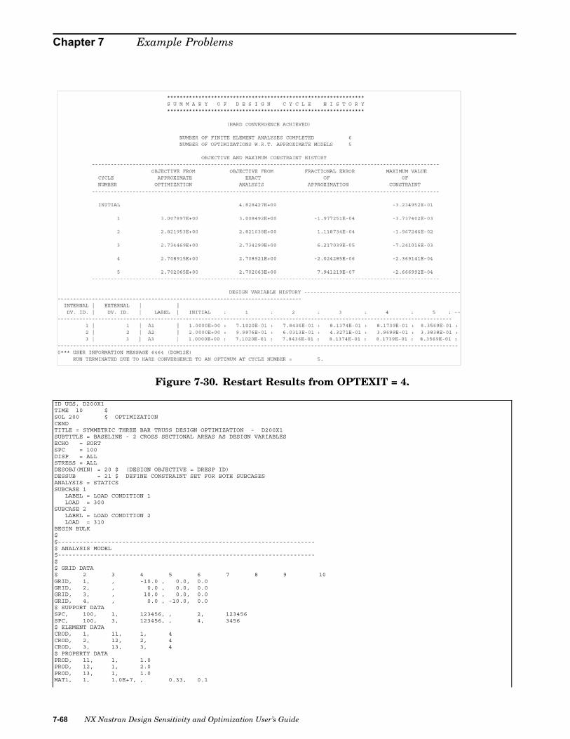
Chapter 7 Example Problems
Figure 7-30. Restart Results from OPTEXIT = 4.
ID UGS, D200X1TIME 10 $SOL 200 $ OPTIMIZATIONCENDTITLE = SYMMETRIC THREE BAR TRUSS DESIGN OPTIMIZATION - D200X1SUBTITLE = BASELINE - 2 CROSS SECTIONAL AREAS AS DESIGN VARIABLESECHO = SORTSPC = 100DISP = ALLSTRESS = ALLDESOBJ(MIN) = 20 $ (DESIGN OBJECTIVE = DRESP ID)DESSUB = 21 $ DEFINE CONSTRAINT SET FOR BOTH SUBCASESANALYSIS = STATICSSUBCASE 1
LABEL = LOAD CONDITION 1LOAD = 300
SUBCASE 2LABEL = LOAD CONDITION 2LOAD = 310
BEGIN BULK$$------------------------------------------------------------------------$ ANALYSIS MODEL$------------------------------------------------------------------------$$ GRID DATA$ 2 3 4 5 6 7 8 9 10GRID, 1, , -10.0 , 0.0, 0.0GRID, 2, , 0.0 , 0.0, 0.0GRID, 3, , 10.0 , 0.0, 0.0GRID, 4, , 0.0 , -10.0, 0.0$ SUPPORT DATASPC, 100, 1, 123456, , 2, 123456SPC, 100, 3, 123456, , 4, 3456$ ELEMENT DATACROD, 1, 11, 1, 4CROD, 2, 12, 2, 4CROD, 3, 13, 3, 4$ PROPERTY DATAPROD, 11, 1, 1.0PROD, 12, 1, 2.0PROD, 13, 1, 1.0MAT1, 1, 1.0E+7, , 0.33, 0.1
7-68 NX Nastran Design Sensitivity and Optimization User’s Guide

Example Problems
$ EXTERNAL LOADS DATAFORCE, 300, 4, , 20000., 0.8, -0.6FORCE, 310, 4, , 20000., -0.8, -0.6$$------------------------------------------------------------------------$ DESIGN MODEL$------------------------------------------------------------------------$$...DESIGN VARIABLE DEFINITION$DESVAR,ID, LABEL, XINIT, XLB, XUB, DELXV(OPTIONAL)DESVAR, 1, A1, 1.0, 0.1, 100.0DESVAR, 2, A2, 2.0, 0.1, 100.0DESVAR, 3, A3, 1.0, 0.1, 100.0$$...IMPOSE X3=X1 (LEADS TO A3=A1)$DLINK, ID, DDVID, CO, CMULT, IDV1, C1, IDV2, C2, +$+, IDV3, C3, ...DLINK, 1, 3, 0.0, 1.0, 1, 1.00$$...DEFINITION OF DESIGN VARIABLE TO ANALYSIS MODEL PARAMETER RELATIONS$DVPREL1,ID, TYPE, PID, FID, PMIN, PMAX, C0, , +$+, DVID1, COEF1, DVID2, COEF2, ...DVPREL1,10, PROD, 11, 4, , , , , +DP1+DP1, 1, 1.0DVPREL1,20, PROD, 12, 4, , , , , +DP2+DP2, 2, 1.0DVPREL1,30, PROD, 13, 4, , , , , +DP3+DP3, 3, 1.0$$...STRUCTURAL RESPONSE IDENTIFICATION$DRESP1,ID, LABEL, RTYPE, PTYPE, REGION, ATTA, ATTB, ATT1, +$+, ATT2, ...DRESP1, 20, W , WEIGHTDRESP1, 21, U4, DISP , , , 1, , 4DRESP1, 22, V4, DISP , , , 2, , 4DRESP1, 23, S1, STRESS, PROD, , 2, , 11DRESP1, 24, S2, STRESS, PROD, , 2, , 12DRESP1, 25, S3, STRESS, PROD, , 2, , 13$$...CONSTRAINTS$DCONSTR,DCID, RID, LALLOW, UALLOWDCONSTR,21, 21, -0.20 ,0.20DCONSTR,21, 22, -0.20 ,0.20DCONSTR,21, 23, -15000.,20000.DCONSTR,21, 24, -15000.,20000.DCONSTR,21, 25, -15000.,20000.$$...OPTIMIZATION CONTROL:$DSCREEN,DISP, -100., 10DSCREEN,STRESS, -100., 10DOPTPRM,APRCOD, 2, IPRINT, 5, DESMAX, 1, DELP, 1.0, ++, P1, 1, P2, 15$$.......2.......3.......4.......5.......6.......7.......8.......9.......0ENDDATA$
Listing 7-12.
$------------------------------------------------------------------------$ DESIGN MODEL$------------------------------------------------------------------------$$...DESIGN VARIABLE DEFINITION$DESVAR,ID, LABEL, XINIT, XLB, XUB, DELXV(OPTIONAL)DESVAR * 1A1 7.68653870E-01 1.00000001E-01+D 1V*D 1V 1.00000000E+02 1.00000000E+00DESVAR * 2A2 7.14803874E-01 1.00000001E-01+D 2V*D 2V 1.00000000E+02 1.00000000E+00DESVAR * 3A3 7.68653870E-01 1.00000001E-01+D 3V*D 3V 1.00000000E+02 1.00000000E+00$$...IMPOSE X3=X1 (LEADS TO A3=A1)$DLINK, ID, DDVID, CO, CMULT, IDV1, C1, IDV2, C2, +$+, IDV3, C3, ...DLINK, 1, 3, 0.0, 1.0, 1, 1.00$$...DEFINITION OF DESIGN VARIABLE TO ANALYSIS MODEL PARAMETER RELATIONS$DVPREL1,ID, TYPE, PID, FID, PMIN, PMAX, C0, , +$+, DVID1, COEF1, DVID2, COEF2, ...DVPREL1,10, PROD, 11, 4, , , , , +DP1+DP1, 1, 1.0DVPREL1,20, PROD, 12, 4, , , , , +DP2+DP2, 2, 1.0DVPREL1,30, PROD, 13, 4, , , , , +DP3+DP3, 3, 1.0$$...STRUCTURAL RESPONSE IDENTIFICATION$DRESP1,ID, LABEL, RTYPE, PTYPE, REGION, ATTA, ATTB, ATT1, +$+, ATT2, ...
NX Nastran Design Sensitivity and Optimization User’s Guide 7-69

Chapter 7 Example Problems
DRESP1, 20, W , WEIGHTDRESP1, 21, U4, DISP , , , 1, , 4DRESP1, 22, V4, DISP , , , 2, , 4DRESP1, 23, S1, STRESS, PROD, , 2, , 11DRESP1, 24, S2, STRESS, PROD, , 2, , 12DRESP1, 25, S3, STRESS, PROD, , 2, , 13$$...CONSTRAINTS$DCONSTR,DCID, RID, LALLOW, UALLOWDCONSTR,21, 21, -0.20 ,0.20DCONSTR,21, 22, -0.20 ,0.20DCONSTR,21, 23, -15000.,20000.DCONSTR,21, 24, -15000.,20000.DCONSTR,21, 25, -15000.,20000.$$...OPTIMIZATION CONTROL:$DSCREEN,DISP, -.5DSCREEN,STRESS, -.5DOPTPRM,IPRINT, 5, DESMAX, 10, DELP, 0.5, P1, 1, ++, P2, 15$$.......2.......3.......4.......5.......6.......7.......8.......9.......0ENDDATA
Listing 7-13.
RESTART, VERSION=LAST, NOKEEPASSIGN MASTER=d200x1c.MASTERID EDS, D200X1TIME 10 $SOL 200 $ OPTIMIZATIONCENDTITLE = SYMMETRIC THREE BAR TRUSS DESIGN OPTIMIZATION - D200X1SUBTITLE = BASELINE - 2 CROSS SECTIONAL AREAS AS DESIGN VARIABLESECHO = SORTSPC = 100DISP = ALLSTRESS = ALLDESOBJ(MIN) = 20 $ (DESIGN OBJECTIVE = DRESP ID)DESSUB = 21 $ DEFINE CONSTRAINT SET FOR BOTH SUBCASESANALYSIS = STATICSSUBCASE 1
LABEL = LOAD CONDITION 1LOAD = 300
SUBCASE 2LABEL = LOAD CONDITION 2LOAD = 310
BEGIN BULK/,34ENDDATA
Listing 7-14.
7-70 NX Nastran Design Sensitivity and Optimization User’s Guide

Appendix
A Glossary of Terms
Active Constraint a constraint whose numerical value is near zero. In NX Nastran, theconstant CT (default = –0.03) is used to measure whether a constraint is active or inactive. Aconstraint whose value is less than CT is deemed inactive, and if its value is greater than CT,it is considered active. This information is used at the optimizer level in connection with thenumerical search process. See Violated Constraints.
Analysis Discipline is used in Solution 200 to refer to the available analysis types: Statics,Normal Modes, Buckling, Direct and Modal Frequency, Modal Transient, Static AeroelasticResponses, and Flutter.
Analysis Model defines the geometry, element connectivity, material properties, and loadsassociated with an NX Nastran finite element analysis. The analysis model may be variedaccording to the design model, which uses responses computed from the analysis model toguide the design process.
Analysis Model Properties are, for purposes of design sensitivity and optimization in NXNastran, as quantities specified on property Bulk Data entries. For example, bar area momentsof inertia (on the PBAR entry) are analysis model properties, whereas offsets (on the CBARentry) are not.
Approximate Model is an approximate representation of the design space that is used by theoptimizer to determine an approximate optimum. Since the approximate model contains areduced number of constraints and is explicit in the design variables, it lends itself to efficientsolution by a numerical optimizer.
Approximate Optimization is used to refer to the optimization with respect to approximatedesign spaces. See Approximation Concepts in Design Optimization .
Approximation Concepts include design variable linking, constraint regionalization anddeletion, and formal approximations. All of these approximations are available in NX Nastran.These tools allow numerical optimizers to be coupled effectively with structural analysis codeswhere the responses are usually implicit functions of the design variables. Solving the resultantapproximate subproblem yields an approximate optimum.
Auxiliary Boundary Model is similar to an Auxiliary Model for generation of shape basis vectors,though defined just on the boundary of the finite element model. It may be, for example, anassembly of bar elements along the edge of a two-dimensional structure, or a group of plateelements over the surface of a three-dimensional model. It is used to generate the boundaryportion of the shape basis vector from which the motion of interior points, and the remainingportion of the basis vector, is interpolated.
Auxiliary Model (or Auxiliary Structure) is a finite element model used to generate gridvariations for purposes of shape sensitivity or optimization. It usually shares geometry andconnectivity with the original (or primary) structure, but with different loads, boundaryconditions, and perhaps material types. The resultant deformations are used to generate a basisvector for shape sensitivity and optimization.
NX Nastran Design Sensitivity and Optimization User’s Guide A-1

Appendix A Glossary of Terms
Basic Optimization Problem Statement is a formal definition of the optimization task. Thisproblem statement is invoked by the engineer when constructing the design model and by theoptimizer when searching for an optimal design. See Eq. 1-1 through Eq. 1-5.
Basis Vector is a collection of constant terms used to relate the changes in a design variableto changes in structural properties. They may be used in connection with either propertyoptimization or shape optimization. When used for shape optimization, they are commonlyreferred to as Shape Basis Vectors.
Central Difference Approximations are used to approximate derivatives, or sensitivities,of continuous functions. Central Difference Approximations, which are second order, yieldgreatly improved derivative approximations when compared to first order differencing schemes.(Forward and backward differences are first order.)
Constraint (Design Constraint) is defined as an inequality that must be satisfied to indicate afeasible design. In NX Nastran, the constraint may be a function of design variables, structuralresponses, and grid coordinates.
Constraint Deletion is the process that temporarily removes constraints for a given design cycle.Once a constraint is removed, its sensitivities do not need to be computed, and the optimizer doesnot need to consider the constraint during the approximate optimization. Later design cyclesmay include constraints that had been previously deleted.
Constraint Regionalization refers to the grouping of constraints by type in preparation forconstraint deletion.
Constraint Screening is a type of approximation concept that seeks to reduce the number ofconstraints in the optimization problem. This reduction is based on the assumption that theentire constraint set is likely to contain redundant design information. Both regionalization anddeletion are used to group and screen constraints for temporary deletion. Constraints that aretemporarily deleted may be retained on subsequent design cycles.
Dependent Design Variable is a design variable defined on a DESVAR entry that islinearly-dependent on one or more independent design variables. This dependence is defined byDLINK Bulk Data entries.
Design Cycle refers to the process that invokes the optimizer once for each design cycle. Withina design cycle, a finite element analysis is performed, an approximate problem is created, theoptimizer is invoked, and convergence is tested. A number of design cycles may need to becompleted before overall convergence is achieved.
Design Iteration is the optimizer level process of determining a search direction from availablegradient information, and performing a one-dimensional search in this direction. A number ofthese iterations may be performed before an approximate optimum is found.
Design Model defines the design variables, objective, and constraints. In the design model,design variables are used to express permissible analysis model variations, and design responsesare used as the objective and constraint functions. The optimizer uses the information in thedesign model to propose improved designs.
Design Optimization refers to the automated redesign process that attempts to minimize aspecific quantity, subject to limits or constraints on other responses. This process is oftenreferred to as Structural Optimization in this guide to indicate the application of these methodsto structural redesign tasks.
Design Sensitivity Analysis is the process that is used to determine rates of change of structuralresponses with respect to changes in design variables. The resulting partial derivatives ordesign sensitivity coefficients ∂rj/∂xi can be used directly to perform parametric design studiesor to input to a numerical optimizer for design optimization.
A-2 NX Nastran Design Sensitivity and Optimization User’s Guide

Glossary of Terms
Design Sensitivity Coefficient see Design Sensitivity Analysis.
Design Space is the n-dimensional region over which the objective and constraints are definedwhere n is the number of independent design variables. It is within this space that the optimizersearches for an optimal design, while simultaneously trying to satisfy all of the inequalityconstraints (an optimal, feasible solution).
Design Variable Linking allows a design variable to be expressed as a linear function of other,independent, design variables. This linking must be explicitly defined by the engineer. It is oneof the components in the family of approximation concepts. Design variable linking can be usedto enforce symmetry, ensure equivalent element properties, and so on. It can also improvethe convergence characteristics of the problem by reducing the number of independent designvariables that must be considered by the optimizer.
Designed Coordinates are grid coordinates that are allowed to vary in shape optimization. If adesigned grid is to only move in the x-y plane, for example, then it will have only two designedcoordinates x and y. The z-coordinate for that grid will not be designed. More specifically,the designed coordinates correspond to non-zero entries in the basis vector matrix for shapeoptimization.
Designed Grids are those grids whose locations vary in shape optimization. Grids on a movingboundary would thus be designed, as would be grids on the interior of the structure that areupdated. Grids on a fixed boundary (one that does not change during shape optimization) wouldnot be Designed Grids. See also Designed Coordinates.
Direct Input of Shapes refers to the method of DBLOCATEing displacement vectors that havebeen generated using an external Auxiliary Model. Once input, they may be used for shapesensitivity and optimization.
Feasible Design is a design that satisfies all of the constraints. A feasible design may not beoptimal, though.
Finite Differences are a numerical method for approximating derivatives. The method derivesfrom the Taylor series expansions of arbitrary functions. First-forward finite differences (seeEq. 1-9 and central differences (see Eq. 3-27, for example) are frequently used in NX Nastran’ssemianalytic sensitivity analysis to provide low-cost derivative approximations.
First-level Response is a response that is directly available from an NX Nastran analysis. Theseresponses are identified for use in the design model with DRESP1 entries.
Formal Approximations are the Taylor series expansions of the implicit responses used inconnection with design optimization. The resultant explicit approximations are used by theoptimizer to find a corresponding approximate optimum.
Gradient is defined as a vector of partial derivatives. See Eq. 1-10. Physically, the gradient of afunction points in the direction of most rapidly increasing function values.
Gradient-based Numerical Optimizer is any optimizer that uses function gradient information tosearch for an optimal design. The optimizer in NX Nastran is of this class.
Grid Perturbation refers to a small change in a grid point coordinate for a correspondinginfinitesimal design variable change. These small variations are used in differencing schemes fordesign sensitivity analysis.
Grid Variation refers to a finite change in a grid point coordinate for a corresponding change in adesign variable. This results in a finite change of structural shape.
Hard Convergence refers to the design cycle convergence test that compares the results oftwo consecutive finite element analyses. The terminology is chosen to indicate that the test isbased on hard, or conclusive, evidence.
NX Nastran Design Sensitivity and Optimization User’s Guide A-3

Appendix A Glossary of Terms
Independent Design Variable is a design variable defined on a DESVAR entry that is notexpressed as a function of any other design variables. (DLINK entries are used to define thisdependence.) By default, all design variables are independent. In design optimization, theoptimizer varies the independent variables directly.
Infeasible Design is defined as a design that violates one or more constraints.
Kuhn-Tucker Conditions provide the formal definition of an optimal design (see NumericalOptimization ). These conditions are implicitly evaluated in NX Nastran in connection withconvergence detection at the optimizer level.
Move Limits serve to limit the region in which the optimizer may search during the currentapproximate optimization. Since the approximate subproblem is only valid in the region of thecurrent design (see Approximation Concepts in Design Optimization ), move limits serve torestrict the search in this approximate design space to avoid numerical ill-conditioning due topoor approximations.
Nonunique Optimal Design is an optimum design at which the objective function and all activeconstraints are relatively insensitive to changes in the design variables. See Figure 3-15 inConvergence Tests , for a qualitative explanation of the situation.
Objective Function (Design Objective) is the function that the optimizer seeks to minimize. Theobjective function must be a continuous function of the design variables.
One-Dimensional Search is the search process at the optimizer level in which all changes tothe vector of design variables are characterized by changes in a single-scalar parameter, α.See Search Direction, and Eq. 1-12.
Optimum Design is defined as a point in the design space for which the objective function isminimized and the Kuhn-Tucker Conditions are satisfied. The optimum might be feasible if allconstraints are satisfied or infeasible if one or more constraints are violated. If relative minimaexist in the design space, other optimal designs can exist.
Primary Model (or Primary Structure) refers to the finite element model used for analysis. Thedistinction arises when Auxiliary Models are used for shape optimization. See the definitions forAuxiliary Models and Auxiliary Boundary Models.
Property Optimization defines a design task in which the properties describing the analysismodel are allowed to vary. Also frequently referred to as sizing optimization, quantities suchas plate thicknesses, bar element moments of inertia, composite ply orientations, and so on,are modified in search of an improved design.
Pseudo-Load Vector refers to the right-hand side vector in the sensitivity analysis equations.See Design Sensitivity Analysis .
Reduced Basis Formulation uses a small number of design variables to describe changes to alarge number of analysis model properties or grid coordinates. Essentially, each design variableacts as a multiplier of a (constant) vector. The linear superposition of these so-called basisvectors represents the total design changes. See Eq. 2-17 and Eq. 3-3.
Search Direction (Search Vector) an n-dimensional vector, where n is the number of independentdesign variables that characterizes a particular search path used by the optimizer. The optimizermay search along a number of different paths in connection with a given design cycle. Each ofthese searches is termed a design iteration. Upon completion of these iterations, an approximateoptimum is at hand. This approximate optimization process is repeated in subsequent designcycles.
Second Level Responses, also known as synthetic responses, are formulated by the engineerusing NX Nastran’s equation input capability. These responses are defined using DRESP2and DEQATN Bulk Data entries.
A-4 NX Nastran Design Sensitivity and Optimization User’s Guide

Glossary of Terms
Semianalytic Sensitivity Analysis refers to an approximate solution of the analytic sensitivityequations. With this approach, the appropriate system equations are differentiated and thestructural matrices approximated using finite differences. The resulting approximate set ofequations is then explicitly solved for the response derivatives. See Design Sensitivity Analysis ,to see how this approach is used for the various analysis disciplines.
Shape Basis Vector is a basis vector used in connection with shape sensitivity and optimization.The vector is a collection of directions along which designed grids can move. Each element of thevector represents the magnitude of change in a grid coordinate due to a unit change in a designvariable. See the definition for Basis Vector.
Shape Design Variable is a design variable used to describe structural shape variations.Theoretically, shape design variables act as multipliers of shape basis vectors, but in practicecan often be thought of as a radius, a coordinate location defining the center of a cutout, thepercentage addition of taper to a control arm, and so on.
Shape Optimization defines a design task in which boundaries and connection point locationsare allowed to change in search of an improved design.
Shape Sensitivity computes the rate of change of structural responses with respect toshape-defining design variables. The grid coordinate changes are expressed in terms of designvariable changes using the methods of Relating Design Variables to Shape Changes .
Side Constraint is either an upper or a lower bound on a design variable. Since the optimizernever searches outside of these bounds, these side constraints essentially define the limitsof the design space.
Soft Convergence refers to the design cycle convergence test that compares the results of anapproximate optimization with those from the previous finite element analysis. This test, whilenot as conclusive as hard convergence, may be a suitable test to indicate convergence, especiallyif the associated analysis cost is high.
Type-1 Design Variable-to-Property Relations express analysis model properties as linearfunctions of design variables. They are defined on DVPREL1 Bulk Data entries.
Type-2 Design Variable-to-Property Relations express analysis model properties in terms ofdesign variables using NX Nastran’s equation input capability. They are defined on DVPREL2Bulk Data entries and use equations defined on DEQATN entries.
Violated Constraint is, strictly speaking, any constraint whose value is greater than zero. In NXNastran, the constant CTMIN (default = 0.003) is used to provide a numerical zero. Thus, up toone-half of one percent constraint violation is tolerated before a constraint is considered violated.This improves the numerical conditioning of the problem, since trying to precisely satisfy aninequality relation is often a waste of computational resources.
NX Nastran Design Sensitivity and Optimization User’s Guide A-5


Appendix
B Nomenclature
· Vector dot product
x Vector cross product
• Scalar mutliplication
|a| Absolute value of the quantity a
[B ] Matrix of damping terms in the finite element analysis
Objective function
Approximate objective function
gL Lower-bound constraint
gU Upper-bound constraint
Direct variable approximation for the j-th constriant
Reciprocal variable approximation for the j-th constraint
j-th constraint function
Approximation of the j-th constraint function
{δg}i Variation in the i-th grid coordinates for finite difference sensitivity analysis
{Δg}i Coordinate variation in the i-th grid point for shape optimization
k-th equality constriant
NX Nastran Design Sensitivity and Optimization User’s Guide B-1

Appendix B Nomenclature
[I] Identity matrix
[K] Stiffness matrix in the finite element analysis
[Kd ] Differential stiffness matrix
[M] Mass matrix in the finite element analysis
pU Upper move limit on j-th property
pL Lower move limit on j-th property
Vector of initial property values
{P} Load vector in the finite element analysis
rjL Lower bound on the j-th structural response
rjU Upper bound on the j-th structural response
rj(1) j-th first-level (DRESP1) response
rj(2) j-th second-level (DRESP1) response
Vector of analysis model responses (displacements, stresses, eigenvalue, etc.)
Search vector in the optimization’s one-dimensional search
[T]MXN Matrix of constant coefficients in reduced basis formulation where M > N
{U} Vector of displacements
Vector of intermediate variables used in formal approximations
xil Lower-bound side constraint on i-th design variable
xiu Upper-bound side constraint on i-th design variable
B-2 NX Nastran Design Sensitivity and Optimization User’s Guide

Nomenclature
Vector of design variables
Initial value of vector of design variables (this characterizes the initial design).
Vector of design variables at the optimal design
Vector of dependent design variables
Vector of independent design variables
{ }T Transpose of a vector
[ ]T Transpose of a matrix
α One-dimensional search parameter
α* Optimal value of one-dimensional search parameter for the current search
direction
Partial derivatives with respect to the i-th design variable
Δ Finite difference move, delta
λi Lagrange multiplier used in the Kuhn-Tucker conditions
λij Sensitivity coefficient for the i-th design variable and j-th response
∇ Gradient operator
{φn} n-th eigenvector
[ ] Modal transofrmation matrix
ρ Mass density
ω Frequency of oscillation of a dynamic system (rad/s)
NX Nastran Design Sensitivity and Optimization User’s Guide B-3

Appendix B Nomenclature
{ξ} Vector of modal responses
B-4 NX Nastran Design Sensitivity and Optimization User’s Guide

Appendix
C Commonly Used Commandsfor Design Optimization
C.1 Bulk Data EntriesThis section lists commonly used Bulk Data entries for optimization. See the NX Nastran QuickReference Guide for complete descriptions of these entries.
• DCONADD
• DCONSTR
• DEQATN
• DESVAR
• DLINK
• DOPTPR
• DRESP1
• DRESP2
• DSCREEN
• DTABLE
• DVBSHAP
• DVGRID
• DVPREL1
• DVPREL2
• DVSHAP
C.2 ParametersThis section lists commonly used parameters for optimization. See the NX Nastran QuickReference Guide for complete descriptions of these parameters.
• CDIF
NX Nastran Design Sensitivity and Optimization User’s Guide C-1

Appendix C Commonly Used Commands for Design Optimization
• DESPCH
• DSNOKD
• NASPRT
• OPTEXlT
• SOFTEXIT
• UPDTBSH
C-2 NX Nastran Design Sensitivity and Optimization User’s Guide

Appendix
D Numerical Optimization
D.1 IntroductionThe basic features of numerical optimizers were introduced in Getting Started . This generaloverview is probably sufficient in most situations to let you appreciate the tasks performedby the optimizer, to understand how to pose the design problem for effective solution, and tointerpret most of the optimization-related output.
This section completes the discussion begun in Getting Started and is intended for theintermediate- to advanced-level reader who wishes to know more about the implementation ofthe optimizer used in NX Nastran. This section has largely been excerpted from the DOT User’sManual1. In addition, Vanderplaats’ Numerical Optimization Techniques for Engineering Designwith Applications2 is recommended further reading on this topic, because it includes theoreticaldetails that are beyond the scope of this section.
The processes described here are a part of the code and are not subject to change by the engineer.However, many of those methods use numerical constants in connection with convergencedetection, one-dimensional search control, and so on. Defaults are provided for all of theseinternal optimizer parameters, but these may be overridden using the DOPTPRM Bulk Dataentry. This section presents the advanced-level information necessary to make these overridedecisions.
Chapter 1 introduced the Basic Optimization Problem Statement. Recall that this provides thedefinition of the design variables, objective, and constraints as
Equation D-1.
Equation D-2.
Equation D-3.
1. DOT User’s Manual, Vanderplaats, Miura and Associates, Inc., 1990.2. Vanderplaats, G. N. Numerical Optimization Techniques for Engineering Design with Applications, McGraw Hill, 1984.
NX Nastran Design Sensitivity and Optimization User’s Guide D-1

Appendix D Numerical Optimization
Equation D-4.
where:
Equation D-5.
It is within the design space defined by the above problem statement that the optimizer searchesfor a best design.
Chapter 1 also introduced the analogy of a blindfolded search along the side of a hill for the pointof lowest elevation, to describe some of the basic processes used by gradient-based numericaloptimizers. At that time, we introduced the idea of a one-dimensional search and the steepestdescent algorithm as a particular method of establishing this search direction. However, we alsonoted that this method, in addition to not being particularly efficient, cannot address thosesituations in which one or more constraints were active. In this section, we discuss how theseissues are resolved by the optimizer in NX Nastran and we then move on to consider some of theother details of the search process.
Recall that the design variable vector update can be written as
Equation D-6.
where is the initial vector of design variables, is the search vector, and α is the search
parameter. Eq. D-6 represents a one-dimensional search, since the update on depends only onthe single scalar parameter α. α* is the value of that yields the optimal design in the directiondefined by . In other words, to continue with the hill analogy, we have either encountered
a fence or are at the bottom of a valley in the direction of . Finding α* completes the firstiteration in the “design” process.
If we were at the bottom of a valley, we could just repeat the process of finding a new steepestdescent direction and keep moving. In practice, there is a better choice of direction called aconjugate direction, which we will discuss shortly. However, regardless of the search directionused, the concept is the same. We find a search direction down the hill and move in that directionas far as possible.
Now, assume instead that we (or the optimizer) have encountered a fence. In order to make anyfurther improvement in the “design,” a new search direction S2 must be found that continues toreduce our elevation on the hill but keeps us inside of the fence. Here we seek a “usable-feasible”direction, in which a usable direction is one that moves us downhill and a feasible direction isone that keeps us inside of the fence. This situation is shown in Figure D-1. The mathematicaldefinition of a usable search direction is
D-2 NX Nastran Design Sensitivity and Optimization User’s Guide

Numerical Optimization
Equation D-7.
Eq. D-7 is just the scalar product (dot product) of the gradient of the objective function with the
search direction. The dot product is the magnitude of times the magnitude of times thecosine of the angle between the two vectors. Thus, the cosine of the angle determines the sign ofthe product, since the magnitudes are positive numbers. For the cosine to be zero or negative,the angle between the vectors must be between 90 and 270 degrees. If the cosine is zero, thesearch direction is at an angle of 90 or 270 degrees from the gradient of the objective function.A move in this direction follows a contour on the hill and (for a small move) does not increase
or decrease the function. If the cosine is –1.0, the direction is opposite to the direction ofand is the direction of steepest descent. Thus, we wish to find a search direction that makes theleft-hand side of Eq. D-7 as negative as possible. However, this direction must remain withina critical constraint (fence). This is the feasibility requirement that is similar to the usabilityrequirement but now is stated with respect to the constraint
Equation D-8.
NX Nastran Design Sensitivity and Optimization User’s Guide D-3

Appendix D Numerical Optimization
Figure D-1. Usable-Feasible Search Direction.
Just as for the objective function, the angle between the search direction and the gradient ofthe constraint must be between 90 and 270 degrees. If the angle is exactly 90 or 270 degrees,the search direction is tangent to the constraint boundary (fence). To find the search directionthat makes the greatest possible improvement in the objective function but still follows or movesinside of the fences, we combine the usability and feasibility requirements. This combinationcreates the following suboptimization task: Find the components of the search direction inorder to
Equation D-9.
D-4 NX Nastran Design Sensitivity and Optimization User’s Guide

Numerical Optimization
Equation D-10.
Equation D-11.
where J is the set of constraints whose values are zero within some numerical tolerance. This isthe set of active constraints. The purpose of Eq. D-11 is simply to prevent an unbounded solutionto the problem defined by Eq. D-9 and Eq. D-10. In the case of a simple two-variable problem,finding the appropriate search direction is quite easy and may be done graphically. In the moregeneral case where there are numerous design variables as well as several active constraints,this becomes a subproblem that is solved as part of the optimization. This problem is linear inexcept for the quadratic constraint of Eq. D-11. Details regarding the solution of this subproblemcan be found in Numerical Optimization Techniques for Engineering Design with Applications2.
Assuming we can find a usable-feasible search direction, we can now search in this directionuntil we can make no further improvement. The subproblem of finding a new usable-feasiblesearch direction is repeated and continues until no search direction can be found that improvesthe design without violating one or more constraints. We call this point the “optimum.” In thepresent example, we assumed the initial design was feasible. In practice, we often start outsideof one or more fences, or from an initially infeasible design.
If this is the case, the optimizer’s first task is to search for a feasible design. Frequently, theobjective function must be increased in this process. For example, it may be necessary toadd structural mass in order to overcome element stress constraints. However, the optimizerin NX Nastran will search for a feasible region, allowing for the smallest possible increasesin the objective. Having found the feasible domain (if one exists), it can then proceed withminimizing the objective.
The question now arises: How do we know that we have reached the optimum? The answer canbe found in what are known as the Kuhn-Tucker conditions3 4. In the case of an unconstrainedproblem (omitting Eq. D-2 through Eq. D-4), this is simply the condition where the gradientobjective function vanishes (i.e., equals zero). In the case of the constrained optimization problemconsidered here, the conditions of optimality are more complex. In this case, the governingequation is the stationary condition of the Lagrangian function:
Equation D-12.
3. Vanderplaats, G. N., “An Efficient Feasible Direction Algorithm for Design Synthesis, “ AIAA Journal, Vol. 22 No. 11, Nov. 1984,4. Zangwill, W. I. Nonlinear Programming: A Unified Approach, Prentice-Hall, Englewood Cliffs, NJ,, 1969.
NX Nastran Design Sensitivity and Optimization User’s Guide D-5

Appendix D Numerical Optimization
Equation D-13.
The Kuhn-Tucker conditions dictate that the Lagrangian function L(x, λ) must have a vanishinggradient at the optimum design, x*. However, we must also remember the original optimizationproblem and the inequality condition of Eq. D-7. In addition, we note that Eq. D-8 for equalityconstraints is restated in NX Nastran as a set of inequality constraints. When all of theseconditions are considered, they lead to the statement of the Kuhn-Tucker necessary conditionsfor optimality:
Equation D-14.
Equation D-15.
Equation D-16.
Equation D-17.
The physical interpretation of these conditions is that the sum of the gradient of the objectiveand the scalars λj times the associated gradients of all active constraints must vectorally add tozero. This is much like the statement for static equilibrium where the sum of all internal andexternal forces at any given point must vectorally add to zero. Figure D-2 shows this situationfor a simple two-variable function space with two active constraints at the optimum. Eq. D-15states that the corresponding Lagrange multiplier is zero for all non-active constraints.
D-6 NX Nastran Design Sensitivity and Optimization User’s Guide

Numerical Optimization
Figure D-2. Kuhn-Tucker Conditions at a Constrained Optimum.
These are only necessary conditions and the definition here is actually a bit more restrictive thanrequired in some cases. However, it does provide the essential idea. In practice, it is difficult tonumerically find a design that precisely satisfies the Kuhn-Tucker conditions. Also, numerousdesigns might actually satisfy these conditions since there may be more than one constrainedminimum. The importance of the Kuhn-Tucker conditions is that an understanding of thenecessary conditions for optimality gives us some knowledge of what is needed to achieve anoptimum.
The simple example of descending a hill by the approach outlined above is the physicalinterpretation of a class of optimization methods known as feasible direction techniques. Amultitude of other numerical search algorithms is available to solve the general optimizationproblem (see Vanderplaats, “An Efficient Feasible Direction Algorithm For Design Synthesis,”3.)Most of the more powerful methods update the design using the aforementioned relation:
Equation D-18.
where:
q = iteration number= vector search direction
α* = scalar move parameter
Eq. D-18 is the same as Eq. D-6 except that we have replaced the superscripts with the iterationcounter q. Just as in the example of searching down the hill, the product α* is the designmodification at the current step. Note that this is very similar to the traditional engineeringapproach of modifying a current best design instead of using a completely new design. An initial
NX Nastran Design Sensitivity and Optimization User’s Guide D-7

Appendix D Numerical Optimization
design must be provided, but it need not satisfy all of the constraints. (Indeed, one of the mostpowerful uses of optimization is to find a feasible solution to a complicated problem).
To determine a search direction that improves the design, gradients of the objective and criticalconstraints must be supplied. Ideally, these are computed analytically or semi-analytically as isdone in NX Nastran. This process dramatically increases the size of the problem that can beefficiently solved. Finally, a “one-dimensional” search is performed by trying several values of αand interpolating for the one that gives a minimum objective while satisfying the constraints.During this process, the objective and the constraints must be repeatedly evaluated. Here theuse of approximation methods plays a major role because the evaluation of these constraintswould otherwise require a full finite element analysis. In NX Nastran, we only evaluate theapproximate functions, which is a relatively inexpensive process.
In the following sections we will outline the overall optimization process and identify the stepstaken to reach the optimum. The presentation here will be necessarily brief, and the reader isreferred to Vanderplaats, Numerical Optimization Techniques for Engineering Design withApplications2 for more details.
D.2 The Modified Feasible Direction AlgorithmNow we turn to the actual task of solving the approximate problem. The method described hereis referred to as the Modified Method of Feasible Directions (see 4). At this point it is assumed
that we are provided with an objective function and constraints gj (x ) ≤ 0, j = 1, 2, ..., ng aswell as lower and upper bounds on the design variables. Also, the gradients of the objective andconstraints are available. Thus, we are solving the general problem defined by Eq. 1-1, 1-2, and1-4, which are repeated here for convenience:
Find the set of design variables xi, i = 1, 2, ...,n that
Equation D-19.
Equation D-20.
Equation D-21.
At this point the optimizer does not know what kind of a problem it is solving. It is simplyminimizing a function subject to inequality constraints.
Given an initial x-vector xo, the design will be updated according to Eq. D-18, which is alsorepeated here
D-8 NX Nastran Design Sensitivity and Optimization User’s Guide

Numerical Optimization
Equation D-22.
The overall optimization process now proceeds in the following steps:
1. Start, .
2. q =q + 1.
3. Evaluate and where J = 1, 2, ..., ng
4. Identify the set of critical and near critical constraints J.
5. Calculate and for all j ∈J.
6. Determine a usable-feasible search direction .
7. Perform a one-dimensional search to find α* .
8. Set .
9. Check for convergence to the optimum. If satisfied, exit. Otherwise, go to Step 2.
The critical parts of the optimization task consist of the following:
1. Finding a usable-feasible search direction,
2. Finding the scalar parameter α* that will minimize subject to the constraints.
3. Testing for convergence to the optimum , and terminating if convergence is achieved.
We will discuss each of these in turn.
D.3 Finding the Search DirectionThe first step in finding the search direction is to determine which constraints, if any, are activeor violated. Here an active constraint is defined as one with a value between CT and CTMlN,where CT is a small negative number and CTMlN is a small positive number. Remember that
constraints must be negative to be feasible; therefore, if is less (e.g., more negative) than CT,it is not considered active. Also, when we approach a constraint boundary, it makes sense tobegin “pushing” away from that “fence.” Therefore, we initially choose a relatively large value forCT, such as –0.03 (i.e., within three percent of being mathematically active).
On the other hand, any constraint with a positive value is mathematically violated. However,trying to achieve a precise zero on the computer is not meaningful. Also, loads, materialproperties, etc., are not really known precisely. Furthermore, the responses calculated by thefinite element analysis are only approximate because of the nature of the method. Therefore,
NX Nastran Design Sensitivity and Optimization User’s Guide D-9

Appendix D Numerical Optimization
we allow a small positive constraint value before identifying a constraint as violated. This isthe value of CTMIN typically taken as 0.003 (three-tenths of one percent violation). Thus, thegoverning definitions are
Equation D-23.
Equation D-24.
Equation D-25.
These tolerances are shown in Figure D-3 for a single constraint in a two design variable space.
Figure D-3. CT and CTMIN.
The use of Eq. D-23 through Eq. D-25 underscores the importance of normalizing constraints.In NX Nastran, this is done automatically using the constraint bounds as normalizing factors.However, certain precautions should be taken by the engineer when formulating second-levelresponses as discussed in Design Modeling for Sensitivity and Optimization .
D-10 NX Nastran Design Sensitivity and Optimization User’s Guide

Numerical Optimization
Using the active constraint criteria, the algorithm first sorts all the constraints and identifiesthose that are active or violated. Then, the gradients of the objective function and all the activeand violated constraints are calculated. Thereafter, a usable-feasible search direction is found (ifone exists). In this case, there are three possibilities:
1. There are no active or violated constraints.
2. There are active constraints but no violated constraints.
3. There are one or more violated constraints.
Each of these possibilities is handled differently.
No Active or Violated Constraints (Unconstrained Minimization)
Frequently, at the beginning of the optimization process there are no active or violatedconstraints. In this case, the feasibility requirement is automatically met because we can movein any direction for at least a short distance without violating any constraints. Thus, we onlyneed to find a usable direction, which is the one that points downhill. It does not have to be thesteepest descent direction, but to start the process, this is the preferred choice. Therefore, theinitial search direction is simply:
Equation D-26.
The steepest descent direction is only used if this is the beginning of the optimization (q = 1) or ifthe results of the last iteration yielded no active or violated constraints.
Now assume the last search direction is in the steepest descent direction and there are still noactive constraints. (If there were no violated constraints before, there will not be any now.) Wecould again search in the steepest descent direction, and this is commonly done. Such a directionwould be perpendicular to the previous direction. However, there are very solid theoreticalreasons not to do this, and experience attests to the accuracy of the theory. Instead, we movein what is called a “conjugate” search direction, or more precisely, an A-conjugate direction,where A is the matrix of second partial derivatives of the objective function. The A matrix isnot actually computed, but there are methods for approximating A that offer a guaranteedconvergence rate for problems where the objective is a quadratic function. (In fact, the successiveuse of steepest descent directions may never converge.)
While there are methods that are considered more powerful than the one used here, the simpleconjugate direction method has proved to be quite reliable. The Fletcher-Reeves conjugatedirection method5 used here, defines a search direction as:
Equation D-27.
5. Fletcher, R., and Reeves, C. M., “Function Minimization by Conjugate Gradients,” Br. Computer J., Vol. 7, No. 2, pp. 149–154, 1964.
NX Nastran Design Sensitivity and Optimization User’s Guide D-11

Appendix D Numerical Optimization
Equation D-28.
Figure D-4. Geometric Interpretation of the Steepest Descent Method.
D-12 NX Nastran Design Sensitivity and Optimization User’s Guide

Numerical Optimization
Figure D-5. Geometric Interpretation of the Fletcher-Reeves Method.
The advantage of using the conjugate search direction is seen from Figure D-4 and Figure D-5,which show a simple two-variable design space. In Figure D-4 the search directions are thesteepest descent directions, whereas in Figure D-5 the conjugate directions are used. Note thatin Figure D-4, the search direction is always perpendicular to the previous direction. On theother hand, in Figure D-5, each search direction uses the steepest descent direction plus somefraction of the previous direction. This makes physical sense. If progress is made in direction S1,it is reasonable to bias direction S2 a bit in that direction rather than simply using a steepestdescent direction. This is exactly what Eq. D-27 and Eq. D-28 accomplish.
This algorithm is extremely simple but, as seen from Figure D-4 and Figure D-5, it dramaticallyimproves the rate of convergence to the optimum. As noted earlier, there are other methods(called variable metric methods) that are considered better than the one just described. In fact,NX Nastran uses the BFGS (Broydon, Fletcher, Goldfarb, and Shanno) method6 7 8 9. Also,the geometrical interpretation is almost exactly the same as the Fletcher-Reeves algorithm.Therefore, there is no loss in the physical interpretation of the methods. However, the detailsof the method are beyond the scope of this discussion. A key issue to note is that the steepestdescent method, which even today is published as a breakthrough in engineering optimization, isgenerally a poor method that should not be used in a modern design environment.
Active But No Violated Constraints
The more common search direction problem, in which the initial design is feasible and there isat least one active constraint, is to find a search direction that improves the design but movesparallel to or away from the constraint. To solve this problem, a search direction must first be
6. Broyden, C. G., “The Convergence of a Class of Double Rank Minimization Algorithms, Parts I and II,” J. Inst. Math. Appl., Vol. 6,pp 76–90, 222–231, 1970.,7. Fletcher, R., “A New Approach to Variable Metric Algorithms,” Computer J., SIAM, Vol. 13, pp. 317–322, 1970.,8. Goldfarb, D. “A Family of Variable Metric methods Derived by Variational Means,” Math. Comput., Vol. 24, pp. 23–26, 1970.,9. Shanno, D. F., “Conditioning of Quasi-Newton Methods for Function Minimization,” Math., Comput., Vol. 24, pp. 647–656, 1970
NX Nastran Design Sensitivity and Optimization User’s Guide D-13

Appendix D Numerical Optimization
found that reduces the objective function without violating any currently active constraints. Thefollowing equations state the problem in mathematical terms:
Find the search direction that
Equation D-29.
Equation D-30.
Equation D-31.
This is the same problem as shown in Eq. D-9 through Eq. D-11 for finding a usable-feasiblesearch direction in the physical example of searching for the lowest point on the hill. Note thatthe scalar product is the magnitude of the two vectors times the cosine of the angle betweenthem. Thus, the objective of this suboptimization problem is
Equation D-32.
Since we are minimizing this function, we want the cosine of the angle between the twovectors to be as large a negative number as possible but within the restriction of Eq. D-30.Alternatively, for any angle θ between 90 and 270 degrees, Eq. D-32 can be made more negativeif the magnitude of is increased. Also, if satisfies the requirements of Eq. D-30, then anyincrease in the magnitude of also satisfies this equation. Therefore, it is necessary to bound ,which is accomplished using Eq. D-31.
Assuming the resulting objective function from this subproblem is negative, the usabilityrequirement of Eq. D-17 is satisfied. If the objective function (defined by Eq. D-29) cannot beforced to be negative, then it follows that no direction exists that reduces the objective functionwhile staying inside of the constraints. If this is the case, the Kuhn-Tucker conditions aresatisfied, and the optimization process can be terminated.
In practice, the decision is not quite this simple because Eq. D-30 may include constraints thatare within a tolerance of CT but are not really critical. Therefore, we reduce CT and delete anyconstraints from the active set J that are not within the new tolerance. We then solve thisdirection finding problem again to determine if a more precise satisfaction of the constraintscan be achieved. If the value of CT is reduced in magnitude to CTMlN (CT is negative) and nonegative objective is found for the direction finding problem, then this design is judged to havesatisfied the Kuhn-Tucker conditions, and the optimization process is stopped.
D-14 NX Nastran Design Sensitivity and Optimization User’s Guide

Numerical Optimization
The next question is: How do we solve this sub-problem of finding the usable-feasible searchdirection ? Unfortunately, the details are beyond the scope of this discussion. For our purposes,it is sufficient to note that the problem can be converted to an iterative form of solving a set ofsimultaneous equations with some conditions on the variables. The actual algorithm is similar tothat used in traditional linear programming. The details of this suboptimization problem aregiven in Vanderplaats, “An Efficient Feasible Direction Algorithm for Design Synthesis,”3.
One or More Violated Constraints
Now consider the case where one or more constraints are violated. Such a case is shown inFigure D-6 where constraint g1(x) is violated and g2(x) is active. Now we must find a searchdirection back toward the feasible region even if it is necessary to increase the objective functionto do so. To achieve this, we augment our direction-finding problem of Eq. D-29 through Eq.D-31 with a new variable W. This process has no direct physical significance to the problemexcept as a measure of the constraint violation.
Figure D-6. Violation of Constraint(s).
The new direction finding problem is now:
Find the search direction S and artificial variable W that will
Equation D-33.
Equation D-34.
NX Nastran Design Sensitivity and Optimization User’s Guide D-15

Appendix D Numerical Optimization
Equation D-35.
For discussion, assume that the parameter θj in Eq. D-34 is equal to 1.0 and the parameter isa very large positive number. Then the second term dominates the minimizing of the functiondefined by Eq. D-33 so any increase in the variable W will drive the objective more and morenegative (i.e., reduce the objective of the direction finding problem). However, for W to increase,
the first term in Eq. D-34 must become more and more negative. Since is bounded by Eq.
D-35, the cosine of the angle between and must be moved closer and closer to –1.0.
For this to happen, must point in a direction opposite to . That is, must pointstraight back toward the feasible region. The first term in Eq. D-33 is included simply as ameans to reduce the true objective function if possible while seeking a feasible design.
Now, consider the value of θj in Eq. D-34. This is referred to as a push-off factor since its valuedetermines how hard to push away from this violated constraint. If θj = 0.0, even increasing Wwill not require a move anywhere except tangent to the constraint, and this move will probablynot bring the design back to the feasible region. Therefore, some positive value is needed. In theoptimizer, the more the constraint is violated, the greater the push-off factor value should be.
This can be accomplished by expressing the push-off factor θj as a quadratic function of the j-th
constraint such that θj = 0 at . Thus,
Equation D-36.
Equation D-37.
Therefore, when a constraint becomes active, it is included in the direction-finding process.However, as the constraint becomes more critical, particularly as it becomes violated, thepush-off factor increases. The value of θi has been limited to 50.0 as an arbitrary numerical limit.This limit is based on experience that shows this value to be large enough to force the designback to the feasible region without causing too much numerical ill-conditioning in the algorithm.
Finally, consider the value of ψ. This parameter is initially chosen as a small number, such as
5.0. Also, we always normalize and so that the first term in Eq. D-33 and Eq.D-34 is near unity. Thus, the second term in Eq. D-33 dominates, but not too strongly, allowingfor the possibility of reducing the objective function while overcoming the constraint violation. Ifthis iteration does not overcome the violation, ψ is increased by a factor of 10, although limitedto an upper bound of about 1000, again to avoid numerical ill-conditioning. Usually, this hasthe result of bringing the design back to the feasible region in a few iterations. If 20 iterations
D-16 NX Nastran Design Sensitivity and Optimization User’s Guide

Numerical Optimization
pass without overcoming the constraint violations, the optimization process is terminated on theassumption that no feasible solution exists.
The One-Dimensional SearchHaving determined a usable-feasible search direction, the problem now becomes one ofdetermining how far the design can be moved in that direction. Again, a variety of possibilities
exist depending on the starting point . However, in each case, polynomial approximationsare used for the objective and constraint functions in the one-dimensional search direction, .
The basic concept is to try some initial value for θj in Eq. D-22 and evaluate the correspondingobjective and constraint functions. Therefore, the first question to ask is: What is a good firstestimate for α*? At the beginning of the optimization process, very little information is availableexcept the function values and their derivatives with respect to α*. In fact, at first glance, it isnot obvious that the derivatives of the objective and constraints will respect to α* are available.However, consider the objective function (the same algebra applies to constraints) and create afirst order MacLaurin series approximation to F(α*) in terms of α*. Remember that
Equation D-38.
Thus, a first-order approximation to is
Equation D-39.
or
Equation D-40.
But is just the j-th entry of , or [ ]. Also, from Eq. D-22, .Therefore,
Equation D-41.
NX Nastran Design Sensitivity and Optimization User’s Guide D-17
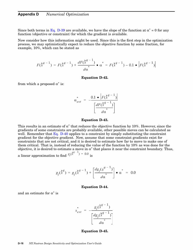
Appendix D Numerical Optimization
Since both terms in Eq. D-39 are available, we have the slope of the function at α* = 0 for anyfunction (objective or constraint) for which the gradient is available.
Now consider how this information might be used. Since this is the first step in the optimizationprocess, we may optimistically expect to reduce the objective function by some fraction, forexample, 10%, which can be stated as
Equation D-42.
from which a proposed α* is:
Equation D-43.
This results in an estimate of α* that reduces the objective function by 10%. However, since thegradients of some constraints are probably available, other possible moves can be calculated aswell. Remember that Eq. D-40 applies to a constraint by simply substituting the constraintgradient for the objective gradient. Now, assume that some constraint gradients exist forconstraints that are not critical, and it is desired to estimate how far to move to make one ofthem critical. That is, instead of reducing the value of the function by 10% as was done for theobjective, it is desired to estimate a move in α* that places it near the constraint boundary. Thus,
a linear approximation to find is
Equation D-44.
and an estimate for α* is
Equation D-45.
D-18 NX Nastran Design Sensitivity and Optimization User’s Guide

Numerical Optimization
Therefore, even at the beginning of the one-dimensional search, a considerable amount ofinformation is available to direct the process. Using the estimates for given by Eq. D-41 andEq. D-43 for each noncritical constraint, the smallest positive proposed is taken as the firstestimate of how far to move.
If constraints are currently violated, Eq. D-43 can still be used. Applying this approximation toall violated constraints, the largest proposed value of α* is selected as an estimate of how farto move to overcome all constraint violations. If the projected move to a constraint that is notcurrently active is smaller than this, then a move to that constraint is made as a first estimate,since we do not want to add new constraints to the set of violated constraints.
Using similar approximations, we can also estimate an upper bound on α* that forces all designvariables to their lower or upper bounds. This then provides a maximum allowable value for α*.
While this brief discussion is not detailed enough to cover all of the intricacies of estimatingthe first step in the one-dimensional search, it does provide a sense of the complexity of thedecision processes. AIso, it should be noted that on subsequent search directions, this processis modified to account for knowledge gained on previous iterations. For example, if an averageof 5% improvement is obtained on the last two one-dimensional searches, then another 5%improvement is attempted on this one.
The one-dimensional search process now proceeds to find the bounds on the α* that contain thesolution. Once the bounds on α* are known, the constrained minimum is found by interpolation.
Since has been defined as a direction of improving design, the search can be limited topositive values of α*.
D.4 Finding Bounds On α*At the beginning of this process, the values of the objective and constraints are known at α* =0 and α* = α1, where α1 is the initial estimate for α*. Following are three cases that must beconsidered when deciding if is the upper bound.
Case 1 - All constraints are initially satisfied (all gj(α* = 0) < CTMIN). In this case, the searchdirection is the one that reduces the objective. Therefore, if at α1, the objective is greater than atα0(α = 0), then α1 is an upper bound on α*. Also, since the initial constraints are all satisfied, ifany gj(α1) > CTMIN, then α1 is an upper bound, because the search has moved into the infeasibledesign space. If either the objective function has begun to increase or some constraint hasbecome violated, then α1 is chosen as the upper bound αu.
Case 2 - One or more constraints are violated (greater than CTMlN) at α* = 0, and the objectivefunction is increasing (dF(xq − 1)/dα* > 0). Here, a search direction has been chosen that shouldreduce the constraint violation. Thus, at α1, if the maximum constraint value is greater than themaximum constraint value at α* = 0, then α1 is the upper bound. This usually occurs when somenew constraint becomes violated at α1. If this happens, it is probably not possible to overcomethe constraint violations in this direction, but the maximum constraint violation may at least bereduced. Alternatively, a value of α1 might be found where all constraints are satisfied. If thishappens, a feasible design is found and so, again, α1 is an upper bound on α*. Here, there islittle concern that the objective function is increasing, since the first priority is to overcome theconstraint violations. If the constraint violations can be overcome, it is desirable to do so with aminimum increase in the objective function.
Case 3 - One or more constraints are violated (greater than CTMlN) at α* = 0, and the objectivefunction is decreasing (dF(xq − 1)/dα* > 0). This is the same as Case 2 except that the objectivefunction can be reduced. Therefore, everything is the same except that the search is notstopped if the constraint violation(s) are overcome. If a feasible design can be found that allows
NX Nastran Design Sensitivity and Optimization User’s Guide D-19

Appendix D Numerical Optimization
further reduction of the objective function, movement continues in this direction until somenew constraint becomes active or the objective begins to increase. The corresponding α* isthe upper bound αu.
During the process of finding the upper bound αu on α*, it may be required to move furtherthan the initial step α1. If α1 does not yield an upper bound, another step α2 = 2*α1 is takenand tried again. In practice, it may take many steps before a bound is found on the solution. Ifthis is the case, the best four solutions are retained and called αL, α1, α2, and αU. If more thanthree steps are required, the lower bound αL will not equal zero. Instead, a lower bound iscarried forward to retain the nearest four proposed values of α*. If fewer than four values areavailable (including α* = 0), then all are retained. For each retained value of α*, the value ofthe objective and all constraint functions are also retained. These are then used to interpolatefor an improved solution to the value of α*.
D.5 Interpolation for α*Once bounds on the solution to the one-dimensional search problem have been established, it isdesirable to refine the solution as much as possible. To achieve this, a polynomial interpolation ofthe objective and constraint functions is used. The basic tool used here is a simple polynomialcurve fit, which may be linear, quadratic, or cubic, depending on the amount of informationavailable. If more than four pieces of information are available, then higher order approximationscould be used. However, experience has shown that a cubic fit is adequate to approximate thefunctions without introducing too much numerical error.
Whether the objective function or a constraint is to be approximated, the basic approach is thesame. The process is demonstrated using a quadratic fit to three function values. The otherapproximations are similar and are explained in detail in Vanderplaats, “An Efficient FeasibleDirection Algorithm for Design Synthesis,”3.
A quadratic polynomial is defined as
Equation D-46.
where: a0, a1, a2 are constants, and ax is the variable.
In this case, x corresponds to the one-dimensional search parameter α*.
Next, assume that three values of F exist for three values of x, as listed in the table below:
x F0.5 –1.251.0 –3.002.0 –2.00
Substituting the values of F and x into Eq. D-44 results in three equations with three unknowns
Equation D-47.
D-20 NX Nastran Design Sensitivity and Optimization User’s Guide

Numerical Optimization
Equation D-48.
Equation D-49.
Solving for the values of a0, a1, and a2 results in
Equation D-50.
Substituting this into Eq. D-44 results in
Equation D-51.
Eq. D-49 can be used in different ways depending on whether the function F is the objective or aconstraint. First, assume that this is the objective function and we wish to find the value of xthat minimizes it. The function F has a minimum or maximum value when the derivative of Fwith respect to x is zero. Differentiating Eq. D-49 with respect to x yields:
Equation D-52.
Setting this to zero and solving for x gives a proposed solution x = 1.33. Substituting this intoEq. D-49 gives an estimated value of the function of F = 3.33. However, this is not sufficient toindicate that F is a minimum. The second derivative must also be considered, where
Equation D-53.
Since the result is positive, the proposed solution represents a minimum of F instead of amaximum.
Now, assume that the function to be approximated is a constraint. In this case, the value of xis sought that drives the function to zero (i.e., forces the design to a constraint boundary). Toachieve this, the value of x must be found that makes Eq. D-50 equal to zero. Setting Eq. D-49 tozero and solving for x yields
NX Nastran Design Sensitivity and Optimization User’s Guide D-21

Appendix D Numerical Optimization
Equation D-54.
For each of these values of x, the estimated value of F is zero. The question is: Which one shouldbe chosen? In this case, note that the initial value F(x = 0) is positive. Therefore,x = 0.2792 isa proposed lower bound on α*, since this overcomes the constraint violation (to a quadraticapproximation). Thus, this is a possible lower bound on α*, αL. However, more information isavailable. The value of the variable x = 2.3974 is the point at which the constraint again becomesviolated. Therefore, this value of x is a possible upper bound on α*, αU. This can be verified bycalculating the gradient of F at αL and αU to determine if it is negative at αL, (i.e., forcing gjto be more negative) and positive at αU (i.e., forcing gj to be violated). To verify this, simplysubstitute the values of x into Eq. D-50.
The optimization process leads to an estimate for α* for the minimum of the objective and thezero of one constraint. In this case, the constraint is initially violated so we have both a lowerand an upper bound on α*. However, we must also estimate values of α* for all constraints. Themaximum lower bound and the minimum upper bound define the range for the proposed solutionto the one-dimensional search. It may happen that the proposed upper bound is less than theproposed lower bound. If this happens, it usually means that for each proposed α* there are oneor more violated constraints. In this case, Eq. D-50 is used to minimize the maximum constraintviolation, and this decision overrides other conditions.
Let us assume that the polynomial approximation for the objective and all constraints is usedand concludes with a lower and upper bound on the constraint values so that the upper bound isgreater than the lower bound. (If no constraints are violated at α* = 0, this is the usual case.)Next a choice must be made as to which value of to select. If the search starts with violatedconstraints and the lower bound is less than the upper bound, either the lower bound is selected,or the value is chosen that minimizes the objective (assuming that it is between the lower andupper bounds). If no constraints are violated at α* = 0, the minimum proposed α* is selected fromthe α* that minimizes the objective and the α* that represents the upper bound.
As indicated by the difficulty in describing the one-dimensional search process, this is aparticularly complex part of the optimization process. The description given here is only a simpleoutline of the process. In practice, decisions must be made based on how many proposed valuesof α* are available using linear, quadratic and cubic curve fits to estimate the best value of themove parameter. Since it is impossible to predict all the possible combinations of the situationsthat may arise, this is necessarily a search process that is based more on experience than theory.The key is the need to consistently improve the design. If the absolute best solution does notappear during this one-dimensional search, further iterations provide other chances until theconvergence criteria are satisfied. This explains why more complex methods are not used (withtheir associated number of function evaluations and cost) during the one-dimensional search. Inthe optimization algorithm used in NX Nastran, the one-dimensional search process is somewhatmore sophisticated but basically follows the same process as outlined here.
At this point, the best search direction to improve the design has been determined and a searchconducted in that direction. The question now is: How can it be determined if the optimal designhas been achieved? The answer is based on the decisions that determine when to terminatethe optimization process.
D-22 NX Nastran Design Sensitivity and Optimization User’s Guide

Numerical Optimization
D.6 Convergence to the OptimumSince numerical optimization is an iterative process, one of the most critical and difficult tasks isdetermining when to stop. The optimization software uses several criteria to decide when to endthe iterative search process, and these are described here. It is important to remember that theprocess described in this section relates only to the solution of the approximate optimizationproblem. The number of cycles through the entire design process is controlled by other similarcriteria.
D.7 Maximum IterationsAs with any iterative process, a maximum iteration counter is included. The default for this is40 iterations (search directions). Usually, an optimum is found sooner than this; therefore, themaximum is mainly intended to avoid excessive computations.
D.8 No Feasible SolutionIf the initial design is infeasible (constraints are violated), the first priority is to overcome theseviolations and find a feasible solution. However, if there are conflicting constraints, a feasiblesolution may not exist. Therefore, if a feasible design is not achieved in 20 iterations, theoptimization process is terminated.
D.9 Point of Diminishing ReturnsProbably the most common situation is where the optimum is approached asymptotically.Therefore, while some progress is still being made, continued iterations are not justified. This isparticularly true in NX Nastran because this program is solving an approximate problem that isto be updated on the next design cycle. Here, two criteria are used. The first criteria requiresthat the relative change in the objective between iterations be less than a specified toleranceDELOBJ. Thus, the criteria is satisfied if:
Equation D-55.
The default value for DELOBJ is 0.001.
The second criteria is that the absolute change in the objective between the iterations is lessthan a specified tolerance DABOBJ. This criteria is satisfied if
Equation D-56.
The default value for DABOBJ is the maximum of and 1.0E-20.
NX Nastran Design Sensitivity and Optimization User’s Guide D-23

Appendix D Numerical Optimization
The reason for the two criteria is that if the objective function is large, the relative changebetween two successive iterations is an indication of convergence. However, if F(x) is a verysmall number, a relative change is not meaningful, and thus the absolute change controls theconvergence.
Often, no progress is made on one iteration, but significant progress is produced on the next.Therefore, one of these criteria is required to be satisfied on ITRMOP consecutive iterationswhere the default value of ITRMOP is 2. Recall that this default may be changed on theDOPTPRM Bulk Data entry.
D.10 Satisfaction of the Kuhn-Tucker ConditionsThe Kuhn-Tucker conditions necessary for optimality are stated in Eq. D-14 through Eq. D-17.In the uncommon case where there are no constraints, these conditions degenerate to thefamiliar case of the vanishing gradient of the objective. In practice, this is assumed to be true ifall components of the gradient are less than 0.001.
The usual optimization task in NX Nastran is that many constraints are imposed. In the processof finding a usable-feasible search direction, it is possible to detect if the Kuhn-Tucker conditionsare satisfied. If they are, the optimization process should be terminated. However, in practice,other considerations may affect the results. Remember that a constraint is defined as active if itis numerically greater than the parameter CT. The optimization starts with CT = 0.03. (Anyconstraint within three percent of being satisfied is called critical.) Since a constraint with thisvalue is considered in the Kuhn-Tucker calculations, these conditions may be satisfied even ifthe search is up to three percent away from the constraint boundary. Therefore, if CT is greaterthan CTMIN in magnitude, the CT value is reduced by some fraction (typically 50%) and anotherattempt can be made to find a usable-feasible direction. If CT is reduced in magnitude to avalue of –CTMIN, and can still satisfy the Kuhn-Tucker conditions, the optimization processis terminated.
D.11 Sequential Linear ProgrammingSequential Linear Programming (see 11) was briefly introduced in Section 1.3. This sectionpresents the method in greater detail.
The basic concept is actually quite simple. First, a Taylor Series approximation for the objectiveand constraint functions is created. This approximation is then used for optimization, instead ofthe original nonlinear functions. Now when the optimizer requires the values of the objectiveand constraint functions, these are very easily and inexpensively calculated from the linearapproximation. Also, since the approximate problem is linear, the gradients of the objective andconstraints are available directly from the Taylor Series expansion.
Traditionally, the SIMPLEX algorithm10 is used for solving the linear approximate problem.However, the optimizer in NX Nastran uses the Modified Method of Feasible Directions, since itsolves linear problems nicely and works well for the size of problems normally considered.
The general algorithm proceeds in the following steps:
1. For the current values of the design variables, sort the constraints and retain the mostcritical for use during this cycle. Typically, about 5 • NDV constraints are retained. The
10. Dantzig, G. B., Linear Programming and Extensions, Princeton University Press, Princeton, NJ, 1963.
D-24 NX Nastran Design Sensitivity and Optimization User’s Guide

Numerical Optimization
reason that all constraints are not retained is that there may be thousands, and most may befar from critical. Therefore, it would be wasted effort to calculate their gradients.
2. Create a first order Taylor Series expansion of the objective and retained constraints withrespect to the design variables.
3. Define move limits on the design variables. Typically, during one cycle, the design variableswill be allowed to change by 20-40%, but this is adjusted during later cycles.
4. Solve the linear approximate optimization problem.
5. Check for convergence. If satisfied, EXIT. Otherwise, repeat the process from step 1.
In step 1, Taylor Series expansions are created in the form:
Equation D-57.
Equation D-58.
Equation D-59.
and J is the set of retained constraints.
Note that everything in Eq. D-57 and Eq. D-58 is constant except the values of the design
variables, . Therefore, Eq. D-57 and Eq. D-58 can be rewritten as
Equation D-60.
Equation D-61.
Equation D-62.
NX Nastran Design Sensitivity and Optimization User’s Guide D-25

Appendix D Numerical Optimization
Equation D-63.
The following linear approximate optimization problem is now solved:
Equation D-64.
Equation D-65.
Equation D-66.
Equation D-67.
Equation D-68.
The multiplier D in Eq. D-67 and Eq. D-68 is initially set to RMVLMZ. Depending on theprogress of the optimization, this parameter will be sequentially reduced. Typically, the firstapproximate optimization produces a design that violates one or several constraints. However, asthe optimization proceeds, this constraint violation should be reduced. If it actually increases,then D is reduced, as well as the move limits on the design variables.
The convergence criteria for the SLP method are much the same as for the other methods, withthe addition that the process will not terminate if there are significant constraint violations. Inthis case, the process continues until the constraints are satisfied or the maximum number ofiterations is reached.
D-26 NX Nastran Design Sensitivity and Optimization User’s Guide

Numerical Optimization
D.12 Sequential Quadratic ProgrammingThis method is considered to be an excellent method by many theoreticians11 12.
The basic concept is very similar to Sequential Linear Programming. First the objectiveand constraint functions are approximated using Taylor Series Approximations. However, aquadratic, rather than a linear approximation of the objective function is used. Linearizedconstraints are used with this to create a direction finding problem of the form:
Equation D-69.
Equation D-70.
This sub-problem is solved using the Modified Method of Feasible Directions. The matrix B isa positive definite matrix that is initially the identity matrix. On subsequent iterations, B isupdated to approach the Hessian of the Lagrangian functions.
Now assume the approximate problem of minimizing Q subject to the linearized constraintshas been solved. At the optimum for this problem, the Lagrange multipliers λj j = 1, m can becalculated. With the Lagrange multipliers available, an approximate Lagrangian function can beconstructed and used to search in the direction defined by . The task is to find in order to:
Equation D-71.
where:
=
uj = |λj| j = 1, m first iteration
uj = j = 1, m subsequent iterations
and uj′ = uj from the previous iteration.
11. Powell, M. J. D., “Algorithms for Nonlinear Constraints that use Lagrangian Functions,” math. Prog., Vol. 14, No. 2, pp.224–248, 1978.,12. Vanderplaats, G. N. and Sugimoto, H., “Application of Variable Metric Methods to Structural Synthesis,” EngineeringComputations, Vol. 2, No. 2, June, 1985.
NX Nastran Design Sensitivity and Optimization User’s Guide D-27

Appendix D Numerical Optimization
During the one-dimensional search, approximations are made to the components of becausethis function has discontinuous derivatives at the constraint boundaries, but the componentsare smooth.
After the one-dimensional search is complete, the B matrix is updated using the BFGS formula;
Equation D-72.
where:
{p } =
{η} = θ{y} + (1 − θ)[B]{p}{y } = ∇x
q − ∇xq − 1
= if {p}T{y} ≥ 0,2{p}T[B]{p}
θ = if {p}T{y} < (0,2{p}T[B]{p})
Now [B*] replaces [B] and a new iteration is begun.
D.13 SummaryThe purpose of this Appendix has been to provide an overview of the computational detailsof the optimization process. The techniques used in the optimizer have been chosen becausethey are reasonably robust and because they allow for considerable flexibility in formulatingthe design problem.
From the variety of decisions that must be made during the optimization process it is clear thatanything the user can do to improve the numerical conditioning of the problem will have a stronginfluence on the efficiency and reliability of the result. It is hoped that some understanding ofthe actual optimization process will assist in this.
D-28 NX Nastran Design Sensitivity and Optimization User’s Guide