One Variable Calculus: Foundations and Applications One Variable Calculus: Foundations and...

One Variable Calculus: Foundations and Applications

Prof. Manuela Pedio

20550– Quantitative Methods for Finance

August 2018

About myself

2One Variable Calculus: Foundations and Applications

I graduated from Bocconi’s MSc in Finance in 2013 (yes, I remember what it is like to be in your shoes)

I have a four-year work experience in banking (as a derivatives sales analyst) before enrolling in a Ph.D.

I cooperate closely with prof. Guidolin (you will meet him in the next few days) so that we will see each other again during the year … (I am also his assistant in his role as MSc Director)

If you want to contact me look at my Bocconi’s page to find out office hours and my email:

http://didattica.unibocconi.it/docenti/cv.php?rif=196456

Objectives of the Course


The objective of this (prep)-course is to review a number of fundamental concepts from calculus and optimization with a selection of applications to economics and finance

In my part, I listed three books in the syllabus, the first two of them are substitutes:

Mathematics for Economists by Blume and Simon (BS) (classical book to teach mathematics for economists)

Fundamental Methods of Mathematical Economics by Chiang (C) (similar to Blume and Simon)

But dozens of other textbooks that you may have already used in your previous studies may do the job

Advanced Modelling in Finance Using Excel and VBA by Jackson and Staunton (JS) (highly enjoyable book about financial modelling in Excel)

Outline of the Course


Lectures 1 and 2 (3 hours, in class):

Linear and non-linear functions on ℝ

Limits, continuity, differentiability, rules to compute derivatives, approximation with differentials

Logarithmic and exponential functions

Introduction to integration

Lecture 3 (1.5 hours, in the lab):

Review of matrix algebra with applications in Excel

Lectures 4 and 5 (3 hours, 1.5 of which in the lab):

Introduction to optimization: functions of one variable

Generalization: functions of several variables

Use of Excel Solver for constrained optimization

Warm up: a bit of definitions (1/2)


FUNCTIONS ON ℝ: A function of a real variable x with domain D is a rule that assigns a unique real number to each number x in D

We typically use letters like f or g to denote such a rule

For the time being, we will consider f: ℝ → �, with � ⊂ ℝ, that is, functions from ℝ to ℝ

Usually, y = f(x) denotes the value that the function f assigns to the real number x belonging to its domain, or, in other words, the “value of f at x”

As an example, f(x) = x+1 is a function that assigns to each x of the domain, a number that is one unit larger; for instance, f(2) = 3 is the value of this function at 2

Ran

ge

Domain

Warm up: a bit of definitions (2/2)


The domain is the set of numbers x at which f(x) is defined

Typically, when the domain is not specified, we assume that it includes all the real numbers for which the function takes meaningful values

For instance, for the function � � =�

��the domain will be

−∞ ,−3 ∪ −3,∞ , that is, -3 is excluded from the domain

The range (or co-domain) of a function is instead the set of the values assumed by the function

As an example, the domain of f: � � = � is equal to the entire ℝ but the range is equal to ℝ�

Warm up: composition of functions


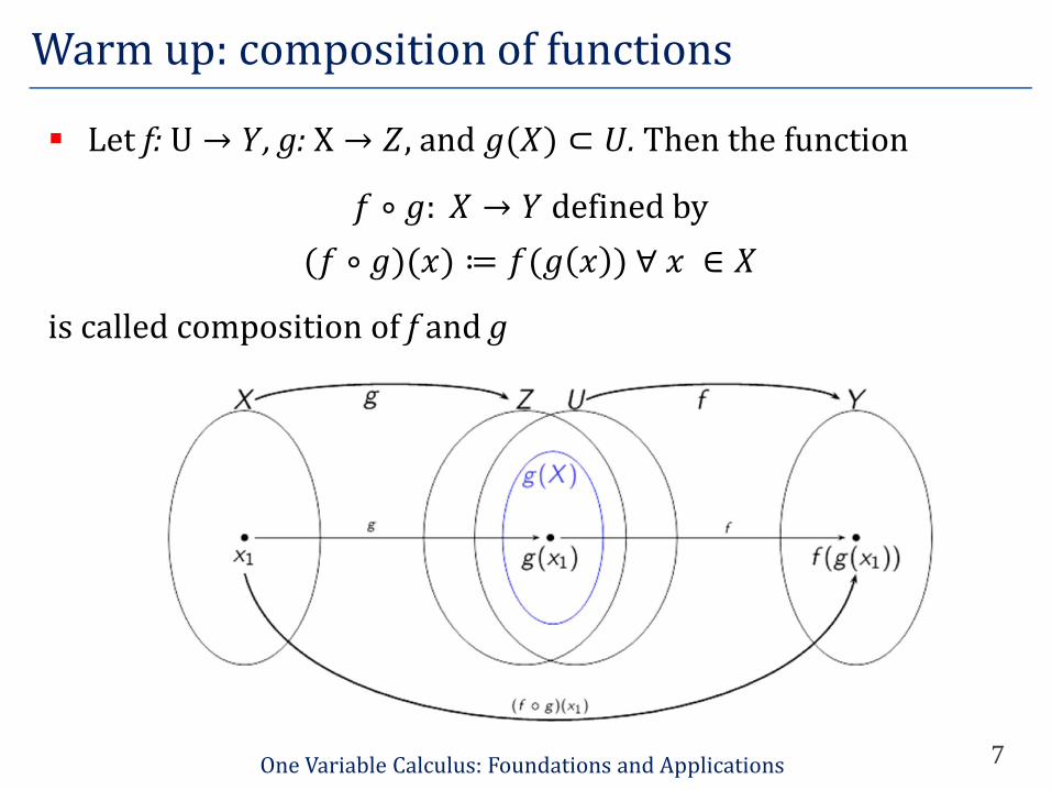
Let f: U → �, g: X → �,and �(�)⊂ � . Then the function

� ∘�: � → � defined by

(� ∘�)(�)≔ �(� � ) ∀ � ∈ �

is called composition of f and g

Figure 1

Basic geometric properties of a function (1/2)


The basic geometric properties of a function are whether it is increasing or decreasing and the location of its local and global minima and maxima (if any)

A function f is increasing if �� > �� implies �(��)> �(��)while a function f is decreasing if �� > �� implies �(��)<�(��)

The function depicted in Figure 1 is decreasing over ℝ� and increasing over ℝ�

The point where the function turns from decreasing to increasing is a (global) minimum for this function,in this case zero

Figure 2

Basic geometric properties of a function (2/2)


The function depicted in Figure 2 is increasing over ℝ� and decreasing over ℝ�

The point where the function turns from decreasing to increasing, is a (global) maximum for this function, here zero

If a function f changes from decreasing to increasing at ��, the point (��,�( ��)) is a local minimum of the function f; if �(�)≥ �(��)for all x then the point is a global minimum

If a function f changes from increasing to decreasing at ��, the point (��,�( ��)) is a local maximum of the function f; if �(�)≤ �(��)for all x then the point is a global maximum

We will come back to these notions when we speak of optimization

Different functions


The simplest functions are the monomials, those functions whichcan be written as � � = �� for some number a (coefficient)and some positive integer k, where k is said to be the degree ofthe monomial

For instance � � = 6�� is a monomial of the second order

A polynomial is a function formed by adding up differentmonomials; the degree of the polynomial is highest degree of anymonomial that appears in the function

For instance � � = 6��+2x is a polynomial of the third order

Rational functions are ratios of polynomials, e.g., � � =��+��

Non algebraic functions: exponential functions (where x appearsat the exponent), trigonometric functions, logarithmic functions,etc. (I will focus on exponential and logarithmic functions later on)

Examples of popular functions (1/2)


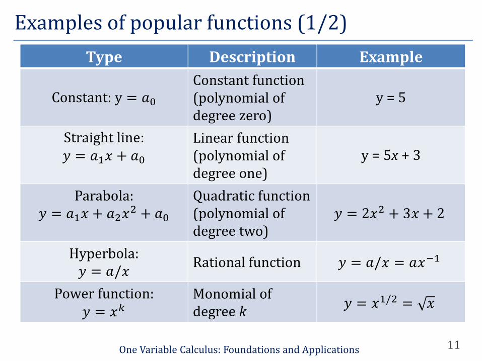
Type Description Example

Constant: y = ��

Constant function (polynomial of degree zero)

y = 5

Straight line: � = �� + ��

Linear function (polynomial of degree one)

y = 5x + 3

Parabola:� = �� + ��

� + ��

Quadratic function (polynomial of degree two)

� = 2�� + 3� + 2

Hyperbola:� = �/�

Rational function � = �/� = ��

Power function:� = ��

Monomial of degree k

� = ��/� = �

Examples of popular functions (2/2)


Power

Limits: a short detour (1/4)


To get a first intuition of the concepts of limit consider that afunction f is defined for all x near a but not necessarily at � = �

We say that the function f(x) has the number A as its limit as xtends to a if f(x) tends to A when x tends to a

We write

It is possible that the value of f(x) does not tend to any fixednumber as x tends to a; then we say that f(x) does not have a limitas x tends to a

lim�→�

� � = �



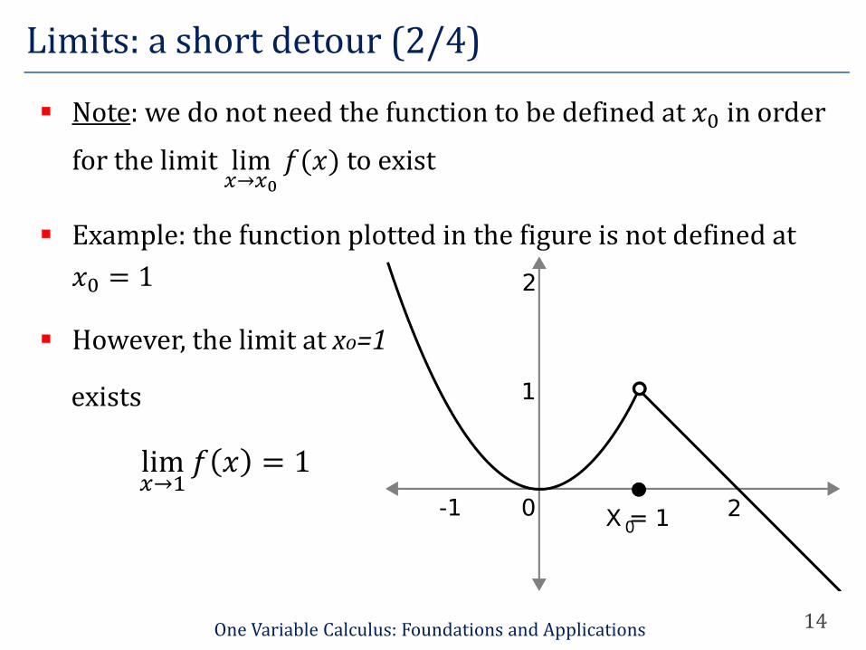
Note: we do not need the function to be defined at �� in order

for the limit lim�→��

�(�)to exist

Example: the function plotted in the figure is not defined at

�� = 1

However, the limit at xo=1

exists

lim�→�

� � = 1



Exercise: compute

lim�→��

�� + 5�



lim�→��

�� + 5�

x 1.800- 1.900- 1.990- 2.000- 2.001- 2.010- 2.100- 2.200-

f(x) -5.76 -5.89 -5.99 -6.001 -6.01 -6.09 -6.16

Numerical solution (with excel)

Using the rules

The slope of functions (1/4)


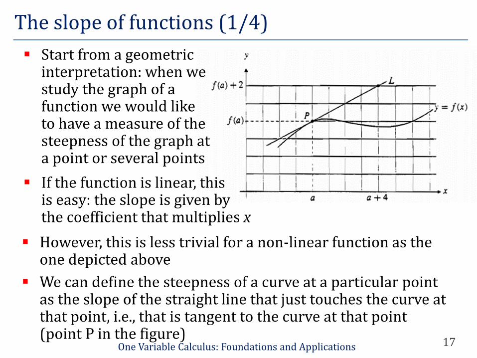
Start from a geometric interpretation: when we study the graph of a function we would like to have a measure of the steepness of the graph at a point or several points

If the function is linear, this is easy: the slope is given by the coefficient that multiplies x

However, this is less trivial for a non-linear function as the one depicted above

We can define the steepness of a curve at a particular point as the slope of the straight line that just touches the curve at that point, i.e., that is tangent to the curve at that point (point P in the figure)

The slope of curves (2/4)


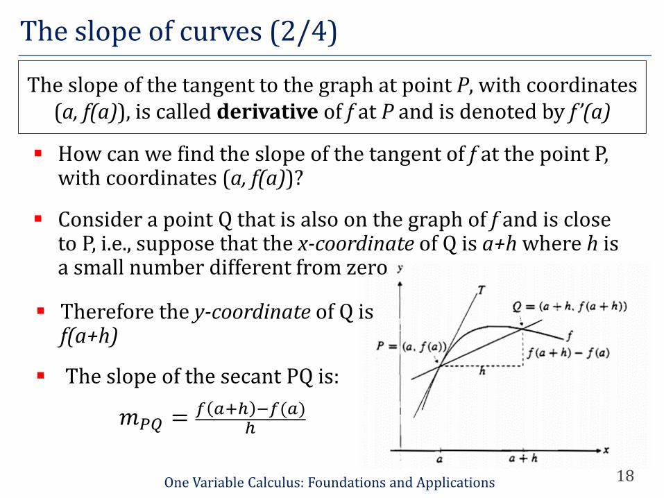
How can we find the slope of the tangent of f at the point P,with coordinates (a, f(a))?

Consider a point Q that is also on the graph of f and is close to P, i.e., suppose that the x-coordinate of Q is a+h where h is a small number different from zero

The slope of the tangent to the graph at point P, with coordinates (a, f(a)), is called derivative of f at P and is denoted by f ’(a)

Therefore the y-coordinate of Q is f(a+h)

The slope of the secant PQ is:

�� = � �� (�)�



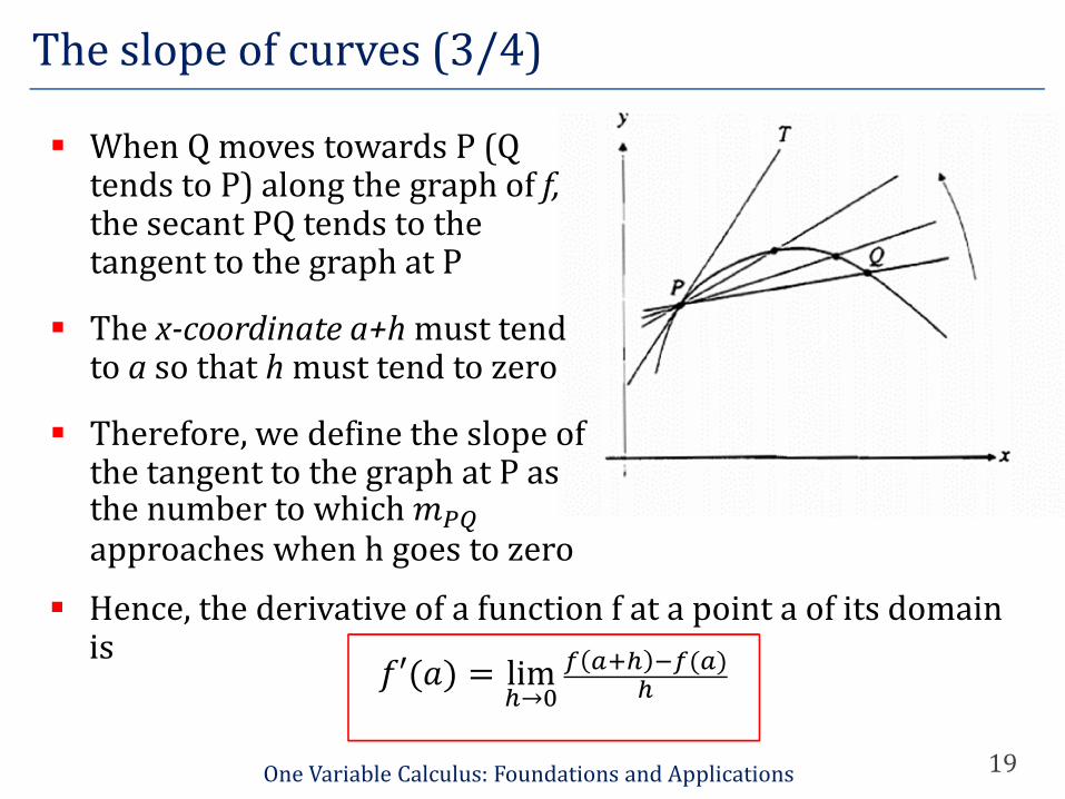
When Q moves towards P (Q tends to P) along the graph of f, the secant PQ tends to the tangent to the graph at P

The x-coordinate a+h must tend to a so that h must tend to zero

Therefore, we define the slope of the tangent to the graph at P as the number to which ��

approaches when h goes to zero

�′(�)= lim�→�

� �� (�)�

Hence, the derivative of a function f at a point a of its domain is



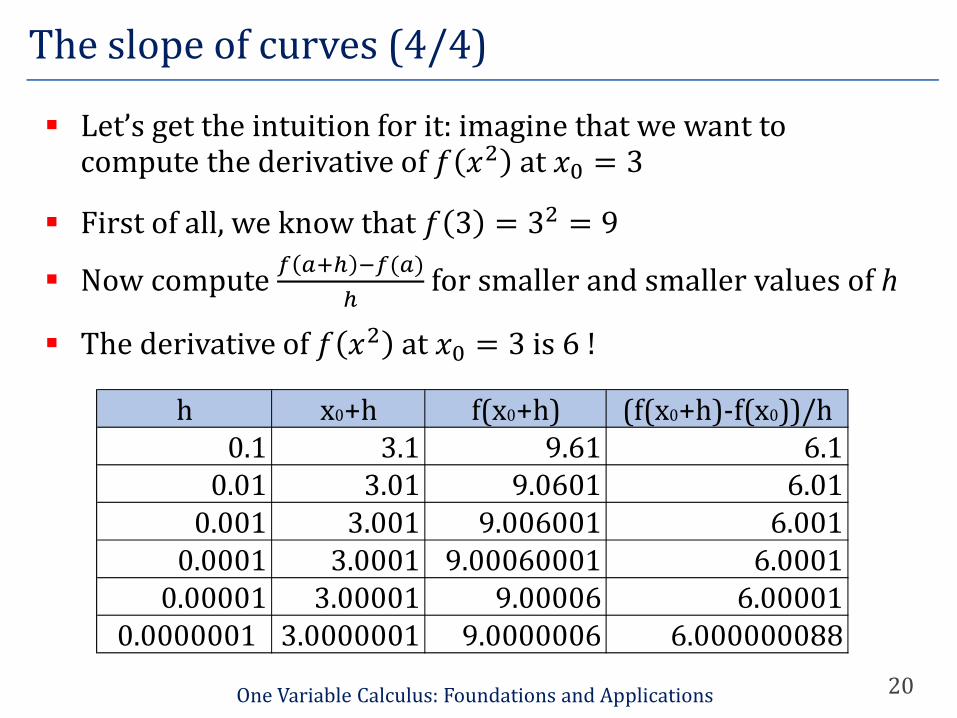
Let’s get the intuition for it: imagine that we want to compute the derivative of � �� at �� = 3

First of all, we know that � 3 = 3� = 9

Now compute � �� (�)

�for smaller and smaller values of h

The derivative of � �� at �� = 3 is 6 !

h x0+h f(x0+h) (f(x0+h)-f(x0))/h0.1 3.1 9.61 6.1

0.01 3.01 9.0601 6.010.001 3.001 9.006001 6.001

0.0001 3.0001 9.00060001 6.00010.00001 3.00001 9.00006 6.00001

0.0000001 3.0000001 9.0000006 6.000000088

Interpretation of derivatives


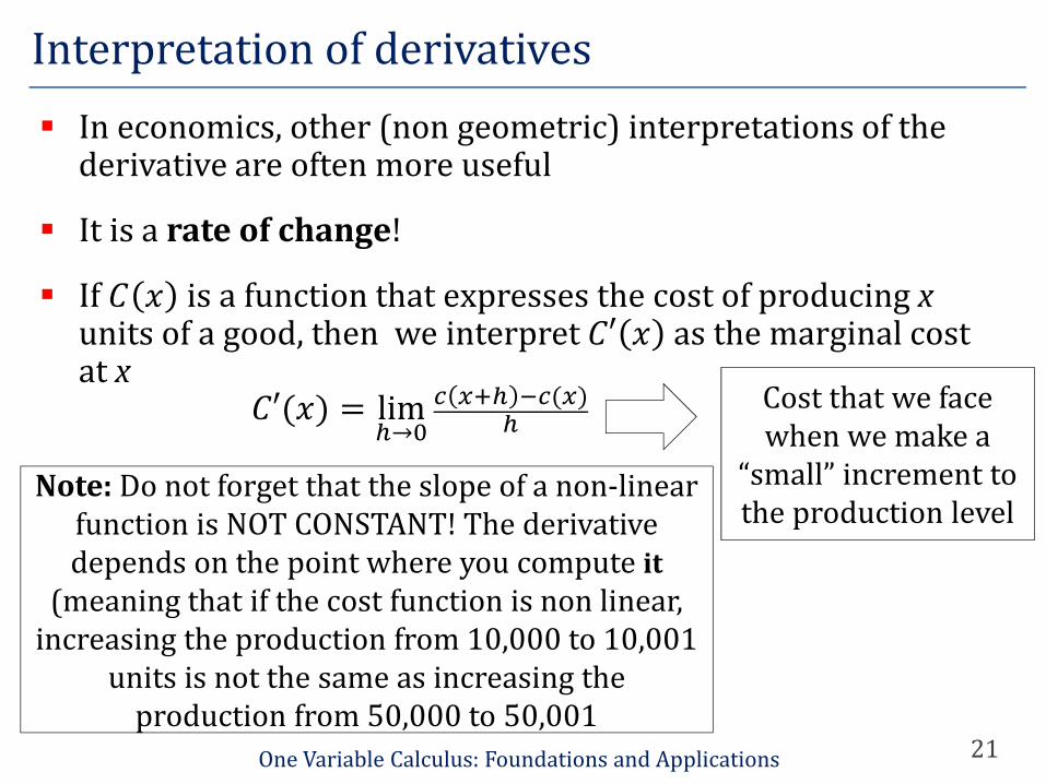
In economics, other (non geometric) interpretations of the derivative are often more useful

It is a rate of change!

If � � is a function that expresses the cost of producing x units of a good, then we interpret �′ � as the marginal cost at x

�′(�)= lim�→�

� �� (�)�

Cost that we face when we make a

“small” increment to the production level

Note: Do not forget that the slope of a non-linear function is NOT CONSTANT! The derivative depends on the point where you compute it

(meaning that if the cost function is non linear, increasing the production from 10,000 to 10,001

units is not the same as increasing the production from 50,000 to 50,001

Rules for computing derivatives (1/2)


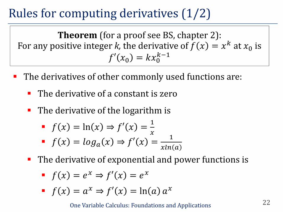
Theorem (for a proof see BS, chapter 2): For any positive integer k, the derivative of � � = �� at �� is

�′ �� = ��

The derivatives of other commonly used functions are:

The derivative of a constant is zero

The derivative of the logarithm is

� � = ln � ⇒ �′ � =�

�

� � = �� ⇒ �′ � =�

��

The derivative of exponential and power functions is

� � = �� ⇒ �′ � = ��

� � = �� ⇒ �′ � = ln � ��

Rules for computing derivatives (2/2)


CHAIN RULE: � � � = �� ′(�)

Exercises


Take the derivatives of the following functions:

−7�� + 2� + 1 ⇒ −28�� +�

�

��

��⇒

��

(��)�

ln 3� + 2 ⇒�

��3

ln � 5� ⇒�

�5� + ln � 5

��

��⇒

��(��)� ��

(��)�

��

��⇒

�� (��)

(��)�

ln �� =�

�3

Exercise (Solutions)


Take the derivatives of the following functions:

−7�� + 2� + 1 ⇒ −28�� +�

�

��

��⇒

��

(��)�

ln 3� + 2 ⇒�

��

ln � 5� ⇒�

�5� + ln � 5

��

��⇒

��(��)� ��

(��)�

��

��⇒

�� (��)

(��)�

ln �� =�

�

One Variable Calculus: Foundations and Applications One Variable Calculus: Foundations and...

Documents

Transcript of One Variable Calculus: Foundations and Applications One Variable Calculus: Foundations and...