One-particle and few-particle billiards - University of Oxford · One-particle and few-particle...

CHAOS 16, 013129 �2006�

Dow

One-particle and few-particle billiardsSteven LanselSchool of Electrical and Computer Engineering and School of Mathematics,Georgia Institute of Technology, Atlanta, Georgia 30332-0160

Mason A. PorterDepartment of Physics and Center for the Physics of Information, California Institute of Technology,Pasadena, California 91125-3600

Leonid A. BunimovichSchool of Mathematics and Center for Nonlinear Science, Georgia Institute of Technology,Atlanta, Georgia 30332-0160

�Received 29 August 2005; accepted 3 November 2005; published online 30 March 2006�

We study the dynamics of one-particle and few-particle billiard systems in containers of variousshapes. In few-particle systems, the particles collide elastically both against the boundary andagainst each other. In the one-particle case, we investigate the formation and destruction of reso-nance islands in �generalized� mushroom billiards, which are a recently discovered class of Hamil-tonian systems with mixed regular-chaotic dynamics. In the few-particle case, we compare thedynamics in container geometries whose counterpart one-particle billiards are integrable, chaotic,and mixed. One of our findings is that two-, three-, and four-particle billiards confined to containerswith integrable one-particle counterparts inherit some integrals of motion and exhibit a regularpartition of phase space into ergodic components of positive measure. Therefore, the shape of acontainer matters not only for noninteracting particles but also for interacting particles. © 2006American Institute of Physics. �DOI: 10.1063/1.2147740�

In this paper, we conduct a numerical investigation ofone-particle systems (billiards) with regular, chaotic, andmixed (regular-chaotic) dynamics and of small numbers(two, three, and four) of elastically colliding particles(balls) confined to the same billiard tables. Thus, this re-port differs essentially from traditional numerical studiesof systems of interacting particles, which deal with manyparticles confined to containers of the simplest shapes[usually boxes, or boxes with periodic boundary condi-tions (i.e., tori)]. Using the simple example of hard ballsin a circle, we demonstrate that systems of interactingparticles need not be ergodic. Therefore, the recently dis-covered typical inhomogeneity of stationary distributionsof noninteracting particles in containers may well be ineffect for interacting particles as well. We also comparethe dynamics of few-particle systems with their one-particle counterparts when the dynamics of the latter isregular, chaotic, and mixed.

INTRODUCTION

Two major 20th century discoveries completely trans-formed scientists’ understanding of nonlinear phenomena.One was Kolmogorov-Arnold-Moser �KAM� theory, whichdemonstrated the stability of regular dynamics for small per-turbations of Hamiltonian systems.1–4 The other was thetheory of stochasticity of dynamical systems �loosely called“chaos theory”� which demonstrated the stability of stronglyirregular dynamics under small perturbations.5–7

Typical Hamiltonian systems have mixed dynamics, with
islands of stability �“KAM islands”� situated in a chaotic sea.
1054-1500/2006/16�1�/013129/12/$23.00 16, 01312

nloaded 31 Mar 2006 to 131.215.106.179. Redistribution subject to A

However, rigorous mathematical investigations of such sys-tems are notoriously difficult because different analyticalmethods have been developed for systems with fully regularor fully chaotic dynamics. Both approaches fail at the bound-aries between chaotic and regular regions. Numerical inves-tigations of systems with mixed dynamics are also difficultfor the same reason �small islands are not easy to find/observe numerically�.

There have been numerous attempts to find Hamiltoniansystems with mixed dynamics �divided phase space� that al-low an exact, rigorous analysis.8–10 Recently, unexpectedlysimple and visual examples of such systems were found inthe form of mushroom billiards, whose geometry generalizesthe long-studied stadium billiard.11,12 From a mathematicalperspective, the discovery of mushroom billiards has nowmade it possible to address some delicate questions about thedynamics of systems with coexisting KAM islands and cha-otic regions.11–13 Such theoretical studies can be readilytested experimentally in many physical situations. For ex-ample, two-dimensional billiards in essentially arbitrary ge-ometries corresponding to systems with integrable, chaotic,and mixed dynamics can be constructed using microwavecavities,14–16 quantum dots,17 and atom optics.18–20 The prob-lems that can be studied by experimentalists using billiardsystems are both fundamental and diverse, ranging from thedecay of quantum correlations18 to investigations of the dy-namics of Bogoliubov waves for Bose-Einstein condensatesconfined in various billiard geometries.20

In this work, we investigate chaos-chaos transitions in
classical billiard systems. To do this for a given billiard, we
© 2006 American Institute of Physics9-1

IP license or copyright, see http://chaos.aip.org/chaos/copyright.jsp

http://dx.doi.org/10.1063/1.2147740

http://dx.doi.org/10.1063/1.2147740

013129-2 Lansel, Porter, and Bunimovich Chaos 16, 013129 �2006�

Dow

gradually perturb its geometry, just as one would for theorder-chaos transitions that have long been studied in Hamil-tonian systems. In this case, however, the billiard’s phasespace has chaotic regions both before and after the perturba-tion rather than just after it. We examine the proliferation anddestruction of KAM islands that result from these perturba-tions and consider the concomitant disappearance and ap-pearance of chaotic regions in phase space. In particular, weinvestigate the example of one-particle generalized mush-room billiards. We also study few-particle billiards, in whichthe confined particles collide elastically not only against theboundary but also against each other. Towards this end, westudy them in geometries whose associated one-particle bil-liard dynamics are integrable, chaotic, and mixed. We con-sider particles of different sizes to examine the limit in whichthe particles become smaller and the few-particle system be-comes more like the associated one-particle billiard.

Traditional mathematical studies of systems of particlesdeal either with just one particle �billiards and perturbations/modifications thereof� or with an infinite number of particles.Numerical studies have been concerned with hundreds orthousands �or more� interacting particles.21–23 Another tradi-tion for studies of systems of interacting particles is to focuson the potential governing interactions between particlesrather than on the shape of the containers in which the par-ticles are confined; systems of interacting particles have tra-ditionally been considered in a box or a torus.

However, from both the theoretical and practical stand-points, systems of just a few particles are getting increasingattention, in large part because of nanoscience and possibleapplications in nanotechnology. From an experimental per-spective, collisions between particles can be studied usingthe framework of cold atoms.19,24 On the theoretical side, itwas recently demonstrated that stationary distributions ofsystems of noninteracting particles in containers with non-trivial shapes are typically very inhomogeneous.12 A naturalquestion that consequently arises is whether such phenomenamay occur in systems of interacting particles. In this paper,we give a positive answer to this question by demonstratingthat the same effect is present in systems of two, three, andfour hard balls in a circle.

The structure of this paper is as follows. First, we exam-ine the dynamics of one-particle billiards. We give somebackground information on integrable and chaotic billiardsbefore turning our attention to billiard systems with mixedregular-chaotic dynamics. We consider, in particular, billiardgeometries shaped like mushrooms and generalized mush-rooms. We then study the dynamics of two-particle billiardsin containers whose corresponding one-particle billiard dy-namics are integrable, chaotic, and mixed. We subsequentlyexamine three-particle and four-particle billiards.

ONE-PARTICLE BILLIARDS

Classical �one-particle� billiard systems are among thebest-studied Hamiltonian dynamical systems.25,26 The dy-namics of a billiard is generated by the free motion of aparticle �usually taken to be a point� inside a closed domainQ with piecewise smooth boundary �Q in Euclidean space

d
R . �Most studies concentrate on the case d=2.� The con-

fined particle collides elastically against the boundary, so theangle of incidence equals the angle of reflection.

The billiard flow St has phase space M= ��q ,v� :q�Q , �v�=1�. The unit normal vector �pointing towards theinterior of the billiard� to �Q at the regular point q��Q isdenoted n�q�. Also, let zª�q ,v� denote a point in phasespace.

A natural projection of M into its boundary is M= ��q ,v� :q��Q , �v�=1, �v ,n�q��0�, where �·,· denotesthe standard inner product. Define the billiard map T byT�q ,v�= �q1 ,v1�, where q1 is the point of �Q at which theoriented line through �q ,v� first hits �Q and v1=v−2�n�q1� ,vn�q1� is the velocity vector after the reflectionagainst the boundary at the point q1. �The billiard map is notdefined if q1 is at a singular point of �Q.� When d=2, thismap is parametrized according to the arc length s along �Q�measured from an arbitrary point on �Q� and the angle �between v and n�q�. Hence, �� −� /2 ,� /2� and �n�q� ,v=cos �. The billiard flow conserves the volume measure d�in M. The corresponding invariant measure for T is d�=A cos �dsd�, where A=1/ �2 length��Q�� is a normaliza-tion constant.

Billiards with fully integrable or chaotic dynamics

A curve ��Q is called a caustic of the billiard if when-ever any link of some trajectory is tangent to �, then all otherlinks of the same trajectory are also tangent to �. It is well-known that the configuration space of a billiard in a circle iscontinuously foliated by circles concentric to �Q. A circularbilliard is thus completely integrable. Elliptical billiards aresimilarly integrable, although they have two continuousfamilies of caustics instead of just one. One family is formedby trajectories tangent to confocal ellipses, and the other isformed by trajectories tangent to confocal hyperbolae. In thelimit of zero eccentricity, the hyperbolic caustics disappearand the elliptical caustics become concentric circular caus-tics. Semicircles and semiellipses are likewise integrable.27

Examples of chaotic billiards include dispersing billiardssuch as the Sinai and diamond containers28 and billiards withfocusing boundaries such as stadia. Neighboring parallel or-bits diverge when they collide with dispersing components ofa billiard’s boundary. In chaotic focusing billiards, on theother hand, neighboring parallel orbits converge at first, butdivergence prevails over convergence on average. �Hence,chaotic billiards with focusing boundaries may be viewed asoccupying an intermediate position between dispersing andintegrable billiards.� Divergence and convergence are bal-anced in integrable billiards.

The investigation of chaotic billiards has a long history.The flow in classical chaotic billiards is hyperbolic, ergodic,mixing, and Bernoulli.26,28 Autocorrelation functions ofquantities such as particle position and velocity of confinedparticles decay exponentially.23,29 Additionally, the quantiza-tions of classically chaotic billiards bear the signatures ofclassical chaos in, for example, the distributions of their en-ergy levels, the “scarring”/“antiscarring” �increased/

2
decreased wave function density � � that corresponds to

013129-3 One-particle and few-particle billiards Chaos 16, 013129 �2006�

Dow

classical unstable/stable periodic orbits, and the structure ofnodal curves �at which the density vanishes�.30–32

Billiards with mixed dynamics

Typical Hamiltonian systems exhibit mixed regular-chaotic dynamics �divided phase space�. Examples of billiardgeometries that yield such dynamics include nonconcentricannuli �with circular boundaries�10 and ovals.8 For systemswith mixed dynamics, however, it is generally difficult toexactly determine and describe the structure of the bound-aries of stability islands. A container shaped like a mushroomprovides an example of a billiard with divided phase spacefor which such precise mathematical analysis is feasible.11–13

One reason it is natural to investigate mushroom billiardsand their generalizations is that they can be designed in a

FIG. 1. �Color online� Configuration space �a� �in continuous time� andphase space �b� �in discrete time� plots for an elliptical mushroom billiardwith a rectangular stem. The semimajor and semiminor axes of the mush-room’s elliptical cap have respective lengths of 2 and 1. The stem has height3 and width 1. In panel �b�, the horizontal axis indicates the location of aboundary collision, as measured by the arc length �with an extra scalingalong the elliptical portion of the mushroom’s cap� in the clockwise direc-tion from the right-most point of the table. The vertical axis indicates theincident angle of the particle’s collisions with the boundary. To illustratehow to read subsequent figures in this paper, we have plotted a trajectory �inred/gray� that enters the mushroom’s stem and another one �in black� thatdoes not. We label the regions in �b� to help identify their correspondingboundary arcs in �a�. �Regions matched to different arcs are separated in �b�by vertical lines, which correspond to singular points of the billiard bound-ary.� For example, collisions against the elliptical arc of the mushroom’s capoccur in region 6 �the right-most region� of phase space.

precise manner so that they have an arbitrary number of in-


tegrable and chaotic components, each of which occupies thedesired fraction of the phase space volume. Their study maythus lead to a better understanding of Hamiltonian systemswith divided phase space.

A circular mushroom billiard consists of a semicircularcap with a stem of some shape attached to the cap’s base.Circular mushroom billiards provide a continuous transitionbetween integrable �semi�circular billiards and chaotic�semi�stadium billiards. In circular mushrooms, trajectoriesthat remain in the cap are integrable, whereas those that enterthe stem are chaotic �except for a set of measure zero�. Theprecise characterization of all such trajectories is completelyunderstood, and one can change the dimensions of the mush-room to controllably alter the relative volume fractions inphase space of initial conditions containing integrable andchaotic trajectories. Another interesting property of circularmushroom billiards, which was demonstrated recently, is thatthey exhibit “stickiness” in their chaotic trajectories �charac-terized by long tails in recurrence-time statistics� even

13

FIG. 2. �Color online� Periodic orbits of the elliptical mushroom from Fig.1. �a� Trajectory near a stable, symmetric periodic orbit of period 34 �me-dium gray�. �b� Trajectory near a stable, asymmetric periodic orbit �lightgray�.

though they do not possess hierarchies of KAM islands.


eriod


Dow

In this section, we investigate �axially symmetric� ellip-tical mushroom billiards, which generalize the elliptical sta-dium billiard33,34 and consist of a semiellipse with a stemextending from the center of its major �horizontal� axis. First,we show with an example plot �Fig. 1� how to visualize thedynamics in both configuration space and phase space. Uti-lizing mushrooms with several stem geometries �rectangular,triangular, and trapezoidal�, we subsequently examine sym-metric and asymmetric periodic orbits and illustrate the birthand death of KAM islands that occur as the stem height isincreased. As an example, we derive analytically the stemheight at which the period-2 orbit along the mushroom’s axisof symmetry becomes unstable.

To study the dynamics of elliptical mushroom billiards,we conducted extensive numerical experiments using soft-ware that we wrote and have made publicly available.35 Toillustrate subsequent plots, we depict in Fig. 1 the billiardsystem in configuration and phase space for the case of arectangular stem. We then show the dynamics of two of this

FIG. 3. �Color� Divided phase space and periodic orbits of an elliptical mussemiminor axes have lengths 2 and 1, respectively. The triangular stem hasdepicts 13 initial conditions. �b� Trajectory near a stable, symmetric periodperiodic orbit of period 10 �shown in gray�. �d� Phase space depicting the p

billiard’s trajectories in Fig. 2. The phase space of this bil-


liard is divided, as it has both regular and chaotic regions. Inmushroom billiards with rectangular stems, we observestable periodic orbits of arbitrary length.

We also study elliptical mushrooms with triangular �seeFig. 3� and trapezoidal stems �no figures shown�. When out-side the “extended stem” of the mushroom, trajectories be-have in the same manner regardless of the shape of the stem.�The extended stem of a mushroom billiard consists of thestem itself plus the portion of the hat inside the largest geo-metrically similar semiellipse concentric to the hat thattouches an upper corner of the stem.� Differences in dynam-ics for mushrooms with different stems manifest only fortrajectories that enter the extended stem �and hence the stemper se�. For example, mushroom billiards with trapezoidalstems possess nontrivial periodic orbits that never leave thestem. In contrast, there are no such periodic orbits for mush-room billiards with triangular stems and only trivial orbits ofthis kind for mushrooms with rectangular stems.

Symmetric mushroom billiards with rectangular, triangu-

billiard with a stem shaped like an isosceles triangle. The semimajor andight and width of 1. �a� Phase space showing multiple islands. The figureit of period 14 �shown in black�. �c� Trajectory near a stable, asymmetricic orbits from �b� and �c�.

hrooma he

ic orb

lar, and trapezoidal stems all have stable symmetric and



Dow

asymmetric periodic orbits that traverse both the hat and thestem. For triangular and trapezoidal stems, asymmetric peri-odic orbits that enter the stem are one of two types: �1� thetrajectory collides against the stem near one of its bottomcorners; or �2� the trajectory collides against a line segmentthat is perpendicular to the current link of the trajectory. �Inthe latter case, the particle then turns around and begins totrace its path backwards.� Rectangular stems, however, onlyhave orbits of type 1. These orbits return to the cap from thestem at the same angle at which they left, with resultingboundary collisions in the cap as if the trajectory hadbounced once off a linear segment perpendicular to the tra-jectory rather than bouncing several times in the stem �see,for example, Fig. 2�b��. Such trajectories enter the stem,bounce around against the stem’s boundary, and then emergefrom it in the same fashion that they entered. By contrast,

FIG. 4. �Color� Magnifications of phase space showing the disappearance ofthe central KAM island—which corresponds to the vertical period-2 trajec-tory passing through the axis of symmetry of the elliptical mushroom—as aresult of varying the stem height. The example depicted has a semimajoraxis of length 2, a semiminor axis of length 1, and a rectangular stem ofwidth 1. The central island disappears at stem height 3 �when the trajectorybecomes unstable�. The figure panels show an enlargement of the portion ofphase space corresponding to collisions with the elliptical arc. �a� Stem
height 2.5. �b� Stem height 3.

FIG. 5. �Color online� Distribution of incident angle for collisions betweenparticles and boundary for two identical particles of varying radius confinedin a circle of radius 1. The initial conditions for the three plots are shown inthe last row of Table I and discussed in the text. We simulate this systemthrough 200 000 total collisions of either particle with the boundary. �Thesedistributions count multiplicities for consecutive particle-boundary colli-sions, the incident angles of which are the same because there are no inter-vening particle-particle collisions.� �a� Particle radius 1/4. �b� Particle radius
1/10. �c� Particle radius 1/20.


Dow

type 1 asymmetric periodic orbits in triangular stems do nothave this property �see, for example, Fig. 3�c��. This differ-ence in dynamics reveals the presence of periodic orbits inmushroom billiards with rectangular stems that are notpresent in ones with triangular stems. For symmetric periodicorbits, we observe a similar reflection property for all threetypes of stems, except that there is an additional horizontalreflection in the trajectory’s return from the stem to the cap.Such trajectories �see Figs. 2�a� and 3�b�� result in periodicorbits that are present in all three families of mushroom bil-liards. No matter what they do inside the stem, such orbitsleave the stem with the same angle �ignoring sign� with re-spect to the mushroom’s axis of symmetry that they hadwhen they entered.

Numerous bifurcations occur with changes in stemheight, as KAM islands rapidly proliferate and change con-figurations. For instance, using triangular stems of width 1and heights ranging from 0.1 to 2.0 in increments of 0.1, weobserved a large variation in the number of central islandsappearing vertically down the left side of phase space �cor-responding to collisions against the billiard stem�. For ex-ample, there are six such islands in Fig. 3�a�. In some con-figurations, the islands correspond to two differenttrajectories: an asymmetric trajectory and its horizontal re-flection. In other configurations, one symmetric trajectoryhits all the islands. We observed similar phenomena for trap-ezoidal stems with lower width 1.5, upper width 0.5, andheights ranging from 0.1 to 2.0 �in increments of 0.1�.

The bifurcation from stability to instability for the peri-odic vertical trajectory in symmetric elliptical mushrooms�for stems with a neutral arc at the bottom� occurs when thedistance between the bottom of the stem and top of the cap istwice the radius of curvature of the cap. �More generally, thisresult applies to period-2 orbits which collide alternativelywith a focusing elliptical arc and a straight �neutral� arc,which also occurs, for example, in the so-called “flattened”elliptical semistadium billiards with two foci.33� The eigen-values of the stability matrix �Jacobian� for this period-2 or-bit are

�1,2 = −1

2+

z

2±

1

2�− 3 − 2z + z2, �1�

which are complex conjugates when the stem height z3and real �with one eigenvalue having magnitude greater thanunity� when z3. This vertical trajectory thus becomes un-stable at z=3. This result is illustrated numerically in Fig. 4,

TABLE I. Mean � and standard deviation � of the incident angle for 10 00consecutive particle-boundary collisions� for two particles of radius 1/4 confiinitial velocity vi at angle i measured from the horizontal. �The choice of

x1 y1 1 v1 x2

0.2137 −0.0280 −0.2735 1.6428 0.7826−0.1106 0.2309 −0.5925 1.8338 0.4764

0.4252 −0.6533 2.4586 0.9129 0.2137−0.3324 0.3977 2.1754 0.4053 −0.3010−0.7099 0.0233 −2.1936 0.7567 −0.5459

0.0082 0.2572 0.0177 0.8578 −0.4308


which depicts an enlarged portion of phase space corre-sponding to collisions with the elliptical arc. The central is-land corresponding to the vertical trajectory shrinks as thestem height is increased until it finally disappears at height 3.

It was proven in Ref. 11 that elliptical mushroom bil-liards with sufficiently long stems have one chaotic compo-nent and two integrable islands provided �1� the stem doesnot intersect the edges of the cap and �2� the stem does notcontain the center of the cap’s base.11 �If the stem is notsufficiently long, other islands can also appear. One can thusobserve such islands, for example, in elliptical stadiumbilliards.33� If condition �1� does not hold, the billiard con-tains one integrable island, formed by trajectories in the captangent to hyperbolas. If condition �2� does not hold, theelliptical mushroom contains only the island formed by tra-jectories in the cap tangent to ellipses. If both conditions areviolated, then no integrable islands exist. In the limit of zeroeccentricity, one obtains a circular mushroom billiard and theislands resulting from condition �2� disappear forever. Con-sequently, circular mushrooms contain no integrable islandsif the stem intersects the edge of the cap.

TWO-PARTICLE BILLIARDS

We consider here the dynamics of two identical hardballs confined in containers whose one-particle billiard coun-terparts have integrable, chaotic, and mixed dynamics. Inthese systems, the confined particles collide elastically notonly against the boundary but also against each other. Westudied particles of various sizes to examine the “billiard”�low density� limit in which the particle radius vanishes. Wefind that although the two-particle dynamics are chaotic forall three situations, two-particle billiards with a chaotic ormixed billiard limit have different dynamics from those withan integrable billiard limit.

The configuration space of a hard ball of radius r in acontainer Q�Rd is equivalent to that of a point particle in asmaller container Q0�Q. The boundary �Q0 is formed by allthe points q� int�Q0� located a distance r from the boundary�Q. In the case of N noninteracting hard balls �that passthrough each other and collide only against the boundary�,the resulting configuration space is the direct product QN

ªQ0� ¯ �Q0 �N times� and the phase space similarly con-sists of N copies of the one-particle phase space.

For N interacting particles, it is difficult in general toexplicitly describe the configuration space QN, which canhave a very complicated topology. For hard balls, the inter-

llisions between the particles and boundary �not counting multiplicities forin a circle of radius 1. The center of particle i has initial position �xi ,yi� withl conditions is discussed in the text.�

y2 2 v2 � �

0.5242 −3.0253 1.1407 −0.1637 0.4650−0.6475 2.7361 0.7982 0.2067 0.4395−0.0280 1.6468 1.7795 −0.0429 0.3832−0.3720 0.1580 1.9585 −0.2028 0.4722−0.1875 1.2434 1.8513 0.1548 0.4401

0.2477 1.3161 1.8067 0.5516 0.5205

0 coned

initia



Dow

action potential is infinite if the particles collide and zerootherwise. To obtain the configuration space, one thus re-moves from QN the N�N−1� /2 cylinders corresponding topairwise interactions between particles.12 �One obtains thesecylinders by considering collisions between two fixed par-ticles and allowing all others to move �without colliding�inside Q.�

Two particles in geometries correspondingto integrable billiards

First, we consider two-particle dynamics in configura-tions which are integrable for point-particle billiards with asingle particle. Using a confining circular boundary �of unitradius�, we examined particles with radius 1/4, 1 /10, and1/20 to study the dynamics as one approaches the underlyingintegrable billiard �i.e., as there are successively fewer colli-sions between the two particles�.

In Fig. 5, we show the distribution of incident angles forboundary collisions with two identical particles confined in acircle of radius 1. �The incident angle with the boundary is anatural observable for multiple-particle circular billiards, asit is a constant of motion for one-particle circular billiards.Because of the system’s symmetry, the coordinate along theboundary is not essential.� We observe noticeable differencesin the left tail of the distribution between the radius 1/4particles and the two smaller particles, as tails in particle-particle versus particle-boundary collisions get heavier as theparticle size becomes smaller. For the radius 1/4 particles,this distribution �counting multiplicities for consecutiveparticle-boundary collisions� has a standard deviation of ��0.3655. By contrast, it is about 0.4024 for radius 1/10 andabout 0.4112 for radius 1/20. We also note that the collisionshave a nonzero mean angle, as indicated in Table I.

Although we obtain approximately the same distributionof collision angles for all three particle sizes, we show in Fig.6 that one can separately track the two particles providedthey are sufficiently large. As the particle radii are increasedrelative to the container radius, their motion becomes furtherconstrained until they can always be distinguished �tracked�,even in this ergodic setting. This is not true for general two-particle systems. In Fig. 6, we plot the incident angle ofparticle 1 versus the incident angle of particle 2 and colorcode the figure based on their speed ratio v1 /v2. Bluer dotssignify larger v1 /v21, greener dots signify smaller v1 /v2

1, and black dots signify v1 /v2=1. The colors are scaledfrom blue to green, so that brighter colors signify a largerspeed disparity. For example, blue-black dots indicate thatparticle 1 is only slightly faster than particle 2.

We choose the initial conditions for these simulations asfollows: The center of particle 1 is selected uniformly atrandom from all points inside the circle that are not within1/4 of the boundary of the circle. The center of the secondparticle, which must have distance at least 1 /2 from the firstinitial coordinate and distance at least 1 /4 from the circle’sboundary, is chosen uniformly at random from its allowedpoints. We choose the angles uniformly at random between−� and �. We then select the first speed uniformly at random
from �0,2� and choose the second speed to ensure that the

FIG. 6. �Color� Incident angle of particle 1 vs incident angle of particle 2 fordata from Fig. 5. The colors signify the speed ratio of particle 1 to particle2, with blue dots indicating v1v2, green dots indicating v1v2, and blackdots indicating v1=v2. The colors are scaled so that collisions with speedratios close to 1 are shown as nearly black and those with larger speeddisparities are brighter. �a� Particle radius 1/4. �b� Particle radius 1/10. �c�Particle radius 1/20. As shown in panel �a�, the particles can be trackedindividually when they are sufficiently large.



Dow

sum of the squares of the speeds is 4. The same initial con-ditions are used for the simulations with smaller particles.

We measure the locations of collisions between two par-ticles in terms of their distance from the center of the table.The smaller the particle, the farther away from the origin oneexpects to find these collisions. For radius 1/4 particles, thedistance from the origin peaks near 0.48 and drops off ap-proximately linearly on both sides of the peak until it reacheszero near distances 0.28 and 0.71. For radius 1/10 particles,the collision location distribution peaks at roughly 0.78 anddrops off sharply to the right; it reaches zero near 0.35 and0.9. For radius 1/20 particles, collisions peak near distance0.88 from the center and their distribution again drops offsharply to the right, reaching zero near 0.38 and 0.94.

We investigate the distributions of the number of totalparticle-boundary collisions between successive interparticlecollisions, the average intervening times between which are1.8320, 4.8933, and 10.3158 for particles of radius 1/4,1 /10, and 1/20, respectively. As expected, this distributiondrops off more sharply for smaller particles. For example, forradius 1/4 particles, more than 90% of interparticle colli-sions occur before there are six consecutive collisions of aparticle with the boundary. For particles of radius 1/10 and1/20, the number of consecutive collisions at this 90th per-centile is 11 and 22, respectively. The modal number ofboundary collisions between interparticle collisions is 1 ineach case, with respective occurrence probabilities of 0.3361,0.2495, and 0.1586 for particles of radius 1/4, 1 /10, and

FIG. 7. �Color� Two particles of radius 1/10 in a circular billiard of unitcondition except that in panel �d�, we numerically simulate the collisions beuse the terminology “total collisions” to indicate all the collisions between twthrough 500 000 such collisions in �d� to confirm the accuracy of the result. Edepict the incident angle of particle 1, and the vertical axes depict the incidein all panels has initial horizontal coordinate x1�0�=0.3, and the second partichave the same initial vertical coordinate y�0�. The colors are defined as inangles ��1�0�=0, �2�0�=0.1�, and panel �e� depicts the result for particles witfor smaller initial angle differences.� For the case of nearly opposite angles,and �e� have y�0�=0.2; �b� has y�0�=0.4; �c� has y�0�=0.6; and �d� has y�0�v1v2 are shown in blue �dark gray� and all collisions with v1v2 are shomagnitude of the angle ratio vs the magnitude of the velocity ratio, indicaangles.

1/20.


Now consider a pair of particles, again confined in cir-cular containers, with nearly the same and nearly oppositeinitial velocities, so that we are perturbing from periodic or-bits in which the particles collide against each other alongthe same sequence of chords of the circle. We show plots ofthe incident collision angle of one particle versus the otherfor the former case in Figs. 7�a�–7�d�, with slightly differentinitial y-coordinate values in each plot, and for the latter casein Fig. 7�e�. Observe the change in dynamics from panel �a�to panel �d�. We show only one panel for the case of nearlyopposite velocities because the dynamics does not changewith different y�0�. The mean incident angle against theboundary �averaging over both particles� is nonzero in �a�–�d� but zero in �e�. Observe that the region in �d� is convexand does not develop any “wings” like the ones in panels�a�–�c�, so that the ranges of incidence angles of the particlesare very small for sufficiently large offset y�0�. Using thesame color coding as in Fig. 6, we see in the case of particleswith nearly opposite initial velocities that if the incidentangle of particle 1 is greater than that of particle 2, thenparticle 1 has a lower speed than particle 2, as the line indi-cating equal incident angles sharply divides the figure intofour monochromatic quadrants �observe the symmetry be-tween the two particles�. This is demonstrated in panel �f�, inwhich all collisions with v1 /v21 are shown in blue �darkgray� and all collisions with v2 /v11 are shown in green�light gray�. Panel �g� shows that in this case, the magnitude

starting in nearly the same or nearly opposite directions. For each initialthe two particles for 50 000 total collisions. �In all of our simulations, we

rticles and between either particle and the boundary.� We run our simulationpoint represents one collision between the two particles. The horizontal axesgle of particle 2. Both particles have an initial speed of 1. The first particleays has initial horizontal coordinate x2�0�=−0.3. In all cases, both particles

. Panels �a�–�d� depict the results for particles with nearly the same initialrly opposite initial angles ��1�0�=�, �2�0�=0.1�. �We obtain the same resultsynamics is the same for different y�0�, so we only show one plot. Panels �a�Panel �f� shows the same simulation as panel �e�, except all collisions with

n green �light gray�. Panel �g�, also for this simulation, shows a plot of thehat they are approximately equal for particles with almost opposite initial

radiustweeno paachnt anle alw

Fig. 6h neathe d=0.8.wn iting t

of the angle ratio between the two particles is approximately



Dow

equal to that of the velocity ratio, so that one needs lessinformation to effectively describe the state of the systemthan would otherwise be necessary.

Two particles in geometries correspondingto chaotic billiards

Diamond billiards are dispersing with boundaries con-sisting of arcs of four circles that cross at the vertices of asquare. We studied two-particle diamond billiards both withand without tangencies between the circular arcs. In Figs.8�a� and 8�b�, we show the distributions of their incidentangles for particle-boundary collisions. They differ markedlyfrom those observed for two hard balls in circular containers�see Fig. 5�. In particular, the mean incident collision angle iszero for two-particle diamond billiards but nonzero for two-particle circular billiards. In the diamond containers, the dis-tributions fall off from the central peak to zero at about±� /2. The distributions for two-particle diamond billiardsare also wider than they are for circular ones. Also, unlikethe case of circles, we observe here a higher density of col-lisions near the corners, so that the Poincaré map includes aclustering of points near the vertical lines corresponding toparticle collisions with these corners.

Two particles in geometries correspondingto billiards with mixed dynamics

To examine two-particle billiards whose one-particlecounterparts have mixed dynamics, we again consider con-tainers shaped like mushrooms. In Fig. 8�c�, we show thedistribution of incident angles for particle-boundary colli-sions in the case of a circular mushroom. This distribution isreminiscent of that for the diamond geometries in Figs. 8�a�and 8�b�. In these two-particle simulations, we examined ini-tial conditions with both particles in integrable regions of thecorresponding one-particle billiard, both particles in chaoticregions, and one particle in each of these types of regions. Inall cases, we obtain the same results as with the diamondgeometry �which, again, has a fully chaotic billiard limit�.We also observe these same dynamics for elliptical mush-rooms with very eccentric caps. �We considered exampleswith the stem attached to the foci, so that only one family ofcaustics is present in the one-particle billiard.� If islands arepresent, they are probably very small in size.

Three- and four-particle billiards

To see that signatures of integrability remain even withadditional particles, we considered three hard disks of radius0.0816 in a circle of unit radius. �The area occupied by thethree particles in these simulations is almost the same as thatoccupied by the radius 1/10 particles in the correspondingtwo-particle simulations.� In particular, we investigated ini-tial conditions in which all three particles are collinear andinitially traverse almost the same chord of the circle �i.e.,their initial angles are almost the same�. As in the two-particle case, one of the balls has a small angular displace-ment �of 0.1� with respect to the others. Additionally, thecommon y coordinate is varied as for the two-particle simu-
lations. As shown in Fig. 9, we again observe a nonzero

FIG. 8. �Color online� Distribution of the incident angle of �several thou-sand� particle-boundary collisions for two hard balls of radius 1/4 confinedin �a�, �b� diamond containers composed of arcs of radius-1 circles and �c� acircular mushroom container. The diamond in �a� has tangencies, as it con-sists of four quarter-circle arcs. The diamond in �b� does not have tangen-cies, as it consists of four arcs that each constitute 1 /8th of a circle.



Dow

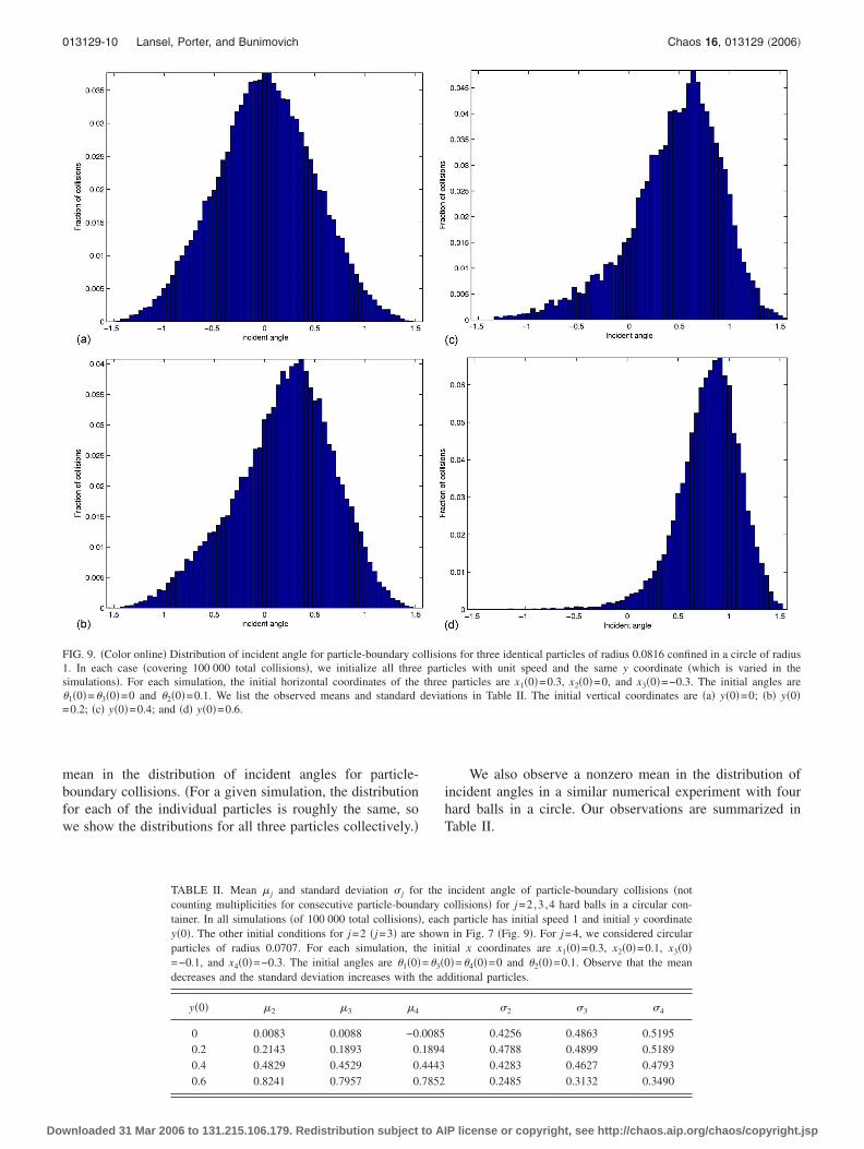
mean in the distribution of incident angles for particle-boundary collisions. �For a given simulation, the distributionfor each of the individual particles is roughly the same, sowe show the distributions for all three particles collectively.�

TABLE II. Mean � j and standard deviation � j forcounting multiplicities for consecutive particle-boundtainer. In all simulations �of 100 000 total collisions�y�0�. The other initial conditions for j=2 �j=3� are sparticles of radius 0.0707. For each simulation, th=−0.1, and x4�0�=−0.3. The initial angles are �1�0�decreases and the standard deviation increases with t

y�0� �2 �3 �4

0 0.0083 0.0088 −0.0.2 0.2143 0.1893 0.0.4 0.4829 0.4529 0.0.6 0.8241 0.7957 0.

FIG. 9. �Color online� Distribution of incident angle for particle-boundary co1. In each case �covering 100 000 total collisions�, we initialize all threesimulations�. For each simulation, the initial horizontal coordinates of the�1�0�=�3�0�=0 and �2�0�=0.1. We list the observed means and standard=0.2; �c� y�0�=0.4; and �d� y�0�=0.6.


We also observe a nonzero mean in the distribution ofincident angles in a similar numerical experiment with fourhard balls in a circle. Our observations are summarized inTable II.

incident angle of particle-boundary collisions �notollisions� for j=2,3 ,4 hard balls in a circular con-particle has initial speed 1 and initial y coordinatein Fig. 7 �Fig. 9�. For j=4, we considered circular

tial x coordinates are x1�0�=0.3, x2�0�=0.1, x3�0�0�=�4�0�=0 and �2�0�=0.1. Observe that the meanditional particles.

�2 �3 �4

0.4256 0.4863 0.51950.4788 0.4899 0.51890.4283 0.4627 0.47930.2485 0.3132 0.3490

ns for three identical particles of radius 0.0816 confined in a circle of radiusicles with unit speed and the same y coordinate �which is varied in the

particles are x1�0�=0.3, x2�0�=0, and x3�0�=−0.3. The initial angles aretions in Table II. The initial vertical coordinates are �a� y�0�=0; �b� y�0�

theary c

, eachhowne ini=�3�he ad

0085189444437852

llisiopart

threedevia



Dow

CONCLUSIONS

In this paper, we examined the dynamics of one-particleand few-particle billiards. These situations can be comparedin the context of noninteracting versus interacting hard ballsin a given container. �The “billiard limit” discussed in thepaper, in which the particle size becomes smaller, also pro-vides a means for comparison.� For example, two noninter-acting hard balls in a circular container are integrable, as thissystem just consists of two integrable billiards. However, weshowed using numerical simulations that two interactinghard balls in a circular container bear signatures of integra-bility even though the system is chaotic, and that its dynam-ics differs from that of two particles in a diamond container�which is chaotic even in the one-particle case�.

Consequently, we have shown that the shape of a con-tainer confining a system of interacting particles does matter,despite the fact that this aspect of the dynamics in the behav-ior of a gas of particles seems to be essentially neglected ininvestigations of these systems. In fact, the container shapemay be of comparable importance to that of the interactionpotential. Although the importance of the shape of the con-tainer �the so-called “billiard table”� for systems of noninter-acting particles is universally acknowledged, a “silent con-sensus” still exists that if the interaction potential isnontrivial, then a system of interacting particles must be er-godic in the thermodynamic limit. We have shown in thispaper, however, that this is not true for systems of a fewinteracting particles, which have thus far received little atten-tion. With the emergence of nanosystems and new experi-mental techniques, such systems are now among the mostimportant ones for various applications.19,24

Exactly solvable billiard systems demonstrating all threepossible types of behavior �integrability, chaos, and mixeddynamics� motivate natural container shapes to study the dy-namics of a few nontrivially interacting particles. While thefirst small step has been made in this paper, most of theproblems in this area remain completely open; we mention afew of them in passing. First, it is well-known in statisticalphysics that the high-density limit is more regular than thelow-density limit �where, for example, logarithmic terms ap-pear in the asymptotics of transport coefficients36�. We haveobserved this in our numerical studies as well. In fact, itseems to be a general phenomenon for which a theory shouldbe developed without the ubiquitous assumption that thenumber of particles is a large parameter. As usual, the tem-poral asymptotics of both correlation functions and Poincarérecurrences should be investigated in various situations, in-cluding all three types of behavior in billiards �noninteract-ing particles� and for broad classes of potentials. One of thekey questions is what happens to the relative volume ofKAM islands when the number of particles tends toinfinity.12 Again, the silent consensus �i.e., a belief withoutproofs or convincing demonstrations� is that this relative vol-ume tends to zero. However, it has been demonstrated thatthis is at least not always true.12 Hence, it is not at all un-likely that nonlinear dynamics will reveal some new sur-
prises in further investigations of this phenomenon.

ACKNOWLEDGMENTS

S.L. and M.A.P. acknowledge support provided by anNSF VIGRE grant awarded to the School of Mathematics atGeorgia Tech. The work of L.A.B. and S.L. was partiallysupported by NSF Grant No. DMS 0140165. L.A.B. alsoacknowledges the support of the Humboldt Foundation, S.L.acknowledges funding from a Georgia Tech PURA award,and M.A.P. acknowledges support from the Gordon andBetty Moore Foundation through Caltech’s Center for thePhysics of Information. We also thank Bill Casselman andNir Davidson for useful conversations and the anonymousreferee for suggestions that led to significant improvementsin the paper.

1V. I. Arnold, “Proof of A. N. Kolmogorov’s theorem on the preservation ofquasiperiodic motions under small perturbations of the Hamiltonian,”Russ. Math. Surveys 18, 9–36 �1963�.

2V. I. Arnold, “Small divisor problems in classical and celestial mechan-ics,” Russ. Math. Surveys 18, 85–192 �1963�.

3A. N. Kolmogorov, “On conservation of conditionally periodic motionsunder small perturbations of the Hamiltonian,” Dokl. Akad. Nauk SSSR98, 527–530 �1954�.

4J. Moser, “On invariant curves of area-preserving mappings of an annu-lus,” Nachr. Akad. Wiss. Goett. II, Math.-Phys. Kl. 2, 1–20 �1962�.

5D. V. Anosov and Ya. G. Sinai, “Some smooth ergodic systems,” Russ.Math. Surveys 22, 103–167 �1967�.

6Ya. G. Sinai, “On the foundation of the ergodic hypothesis for a dynamicalsystem of statistical mechanics,” Dokl. Akad. Nauk SSSR 153, 1261–1264 �1963�.

7S. Smale, “Differentiable dynamical systems,” Bull. Am. Math. Soc. 73,747–817 �1967�.

8M. V. Berry, “Regularity and chaos in classical mechanics, illustrated bythree deformations of a circular billiard,” Eur. J. Phys. 2, 91–102 �1981�.

9S. De Bièvre, P. E. Parris, and A. Silvius, “Chaotic dynamics of a freeparticle interacting linearly with a harmonic oscillator,” Physica D 208,96–114 �2005�.

10N. Saitô, H. Hirooka, J. Ford, F. Vivaldi, and G. H. Walker, “Numericalstudy of billiard motion in an annulus bounded by non-concentric circles,”Physica D 5, 273–286 �1982�.

11L. A. Bunimovich, “Mushrooms and other billiards with divided phasespace,” Chaos 11, 802–808 �2001�.

12L. A. Bunimovich, “Kinematics, equilibrium, and shape in Hamiltoniansystems: The ‘LAB’ effect,” Chaos 13, 903–912 �2003�.

13E. G. Altmann, A. E. Motter, and H. Kantz, “Stickiness in mushroombilliards,” Chaos 15, 033105 �2005�.

14A. Kudrolli, V. Kidambi, and S. Sridhar, “Experimental studies of chaosand localization in quantum wave functions,” Phys. Rev. Lett. 75, 822–825 �1995�.

15J. Stein and H. J. Stöckmann, “Experimental determination of billiardwave functions,” Phys. Rev. Lett. 68, 2867–2870 �1992�.

16H. J. Stöckmann and J. Stein, “Quantum chaos in billiards studied bymicrowave-absorption,” Phys. Rev. Lett. 64, 2215–2218 �1990�.

17C. M. Marcus, A. J. Rimberg, R. M. Westervelt, P. F. Hopkins, and A. C.Gossard, “Conductance fluctuations and chaotic scattering in ballistic mi-crostructures,” Phys. Rev. Lett. 69, 506–509 �1992�.

18M. F. Andersen, A. Kaplan, T. Grünzweig, and N. Davidson, “Decay ofquantum correlations in atom optics billiards with chaotic and mixed dy-namics,” e-print quant-ph/0404118.

19N. Friedman, A. Kaplan, D. Carasso, and N. Davidson, “Observation ofchaotic and regular dynamics in atom-optics billiards,” Phys. Rev. Lett.86, 1518–1521 �2001�.

20C. Zhang, J. Liu, M. G. Raizen, and Q. Niu, “Quantum chaos of Bogoliu-bov waves for a Bose-Einstein condensate in stadium billiards,” Phys.Rev. Lett. 93, 074101 �2004�.

21B. J. Alder and T. E. Wainwright, “Decay of velocity autocorrelation func-tion,” Phys. Rev. A 1, 18–21 �1970�.

22Ch. Dellago, H. A. Posch, and W. G. Hoover, “Lyapunov instability in asystem of hard disks in equilibrium and nonequilibrium steady states,”Phys. Rev. E 53, 1485–1501 �1996�.

23
H. A. Posch and R. Hirschl, “Simulations of billiards and of hard body


Dow

fluids,” in Hard Ball Systems and the Lorentz Gas, Vol. 101 of Encyclo-paedia of Mathematical Sciences, edited by D. Szász �Springer-Verlag,Berlin, Germany, 2000�, pp. 279–314.

24D. M. Harber, H. J. Lewandowski, J. M. McGuirk, and E. A. Cornell,“Effect of cold collisions on spin coherence and resonance shifts in amagnetically trapped ultracold gas,” Phys. Rev. A 66, 053616 �2002�.

25P. Cvitanović, R. Artuso, R. Mainieri, G. Tanner, and G. Vattay, Chaos:Classical and Quantum, 11th ed. �Niels Bohr Institute, Copenhagen,2005�; ChaosBook.org

26Ya. G. Sinai, “WHAT IS¼a billiard,” Not. Am. Math. Soc. 51, 412–413�2004�.

27A. Katok and B. Hasselblatt. Introduction to the Modern Theory of Dy-namical Systems �Cambridge University Press, New York, 1995�.

28Ya. G. Sinai, “Dynamical systems with elastic reflections,” Russ. Math.Surveys 25, 137–188 �1970�.

29P. Garrido and G. Gallavotti, “Billiards correlation functions,” J. Stat.Phys. 76, 549–586 �1994�.

30M. C. Gutzwiller, Chaos in Classical and Quantum Mechanics, No. 1 in


Interdisciplinary Applied Mathematics �Springer-Verlag, New York,1990�.

31S. W. MacDonald and A. N. Kaufman, “Spectrum and eigenfunctions fora Hamiltonian with stochastic trajectories,” Phys. Rev. Lett. 42, 1189–1191 �1979�.

32S. W. MacDonald and A. N. Kaufman, “Wave chaos in the stadium: Sta-tistical properties of short-wave solutions of the Helmholtz equation,”Phys. Rev. A 37, 3067–3086 �1988�.

33V. Lopac, I. Mrkonjic, N. Pavin, and D. Radic, “Chaotic dynamics of theelliptical stadium billiard in the full parameter space,” e-printnlin.CD/0507014.

34G. Del Magno and R. Markarian, “Bernoulli elliptical stadia,” Commun.Math. Phys. 233, 211–230 �2003�.

35S. Lansel and M. A. Porter, “A graphical user interface to simulate clas-sical billiard systems,” e-print nlin.CD/0405003.

36M. Résibois and M. De Leener, Classical Kinetic Theory of Fluids �JohnWiley and Sons, New York, 1977�.


One-particle and few-particle billiards - University of Oxford · One-particle and few-particle...

Documents

Transcript of One-particle and few-particle billiards - University of Oxford · One-particle and few-particle...