
ON TWO-DIMENSIONAL SPARSE MATRIX PARTITIONINGgraal.ens-lyon.fr/~bucar/papers/ucca2D.pdf · SIAM J....
28
SIAM J. SCI. COMPUT. c 2010 Society for Industrial and Applied Mathematics Vol. 32, No. 2, pp. 656–683 ON TWO-DIMENSIONAL SPARSE MATRIX PARTITIONING: MODELS, METHODS, AND A RECIPE ∗ ¨ UM ˙ IT V. C ¸ ATALY ¨ UREK † , CEVDET AYKANAT ‡ , AND BORA UC ¸ AR § Abstract. We consider two-dimensional partitioning of general sparse matrices for parallel sparse matrix-vector multiply operation. We present three hypergraph-partitioning-based methods, each having unique advantages. The first one treats the nonzeros of the matrix individually and hence produces fine-grain partitions. The other two produce coarser partitions, where one of them imposes a limit on the number of messages sent and received by a single processor, and the other trades that limit for a lower communication volume. We also present a thorough experimental evaluation of the proposed two-dimensional partitioning methods together with the hypergraph-based one-dimensional partitioning methods, using an extensive set of public domain matrices. Furthermore, for the users of these partitioning methods, we present a partitioning recipe that chooses one of the partitioning methods according to some matrix characteristics. Key words. sparse matrix partitioning, parallel matrix-vector multiplication, hypergraph par- titioning, two-dimensional partitioning, combinatorial scientific computing AMS subject classifications. 05C50, 05C65, 65F10, 65F50, 65Y05 DOI. 10.1137/080737770 1. Introduction. Sparse matrix-vector multiply operation forms the computa- tional core of many iterative methods including solvers for linear systems, linear pro- grams, eigensystems, and least squares problems. In these solvers, the computations y ← Ax are performed repeatedly with the same large, sparse, possibly unsymmetric or rectangular matrix A and with a changing input vector x. Our aim is to efficiently parallelize these multiply operations by two-dimensional (2D) partitioning of the ma- trix A in such a way that the computational load per processor is balanced and the communication overhead is low. Graph and hypergraph partitioning models have been used for one-dimensional (1D) partitioning of sparse matrices [4, 5, 8, 9, 19, 20, 25, 26, 30, 32, 37]. In these models, a K-way partition of the vertices of a given graph or hypergraph is computed. The partitioning constraint is to maintain a balance criterion on the number of vertices in each part; if the vertices are weighted, then the constraint is to maintain a balance criterion on the sum of the vertex weights in each part. The partitioning objective is to minimize the cutsize of the partition defined over the edges or hyperedges. The par- titioning constraint and objective relate, respectively to, maintaining a computational ∗ Received by the editors October 10, 2008; accepted for publication (in revised form) October 21, 2009; published electronically February 24, 2010. http://www.siam.org/journals/sisc/32-2/73777.html † Departments of Biomedical Informatics and Electrical & Computer Engineering, The Ohio State University, Columbus, OH 43210 ([email protected]). The work of this author is supported in part by the National Science Foundation grants CNS-0643969, OCI-0904809, OCI-0904802, and CNS-0403342, and the U.S. DOE SciDAC Institute grant DE-FC02-06ER2775. ‡ Computer Engineering Department, Bilkent University, Ankara, Turkey ([email protected]. edu.tr). The work of this author is partially supported by The Scientific and Technical Research Council of Turkey (T ¨ UB ˙ ITAK) under project EEEAG-109E019. § Centre National de la Recherche Scientifique, Laboratoire de l’Informatique du Parall´ elisme, (UMR CNRS -ENS Lyon-INRIA-UCBL), Universit´ e de Lyon, 46, all´ ee d’Italie, ENS Lyon, F-69364, Lyon Cedex 7, France ([email protected]). The work of this author is partially supported by Agence Nationale de la Recherche through SOLSTICE project ANR-06-CIS6-010. 656
Transcript of ON TWO-DIMENSIONAL SPARSE MATRIX PARTITIONINGgraal.ens-lyon.fr/~bucar/papers/ucca2D.pdf · SIAM J....

SIAM J. SCI. COMPUT. c© 2010 Society for Industrial and Applied MathematicsVol. 32, No. 2, pp. 656–683
ON TWO-DIMENSIONAL SPARSE MATRIX PARTITIONING:MODELS, METHODS, AND A RECIPE∗
UMIT V. CATALYUREK† , CEVDET AYKANAT‡, AND BORA UCAR§
Abstract. We consider two-dimensional partitioning of general sparse matrices for parallelsparse matrix-vector multiply operation. We present three hypergraph-partitioning-based methods,each having unique advantages. The first one treats the nonzeros of the matrix individually and henceproduces fine-grain partitions. The other two produce coarser partitions, where one of them imposesa limit on the number of messages sent and received by a single processor, and the other trades thatlimit for a lower communication volume. We also present a thorough experimental evaluation of theproposed two-dimensional partitioning methods together with the hypergraph-based one-dimensionalpartitioning methods, using an extensive set of public domain matrices. Furthermore, for the usersof these partitioning methods, we present a partitioning recipe that chooses one of the partitioningmethods according to some matrix characteristics.
Key words. sparse matrix partitioning, parallel matrix-vector multiplication, hypergraph par-titioning, two-dimensional partitioning, combinatorial scientific computing
AMS subject classifications. 05C50, 05C65, 65F10, 65F50, 65Y05
DOI. 10.1137/080737770
1. Introduction. Sparse matrix-vector multiply operation forms the computa-tional core of many iterative methods including solvers for linear systems, linear pro-grams, eigensystems, and least squares problems. In these solvers, the computationsy← Ax are performed repeatedly with the same large, sparse, possibly unsymmetricor rectangular matrix A and with a changing input vector x. Our aim is to efficientlyparallelize these multiply operations by two-dimensional (2D) partitioning of the ma-trix A in such a way that the computational load per processor is balanced and thecommunication overhead is low.
Graph and hypergraph partitioning models have been used for one-dimensional(1D) partitioning of sparse matrices [4, 5, 8, 9, 19, 20, 25, 26, 30, 32, 37]. In thesemodels, a K-way partition of the vertices of a given graph or hypergraph is computed.The partitioning constraint is to maintain a balance criterion on the number of verticesin each part; if the vertices are weighted, then the constraint is to maintain a balancecriterion on the sum of the vertex weights in each part. The partitioning objective isto minimize the cutsize of the partition defined over the edges or hyperedges. The par-titioning constraint and objective relate, respectively to, maintaining a computational
∗Received by the editors October 10, 2008; accepted for publication (in revised form) October 21,2009; published electronically February 24, 2010.
http://www.siam.org/journals/sisc/32-2/73777.html†Departments of Biomedical Informatics and Electrical & Computer Engineering, The Ohio State
University, Columbus, OH 43210 ([email protected]). The work of this author is supportedin part by the National Science Foundation grants CNS-0643969, OCI-0904809, OCI-0904802, andCNS-0403342, and the U.S. DOE SciDAC Institute grant DE-FC02-06ER2775.
‡Computer Engineering Department, Bilkent University, Ankara, Turkey ([email protected]). The work of this author is partially supported by The Scientific and Technical ResearchCouncil of Turkey (TUBITAK) under project EEEAG-109E019.
§Centre National de la Recherche Scientifique, Laboratoire de l’Informatique du Parallelisme,(UMR CNRS -ENS Lyon-INRIA-UCBL), Universite de Lyon, 46, allee d’Italie, ENS Lyon, F-69364,Lyon Cedex 7, France ([email protected]). The work of this author is partially supported byAgence Nationale de la Recherche through SOLSTICE project ANR-06-CIS6-010.
656

ON TWO-DIMENSIONAL SPARSE MATRIX PARTITIONING 657
load balance and minimizing the total communication volume. The limitations of thegraph model have been shown in [8, 9, 19]. First, it tries to minimize a wrong objectivefunction, since edge-cut metric is only an approximation to the total communicationvolume. Second, it can only model square matrices. Alternative models such as bi-partite graph model [21], multi-constraint and multi-objective partitionings [43, 44],skewed partitioning [23], and those based on hypergraph partitioning [8, 9] have beenproposed. All these new models address some of the limitations of the standard model,but only in hypergraph-partitioning based ones, the partitioning objective is an exactmeasure of the total communication volume.
Earlier works on 2D matrix partitioning [22, 34, 35, 39] are based on checkerboardpartitioning. These works are typically suited to dense matrices or sparse matriceswith structured nonzero patterns that are difficult to exploit. Later works [7, 11, 12,52] are specifically targeted to sparse matrices. These works are based on differenthypergraph models and produce matrix partitionings with differing characteristics.These 2D partitioning models, as hypergraph-partitioning based models for 1D parti-tioning, encode the total communication volume exactly with the partitioning objec-tive. The hypergraph model in [11] is used to partition the matrices on nonzero basis.In other words, it produces fine-grain partitionings in which assignment decisions aremade in nonzero basis. The hypergraph model in [12] is used to obtain checkerboardpartitionings. In other words, the matrix is divided into blocks, and the blocks areassigned to processors. The partitioned matrix maps naturally onto a 2D mesh ofprocessors. Therefore, the communication along a matrix row or column is confinedto a subset of processors, and hence the total number of messages is limited. Theapproach presented in [52] applies recursive bisection in which each step partitionsthe current submatrix along the rows or columns using the hypergraph models for 1Dpartitioning. This approach does not limit the total number of messages.
In order to parallelize the matrix-vector multiply y ← Ax, we have to partitionthe vectors x and y as well. There are two alternatives in partitioning the vectors xand y. The first one, symmetric partitioning, is to have the same partition on x andy. The second one, nonsymmetric partitioning, is to have different partitions on x andy. There are three groups of methods to obtain vector partitionings. The methodsin the first group perform the vector partitioning implicitly using the partitions onthe matrix for symmetric partitioning [9, 11, 12]. The methods in the second groupperform the vector partitioning in an additional stage after partitioning the matrixfor nonsymmetric [3, 46, 47, 52] and symmetric [46, 52] partitionings. The methodsin the third group [50] enhance the previously proposed hypergraph models in orderto obtain vector and matrix partitionings simultaneously both for the symmetric andnonsymmetric partitioning cases. A common goal pursued by all these techniques isto assign a vector entry to a processor that has nonzeros in the corresponding row orcolumn of the matrix. In this paper, we are only interested in matrix partitioning,and we do not make use of any of those vector partitioning methods. However, weuse a simple vector partitioning method achieving the common goal stated above.
We present some background material on parallel matrix-vector multiply opera-tion based on 2D matrix partitioning, hypergraph partitioning, and hypergraph mod-els for 1D matrix partitioning in the next section. Section 3 presents three meth-ods with different assignment granularity and communication patterns for 2D matrixpartitioning: fine-grain, jagged-like, and checkerboard-like partitioning methods. Thefine-grain and the checkerboard-like models were briefly discussed, respectively, in [11]and [12]. The jagged-like partitioning model was only described in the first author’sthesis [7]. Section 4 contains further investigations on partitioning methods, including

658 UMIT V. CATALYUREK, CEVDET AYKANAT, AND BORA UCAR
a recipe on matrix partitioning alternatives. In section 5, we present experimentalresults.
Our contributions in this paper are fourfold: first, to present the jagged-likemethod for the first time, and the fine-grain and checkerboard-like methods in a moreaccessible venue (section 3); second, to investigate the merits of these three partition-ing approaches with respect to each other (section 4.1); third, to propose a recipe(section 4.4) which suggests a partitioning method among the existing 1D and theproposed 2D partitioning methods based on some easily computable matrix charac-teristics; fourth, a thorough and conclusive experimental evaluation (section 5) of the1D and 2D partitioning methods as well as the effectiveness of the proposed recipe.We also discuss (sections 4.2 and 4.3) how communication requirements can be mod-eled when collective communication primitives are used in the matrix-vector multiplyoperations and characterize a class of applications whose efficient parallelization canbe obtained by using hypergraph partitioning models.
2. Preliminaries. Here, we give an overview of algorithms for parallel matrix-vector multiplies, hypergraph partitioning problem and its variations, and remind thereader of the hypergraph models for 1D sparse matrix partitioning.
2.1. Row-column-parallel matrix-vector multiply. Consider the computa-tions y← Ax, where the nonzeros of the M ×N matrix A are partitioned arbitrarilyamong K processors such that each processor Pk owns a mutually disjoint subset ofnonzeros, A(k). Then, A can be written as A =
∑k A
(k). The vectors y and x arealso partitioned among processors, where the processor Pk holds x(k), a dense vectorof size Nk, and it is responsible for computing y(k), a dense vector of sizeMk. We notethat the vectors x(k) for k = 1, . . . ,K are disjoint and hence
∑k Nk = N ; similarly
the vectors y(k) for k = 1, . . . ,K are disjoint and hence∑
k Mk = M . In this setting,the sparse matrix A(k) owned by processor Pk can be permuted and written as
(2.1) A(k) =
⎡⎢⎢⎢⎢⎢⎢⎢⎣
A(k)11 · · · A
(k)1� · · · A
(k)1K
.... . .
.... . .
...
A(k)�1 · · · A
(k)�� · · · A
(k)�K
.... . .
.... . .
...
A(k)K1 · · · A
(k)K� · · · A
(k)KK
⎤⎥⎥⎥⎥⎥⎥⎥⎦.
Here, the blocks in the row-block stripe A(k)k∗ = {A(k)
k1 , . . . ,A(k)kk , . . . ,A
(k)kK} have
row dimension of Mk, and similarly the blocks in the column-block stripe A(k)∗k =
{A(k)1k , . . . ,A
(k)kk ,. . . ,A
(k)Kk} have column dimension of Nk. The x-vector entries that
are needed by processor Pk are represented as x(k) = [x(k)1 , . . . , x
(k)k , . . . , x
(k)K ], a sparse
column vector (we omit the transpose sign for column vectors for simplicity in the
notation), where x(k)� contains only those entries of x(�) of processor P� corresponding
to the nonzero columns in A(k)∗� . Here, the vector x
(k)k is equivalent to x(k), defined ac-
cording to the given partition on the x-vector (hence the vector x(k) is of size at leastNk). The y-vector entries for which the processor Pk computes partial results are rep-
resented as a sparse vector y(k) = [y(1)k , . . . , y
(k)k , . . . , y
(K)k ], where y
(�)k contains only
the partial results for y(�) corresponding to the nonzero rows in A(k)�∗ . Since the paral-
lelism is achieved on a nonzero basis, we derive a nonzero-based sparse matrix-vectormultiply (SpMxV) algorithm. This algorithm, which we call the row-column-parallelalgorithm, executes at each processor Pk the steps that follow.

ON TWO-DIMENSIONAL SPARSE MATRIX PARTITIONING 659
1 2 3 4 5 6 7 8 9 10 11 12 13 14 15 16
1
2
3
4
5
6
7
8
9
10
11
12
13
14
15
16
nnz = 47
(a)
= X
y A x
4 8 12 16 3 6 11 14 2 7 9 15 1 5 10 13
4
8
12
16
3
6
11
14
2
7
9
15
1
5
10
13
nnz = 47vol = 7 imbal = [ 14.9%, 10.6%]
4
8
12
16
3
6
11
14
2
7
9
15
1
5
10
13
4
8
12
16
3
6
11
14
2
7
9
15
1
5
10
13
(b)
Fig. 2.1. (a) A 16×16 unsymmetric matrix A with nnz = 47 nonzeros. (b) Sparse matrix-vectormultiplication y ← Ax of the sample matrix A. The matrix and the input and output vectors arepartitioned among four processors. The four disjoint sets of nonzeros and vector entries that areassigned to the four processors are shown with four distinct shapes and colors. The average numberof nonzeros per processor is 47/4 = 11.75. The maximum number of nonzeros of a processor is 13,giving an imbalance ratio of 10.6%; i.e., the maximally loaded processor has 10.6% more nonzerosthan the average number of nonzeros. The minimum number of nonzeros of a processor is 10, being14.9% less than the average number of nonzeros. We indicate the imbalance among the parts, imbal,using these two marginal percentages. The total communication volume is denoted with vol.
1. For each � �= k, form and send sparse vector x(�)k to processor P�, where x
(�)k
contains only those entries of x(k) corresponding to the nonzero columns in
A(�)∗k .
2. In order to form x(k) = [x(k)1 , . . . , x
(k)k , . . . , x
(k)K ], first define x
(k)k = x(k).
Then, for each � �= k whereA(k)∗� contains nonzeros, receive x
(k)� from processor
P�, corresponding to the nonzero columns in A(k)∗� .
3. Compute y(k) ← A(k)x(k).
4. For each � �= k, send the sparse partial-results vector y(�)k to processor P�,
where y(�)k contains only those partial results for y(�) corresponding to the
nonzero rows in A(k)�∗ .
5. Receive the partial-results vector y(k)� from each processor P� which has com-
puted a partial result for y(k), i.e., from each processor P� where A(�)k∗ has
nonzeros.6. Compute y(k) ← ∑
� y(k)� , adding all the partial-results y
(k)� received in the
previous step to its own partial results for y(k).There are two communication phases in this algorithm. The first one is just
before the local matrix-vector multiply, and it is due to the communication of thex-vector entries (steps 1 and 2). We refer to this operation as expand. The secondcommunication phase is just after the local matrix-vector multiply, and it is due tothe communication of the partial results on y-vector entries (steps 4 and 5). We referto this operation as fold. It is possible to restructure this algorithm in order to takefull advantage of communication and computation overlap [48].
Figure 2.1 shows a sample matrix and input- and output-vectors of a matrix-vector multiply operation, partitioned among four processors. The matrix is permuted

660 UMIT V. CATALYUREK, CEVDET AYKANAT, AND BORA UCAR
such that the rows and the columns of the matrix are aligned conformably with thepartition on the output- and input-vectors, respectively. The disjoint sets of nonzerosA(1) to A(4) are assigned to the processors P1 to P4 and each such set is shown witha distinct symbol in the figure. Processor P1 holds the (red) squares; processor P2
holds the (green) triangles; processor P3 holds the (blue) circles; and processor P4
holds the (magenta) diamonds. The number of nonzeros of the four processors are,respectively, 12, 12, 13, and 10. The average number of nonzeros is 47/4 = 11.75,the maximum is 13, being 10.6% more than the average, and the minimum is 10,being 14.9% less than the average. Consider the processor P1, to see the steps of themultiply algorithm and the communication operations performed by P1. Among all
blocks of A(1), only three are nonempty: A(1)11 , containing the nine nonzeros of the
(1, 1)-block in the figure; A(1)21 , containing the two nonzeros of the (2, 1)-block in the
figure; and A(1)13 containing the one nonzero of the (1, 3)-block. Processor P1 holds the
vector x(1) = [x4, x8, x12, x16] and has to compute the final result of the multiplication
for y(1) = [y4, y8, y12, y16]. It needs the x-vector entries x(1) = [x(1)1 , x
(1)3 ], where
x(1)1 = x(1) and x
(1)3 contain only those entries of x(3) of processor P3 corresponding
to the nonzero columns in A(3)∗3 , i.e., x
(1)3 = [x2]. During the course of the multiply
operation, P1 sends x(3)1 = [x12] to processor P3 in step 1; receives x
(1)3 = [x2] from
P3 to form x(1) in step 2; performs the multiplication operations in step 3; sends the
partial-result vector y(2)1 for y14 to processor P2 in step 4; receives partial result for
y4 from processor P2 in step 5; and finally adds up the partial result received in theprevious step to its own results to compute y(1) = [y4, y8, y12, y16].
It is implicit in the algorithm that row coherence and column coherence are im-portant factors in a matrix partition for parallel SpMxV. Column coherence relatesto the fact that nonzeros on the same column require the same x-vector entry. Rowcoherence relates to the fact that nonzeros on the same row generate partial resultsfor the same y-vector entry. In a partitioning, disturbing column coherence incursexpand communication of x-vector entries, and disturbing row coherence incurs foldcommunication of partial y-vector results.
If the sparsity structure ofA is ignored, in the worst case, the total communicationvolume of the nonzero-based parallel matrix-vector multiply algorithm is (K − 1)N +(K − 1)M units, and the total number of messages is 2K(K − 1). The worst caseoccurs when there is at least one nonzero in every single row and every single columnof A(k) for all k. By restricting the partitioning of nonzeros to 1D, i.e., partitioning
such that only row-block stripe A(k)k∗ (or column-block stripe A
(k)∗k ) would have all
of the nonzeros in A(k), one can reduce the worst-case communication requirementsto K(K − 1) messages with a total volume of (K − 1)N , or (K − 1)M units. Byfurther restricting the partitioning such that only a subset of blocks in row-block
stripe A(k)k∗ and column-block stripe A
(k)∗k have nonzeros, it is also possible to achieve
a 2D distribution [22, 34, 35, 39], called transpose-free blocked 2D partitioning, thatwould reduce the worst-case communication requirements to 2K(
√K − 1) messages
with a total volume of (√K − 1)N + (
√K − 1)M units.
2.2. Hypergraph partitioning. A hypergraph H=(V ,N ) is defined as a setof vertices V and a set of nets (hyperedges) N . Every net nj ∈ N is a subset ofvertices, i.e., nj⊆V . The vertices in a net nj are called its pins . The number of pinsof a net defines its size. Weights can be associated with the vertices. We use wi todenote the weight of the vertex vi.
ON TWO-DIMENSIONAL SPARSE MATRIX PARTITIONING 661
V 3
V 1
n4
n7
n5
n6
n2
n3n1
n8
n9
u1 u2
u3
u5
u7u6
u9
u10
V 2
u8
u4
u11
u12
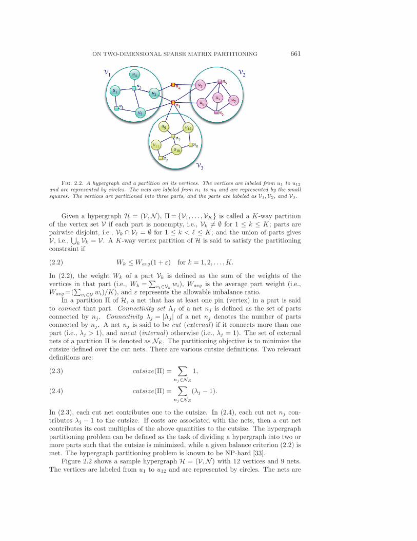
Fig. 2.2. A hypergraph and a partition on its vertices. The vertices are labeled from u1 to u12
and are represented by circles. The nets are labeled from n1 to n9 and are represented by the smallsquares. The vertices are partitioned into three parts, and the parts are labeled as V1,V2, and V3.
Given a hypergraph H = (V ,N ), Π = {V1, . . . ,VK} is called a K-way partitionof the vertex set V if each part is nonempty, i.e., Vk �= ∅ for 1 ≤ k ≤ K; parts arepairwise disjoint, i.e., Vk ∩ V� = ∅ for 1 ≤ k < � ≤ K; and the union of parts givesV , i.e., ⋃k Vk = V . A K-way vertex partition of H is said to satisfy the partitioningconstraint if
(2.2) Wk ≤Wavg(1 + ε) for k = 1, 2, . . . ,K.
In (2.2), the weight Wk of a part Vk is defined as the sum of the weights of thevertices in that part (i.e., Wk =
∑vi∈Vk
wi), Wavg is the average part weight (i.e.,Wavg =(
∑vi∈V wi)/K), and ε represents the allowable imbalance ratio.
In a partition Π of H, a net that has at least one pin (vertex) in a part is saidto connect that part. Connectivity set Λj of a net nj is defined as the set of partsconnected by nj. Connectivity λj = |Λj | of a net nj denotes the number of partsconnected by nj. A net nj is said to be cut (external) if it connects more than onepart (i.e., λj > 1), and uncut (internal) otherwise (i.e., λj = 1). The set of externalnets of a partition Π is denoted as NE . The partitioning objective is to minimize thecutsize defined over the cut nets. There are various cutsize definitions. Two relevantdefinitions are:
cutsize(Π) =∑
nj∈NE
1,(2.3)
cutsize(Π) =∑
nj∈NE
(λj − 1).(2.4)
In (2.3), each cut net contributes one to the cutsize. In (2.4), each cut net nj con-tributes λj − 1 to the cutsize. If costs are associated with the nets, then a cut netcontributes its cost multiples of the above quantities to the cutsize. The hypergraphpartitioning problem can be defined as the task of dividing a hypergraph into two ormore parts such that the cutsize is minimized, while a given balance criterion (2.2) ismet. The hypergraph partitioning problem is known to be NP-hard [33].
Figure 2.2 shows a sample hypergraph H = (V ,N ) with 12 vertices and 9 nets.The vertices are labeled from u1 to u12 and are represented by circles. The nets are

662 UMIT V. CATALYUREK, CEVDET AYKANAT, AND BORA UCAR
labeled from n1 to n9 and are represented by the small squares. The pins are shownwith lines. For example, net n2 contains vertices u1 to u4. The vertices are partitionedinto three parts, each shown by a large cycle encompassing the vertices in that partand labeled as V1,V2, and V3. The nets n1 and n4 connect, respectively, three andtwo parts, and hence they are in the cut: the other nets are internal to a part. Thecutsize according to (2.3) is 2, as there are two nets in the cut, whereas the cutsizeaccording to (2.4) is 3, where n1 and n4 contribute, respectively, 2 and 1. Assumingvertices of unit weights, the partition has a perfect balance.
A recent variant of the above problem is the multi-constraint hypergraph parti-tioning [1, 7, 12, 27, 44] in which each vertex has a vector of weights associated withit. The partitioning objective is the same as above, and the partitioning constraintis to satisfy a balancing constraint associated with each weight. We use the notationwi,g to denote the G weights of a vertex vi for g = 1, . . . , G. Hence, the balancecriterion (2.2) can be rewritten as
(2.5) Wk,g ≤Wavg,g (1 + ε) for k = 1, . . . ,K and g = 1, . . . , G,
where the gth weight Wk,g of a part Vk is defined as the sum of the gth weights of thevertices in that part (i.e., Wk,g=
∑vi∈Vk
wi,g), and Wavg,g is the average part weightfor the gth weight (i.e., Wavg,g = (
∑vi∈V wi,g)/K), and ε again represents allowed
imbalance ratio.
2.3. Hypergraph models for 1D sparse matrix partitioning. In the col-umn-net hypergraph model [8, 9] HR =(VR,NC) of matrix A, there exist one vertexvi ∈ VR and one net nj ∈ NC for each row ri and column cj , respectively. Netnj ⊆ VR contains the vertices corresponding to the rows that have a nonzero entry incolumn cj . That is, vi ∈ nj if and only if aij �= 0. Weight wi of a vertex vi ∈ VR is setto the total number of nonzeros in row ri. This model is used for rowwise partitioning.
In the row-net hypergraph model [8, 9] HC=(VC ,NR) of matrix A, there exist onevertex vj ∈ VC and one net ni ∈ NR for each column cj and row ri, respectively. Netni⊆VC contains the vertices corresponding to the columns that have a nonzero entryin row ri. That is, vj ∈ ni if and only if aij �= 0. Weight wj of a vertex vj ∈ VR isset to the total number of nonzeros in column cj . This model is used for columnwisepartitioning.
The use of the hypergraphs HR and HC in 1D sparse matrix partitioning for par-allelization of matrix-vector multiply operation is described in [8, 9]. In particular, ithas been shown that the partitioning objective of minimizing the cutsize (2.4) corre-sponds exactly to minimizing the total communication volume, and the partitioningconstraint of maintaining balance on part weights (2.2) corresponds to maintaining acomputational load balance for a given number K of processors.
3. Models and methods for 2D matrix partitioning. Here, we proposethree hypergraph-partitioning based methods for 2D sparse matrix partitioning forparallel y ← Ax computations. These three methods produce nonzero-to-processorassignments, i.e., map(aij) = Pk if aij is assigned to processor Pk. They do notaddress the vector partitioning problem. However, they rely on vector partitionsbeing consistent with the matrix partitions; consistent in the sense that each vectorentry xj or yi will be assigned to a processor having at least one nonzero in thecorresponding column (the jth column) or row (the ith row), respectively, of A. Ifthe vector partitioning is consistent, then the cutsize (2.4) in the proposed hypergraph-partitioning based models will be equivalent to the total communication volume. The

ON TWO-DIMENSIONAL SPARSE MATRIX PARTITIONING 663
vih
vii
vik
mivij
vjj
vlj
nj
Fig. 3.1. Dependency relation of 2D fine-grain hypergraph model.
consistency is easy to achieve for the nonsymmetric vector partitioning; xj can beassigned to any of the processors in {map(aij) : 1 ≤ i ≤ M and aij �= 0}, and yican be assigned to any of the processors in {map(aij) : 1 ≤ j ≤ N and aij �= 0}. Ifa symmetric partitioning is sought, then special care must be taken to assign a pairof matching input- and output-vector entries, e.g., xi and yi, to a processor havingnonzeros in the corresponding row and column. In order to have such a processor forall vector entry pairs, the sparsity pattern of the matrix A can be modified to have azero-free diagonal. In such cases, a consistent vector partition is guaranteed to exist,because the processors that own the diagonal entries can also own the correspondinginput- and output-vector entries; xi and yi can be assigned to map(aii). Therefore,throughout this section, we assume that a consistent vector partitioning is alwayspossible after partitioning the matrix A.
3.1. Fine-grain model and partitioning method. In the fine-grain model,an M × N matrix A with Z nonzeros is represented as a unit-weight hypergraphHZ =(VZ ,NRC) with |VZ | = Z vertices and |NRC | = M +N nets for 2D partitioning.There exists one vertex vij ∈ VZ corresponding to each nonzero aij in matrix A.For each row and for each column there exists a net in NRC . Let NRC = NR ∪ NCsuch that NR = {r1, . . . , rM} represents the set of nets corresponding to the rows,and NC = {c1, . . . , cN} represents the set of nets corresponding to the columns ofthe matrix A. The net ri contains the vertices corresponding to the nonzeros inthe ith row, and the net cj contains the vertices corresponding to the nonzeros inthe jth column. That is, vij ∈ ri and vij ∈ cj if and only if aij �= 0. Note thateach vertex vij is a pin of exactly two nets. Each vertex vij corresponds to the
scalar multiply operation yji = aijxj . Therefore, each column-net cj represents theset of scalar multiply operations that need xj during the expand phase, and eachrow-net ri represents the set of scalar multiply results needed to accumulate yi inthe fold phase. Each vertex vij has unit computational weight wij = 1. Figure 3.1illustrates the dependency relation view of the 2D fine-grain model. As seen in thisfigure, column-net cj = {vij , vjj , vlj} of size 3 represents the three scalar multiply
operations yji =aijxj , yjj =ajjxj , and yjl =aljxj which need xj . In this figure, row-net
ri = {vih, vii, vik, vij} of size 4 represents the four scalar multiply results yhi = aihxh,
yii=aiixi,yki =aikxk andyji =aijxj which are needed to accumulate yi=yhi+yii+y
ki+y
ji .
The fine-grain partitioning method partitions the hypergraph HZ given above.Consider a partition Π={V1, . . . ,VK} of the vertices of HZ . Without loss of general-ity, we assign part Vk to processor Pk for k=1, . . . ,K. That is, for each k = 1, . . . ,Kwe set map(aij) = Pk for all vij ∈ Vk. Since Π satisfies the balance constraint (2.2),it achieves a computational load balance among processors under the vertex weightdefinition given above. Consider an x-vector entry xj needed by only one processor.

664 UMIT V. CATALYUREK, CEVDET AYKANAT, AND BORA UCAR
Then all of the nonzeros in column j should have been assigned to a single processor.This implies that the column-net cj connects only one part. Hence the contributionof that net to the cutsize is zero. Consider an x-vector entry xj needed by more thanone, say p, processors. Then the nonzeros in column j should have been partitionedamong these p processors. This implies that the column-net cj connects p parts. Thatis, λj = p holds. The contribution of this net to the cutsize is equal to p− 1. Due tothe consistency of the vector partitioning, xj is assigned to one of those p processors.Therefore, we have the equivalence between λj − 1 and the communication volumeregarding xj . Similar arguments hold for the y-vector entries, since the sets NR andNC are disjoint.
Note that the nonzeros in the same row or column are treated independentlyby the fine-grain partitioning method. Therefore, neither row coherence nor columncoherence is respected.
3.2. Jagged-like partitioning method. Jagged partitioning has been succes-sively used in partitioning 2D spatial computational domains (2D workload arrays)for load balancing in the parallelization of several irregular computations includingSpMxV computations on processor meshes [31, 38, 40, 41, 42]. In this method, fora P × Q processor mesh, the matrix is first partitioned into P horizontal (vertical)strips and every horizontal (vertical) strip is independently partitioned into Q sub-matrices. That is, splits span the entire array/matrix in one dimension, while theyare jagged in the other dimension. Asymptotically and run-time efficient exact algo-rithms are proposed and implemented for producing jagged partitions with optimalbalance [31, 36, 40]. However, the jagged partitioning methods adopted in sparse ma-trix partitioning unnecessarily restrict the search space since they do not utilize theflexibility of disturbing the integrity and original ordering of the rows/columns of thematrices, and furthermore, they do not consider the minimization of communicationvolume explicitly.
The proposed jagged-like partitioning method uses the row-net and column-nethypergraph models proposed in [8, 9]. The proposed partitioning method is a two-step method, in which each step models either the expand phase or the fold phase ofthe parallel SpMxV algorithm. Therefore, we have two alternative schemes for thispartitioning method. We present the one which models the expands in the first stepand the folds in the second step. A similar discussion holds for the other scheme.
Given an M × N matrix A and the number K of processors organized as aP × Q mesh, the jagged-like partitioning model proceeds as shown in Figure 3.2.The algorithm has two main steps. First, A is partitioned rowwise into P partsusing the column-net hypergraph model HR discussed in section 2.3 (lines 1 and 2 ofFigure 3.2). Consider a P -way partition ΠR ofHR. From the partition ΠR, we obtainP submatrices Ap for p = 1, . . . , P each having roughly equal number of nonzeros.For each p, the rows of the submatrix Ap correspond to the vertices in Rp. Hence,Ap is of size Mp ×N , where Mp = |Rp| (lines 6 and 7 of Figure 3.2). We assign thesubmatrix Ap to the pth row of the processor mesh. Second, each submatrix Ap for1 ≤ p ≤ P is independently partitioned columnwise into Q parts using the row-nethypergraph Hp (lines 8 and 9 of Figure 3.2). Observe that the nonzeros in the ithrow of A are partitioned among the Q processors in a row of the processor mesh. Inparticular, if vi ∈ Rp at the end of line 2 of the algorithm, then the nonzeros in theith row of A are partitioned among the processors in the pth row of the processormesh. After partitioning the submatrix Ap columnwise, we fill the map array for thenonzeros residing in Ap.

ON TWO-DIMENSIONAL SPARSE MATRIX PARTITIONING 665
Jagged-Like-Partitioning(A,K = P ×Q, ε1, ε2)Input: a matrix A, the number of processors K = P ×Q, and the imbalance ratios ε1, ε2.Output: map(aij) for all aij �= 0 and totalVolume.
1: HR = (VR,NC)← columnNet(A)2: ΠR = {R1, . . . ,RP } ← partition(HR, P, ε1) � rowwise partitioning of A3: expandVolume← cutsize(ΠR)4: foldVolume← 05: for p = 1 to P do6: Rp = {ri : vi ∈ Rp}7: Ap ← A(Rp, :) � submatrix indexed by rows Rp
8: Hp = (Vp,Np)← rowNet(Ap)9: ΠC
p = {C1p, . . . , CQp } ← partition(Hp, Q, ε2) � columnwise partitioning of Ap
10: foldVolume←foldVolume +cutsize(ΠCp)
11: for all aij �= 0 of Ap do12: map(aij) = Pp,q ⇔ cj ∈ Cqp13: return totalVolume←expandVolume+foldVolume
Fig. 3.2. Jagged-like partitioning.
Consider processor loads obtained according to the map array at the end of thealgorithm. The Q processors in a row of the processor mesh are assigned a roughly
equal number of nonzeros, i.e., each having at most (1+ε2)nnz (Ap)
Q nonzeros, due to the
balance constraint (2.2) met while partitioning Hp. Furthermore, we have nnz(Ap) ≤(1 + ε1)
nnz (A)P for all p, due to the balance constraint met while partitioning HR.
Therefore, a processor can get as many as (1 + ε1 + ε2 + ε1ε2)nnz (A)
K nonzeros. Inother words, the resulting K-way partitioning of A is guaranteed to satisfy a balanceconstraint with an imbalance ratio of ε = (ε1 + ε2 + ε1ε2).
Consider a y-vector entry yi. As noted above, the nonzeros in the row ri arepartitioned in the columnwise partitioning of the submatrix Ap containing ri (line 9of the algorithm). Hence, the processors that contribute to yi exactly correspond tothe parts in the connectivity set of the row-net ri in Hp. That is, the volume ofcommunication required to fold yi is accurately represented as a part of “foldVolume”in the algorithm. Consider an x-vector entry xj . Suppose it is needed by q processors.Then, the nonzeros in the jth column of A should have been partitioned amongthose q processors. Note that due to the row-net model representing the columns asvertices, the nonzeros of the jth column in a submatrix Ap are assigned to exactly oneprocessor. In other words, the jth column of A should have nonzeros in q submatricesafter the rowwise partitioning in line 2 of the algorithm. Therefore, the connectivityof the net nj ∈ NC should be q. Due to the consistency of the vector partitioning,the volume of communication regarding xj is equal to (q − 1) = (λj − 1). Therefore,the volume of communication regarding xj is accurately represented as a part of“expandVolume” in the algorithm.
As an example run of the algorithm, consider the 16 × 16 matrix shown in Fig-ure 2.1 to be partitioned among the processors of a 2×2 mesh. Figure 3.3(a) illustratesthe column-net representation of the sample matrix. For simplicity of presentation,we labeled the vertices and the nets of the hypergraphs with letters “r” and “c” todenote the rows and columns of the matrix. We first partition the matrix rowwise intotwo parts, and assign each part to a row of the processor mesh, namely, to processors{P1, P2} and {P3, P4}. The resulting permuted matrix is displayed in Figure 3.3(b).

666 UMIT V. CATALYUREK, CEVDET AYKANAT, AND BORA UCAR
R2
r1
R1r2
r3
r4
r5
r6
r7
r8
r9
r10
r11
r12 r13
r14r15
r16
c1
c2
c3
c4
c5
c6
c7
c8
c9
c10
c11
c12
c13c14
c15
c16
(a)
3 4 6 8 11 12 14 16 1 2 5 7 9 10 13 15
3
4
6
8
11
12
14
16
1
2
5
7
9
10
13
15
nnz = 47vol = 3 imbal = [ 2.1%, 2.1%]
(b)
Fig. 3.3. First step of 4-way jagged-like partitioning of the matrix shown in Figure 2.1: (a)2-way partitioning ΠR of column-net hypergraph representation HR of A; (b) 2-way rowwise par-titioning of matrix AΠ obtained by permuting A according to the partitioning induced by Π; thenonzeros in the same partition are shown with the same shape and color; the deviation of the min-imum and maximum numbers of nonzeros of a part from the average are displayed as an intervalimbal; vol denotes the number of nonzeros and the total communication volume.
P4P3
P2
r1
P1
r2
r3
r4
r5
r6
r7
r8
r9r10
r11
r12
r13
r14
r15
r16
c1
c2
c3
c4
c5
c6
c7
c8
c9
c10
c11
c12
c13
c14
c15
c16
c2
c5
c12
(a)
4 8 12 16 3 6 11 14 1 2 5 13 7 9 10 15
4
8
12
16
3
6
11
14
1
2
5
13
7
9
10
15
nnz = 47vol = 8 imbal = [ 6.4%, 2.1%]
(b)
Fig. 3.4. Second step of 4-way jagged-like partitioning: (a) Row-net representations of subma-trices of A and 2-way partitionings; (b) Final permuted matrix; the nonzeros in the same partitionare shown with the same shape and color; the deviation of the minimum and maximum numbersof nonzeros of a part from the average are displayed as an interval imbal; nnz and vol denote,respectively, the number of nonzeros and the total communication volume.
Figure 3.4(a) displays the two row-net hypergraphs corresponding to each submatrixAp for p = 1, 2. Each hypergraph is partitioned independently; sample partitions ofthese hypergraphs are also presented in this figure. As seen in the final symmetricpermutation in Figure 3.4(b), the coherences of columns 2 and 5 are not maintained,causing P3 to communicate with both P1 and P2 in the expand phase.
Note that we define Ap as of size Mp ×N for all p (line 5 of Figure 3.2) for easeof presentation. Normally, Ap contains only those columns of A that have nonzerosin any of the rows in Rp. Some of the columns of A are internal to the row part Rp.
ON TWO-DIMENSIONAL SPARSE MATRIX PARTITIONING 667
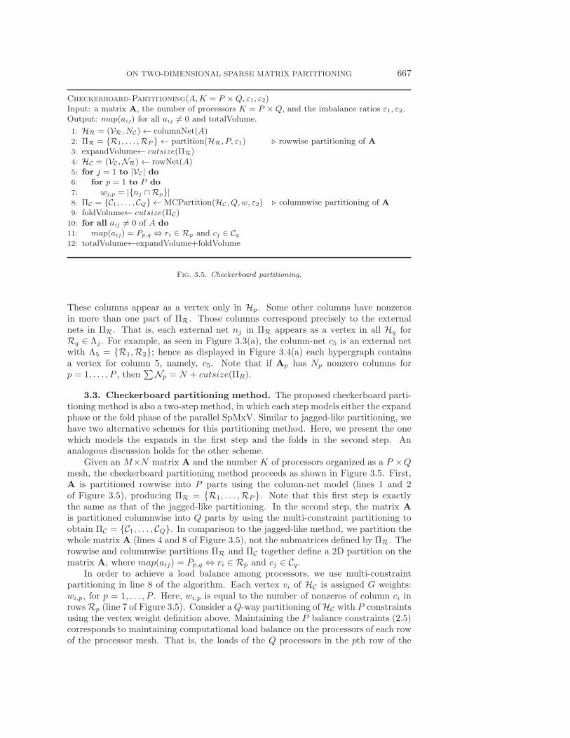
Checkerboard-Partitioning(A,K = P ×Q, ε1, ε2)Input: a matrix A, the number of processors K = P ×Q, and the imbalance ratios ε1, ε2.Output: map(aij) for all aij �= 0 and totalVolume.
1: HR = (VR, NC)← columnNet(A)2: ΠR = {R1, . . . ,RP } ← partition(HR, P, ε1) � rowwise partitioning of A3: expandVolume← cutsize(ΠR)4: HC = (VC ,NR)← rowNet(A)5: for j = 1 to |VC | do6: for p = 1 to P do7: wj,p = |{nj ∩Rp}|8: ΠC = {C1, . . . , CQ} ← MCPartition(HC , Q,w, ε2) � columnwise partitioning of A9: foldVolume← cutsize(ΠC)
10: for all aij �= 0 of A do11: map(aij) = Pp,q ⇔ ri ∈ Rp and cj ∈ Cq12: totalVolume←expandVolume+foldVolume
Fig. 3.5. Checkerboard partitioning.
These columns appear as a vertex only in Hp. Some other columns have nonzerosin more than one part of ΠR. Those columns correspond precisely to the externalnets in ΠR. That is, each external net nj in ΠR appears as a vertex in all Hq forRq ∈ Λj. For example, as seen in Figure 3.3(a), the column-net c5 is an external netwith Λ5 = {R1,R2}; hence as displayed in Figure 3.4(a) each hypergraph containsa vertex for column 5, namely, c5. Note that if Ap has Np nonzero columns forp = 1, . . . , P , then
∑Np = N + cutsize(ΠR).
3.3. Checkerboard partitioning method. The proposed checkerboard parti-tioning method is also a two-step method, in which each step models either the expandphase or the fold phase of the parallel SpMxV. Similar to jagged-like partitioning, wehave two alternative schemes for this partitioning method. Here, we present the onewhich models the expands in the first step and the folds in the second step. Ananalogous discussion holds for the other scheme.
Given an M×N matrix A and the number K of processors organized as a P ×Qmesh, the checkerboard partitioning method proceeds as shown in Figure 3.5. First,A is partitioned rowwise into P parts using the column-net model (lines 1 and 2of Figure 3.5), producing ΠR = {R1, . . . ,RP }. Note that this first step is exactlythe same as that of the jagged-like partitioning. In the second step, the matrix Ais partitioned columnwise into Q parts by using the multi-constraint partitioning toobtain ΠC = {C1, . . . , CQ}. In comparison to the jagged-like method, we partition thewhole matrix A (lines 4 and 8 of Figure 3.5), not the submatrices defined by ΠR. Therowwise and columnwise partitions ΠR and ΠC together define a 2D partition on thematrix A, where map(aij) = Pp,q ⇔ ri ∈ Rp and cj ∈ Cq.
In order to achieve a load balance among processors, we use multi-constraintpartitioning in line 8 of the algorithm. Each vertex vi of HC is assigned G weights:wi,p, for p = 1, . . . , P . Here, wi,p is equal to the number of nonzeros of column ci inrowsRp (line 7 of Figure 3.5). Consider aQ-way partitioning ofHC with P constraintsusing the vertex weight definition above. Maintaining the P balance constraints (2.5)corresponds to maintaining computational load balance on the processors of each rowof the processor mesh. That is, the loads of the Q processors in the pth row of the

668 UMIT V. CATALYUREK, CEVDET AYKANAT, AND BORA UCAR
C1 C2
r2
r3
r4
r5r6
r7
r8
r9
r10
r11 r12
r13
r14
r15
r16
c1
c2
c3
c4
c5
c6
c7
c8
c9c10
c11
c12
c13
c14
c15
c16
r1
W1(1) = 12W1(2) = 12
W2(1) = 12W2(2) = 11
(a)
3 6 11 14 1 5 10 13 4 8 12 16 2 7 9 15
3
6
11
14
1
5
10
13
4
8
12
16
2
7
9
15
nnz = 47vol = 8 imbal = [ 6.4%, 2.1%]
(b)
Fig. 3.6. Second step of 4-way checkerboard partitioning: (a) 2-way multi-constraint partition-ing ΠC of row-net hypergraph representation HC of A; (b) Final checkerboard partitioning of Ainduced by (ΠR,ΠC); the nonzeros in the same partition are shown with the same shape and color;the deviation of the minimum and maximum numbers of nonzeros of a part from the average aredisplayed as an interval imbal; nnz and vol denote, respectively, the number of nonzeros and thetotal communication volume.
processor mesh satisfiesWp,q ≤ (1+ε2)∑
i wi,p
Q . We also have∑
i wi,p ≤ (1+ε1)nnz (A)
P ,due to the P -way ε1-balanced partitioning in line 2. As in the jagged-like partitioning,the resulting K-way partitioning of A is guaranteed to satisfy a balance constraintwith an allowable imbalance ratio of ε = (ε1 + ε2 + ε1ε2).
Establishing the equivalence between the total communication volume and thesum of the cutsizes of the two partitions is fairly straightforward. We observe that ifthe nonzeros in the ith row of A are partitioned among q processors, then the row-net ri of HC will connect q parts after the columnwise partitioning in line 8 of thealgorithm. That is, the volume of communication for the fold operations correspondsexactly to the cutsize(ΠC). Similarly, if the nonzeros in the jth column of A arepartitioned among p processors, then the net cj of HR should have vertices in thesame set of parts after the rowwise partitioning in line 2 of the algorithm. That is,the volume of communication for the expand operations corresponds exactly to thecutsize(ΠR).
We demonstrate the main steps of the proposed checkerboard partitioning methodon the sample matrix shown in Figure 2.1 for a 2× 2 processor mesh. First, a 2-wayrowwise partition ΠR is obtained, giving the same figure as shown in Figure 3.3.Figure 3.6(a) displays the row-net hypergraph representation HC of matrix A. It alsoshows a 2-way multi-constraint partition ΠC of HC . In Figure 3.6(a), w9,1 = 0 andw9,2 = 4 for internal column c9 of row stripe R2, whereas w5,1 = 2 and w5,2 = 4 forexternal column c5. Figure 3.6(b) displays the 2×2 checkerboard partition inducedby (ΠR,ΠC).
Compared to the jagged-like partitioning method, the checkerboard partitioningmethod maintains both row and column coherences at the level of the row or columnsof the processor mesh. It confines the expand and fold communications to the pro-cessors of the same column and row of the processor mesh, respectively. In this way,the number of messages to be sent and received by a processor is limited to P − 1 andQ− 1 processors in the expand and fold phases, respectively.

ON TWO-DIMENSIONAL SPARSE MATRIX PARTITIONING 669
4. Further investigations and comments.
4.1. Comparison of the models. 1D rowwise partitioning incurs only expandcommunication, because it respects row coherence by assigning entire rows to proces-sors while disturbing column coherence. In a dual manner, 1D columnwise partitioningincurs only fold communication, because it respects column coherence by assigningentire columns to processors while disturbing row coherence. Therefore, in the 1Dmatrix partitioning, the number of messages sent by a processor may be as high asK − 1, for a parallel system with K processors, giving a total of K(K − 1) messages.In a rowwise partitioning, the worst-case total communication volume is (K − 1)Nfor an M×N matrix, and this worst case occurs when each column has at least onenonzero in each row stripe. Similarly, for a columnwise partitioning, the worst-casetotal communication volume is (K − 1)M .
In the fine-grain partitioning method, nonzeros are allowed to be assigned indi-vidually to processors. Since neither row coherence nor column coherence is enforced,this method may incur both expand and fold operations, and hence the number ofmessages sent by a processor may be as high as 2(K− 1), giving a total of 2K(K− 1)messages. The worst-case communication volume is (K − 1)(M + N) units in to-tal. The proposed fine-grain hypergraph partitioning model is highly flexible, sinceit enables assignment of each nonzero entry individually—it can partition a givenmatrix among Z processors as compared to, for example, M processors in rowwisepartitioning. The fine-grain model has a higher degree of freedom than the 1D mod-els in minimizing communication volume, since it enforces neither row coherence norcolumn coherence.
The jagged-like partitioning is intrinsically better than the fine-grain partitioningin terms of the total number of messages. In the expand communication phase, themaximum number of messages per processor is P × Q − Q = K − Q for a P × Qmesh of processors, since the processors in the same row of the processor mesh do notrequire communication of x-vector components. In the fold communication phase, themaximum number of messages per processor isQ−1, since row coherence is maintainedat the level of rows of the processor mesh. Hence, the upper bound on the total numberof messages in jagged-like partitioning is K(K − Q) +K(Q − 1) = K(K − 1). Thetotal communication volume may be as high as (P − 1)N +(Q− 1)M , and this worstcase occurs when each row and column of each submatrix of A(k), as shown in (2.1),has at least one nonzero.
The 2D checkerboard partitioning method can be considered as a trade-off be-tween 1D partitioning and 2D fine-grain partitioning methods. This method respectsboth row and column coherences in a coarse level. It respects row coherence by as-signing entire matrix rows to the processors in the same row of the processor mesh. Italso respects column coherence by assigning entire matrix columns to the processorsin the same column of the processor mesh. In other words, this method confines theexpand and fold operations, respectively, to the columns and the rows of the processormesh. In this way, it reduces the maximum number of messages sent by a proces-sor to P + Q − 2 for a P ×Q mesh of processors; if P = Q =
√K, this results in
2K(√K − 1) messages in total. The total communication volume may be as high as
(P − 1)N + (Q− 1)M , and this worst case occurs when each row and column of eachsubmatrix has at least one nonzero.
4.2. Modeling collective communication. As discussed above, the proposedjagged-like partitioning method confines the communication regarding y-vector entriesto a row of the processor mesh; i.e., each yi will be computed by at most Q processors.

670 UMIT V. CATALYUREK, CEVDET AYKANAT, AND BORA UCAR
The checkerboard partitioning approach goes one step further and also confines thecommunications regarding the x-vector entries to a column of the processor mesh;i.e., each xj is needed by at most P processors. Since P and Q are usually muchsmaller than K, all-to-all communication looks affordable in the row-column-parallelmultiply algorithm given in section 2.1. More precisely, if jagged-like or checkerboardpartitioning approaches are used, steps 4 and 5 of the row-column-parallel SpMxValgorithm given in section 2.1 can be replaced by an optimized all-to-all reductionoperation. If the checkerboard partitioning approach is used, then steps 1 and 2 ofthe same algorithm can be replaced by an optimized all-to-all broadcast operation.Those collective communication operations can be implemented for any number ofprocessors [24]; i.e., the number of processors is not restricted to the powers of two.The attractive feature of this all-to-all communication scheme is that it reduces themaximum number of messages per processor to �logP or �logQ in the expand or foldcommunication phases. When such an optimized all-to-all scheme is used, the totalcommunication volume can be minimized by reducing the total number of x-vectorentries expanded or y-vector entries folded. Clearly, the objective here is equivalentto reducing the number columns and rows whose nonzeros are shared by more thanone processor. The models proposed in this work can be directly used to address thisproblem by using the cut-net objective function (2.3) instead of the connectivity-1objective function (2.4).
4.3. How to apply hypergraph-based partitioning to other applications.Although we have exclusively considered the SpMxV, there are other applications thatcan make use of the contributions of the current work—in general, matrix partition-ing methods. Parallel reduction (aggregation) operations form a significant class ofsuch applications [16, 18]. The reduction operation consists of computing M outputelements using N input elements. An output element may depend on multiple inputelements, and an input element may contribute to multiple output elements. Assumethat the operation on which reduction is performed is commutative and associative.Then, the inherent computational structure can be represented with an M×N depen-dency matrix, where each row and column of the matrix represents an output elementand an input element, respectively. For an input element xj and an output elementyi, if yi depends on xj , aij is set to 1 (otherwise zero). Using this representation, theproblem of partitioning the workload for the reduction operation is equivalent to theproblem of partitioning the dependency matrix for efficient SpMxV [13, 29].
In some other reduction problems, the input and output elements may be pre-assigned to parts. The proposed hypergraph model can be accommodated to thoseproblems by adding K part vertices and connecting those vertices to the nets whichcorrespond to the pre-assigned input and output elements. Obviously, those partvertices must be fixed to the corresponding parts during the partitioning. Since therequired property is already included in the existing hypergraph partitioners [1, 6, 10,28], this does not add extra complexity to our methods.
4.4. A recipe for matrix partitioning. The following abbreviations will beused here and hereafter for the matrix partitioning methods discussed so far:
• RW: Rowwise 1D partitioning,• CW: Columnwise 1D partitioning,• FG: Fine-grain 2D partitioning,• JL: Jagged-like 2D partitioning,• CH: Checkerboard 2D partitioning.

ON TWO-DIMENSIONAL SPARSE MATRIX PARTITIONING 671
As discussed so far, the FG method is most likely to give better total communica-tion volume and computational load balance than any other method discussed. How-ever, it is also most likely to be the slowest. The CHmethod, on the other hand, shouldbe the fastest, it most likely obtains better total number of messages than any of theothers, but it is likely to obtain the worst total communication volume and the worstcomputational load balance. The JL method should be in between these two methodsin almost any metric considered. Except in extremely skewed matrices, 1D partition-ing methods can never be significantly better than all of the remaining methods.
As there are a number of alternative partitioning methods, each with a differenttrait, a means to automate the decision of choosing which alternative to partition agiven matrix is necessary. If any of the metrics mentioned above is significantly moreimportant than the others, then the best method should be chosen. For example, ifthe total number of messages is of utmost importance, then the checkerboard parti-tioning method seems to be the method of choice, as it has the lowest limit for thismetric. However, usually a combination of the communication metrics, including themaximum volume and message sent by a processor [47] or these two quantities bothin terms of sends and receives [3], corresponds to the communication cost. Usually,a user of the partitioning methods does not have to know all the details of the parti-tioning methods. Therefore, we present a recipe that tries to suggest a partitioningmethod for a given matrix, where the suggestions are made for the total communi-cation volume, meanwhile trying to reduce the other metrics on the average. Noticethat for metrics other than the total volume of communication, different recipes canbe developed. As the principal aim of hypergraph partitioning models is to minimizethe total communication volume, we think that a recipe based on this metric couldbe the most accurate and beneficial one. Note that for 1D partitioning methods, ithas been already said that it is advisable to partition along the columns (rows) ifthe given matrix has dense rows (columns) but no dense columns (rows) [21]. Thisadvice, although it is sound for 1D partitioning, is not adequate for 2D partitioning,as neither row coherence nor column coherence is guaranteed to be respected.
The proposed recipe is shown in Figure 4.1. A user provides a matrix A, numberof processors K and an imbalance ratio ε (usually less than 3%) to use the recipe.A number of quantities are then computed and compared with certain thresholdvalues to suggest a method. The recipe uses the pattern symmetry score, Sym(A) =∑
pijpijpji/Z, where pij = 1 if aij �= 0 and zero otherwise and a number of statistical
descriptions of the row degrees (shown with dr) and the column degrees (shown withdc). In the recipe, max, avg, and med represent, respectively, the maximum, average,and median; mode is the value that has the largest number of occurrences; e.g.,mode(dr) is the most occurring row degree. Q3 is the third quartile; e.g., Q3(dc)is a number which is greater than 75% of the column degrees and smaller than therest. Note that all these numbers, including the symmetry score, can be computed inO(Z +M +N) time—see [14, Chapter 10] for median and order statistics and [45, p.720] for calculating the symmetry score.
The recipe has three sets of tests to suggest a method: one set for rectangularmatrices, one set for square and almost symmetric (with a pattern symmetry scorelarger than 0.95) matrices, and another set for the remaining square unsymmetricmatrices. For a rectangular matrix, if it is a very tall or very wide matrix, it selectsthe CW or the RW method, respectively; otherwise it chooses the FG method. Forsquare matrices, it chooses the FG method for pathological cases—when the numberof nonzeros is less than the number of rows (Z ≤M) and mode of the row or columndegrees is zero; the same choice is made for those matrices where the CH or JL

672 UMIT V. CATALYUREK, CEVDET AYKANAT, AND BORA UCAR
sym(A) > 0.95
Partitioning Recipe
Square?
Yes
FGS/FGU JLS/JLU
Yes No
Yes
CWU
Yes
RWU
Yes
FGU
NoNo
Pathological? or or
or
No
FGS/FGU
Yes
FGU
Yes
JLUT
Yes
JLU
No
No
Noor
No
M < 0.35N
N < 0.35M
(M = N?)
M ≥ Z mode(dr, dc) = 0M/
√K < max(dr, dc)
max(dr, dc) ≥ (1 − ε)2Z/√
K
avg(dr) > med(dr)
Q3(dr)-med(dr) < max(dr)−Q3(dr)2
Q3(dc)-med(dc) < max(dc)−Q3(dc)2
med(dr) ≤med(dc)
Fig. 4.1. A recipe for matrix partitioning. Matrix A is of size M ×N with Z nonzeros to bepartitioned among K processors. The arrays dr and dc represent the row and column degrees; i.e.,dr(i) is the number of nonzeros in row i.The statistical descriptors max, avg, and med represent,respectively, the maximum, average, and median; mode is the value that has the largest number ofoccurrences. Q3 is the third quartile; e.g., Q3(dc) is a number which is greater than 75% of thecolumn degrees. Sym(A) measures the symmetry score, and ε is a user specified allowed imbalanceratio. Letters S and U after the method names (RW, CW, FG, JL, CH) represent symmetric andunsymmetric vector partitioning, respectively.
methods could lead to a load imbalance or have a hard time obtaining balance, i.e.,max(dr, dc) ≥ (1 − ε)2Z/
√K. For pattern symmetric or almost pattern symmetric
matrices (i.e., Sym(A) > 0.95), the recipe chooses the FG method, if the averagerow/column degree is greater than the median; otherwise it chooses the JL method.Note that in any case a symmetric vector partitioning is always suggested for thesetypes of matrices. For the unsymmetric square matrices with Sym(A) ≤ 0.95, therecipe chooses the FG method, if there is a certain relation among the median, thirdquartile, and the maximum of the row or column degrees; otherwise a variant of JLpartitioning is suggested. For these matrices, the recipe uses the JL method thatperforms columnwise partitioning first (JLT ) when the median of the row degrees issmaller than that of the column degrees. The tests avg(dr) > med(dr) and the big onewith the quartiles try to see if there are sufficiently large numbers of rows or columnswith a high number of nonzeros. With the aid of the test med(dr) ≤ med(dc), therecipe tries to adapt the advice on 1D partitioning to the JL method; i.e., if themedian degree of the rows is smaller than the median degree of the columns, thenmost probably there are more dense rows than columns, and hence partitioning alongthe columns in the first step is advisable. With this test, the recipe also tries to leavemore flexibility to the second phase of the JL partitioning method in terms of loadbalancing.

ON TWO-DIMENSIONAL SPARSE MATRIX PARTITIONING 673
5. Experimental results. We performed an extensive experimental evaluationof the proposed 2D sparse matrix partitioning methods as well as 1D partitioningmethods [9] using almost all large matrices of the University of Florida (UFL) sparsematrix collection [15]. Here, we first present the results of this experimental evaluationand then investigate the effectiveness of the partitioning recipe.
5.1. Test dataset and experimental setup. We ran our tests using the newlydeveloped PaToH Matlab Matrix-Partitioning Interface [10, 51] (PaToH and Mat-lab Matrix-Partitioning Interface are available at http://bmi.osu.edu/˜umit/software.html) on a 32-node cluster owned by the Department of Biomedical Informatics at TheOhio State University. Each computer is equipped with dual 2.4 GHz Opteron 250processors, 8 GB of RAM, and 500 GB of local storage. Nodes are interconnected bya switched Infiniband network. We ran PaToH using default parameters. In orderto facilitate the running of thousands of sequential partitionings via Matlab inter-face, we developed a simple first-in-first-out job scheduler and Matlab script executer,dcexec, using DataCutter [2], that runs each partitioning one-by-one on one of theavailable nodes. The script dcexec keeps an instance of Matlab running on each nodeand passes Matlab partitioning commands via the use of a FIFO file, hence avoidingMatlab startup overhead for each partitioning.
We excluded matrices that have less than 500 nonzeros. Since our testing envi-ronment is based on sequential partitioning of the matrices within the Matlab envi-ronment, we also excluded matrices that have more than 10,000,000 nonzeros. Therewere 1,413 matrices in the UFL collection satisfying these properties (there were atotal of 1,877 matrices at the time of experimentation among which 57 had more than10,000,000 nonzeros). We tested with K ∈ {4, 16, 64, 256}. For a specific K value, K-way partitioning of a test matrix constitutes a partitioning instance. The partitioninginstances in which min{M,N} < 50 × K are discarded, as the parts would becometoo small to be meaningful. These resulted in 4,100 partitioning instances, amongwhich 1,932 were with a symmetric matrix, 1,456 were with a square unsymmetricmatrix, and 712 were with a rectangular matrix (on 45 instances M > N and on 667instances M < N).
5.2. Partitioning methods. We tested all five partitioning methods RW, CW,FG, JL and CH for every partitioning instance. We also include the results ofthe recipe discussed in section 4.4. As discussed before, the recipe, being a meta-partitioning method, chooses a partitioning method from the above list, using somematrix statistics, and applies the chosen partitioning method.
We considered symmetric and nonsymmetric vector partitioning for square ma-trices. In the symmetric case, we added missing diagonal entries to the matricesbefore partitioning and assigned the vector entries to the parts which contained thecorresponding diagonal entry. In the nonsymmetric vector partitioning case, we useda simple approach to assign vector entries after the matrix partitioning. In this ap-proach, each vector entry xj or yi was assigned to a part having at least one nonzeroin the corresponding column (the jth column) or row (the ith row), respectively, ofA. If more than one part was qualified for assignment, we arbitrarily picked the onewith the least number of vector entries assigned so far.
For checkerboard and jagged-like partitioning, our default approach partitions thematrix rowwise in the first step and columnwise in the second step. For complete-ness, for unsymmetric matrices we also considered changing the order of partitioningdirection, which is achieved by taking the transpose of the input matrix prior to parti-

674 UMIT V. CATALYUREK, CEVDET AYKANAT, AND BORA UCAR
tioning. Reported results for checkerboard and jagged-like partitioning include theseadditional methods, and they are referred to as JLT and CHT .
As PaToH involves randomized algorithms, we obtained 10 different partitionsfor each partitioning instance with every applicable method and used the average ofthe 10 partitionings as the representative result for that particular method on thatparticular partitioning instance. In all partitioning instances, maximum allowableimbalance ratio ε, see (2.2) and (2.5), is set to 3%. Although the balance constraint ismet in most of the partitionings, it was not feasible in some of the problem instances.We will try to point out the balance problems while explaining the results.
The jagged-like and checkerboard methods assume a virtual 2D processor mesh(see sections 3.2 and 3.3). In our experiments, for mesh dimensions P and Q weselected P = Q =
√K, for K ∈ {4, 16, 64, 256}. The multi-constraint partitioning
techniques have been observed to perform worse when the number of constraints isincreased [1, 49]. Therefore, for partitioning cases with P �= Q, we suggest partitioningfirst for the smaller of P and Q to have a smaller number of constraints in the secondphase of the checkerboard method.
5.3. Performance profiles. We use a generic tool, performance profiles, intro-duced by Dolan and More [17] for comparing a set of methods over a large set of testcases (in our case, the partitioning instances) with regard to a specific performancemetric. The main idea behind performance profiles is to use a cumulative distributionfunction for a performance metric, instead of, for example, taking averages over allthe test cases. We will compare the partitioning methods using the following metrics:the total communication volume, the total number of messages, the maximum vol-ume of messages sent by a single processor, the computational load imbalance, andthe partitioning time.
Each performance profile plot helps compare different methods with respect to aspecific metric. For a given metric, a profile plot shows the probability that a specificpartitioning method gives results which are within some value τ of the best resultreached by all methods. Therefore the higher the probability, the more preferablethe method is. For example, for the total communication volume metric, a τ valueshows the probability for a partitioning method that the total communication volumeobtained by that method is within τ of the best result reached by all methods shownin the same plot.
On 63 partitioning instances, the minimum total volume of communication foundby at least one partitioning method was zero. We exclude those instances while plot-ting the performance profiles. In the performance profiles for the rectangular matrices,the plots of RW, CW, FG, JL, and CH always refer to the results of the associatedpartitioning method, post-processed with a nonsymmetric vector partitioning. In theprofiles for the symmetric matrices, these labels always refer to the results of theassociated partitioning method with a symmetric vector partitioning (and hence themissing diagonal entries are always added to the matrices before partitioning). Theunsymmetric square case is a little more complicated. For these matrices, RW, CW,and FG always refer to the best result (with respect to the total communicationvolume) of the associated method with a symmetric and nonsymmetric vector par-titioning (in the symmetric vector partitioning case the missing diagonal entries areadded). JL and CH, in addition to the two different vector partitioning approaches,also include the best of the transposed partitioning approaches, i.e., JLT and CHT . Inthe performance profile figures labeled with “all instances,” each method refers to the

ON TWO-DIMENSIONAL SPARSE MATRIX PARTITIONING 675
best of symmetric (whenever applicable), nonsymmetric, and transposed approaches(whenever applicable). We did not use transposed approaches on the rectangularmatrices, as this will change the size of the matrices. The symmetric matrices usu-ally require symmetric vector partitioning (for example, in linear system solvers forsymmetric matrices). In unsymmetric matrices, all methods with all variations areacceptable. With the “all instances” figures, we mean to show what can be expectedwhen a certain partitioning approach is used with all variations; e.g., a user of thesepartitioning methods tries all possible combinations at hand and uses the best (interms of the total communication volume).
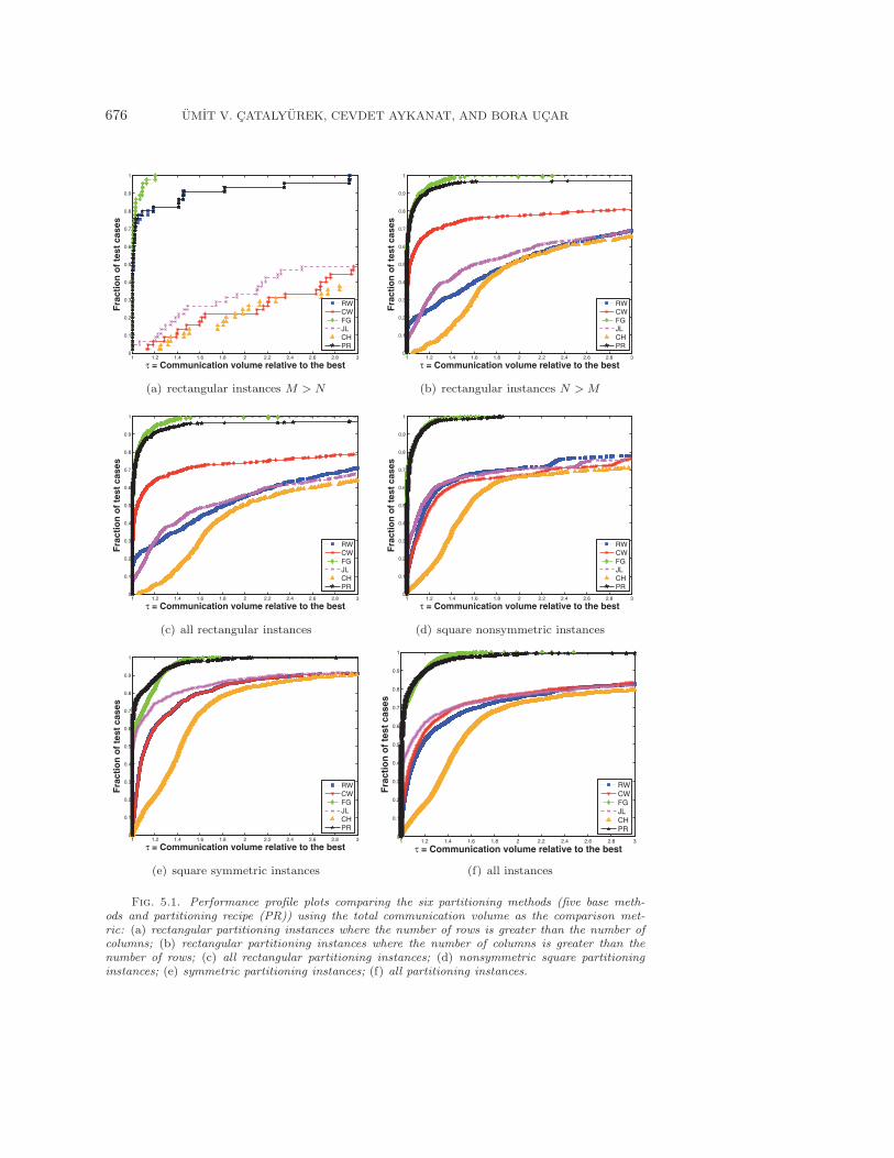
5.4. Results. Figure 5.1 displays performance profiles of five partitioning meth-ods as well as the proposed recipe, using the total communication volume as the com-parison metric. As seen in Figure 5.1(f), in almost 90% of the partitioning instancesthe FG method obtains results within 1.2 of the best. In rectangular instances (Fig-ures 5.1(a)–5.1(c)), when the number of rows is greater than the number of columns(i.e., M > N , Figure 5.1(a)), as one might expect, the RW method produces thesecond-best results, and when the number of columns is greater than the number ofrows (Figure 5.1(b)), the CW method produces the second-best results. When weconsider all rectangular instances (Figure 5.1(c)), since there are a lot more instanceswith more columns than rows (662 vs 45—here 5 matrices were discarded because theyhad zero total communication volume), the CW method still produces the second-bestresults. In all different types of instances, CH produces the worst results because itis the most restricted partitioning method. However, in almost 75% of partitioninginstances even CH results are within 2 of the best.
Figure 5.2 displays the comparison of the methods using the total number ofmessages as the comparison metric. As seen in the figure, this is the metric for whichCH shines, as it inherently limits the maximum number of messages to a much smallernumber than the others. In almost 75% of the partitioning instances, it produces theleast number of messages, and in 95% of the partitioning instances, it produces theresults within 1.5 of the best. Although the upper bound on the total number ofmessages for the JL method is the same as those for the RW and CW methods(K(K − 1)), JL seems to be preferable for square matrices (for rectangular matrices,if M > N , RW is preferable, else CW is preferable). As expected, FG achieves theworst performance in this metric.
Figure 5.3 displays the comparisons on the metrics of the maximum volume andmaximum number of messages of a processor. Since the trends in these two metricsare similar to those of the total volume and the total number of messages, we presenta single performance profile plot for each of those metrics (containing all instances).In terms of the maximum volume per processor metric, FG and JL generally producebetter results. The CH method produces more pronounced best results for the maxi-mum number of messages per processor metric, since its upper bound is the smallestamong all. In almost 85% of the partitioning instances, CH produces the best results.
Figure 5.4(a) displays the comparison of average imbalance ratios of the compu-tational loads of the processors. In 1,411 partitioning instances (about 35% of thewhole), one of the methods found a perfect balance; that is, the best ε was 0, see (2.2)and (2.5). Hence, the plots do not reach up to 1 in the y-axis of the performanceprofile plots. As expected, FG achieves better partitionings in terms of imbalanceratios because it does its assignments in the finest granularity possible. Actually, FGfound partitions with perfect balance in 1,266 partitioning instances. Recall that theCH and JL methods are two-step methods, and unfortunately solution of the first step
676 UMIT V. CATALYUREK, CEVDET AYKANAT, AND BORA UCAR
1 1.2 1.4 1.6 1.8 2 2.2 2.4 2.6 2.8 30
0.1
0.2
0.3
0.4
0.5
0.6
0.7
0.8
0.9
1
τ = Communication volume relative to the best
Fra
ctio
n o
f te
st c
ases
RWCWFGJLCHPR
(a) rectangular instances M > N
1 1.2 1.4 1.6 1.8 2 2.2 2.4 2.6 2.8 30
0.1
0.2
0.3
0.4
0.5
0.6
0.7
0.8
0.9
1
τ = Communication volume relative to the best
Fra
ctio
n o
f te
st c
ases
RWCWFGJLCHPR
(b) rectangular instances N > M
1 1.2 1.4 1.6 1.8 2 2.2 2.4 2.6 2.8 30
0.1
0.2
0.3
0.4
0.5
0.6
0.7
0.8
0.9
1
τ = Communication volume relative to the best
Fra
ctio
n o
f te
st c
ases
RWCWFGJLCHPR
(c) all rectangular instances
1 1.2 1.4 1.6 1.8 2 2.2 2.4 2.6 2.8 30
0.1
0.2
0.3
0.4
0.5
0.6
0.7
0.8
0.9
1
τ = Communication volume relative to the best
Fra
ctio
n o
f te
st c
ases
RWCWFGJLCHPR
(d) square nonsymmetric instances
1 1.2 1.4 1.6 1.8 2 2.2 2.4 2.6 2.8 30
0.1
0.2
0.3
0.4
0.5
0.6
0.7
0.8
0.9
1
τ = Communication volume relative to the best
Fra
ctio
n o
f te
st c
ases
RWCWFGJLCHPR
(e) square symmetric instances
1 1.2 1.4 1.6 1.8 2 2.2 2.4 2.6 2.8 30
0.1
0.2
0.3
0.4
0.5
0.6
0.7
0.8
0.9
1
τ = Communication volume relative to the best
Fra
ctio
n o
f te
st c
ases
RWCWFGJLCHPR
(f) all instances
Fig. 5.1. Performance profile plots comparing the six partitioning methods (five base meth-ods and partitioning recipe (PR)) using the total communication volume as the comparison met-ric: (a) rectangular partitioning instances where the number of rows is greater than the number ofcolumns; (b) rectangular partitioning instances where the number of columns is greater than thenumber of rows; (c) all rectangular partitioning instances; (d) nonsymmetric square partitioninginstances; (e) symmetric partitioning instances; (f) all partitioning instances.

ON TWO-DIMENSIONAL SPARSE MATRIX PARTITIONING 677
1 1.5 2 2.5 3 3.5 4 4.5 50
0.1
0.2
0.3
0.4
0.5
0.6
0.7
0.8
0.9
1
τ = Number of messages relative to the best
Fra
ctio
n o
f te
st c
ases
RWCWFGJLCHPR
(a) rectangular instances M > N
1 1.5 2 2.5 3 3.5 4 4.5 50
0.1
0.2
0.3
0.4
0.5
0.6
0.7
0.8
0.9
1
τ = Number of messages relative to the best
Fra
ctio
n o
f te
st c
ases
RWCWFGJLCHPR
(b) rectangular instances N > M
1 1.5 2 2.5 3 3.5 4 4.5 50
0.1
0.2
0.3
0.4
0.5
0.6
0.7
0.8
0.9
1
τ = Number of messages relative to the best
Fra
ctio
n o
f te
st c
ases
RWCWFGJLCHPR
(c) all rectangular instances
1 1.5 2 2.5 3 3.5 4 4.5 50
0.1
0.2
0.3
0.4
0.5
0.6
0.7
0.8
0.9
1
τ = Number of messages relative to the best
Fra
ctio
n o
f te
st c
ases
RWCWFGJLCHPR
(d) square nonsymmetric instances
1 1.5 2 2.5 3 3.5 4 4.5 50
0.1
0.2
0.3
0.4
0.5
0.6
0.7
0.8
0.9
1
τ = Number of messages relative to the best
Fra
ctio
n o
f te
st c
ases
RWCWFGJLCHPR
(e) square symmetric instances
1 1.5 2 2.5 3 3.5 4 4.5 50
0.1
0.2
0.3
0.4
0.5
0.6
0.7
0.8
0.9
1
τ = Number of messages relative to the best
Fra
ctio
n o
f te
st c
ases
RWCWFGJLCHPR
(f) all instances
Fig. 5.2. Performance profile plots comparing the six partitioning methods using the total num-ber of messages as the comparison metric: (a) rectangular partitioning instances where the number ofrows is greater than the number of columns; (b) rectangular partitioning instances where the numberof columns is greater than the number of rows; (c) all rectangular partitioning instances; (d) non-symmetric square partitioning instances; (e) symmetric partitioning instances; (f) all partitioninginstances.
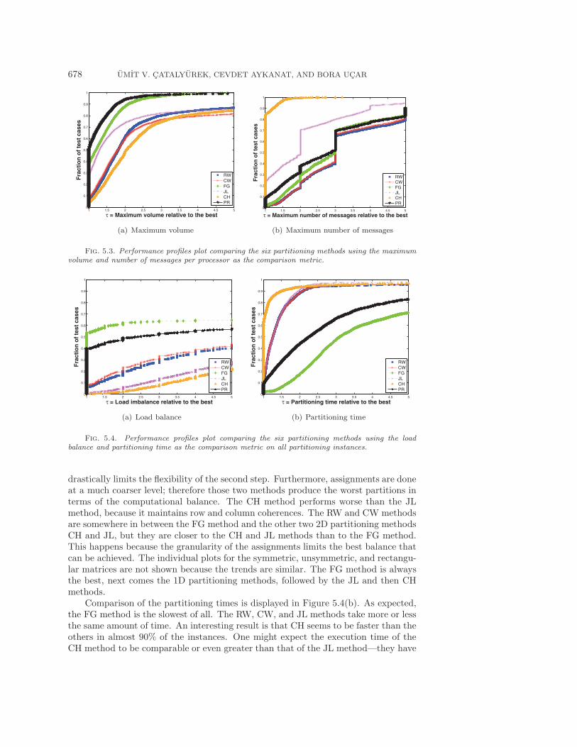
678 UMIT V. CATALYUREK, CEVDET AYKANAT, AND BORA UCAR
1 1.5 2 2.5 3 3.5 4 4.5 50
0.1
0.2
0.3
0.4
0.5
0.6
0.7
0.8
0.9
1
τ = Maximum volume relative to the best
Fra
ctio
n o
f te
st c
ases
RWCWFGJLCHPR
(a) Maximum volume
1 1.5 2 2.5 3 3.5 4 4.5 50
0.1
0.2
0.3
0.4
0.5
0.6
0.7
0.8
0.9
1
τ = Maximum number of messages relative to the best
Fra
ctio
n o
f te
st c
ases
RWCWFGJLCHPR
(b) Maximum number of messages
Fig. 5.3. Performance profiles plot comparing the six partitioning methods using the maximumvolume and number of messages per processor as the comparison metric.
1 1.5 2 2.5 3 3.5 4 4.5 50
0.1
0.2
0.3
0.4
0.5
0.6
0.7
0.8
0.9
1
τ = Load imbalance relative to the best
Fra
ctio
n o
f te
st c
ases
RWCWFGJLCHPR
(a) Load balance
1 1.5 2 2.5 3 3.5 4 4.5 50
0.1
0.2
0.3
0.4
0.5
0.6
0.7
0.8
0.9
1
τ = Partitioning time relative to the best
Fra
ctio
n o
f te
st c
ases
RWCWFGJLCHPR
(b) Partitioning time
Fig. 5.4. Performance profiles plot comparing the six partitioning methods using the loadbalance and partitioning time as the comparison metric on all partitioning instances.
drastically limits the flexibility of the second step. Furthermore, assignments are doneat a much coarser level; therefore those two methods produce the worst partitions interms of the computational balance. The CH method performs worse than the JLmethod, because it maintains row and column coherences. The RW and CW methodsare somewhere in between the FG method and the other two 2D partitioning methodsCH and JL, but they are closer to the CH and JL methods than to the FG method.This happens because the granularity of the assignments limits the best balance thatcan be achieved. The individual plots for the symmetric, unsymmetric, and rectangu-lar matrices are not shown because the trends are similar. The FG method is alwaysthe best, next comes the 1D partitioning methods, followed by the JL and then CHmethods.
Comparison of the partitioning times is displayed in Figure 5.4(b). As expected,the FG method is the slowest of all. The RW, CW, and JL methods take more or lessthe same amount of time. An interesting result is that CH seems to be faster than theothers in almost 90% of the instances. One might expect the execution time of theCH method to be comparable or even greater than that of the JL method—they have

ON TWO-DIMENSIONAL SPARSE MATRIX PARTITIONING 679
Table 5.1
The number of times a method produced the best result in terms of the total communicationvolume. If two or more methods give the same best value, each one’s score is incremented by one.
Method K = 4 K = 16 K = 64 K = 256RW sym 76 7 2 1CW sym 62 8 3 2FG sym 276 278 168 113JL sym 158 159 111 69CH sym 21 0 0 0RW nonsym 139 52 26 9CW nonsym 167 113 44 15FG nonsym 508 481 310 179JL nonsym 231 190 121 76CH nonsym 38 0 0 0JLT nonsym 78 53 39 29JLT sym 31 13 26 10CHT nonsym 19 0 0 0CHT sym 5 0 0 0PR 524 491 312 197
Table 5.2
The number of times a specific method was chosen by the partitioning recipe for 4,100 parti-tioning instances.
Method K = 4 K = 16 K = 64 K = 256FG sym 350 331 252 148JL sym 296 272 176 107RW nonsym 9 8 5 4CW nonsym 94 82 52 26FG nonsym 594 567 327 198JL nonsym 31 23 16 12JLT nonsym 43 40 24 13
the same first step, but the second step of CH involves multi-constraint partitioning.The CH method partitions a larger hypergraph in the second step, whereas the JLmethod partitions
√K smaller hypergraphs. We think that the more restricted search
space of the multi-constraint partitioning may result in such an outcome. Note thatthe individual plots for the symmetric, unsymmetric, and rectangular matrices arenot shown, as the trends are again similar to those that are shown. Up until τ = 2,the CH method is the fastest, followed by the almost equally fast RW, CW, and JLmethods, with the slowest always being the FG method. After τ = 2, all methodsexcept FG are nearly equally fast, and FG is again the slowest.
5.5. Evaluation of the recipe. In this section, we try to see how successfulthe recipe is in reducing the total communication volume and addressing the othercommunication cost metrics. Tables 5.1 and 5.2 display the number of times a methodproduced the best result in terms of total communication volume, and the numberof times a specific method was chosen by the partitioning recipe, respectively. Asseen in Table 5.1, FG produces the best results in terms of the total communicationvolume metric in a considerably larger number of instances than any other method.Note that in this table, the best is defined in absolute terms; e.g., even if a methodperforms slightly better than the others, its score is incremented by one. If any twomethods obtain the same best value, then each one’s score is incremented by one. Inother words, this table can be used to draw the performance profile of the methodsat τ = 1. We use Table 5.1 in order to highlight the choices made by the partitioning

680 UMIT V. CATALYUREK, CEVDET AYKANAT, AND BORA UCAR
recipe. Although selecting the FG method will most likely guarantee a better success(in terms of the total volume of communications metric) than any of the others, therecipe does not always choose the FG method; see Table 5.2. For example, for K = 4,it chooses FG in more than 900 instances, but it also chooses JL in more than 350instances, and 1D partitionings (RW or CW) in more than 100 instances. We note thatthe recipe obtains the highest number of best results for any K shown in the tables.
As shown in Figure 5.1(f), the recipe achieves a performance similar to that ofthe FG method (in almost 90% of the instances, the results obtained by these twomethods are within 1.2 of the best). Later we see that in almost 95% of the instancesboth results are within 1.4 of the best. Looking at Figures 5.2(d) and 5.2(e), we cansee that the recipe achieves better total number of messages than the FG method. InFigure 5.2(f), the difference between the recipe and the FG method is not significant.This is because of two reasons: first, on rectangular matrices, the FG method obtainsbetter results than the recipe; second, the recipe always chooses symmetric vectorpartitioning for the symmetric matrices, whereas FG is represented by the best of thesymmetric and nonsymmetric vector partitioning variants. As seen in Figure 5.3(a),the recipe and the FG methods obtain the best performance in the maximum volumeof a processor metric, with the recipe being more preferable up until τ = 2.5. As seenin Figure 5.3(b), in terms of the metric of the maximum number of messages of aprocessor, the recipe demonstrates an average behavior, being inferior to the CH andJL methods while being superior to the others. Now consider, in return, Figures 5.4(a)and 5.4(b). As seen from these figures, the recipe is faster than the FG method, whilethe difference between the computational load balance performances are acceptable.In summary, the proposed recipe achieves performance similar to the FG method interms of the total communication volume, while being more favorable or not too badin terms of the other metrics, on average. Therefore, for a user of these methods,we suggest using the proposed recipe to choose a partitioning method for obtaining agood partitioning on average.
6. Conclusion. We presented three hypergraph-based, 2D matrix partitioningmethods, each having a unique advantage. The fine-grain partitioning method treatsindividual nonzeros as the smallest assignable elements and hence achieves a veryfine-grain partitioning of matrices. This gives maximum flexibility in reducing thetotal communication volume and in balancing the computational loads at the ex-pense of longer partitioning time and possibly higher total number of messages. Thecheckerboard partitioning method produces coarser partitionings and maintains rowand column coherences at a coarse level by assigning rows and columns of the ma-trices to only a subset of processors. Hence, it imposes a smaller upper limit onthe total number of messages and the maximum number of messages of a processor.Although more restricted partitioning may yield larger total communication volume,this method could be a good alternative for parallel architectures with high messagelatency. The jagged-like method trades the number of messages limit for a bettercommunication volume.
We also presented a thorough experimental evaluation of the hypergraph-par-titioning-based methods using 4,100 partitioning instances—a partitioning instanceis defined as a pair of a matrix and an integer representing the number of parts.The experimentation clearly demonstrated the strengths and weaknesses of the pro-posed methods. The fine-grain model has the best performance in reducing the totalcommunication volume and the maximum volume of communication (measured interms of sends) of a processor; the checkerboard partitioning method has the best

ON TWO-DIMENSIONAL SPARSE MATRIX PARTITIONING 681
performance in reducing the total number of messages and the maximum number ofmessages (measured in terms of sends) of a processor; the jagged-like method alwaysstrikes a balance between the communication cost metrics best reduced by the fine-grain and checkerboard methods. We further proposed an easy-to-use partitioningrecipe that chooses one of the appropriate methods according to some matrix charac-teristics. The average behavior of the proposed recipe on the partitioning instances issuch that, with 90% probability, it produces results within 1.2 of the best solution forthe total volume of communication metric. Furthermore, the recipe achieves this per-formance while being faster than the partitioning method with the best performanceon the total communication volume metric on average, and while respecting a sym-metric vector partitioning for symmetric matrices. Although we are happy with theperformance of the recipe, we expect more accurate ones to be developed; those thatprioritize different communication cost metrics (the maximum number of messages ofa processor, for example) according to different target parallel machine architecturesand matrix sizes would be most useful.
REFERENCES
[1] C. Aykanat, B. B. Cambazoglu, and B. Ucar, Multi-level direct k-way hypergraph partition-ing with multiple constraints and fixed vertices, J. Parallel Distrib. Comput., 68 (2008),pp. 609–625.
[2] M. D. Beynon, T. Kurc, U. Catalyurek, C. Chang, A. Sussman, and J. Saltz, Distributedprocessing of very large datasets with DataCutter, Parallel Comput., 27 (2001), pp. 1457–1478.
[3] R. H. Bisseling and W. Meesen, Communication balancing in parallel sparse matrix-vectormultiplication, Electron. Trans. Numer. Anal., 21 (2005), pp. 47–65.
[4] T. Bultan and C. Aykanat, A new mapping heuristic based on mean field annealing, J.Parallel Distrib. Comput., 16 (1992), pp. 292–305.
[5] W. Camp, S. J. Plimpton, B. Hendrickson, and R. W. Leland, Massively parallel methodsfor engineering and science problems, Commun. ACM, 37 (1994), pp. 31–41.
[6] U. V. Catalyurek, E. G. Boman, K. D. Devine, D. Bozdag, R. Heaphy, and L. A. Fisk,Hypergraph-based dynamic load balancing for adaptive scientific computations, in Proceed-ings of the 21st International Parallel and Distributed Processing Symposium (IPDPS),2007, IEEE.
[7] U. V. Catalyurek, Hypergraph Models for Sparse Matrix Partitioning and Reordering, Ph.D.thesis, Bilkent University, Computer Engineering and Information Science, Ankara, Turkey,1999, http://www.cs.bilkent.edu.tr/tech-reports/1999/ABSTRACTS.1999.html.
[8] U. V. Catalyurek and C. Aykanat, Decomposing irregularly sparse matrices for parallelmatrix-vector multiplications, in Proceedings of the 3rd International Symposium on Solv-ing Irregularly Structured Problems in Parallel, Irregular’96, Lecture Notes in Comput.Sci. 1117, Springer-Verlag, New York, 1996, pp. 75–86.
[9] U. V. Catalyurek and C. Aykanat, Hypergraph-partitioning based decomposition for parallelsparse-matrix vector multiplication, IEEE Trans. Parallel Distrib. Syst., 10 (1999), pp. 673–693.
[10] U. V. Catalyurek and C. Aykanat, PaToH: A Multilevel Hypergraph Partitioning Tool,Version 3.0, Bilkent University, Department of Computer Engineering, Ankara, Turkey,1999. PaToH is available at http://bmi.osu.edu/˜umit/software.htm.
[11] U. V. Catalyurek and C. Aykanat, A fine-grain hypergraph model for 2D decomposition ofsparse matrices, in Proceedings of the 15th International Parallel and Distributed Process-ing Symposium (IPDPS), San Francisco, CA, 2001.
[12] U. V. Catalyurek and C. Aykanat, A hypergraph-partitioning approach for coarse-graindecomposition, in ACM/IEEE SC2001, Denver, CO, 2001.
[13] C. Chang, T. Kurc, A. Sussman, U. V. Catalyurek, and J. Saltz, A hypergraph-basedworkload partitioning strategy for parallel data aggregation, in Proceedings of the EleventhSIAM Conference on Parallel Processing for Scientific Computing, SIAM, 2001.
[14] T. H. Cormen, C. E. Leiserson, and R. L. Rivest, Introduction to Algorithms, MIT Press,McGraw-Hill, New York, 1990.

682 UMIT V. CATALYUREK, CEVDET AYKANAT, AND BORA UCAR
[15] T. Davis, The University of Florida Sparse Matrix Collection, Technical report REP-2007-298,CISE Department, University of Florida, Gainesville, FL, 2007.
[16] J. Dean and S. Ghemawat, Mapreduce: Simplified data processing on large clusters, Commun.ACM, 51 (2008), pp. 107–113.
[17] E. D. Dolan and J. J. More, Benchmarking optimization software with performance profiles,Math. Program., 91 (2002), pp. 201–213.
[18] R. Ferreira, T. Kurc, M. Beynon, C. Chang, A. Sussman, and J. Saltz, Object-relationalqueries into multi-dimensional databases with the active data repository, Parallel Process.Lett., 9 (1999), pp. 173–195.
[19] B. Hendrickson, Graph Partitioning and Parallel Solvers: Has the Emperor No Clothes?,Lecture Notes in Comput. Sci. 1457, Springer-Verlag, New York, 1998, pp. 218–225.
[20] B. Hendrickson and T. G. Kolda, Graph partitioning models for parallel computing, ParallelComput., 26 (2000), pp. 1519–1534.
[21] B. Hendrickson and T. G. Kolda, Partitioning rectangular and structurally unsymmetricsparse matrices for parallel processing, SIAM J. Sci. Comput., 21 (2000), pp. 2048–2072.
[22] B. Hendrickson, R. Leland, and S. Plimpton, An efficient parallel algorithm for matrix-vector multiplication, Internat. J. High Speed Comput., 7 (1995), pp. 73–88.
[23] B. Hendrickson, R. Leland, and R. Van Driessche, Skewed graph partitioning, in Proceed-ings of the Eighth SIAM Conference on Parallel Processing for Scientific Computation,1997.
[24] M. Jacunski, P. Sadayappan, and D. K. Panda, All-to-all broadcast on switch-based clustersof workstations, in Proceedings of the 13th International Symposium on Parallel Process-ing and the 10th Symposium on Parallel and Distributed Processing, IPPS’99/SPDP’99,Washington, DC, 1999, IEEE Computer Society, pp. 325–329.
[25] M. Kaddoura, C. W. Ou, and S. Ranka, Partitioning unstructured computational graphsfor nonuniform and adaptive environments, IEEE Parallel Distrib. Technol., 3 (1995),pp. 63–69.
[26] G. Karypis and V. Kumar, A fast and high quality multilevel scheme for partitioning irregulargraphs, SIAM J. Sci. Comput., 20 (1998), pp. 359–392.
[27] G. Karypis and V. Kumar, Multilevel Algorithms for Multi-constraint Graph Partitioning,Technical report 98-019, University of Minnesota, Department of Computer Science/ArmyHPC Research Center, Minneapolis, MN, 1998.
[28] G. Karypis, V. Kumar, R. Aggarwal, and S. Shekhar, hMeTiS: A Hypergraph PartitioningPackage Version 1.5.3, University of Minnesota, Department of Comp. Sci. and Eng., ArmyHPC Research Center, Minneapolis, 1998.
[29] S. Krishnamoorthy, U. Catalyurek, J. Nieplocha, A. Rountev, and P. Sadayappan, Hy-pergraph partitioning for automatic memory hierarchy management, in SC’06: Proceedingsof the 2006 ACM/IEEE Conference on Supercomputing, 206, Tampa, FL, 98 (in cdrom).
[30] V. Kumar, A. Grama, A. Gupta, and G. Karypis, Introduction to Parallel Computing:Design and Analysis of Algorithms, Benjamin/Cummings, Redwood City, CA, 1994.
[31] H. Kutluca, T. M. Kurc, and C. Aykanat, Image-space decomposition algorithms for sort-first parallel volume rendering of unstructured grids, J. Supercomputing, 15 (2001), pp. 51–93.
[32] V. Lakamsani, L. N. Bhuyan, and D. S. Linthicum, Mapping molecular dynamics computa-tions on to hypercubes, Parallel Comput., 21 (1995), pp. 993–1013.
[33] T. Lengauer, Combinatorial Algorithms for Integrated Circuit Layout, Willey–Teubner,Chichester, U.K., 1990.
[34] J. G. Lewis, D. G. Payne, and R. A. van de Geijn, Matrix-vector multiplication and conjugategradient algorithms on distributed memory computers, in Proceedings of the Scalable HighPerformance Computing Conference, 1994, IEEE, Knoxville, TN, pp. 542–550.
[35] J. G. Lewis and R. A. van de Geijn, Distributed memory matrix-vector multiplication andconjugate gradient algorithms, in Proceedings of Supercomputing’93, Portland, OR, 1993,pp. 484–492.
[36] F. Manne and T. Sørevik, Partitioning an array onto a mesh of processors, in PARA ’96:Proceedings of the Third International Workshop on Applied Parallel Computing, Indus-trial Computation and Optimization, London, UK, 1996, also in Applied Parallel Com-puting Industrial Computation and Optimization, Lecture Notes in Comput. Sci, 1184,Springer-Verlag, New York, 1996, pp. 467–477.
[37] O. C. Martin and S. W. Otto, Partitioning of unstructured meshes for load balancing,Concurrency: Practice and Experience, 7 (1995), pp. 303–314.
[38] D. M. Nicol, Rectilinear partitioning of irregular data parallel computations, J. Parallel Dis-trib. Comput., 23 (1994), pp. 119–134.

ON TWO-DIMENSIONAL SPARSE MATRIX PARTITIONING 683
[39] A. T. Ogielski and W. Aiello, Sparse matrix computations on parallel processor arrays,SIAM J. Sci. Comput., 14 (1993), pp. 519–530.
[40] A. Pınar and C. Aykanat, Fast optimal load balancing algorithms for 1D partitioning, J.Parallel Distrib. Comput., 64 (2004), pp. 974–996.
[41] L. F. Romero and E. L. Zapata, Data distributions for sparse matrix vector multiplication,Parallel Comput., 21 (1995), pp. 583–605.
[42] J. H. Saltz, S. G. Petition, H. Berryman, and A. Rifkin, Performance effects of irregularcommunication patterns on massively parallel multiprocessors, J. Parallel Distrib. Com-put., 13 (1991), pp. 202–212.
[43] K. Schloegel, G. Karypis, and V. Kumar, A New Algorithm for Multi-objective GraphPartitioning, Technical report 99-003, University of Minnesota, Department of ComputerScience/Army HPC Research Center, Minneapolis, MN, 1999.
[44] K. Schloegel, G. Karypis, and V. Kumar, Parallel multilevel algorithms for multi-constraintgraph partitioning, in Proceedings of the Euro-Par 2000 Parallel Processing, Munich, Ger-many, Lecture Notes in Comput. Sci. 1900, Springer-Verlag, New York, 2000, pp. 296–300.
[45] B. Ucar, Heuristics for a matrix symmetrization problem, in PPAM 2007, Lecture Notes inComput. Sci. 4967, Springer-Verlag, New York, 2008, pp. 717–727.
[46] B. Ucar and C. Aykanat, Minimizing communication cost in fine-grain partitioning of sparsematrices, in ISCIS 2003, Lecture Notes in Comput. Sci. 2869, Springer-Verlag, New York,2003, pp. 926–933.
[47] B. Ucar and C. Aykanat, Encapsulating multiple communication-cost metrics in partitioningsparse rectangular matrices for parallel matrix-vector multiplies, SIAM J. Sci. Comput.,25 (2004), pp. 1837–1859.
[48] B. Ucar and C. Aykanat, A Library for Parallel Sparse Matrix-vector Multiplies, Technicalreport BU-CE-0506, Department of Computer Engineering, Bilkent University, Ankara,Turkey, 2005.
[49] B. Ucar and C. Aykanat, Partitioning sparse matrices for parallel preconditioned iterativemethods, SIAM J. Sci. Comput., 29 (2007), pp. 1683–1709.
[50] B. Ucar and C. Aykanat, Revisiting hypergraph models for sparse matrix partitioning, SIAMRev., 49 (2007), pp. 595–603.
[51] B. Ucar, U. V. Catalyurek, and C. Aykanat, A matrix partitioning interface to PaToH inMATLAB, Parallel Comput., to appear.
[52] B. Vastenhouw and R. H. Bisseling, A two-dimensional data distribution method for parallelsparse matrix-vector multiplication, SIAM Rev., 47 (2005), pp. 67–95.