On the Estimation of LinearUltrastructural Model when Error

Variances are known

Shalabh

Indian Institute of Technology Kanpur (India)

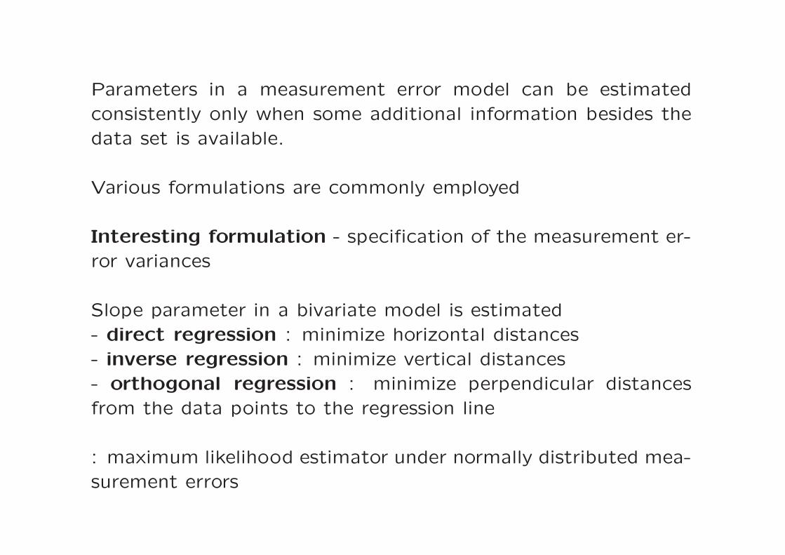
Parameters in a measurement error model can be estimated

consistently only when some additional information besides the

data set is available.

Various formulations are commonly employed

Interesting formulation - specification of the measurement er-

ror variances

Slope parameter in a bivariate model is estimated

- direct regression : minimize horizontal distances

- inverse regression : minimize vertical distances

- orthogonal regression : minimize perpendicular distances

from the data points to the regression line

: maximum likelihood estimator under normally distributed mea-

surement errors

Alternative procedures

Received less attention in the literature of measurement error

models

• Technique of reduced major axis: Estimate slope pa-

rameter by geometric mean of direct and inverse regression

estimators;

see, e.g., Sokal and Rohlf (1981)

• Estimate slope parameter by the arithmetic mean of direct

and inverse regression estimators;

see, e.g., Aaronson, Bothum, Moutld, Huchra, Schommer

and Cornell (1986)

• Slope parameter is estimated by the slope of the line that

bisects the angle between the direct and inverse regression

lines;

see, e.g., Pierce and Tully (1988).

What is the performance of these estimators under measurement

error models?

Which estimator is better under what conditions?

Measurement errors are assumed to be normally distributed

In practice, such an assumption may not always hold true and

leads to invalid and erroneous statistical consequences.

What is the effect of departure from normality on the properties

of estimators?

Ultrastructural Model

Yj = α + βXj (j = 1,2, . . . , n)

yj = Yj + uj

xj = Xj + vj

Xj = mj + wj

Yj : true but unobserved values of study variables

Xj : true but unobserved values of explanatory variable

yj : observed values of study variable

xj : observed values of explanatory variable

uj and vj : associated measurement errors

wj : random error component

α : unknown intercept term

β : unknown slope parameter

Assume that Xj’s are random with possibly different means mj

but same variance

• When m1 = m2 = . . . = mn, ultrastructural model reduces

to structural form

• When wj = 0 ∀ j = 1,2, . . . , n, (σ2w = 0), ultrastructural

model reduces to functional form

• When vj = 0 ∀ j = 1,2, . . . , n, (σ2v = 0) [i.e., no measure-

ment errors in xj], ultrastructural model reduces to classical

regression model.

Ultrastructural Model: very general framework for measurement

error modelling

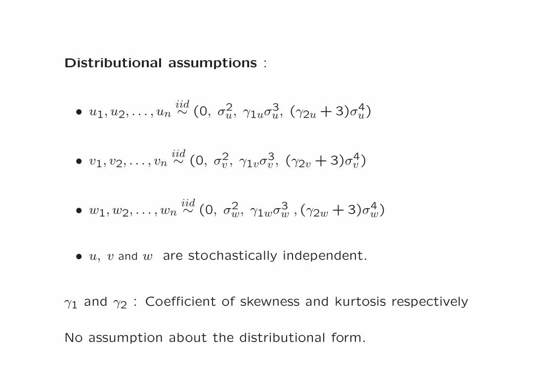
Distributional assumptions :

• u1, u2, . . . , uniid∼ (0, σ2

u, γ1uσ3u, (γ2u + 3)σ4

u)

• v1, v2, . . . , vniid∼ (0, σ2

v , γ1vσ3v , (γ2v + 3)σ4

v )

• w1, w2, . . . , wniid∼ (0, σ2

w, γ1wσ3w , (γ2w + 3)σ4

w)

• u, v and w are stochastically independent.

γ1 and γ2 : Coefficient of skewness and kurtosis respectively

No assumption about the distributional form.

Consistent estimation of α and β with n observations is possible

only when some additional information is available

z Measurement error variance σ2v is known

bd =sxy

sxx − σ2v

; sxx > σ2v

where

sxx =1

n

∑

(xj − x)2 , x =1

n

∑

xj ;

sxy =1

n

∑

(xj − x)(yj − y) , y =1

n

∑

yj

Direct regression estimator of slope parameter in the regres-

sion of yj on x∗j instead of xj where

x∗j = x +

(

1 −σ2

v

sxx

)

(xj − x)

z Measurement error variance σ2u is known

bi =syy − σ2

u

sxy; syy > σ2

u

where

syy =1

n

∑

(yj − y)2

Inverse regression estimator bi essentially arises from the re-

gression of xj on y∗j instead of yj where

y∗j = y +

(

1 −σ2

u

syy

)

(yj − y),

bd and bi utilizes the knowledge of only one error variance at a

time

z Estimator using the knowledge of both the error vari-

ances

bp = tp +

(

t2p +σ2

u

σ2v

)

12

; sxy 6= 0

where

tp =1

2sxy

(

syy −σ2

u

σ2v

sxx

)

Obtained by orthogonal regression

z Estimate β by reduced major axis

br = sign(sxy) (bdbi)12

: Geometric mean of bd and bi; [Sokal and Rohlf (1981)]

z Estimate β by

bm =1

2(bd + bi)

Mean of estimators bd and bi; [Aaronson et al. (1986)].

z Estimate β by

bb = tb + (t2b + 1)12 ; tb =

bdbi − 1

bd + bi

: Slope of line that bisects the angle between the two re-

gression lines specified by bd and bi; [Pierce and Tully (1988)].

Consistency of estimators :

Assume the variance of m1, m2, . . . , mn tends to a finite quantity

σ2m as n tends to infinity.

plim(bd − β) = 0

plim(bi − β) = 0

plim(bp − β) = 0

plim(br − β) = 0

plim(bm − β) = 0

plim(bb − β) = 0

bd, bi, bp, br, bm and bb are consistent for β.

Reliability ratios associated with study and explanatory vari-

ables are easily available or can be well estimated [Gleser (1992,

1993)].

Reliability ratio = Ratio of variances of true and observed values

Reliability ratios :

λx =σ2

m + σ2w

σ2m + σ2

w + σ2v

; 0 ≤ λx ≤ 1

λy =β2(σ2

m + σ2w)

β2(σ2m + σ2

w) + σ2u

; 0 ≤ λy ≤ 1

Express efficiency properties of estimators as a function of reli-

ability ratios

Helps in obtaining the conditions for the superiority of one esti-

mator over the other in terms of reliability ratios only.

Asymptotic relative variances

AsyRelV ar(bd) =1 − λx

λ2x

[λx + q + (1 − λx)(2 + γ2v)]

AsyRelV ar(bi) =1 − λx

λ2x

[

λx + q + q2(1 − λx)(2 + γ2u)]

AsyRelV ar(bp) =1 − λx

λ2x

[

λx + q +q2(1 − λx)

(q + 1)2(γ2u + γ2v)

]

AsyRelV ar(br) =(1 − λx)δ

4λ2x

AsyRelV ar(bm) =(1 − λx)δ

4λ2x

AsyRelV ar(bb) =(1 − λx)δ

λ2x

where

q =λx(1 − λy)

λy(1 − λx)and δ = 2[(1+λx)(1+q)+(1−λx)q

2]+(1−λx)(γ2v+q2γ2u)

• Skewness of the distributions of measurement errors has no

influence on the asymptotic variances of the estimators.

• Only the kurtosis shows its effect.

• Asymptotic variance for each estimator under normality of

errors could be quite different when the distributions depart

from normality.

• br and bm are equally efficient.

• br and bm are less efficient than bp when

(q − 1)[(3q + 1)γ2v − q2(q + 3)γ2u] < 2(q + 1)2(1 − q + q2).

– When q = 1, i.e., λx = λy, this condition is satisfied for

all kinds of error distributions.

– If λx 6= λy, the condition invariably holds true provided

that both the distributions of measurement errors are

mesokurtic or normal.

– Result remains true for non-normal distributions too when

γ2v < 0 (leptokurtic ) and γ2u > 0 (platykurtic).

– Both br and bm are asymptotically more efficient than bp

when the condition holds with an opposite inequality sign.

• br and bm are always better than bb.

• When both the error distributions are assumed to be nor-

mal, then bp is always more efficient than br, bm and bb, as

expected.

Monte Carlo Simulation:

To have an idea about the effect of departure from normal

distribution on the efficiency properties of the estimators-

1. normal distribution

2. skew-Normal distribution

3. t distribution

4. beta distribution and

5. Weibull distribution.

Sample sizes n = 25 (treated as small sample) and n = 43

(treated as large sample) are considered.

Empirical bias (EB) and empirical mean squared error (EMSE)

of bd, bi, bp, br, bm and bb are computed based on 5000 replica-

tions for different combinations of λx = 0.1,0.3,0.5,0.7,0.9

and λy = 0.1,0.3,0.5,0.7,0.9 under different distributions of

measurement errors.

The values EB and EMSE of these estimators are plotted

against λx and λy in a 3-dimensional surface plot.

Difference in two surface plots under two different distribu-

tions of measurement errors ⇒ behaviour of the estimator

depends on the distribution of measurement errors.

Bias(bb) with Normal Distribution (n = 43) Bias(bd) with t Distribution (n = 43)

Bias(bd) with Skew-Normal Distribution (n = 43) Bias(bd) with Beta Distribution (n = 43)

Empirical bias of bd when measurement errors follow

different distributions

MSE(bd) with Normal Distribution (n = 43) MSE(bd) with t Distribution (n = 43)

MSE(bd) with Skew-Normal Distribution (n = 43)

MSE(bd) with Beta Distribution (n = 43)

Empirical mse of bd when measurement errors follow

different distributions

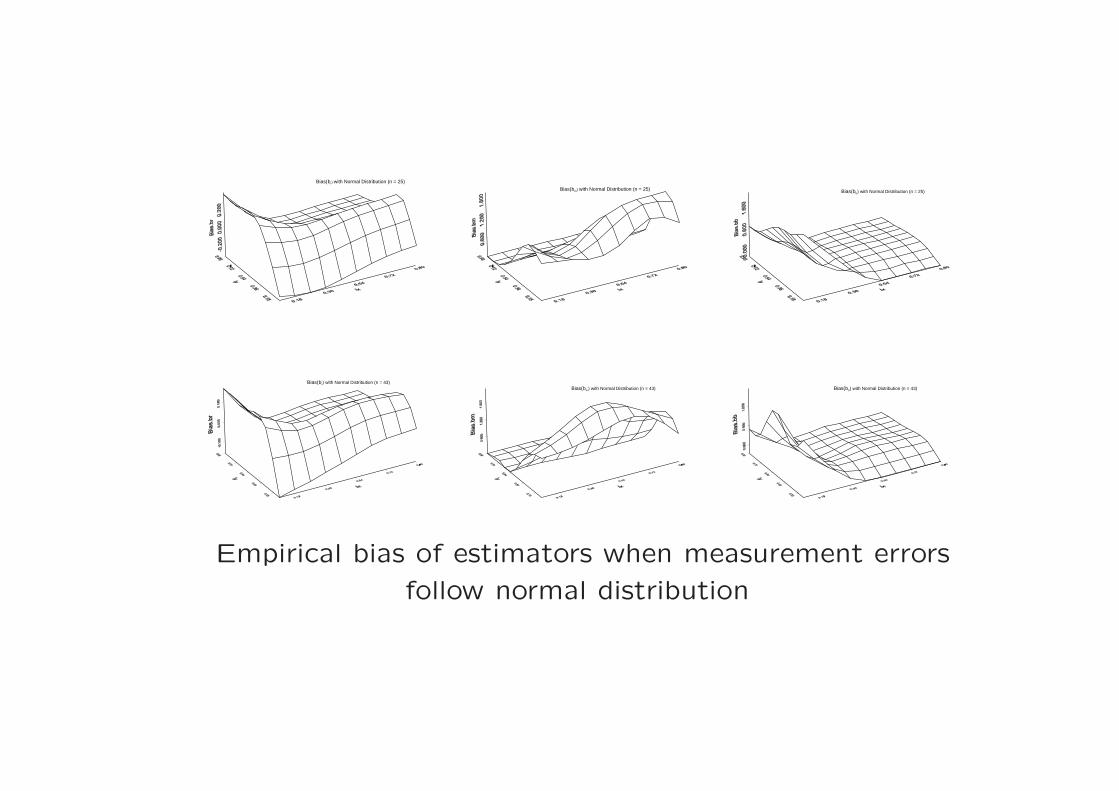
Bias(br) with Normal Distribution (n = 25)

Bias(bm) with Normal Distribution (n = 25) Bias(bb) with Normal Distribution (n = 25)

Bias(br) with Normal Distribution (n = 43)Bias(bm) with Normal Distribution (n = 43) Bias(bb) with Normal Distribution (n = 43)

Empirical bias of estimators when measurement errors

follow normal distribution

MSE(br) with Normal Distribution (n = 25)

MSE(bm) with Normal Distribution (n = 25) MSE(bb) with Normal Distribution (n = 25)

MSE(br) with Normal Distribution (n = 43) MSE(bm) with Normal Distribution (n = 43) MSE(bb) with Normal Distribution (n = 43)

Empirical mse of estimators when measurement errors

follow normal distribution

Empirical bias and empirical mean squared error of estima-tors under Normal distribution with n = 25

λx λy EB(bd) EMSE(bd) EB(bi) EMSE(bi) EB(bp) EMSE(bp) EB(br) EMSE(0.1 0.1 2.089 1172.2173 -1.3759 986.6908 3.4047 2515.2532 -0.30150.1 0.3 1.7396 421.1165 1.2588 6543.8844 7.1188 7082.3023 0.23040.1 0.5 0.6163 49.4849 1.0561 3011.413 15.193 63950.4496 0.39110.1 0.7 0.0841 1.3815 0.5237 2230.9995 23.5769 53226.1105 0.34840.1 0.9 0.0111 0.4415 2.1354 1731.3322 101.4696 2364682.359 0.36920.3 0.1 1.0035 3487.9245 0.0095 12390.1999 3.4205 46690.3197 -0.3530.3 0.3 2.2302 1139.6871 -0.049 689.9581 1.5118 933.892 0.1670.3 0.5 0.6255 32.431 0.1524 81.473 0.9368 367.1473 0.16860.3 0.7 0.0921 0.3203 0.1575 55.5964 1.03 584.3253 0.04050.3 0.9 0.0161 0.1262 0.0917 1.0878 0.4487 232.9447 0.010.5 0.1 0.9713 260.2454 -0.0198 563.1915 1.3962 504.9342 -0.26950.5 0.3 1.7528 225.9812 0.0442 46.6033 0.4372 36.7253 0.22860.5 0.5 0.7034 81.8598 0.0251 4.3178 0.1257 1.5329 0.12690.5 0.7 0.0864 0.1854 -0.0302 0.2743 0.03 0.3232 -0.00290.5 0.9 0.0137 0.0544 -0.0581 0.1496 0.0035 0.0519 -0.03810.7 0.1 1.6627 975.5491 0.49 1474.0067 1.7782 1106.7196 -0.17170.7 0.3 1.9329 349.1064 0.2131 29.5023 0.3467 23.0407 0.27880.7 0.5 0.5998 39.6491 0.027 0.4387 0.0623 0.1867 0.14250.7 0.7 0.0875 0.1319 -0.0119 0.0793 0.0229 0.056 0.02560.7 0.9 0.017 0.0285 -0.0308 0.0456 0.0061 0.0262 -0.01080.9 0.1 1.3506 417.5147 0.9993 5854.8029 2.1225 5206.1129 -0.12540.9 0.3 1.0239 199.6654 0.0509 103.5534 0.2089 6.0219 0.3120.9 0.5 0.6573 115.8942 0.0443 0.0878 0.0534 0.0878 0.17170.9 0.7 0.0891 0.106 0.0114 0.0309 0.0205 0.03 0.04410.9 0.9 0.0155 0.0122 -0.0044 0.0116 0.0049 0.0103 0.0049

Conclusions:

– The effect of non-normality is present and it affects the

performance of estimators. Kurtosis shows more effect

than skewness.

– No unique dominance of any estimator. It depend on the

choice of distribution of measurement errors and values

of reliability ratios.

– For lower values of λx and λy : More care is needed in

choosing the estimator.

Comparison of Normal and t surface plots

EB : Surface plots of all estimators are different

EMSE : Only br and bm have similar surface plots. Others

are different

Comparison of Normal and Skew-normal surface plots

EB : bd, bp and br have similar surface plots whereas bi, bb

and bm have different surface plots.

EMSE : bp has similar surface plots. Rest are different.

Comparison of Normal and Beta surface plots

EB and EMSE : All surface plots are different.

Normal Distribution:

– bd is more affected by λy.

– bi is more affected by λx.

– When λx and λy are low → br is better than other esti-

mators.

– When λx and λy are high → Performance of all estimators

stablize.

t Distribution:

– bd is more affected by λx.

– bi is more affected by λy.

– bd and bi are not good for lower values of λx and λy.

– When λx ≤ 0.5 and λy ≤ 0.5, bp and bm → high EB and

EMSE.

– When λx ≥ 0.5 and λy ≥ 0.5, br and bp → lower EB and

EMSE.

Skew-normal Distribution:

– bd, bp and bm → EB and EMSE are high for lower values

of λx and λy.

– bp is winner for most combinations of λx and λy.

– When λx is very low (say, 0.1) → Unstable performance

of all estimators.

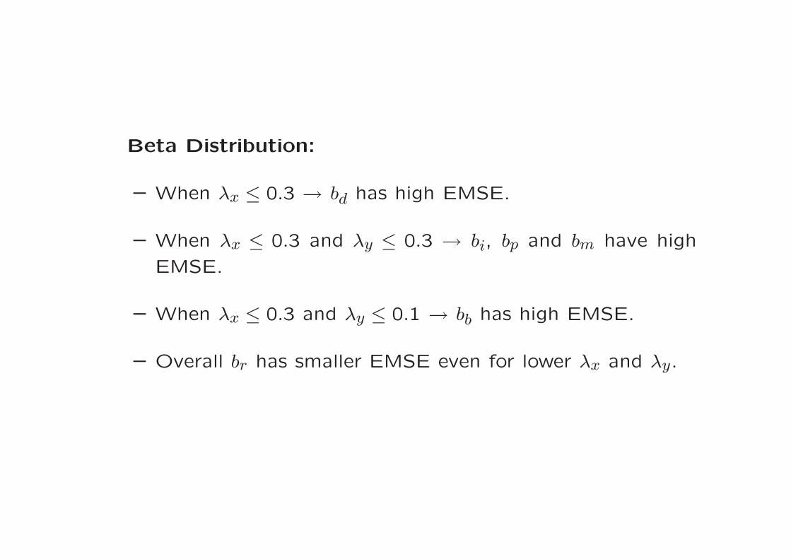
Beta Distribution:

– When λx ≤ 0.3 → bd has high EMSE.

– When λx ≤ 0.3 and λy ≤ 0.3 → bi, bp and bm have high

EMSE.

– When λx ≤ 0.3 and λy ≤ 0.1 → bb has high EMSE.

– Overall br has smaller EMSE even for lower λx and λy.

Weibull Distribution:

– Not good conditions.

– Extreme value presence.

– J- shaped curve

References

Aaronsom, M., G. Bothum, J. Moultd, J. Huchra, R.A.

Schommer and M.E. Cornell (1986): ‘A distance

scale from the infrared magnitude /HI velocity-width

relation. ν. distance moduli to 10 galaxy clusters, and

positive detection of bulk supercluster motion toward

the microwave anisotrophy’, Astrophysical Journal,

302, pp. 536-563.

Gleser, L.J. (1992): ‘The importance of assessing mea-

surement reliability in multivariate regression’, Jour-

nal of American Statistical Association, 87, 419, pp.

696-407.

Gleser, L.J. (1993): ‘Estimation of slope in linear

errors-in-variables regression models when the pre-

dictors have known reliability matrix’, Statistics and

Probability Letters, 17 (2), pp. 113-121.

Pierce, M.J. and R.B. Tully (1988): ‘Distances to

virgo and ursa major clusters and a determination

of H0’, Astrophysical Journal, 330, pp. 579-595.

Sokal, R.R. and F.J. Rohalf (1981): Biometry: The

principal and Practice of Statistics in Biological

Research, Second Edition, Freeman.