On the Economics of Higher Education in India, With ... papers/wp16.pdf · 1 On the Economics of...
28
1 On the Economics of Higher Education in India, With Special Reference to Women Sugeeta Upadhyay ∗ Gokhale Institute of Politics and Economics Pune 411 004 Maharashtra, India Abstract We investigate the role of economic factors in the enrolment decision at the higher education level in India. The study concludes that the rate of participation of women is in a disadvantaged position in the post-reform period. Women’s education has started to loose its importance as a determinant factor of economic development, rather, in the post-reform period, it has become the result of the latter. Relatively low ‘probability of getting job’, as well as, unfavourable prospect for ‘life time earnings’ of different female degree holders at the higher education level might have acted as a determinant factor in the enrolment decision for women in the post- reform period. Keywords: Higher Education, Human Capital Approach, Life Time Earnings, Probability of Getting Job, Age-Earning Profile, Rate of Return. JEL Classification: C23; D10; I20; I28; J01; O12 The saga of Indian economic development of the last half a century witnessed a lot of changes. India’s status has changed from a less developed country to that of a developing one. But in the literature, serious criticism exists with regard to the measures taken up by the government of India, particularly in the social sector. The critics argue that since independence, the performance of India in the social sector has been far from satisfactory and more could have been achieved if a proper policy measure was adopted. As far as policy measures are concerned, the measures taken up in the education sector since 1990, like cost share financing (tution fees) in public universities or encouraging privatization, have important implications for the equity aspects of the higher educational system of the country (Tilak 2004). It is in this background that the present study attempts to explore the relative picture of the higher education system in the pre and post-reform India, especially, in terms of the participation of women in higher education. We consider the higher education as university, as well as, college level education and estimate students’ participation in terms of the student enrolment based on the secondary data. In their pioneering work, Blaug, Layard and Woodhall (1969) observed that, in India, when students finish/leave their studies, many remain unemployed, and the number of these ∗ I gratefully acknowledge the long discussions, unstinted continuous support and efforts of Professor Arup Maharatna in the writing of this paper. Thanks are due for constructive comments as well as editorial efforts towards making the manuscript read better to my colleagues K.S. Hari, Sangeeta Shroff and S.N. Tripathi. I want to express my feelings of immense debt to all staff members of the Dhananjayarao Gadgil Library, Pune for their unconditional wonderful cooperation. And finally, the usual disclaimer applies.
Transcript of On the Economics of Higher Education in India, With ... papers/wp16.pdf · 1 On the Economics of...

1
On the Economics of Higher Education in India, With Special Reference to Women
Sugeeta Upadhyay∗
Gokhale Institute of Politics and Economics
Pune 411 004 Maharashtra, India
Abstract
We investigate the role of economic factors in the enrolment decision at the higher education level in India. The study concludes that the rate of participation of women is in a disadvantaged position in the post-reform period. Women’s education has started to loose its importance as a determinant factor of economic development, rather, in the post-reform period, it has become the result of the latter. Relatively low ‘probability of getting job’, as well as, unfavourable prospect for ‘life time earnings’ of different female degree holders at the higher education level might have acted as a determinant factor in the enrolment decision for women in the post-reform period.
Keywords: Higher Education, Human Capital Approach, Life Time Earnings, Probability of Getting Job, Age-Earning Profile, Rate of Return. JEL Classification: C23; D10; I20; I28; J01; O12 The saga of Indian economic development of the last half a century witnessed a lot of changes. India’s status has changed from a less developed country to that of a developing one. But in the literature, serious criticism exists with regard to the measures taken up by the government of India, particularly in the social sector. The critics argue that since independence, the performance of India in the social sector has been far from satisfactory and more could have been achieved if a proper policy measure was adopted. As far as policy measures are concerned, the measures taken up in the education sector since 1990, like cost share financing (tution fees) in public universities or encouraging privatization, have important implications for the equity aspects of the higher educational system of the country (Tilak 2004). It is in this background that the present study attempts to explore the relative picture of the higher education system in the pre and post-reform India, especially, in terms of the participation of women in higher education. We consider the higher education as university, as well as, college level education and estimate students’ participation in terms of the student enrolment based on the secondary data. In their pioneering work, Blaug, Layard and Woodhall (1969) observed that, in India, when students finish/leave their studies, many remain unemployed, and the number of these
∗ I gratefully acknowledge the long discussions, unstinted continuous support and efforts of Professor Arup Maharatna in the writing of this paper. Thanks are due for constructive comments as well as editorial efforts towards making the manuscript read better to my colleagues K.S. Hari, Sangeeta Shroff and S.N. Tripathi. I want to express my feelings of immense debt to all staff members of the Dhananjayarao Gadgil Library, Pune for their unconditional wonderful cooperation. And finally, the usual disclaimer applies.

2
‘educated unemployed’ (secondary school matriculation or above) increases annually. In another study, Psacharapoulos (1973) pointed out that the university enrolment in India was three times more than that of in Great Britain and about equal to that in Western Europe, excluding France. It is statistics like these that prompts observations such as, ‘The relatively high incidence of unemployment among the educated points up the economic waste involved in using scarce resources to educate and train young people….’ (Malenbaum 1957) or ‘continuing unemployment of the educated suggests that expenditure on education is not giving a positive return’ (Rao 1966). Therefore, some scholars expressed serious reservations about economic justification of the further expansion of the Indian higher education system. However, in reality, the Gross Enrolment Ratio (GER) has never been too high for India to support such a view. By definition, GER is the total enrolment of students in a given level of education, regardless of age, expressed as the percentage of the corresponding eligible official age-group population in a given school year. The ratio touched 11.58 for boys and 8.17 for girls and 9.97 for total population of the corresponding age group in recent years (Central Advisory Board of Education 2005). It may be a high ratio compared to some less developed countries, but not high as compared to the developed ones. Also, it would seem relatively ordinary in comparison with the target set by the Government of India from time to time. There is also a possibility that the overall estimate is misleading. First of all, the ratio includes many students who are over aged. Secondly, a sizeable percentage of them do not progress to higher level without either having to drop out or repeat. Thus, on an average, the overall figure is inflated by the number of over aged students and is unreflective of student wastage. In spite of these possibilities of overestimation, GER for women in India had never gone beyond eight per cent (Education in India, MHRD, various years) of the corresponding age group population. Education at the higher level in an economy is crucial to economic development simply because much of the possibilities for sustained growth in the medium and long-run depend on the extent to which the economy can develop and utilize high level human capital. This capital is essential for the organisation and innovation required in today’s global information economy. In addition, in the Indian case, it is even more pertinent since every year, a large number of student’s complete secondary education. Further, the Indian middle class keeps expanding rapidly whereas the land-based economic system is on the decline. As a result of all these, the importance of higher education is ever increasing. Hence, the state of the nation’s higher education system in terms of male and female participation is an issue of serious concern, especially considering the importance of inclusive growth of a country. In the literature on women studies and in the economics of education, substantial amount of work have been carried out at the international, as well as, national level on women’s education. Mention may be made of Cohen (1971), Gwartney (1972), Gadgil (1965), McNully (1967), Sheddy (1983), et al. These studies provide significant insight in to the different and varied economic benefits of women’s education in a society, not only in terms of income generation and increasing welfare but also in terms of developing a better quality of new generation. Sending kids to school today affects the cognitive achievements of children and grandchildren. Individuals benefit culturally and physically from increased access to health and welfare resources. The society at large benefits because of the diminishing costs of diffusing information, the potential acceptance of family planning and other social changes. If such benefits could be expressed in quantitative terms, the measure of overall benefits would increase many times at no additional cost, reinforcing the importance of women’s education in a society.

3
In the Indian history, there is evidence of well-educated women in ancient India, but records of a system of organized education accessible to girls during those days are not available. A regular education system for the girls of all classes probably did not exist in earlier times. In modern India, as per government reports (Education in India, MHRD) the total number of women enrolled for higher education in the country was only 264 in 1901. The government of India on October 1, 1919 reiterated the policy on women’s education. In 1925 the National Council of Women was established. The first All-India Women’s Education Conference was held in 1928. In 1944 the ‘Plan of Post-War Educational Development in India’ was prepared under the auspices of the Central Advisory Board of Education. It envisaged, for the first time a comprehensive national pattern of education from the primary to the university level and recommended several far reaching measures of reform in the education system. On record, the women enrolment in 1947-1948 were about 22,000 at higher level which was slightly less than 10 per cent of the total university population of that period. This figure increased to slightly more than 46,000 in 1950-1951 (Education in India, MHRD). Moreover, in the Sixth Plan women’s education was included as one of the major programme under women and development scheme. But in the course of all these efforts, the parity between men and women enrolment has never been achieved. In spite of the fact that it has been considered as one of the major goals by the authorities while preparing reports, namely, University Education Commission 1948-1949, The Education Commission 1964-1966 or National Policy on Education 1986. However, as far as educational policies are concerned, during the pre-reform period, the study by Psacharopoulos (1973) showed that the amount of physical capital per capita invested in India was 16 per cent more than in South Korea, but the amount of education capital invested per capita was 84 per cent less than South Africa (Table 1). Table 1: Educational and Physical Capital/ Member of the Labor Force by Country
Country Educational Capital (US$) Physical Capital (US$) Educational Capital as a % of physical capital/ Country (%)
United States 12,296 28,045 44
New Zealand 5,745 17,270 33
Great Britain 3,630 12,320 29
Israel 2,210 13,922 16
Chile 877 4,423 20
Greece 423 4,003 11
Mexico 410 4,040 10
South Korea 403 1,008 40
Philippines 290 3,446 8
Ghana 181 1,236 15
Kenya 157 920 17
Nigeria 88 697 13
Uganda 88 539 16
India 66 1,197 6
Source: Psacharopoulos, 1973: Tables E.1 and E.2 and 6.4. Taken from, “World Bank Staff Working Paper”, 1979, No. 327. Another example is that India invests 64 per cent less per capita in education than one of the less developed countries like Ghana. As a result, prior to reform only 0.6 per cent of India’s labor force were having post secondary education. From Table 2, it is clear that, this is very low compared to similar estimates available from other countries.

4
Table 2: Education Attainments of the Labor Force in 1969, by Country Country Less than primary
schooling Primary schooling Primary plus secondary schooling
Primary & secondary plus post-secondary schooling
United States - 35.6 45.2 19.2 Canada - 40.5 50.7 8.9 Great Britain - 54.6 35.0 10.4 Norway - 64.9 31.0 4.1 Greece - 89.2 7.9 2.9 Japan - 70.4 23.0 6.6 Israel 8.9 50.7 30.0 10.4 Colombia 12.7 64.7 20.3 2.2 Philippines 16.9 62.8 14.1 6.3 Turkey 19.3 62.3 14.3 4.1 Mexico 38.0 52.2 7.1 2.6 South Korea 44.9 39.3 13.4 2.4 Brazil 48.2 48.5 2.7 0.5 Uganda 66.5 30.9 2.5 0.1 Kenya 76.8 20.2 2.7 0.3 Ghana 81.6 16.5 1.5 0.3 Nigeria 90.0 8.5 1.3 0.2 India 90.0 7.3 2.2 0.6
Source: Psacharopoulos, 1973: Tables E.1. Taken from, “World Bank Staff Working Paper”, 1979, No.327. Thus even during pre-reform era, reduction in educated unemployment rate, as well as, a more rapid increase in the level of educated workforce has remained a dream largely unfulfilled. It is against this background, the higher education system (rather the whole education system) in India was drastically reformed with the introduction of New Economic Policy in 1991. This policy mainly advocates reduction of public expenditure and encourages privatization especially of higher education. In the pre-reform period, it was argued that, like in primary and secondary education, charging fees to cover the costs of higher education, which is much more expensive, would produce underinvestment due to imperfect capital markets. In the post-reform era, the economy has allowed higher education to become privatized. However, the way the country has made this shift or allowed it to happen has assumed important implications on the enrolment decision at the higher level. In the post-reform period even though many new schools and universities have been started, India targets to invest only six per cent of its national income in education following the suggestion made by Kothari Commission in 1964-1966. Moreover, recent budget studies assert that in practice only 3.8 per cent of GNP was spent by India on education in the year 2004, which is much less than the six per cent of the target rate. The post-reform employment estimate reveals that at the all-India level, among the rural female graduates, the worker-population ratio in the year 1993-1994 (which was 366) has declined at about six percentage points in 1999-2000 and then increased to 345 in 2004-2005. In urban areas, among the graduates and above, there was a decline in the ratio of about two percentage points for males in the consecutive periods, and for females, a decline of about three percentage points between 1993-1994 and 1999-2000 followed by an increase of nearly two percentage points between 1999-2000 and 2004-2005 (NSSO, 61st round, September, 2006). As an impact of all these, we want to explore the comparative situation of student enrolment in the pre, as well as, post-reform era at higher level. We consider the fact that when expenditure in education is considered as investment, while the phenomena ‘educated unemployed’ remains skewed towards women, the decision to invest on women’s higher education does get affected adversely. This hypothesis is based on the facts that investment in higher education is expected to be highly influenced by at least two important parameters
5
namely the ‘probability of getting job’ and the ‘life-time earnings’. In India, both of these two parameters are less for educated women than their male counterparts. Tilak (1987) in his study based on sample survey found that if the labour force participation rates for women and men were similar, the returns to women’s education would be higher to men’s education. He prescribed the probable reason as the costs of women’s education, private, as well as, social, are relatively lower. Hence, despite lower average earnings, the returns for women are higher compared to men. Duraisamy and Duraisamy (1995) using a large survey data, namely, the Degree Holders and Technical Personnel Survey, 1981, suggest that, in terms of the private rate of return to higher education in India, investment in women’s education is economically more profitable compared to men’s education in all the streams of education. This finding is, however, subject to the caveat that no adjustment is made for non-participation and sample selection bias which may change the return to women’s education. Kingdon and Unni (2001) used state-wide representative household data from two large states-Madhya Pradesh and Tamil Nadu-collected by the NSS Fourth Quinquennial Survey of Employment and Unemployment during 1987-1988 (43rd Round). The findings of their study also suggest that women’s returns to education are significantly higher than men’s; each extra year of schooling raising women’s wages (or productivity) by about 10 per cent and men’s by about eight per cent. They conclude women do not face poorer economic incentives to invest in schooling than men, although the conclusion may not be robust to the inclusion of family background in the analysis. All the above mentioned studies failed to explain the wide disparity in male-female enrolment in higher education. In the present study, we argue that for females having the same degree, the ‘probability of getting job’, as well as, the ‘life time earnings’ from higher education were always lower than male in the pre-reform period. This argument is based on the all-India level data from the Census of India. It is assumed that these factors are likely to influence women’s enrolment decision at the higher level in the post-reform period too. Therefore, it is possible that measures like privatization in the post-reform period may not help to increase the enrolment for higher education of women as compared to their male counterparts. The rest of the study is organized as follows. In the first section returns from different levels/streams of higher education have been estimated as an important determinant factor of enrolment at the higher level education in the pre-reform period. In the second section we discuss enrolment at higher level education with the help of some selected explanatory variables in the post-reform period too. We conclude the study in the third section by observing the fact that higher education in terms of rate of participation of women is in a disadvantaged position in the post-reform period compared to the earlier one. I. A Gender-Based Comparative Analysis of Returns to Higher Education in Pre-Reform India It is a known fact that countries are interested in raising the average level of education of their population because it will improve nation’s productivity, economic growth and help in reducing poverty and inequality. Similarly, from the individual’s point of view, higher secondary degree holders are encouraged to enroll in higher education only when the expected returns to higher education are higher. Returns to education are popularly measured via income payments. A study conducted on British and American data concluded that at

6
every level of education, mean or median earnings of women are lower than men with same level of education (Women’s Bureau, 1969). Several quantitative studies are available on the rate of return to education for India. Notable among them are Harberger (1965), Husain (1967), Nalla Gouden (1967), Blaug (1972), Psacharopoulos (1973), Shortlidge (1974), Pandit(1972), Duraisamy and Duraisamy (1995), Kingdon and Unni (2001)1. Major findings of these studies are summarized in Table 3. Table 3: Differential Rates of Return# to Investment in Education in India
Social Rates of Return College Source
Primary Middle School Matriculation BA Engin.
Blaug (1972) 13.7 12.4 9.1 7.4* Psacharopoulos (1973) 20.2 16.8¤* 12.7* Harberger (1965) - 10¤* 16.3* Nalla Gounden (1967) 16.8 11.8 10.2 7.0 9.8 Kothari (1967 & 1970) - - 20 14 25.0 Husain (1967) - - 37.0¤ 4 Pandit (1967) 13.4 15.5 - 10.7 Shortlidge (1974) - - - 10.3** Average 16.0 13.3 13.1 10.3 17.4 Tilak (1987) Unadjusted estimates
Tilak (1987) Adjusted estimates
Rao & Dutta (1989) Duraisamy (2002) Unadjuated estimates
Duraisamy (2002) Adjuated estimates
Private Rates of Return College Source
Primary Middle School Matriculation BA Engin.
Blaug (1972) 16.5 14 10.4 8.7* Psacharopoulos (1973) 24.7 19.2¤* 14.3* Harberger (1965) Nalla Gounden (1967) Kothari (1967 & 1970) 10.0 25.0 Husain (1967) - - 48¤ 12.0 Pandit (1967) 17.3 18.8 - - Shortlidge (1974) - - - 16.2** Average 19.5 17.3 10.4 12.2 25.0 Tilak (1987) Unadjusted estimates 33.4 25.0 19.8 13.2
Tilak (1987) Adjusted estimates 7.82 8.54 negative 6.82
Rao & Dutta (1989) 5.3 5.07 Duraisamy (2002) Unadjuated estimates 7.9 7.4 17.3 11.7 14.6
Duraisamy (2002) Adjuated estimates 7.8 7.4 17.7 12.7 16.6
# Differential Rates of Return refer to the differential benefits of each educational qualification over the lifetime earnings of unqualified school leavers of a given base age. 172− Type of degree unspecified. ¤ Rate of total return, i.e. matriculation over zero years of schooling. ¤* Level of secondary unspecified. ** B. Sc. Agriculture over matriculation. Source: World Bank Staff Working Paper, 1979, No.327, Tilak (1987), Rao and Datta (1989), Duraisamy (2000).
7
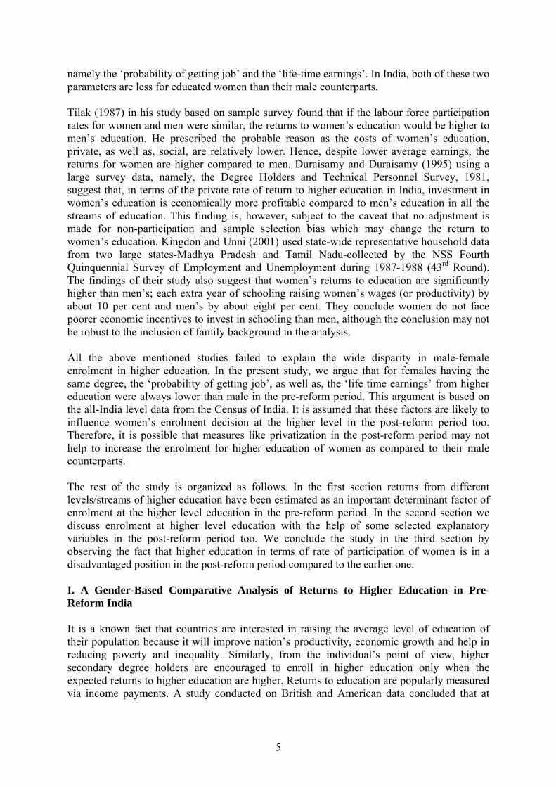
Most of the studies mentioned above were silent on the estimation of returns to education for women. A major problem that has been highlighted in these studies is that the rate of return measure ‘benefits’ solely in terms of earnings from market work and a large part of women’s work takes place outside the market. Further, information on the ‘age-earning profiles’, which is the mean earnings of cohorts with different levels or years of education are not available. Thus, in order to get a comparative picture of returns to education for male and female at the all-India level of the pre-liberalisation period, we attempt a separate study using data from the Census of India. Here two important points should be made clear. Firstly, the difficulty in carrying out the same exercise for the post-reform period, mainly due to non-availability of reliable secondary data on age-earning profiles of educated persons at the all-India level. Secondly, there is a rationale behind carrying out the exercise for pre-reform period to capture changes in the skill requirement in the labour market, especially, software skill, which barely existed in the pre-reform period. Further, it is believed that there has been a marked increase in wages in the post-reform period, which will increase the opportunity cost for women. But, results from the secondary data at the all-India level (NSSO, 61st round) given in Figure 1 and 2 confirms that the position of graduate and above degree holder female in terms of average earnings, as well as, work participation is still substantially lower as compared to their male counterpart with the same qualification. Figure 1: Unemployment rate (per 1000 persons in the labour force) among the youth (15-29 years) according to usual status (adjusted) during 2004-2005
Source: NSSO, 61st Round on Employment and Unemployment Situation in India, 2004-2005.
0
50
100
150
200
250
Rural Male Rural Female Urban Male Urban Female
Sex and Sector
UR
(per
100
0 pe
rson
s in
the
labo
ur fo
rce)
15-19
20-24
25-29
15-29
8
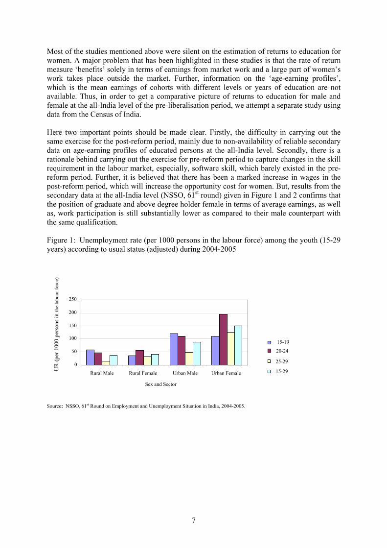
Figure 2: Unemployment rate (per 1000 persons in the labour force) according to usual status (adjusted) for the persons of age 15 years and above with different general educational level during 2004-2005
Source: NSSO, 61st Round on Employment and Unemployment Situation in India, 2004-2005. Table 4, highlights that considering ‘Regular Wage Salary’ (RWS) workers, the structure of wage differentials by gender, rural-urban location and by enterprise type, by and large follows a priori expectations. Adult wages are higher for males than females and higher in urban areas compared to rural areas. Wages of the RWS workers in the corporate segment are higher than those in proprietary/partnership enterprises in the factory sector, whereas wages in the latter are higher than those in other proprietary/partnership enterprises. Within the corporate segment, the average daily earnings are higher in government/public sector relative to those in public/private limited companies, which are generally higher (except for rural females) than the average daily earnings of RWS workers in cooperatives/trust/non-profit institutions. Moreover, what is important is that except in respect of female workers in public/private limited companies, gender-differentials, for a given enterprise type, are greater than the rural-urban differentials for a given gender. Table 4: Average Daily Earnings of Regular Wage Salary (RWS) Workers in Non-Agricultural Activities by Gender, Rural-Urban Location and by Type of Enterprise: All-India, 2004-2005 (Average Daily Earnings of Adult (15-59) Workers Rs. (0.00))
Enterprise Type Rural Males Rural Females Urban Males Urban Females
1-4 Non-factory 68.20 36.79 87.97 41.64
1-4 Factory 91.76 51.32 124.74 80.08
5 238.60 136.22 324.00 277.37
6 176.41 59.11 271.94 225.41
7 160.00 93.78 178.32 171.48
5-7 220.06 120.93 300.09 250.54
Note: 1) Computed from unit record data; 2) Enterprise type 1-4 non-factory :proprietary/partnership enterprises excluding such enterprises engaged in manufacturing using electrical and employing 10 or more workers i.e. those in the factory sector; 3) Enterprise type 1-4 factory; proprietary/ partnership enterprises engaged in manufacturing in the factory sector. 4) Enterprise type 5: Government/public sector. 5) Enterprise type 6: Public/private limited company; 6) Enterprise type; 7) Cooperative society/trust/other non-profit institutions. Source: NSSO, 61st Round on Employment and Unemployment Situation in India, 2004-2005.
0
50
100
150
200
250
300
Rural Male Rural Female Urban Male Urban Female
Sector and Sex
UR
(per
100
0 pe
rson
s in
the
labo
ur fo
rce)
Not Literate Literate and upto primary
Middle
Secondary Higher Secondary Diploma/Certificate course
Graduate & above Secondary and above

9
We now explain the observation in detail. The finding confirms that the difference in average earnings is statistically significant between male and female both for rural and urban area (Table 5, Table 6). Table 5: Average wage/salary earnings (Rs. 0.00) per day received by regular wage/salaried employees (31, 71 & 72) of age 15-59 years by industry of work and broad education category
Education Category (All-India Level) Secondary & Higher
Secondary Diploma/ Certificate Graduate and above Sector of Work (Industry division/group) Rural Male
Rural Female
Rural Male
Rural Female
Rural Male
Rural Female
Agriculture (01-05) 149.40 134.61 96.26 334.41 200.33 105.32 Mining & quarrying (10-14) 323.41 83.29 273.00 33.00 341.46 0.00 Manufacturing (15-22) 103.40 47.26 253.94 144.41 160.67 89.21 Manufacturing (23-37) 109.43 62.12 145.03 120.50 534.81 219.58 Electricity, gas and water (40-41) 260.51 290.91 353.35 327.30 306.55 111.91 Construction (45) 111.08 101.70 186.29 249.29 223.09 136.09 Trade (50-55) 86.57 67.51 96.85 109.16 108.34 136.45 Transport and storage etc. (60-64) 138.45 105.32 218.00 0.00 235.17 256.22 Services (65-74) 193.12 89.95 203.26 185.76 278.29 157.28 Services (75-93) 197.20 105.74 239.65 210.96 256.93 174.18 Private hhs. withemp. persons (95) 88.14 54.90 42.86 0.00 137.67 0.00 Others 0.00 - 0.00 - 250.00 - Non-agricultural (10-99) 158.29 99.35 215.35 200.37 271.30 173.16 All 158.04 100.19 214.38 200.40 270.02 172.70 t-stat* 1.75 0.74 3.58 P-Value 0.05 0.23 0.00
* Where, Ho (μ1 =μ2), H1 (μ1 ≠μ2 ). Source: NSSO, 61st Round on Employment and Unemployment Situations in India, 2004-2005. Table 6: Average wage/salary earnings (Rs. 0.00) per day received by regular wage/salaried employees (31, 71 & 72) of age 15-59 years by industry of work and broad education category
Education Category (All-India Level) Secondary & Higher
Secondary Diploma/ Certificate Graduate and above Sector of Work (Industry division/group)
Urban Male Urban Female Urban Male Urban Female Urban Male Urban FemaleAgriculture (01-05) 182.06 74.20 0.00 266.71 237.37 225.56 Mining & quarrying (10-14) 348.64 714.29 343.22 212.36 806.61 351.30 Manufacturing (15-22) 122.10 70.71 199.92 54.81 218.85 235.10 Manufacturing (23-37) 176.79 113.24 239.36 238.87 362.06 219.39 Electricity, gas and water (40-41) 325.56 240.48 384.04 273.17 523.53 422.72 Construction (45) 106.45 147.59 259.93 127.07 376.45 253.59 Trade (50-55) 112.21 95.07 146.67 88.97 208.97 204.85 Transport and storage etc. (60-64) 211.92 228.99 341.87 138.83 361.17 414.48 Services (65-74) 174.19 131.04 287.73 356.09 501.69 372.60 Services (75-93) 239.72 186.33 309.62 236.30 345.63 247.12 Private hhs. with emp. persons (95) 62.95 51.67 0.00 34.23 164.08 67.61 Others 134.00 66.71 0.00 0.00 0.00 0.00 Non-agricultural (10-99) 182.59 150.64 274.87 237.02 367.06 269.29 All 182.58 150.41 274.87 237.02 366.76 269.17 t-stat* 0.16 0.83 3.58 P-Value 0.44 0.21 0.00
* Where, Ho (μ1 =μ2), H1 (μ1 ≠μ2 ). Source: NSSO, 61st Round on Employment and Unemployment Situations in India, 2004-2005.

10
Thus, the disparity between male and female educated personnel regarding average earnings or work participation rate are a common feature both in the pre and post-reform period. Hence, we assume that decisions taken by the parents for their children’s higher education may be based more or less on the same assumptions as in the pre-reform period. Hence, the present study is different from those of the earlier works not only in terms of coverage but also with respect to the reference period, the nature and size of data and more importantly differences in the methodology2. The important source of methodological difference among all the studies are the number and magnitude of adjustment factors used for analysis. Mention may be made of a few of them. Firstly, though the debate on the adjustment for ability itself is inconclusive, Nallagoundan (1967), Blaug et al. (1969), Pandit (1972) and Goel (1975) have assumed all the earnings differentials cannot be attributed to education only. Many authors, mostly American, have tried to identify the factor and called it as ‘alpha’ factor-that coefficient which expresses the proportion of the observed differentials which can be directly attributable to extra education, such that 0<α<1. The standard expression of which is
100)()()( 333222111 ×ΝΝΡ
−+−+−=
fyxfyxfyxe ααα
where e stands for the share of education in the Net National Product (NNP). 1α , 2α , 3α denote the value of the alpha coefficient for different levels of education. The average earnings of persons educated up to the primary, secondary and higher levels in a given year is indicated by 1x , 2x , 3x .Their number in the labour force of the country during the year by 1f , 2f , 3f respectively. The average earnings of persons with no formal education by y. A number of studies have been made in the USA to determine the alpha coefficient (Becker, G. 1957; Denison, E.F. et al., 1962). But empirical evidence on the order of influence of the non-educational or ability factor on earnings is not systematic. So in literature, adjustment for ability has been made either by assuming a value for the alpha coefficient or by estimating it with the help of the multiple regression analysis using an indicator of ability as one of the explanatory variable besides education. But since the latter method can be adopted only if one has large samples to deal with and sufficiently good indicators of ability, one is left with only option of arbitrarily assuming a certain reasonable value for the coefficient. Hence, the values of the coefficients varies arbitrarily from one study to another. Secondly, Blaug et al. (1969), Goel (1975) and Pandit (1972) considered different growth rate in their estimation of returns to education. In order to estimate the rates of return to education, one requires data on lifetime earnings of individuals by age and educational levels. But time-series data on age-education earnings profile are not available even in advanced countries. Most studies are therefore, based on cross-sectiona data collected through national or regional census or sample surveys (Eckaus et al. 1974). The cross-section age-earnings profiles, however, do not truly represent the lifetime earnings profiles. The lifetime earnings profiles are, therefore, obtained by inflating the cross-section earnings profile by the rate of growth of individual incomes. In Indian case, Blaug, et al. and Goel assumed a secular long-term growth rate of two per cent; Pandit criticised it to be on the higher side and assumed a rate of 1.5 per cent, based on long-term economic growth in India between 1860 and 1962.
11
Thirdly, premature death of educated individuals results in a loss in the potential benefits of education. But the age-specific mortality rates by educational levels for different groups of population are required for estimating this. In the absence of such data, age-specific mortality rates are used with the probability of a wide margin of errors. Besides, educated individuals having particularly graduate level education or above, belong to a relatively higher socio-economic stratum, whose class-specific mortality can be expected to be lower than those from others, because of differences in the standard of living. Thus, though the general assumption is that mortality rates would not affect the rates of return to education significantly, Kothari (1966), Husain (1967) and Pandit (1972) used different sources like general life-tables or data provided by the Life Insurance Corporation of India to adjust their estimates for mortality. Fourthly, people usually remain unemployed for some time immediately after completing their education. Several studies have confirmed that in 1956 in India, only 27,000 university graduates and 2,18,000 secondary school graduates had registered their names as unemployed but by 1961, 56,000 and 5,34,000 were registered; and by 1966, 94,000 and 8,24,000 (Blaug, et al. 1969) whereas, by 1972, the number of registered unemployed had climbed to 3.3 million (UNESCO 1977). Moreover, in urban areas an additional 30 per cent were not working but did not register (Blaug, et al. 1969). In any case, while carrying out his study Harberger (1965) assumed 100 per cent employment rate for all other than primary school leavers while adjusting for the unemployment factor. Based on the Directorate General of Employment and Training surveys, Husain (1967) assumed an unemployment rate of 13 per cent for graduates, seven per cent for post graduates and zero for professional graduates. Blaug et al. assumed a waiting period of 6 months for graduates and on the basis of the National Sample Survey data Pandit (1972) assumed this waiting period as 11 months for higher educated persons. Nallagoundan (1967) and Kothari (1966) recognized the problem of unemployment, though did not consider this factor in their estimation. In the present study, many of the above mentioned adjustments could not be done mainly due to lack of reliable secondary data at the all-India level. We, however, considered the ratio between persons employed and persons in the labour force separately for males and females. Labour force is defined as employed, self-employed, as well as, job seekers according to the different levels of education. In these estimation, those who were not interested in seeking jobs and were unemployed (home makers) have been excluded. This estimation is based on all India sample, with different educational backgrounds and with the average earnings from different level of education as a determinant of enrolment for that particular level of higher education. Hence, we have adjusted our findings by considering the condition of labour market or the rate of unemployment along with the returns to education in the pre-liberalisation period. The factual basis for such adjustment is that in real life, there is always a possibility that a student after receiving a particular level of education will remain unemployed. As a result, the participation for that particular level of education may be influenced by the fact of the zero or negative return after investing time, as well as, expenditure for getting that particular level of education. Hence, while considering the Indian higher education situation, in addition to the returns in terms of income payments to the training received, the enrolment at any particular stream of education is also associated with the ‘probability of getting job’ after completion of that particular training. However, the value of education is not just a function of the jobs that workers with more education can get in the labour market. More education of the labour force increases output in two ways: first, education improves the quality of labour as a factor of production and

12
permits technological development; and secondly it places human capital at the core of the economic process and assumes that the externalities generated by human capital are the source of self-sustaining economic growth process. Human capital not only produces higher productivity for more educated workers but for most other labour as well (Lucas 1988; Romer 1990). There does not exist a clear agreement amongst the economists as to what formulation describes or estimates the externalities best. We, therefore, do not consider that aspect in the present analysis. Our analysis on the basis of secondary data shows that the ‘probability of getting job’ for almost all qualification levels (excepting the other post graduate degree/diploma category) was lower for females than males during the period under consideration (Table 7). Table 7: Probability of Getting Job (Pr
*) By Different Educational Levels
Note: Pr* = LT / (LT+ LS), where, LT= Employed+Self-employed, LS= Job Seekers.
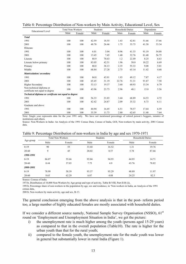
Source: Census, 1971, Series1, Part VII(i), Special Tables (G-1). Table 8 and 9 gives result for post-liberalisation period. Table 8 shows that in 1991 among ‘graduate and above’ degree holder non-workers, 70.57 per cent of females were associated with household duties. In 2001, the corresponding figures are 62.65 per cent. For males the percentage figures are 6.51 in 1991 and 2.80 in 2001. It, therefore, follows that even in the post-liberalisation period more than 50 per cent of the non-worker females with higher educational levels are associated with household duties. Obviously the percentage is negligible for males. In 1991, among male ‘graduate and above’ non-workers, 44.94 per cent were student; this figure came down to 35.39 per cent in 2001. For females, the percentage figures were as low as 16.45 in 1991 and 11.73 in 2001 respectively. But we must admit that the picture emerging from Table 8 is somewhat ambiguous since this does not give any age-specific distribution of non-workers. Table 9 gives the distribution of sample of 10,000 non-workers (males and females separately) for the year 1970-1971 and percentage distribution of non-workers by main activity, and sex for 1990-1991 and 2001. It is clear from Table 9 that in 1970-1971, of the total male non-workers, an overwhelming majority (more than 90 per cent) falls in the age group below 19 years. While for females this proportion is around 55 per cent. This indicates that more than nine per cent of the male non-workers are adult (20 years and above), while 45 per cent of the female non-workers belong to the same age group. In the year 1991, the percentage slightly came down to 8 for male and 37 for female but in 2001 it again increased to 9.65 for male and 62.29 for females. If infants and dependents are excluded, among the ‘student’ category of non-workers, majority (more than 90 per cent) belong to the younger age-group, 0-19 years. But a majority of female (78.82 per cent in 1991 and 82.5 per cent in 2001) non-workers belong to the adult group (20-60 years) and fall in the category of those doing ‘household duties’.
Educational Level
Doctorate Masters Degree Other PG Degree/ Diploma Bachelor Bachelor Equivalent Diploma Certificate
Male 93% 83% 71% 71% 75% 78% 67%
Female 80% 63% 72% 51% 60% 66% 58%
13
Table 8: Percentage Distribution of Non-workers by Main Activity, Educational Level, Sex Total Non-Workers Students Household Duties Dependents Educational Level
Male Female Male Female Male Female Male Female Total 1991 100 100 42.59 18.55 1.43 42.81 51.66 37.66 2001 100 100 48.70 26.46 1.75 35.75 41.58 33.34 Illiterate 1991 100 100 6.01 3.04 0.96 41.33 91.19 54.88 2001 100 100 13.45 7.45 1.40 32.76 81.48 56.75 Literate 100 100 88.9 70.43 1.2 22.49 8.25 6.63 Literate below primary 100 100 83.05 42.51 1.96 50.0 10.22 6.69 Primary 100 100 80.0 38.13 2.35 55.33 9.08 5.01 Middle 100 100 68.84 27.28 2.75 65.14 11.42 4.68 Matriculation/ secondary 1991 100 100 84.8 43.91 1.93 49.12 7.87 4.17 2001 100 100 65.45 31.19 22.76 51.31 91.87 7.58 Higher Secondary 100 100 53.13 19.37 3.68 60.93 15.34 6.79 Non-technical diploma or certificate not equal to degree 100 100 43.96 23.73 2.96 48.1 15.0 5.56
Technical diploma or certificate not equal to degree 1991 100 100 56.33 21.03 3.44 68.89 14.53 4.72 2001 100 100 42.42 24.87 2.09 35.32 8.73 6.11 Graduate and above 1991 100 100 44.94 16.45 6.51 70.57 17.64 6.59 2001 100 100 35.39 11.73 2.80 62.65 11.48 7.64
Note: Single year represents data for the year 1991 only. We have not mentioned percentage of retired person’s beggars, inmates of institutions and others. Source: Non-Workers in India: An Analysis of the 1991 Census Data, Census of India, GOI, Non-workers by main activity, 2001 Census data. Table 9: Percentage Distribution of non-workers in India by age and sex 1970-1971
Total Non-Workers Students Household Duties Age-group
Male Female Male Female Male Female
0-19 90 55 33.44 16.52 1.31 19.76 20-60 9 45 20.02 0.57 5.78 87.66
1990-1991 0-19 86.07 55.66 92.04 94.93 44.93 14.71 20-60 8.44 37.03 7.75 4.9 43.76 78.82
2000-2001 0-19 78.99 58.39 93.37 95.29 48.89 11.97 20-60 9.65 62.29 6.07 4.08 24.25 82.5
Source: Census of India. 1971b, Distribution of 10,000 Non-Workers by Age-group and type of activity, Table B-VIII, Part-II-B (ii), 1991b, Percentage share of non-workers in the population by age, sex and residence, in ‘Non-workers in India, an Analysis of the 1991 census data, 2001b, Non-workers by main activity, age and sex, B-13. The general conclusion emerging from the above analysis is that in the post- reform period too, a large number of highly educated females are mostly associated with household duties. If we consider a different source namely, National Sample Survey Organisation (NSSO), 61st round on ‘Employment and Unemployment Situation in India’, we get the picture:
i) the unemployment rate is much higher among the youth (persons aged 15-29 years) as compared to that in the overall population (Table10). The rate is higher for the urban youth than that for the rural youth;
ii) compared to the female youth, the unemployment rate for the male youth was lower in general but substantially lower in rural India (Figure 1).
14
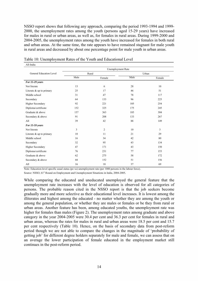
NSSO report shows that following any approach, comparing the period 1993-1994 and 1999-2000, the unemployment rates among the youth (persons aged 15-29 years) have increased for males in rural or urban areas, as well as, for females in rural areas. During 1999-2000 and 2004-2005, the unemployment rates among the youth have increased for females in both rural and urban areas. At the same time, the rate appears to have remained stagnant for male youth in rural areas and decreased by about one percentage point for male youth in urban areas. Table 10: Unemployment Rates of the Youth and Educational Level
All-India
Unemployment Rate
Rural Urban General Education Level Male Female Male Female
For 15-29 years Not literate 13 6 28 10 Literate & up to primary 25 17 46 51 Middle school 31 47 78 117 Secondary 64 133 96 225 Higher Secondary 92 221 105 254 Diploma/certificate 152 325 175 245 Graduate & above 157 363 185 304 Secondary & above 91 208 133 267 All 39 42 88 149
For 15-59 years Not literate 3 2 10 3 Literate & up to primary 10 11 21 29 Middle school 16 34 42 80 Secondary 32 95 43 134 Higher Secondary 47 171 43 150 Diploma/certificate 76 231 77 153 Graduate & above 62 275 58 172 Secondary & above 44 152 51 156 All 16 18 37 69
Note: Education-level specific usual status (ps+ss) unemployment rate (per 1000 persons in the labour force). Source: NSSO, 61st Round on Employment and Unemployment Situations in India, 2004-2005. While comparing the educated and uneducated unemployed the general feature that the unemployment rate increases with the level of education is observed for all categories of persons. The probable reason cited in the NSSO report is that the job seekers become gradually more and more selective as their educational level increases. It is lowest among the illiterates and highest among the educated - no matter whether they are among the youth or among the general population, or whether they are males or females or be they from rural or urban areas. Another feature has been, among educated youths, the unemployment rate was higher for females than males (Figure 2). The unemployment rates among graduate and above category in the year 2004-2005 were 30.4 per cent and 36.3 per cent for females in rural and urban areas, whereas the rates for males in rural and urban areas were 18.5 per cent and 15.7 per cent respectively (Table 10). Hence, on the basis of secondary data from post-reform period though we are not able to compare the changes in the magnitude of ‘probability of getting job’ for different degree holders separately for male and female, we can assess that on an average the lower participation of female educated in the employment market still continues in the post-reform period.
15
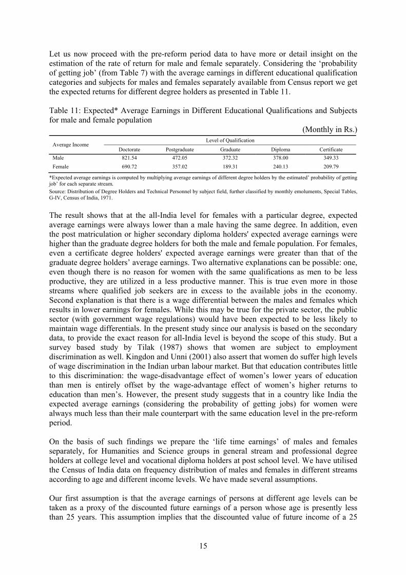
Let us now proceed with the pre-reform period data to have more or detail insight on the estimation of the rate of return for male and female separately. Considering the ‘probability of getting job’ (from Table 7) with the average earnings in different educational qualification categories and subjects for males and females separately available from Census report we get the expected returns for different degree holders as presented in Table 11. Table 11: Expected* Average Earnings in Different Educational Qualifications and Subjects for male and female population
(Monthly in Rs.) Level of Qualification
Average Income Doctorate Postgraduate Graduate Diploma Certificate
Male 821.54 472.05 372.32 378.00 349.33 Female 690.72 357.02 189.31 240.13 209.79
*Expected average earnings is computed by multiplying average earnings of different degree holders by the estimated’ probability of getting job’ for each separate stream. Source: Distribution of Degree Holders and Technical Personnel by subject field, further classified by monthly emoluments, Special Tables, G-IV, Census of India, 1971. The result shows that at the all-India level for females with a particular degree, expected average earnings were always lower than a male having the same degree. In addition, even the post matriculation or higher secondary diploma holders' expected average earnings were higher than the graduate degree holders for both the male and female population. For females, even a certificate degree holders' expected average earnings were greater than that of the graduate degree holders’ average earnings. Two alternative explanations can be possible: one, even though there is no reason for women with the same qualifications as men to be less productive, they are utilized in a less productive manner. This is true even more in those streams where qualified job seekers are in excess to the available jobs in the economy. Second explanation is that there is a wage differential between the males and females which results in lower earnings for females. While this may be true for the private sector, the public sector (with government wage regulations) would have been expected to be less likely to maintain wage differentials. In the present study since our analysis is based on the secondary data, to provide the exact reason for all-India level is beyond the scope of this study. But a survey based study by Tilak (1987) shows that women are subject to employment discrimination as well. Kingdon and Unni (2001) also assert that women do suffer high levels of wage discrimination in the Indian urban labour market. But that education contributes little to this discrimination: the wage-disadvantage effect of women’s lower years of education than men is entirely offset by the wage-advantage effect of women’s higher returns to education than men’s. However, the present study suggests that in a country like India the expected average earnings (considering the probability of getting jobs) for women were always much less than their male counterpart with the same education level in the pre-reform period. On the basis of such findings we prepare the ‘life time earnings’ of males and females separately, for Humanities and Science groups in general stream and professional degree holders at college level and vocational diploma holders at post school level. We have utilised the Census of India data on frequency distribution of males and females in different streams according to age and different income levels. We have made several assumptions. Our first assumption is that the average earnings of persons at different age levels can be taken as a proxy of the discounted future earnings of a person whose age is presently less than 25 years. This assumption implies that the discounted value of future income of a 25

16
years old person is equivalent to the average earnings of different persons with different ages at the same period. In fact the probable earnings of 25 years old person when he would be 55 years of age is expected to be much higher than the earnings of a person who is at present 55 years of age. Our second assumption is that, if enhancement of pay scales is made to make up for the increased general price level, then the purchasing power of the probable future income of a 25 year old person when he is of 55 years of age should be equal to the purchasing power of a person who is at present 55 years of age. Therefore, we may assume that the present value of the future income of a 25 years old person when he would be of 55 years of age will be exactly equal to the income of a person who is at present 55 years of age. The counter argument can be made of increase in the real income over the period as a substitute of constant purchasing power throughout the lifetime. Hence it is also necessary to consider the growth of real income in this calculation. But this growth of real income was negligible in the pre-reform period. For example, Blaug et al, (1972) and Goel (1965) assumed a secular long-term growth rate of two per cent; Pandit (1972) assumed a rate of 1.5 per cent, based on long-term economic growth in India between 1860 and 1962 in their estimation of return to education. However, by multiplying the life time earnings of all the different levels of education with the rate of growth of real income instead of considering constant purchasing power for the life time would not change the relative importance of different levels of earnings. Our findings have been expressed particularly in relative terms since our purpose is to compare between different streams of education instead of different levels. Thus, for all different ages discounted value of a 25 years old person’s future income can be assumed to be equal to the present income of different persons of different ages. This gives us future earnings of a person at different age levels. But since the person would get the income at different future dates our third assumption is that he must discount these values in order to evaluate the benefit at present. We have constructed the ‘life time earnings’ table on the basis of these three assumptions. We have thus estimated the present value of all these future earnings with a discounting rate of 5 per cent (the rate of growth of price level for the period 1950-1985). We have used the formula, whereby, life time earnings is equal to:
∑=
−+Β58
ntt
1
1)1( ntr
Where, Bt = the average earnings at time t. r = the discounting factor which is equal to 0.05.
n1 = the beginning year of the service after completion of higher education it is 24 years, after completion of vocational school level education it is 22 years.
In the history of Indian organized sector, the retirement age has indeed varied from 58 to 65 years. However, we have considered 58 as the retirement age in this study. From Table 12, which shows discounted value of ‘life time earnings’ a number of important observations can be made. First, the life time earnings of a male Science degree holder were 1.34 times more than that of a female Science degree holder. Second, a male Humanities student’s average life time earnings were lower than that of a female Science degree holder. The most striking fact is that the discounted value of life time earnings for persons with school level education with

17
vocational diploma were higher than those with Humanities degree holder. This is true for both males and females. Table 12: Discounted Value of Life-time Earnings* (1981)
Discounted Value of Life-time Earnings* (in Rs.)
Probability of Getting Job (in %)
Stream
Male Female Male Female
Humanities 165386.64 138986.88 74 53
Science 224897.64 167751.84 73 54
Colleges for Vocational/Professional education 265846.56 258445.20 75 60
Schools for Professional education 167322.24 147253.68 78 66
*Since the lifetime earnings have been computed on the basis of 1971 data, life-time earnings for 1981 is available by appreciating the 1971 values with the rate of growth of the price level (i.e., 5%) for the period 1950-1951 to 1985-1986. Source: Distribution of Degree Holders and Technical Personnel by subject field, age-group and Monthly Emoluments, G-III, Census of India, 1971. Let us now turn to the cost of education, which is a composite measure considering public, as well as, the opportunity cost (which is a prime component of private cost) of higher education. However, the public cost includes recurrent expenditure. The Ministry of Education calls this ‘direct expenditure’ on education.3 Capital expenditure is called ‘indirect expenditure’ and is not apportioned by the Ministry of Education to each type of institution. That is why we have not taken such expenditure into consideration. The other component of cost calculation has been opportunity cost. By definition, this ‘foregone earnings’ would have been earned had the pupil stayed outside the school.4 In the present study we have considered the ‘life time earnings’ of post school professional or vocational educated individual as foregone earnings to the ‘graduates and above’ as it is the only possible option to the students who have been selected for admission to the graduate level. There are several studies on the cost of education in India. For example, Panchamukhi (1965) studied the recurrent cost only; Kamat (1968) has utilized the total institutional cost and the number of students as the sole basis of unit costing. These studies were conducted in different years, for different levels and at different universities. For the system of higher education prevalent in pre-reform India, the private cost, however had been insignificant as compared to public cost that is why in most of the studies of pre-reform era, public costs have been considered as the sole cost of education. On the basis of data on higher education in India relating to the year 1975-1976, an attempt has been made by Tilak (1979) to compute the unit cost of education by components in the various states/union territories in India. His study found that the unit costs of higher professional education are higher than the unit costs of general education and at the all-India level the unit costs of higher general education worked out to be Rs.686.18, while that of professional education was Rs.1735.01. Private costs of education were not available in the study and due to unavailability of indirect expenditure by levels/types of education the study considered only direct expenditure by levels/types of education as public cost. As a result, the estimated cost can be termed as relative cost against the absolute cost of higher education for different level. On the other hand, there have been a few studies which consider indirect expenditure as well. Goel (1975) considered direct expenditure, as well as, indirect expenditure. But his aim was

18
to compare cost at different levels of education, not within different streams at the same level of education, for which the present study made an attempt. In the present study cost has been considered in relative term for different streams of higher education in the absence of indirect cost. It enables us to get a comparative picture for different streams of higher education for the pre-reform period, which has been estimated as
∑=
−+*17
ntt
2
2)1(C ntr
Where Ct=the average cost at time t. r=the discounting factor which is equal to 0.05. n2=the beginning year of receiving that particular level of education. It is seen that
general level and professional level education up to higher level takes 17 years to complete.
With the help of these methods, we have estimated the cost per student, at colleges for general education, colleges for professional education, secondary level including (vi-xii), for primary level (i-v), and also for schools for professional and vocational education for which at the all-India level the unit cost works out to be Rs.1862.57, Rs.2705.74, Rs.525.92, Rs.113.01 and Rs.1722.23 respectively (at the1980-1981 price level). In order to compare these costs to get total cost of a graduate or post graduate student we have appreciated the unit costs by the same rate which is five per cent. To have an estimate of ‘life time earnings’ and ‘costs’ on the basis of the ‘returns to education’ and ‘total cost of education’ we have considered the relative returns and costs involving discounted value of ‘life time earnings’ as proportion of total stream of ‘discounted cost’ for educating students at different levels. If, A1 is the probable benefit accrued to a higher secondary person, and A2 the benefit acquired to a person with graduate and above degree, for higher secondary level, the benefit/cost would be A1/(X+Y) and for graduate and above degree holder this would be A2/(X+Y+Z), where the cost of educating a student up to school level is X, cost of education at higher secondary level is Y and that at the degree level and above is Z. In the estimation of X, Y and Z, we have considered the expenditure per student incurred in the year 1980-1981 for different levels of education in school as well higher level. Thus, we get X=Rs.13.01, Y=Rs.525.92 and Z=Rs.1862.57. Cost of educating a graduate and above degree holder student is X+Y+Z=Rs. 2501.50 and the cost for higher secondary level is X+Y=Rs.638.93. In order to estimate the unit cost at the postgraduate level we have considered the calculated cost at the college level. University cost also includes cost on research which can not be separated. It is seen that cost of educating a graduate and above degree holder is 3.91 times that of educating a higher secondary student. In this study, we have four different estimates of net returns to education. Since there is a possibility of being unemployed after getting degrees from different levels of education, estimation can be done for the probable net return considering the probability of getting job with the average earnings. Next, we have considered the opportunity cost of higher education while computing cost for higher level of education. The lifetime earnings of a person of 22 years of age with a post-school/higher secondary level vocational training is considered as an opportunity cost for a person who goes in for graduate level of education. Thus the four different estimates of net returns are estimated with the help of the formula presented below. The results are given in Table 13.

19
Table13: Net Return from Higher Education (in Rs.)
General stream Prof/Voc at
Humanities Science College level School level
Net Return Male 157776.77 217287.77 250770.24 159608.31 Female 131377.01 160141.97 243368.88 139539.75
Net Return minus opportunity cost Male -1831.54 57679.46 91161.93 Female -8162.74 20602.22 103829.13
Net Return considering probability of getting job Male 114776.24 156565.41 184308.60 130511.35 Female 66053.18 82976.12 13999.08 97187.43
Net Return less opportunity cost considering probability of getting job Male -15735.11 26054.06 53797.25 Female -31134.25 -47535.23 42803.37
*Net return is the discounted value of life time earnings less discounted value of cost.
∑ ∑= =
−− +−+Β58
nt
*17
1 2
21 )1/()1/(nt
ntt
ntt rCr … (1)
∑ ∑ ∑= = =
−−− +Ο−+−+Β58 *17 58
1 2 3
321 )1/()1/()1/(nt nt nt
ntt
ntt
ntt rrCr … (2)
∑ ∑= =
−− +−+Β58
nt
*17
1 2
21 )1/()1/(nt
ntt
ntt rCrp … (3)
∑ ∑ ∑= = =
−−− +Ο−+−+Β58 *17 58
1 2 3
321 )1/()1/()1/(nt nt nt
ntt
ntt
ntt rrCrp … (4)
Where,
B=Benefit C =Cost O=Opportunity cost r=the discounting factor which is equal to 0.05. t=Total time period for completing education or doing service. n1=the beginning year of the service after completing higher education i.e., 24 years. n2=years of getting education at different levels. n3=the beginning year of the service after completing vocational school level education
i.e., 22 years. p= The Probability of Getting Job.
It has been established from the above analysis i) for female with a particular degree in India, expected average earnings, as well as,
discounted value of life-time earnings from higher education were always lower than a male with the same qualification level in the period under consideration. This is in sharp contrast to the other studies which state that in several countries, there is a little difference between the male and female rates of return, and in some cases the rate of return is actually higher for women than for men (Psachropoulos, G. 1972).
ii) The returns were higher for professional education at the college level compared to other streams. In the post-reform era, Kapur and Mehta (2004) used data from 19 important states in India to estimate the percentage of students enrolled in engineering

20
and medicine in private versus public universities. They find that private engineering colleges accounted for 15 per cent of seats in 1960 and 86 per cent of seats in 2003. In medicine, the increase was from 6.8 per cent in 1960 to 41 per cent in 2003. They also estimate that about 90 per cent of the seats in business schools are private. This is consistent with our finding that return from professional education was much higher in the pre-reform era compared to education at the general stream.
iii) The present study shows for both male and female, school level vocational education resulted in a higher net return compared to general bachelor degree in Humanities. As a result, if opportunity cost of higher education is considered, net return to higher education turns out to be negative in Humanities. For the other cases, however, it is positive. It is true both with and without considering the ‘probability of getting job’. The finding needs further explanation. The net return minus opportunity cost for Humanities has been negative both for male and female when in the case of general stream of Humanities the opportunity cost has been the income forgone for not taking up admission at the professional/vocational education at the post-school level education. Hence, the negative result means the income foregone in that particular case is greater than the actual return or actual life-time earnings after completion of Humanities at higher level. This in turn means a person when going from a relatively lower to higher level of education may find that the relatively lower level gives greater expected lifetime earnings than the higher level. This we see particularly true for the choice between post-matriculation certificates/diploma and the graduation level of education because the ‘probability of getting job’ did not necessarily increase with the higher level of education during the concerned period.
Therefore, the time spent in higher education is not necessarily compensated by higher earnings for a person who has received higher level education at Humanities particularly in the pre-reform India. As a result, the opportunity cost in the form of earnings forgone while studying at higher level constitute an important proportion of the total costs imposed on students and parents than do other cost. Considering this cost the relative return for Humanities (and also Science for female students) stream has been found negative. Hence, the failure to compensate parents for the foregone earnings of their children at higher educational institutions constitute an effective bias against participation in higher education especially for the disadvantaged classes of the community. II Decline in the Relative Importance of Women’s Education in the Post-Reform Period After analysing different streams of higher education for male and female in terms of returns to education in the pre-reform period, let us examine the enrolment situation particularly for women in terms of some important explanatory variables for the pre, as well as, post-reform period. During the pre-reform period, India financed higher education almost totally with public funds, either from the central government or from state governments. In that financing model, higher education was defined as pure public good, implicitly yielding high externalities (Bloom and Sevilla 2004). Hence, in the pre-reform period expenditure on education has not been regarded solely as an investment as education possess some intrinsic value apart from its role in increasing income. Perhaps, that is why people demanded higher education particularly for general stream, even if the net return (when opportunity cost is deducted) turns to be negative. But after reform education increasingly came to be recognized as an investment and its demand begins to be determined solely on the basis of its expected return. The experience with regard to income generating role of education might have let to decline in the demand for women’s enrolment. This can be seen from the fact that women’s

21
enrolment has lost its importance as a determinant factor in the country’s well-being. In order to prove this we have carried out a causality test by considering the educated persons at graduate and above level in the country as a dependent variable against some suitably chosen explanatory variables. While considering the test we have divided the period between two sub-sets, namely pre-reform and post-reform periods, so that we can assess the impact of reforms if any, on the enrolment at the higher level. Testing causal relations between two stationary series Yt (dependent variable) and Xt (explanatory variable), in bi-variate case, can be based on the following two equations:
∑ ∑= =
−− +Χ+Υ+=Υk
i
k
ititiitit u
1 10 γββ … (i)
∑ ∑= =
−− +Χ+Υ+=Χk
i
k
ititiitit v
1 10 ϕαα … (ii)
Where, k is a suitably chosen positive integer; βi and αi, i=0,1,….k are constants; and ut and vt are usual disturbance terms with zero means and finite variances. The null hypothesis that explanatory variable (Xt) does not Granger-cause dependent variable (Yt), is not accepted if; βi, i>0 are jointly and significantly different from zero using a standard joint test (F-test). Similarly, Yt Granger-causes Xt if the φi , i>0 coefficients are jointly different from zero. This test will help in determining if there is a bi-directional impact flowing from one to other variables and vice versa. In this study, we set the lagged k value at 3 (arbitrarily). All the explanatory variables were tested for causality relation one by one with total and women enrolment separately. Enrolment data have been collected from reports, namely, University Development in India, various years, as well as, Annual Reports of University Grants Commission. The results which have been found statistically significant at the one per cent, five per cent and ten per cent level are presented in Table 14 to Table 19. However, we have considered the first difference of the whole series and the Augmented Dicky-Fuller test has asserted that the series is stationary. The explanatory variables that we consider in our study are given below: i) Per capita GNP at factor cost (at 93-94 constant prices, in Rs.) The per capita GNP is the average income in the society. It shows individual well-being of the people of a country and is expected to influence the demand for higher education when education has a consumptive value. This variable is expected to explain largely the demand for higher education in the pre-reform period. The data used in this study are taken from Handbook of Statistics on Indian Economy, Reserve Bank of India, various years. ii) Private final consumption expenditure on education (Rs. in crore) The private final consumption expenditure on education which includes both the tution, as well as, non-tution private cost can be considered as an indicator of private demand for education. It is the net expenditure incurred by the student or his parents on the education. In India, this component is expected to play a major role from 1990, when liberalisation began and public expenditure on social sector started to decrease, including the education sector. Dataset has been available for the study from National Accounts Statistics, various years.

22
iii) Percentage of GDP spent on education The share of education in GDP/GNP is the most general indicator of national efforts on the development of education in a given society. This also reflects the relative priority being accorded to education in a nation’s economy. According to the Government of India reports, the expenditure in the reform period on the social sector is low and the proportion of GDP, India used to spend in the late 1980s, has come down substantially (Budget Documents, GoI). Hence, it is important to have impact of all those changes on enrolment for higher education. This study depends on data from Selected Educational Statistics, various years, Department of Secondary and Higher Education (MHRD), Government of India. iv) ‘Jobseekers’ having graduate or post-graduate degree who register their name in the employment exchange Like most of the developing countries, India also has unemployment problem. The problem of educated unemployment is essentially one of mismatch between the job expectations generated by the traditional educational system and the job opportunities provided by the labour market. To capture the impact of such business cycle on the enrolment decision in higher education we have considered another variable, ‘jobseekers’ having graduate or post graduate degree who reported their name in the employment exchange. And it is expected to be negatively related with the enrolment in higher education. Ministry of Science and Technology, Government of India provides the required dataset. From Tables 14 and 15 it is evident that during the period 1971 and 2002, only education expenditure as a percentage of GDP, per capita GNP and Jobseekers have been found as having statistically significant ‘causal’ relationship with the dependent variables. The dependent variables are total, as well as, women enrolment at graduate and above level. Table 14 shows the education expenditure as a percentage of GDP is the precedent factor which affects total enrolment during the period. This is inspite of the fact that education expenditure from all departments declined as percentage of GDP from around 4.1 per cent in 1990-1991 to 3.8 per cent in 1998-1999. Another notable point is that during the same period total enrolment has caused per capita GNP. This one-way relationship between these variables asserts the prominent role of public expenditure on education in enhancing per capita GNP. However, this causal relationship asserts that total enrolment precedes ‘jobseeker’s also. This is significant at five per cent level. That reminds the problem of ‘educated unemployed’ is prominent feature of the entire period including the post-reform India. Table 14: The Causality Test of Total Enrolment and the Explanatory Variables (1971-2002)
Total Enrolment? Education Expenditure as a Percentage of GDP
Education Expenditure as a Percentage of GDP ?Total Enrolment Lagged m
F-test (p-value) F-test (p-value) 1 1.92830 0.17629 0.31948 0.57659 2 1.87053 0.17582 0.59200 0.56110 3 2.65282 0.07511*** 0.99866 0.41287
Total Enrolment? Per capita GNP Per capita GNP? Total Enrolment 1 0.33666 0.56657 11.0892 0.00252** 2 0.19569 0.82357 3.96342 0.03256** 3 0.14267 0.93322 3.44566 0.03518**
Total Enrolment? Jobseekers Jobseekers? Total Enrolment 1 1.29196 0.26568 0.02423 0.87747 2 2.02936 0.15336 4.71962 0.01868** 3 0.47135 0.70547 3.85612 0.02417**
Note: *, **, *** indicates the level of significance at one per cent, five per cent and ten per cent level.

23
Table 15: The Causality Test of Women Enrolment and the Explanatory Variables (1971-2002)
Women Enrolment? Per Capita GNP Per capita GNP? Women Enrolment Lagged m F-test (p-value) F-test (p-value)
1 10.3511 0.00335* 0.02750 0.86952 2 4.58511 0.02059** 5.17178 0.01356** 3 2.80070 0.06498*** 3.82087 0.02495**
Note: *, **, *** indicates the level of significance at one per cent, five per cent and ten per cent level. However, considering the pre-reform era separately with the help of Table 16 and 17, private final consumption expenditure on education precedes total enrolment whereas total enrolment precedes per capita GNP. But for considering women enrolment separately, Table 17 shows women enrolment precedes per capita GNP as well as private final consumption expenditure on education. The result may indicate the externalities of women education by showing its impact on private final consumption expenditure. But, in general in the pre-reform period both total enrolment, as well as, women enrolment precede per capita GNP. It implies enrolment as a factor is caused for the growth of the economy and as such, there is no ‘reverse causation’ from growth of the economy to enrolment at higher level during the period under review. Table 16: The causality Test of Total Enrolment and the Explanatory Variables (1971-1989)
Total Enrolment? Private Final Consumption Expenditure on Education
Private Final Consumption Expenditure on Education? Total Enrolment Lagged m
F-test (p-value) F-test (p-value)
1 6.20859 0.02491** 0.53439 0.47603 2 4.11146 0.04365** 0.18004 0.83745 3 5.37836 0.02138** 0.67977 0.58620
Total Enrolment? Per capita GNP Per capita GNP? Total Enrolment 1 0.08001 0.78115 8.87875 0.00935* 2 0.53343 0.59987 5.25678 0.02293** 3 0.33754 0.79881 4.65334 0.03149**
Note:*, **, *** indicates the level of significance at one per cent, five per cent and ten per cent level. Table 17: The Causality Test of Women Enrolment and the Explanatory Variables (1971-1989)
Women Enrolment? Private Final Consumption Expenditure on Education
Private Final Consumption Expenditure on Education? Women Enrolment Lagged m
F-test (p-value) F-test (p-value) 1 0.84368 0.37288 0.20002 0.66110 2 0.72018 0.50655 8.05121 0.00606* 3 0.69846 0.57616 6.85063 0.01064*
Women Enrolment? Per capita GNP Per capita GNP? Women Enrolment 1 2.74573 0.11828 3.30582 0.08906*** 2 1.21864 0.32974 4.55595 0.03372** 3 1.13287 0.38669 5.51527 0.01994**
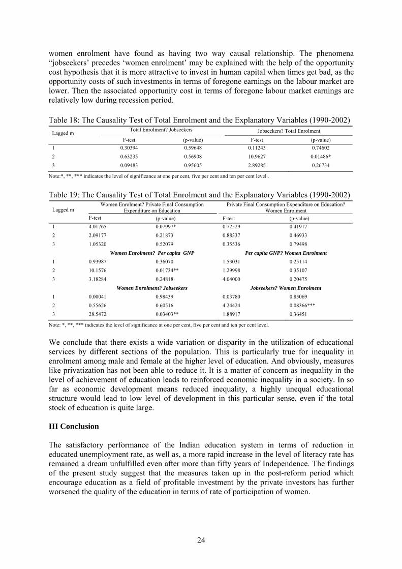
Note: *, **, *** indicates the level of significance at one per cent, five per cent and ten per cent level. During the post-reform period (Table 18 and 19), the private final consumption expenditure, as well as, per capita GNP precedes women enrolment .Which shows particularly for women enrolment at higher level factors like people’s ability to pay in terms of private final consumption expenditure on education, as well as, economic development in terms of per capita GNP precedes women enrolment .During this post-reform period jobseekers and
24
women enrolment have found as having two way causal relationship. The phenomena “jobseekers’ precedes ‘women enrolment’ may be explained with the help of the opportunity cost hypothesis that it is more attractive to invest in human capital when times get bad, as the opportunity costs of such investments in terms of foregone earnings on the labour market are lower. Then the associated opportunity cost in terms of foregone labour market earnings are relatively low during recession period. Table 18: The Causality Test of Total Enrolment and the Explanatory Variables (1990-2002)
Total Enrolment? Jobseekers Jobseekers? Total Enrolment Lagged m F-test (p-value) F-test (p-value)
1 0.30394 0.59648 0.11243 0.74602 2 0.63235 0.56908 10.9627 0.01486* 3 0.09483 0.95605 2.89285 0.26734
Note:*, **, *** indicates the level of significance at one per cent, five per cent and ten per cent level.. Table 19: The Causality Test of Total Enrolment and the Explanatory Variables (1990-2002)
Women Enrolment? Private Final Consumption Expenditure on Education
Private Final Consumption Expenditure on Education? Women Enrolment Lagged m
F-test (p-value) F-test (p-value) 1 4.01765 0.07997* 0.72529 0.41917 2 2.09177 0.21873 0.88337 0.46933 3 1.05320 0.52079 0.35536 0.79498
Women Enrolment? Per capita GNP Per capita GNP? Women Enrolment 1 0.93987 0.36070 1.53031 0.25114 2 10.1576 0.01734** 1.29998 0.35107 3 3.18284 0.24818 4.04000 0.20475
Women Enrolment? Jobseekers Jobseekers? Women Enrolment 1 0.00041 0.98439 0.03780 0.85069 2 0.55626 0.60516 4.24424 0.08366*** 3 28.5472 0.03403** 1.88917 0.36451
Note: *, **, *** indicates the level of significance at one per cent, five per cent and ten per cent level. We conclude that there exists a wide variation or disparity in the utilization of educational services by different sections of the population. This is particularly true for inequality in enrolment among male and female at the higher level of education. And obviously, measures like privatization has not been able to reduce it. It is a matter of concern as inequality in the level of achievement of education leads to reinforced economic inequality in a society. In so far as economic development means reduced inequality, a highly unequal educational structure would lead to low level of development in this particular sense, even if the total stock of education is quite large. III Conclusion The satisfactory performance of the Indian education system in terms of reduction in educated unemployment rate, as well as, a more rapid increase in the level of literacy rate has remained a dream unfulfilled even after more than fifty years of Independence. The findings of the present study suggest that the measures taken up in the post-reform period which encourage education as a field of profitable investment by the private investors has further worsened the quality of the education in terms of rate of participation of women.
25
This result has been explained with the help of the two important parameters of the estimates of returns to education. They are, ‘probability of getting job’ and ‘life-time earnings’. With the help of these two measures, we have examined the returns to education at the different levels of higher education mainly during the pre-reform period. The analysis of secondary data reveals that in the pre-reform period when the returns to higher education indicate the discounted value of ‘lifetime earnings’ less the discounted value of ‘cost’, it turned to be positive at every level of higher education, but always less for women compared to men. In the post-reform period, the logic that, the higher the rate of return the more likely that investment in education contributes is being followed. Hence, education associated with higher rates of return are those levels in which additional investment producing the greater contribution. It is this logic which explains the disparity between male and female enrolment at higher level. In a country like India, we argue, this can not be considered a desirable policy measure. Our study calls for a need for education to remain a social facility instead. Equal opportunity in education not only serves as a ‘basic need’ but also ensures that the potential intellectual talent is not lost due to wrong policy action. The effects of equal access to education are difficult to calculate (Selowsky 1973), but not unreasonable to envisage. The mal-distribution of education has both normative and economic consequences. In this study, we have explored ways to measure the relative returns and costs of education itself while striving to explain what is the result of the association between some relevant economic factors and the state of Indian higher education especially in terms of women enrolment. This is a modest beginning and much more work and careful analysis of the latest data is needed in order to formulate a more desirable approach. Endnotes
1. Among these studies only the study by Pandit (1972) is based on an all-India sample (which covered only the period 1950-1951 to 1965-1966), while others were either micro-studies or studies covering a section of population. Nallagoundan (1967), Selowsky (1967) and Blaug (1972) restricted their studies to male workers in urban India. Harberger’s (1965) study was confined to male workers in Hyderabad city while that of Chaudhri’s (1968) to male workers in rural areas of Punjab and Haryana. While the studies by Panchamukhi and Panchamukhi (1969) and Kothari (1966) were based on the city survey of Greater Bombay, the study by Chaudhri and Rao (1970) covered the graduates of Delhi University and the studies by Husain (1967) referred to Ludhiana and Lucknow. The studies by Paul (1972) and Shortlidge (1974) related to specialized branches of education at two national institutes-management education at the Indian Institute of Management, Ahmedabad, and agricultural education at the Govind Ballabh Pant University, Pantnagar, respectively.
2. Some of the earlier studies (namely, studies by Nallagoundan (1967), Selowsky (1967) and Blaug et al. (1969), Pandit (1972) and Goel (1975)) mainly used National Council of Applied Economic Research Survey data. Harberger (1957) used data on the socio-economic survey of Hyderabad city by Indian Institute of Economics. The Directorate General of Employment and Training surveys and the Ministry of Education data source have been used by Husain (1967). Duraisamy and Duraisamy (1995) used a large amount of survey data, namely, from the Degree Holders and Technical Personnel Survey, 1981. Kingdon and Unni (2001) used state-wide representative household data from two large states-Madhya Pradesh and Tamil Nadu-collected by the NSS Fourth Quinquennial Survey of Employment and Unemployment during 1987-1988 (43rd Round).

26
3. The ‘direct expenditure’ includes figure on salaries paid to the teaching and non-teaching staff, expenditure on stationary, postal expenses, telegraph and telephone charges, recurring printing charges, all recurring expenditure on laboratory, library, reading room, common room, raw materials, repair and maintenance of building, rents, rates and taxes, expenditure on games and sports, etc.
4. For almost all the studies, foregone earnings of the pupils were estimated on the basis of the age-earnings profiles, which were based on various surveys. For example, the foregone earnings derived by Tilak (1987) for his study, on the basis of the age-earnings profiles prepared from his sample survey data for Andhra Pradesh have been, for the second year (general) education, the earnings of the first year (general) graduates. Nallagoundan (1967) and Blaug (1972) in their studies simply used the data provided by the sample survey conducted by the Education Commission (1966).
References Becker, G.S. (1957), Economics of Discrimination, Chicago, University of Chicago Press. Bhagwati, J. (1973), Education, Class Structure and Income Equality, World Development, Vol. 1,
No. 5. Blaug, M. (1972), Educated Unemployment in Asia: A Contrast between India and the Phillipines,
The Philippine Economic Journal. Blaug, M., R. Layard, and M. Woodhall (1969), Causes of Graduate Unemployment in India, Allen
Lane and Penguine Press. Bloom, D. and J. Sevilla (2004), Should there be a General Subsidy for Higher Education in
Developing Countries, Journal of Higher Education in Africa, Vol. 2, No. 1. Census of India (1971a), Classification of Workers and Non-Workers by Educational level in India,
General Economic Tables in India, B-III, Part-A. ---------- (1971b), Distribution of 10,000 Non-Workers by Age-group and Type of Activity, Table B-
VIII, Part-II-B (ii). ---------- (1981a), Series 1, General Economic Tables, S-1, Part-3A (i). ---------- (1991), Percentage Distribution of Non-workers by Main Activity, Age, Sex and Residence,
India in ‘Non-Workers in India, An Analysis of the 1991 Census Data’. ---------- (1991a), Main Workers Classified by Industrial Category, Educational Level and Sex,
B-3(S). ---------- (1991b), Percentage Share of Non-workers in the Population by Age, Sex and Residence, in
‘Non-workers in India, An Analysis of the 1991 census data. ---------- (2001), Non-Workers by Main Activity, Educational Level and Sex, B-15. ---------- (2001a), Main Workers Marginal Workers, Non-workers and those Seeking/available for
Work Classified by Educational Level and Sex, B-3. ---------- (2001b), Non-workers by Main Activity, Age and Sex, B-13. Central Advisory Board of Education (CABE, 2005), Committee on Autonomy of Higher Education
Institutions, June, MHRD, Department of Secondary & Higher Education, Government of India.
Central Statistical Organisation, Statistical Abstract, Department of Statistics, Ministry of Planning, Various years.
Chaudhri, D.P. (1968), Education and Agricultural Productivity in India, Unpublished Ph. D. thesis, University of Delhi, New Delhi.
Chaudhuri, D.P. and Rao (1970), Private and Social Returns to Higher Education: a Case Study of Delhi Graduates, Economic and Political Weekly, Vol. V, No 14, 4 April.
Cohen, M.S. (1971), Sex Differential in Compensation, Journal of Human Resources (Fall). Denison, E.F. (1962), The Sources of Economic Growth in the United States and the Alternatives
Before Us, Supplementary, Paper No. 13, New York, Committee for Economic development. Duraiswamy, P. (2002), Changes in Returns to Education in India, 1983-1994, by Gender, Age
Cohort and Location, Economics of Education Review, Vol. 21, No. 6.

27
Duraiswamy, P. and M. Duraiswamy (1995), Returns to Higher Education in India, Journal of Educational Planning and Administration, Vol. IX, No.1, January.
Eckaus, R.S., A.E. Safty and V.D. Norman (1974), An Appraisal of the Calculation of Rates of Return to Higher Education, in M.S. Gordon (eds.), Higher Education and the Labour Market, New York, Mcgraw Hill.
Gadgil, D.R. (1965), Women in the Working Force in India, Asia Publishing House. Goel, S.C. (1975), Education and Economic growth in India, Macmillan, New Delhi. Gwartney, J.D. (1972), Discrimination, Achievement and Pay-offs as a College Degree, Journal of
Human Resources (Winter). Harberger, A.C. (1965), Investment in Men versus Investment in Machines: The Case in India, in
‘Education and Economic Development’, C.A. Anderson and M.J. Bowmen (Ed.), Aldine Publishing Co.
Heyneman, Stephen, P. (1979), Investment in Indian Education: Uneconomic?, World Bank Staff Working Paper, No.327, World Bank, Washington.
Husain, Ishrat Z. (1967), Returns to Education in India, in ‘Education as Investment’, Singh Baljit (Ed.), Meerat, Meenakshi Prakashan.
Kamat, A.R. (1968), Two Studies in Education, Bombay, Asia Publishing House. Kapur, D. and Mehta, P.B. (2004), Indian Higher Education Reform-from Half-baked Socialism to
Half-Backed Capitalism, Cambridge, MA: Harvard University, Center for International Development, Working Paper No.108, September.
Kingdon, Geeta Gandhi and Unni Jeemol (2001), Education and Women’s Labour Market Outcomes in India, Education Economics, Vol. 9, No. 2.
Kothari, V.N. (1966), Factor Cost of Education in India, Indian Economic Journal, Vol. 13, No. 5, April-June.
Lucas, R.E. (1988), On the Mechanics of Economic Development, Journal of Monetary Economics, Vol. 22, No. 1.
Malenbaum, Wilfred (1957), Urban Unemployment in India, Pacific Affairs XXX (March), Ministry of Human Resource Development; Education in India, Government of India, various years.
McNully, D.J. (1967), Differences in Pay between Men and Women Workers, Monthly Labor Review, December.
Nalla Gounden, A.M. (1967), Investment in Education in India, Journal of Human Resources, II Summer.
National Sample Survey Organisation (2006), Employment and Unemployment Situation in India 2004-2005, Part-I and Part-II, Ministry of Statistics and Programme Implementation, Government of India.
National Policy on Education (1986), Government of India, Department of Education, New Delhi. Panchamukhi, P.R. (1965), Devaluation of Education: A Quantitative Analysis, Journal of Higher
Education, Vol. 1, No. 1, Monsoon. Panchamukhi, P.R. and V.R. Panchamukhi (1969), Socio-economic Variables and Urban Incomes, in
H.N. Pandit (Ed.), Measurement of Cost Productivity and Efficiency of Education (1969), New Delhi, NCERT.
Pandit, H.N. (1972), Effectiveness and Financing of Investment in Education in India 1950-1951 to 1965-1966, Unpublished Ph.D. thesis, Delhi University, New Delhi.
Paul, S. (1972), An Application of Cost-Benefit Analysis to Management Education, Journal of Political Economy, Vol. 80, No. 2, March-April.
Psacharapoulos, G. (1972), Rates of Return to Investment in Education around the World, Comparative Education Review, Vol. 16.
Psacharapoulos, G. (1973), Substitution Assumptions Versus Empirical Evidence in Manpower Planning, De Economist, 121, N.R. 6.
Psacharapoulos, G. and K. Hinchliffe (1973), Returns to Education-An International Comparison, San Francisco, Jossey-Bass, Inc.
Rao, V.K.R.V. (1966), Education andHuman Resource Development, Bombay, Allied Publishers. Rao and Datta (1989), Rates of Return in the Indian Private Sector, Economics Letters, Vol. 30. Report of the University Education Commission 1948-1949 (1950), Government of India, New Delhi.
28
Selowsky, M. (1967), Education and Economic Growth: Some International Comparisons, Economic Development Report No 83, Cambridge, Harvard University (Mimeo).
---------- (1973), Investment in Education in Developing Countries: A Critical Review of Some Issues, Cambridge, Massachusetts: Center for International Affairs (Mimeographed).
Sheddy, S.C. (1983), Trends in Professional Education Among Women, Journal of Higher Education, Vol. 8, No. 3, Spring.
Shortlidge, Richard L. (1974), The Labor Market for Agricultural Graduates in India: A Benefit Cost Case Study of G. B Pant University of Agriculture and Technology, Occasional Paper No. 69, Department of Agricultural Economics, Cornell University, Ithaca, New York.
The Education Commission 1964-1966 (1971), NCERT, New Delhi. Tilak, J.B.G. (1979), Unit Cost Analysis of Higher Education in India, Journal of Higher Education,
Vol. 5, No. 2, Autumn. ---------- (1987), The Economics of Inequality in Education, Sage Publications, New Delhi. ---------- (2004), Public Subsidies in Education in India, Economic and Political Weekly, January 24. UNESCO (1977), Indian Education: A Desk Study Focused on Technical and Vocational Education,
Paris. Women’s Bureau (1969), Handbook of Women Workers 1969, U.S. Department of Labour: Women’s
Bureau Bulletin 294, US Governing Printing Office.