On the dynamics of planetesimals embedded in …piskunov/TEACHING/ASTROPHYSICS_2/nelson.pdf · On...
23
Mon. Not. R. Astron. Soc. 409, 639–661 (2010) doi:10.1111/j.1365-2966.2010.17327.x On the dynamics of planetesimals embedded in turbulent protoplanetary discs Richard P. Nelson and Oliver Gressel Astronomy Unit, Queen Mary, University of London, Mile End Road, London E1 4NS Accepted 2010 July 7. Received 2010 July 5; in original form 2010 April 29 ABSTRACT Angular momentum transport and accretion in protoplanetary discs are generally believed to be driven by magnetohydrodynamics (MHD) turbulence via the magnetorotational instability (MRI). The dynamics of solid bodies embedded in such discs (dust grains, boulders, plan- etesimals and planets) may be strongly affected by the turbulence, such that the formation pathways for planetary systems are determined in part by the strength and spatial distribution of the turbulent flow. We examine the dynamics of planetesimals, with radii between 1 m and 10 km, embedded in turbulent protoplanetary discs, using 3D MHD simulations. The planetesimals experience gas drag and stochastic gravitational forces due to the turbulent disc. We use, and compare the results from, local shearing box simulations and global models in this study. The main aims of this work are to examine: the growth, and possible saturation, of the velocity dispersion of embedded planetesimals as a function of their size and disc parameters; the rate of radial migration and diffusion of planetesimals; the conditions under which the results from shearing box and global simulations agree. We find good agreement between local and global simulations when shearing boxes of dimension 4H × 16H × 2H are used (H being the local scaleheight). The magnitude of the density fluctuations obtained is sensitive to the box size, due to the excitation and propagation of spiral density waves. This affects the stochastic forcing experienced by planetesimals. The correlation time associated with the stochastic forcing is also found to be a function of the box size and aspect ratio. The equilibrium radial velocity dispersion, σ (v r ), obtained depends on the radii, R p , of the planetesimals. Bodies with R p = 50 m achieve the smallest value with σ (v r ) 20 m s −1 . Smaller bodies are tightly coupled to the gas, and boulders with R p = 1 m attain a value of σ (v r ) similar to the turbulent velocity of the gas (∼100 m s −1 ). Equilibrium values of σ (v r ) for bodies larger than 100 m are not achieved in our simulations, but in all models we find rapid growth of the velocity dispersion for planetesimals of size 1 and 10 km, such that σ (v r ) ≥ 160 m s −1 after a run time of 1200 orbits at a distance of 5 au from the central star. These values are too large to allow for the runaway growth of planetesimals, and mutual collisions would lead to catastrophic disruption. Radial migration due to gas drag is observed for bodies with R p 1 m, and is only modestly affected by the turbulence. Larger bodies undergo a random walk in their semimajor axes, leading to radial diffusion through the disc. For our fiducial disc model, we estimate that radial diffusion across a distance of 2.5 au would occur for typical planetesimals in a swarm located at 5 au over a disc lifetime of 5 Myr. Radial diffusion of this magnitude appears to be inconsistent with Solar system constraints. Our models show that fully developed magnetohydrodynamics (MHD) turbulence in pro- toplanetary discs would have a destructive effect on embedded planetesimals. Relatively low levels of turbulence are required for traditional models of planetesimal accretion to operate, this being consistent with the existence of a dead zone in protoplanetary discs. Key words: accretion, accretion discs – MHD – methods: numerical – planets and satellites: formation – protoplanetary discs. E-mail: [email protected] (RPN); [email protected] (OG) C 2010 The Authors. Journal compilation C 2010 RAS
Transcript of On the dynamics of planetesimals embedded in …piskunov/TEACHING/ASTROPHYSICS_2/nelson.pdf · On...

Mon. Not. R. Astron. Soc. 409, 639–661 (2010) doi:10.1111/j.1365-2966.2010.17327.x
On the dynamics of planetesimals embedded in turbulentprotoplanetary discs
Richard P. Nelson� and Oliver Gressel�Astronomy Unit, Queen Mary, University of London, Mile End Road, London E1 4NS
Accepted 2010 July 7. Received 2010 July 5; in original form 2010 April 29
ABSTRACTAngular momentum transport and accretion in protoplanetary discs are generally believed tobe driven by magnetohydrodynamics (MHD) turbulence via the magnetorotational instability(MRI). The dynamics of solid bodies embedded in such discs (dust grains, boulders, plan-etesimals and planets) may be strongly affected by the turbulence, such that the formationpathways for planetary systems are determined in part by the strength and spatial distributionof the turbulent flow.
We examine the dynamics of planetesimals, with radii between 1 m and 10 km, embeddedin turbulent protoplanetary discs, using 3D MHD simulations. The planetesimals experiencegas drag and stochastic gravitational forces due to the turbulent disc. We use, and compare theresults from, local shearing box simulations and global models in this study.
The main aims of this work are to examine: the growth, and possible saturation, of thevelocity dispersion of embedded planetesimals as a function of their size and disc parameters;the rate of radial migration and diffusion of planetesimals; the conditions under which theresults from shearing box and global simulations agree.
We find good agreement between local and global simulations when shearing boxes ofdimension 4H × 16H × 2H are used (H being the local scaleheight). The magnitude of thedensity fluctuations obtained is sensitive to the box size, due to the excitation and propagationof spiral density waves. This affects the stochastic forcing experienced by planetesimals. Thecorrelation time associated with the stochastic forcing is also found to be a function of the boxsize and aspect ratio.
The equilibrium radial velocity dispersion, σ (vr), obtained depends on the radii, Rp, ofthe planetesimals. Bodies with Rp = 50 m achieve the smallest value with σ (vr) � 20 m s−1.Smaller bodies are tightly coupled to the gas, and boulders with Rp = 1 m attain a value ofσ (vr) similar to the turbulent velocity of the gas (∼100 m s−1). Equilibrium values of σ (vr) forbodies larger than 100 m are not achieved in our simulations, but in all models we find rapidgrowth of the velocity dispersion for planetesimals of size 1 and 10 km, such that σ (vr) ≥160 m s−1 after a run time of 1200 orbits at a distance of 5 au from the central star. These valuesare too large to allow for the runaway growth of planetesimals, and mutual collisions wouldlead to catastrophic disruption. Radial migration due to gas drag is observed for bodies withRp � 1 m, and is only modestly affected by the turbulence. Larger bodies undergo a randomwalk in their semimajor axes, leading to radial diffusion through the disc. For our fiducial discmodel, we estimate that radial diffusion across a distance of �2.5 au would occur for typicalplanetesimals in a swarm located at 5 au over a disc lifetime of 5 Myr. Radial diffusion of thismagnitude appears to be inconsistent with Solar system constraints.
Our models show that fully developed magnetohydrodynamics (MHD) turbulence in pro-toplanetary discs would have a destructive effect on embedded planetesimals. Relatively lowlevels of turbulence are required for traditional models of planetesimal accretion to operate,this being consistent with the existence of a dead zone in protoplanetary discs.
Key words: accretion, accretion discs – MHD – methods: numerical – planets and satellites:formation – protoplanetary discs.
�E-mail: [email protected] (RPN); [email protected] (OG)
C© 2010 The Authors. Journal compilation C© 2010 RAS

640 R. P. Nelson and O. Gressel
1 IN T RO D U C T I O N
The dynamical and collisional evolution of planetesimals is a fun-damental issue which needs to be understood if progress is to bemade in developing a theory of planetary system formation. Accord-ing to the core accretion theory, a process which begins with thecollision and sticking of small dust grains within a protoplanetarydisc leads eventually to the formation of kilometre-sized planetes-imals (Wetherill & Stewart 1993). Although alternative scenarioshave been put forward for planetesimal formation (Goldreich &Ward 1973; Johansen et al. 2007), which avoid the requirement forsuch large bodies to grow via simple two-body agglomeration pro-cesses, the further growth of planetesimals into planetary embryosand cores generally requires planetesimals themselves to accrete viamutual collisions through a process of runaway growth, followedby oligarchic growth (Ida & Makino 1993; Kokubo & Ida 1998).
Rapid runaway growth requires that the velocity dispersion of theplanetesimal swarm remains significantly smaller than the escapevelocity from the surfaces of the largest accreting planetesimals,ensuring that gravitational focusing is important. For bodies of ra-dius 10 km, and with internal densities �p � 2 g cm−3, the escapevelocity is 10 m s−1, and scales linearly with radius. Clearly this isa stringent requirement, which is easily met within a self-stirringplanetesimal swarm whose size distribution is reasonably shallow,but which may be difficult to satisfy in the presence of an externalsource of stirring. One such source may be turbulence within theprotoplanetary disc. Planetary growth times which rely on mutualcollisions between planetesimals occurring at rates which are deter-mined by the geometric cross-section are prohibitively long, leadingto estimated planetary growth times which are much in excess oftypical protostellar disc lifetimes (Haisch, Lada & Lada 2001).
A further constraint during the runaway growth phase is thatcollisional velocities should be small enough to avoid catastrophicdisruption of planetesimals. For bodies in the 1–10 km size range,for which self-gravity starts to become more important than mate-rial strength in holding planetesimals together, collisions betweensimilar-sized bodies with impact speeds which are modestly in ex-cess of the escape velocity will lead to breakup of the planetesimalsrather than accretion and growth. Indeed Benz & Asphaug (1999)suggest that mutual collisions between 1 km sized bodies will resultin catastrophic disruption if the impact speeds exceed ∼20 m s−1,depending on the material composition of the impactors. In a morerecent study, Stewart & Leinhardt (2009) suggest reduced impactspeeds of ∼10 m s−1 will be destructive. Once again, we see thatan external source of planetesimal stirring may prevent the rapidgrowth of planetary mass bodies by the accretion of planetesimals.
The canonical mass accretion rate for T Tauri stars is∼10−8 M� yr−1 (Sicilia-Aguilar et al. 2004). Such accretion ratesrequire a source of anomalous disc viscosity and angular momen-tum transport to operate, generally thought to be turbulence. Themost likely source of disc turbulence is the magnetorotational in-stability (MRI; Balbus & Hawley 1991) which has been shown todevelop into full non-linear magnetohydrodynamics (MHD) turbu-lence in numerous studies, using both local shearing box simulations(Hawley, Gammie & Balbus 1995) and global simulations(Armitage 1998; Hawley 2001; Papaloizou & Nelson 2003). Thenature and saturation state of MHD turbulence generated by theMRI is the subject of on-going study (Fromang & Papaloizou 2007;Fromang et al. 2007). In this work, we use the dependence of theturbulent stresses and density fluctuation amplitude on the strengthof the net component of the magnetic field to examine the evolutionof planetesimals in discs with different levels of turbulence. We
use simple disc models, which neglect non-ideal MHD effects andvertical stratification. As such, this is the first in a series of papersin which we examine how turbulence affects the dynamics of plan-etesimals embedded in turbulent discs. Future papers will explorethe effects of vertical stratification and dead zones.
There have been numerous studies of planets embedded in turbu-lent protoplanetary discs. Nelson & Papaloizou (2003) and Winters,Balbus & Hawley (2003) examined the formation of gaps by Jovianmass planets, and the migration torques exerted by the disc on theplanet. Nelson & Papaloizou (2004) performed global simulationsof low-mass planets embedded in turbulent discs. They showedthat such bodies are subject to fluctuating torques which shouldinduce stochastic migration, and suggested that this might providea means of mitigating against the rapid type I migration expectedto occur for low-mass planets (Ward 1997). Laughlin, Steinacker& Adams (2004) published a similar study using analytical fits toMHD simulations, and reached similar conclusions. Papaloizou,Nelson & Snellgrove (2004) presented results from both global andlocal shearing box simulations containing both high- and low-massplanets, and showed good agreement between the simulation set-ups for predicting the transition between linear and non-linear discresponse to the presence of an embedded planet. In a follow-uppaper, Nelson (2005) examined the orbital evolution of low-massembedded planets, showing that over simulations run times of �100orbits, turbulence induces stochastic migration for planets in therange 1–10 M⊕, and induces the growth of orbital eccentricity. In amore recent work, Oishi, Mac Low & Menou (2007) examined thestochastic forces experienced by planets in stratified disc modelswith and without dead zones using shearing box simulations, andYang, Mac Low & Menou (2009) examined the orbital evolution ofswarms of test particles embedded in non-stratified turbulent discs.
A significant volume of related work has examined the influ-ence of disc turbulence on embedded planets and planetesimalsusing prescriptions or simple models for the effects of turbulence.Johnson, Goodman & Menou (2006) developed a Fokker–Planckdescription for the stochastic evolution of planets, and examinedthe survival probabilities of distributions of planets subject to typeI migration and superposed stochastic migration. A similar studyhas been published recently by Adams & Bloch (2009). Ogihara,Ida & Morbidelli (2007) have used N-body simulations plus a pre-scription for stochastic forcing to examine the effects of turbulenceon terrestrial planet formation. Ida, Guillot & Morbidelli (2008)used a similar prescription of turbulent forcing and examined thegrowth of eccentricity for planetesimals, exploring in particular thepossibility of reaching catastrophic disruption velocities. Adams,Laughlin & Bloch (2008) and Rein & Papaloizou (2009) examinedthe stability of mean motion resonances for pairs of planets embed-ded in turbulent discs, and Baruteau & Lin (2010) have examinedthe saturation of corotation torques in turbulent discs by means ofhydrodynamic simulations subject to turbulent stirring.
In this paper, we examine in detail the orbital evolution of plan-etesimals of different size (ranging between 1 m and 10 km) em-bedded in turbulent disc models by means of 3D MHD simulations.A key issue that we explore is the set of conditions and numericalparameters that provide good agreement between local shearing boxsimulations and global simulations. We find that it is possible to ob-tain good agreement between these two numerical set-ups, providedthat the shearing box dimensions are chosen appropriately. Otherimportant issues that we examine include the growth of the velocitydispersion of embedded swarm of planetesimals, and the saturationvalue of this velocity dispersion as a function of planetesimal sizedue to a balance being achieved between gas drag and turbulent
C© 2010 The Authors. Journal compilation C© 2010 RAS, MNRAS 409, 639–661

Dynamics of planetesimals in turbulent discs 641
forcing. We explore the implications of our results for the efficiencyof runaway growth of planetary embryos, and the possibility thatplanetesimals may enter a phase of catastrophic disruption throughmutual collisions. We also examine the rate at which planetesimalsmigrate due to both gas drag induced radial drift (Weidenschilling1977), and diffusion caused by the fluctuating gravitational fieldof the turbulent disc. We examine under which conditions each ofthese processes is dominant, and we explore the implications of ourresults for the radial drift of planetesimals in the solar nebula andlimits that might be placed on the magnitude of turbulent fluctua-tions which were present during the early phases of Solar systemformation.
This paper is organized as follows. In Section 2, we describethe numerical set-up and the parameters of the disc models. InSection 3 we present our results. In Section 4 we discuss our workin the context of previous work and draw our conclusions.
2 MODEL DESCRIPTION
We perform self-consistent simulations of hydromagnetic turbu-lence using two different set-ups: shearing box simulations whichrepresent a local patch of a protoplanetary disc; global disc modelswhich simulate a larger section of a protoplanetary disc and includethe full set of curvature terms in the equations of motion. A majorgoal of this work is to compare the results of these two differentapproaches.
A key question that needs to be addressed is for what dimensionsof the shearing box, in units of the local scaleheight H, do densityfluctuations created by the turbulence reach a converged amplitudeand spectrum, and do these match the results of global models. Tomake the comparison as straightforward as possible, we neglectvertical stratification and assume an isothermal equation of state.
In both configurations, the hydromagnetic turbulence is drivenvia the non-linear development of the MRI. At present, the issue ofthe saturated amplitude of MRI turbulence remains unresolved andis a topic of active research (Fromang & Papaloizou 2007; Fromanget al. 2007). In the absence of a better alternative, we thereforeadopt a practical perspective and impose a net vertical or azimuthalflux, for which numerical convergence can be obtained (Davis,Stone & Pessah 2010). Neglecting the dependence on the magneticPrandtl number (Lesur & Longaretti 2007), we furthermore restrictourselves to the case of ideal MHD. This approach is justified bythe observed correlation between the strength of the turbulenceand the amplitude of the resulting density fluctuations (Yang et al.2009). This means that we regard the strength of the imposed fieldas a control parameter which can be tuned to vary the turbulenceamplitude in the local and global context. The global cylindricaldisc models are computed with a modified version of the originalfinite difference code NIRVANA (Ziegler & Yorke 1997). For the localshearing box models, we make use of the newly developed second-order Godunov code NIRVANA-III (Ziegler 2004, 2008).
2.1 Numerical methods – local model
For our standard model, we adopt a box size1 of 4 × 16 × 2 pressurescaleheights H at a resolution of 32 grid points per H. Boundaryconditions are periodic in the azimuthal (y) and vertical (z), andsheared-periodic in the radial (x) direction. The initial net verticalmagnetic field corresponds to a plasma parameter β � 6000 (i.e.
1 See Section 3.3 for a discussion on the effect of the box size.
the ratio of thermal to magnetic pressure), resulting in a typicalsaturation level α � 0.05 of the turbulence, where α is the effectiveviscosity parameter (Shakura & Syunyaev 1973).
Because the gas drag forces acting on massive particles dependon the actual physical value of the gas density, we have to prescribea set of conversion factors to link our model to a representativeprotoplanetary disc. We chose a fiducial radius R0 = 5 au, and ageometric disc thickness of H/R = 0.05 at R = 1 au. Note that thisaspect ratio is scaled with R1/4 to be consistent with the Hayashiminimum mass solar nebula (MMSN; Hayashi 1981), yielding avalue of �0.075 at 5 au. Furthermore, we chose a slightly higheraverage mass density than in this model to yield a column density� = 160 g cm−2 and sound speed cs = 1 km s−1 comparable to theglobal simulations.
For the local model, we evolve the following set of non-linearpartial differential equations:
∂t � +∇ · (�v) = 0,
∂t (�v) +∇ ·[�vv +
(p + B2
2μ
)I − BB
μ
]=−2�� z× (v + q�x y)
∂tB − ∇ × (v × B) = 0, (1)
comprising the standard formulation of ideal MHD in the shearingbox approximation, and where we have assumed an isothermalequation of state p = �c2
s and neglected the effects of stratification.The two momentum source terms are the Coriolis force −2�z×v inthe locally corotating frame, and the tidal term 2q�2x x, with shear-parameter q = 3/2, describing the linearized effect of the Keplerianrotation.2 Care has been taken in implementing the source terms tominimize the error in the epicyclic mode energy (Gressel & Ziegler2007), albeit not to the extent where it is conserved to machineaccuracy (Stone & Gardiner 2010).
2.1.1 Numerical scheme and orbital advection
As has been recently demonstrated by Balsara & Meyer (2010), theadequate modelling of the MRI with finite volume codes dependson the reconstruction strategy used and, in particular, on the abil-ity of the Riemann solver to capture the Alfven mode. To improvethe treatment of discontinuities in the Godunov scheme, we there-fore extended NIRVANA-III with the Harten–Lax–van Leer Discontinu-ities (HLLD) approximate Riemann solver proposed by Miyoshi &Kusano (2005).
In accordance with its finite volume approach, the NIRVANA-III
code evaluates the components of the electromotive force (EMF) atcell interfaces. Since the discretization of the constrained transportalgorithm intrinsically requires edge-aligned EMFs, some sort of in-terpolation is required. In its original form, NIRVANA-III implementsthe arithmetic average proposed by Balsara & Spicer (1999). Asdiscussed in section 3.2 of Gardiner & Stone (2005), this approachhowever lacks the required directional biasing to guarantee the sta-bility of the numerical scheme. It has further been demonstrated byFlock et al. (2010) that this can lead to artificial growth of instabil-ities in the context of net-flux MRI, and we have reproduced thisresult. To resolve this issue, we have successfully implemented andtested the upwind reconstruction procedure of Gardiner & Stone(2005).
Following the long-term evolution of a shearing flow in boxesof substantial radial extent puts high demands on computational
2 The variable x = R − R0 is the radial displacement from the box centre.
C© 2010 The Authors. Journal compilation C© 2010 RAS, MNRAS 409, 639–661
642 R. P. Nelson and O. Gressel
resources. For a Keplerian rotation profile, the background flowbecomes super-sonic for Lx > 4/3H. This implies that for increas-ingly larger boxes the numerical time-step, defined by the Courantcondition, becomes dominated by the unperturbed shear profile. Tocircumvent this undesirable constraint, it becomes mandatory tosplit-off the transport term due to the background profile.
The shear transport is usually implemented in terms of an inter-polation step. This was first introduced in cylindrical geometry andtermed FARGO by Masset (2000). Later, the method was adoptedto the local shearing box model by Gammie (2001).
A rather intricate extension for the induction equation that re-quires mapping of the magnetic field components has been pro-posed by Johnson, Guan & Gammie (2008). We here follow the(much simpler) constrained transport approach proposed by Stone& Gardiner (2010), which by construction preserves the solenoidalconstraint.
For our implementation of the orbital advection scheme, weoperator-split the advection step from the Runge–Kutta time in-tegration of the remaining terms. For the interpolation of the fluidvariables, we make use of the high-order Fourier scheme [shearadvection by Fourier interpolation (SAFI)] described in appendixB of Johansen, Youdin & Klahr (2009).
We similarly apply SAFI to obtain the non-integer part of theline-integrals which contribute the circulation of the electric fieldsentering the induction equation (cf. equations 61 and 62 in Stone &Gardiner 2010). The treatment of the magnetic source term in thetotal energy equation can be successfully avoided if the magneticenergy is removed from the total energy during the interpolation.The implementation has been tested with the advection of a fieldloop (Gardiner & Stone 2008), and the exact wave solution givenin Balbus & Hawley (2006).
Using SAFI rather than slope-limited linear interpolation, effi-ciently reduces the dissipation due to the transport step, and more-over its dependence on position (see Johansen et al. 2009). In fact,the scheme adds so little dissipation that the total variation dimin-ishing (TVD) requirement might be violated. To formally make theinterpolation TVD, we therefore discard the Fourier mode corre-sponding to the Nyquist frequency.
2.1.2 Particle dynamics
In this paper, we restrict ourselves to the study of how disc turbu-lence affects embedded particle populations. Neglecting their backreaction on the flow, particles are hence treated as passive test bod-ies which do not interact mutually either through physical collisionsor through gravity. Under these assumptions, we ignore the possi-bility of increasing the velocity dispersion of particles via mutualgravitational scattering. While this effect might become importantfor ∼102 km-sized objects, it simply adds to the external stirring.Physical collisions between planetesimals, however, can provide asource of damping. This effect was considered by Ida et al. (2008),and was found to be important in determining the equilibrium ve-locity dispersion only for bodies with size <1 km, and so we do notconsider this effect in this paper. Moreover, because the particlescannot exert drag forces on the gas, our approach excludes collectiveeffects such as the streaming instability (Youdin & Goodman 2005),which is a focus of current numerical studies (Youdin & Johansen2007; Balsara et al. 2009; Bai & Stone 2010; Miniati 2010).
We include different species of particles to quantify various as-pects of the flow. First, massless tracer particles (which instanta-neously follow the gas velocity) measure the Lagrangian diffusion
of the flow. This is relevant for small dust grains which are tightlycoupled to the gas. Secondly, we include particles representing plan-etesimals. These particles interact with the flow via the gravitationalpotential produced by the gas density, and through the aerodynamicdrag force. The relative importance of these effects is expected tochange for planetesimals in the size range 1 m to 10 km, which arethe subject of this study. Finally, for the purpose of comparison, andas a proxy for larger objects (e.g. small protoplanets), we includeswarms of particles which experience gas gravity but are not subjectto an aerodynamic drag force. With the exception of the tracers, allparticles are subject to the local dynamics, i.e. they experience theCoriolis force in the rotating frame and the tidal force stemmingfrom the local expansion of the Keplerian rotation profile. As a con-sequence, planetesimals generally perform epicyclic oscillations offluctuating amplitude, around a stochastically migrating guidingcentre.
2.2 Numerical method – global model
In the global simulations, we solve essentially the same set of equa-tions for ideal MHD as described in Section 2.1 for the shearingbox runs, except that we adopt cylindrical coordinates (r, φ, z) (seeNelson 2005 for a full description). The simulations are performedin a rotating frame with angular frequency equal to the Keplerianfrequency at the midpoint of the radial computational domain. Weuse a locally isothermal equation of state
P (r) = cs(r)2 �, (2)
where cs(r) denotes the sound speed which is specified as a fixedfunction of r. The models investigated may be described as cylin-drical discs (e.g. Hawley 2001), in which the gravitational potentialis taken to depend on r alone. Thus, the cylindrical disc models donot include a full treatment of the disc vertical structure. Models ofthis type are employed due to the high computational overhead thatwould be required to fully resolve the disc vertical structure of astratified model.
The global simulations presented in this paper were performedusing an older version of NIRVANA, which uses an algorithm verysimilar to the ZEUS code to solve the equations of ideal MHD (Stone& Norman 1992; Ziegler & Yorke 1997). This scheme uses operatorsplitting, dividing the governing equations into source terms andtransport terms. Advection is performed using the second-ordermonotonic transport scheme (van Leer 1977), and the magneticfield is evolved using the Method of Characteristics ConstrainedTransport (Hawley & Stone 1995).
2.2.1 Gas disc model
The main aim of this paper is to examine the orbital evolutionof planetesimals and smaller bodies (boulders) in turbulent discs,where the disc turbulence has achieved a well-defined steady state.Another aim is to compare local shearing box runs with globalsimulations. To achieve these aims, most of the global disc modelswere chosen to have a relatively narrow radial extent, and azimuthaldomains running between 0 ≤ φ ≤ π/2. The turbulent stressesgenerated within a global disc lead to significant changes in theradial density distribution, such that the properties of the disc deviatesubstantially from a statistical steady state over runs times of 100 sof orbits (Papaloizou & Nelson 2003). In order to overcome this,we have introduced an additional equation to be solved alongsideequations (1) in the global simulations, whose purpose is to maintain
C© 2010 The Authors. Journal compilation C© 2010 RAS, MNRAS 409, 639–661

Dynamics of planetesimals in turbulent discs 643
a roughly constant surface density profile during the runs:
d�(t)
dt= −�(t) − �0
τm. (3)
Here �(t) is the density at each spatial location in the disc at time t,�0 is the initial density defined at each location in the disc and τm isthe characteristic time on which the local perturbed density evolvesback towards its original value. Clearly, if τm is shorter than anyrelevant local dynamical time in the disc, then perturbations willbe damped very quickly and the disc will not be able to achievea turbulent state. Similarly, if τm is much longer than the longest(viscous) evolution time in the disc, the global density profile will beable to evolve to be very different from the initial one. By choosingτm to be intermediate between these two extremes, we find thatour global disc models are able to develop a well-defined turbulentstate, in which the turbulence is able to maintain an approximatestatistical steady state over long time-scales (>103 orbits). We havefound that τm = 50 orbits measured at the radial midpoint of thedisc model provides a model with the desired properties.
A possible alternative to solving equation (3) would be to feedin mass at the outer radial boundary at the requisite rate. Such anapproach works well as a means of generating a steady disc whenthe disc is laminar and employs the α-model for viscosity (Masset2002). In a turbulent disc, where there is substantial temporal andspatial variation in the viscous stress, however, such an approachmay not be effective at maintaining a well-defined surface densityprofile.
2.2.2 Initial and boundary conditions
Each global model has a value for the inner and outer radii of thecomputational domain, rin and rout, a value for the height of theupper and lower ‘surfaces’ of the disc, Zmin and Zmax, and minimumand maximum values of the azimuthal angle, φmin and φmax. Thesevalues are tabulated in Table 1, along with some of the physicalparameters described below. The resolution used in each simulationcovering π/2 in azimuth was (Nr, Nφ , Nz) = (160, 320, 40). For themodel covering 2π in azimuth Nφ = 1280. This corresponds to 10cells per mean scaleheight in the radial and azimuthal directions, and20 cells per scaleheight in the vertical domain. When consideringthe behaviour of the correlation time for the fluctuating torques inSection 3.3.1, we also ran models with double and quadruple theresolution in the radial and azimuthal directions.
The unit of length in our simulations is taken to be 2 au, suchthat a radial distance of r = 2.5 in computational units correspondsto 5 au. The unit of mass is assumed to be the solar mass. Whenwe discuss the temporal evolution of our models later in the paper,we adopt a time unit which is equal to the orbital period at r = 2.5(equivalent to 5 au); this being the midpoint of our radial domain.
The disc models we adopt are similar locally to the MMSN model(Hayashi 1981) at a distance of 5 au from the star. All models havea constant aspect ratio H/r, and all but one model has H/r = 0.05.
Model G5 has H/r = 0.075 for the purpose of comparing directlywith the local shearing box models (where this value of H/r wasused). Initially, the density is constant, such that the surface density� = 150 g cm−3.
The initial magnetic field in the global runs is purely toroidal,with the local field strength being determined from the local plasmaβ parameter (β = Pgas/Pmag). The value of β used in each run istabulated in Table 1. The field is introduced at all locations in thedisc, except near the radial boundaries where the field is set to zerofor r − rin < 0.1 and rout − r < 0.1. The initial disc velocity isdetermined according to
vφ = r
√√√√GM∗r3
[1 −
(H
r
)2], (4)
where M� is the mass of the central star, with the other velocitycomponents being set to zero. Prior to a run being initiated, however,all velocity components are seeded with random noise with anamplitude equal to 5 per cent of the local sound speed.
Each disc model described in Table 1 was evolved until the tur-bulence reached a quasi-steady state before the planetesimals wereinserted. Most runs included planetesimals of size 10 m, 100 m,1 km and 10 km, with each size being represented by 25 particles.The planetesimals were distributed randomly in a narrow annuluscentred on the computational radius r = 2.5 (equivalent to 5 auin physical units) of width �r = 0.2, with their initial velocitiescalculated such that they are on circular orbits under the influenceof the instantaneous gravitational potential of the central star andturbulent disc.
We adopt periodic boundary conditions at the vertical and az-imuthal boundaries, and reflecting boundary conditions at the ra-dial boundaries. Furthermore, we use wave damping boundary con-ditions in the vicinity of the radial boundaries using the schemedescribed in de Val-Borro et al. (2006). This scheme relaxes thevelocity and density near the boundaries towards their initial valueson a time-scale equal to 10 per cent of the local orbital period.
2.3 Gravitational forces
Both the local and the global models calculate the gravitational po-tential of the gas at the position of the particles via direct summation.This is computationally favourable as long as one is only interestedin a relatively small number of particles. Since we do not considercollective effects, an ensemble of a few tens of members is usuallysufficient to reasonably determine the time-averaged distribution oftheir positions and velocities.
For the integration of the gravitational force, the mass containedwithin a grid cell is treated as a point source located at the cell centre.To avoid artefacts due to close encounters, we apply a commonsmoothing length formalism with a parameter b = (δ2
x + δ2y)
1/2
equal to the diagonal across the cell.
Table 1. Global simulation parameters and results.
Simulation rin/rout φmax Zmin/Zmax H/r β 〈α〉 〈δ�/�〉 〈δ�/�〉 Cσ (vr)/(cs × 10−3) Cσ (�a)/(10−4)
G0/G1 1.5/3.5 π/2 ±0.125 0.05 50 0.035 0.143 0.109 8.87 ± 0.50 7.92 ± 0.69G2 1.5/3.5 2π ±0.125 0.05 50 0.040 0.159 0.124 8.20 ± 0.32 12.20 ± 0.56G3 1.5/3.5 π/2 ±0.125 0.05 200 0.017 0.101 0.088 8.18 ± 0.41 7.17 ± 0.39G4 1.5/3.5 π/2 ±0.125 0.05 12.5 0.105 0.266 0.150 11.30 ± 0.70 10.00 ± 0.10G5 1.0/4.0 π/2 ±0.187 0.075 50 0.034 0.126 0.094 4.69 ± 0.21 7.65 ± 0.67
C© 2010 The Authors. Journal compilation C© 2010 RAS, MNRAS 409, 639–661

644 R. P. Nelson and O. Gressel
Figure 1. Convergence study regarding the computation of the gravitationalforce via direct summation; the convergence order is approximately 3/2.
As can be seen in fig. 2 of Heinemann & Papaloizou (2009b), theturbulence driven by long-wavelength MRI modes leads to the for-mation of strong density waves, which develop very little structurealong the vertical direction. Accordingly, we neglect the verticalcomponent of the forces and adopt a cylindrical description wherethe gravity now only depends on the vertically integrated columndensity. This approach greatly reduces the computational demandand is consistent with neglecting the vertical density stratification.As we will see in Section 3.3, this 2D treatment enhances the gravityforces by a factor of roughly 2.
When considering local shearing box simulations in particular,a question that needs to be answered is how large a shearing boxis required before the gravitational forces from a turbulent disc areconverged. In Fig. 1, we plot the relative error of the gravity forcewhen integrating over spheres with increasing radius. We see that,for values accurate at the per cent level, one requires a sphere ofinfluence with a radius of about 10 pressure scaleheights. As ex-pected, forces in the azimuthal direction are affected more stronglyby long-range contributions. Because the net effect is determined bydensity fluctuations, the convergence is weaker than the r−2 depen-dence for the Newtonian gravity. We consequently find a smallerconvergence order of about 3/2. In our local simulations, we adopta sphere (cylinder) with rcl = 16H, within which we compute thegravitational acceleration on a planetesimal, and suitably extendthe domain by mirroring ghost domains according to the shearedperiodicity.
In the global simulations the gravitational field is computed bysumming over all grid cells. Most simulations were run using anazimuthal domain of π/2, although the planetesimal orbits cover thefull 2π domain. When calculating the gravitational field experiencedby the planetesimals, additional copies of the disc, each shifted bynπ/2, where n ∈ {1, 2, 3}, are used to mimic a disc which coversthe full 2π in azimuth. One run with a full 2π azimuthal domainwas run to check that the above procedure gives accurate results.
2.4 Gas drag
For the gas drag, we use the usual formulae for the Stokes and Ep-stein regimes (Weidenschilling 1977; Rafikov 2004). In the Epsteinregime, the drag force is given by
Fdrag = (vg − vp) τ−1s , (5)
with the stopping time
τs = �pRp
�cs, (6)
where Rp is the physical radius of the planetesimal, � is the gasdensity at the position of the planetesimal, �p is the internal densityof the planetesimal, vp is the planetesimal velocity and vg is the gasvelocity. In the Stokes regime it may be written
Fdrag = 1
2CDπR2
p� |vp − vg| (vp − vg), (7)
where CD is the drag coefficient, which takes the values
CD =⎧⎨⎩
24. R−1e Re < 1
24. R−0.6e 1 < Re ≤ 800
0.44 Re > 800,
(8)
where Re is the Reynolds number of the flow around the planetesi-mals, defined by
Re = 2Rpvpg/νp, (9)
where vpg = |vp − vg|, and the molecular viscosity of the flowaround the planetesimal is given by
νp = λcs/3 (10)
in most of the global simulations we have performed. It should benoted that in the local simulations, however, the molecular viscositywas defined by
νp = λcs/2, (11)
so we have run one global model (G5) adopting this value. Themolecular mean-free path λ = (nσH2 )−1, where n = �/(μmH) is thenumber density of particles, μ is the mean molecular weight, andmH is the mass of the hydrogen atom. All but one global simulationadopted the assumption that the disc gas is composed entirely ofmolecular hydrogen, giving μ = 2. The local shearing box modelsadopted a value of μ = 2.4, so we have run one global model (G5)using this value in order to provide a direct comparison betweenlocal and global models. We adopt a value of σH2 = 10−15 cm2 forthe collision cross-section of molecular hydrogen (Rafikov 2004).Trilinear interpolation is used to obtain the gas density and velocityat the position of each planetesimal.
The time integration of the particle motion in the shearing boxsimulations was performed as follows. Because the gas drag rela-tions are of the form vα in the relative velocity v = |vg − vp|, theupdate can be performed analytically. In the case α = 1, the relevanttime-scale ω−1 is just the classical stopping time, and the decay isexponential. The update from time tn to time tn+1 with time-step δtcan then be written as
vn+1 = vn e−ω δt . (12)
For α �= 1, we obtain power-law solutions for the damping of therelative velocity, which can be expressed as
vn+1 = [v1−α
n (1 + (α − 1) ω δt)] 1
1−α , (13)
where ω−1 is now a generalized ‘stopping time’ defined by ω =fdr v
−1, with f dr the specific drag force acting on the particle.In the global simulations, the particles were evolved using a fifth-
order Runge–Kutta scheme (Press et al. 1996).
3 R ESULTS
We organize the discussion of our results by first describing theevolution of the disc models. We then describe the evolution ofthe velocity dispersion (or equivalently eccentricity) of embeddedplanetesimals, followed by a discussion of their migration throughchanges in the semimajor axes.
C© 2010 The Authors. Journal compilation C© 2010 RAS, MNRAS 409, 639–661

Dynamics of planetesimals in turbulent discs 645
3.1 Hydromagnetic turbulence – local model
Restricting one’s consideration to a local approach, one mightnaıvely think that a relatively small box should suffice to capturethe relevant dynamics (see Regev & Umurhan 2008, for a generaldiscussion on limitations of the local approximation). As can beseen in Fig. 2, this notion is supported by looking at the turbulentstresses created by the saturated MHD turbulence. Taken as theonly criterion, one arrives at the conclusion that box sizes of � 4H
are sufficient to study the local stirring of particles – but this ismisleading as the gravitational torques acting on the planetesimalsare strongly affected by spiral density waves, which arise as a sec-ondary feature of the vigorously driven turbulence in a shearingbackground.
In a series of two papers, Heinemann & Papaloizou (2009a,b)study the mechanisms by which spiral density waves are excitedin a differentially rotating fluid. One important conclusion of theirwork is that a minimum azimuthal extent Ly � 6H is requiredto properly capture the dynamics of spiral waves. This is exactlywhat we see when looking at the autocorrelation function (ACF) ofthe vertically integrated density, as plotted in Fig. 3. Here the thickblack line indicates the contour where the correlation falls off to e−1,and we see that density structures are predominantly trailing waveswith an azimuthal extent of about six pressure scaleheights. Theaspect ratio of the approximate ellipse is about one-sixth, indicatingthat convergence in the radial direction should be obtained muchearlier (cf. right-hand panel of Fig. 8).
Returning to Fig. 2, we see that this requirement is reflectedin the relative rms density fluctuations 〈δ�/�〉 measured in the
Figure 2. Box size-dependence of key indicators characterizing the hydro-magnetic turbulence: while both the Reynolds and Maxwell contributionsto the turbulent stress are well converged for azimuthal box sizes aboveLy � 4H , the effected density waves are clearly suppressed in too smallboxes. Converged values for the relative density fluctuation can only beobtained for Ly � 8H . This is directly reflected in the gravitational torquesacting on the particles (cf. Fig. 8).
Figure 3. 2D ACF of the vertically integrated gas density, computed fromsix uncorrelated snapshots of a simulation with box size 4H × 16H × 2H.The thick black contour indicates a value of e−1 while the thick grey linemarks the first zero-crossing.
saturated turbulent state (uppermost curve in Fig. 2). Increasingthe box size from 2H to 8H results in an increase of ∼75 percent in the relative rms fluctuations. This is considerably largerthan the ∼25 per cent increase found by Yang et al. (2009), whoperformed a similar study. As the authors themselves mention, eventhis not particularly dramatic effect seems to strongly affect particlestirring. This can be understood when taking into account the centralfinding of the simulations undertaken in Heinemann & Papaloizou(2009b), namely that spiral density waves quickly grow into thenon-linear regime where they develop steep shock-like features. Itseems natural that the resulting intermittent density structure createshighly fluctuating torques, gravitationally enhancing the turbulentvelocity dispersion of embedded planetesimals. We examine thisissue in more detail in Section 3.3.
3.2 Hydromagnetic turbulence – global models
Prior to inserting the planetesimals in the global disc models, weallow the MRI to develop into quasi-steady non-linear MHD tur-bulence, with well-defined volume-averaged stresses operating. Anexample of the time history of the Maxwell, Reynolds and totalvolume-averaged stress (taken from model G0/G1) is presented inFig. 4, and the total stress generated in each of the models as afunction of time is shown in Fig. 5. It is clear that the models have
Figure 4. Contributions of the Reynolds (lower) and Maxwell (middle line)stresses to the effective α parameter (upper line) versus time for model G1.
Figure 5. Evolution for the total α value for the models G1, G3, G4 and G5described in Table 1.
C© 2010 The Authors. Journal compilation C© 2010 RAS, MNRAS 409, 639–661

646 R. P. Nelson and O. Gressel
evolved to a quasi-steady state. The turbulence generates a distri-bution of density and surface density fluctuations which are wellfitted by Gaussian distributions. The computed standard deviationsfor these Gaussian fits (which we denote as 〈δ�/�〉 and 〈δ�/�〉)are tabulated in Table 1 for each disc model, along with the time-averaged stress parameter α. As can be seen from Table 1, ourmodels generate α values in the range 0.017 ≤ α ≤ 0.101, withcorresponding rms values for 〈δ�/�〉 in the range 0.101 ≤ 〈δ�/�〉≤ 0.266.
In terms of physical parameters, the global model which is mostsimilar to the shearing box simulation is run G5. We see that α �0.05 in Fig. 2 for the shearing box simulation, whereas α = 0.035for model G5 because of the differing magnetic field topologies andstrengths. The density fluctuations for the shearing box model give〈δ�/�〉 = 0.17, whereas 〈δ�/�〉 = 0.13 for model G5.
In Section 3.1, it was shown that the two-point correlation func-tion for the density field obtained in local shearing box simulationswas highly anisotropic, with structure in the azimuthal directionbeing stretched by a factor of ∼6 relative to the radial direction. Weplot the corresponding two-point correlation function for model G1in Fig. 6. It is very similar to that shown in Fig. 3 for the shear-ing box run, indicating strong similarities in the density structuresobtained in local and global simulations.
3.3 Gravitational torques versus shearing box size
To illustrate the strong dependence of the disc gravity on the domainsize in local simulations, we performed sets of runs with varyingradial and azimuthal extents of the box. As a measure of the mag-nitude of the stirring, we record time series of gravitational torquesat fixed positions and compute the width of the resulting distribu-tion function. This is exemplified in Fig. 7, where we see that, onlyfor large-enough boxes, the torques are consistent with a normal
Figure 6. Contours of the two-point correlation of the surface density av-eraged over six snapshot from model G1. The heavy contours represent thee−1, and the zero level is represented by the grey line.
Figure 7. Time-averaged distribution of the gravitational torques acting ona set of particles. Left: small box, the distribution shows excess of bothlarge and small values (as typical for intermittency). Right: large box, thehistogram is well represented by a normal distribution centred around zeroand with a standard deviation of 1.48 × 108 cm2 s−2.
Figure 8. Left: specific gravitational torques versus box size as determinedby fitting a normal distribution (cf. Fig. 7). Gravitational torques computedvia the column density (‘2D force’) are consistently enhanced by a factor ofroughly 2, as expected from a simple geometric argument. Right: isolationof the effects due to variation in Lx, and Ly, respectively.
distribution. Gaussian fluctuations, in turn, warrant stochastic mod-elling as considered by Youdin & Lithwick (2007), for example, forthe case of interactions via gas drag.
The intermittent distribution seen in the left-hand panel of Fig. 7is likely related to recurring channel modes and the spiky nature oftime series for the turbulent stresses, which occurs when going totoo narrow boxes in the radial direction. This phenomenon, whichis related to the truncation of the dominant parasitic modes, wasfirst observed by Bodo et al. (2008), and we can confirm this resultwith our simulations.
As can be seen in the left-hand panel of Fig. 8, the torques showa pronounced dependence on the box size, spanning almost oneorder of magnitude. Even for L � 8H , a weak trend towards highertorques is visible, albeit remaining within the error bounds.
As already discussed in Section 2.3, using the column density forcomputing forces consistently enhances the torques by a constantgeometric factor. For a fixed vertical extent Lz, the results can becorrected accordingly.
As expected from the shape of the ACF in Fig. 3 and the ar-guments given in Heinemann & Papaloizou (2009a), the observeddependence on the box size is primarily a dependence on Ly. Thisis illustrated in the right-hand panel of Fig. 8, where we plot therespective dependence on Lx and Ly separately.
3.3.1 Torque correlation time
In addition to examining the dependence of gravitational forceson the box size, it is also important to consider the influence ofthe box size on the correlation time associated with the stochasticgravitational forces experienced by embedded bodies. A key issuehere is whether the periodicity of the shearing box, which allowsfor the possibility of waves in the flow to propagate radially pastan embedded planetesimal on multiple occasions prior to damping,combined with advection due to the background shear flow, canmodify the recurrence time of the temporally varying gravitationalfield.
In the previous section, we discussed the value of the standarddeviation of the stochastic torques obtained for runs with differentbox sizes. Using the time series for the stochastic torques obtainedfrom these simulations, we can calculate the ACF for the torques asa function of box parameters. A selection of the ACFs we obtainedare plotted in Fig. 9.
C© 2010 The Authors. Journal compilation C© 2010 RAS, MNRAS 409, 639–661

Dynamics of planetesimals in turbulent discs 647
Figure 9. Box size-dependence of the torque autocorrelation. Left and centre: best fits according to equation (14) (solid black line) for a small and large box,respectively. The torque ACFs (dark grey lines) are measured at a fixed position, and error intervals (shaded areas) are estimated from considering sub-intervalsin time. The first and second zero-crossing are indicated by triangles. Right: comparison between local models and the global run G1 applying comparablespatial resolution. Excellent agreement is obtained if a large enough box-size is chosen.
In the left-hand panel of Fig. 9, we show the torque ACF for abox with size 2H × 8H in the horizontal direction. The plot can bedirectly compared to fig. 15 in Yang et al. (2009), and the results arevery similar. The position of the first and second zero-crossing andthe relative amplitude of the negative part of the ACF are in goodagreement. Yang et al. have speculated that the observed undershootmay be responsible for reducing the diffusion coefficient. While thismight in fact be the case, we suspect that the observed feature isprobably an artefact due to the periodic boundary conditions, limitedbox size and aspect ratio.
The sinusoidal modulation of the signal in the ACF is consistentwith periodicity being introduced into the temporal evolution ofthe torques caused by density waves traversing the box in the ra-dial direction multiple times before they are dissipated. Looking atanimations of the column density, one can identify local density en-hancements whenever two waves cross each other. These features,which create strong torques locally, are more pronounced in smallerboxes, and also at higher resolution (where the dissipation time issomewhat enhanced). Studying a set of simulations, we found thedependence on the box size and aspect ratio to be dominant, whilethe trend with resolution is rather weak (∼30 per cent when increas-ing the resolution by a factor of 3) – we hence focus on this issue.To pursue a more quantitative analysis, we fit the computed ACFswith the following model:
S�(τ ) = [(1 − a) + a cos(2π ω τ )] e−τ/τc , (14)
with three free parameters, namely a, indicating the relative strengthof the proposed sinusoidal feature, ω giving its period, and finallythe correlation time τ c, assumed to be common between the twocomponents.
For the sake of simplicity, we assume that there exists only onewave-like mode and both components of the mix decay with thesame characteristic time. While more elaborate fits (e.g. with sep-arate decay times) produce slightly better agreement, we found nosystematic trend in this dependence. We therefore refrain from theassociated further complication.
As one can see in the left-hand and centre panels of Fig. 9, themodel produces reasonable fits for the given data. For the small andlarge boxes, we infer relative amplitudes of the cosine-like feature
of ∼90 and ∼25 per cent, respectively. This illustrates the trend withbox size at a fixed aspect ratio. Contrary to our own expectation,the periodicity is not simply related to the radial extent of the box.This has been found studying a set of simulations, keeping Ly = 8Hfixed and progressively increasing Lx. Even at Lx = 16H, the ACFremains unchanged and is very similar to the one in the left-handpanel of Fig. 9. It appears instead that changing both the box sizeand aspect ratio leads to changes in the torque correlation time, asillustrated in the centre panel of Fig. 9 for a run with box dimensions4H × 16H × 2H. The implication appears to be that the periodicityintroduced into the run of torques versus time, and hence into theACF, results from a combination of wave propagation in radius andadvection in the azimuthal direction due to the background shear.
Having identified a periodic feature, we can now make an un-biased estimation of the temporal correlation of the fluctuatingtorques. Although unexpected from a naıve by-eye inspection, thecorrelation times in the two cases only differ by about 50 per cent.This shows that estimating the correlation time according to locationof the first zero crossing when the ACF has a significant sinusoidalcomponent can be misleading. We suggest that as an alternative thecorrelation time be estimated using a fitting formula such as givenin equation (14). We see from the central panel of Fig. 9 that τ c =0.32 for our large shearing box model.
Finally, in the right-hand panel of Fig. 9, we compare the torqueACFs of our global simulation G1 with local simulations at compa-rable resolution. We see that excellent agreement is obtained whenusing large-enough boxes with an elongated aspect ratio, indicatingthat the correlation time for the global simulation G1 τ c � 0.32.Interestingly, the correlation time measured from the zero crossingpoint for model G1 is τ c = 0.68, about a factor of 2 larger than weinfer from the fitting procedure described above.
In order to check the sensitivity of model G1 to numerical reso-lution, we have re-run it at both double and quadruple resolutionsin the radial and azimuthal directions, giving (Nr × Nφ) equivalentto (320 × 2560) and (640 × 5120), respectively, for a disc whichcovers the full 2π in azimuth. These runs have 20 and 40 cells permean scaleheight in the radial and azimuthal directions. The ACFsmeasured in each of these runs are very similar to that shown in theright-hand panel of Fig. 9.
C© 2010 The Authors. Journal compilation C© 2010 RAS, MNRAS 409, 639–661

648 R. P. Nelson and O. Gressel
3.4 Gravitational stirring versus distance in global models
As described in Section 3.2, the disc models listed in Table 1 wereevolved until they had reached a statistical steady state, prior toinserting the planetesimals. Before discussing the evolution of plan-etesimals which experience gas drag, we examine the length-scalesover which gravitational stirring of planetesimals by the turbulentdisc occurs.
We performed a series of simulations using the disc model G0,where we defined a gravitational sphere of influence of varyingsize, Rcut, around the planetesimals (which do not experience thegas drag force in this particular simulation). We then examinedhow the radius of this sphere of influence changed the evolutionof the planetesimal velocity dispersion. The sphere of influence ineach simulation is defined by a radius, Rcut, measured in units ofthe local value of H. Gas within this sphere of influence exerts agravitational force on the planetesimal. At the edge of this sphere,the contribution to the force is tapered to zero over a distance equalto H using the hyperbolic tangent function. For example, a sphereof influence equal to Rcut = 2H allows a full contribution to the discforce within 1H, and beyond this the force contribution is taperedto zero.
Fig. 10 shows the evolution of the rms of the radial velocity dis-persion, σ (vr), as a function of Rcut, where σ (vr) is measured inunits of the sound speed. For this model, cs = 666 m s−1 at r = 2.5(5 au). It is clear that contributions to the gravitational force occureven beyond a cut-off radius Rcut = 8H, in agreement with the calcu-lations presented in Section 3.3 for shearing boxes of different size.The basic reason for this has already been explained: spiral wavesgenerated by the turbulence provide coherent structures which arestretched in the azimuthal direction by the shear, and contribute sig-nificantly to the stochastic gravitational forcing experienced by theplanetesimals. Clearly, computational domains are required whichare large enough to capture the gravitational stirring which occurson scales up to 8–10 scaleheights, at least in the azimuthal direction.
Examining the curve in Fig. 10 which corresponds to no cut-offin the gravitational force, we see that the evolution of σ (vr) canbe reasonably well fitted as a random walk. The smooth solid line,and the dashed lines, corresponds to the function Cσ
√t − t0, with
Figure 10. Evolution of the radial velocity dispersion, σ (vr), in units of thelocal sound speed, as a function of the size of the gravitational sphere ofinfluence described in the text.
Cσ = (8 ± 0.8) × 10−3, where the time is measured in orbits at r =2.5 (5 au).
3.5 Evolution of the planetesimal velocity dispersion – localmodel
After t0 = 20 orbits, when the turbulence driven by the MRI hasreached a quasi-steady-state, we disperse several swarms of testparticles into the flow. For easy reference, we label these sets as‘G’ for the particles that experience the gas gravity only, ‘D’ forparticles subject to the gas drag-force, ‘G+D’ for the combinedeffect and ‘T’ for massless tracer particles. While the sets G and Tconsist of only one species, the sets D and G+D are composed of10 species each. Particle radii are R = 1 m, 2 m, 5 m, 10 m, 20 m,50 m, 0.1 km, 0.2 km, 0.5 km and 1 km, respectively. Eight particlesare used to represent each size. Due to the low number of particles,we expect sampling errors of the order of 20–35 per cent. In reality,these numbers have to be seen as upper limits. Because our fits arebased on time histories, the effective statistical basis is probablysomewhat larger than for any given instant in time. To roughlyquantify the uncertainty due to Poisson fluctuations, we performeda lower resolved fiducial run with 100 particles for the gravity-onlyset. Taking 12 subsets of eight particles each, we arrive at a standarddeviation of 23 per cent amongst the different realisations. For sixsets of 16 particles, this number is only slightly reduced to 18 percent, justifying the initial choice.
Depending on the particle size and the prevailing form of thecoupling, the time evolution of the various species is quite diverse.Massless tracers and small particles with Rp � 10 m, whose dy-namics are largely controlled by gas drag, essentially follow theturbulent flow and describe a random walk. The larger G+D par-ticles, as well as the G set, are coupled more weakly. For themthe orbital dynamics due to the Coriolis and tidal forces becomeincreasingly relevant. Viewed from a local perspective, the motionof these particles can be described as epicyclic oscillations with amodulated amplitude and a stochastically migrating guiding centre,as seen in Fig. 11. Thus, the relevant properties of the particles’motion can be described using two characteristic quantities: (i)orbital eccentricity, or the amplitude of the epicyclic motion (orequivalently the velocity dispersion relative to a circular Keplerianorbit) and (ii) semimajor axis – the position of the guiding centre,which evolves as a random walk as the particles migrate from their
Figure 11. Exemplified temporal evolution of the radial displacement �xfor a swarm of eight gravitationally excited particles. The initial positionshave been off-set for clarity as indicated by the dashed lines.
C© 2010 The Authors. Journal compilation C© 2010 RAS, MNRAS 409, 639–661

Dynamics of planetesimals in turbulent discs 649
Figure 12. Illustration of the algorithm used to measure the eccentricity(lower panel) of a particle moving on epicyclic orbits via tracking the aphe-lion and perihelion (upper panel).
initial locations. In this section we examine the eccentricity/velocitydispersion, and consider the migration in Sections 3.7 and 3.8.2.
To separate the stochastic motion of the guiding centre fromthe epicyclic oscillation, we box car-average the velocity applyinga filter-scale equivalent of the orbital frequency. We compute theeccentricity of the particle’s orbit by tracing the position of theaphelion and perihelion, respectively. From these, we compute
k = R0 + xapo
R0 + xperand e = k − 1
k + 1, (15)
with R0 = 5 au the location of our local box. The tracking ofthe extrema and the resulting eccentricity function are illustratedin Fig. 12, where we see that e(t) itself follows a random walk.This means that gravitational stirring can both excite and damp theepicyclic motions of individual particles. As we will see shortly,however, the influence of the stochastic forcing on the ensemble ofplanetesimals will increase the rms eccentricity amongst the mem-bers, and therefore heat-up the ensemble as a whole.
3.5.1 Saturation amplitudes
Needless to say that the velocity fluctuations will not grow ad infini-tum, but will reach a saturated state once the aerodynamic dampingreaches the level of the stochastic forcing. This is illustrated inFigs 13 and 14, where we plot the temporal evolution of the radialvelocity dispersions for large and small bodies, respectively.
Looking at the lowermost curves in Fig. 13, we see that the ran-dom velocity of particles with 50 m � Rp � 200 m saturates ontime-scales of several hundred orbits. In this regime, the saturationamplitude increases with the particle size, reflecting the weakerdamping for larger bodies. Because the gravitational stirring is in-dependent of the particle mass, smaller bodies reach their saturatedstate earlier compared to heavier ones. For larger bodies (500 m,1 km), we do not achieve equilibrium, but after 500 orbits we notethat σ (vr) � 0.08cs for 1km-sized bodies (where cs = 1 km s−1 inthis model).
Unlike for their larger counterparts, smaller bodies are predomi-nantly affected by gas drag and we observe the opposite trend withrespect to the saturation amplitudes (see Fig. 14). At first, it seemssurprising that σ (vx) can be excited beyond the turbulent velocityvrms = 0.13 cs of the gas. This is, however, only the case for theradial velocity and can be understood from the orbital dynamics
Figure 13. Evolution of the radial velocity dispersion for set ’G+D’. Forsizes above R � 1 km, forces due to gas drag become gradually negligibleand the evolution is described by a
√t behaviour.
Figure 14. Same as Fig. 13, but for smaller particles, subject only to gasdrag. Note the opposite trend with particle radius (also cf. Fig. 15 below).
which leads to 〈vx〉≈ 2〈vy〉 as characteristic of epicycles (also cf.fig. 5 in Youdin & Lithwick 2007).
The saturation amplitudes in the velocity dispersion which ariseas a function of particle size are compiled in Fig. 15. With theexception of the Rp = 1 m species, which is tightly coupled tothe gas, σ s(vx) ≈ 2 σ s(vy) as expected from orbital dynamics. Theresults for set D can be readily compared to the upper panel3 of fig. 5in Youdin & Lithwick (2007), which shows saturation amplitudesobtained from a simple turbulence model. Considering the vastdifferences in the two approaches, the results agree surprisinglywell.
Considering the G+D set, the particle rms velocity takes itsmaximum for τs � 1 and falls-off to about 10 per cent its peakvalue at τ s � 103 �−1. This is a somewhat shallower decline thanin the model of Youdin & Lithwick, where this value is reachedat 102 already. The minimum radial velocity dispersion obtained is�0.1vrms (where vrms is the turbulent velocity dispersion of the gas).This minimum value marks the point where the G+D set deviatesfrom the D set (see RHS in Fig. 15). This implies that objects of size≈50 m enjoy the relative comfort of being the least affected by their
3 As we will discuss in Section 3.8.2, we find a characteristic eddy timeτ e ≈ �−1 in our simulations such that the standard case applies.
C© 2010 The Authors. Journal compilation C© 2010 RAS, MNRAS 409, 639–661

650 R. P. Nelson and O. Gressel
Figure 15. Saturated velocity dispersions as a function of planetesimalradius, Rp, and stopping time, τ s, respectively. Particles which feel both thegas gravity and drag force (symbols) deviate from the ones that only feel thegas drag (solid lines) for sizes larger than R ≈ 50 m.
turbulent surroundings, with a velocity dispersion that correspondsto 15–20 m s−1. Interestingly this is close to the speeds required forcatastrophic break-up of planetesimals in the 10–100 m range (Benz& Asphaug 1999; Stewart & Leinhardt 2009).
For larger sizes, the velocity dispersion is seen to rise as theparticle size rises in Fig. 15, but the largest bodies we considerhave not had time to reach the equilibrium values of their veloc-ity dispersion. The explanation for the existence of the minimumvelocity dispersion observed in Fig. 15 is straightforward. Smallerbodies are tightly coupled to the gas, and so attain a velocity dis-persion close to that of the gas itself. Larger particles experiencea significantly smaller gas drag, which then contributes weakly tocounterbalancing the stirring effect of the stochastic gravitationalforce provided by the disc, leading to a large velocity dispersion.Intermediate-sized particles in the 50–100 m range are sufficientlydecoupled from the gas that they experience an orbit-averaged dragforce that causes significant damping of the eccentricity growthdriven by the disc gravity.
3.6 Evolution of the planetesimal velocitydispersion – global model
We now examine the evolution of the velocity dispersion of plan-etesimals of different size which experience the gas drag forcewithin global models, focusing on the radial component of thisquantity. The key issues that we explore are the magnitude ofthe velocity dispersion attained as a function of planetesimalsize and disc model parameters, and the implications for theoutcomes of collisions between planetesimals for the growth ofplanets.
3.6.1 Model G5 – comparing local and global models
The global disc model with physical parameters most similar to theshearing box simulation is model G5. As described in Section 2.4,the shearing box model adopted H = 0.075, and used equation (11)and μ = 2.4 in defining the strength of the gas drag force. Most ofthe global simulations adopted model parameters which are slightly
Figure 16. Evolution of the radial velocity dispersion, σ (vr), in units of thesound speed, for planetesimals of different size from run G5.
different from these, a fact which was discovered after most of thesimulations presented here had been completed. We present here,however, a global model with the same parameters used in theshearing box run for the purpose of providing a direct comparison.The only difference in the underlying disc models is the choice ofmagnetic field topology and strength, with the resulting α valuesbeing α � 0.05 for the shearing box and α � 0.035 for the globalmodel, which are similar enough for a meaningful comparison tobe made. The planetesimal sizes considered in this run were 10 m,20 m, 50 m, 100 m, 1 km and 10 km, with each size being representedby 25 particles.
The evolution of the radial velocity dispersion, expressed in unitsof the local sound speed, is shown in Fig. 16 for planetesimals withsizes in the range 50 m–10 km. Comparison with Fig. 13, whichshows the same data for the shearing box simulation, indicates thatthere is good agreement between the two simulations. The 50 m and100 m sized objects quickly attain equilibrium values for σ (vr) inthe range 0.01–0.02cs (where cs = 1 km s−1 for this model), similarto the values obtained in the shearing box run. After 500 orbits σ (vr)� 0.08cs for the 1 km sized bodies, and the 10 km bodies have σ (vr)� 0.1cs, again in good agreement with the shearing box results.
In principle, we would expect the shearing box simulations to gen-erate slightly larger velocity dispersions, due to the more vigorousturbulence exhibited by that model, and the correspondingly largervalue of 〈δ�/�〉. The fact that the gravitational stirring is actuallyfound to be very similar is probably because the global simulationsallow for a faster growth of the velocity dispersion due to largerlength-scales being included in the disc gravity force calculation.More distant density perturbations are thus able to contribute tothe stochastic gravitational field experienced by the planetesimals,providing a small boost to the gravitational stirring.
Whereas the larger planetesimals have not achieved an equilib-rium value for σ (vr) by the end of the simulation, planetesimals withsizes in the range 10–100 m have. We plot the saturated value ofσ (vr) as a function of particle size in Fig. 17, and in agreement withthe results obtained for the shearing box simulation, we observethat there is a minimum value for σ (vr) for bodies of size �50 m,corresponding to σ (vr) � 20 m s−1.
C© 2010 The Authors. Journal compilation C© 2010 RAS, MNRAS 409, 639–661

Dynamics of planetesimals in turbulent discs 651
Figure 17. Saturated values of σ (vr), measured in metres per second, as afunction of particle size from run G5.
3.6.2 Evolution as a function of α: models G1–G4
We now consider the evolution of the velocity dispersion as a func-tion of the turbulent strength, as measured by α, by presenting theresults from models G1, G2, G3 and G4. As shown in Table 1, thevalue of α was modified by changing the strength of the net toroidalmagnetic field in the initial conditions. Models G1 and G2 differedonly in the size of their azimuthal domains (π/2 for G1 and 2π forG2), but the increase in domain size for G2 causes a small increasein α (presumably due to the presence of low-order MRI modes).We note that the disc parameters and values used in computing thegas drag strength were different in these models compared with runG5, and so these runs are not directly comparable with that one.
The evolution of σ (vr) for models G1–G4 is presented in Fig. 18for planetesimals of size 10 m, 100 m, 1 km and 10 km. Overall, theevolution of σ (vr) is found to be a weak function of α [we find anapproximate scaling σ (vr) ∝ α0.20; see below], and the evolution ofσ (vr) for models G1 and G2 is in good agreement. Although α (and〈δ�/�〉) is larger in model G2, we find that the velocity dispersionincreases at a slightly slower rate for the larger planetesimals thanfound in model G1. The difference, however, is well within the
√N
variations expected for the low numbers of particles used.In comparison with run G1, G3 shows slower growth of σ (vr)
for the larger planetesimals, and a smaller saturated value of σ (vr)for the 10 m sized bodies, as expected given the smaller value of α.Run G4 shows correspondingly faster growth, and larger saturatedvalues, of σ (vr) due to the larger value of α. Each of the plots inFig. 18 shows fits to the data for the 10 km bodies, assuming afunctional form σ (vr) = Cσ (vr)
√t . The values of Cσ (vr) for each
model are tabulated in Table 1. Fitting the data for α and Cσ (vr) listedin Table 1, using an expression of the form Cσ (vr) = Kvrα
q , leads toa best-fitting solution with q = 0.20 and Kvr = 1.64×10⁻². We usethis fit to the data in Section 3.6.4, where we discuss the expectedsaturation value of σ (vr) for 1 km and 10 km sized planetesimals asa function of α.
3.6.3 Saturation values of σ (vr) for 1 km and 10 km planetesimals
Our simulations have not run for sufficient time for σ (vr) to reach itsequilibrium value for the 1 km and 10 km sized bodies. Assuming
that saturation is reached when the stochastic gravitational forcingis balanced by gas drag damping, we can estimate the saturationvalues by equating the forcing and damping time-scales. Workingin terms of the orbital eccentricity [where e � vdisp/vK, with vdisp ≡σ (vr) and vK being the Keplerian velocity], and using the expressionvdisp = Cvr
√t we can write
τgrow = e
de/dt= 2e2v2
K
Cσ (vr)2, (16)
where τ grow is the eccentricity growth time. The damping time forthe velocity dispersion can be estimated simply from the ratio ofthe momentum associated with the velocity dispersion and the gasdrag force (Ida et al. 2008)
τdamp = 2mpvdisp
CDπR2p�v2
disp
. (17)
Equating expressions (16) and (17), and writing the planetesimalmass in terms of its radius and internal density, �p, leads to thefollowing expression for the equilibrium velocity dispersion
vdisp =[
4�pRpCσ (vr)2
3CD�
]1/3
. (18)
Noting that cs = 666 m s−1 at 5 au in our global disc models G1–G4,and expressing Cσ (vr) in SI units, we obtain Cvr = 3.15 × 10⁻⁴ formodel G1. This leads to estimates of the equilibrium velocity disper-sion of vdisp = 765 m s−1 for 10 km bodies (approximately the soundspeed), and vdisp = 356 m s−1 for 1 km bodies with �p = 3 g cm−3 at5 au in a disc with � = 150 g cm−2 and H/r = 0.05. These valuesare clearly very much in excess of the velocities required for catas-trophic disruption of 1 km and 10 km sized planetesimals, beingmany times larger than the escape velocities, vesc, from these bodies(vesc � 12 m s−1 for a 10 km body with �p = 3 g cm−3). Extrapo-lating forward in time, the time required to reach the equilibriumvalue for vdisp for the Rp = 10 km planetesimals is �1.75 × 10⁵yr,comparable to the runaway growth time-scale at 5 au.
3.6.4 Saturation of σ (vr) as a function of α
Using the expression Cσ (vr) = Kvrα0.20 discussed in Section 3.6.2,
in conjunction with equation (18), we can estimate the value of α
which leads to a particular value of vdisp for a particular size ofplanetesimal
vdisp =(
4�pRpK2vrα0.4
3CD�
)1/3
. (19)
Using the results from model G1, and working in SI units, we obtainKvr = 6.16 × 10⁻⁴. Values of vdisp as a function of α are plotted inFig. 19 for planetesimal sizes 1 km and 10 km, and for planetesimalinternal densities �p = 1 and 3 g cm−3. It is clear that even with asmall value of α = 10−6, equilibrium velocity dispersions are inthe range 60 ≤ vdisp ≤ 110 m s−1, somewhat larger than the escapevelocities and catastrophic disruption velocities of these bodies.Evidently a protoplanetary disc needs to be very quiescent near itsmidplane in order to allow for runaway growth to proceed, and toprevent the catastrophic breakup of colliding planetesimals in the1–10 km size range.
There are obviously a number of caveats contained within thesimple arguments presented above. In a disc in which the density isvertically stratified (with or without a dead zone), the dependenceof vdisp on α may be steeper if the stochastic forcing of planetesi-mals depends on the magnitude of local density rather than surfacedensity perturbations. It is also possible that mass accretion through
C© 2010 The Authors. Journal compilation C© 2010 RAS, MNRAS 409, 639–661

652 R. P. Nelson and O. Gressel
Figure 18. Evolution of the radial velocity dispersion, σ (vr), in units of the local sound speed, for planetesimals of different size from runs G1 (top-left panel),G2 (top-right panel), G3 (lower-left panel) and G4 (lower-right panel). Each panel also displays a fit to the random walk behaviour, as described in the text.
Figure 19. Variation of the saturated velocity dispersion as a function ofthe turbulent α and the planetesimal density.
the disc may be generated by the winding up of net radial fields ina disc with a dead zone (Turner & Sano 2008), breaking the linkbetween α and 〈δ�/�〉, which the above arguments rely upon. Con-firmation of the result obtained above will be sought in a forthcom-ing paper in which we examine planetesimal dynamics in verticallystratified discs with dead zones.
3.7 Radial migration of planetesimals – global models
We now consider the radial drift of the planetesimals, arising bothfrom the effects of gas drag and from the action of the stochasticgravitational torques. The radial drift of large planetesimals is po-tentially an important effect during planet formation, as it may leadto the delivery of material to regions which have suffered from de-pletion, and may also enhance the delivery of volatiles to the innersystem from beyond the snowline. Radial drift due to gas drag isnot present in the local shearing box simulations, since there is noradial pressure gradient to generate sub-Keplerian velocities in thegas. We therefore begin our discussion by examining the results ofthe global simulations.
C© 2010 The Authors. Journal compilation C© 2010 RAS, MNRAS 409, 639–661
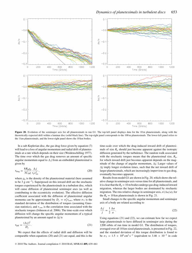
Dynamics of planetesimals in turbulent discs 653
Figure 20. Evolution of the semimajor axis for all planetesimals in run G1. The top-left panel displays data for the 10 m planetesimals, along with thetheoretically expected drift within a laminar disc (solid black line). The top-right panel corresponds to the 100 m planetesimals. The lower-left panel refers tothe 1 km planetesimals, and the lower-right panel shows the 10 km bodies.
In a sub-Keplerian disc, the gas drag force given by equation (7)will lead to a loss of angular momentum and radial drift of planetes-imals at a rate which depends on their size (Weidenschilling 1977).The time over which the gas drag removes an amount of specificangular momentum equal to � j from an embedded planetesimal isgiven by
τdrag = 8Rp�p
3CD�
�j
rpv2pg
, (20)
where �p is the density of the planetesimal material (here assumedto be 3 g cm−3). Superposed on this inward drift are the stochastictorques experienced by the planetesimals in a turbulent disc, whichwill cause diffusion of planetesimal semimajor axes (as well ascontributing to the eccentricity evolution). The effective diffusioncoefficient associated with the diffusion of planetesimal angularmomenta can be approximated by Dj = σ 2
Tτcorr, where σ T is thestandard deviation of the distribution of torques (assuming Gaus-sian statistics), and τ corr is the correlation time associated with thestochastic torques (Johnson et al. 2006). The time-scale over whichdiffusion will change the specific angular momentum of a typicalplanetesimal by an amount equal to �j is
τdiff = (�j )2
Dj
. (21)
We expect that the effects of radial drift and diffusion will becomparable when equations (20) and (21) are equal, and this is the
time-scale over which the drag-induced inward drift of planetesi-mals of size Rp should just become apparent against the isotropicdiffusion generated by the turbulence. The random walk associatedwith the stochastic torques means that the planetesimal size, Rp,for which inward drift just becomes apparent depends on the mag-nitude of the change of angular momentum, �j. Larger values of�j imply longer evolution times, such that the net inward drift oflarger planetesimals, which are increasingly impervious to gas drag,eventually becomes apparent.
Results from model G1 are shown in Fig. 20, which shows the rel-ative change in semimajor axis versus time for all planetesimals, andit is clear that the Rp = 10 m bodies undergo gas drag-induced inwardmigration, whereas the larger bodies are dominated by stochasticmigration. The rms relative change in semimajor axis, σ (�a/a), forthe Rp = 10 km planetesimals is shown in Fig. 21.
Small changes to the specific angular momentum and semimajoraxis of a body are related according to
�j
j= 1
2
�a
a. (22)
Using equations (21) and (22), we can estimate how far we expectlarge planetesimals to have diffused in semimajor axis during the1200 orbits of run time in model G1. The distribution of torques,averaged over all 10 km sized planetesimals, is presented in Fig. 22,and the standard deviation of this torque distribution is found tobe σ T = 1.5 × 108 cm2 s−2 (equivalent to 3.46 × 10⁻⁵ in code
C© 2010 The Authors. Journal compilation C© 2010 RAS, MNRAS 409, 639–661

654 R. P. Nelson and O. Gressel
Figure 21. Evolution of the rms change in semimajor axis for 10 km sizedplanetesimals, where each line is annotated with the run label.
Figure 22. Distribution of torques experienced by the 10 km sized plan-etesimals in run G1, averaged over all planetesimals. The standard deviationobtained for the distribution σ = 1.5 × 108 cm2 s−1.
units). The correlation time, τ corr, was estimated to be τ corr = 0.32orbits from the exponential decay of the ACF shown in Fig. 9 inSection 3.3.1. The diffusion coefficient, Dj, expressed in code unitsis given by Dj = 9.51 × 10⁻⁹, which leads to the prediction thata typical planetesimal located at r = 2.5 (5 au) in model G1 willdiffuse such that �a/a = 0.021. Comparing this with the value ofσ (�a/a) in Fig. 21, we see that the simulation resulted in σ (�a/a)� 0.03 after 1200 orbits, in reasonable agreement with the valuepredicted by the diffusion coefficient. The fact that the estimatedamount of diffusion is too small by a factor of ∼√
2 compared to thesimulation result indicates that the approximation to the diffusioncoefficient given by Dj = σ 2
Tτcorr is too small by a factor of �2. Thispossibly arises because of the ambiguity discussed in Section 3.3.1regarding the definition of the correlation time, but may also beaffected by sampling errors that arise from using only 25 particlesper size bin, leading to Poisson errors at the ∼20 per cent level.
We can now examine if the gas drag-induced radial drift of theRp = 10 m bodies observed in Fig. 20, and the stochastic migra-tion of all larger planetesimals, is expected. According to equa-tion (22) and Fig. 21, stochastic migration causes a relative change in
specific angular momentum �j/j = 0.015. Putting this value intoequation (20) tells us that planetesimals of size Rp � 25 metresshould radially drift due to gas drag and diffuse by a similar dis-tance. Planetesimals which are smaller than this should show stronginward drift, and larger bodies should have their evolution domi-nated by diffusion. The relative change in semimajor axes for allplanetesimals in run G1 plotted in Fig. 20 shows good agreementwith this expectation.
Changes in the mean drag-induced radial drift rate due to theturbulence can only be discerned for planetesimals of size Rp =10 m in Fig. 20, where the straight black line plotted in the top-leftpanel shows the trajectory of a planetesimal embedded in a laminardisc. Up to a time of approximately 300 orbits, the mean drift ratesof the planetesimals in the turbulent disc closely match the trajec-tory in the laminar disc. At later times, however, the trajectoriesdiverge, with the drift rates for the planetesimals in the turbulentdisc decreasing by about a factor of 3. This is not due to the effectsof stochastic forces, which earlier on in the evolution are seen tocause a dispersion of the trajectories around a mean which matchesthe laminar case closely. Instead, variations in the effective α stressparameter as a function of radius cause radial structuring of the disc,such that peaks and troughs in the mean surface density arise. Theslowing down of the radial drift observed in Fig. 20 arises when theplanetesimals enter a region of the disc in which the magnitude ofthe radial pressure gradient decreases. Thus, we observe that signif-icant changes to the radial drift of planetesimals do not occur dueto stochastic forcing, but may arise because of radial structuring ofthe disc due to spatial variations in turbulent stresses, which persistover the run times of the simulations.
If we adopt a typical disc lifetime of 5 Myr (Haisch et al. 2001),then we can estimate the amount of radial diffusion for large (Rp ≥1 km) planetesimals during the planet forming epoch. Adopting adiffusion coefficient, Dj, which gives agreement with the amount ofradial diffusion observed for 10 km-sized planetesimals in Fig. 21,equation (21) predicts �j/j = 0.3, corresponding to a 50 per centchange in the semimajor axis of a typical planetesimal located ini-tially at 5 au. Considering the relative contributions to radial driftof solid bodies from both gas drag-induced migration and diffu-sion due to the stochastic gravitational field of the disc, we haveplotted the evolution times τ drag and τ diff in Fig. 23, assuming a 30per cent change in the specific angular momentum of a planetesi-mal, using equations (20) and (21). We can see that for evolutiontimes of 5 Myr, the drag and diffusion time-scales are equal for
Figure 23. Variation of τ drag and τ diff as a function of planetesimal size.The underlying disc model is the same as in run G1.
C© 2010 The Authors. Journal compilation C© 2010 RAS, MNRAS 409, 639–661

Dynamics of planetesimals in turbulent discs 655
planetesimal size Rp � 100 m, but drag time-scales are much largerthan diffusion time-scales for larger bodies such as 1 km and 10 km-sized planetesimals. This shows that large-scale migration of largeplanetesimals over evolution times of 5 Myr will be dominated bydiffusion and not gas drag-induced inward drift.
Strong radial mixing of planetesimals at the level of �a/a = 0.5would have very significant implications for planetary formation. Inour own Solar system, for example, radial mixing of large icy plan-etesimals from beyond the snowline would substantially increasethe volatile content of the terrestrial planets, and effectively smearout the observed apparent variation in asteroid properties as a func-tion of heliocentric distance. It thus seems unlikely that such radialmixing occurred in the solar nebula, providing strong circumstantialevidence that the degree of turbulence present in model G1 was notpresent in the solar nebula during the formation of the Solar system.We explore the degree of radial mixing as a function of turbulentstrength (measured by the effective α parameter) below.
3.7.1 Planetesimal diffusion as a function of α
The rms value of the relative change in the semimajor axes for10 km sized planetesimals for various models is shown in Fig. 21.The discs in models G1 and G5 gave rise to very similar values of α
and 〈δ�/�〉, and we see that the radial diffusion rates are also verysimilar. Model G3 had a value of α = 0.017, and a correspondinglysmaller value of 〈δ�/�〉, which leads to a slower rate of diffusion.The rate of diffusion in semimajor axis is a fairly weak function ofα (see discussion below), such that it is only after a time of t ∼ 600orbits that the divergence in the diffusion rates can be detected formodels G1 and G3 in Fig. 21. Model G4 has a substantially largervalue of α = 0.101, and leads to a noticeably larger rate of diffusionof �a/a in Fig. 21.
We have fit the data for σ (�a/a) shown in Fig. 21 assuminga simple random walk model σ (�a/a) = Cσ (�a)
√t , and the
coefficients Cσ (�a) are given in Table 1. If we fit the data given inTable 1 for α and Cσ (�a) using the function Cσ (�a) = K�aα
q, thenthe best-fitting solution gives q = 0.20 and K�a = 1.70 × 10⁻³. Thisis the same power-law dependence found for the evolution of thevelocity dispersion as a function of α. This fit allows us to estimatethe amount of radial diffusion that we expect as a function of α.
3.7.2 Radial diffusion constraints on α in the solar nebula
As discussed above, large planetesimals experience only smallchanges in their angular momenta and semimajor axes due to gasdrag, assuming that they remain on approximately circular orbits.For example, a 10 km sized planetesimal orbiting at 5 au in modelG1, in the absence of turbulence, would migrate a distance of ∼4 ×10⁻³ au in 5 Myr. For such large bodies, evolution of the semimajoraxis is dominated by turbulence-induced diffusion, especially if thedisc is fully turbulent as in models G1–G5. Model G1 predicts thata typical 10 km sized planetesimal orbiting at 5 au will diffuse adistance �a � 2.5 au in 5 Myr. If this 50 per cent change in semi-major axis is applied to bodies in the asteroid belt, then this levelof diffusion is probably inconsistent with the variation in observedproperties of asteroids as a function of heliocentric distance (Gradie& Tedesco 1982; Mothe-Diniz, Carvano & Lazzaro 2003). Thesevariations would have been smeared out substantially if such a largeamount of orbital diffusion had taken place during the Solar systemformation.
The survey of how the distribution of asteroidal taxonomic typesvaries as a function of heliocentric distance presented by Gradie &Tedesco (1982) concluded that there is a systematic variation. Forthe seven taxonomic classes identified in their sample, it was sug-gested that the distribution of each peaks at a different location inthe asteroid belt, with a dispersion around this peak location of 0.5–1 au. The observed correlation between asteroidal type (assumed torelate to composition) and heliocentric distance was interpreted asbeing evidence that the asteroids were formed essentially in theirobserved locations, being subject subsequently to a relatively mod-est amount of radial mixing at the level of ∼0.5 au. The more recentsurvey of Mothe-Diniz et al. (2003) presents a more complicatedpicture in which S-type asteroids are distributed more uniformlythroughout the asteroid belt, but are none the less the dominantclass in the inner and middle belts, with the more volatile-rich C-type bodies being preferentially located in the outer belt beyond�3 au.
Radial mixing of planetesimals during planet formation is ex-pected to occur through gravitational interaction with planetaryembryos. Wetherill (1992) suggested that a population of nearlyMars-mass embryos embedded within the primordial asteroid beltcould explain the required mass depletion and radial mixing. Morerecent simulations of this effect (Petit, Morbidelli & Chambers2001; O’Brien, Morbidelli & Bottke 2007) show that radial diffu-sion of asteroids peaks at a value �a � 0.5 au, broadly consistentwith the observational constraints. In a series of related simulations,O’Brien, Morbidelli & Levison (2006) examined the formation ofterrestrial planets, and estimated the rate of water delivery to theEarth by accretion of volatile-rich material from beyond ∼2.5 au.It was found that simulations initiated with Jupiter- and Saturn-analogues on circular orbits could reasonably explain the abundanceof water on the Earth (�5 × 10⁻⁴ M⊕). Substantial radial mixingof volatile-rich planetesimals and embryos from the outer asteroidbelt, due to disc turbulence, would very likely lead to terrestrialplanets which are endowed with water and other volatiles well inexcess of what is observed.
We suggest that orbital diffusion due to turbulence which exceeds�a � 0.5 au is probably inconsistent with observations, and we nowdiscuss which value of α is consistent with �a � 0.5 au in the as-teroid belt. It should be noted, however, that using the asteroid beltas a test for dynamical mixing requires that the observed variationof properties with heliocentric distance is primordial. The recentsuggestion by Levison et al. (2009) that cometary material originat-ing from further out in the Solar system became implanted in theasteroid belt during the late heavy bombardment means we shouldtake care not to over interpret the observations, or their theoreticalimplications.
Using the approximate fit C�a = K�aα0.20, discussed in Sec-
tion 3.7.1, combined with σ (�a/a) = C�a
√t , we can estimate
which value of α should lead to an amount of diffusion which isconsistent with the above discussion. Assuming that the dispersionin asteroid properties as a function of heliocentric distance is con-sistent with diffusion generating σ (�a/a) = 0.16( ≡ 0.5/3) overa putative solar nebula lifetime of 5 Myr (Haisch et al. 2001), andnoting that K�a = 1.7 × 10⁻³ (see Section 3.7.1), we find an up-per limit for α � 5 × 10⁻⁵. Interestingly, this is very similar tothe midplane Reynolds stress obtained in shearing box simulationsof discs with dead zones (Fleming & Stone 2003; Turner, Sano &Dziourkevitch 2007; Ilgner & Nelson 2008). It would seem thatour rough estimate for the amount of diffusion which can occuras a function of α provides circumstantial evidence that the solarnebula did indeed contain a substantial dead zone in the vicinity
C© 2010 The Authors. Journal compilation C© 2010 RAS, MNRAS 409, 639–661

656 R. P. Nelson and O. Gressel
of the asteroid belt and giant planet formation region. We note,however, that caution must be used when interpreting this result.Confirmation of the variation of diffusion rate as a function of α
is required using simulations which include vertical stratificationand dead zones, and account needs to be made of the fact that thenebula mass changes significantly over a 5 Myr period. Models forthe formation of giant planets require nebula masses approximatelythree to five times larger than the MMSN (Pollack et al. 1996),which will increase the value of σ (�a/a) by a similar factor. Thedisc mass will deplete over the nebula lifetime, so that the net effectof these competing factors needs to be examined in more detail.
Taken together, the constraints on α lead to some interestingconclusions regarding the strength of turbulence in the solar neb-ula. Shearing box simulations with dead zones generate Reynoldsstresses at the midplane with α ∼ 10−5. If this stress is accompa-nied by density waves and stochastic torques with amplitudes whichfollow the scaling described in Section 3.7.1, then it becomes verydifficult to see how runaway growth could have caused rapid growthof planetary embryos via planetesimal accretion. Indeed, our resultssuggest that with α = 10−6, catastrophic disruption of 10 km sizedbodies remains possible (although this conclusion must await firmconfirmation from more realistic, vertically stratified simulations).Taken at face value, this indicates that a mechanism is requiredfor forming large bodies which avoids the need to go through therunaway growth phase, such as that suggested by Johansen et al.(2007). The existence of gradients in the chemical composition ofSolar system bodies as a function of heliocentric distance, however,is broadly consistent with a nebula model in which there exists adead zone with Reynolds stress α � 10−5. The existence of thesechemical gradients, however, is apparently inconsistent with a fullyturbulent disc model with effective α � 10−5.
3.7.3 Evolution of the eccentricity and �a/a
For small values of the eccentricity, the relation between the rmseccentricity, σ (e), and the radial velocity dispersion, σ (vr), may beapproximated as σ (e) � σ (vr)/vK, where vK is the Keplerian ve-locity. In Section 3.6.2, we showed that for the larger planetesimalswith Rp = 10 km, the radial velocity dispersion may be approxi-mated as a random walk with σ (vr) = Cσ (vr)
√t , where σ (vr) is
measured in units of the local sound speed, cs, and the Cσ (vr) valuesare listed in Table 1. Similarly, we have shown in Section 3.7.1 thatthe rms radial diffusion σ (�a/a) = Cσ (�a)
√t , where the Cσ (�a)
values are also listed in Table 1. Thus, we expect the ratio of ec-centricity changes to semimajor axis changes, σ (e)/σ (�a/a) =(H/r)Cσ (vr)/Cσ (�a). Taking the value H/r = 0.05 for the modelsG1–G4, we find that 0.34 ≤ σ (e)/σ (�a/a) ≤ 0.57, so that changesin the relative semimajor axes are similar to eccentricity changesfor larger planetesimals that are subject to stochastic gravitationalinteraction with a turbulent disc.
3.7.4 Diffusion versus type I migration of low-mass protoplanets
In addition to considering the radial drift of planetesimals due to gasdrag, and the role of stochastic torques in potentially inhibiting thisinward drift, we can also consider the effect that these stochastictorques might have on the type I migration of low-mass planets(Nelson & Papaloizou 2004; Nelson 2005). We have ascertainedabove that bodies undergoing diffusion due to stochastic torquesmay change their semimajor axes by 50 per cent over a disc lifetimeof 5 Myr. Using the type I migration formula from Tanaka, Takeuchi
& Ward (2002) for a disc model with properties which are thesame as model G1, we note that planets with mpl/M� = 3.5 ×10⁻⁷ will migrate a distance equal to 50 per cent of their initialsemimajor axis (assumed to be 5 au) via type I migration over 5 Myr.This indicates that direct competition between type I migration andstochastic migration will only prevent the large-scale migration ofplanetary bodies with masses similar to that of Mars over suchnebula lifetimes. It should be noted, however, that the possibleradial structuring of protoplanetary discs by turbulence due to spatialvariations in α (possibly due to a dead zone) may provide a meansof preventing inward drift due to the operation of corotation torques(Masset 2001; Masset et al. 2006).
3.8 Migration of planetesimals – local model
The local shearing box approximation that we have adopted in thiswork does not include the effect of a radial pressure gradient in mod-ifying the orbital angular velocity of the gas. Consequently, the gasand embedded bodies orbit at the same mean angular velocity, andplanetesimals do not undergo radial migration due to gas drag inter-action with a sub-Keplerian disc. Large planetesimals, whose inter-action with the gas disc is gravity dominated, experience stochasticgravitational forces that cause diffusion of the semimajor axes (orequivalently, the guiding centres of the particle epicycles). Smallerbodies, whose evolution is dominated by gas drag, similarly diffuseradially due to the stochastic gas drag forces. We discuss both ofthese regimes below.
3.8.1 Diffusion of gravity dominated bodies
As with the larger planetesimals discussed in Section 3.7 for theglobal models, the larger planetesimals in the shearing box simu-lations undergo radial diffusion due to the stochastic gravitationalforces they experience. The deviation in the positions of the guidingcentres of particles from their initial values is denoted as �x (mea-sured in units of the local scaleheight H), and we plot the standarddeviation of this quantity for the gravity-only particles (set ‘G’) inFig. 24. As with the global simulations, the evolution of �x dis-plays random walk behaviour. As is illustrated by the fitted curveand error bounds in Fig. 24, the random walk can reasonably be
Figure 24. Dispersion in the radial displacement �x for a swarm of particlessubject to the gas gravity alone. The time evolution follows a random walkas reasonably well described by the given relation.
C© 2010 The Authors. Journal compilation C© 2010 RAS, MNRAS 409, 639–661
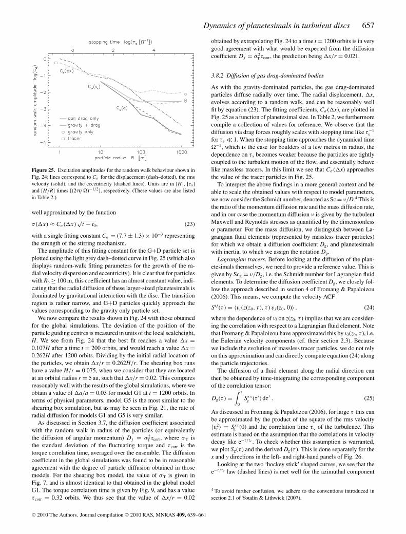
Dynamics of planetesimals in turbulent discs 657
Figure 25. Excitation amplitudes for the random walk behaviour shown inFig. 24; lines correspond to Cσ for the displacement (dash–dotted), the rmsvelocity (solid), and the eccentricity (dashed lines). Units are in [H], [cs]and [H/R] times [(2π/�)−1/2], respectively. (These values are also listedin Table 2.)
well approximated by the function
σ (�x) ≈ Cσ (�x)√
t − t0, (23)
with a single fitting constant Cσ = (7.7 ± 1.3) × 10−3 representingthe strength of the stirring mechanism.
The amplitude of this fitting constant for the G+D particle set isplotted using the light grey dash–dotted curve in Fig. 25 (which alsodisplays random-walk fitting parameters for the growth of the ra-dial velocity dispersion and eccentricity). It is clear that for particleswith Rp ≥ 100 m, this coefficient has an almost constant value, indi-cating that the radial diffusion of these larger-sized planetesimals isdominated by gravitational interaction with the disc. The transitionregion is rather narrow, and G+D particles quickly approach thevalues corresponding to the gravity only particle set.
We now compare the results shown in Fig. 24 with those obtainedfor the global simulations. The deviation of the position of theparticle guiding centres is measured in units of the local scaleheight,H. We see from Fig. 24 that the best fit reaches a value �x =0.107H after a time t = 200 orbits, and would reach a value �x =0.262H after 1200 orbits. Dividing by the initial radial location ofthe particles, we obtain �x/r = 0.262H/r. The shearing box runshave a value H/r = 0.075, when we consider that they are locatedat an orbital radius r = 5 au, such that �x/r = 0.02. This comparesreasonably well with the results of the global simulations, where weobtain a value of �a/a = 0.03 for model G1 at t = 1200 orbits. Interms of physical parameters, model G5 is the most similar to theshearing box simulation, but as may be seen in Fig. 21, the rate ofradial diffusion for models G1 and G5 is very similar.
As discussed in Section 3.7, the diffusion coefficient associatedwith the random walk in radius of the particles (or equivalentlythe diffusion of angular momentum) Dj = σ 2
Tτcorr, where σ T isthe standard deviation of the fluctuating torque and τ corr is thetorque correlation time, averaged over the ensemble. The diffusioncoefficient in the global simulations was found to be in reasonableagreement with the degree of particle diffusion obtained in thosemodels. For the shearing box model, the value of σ T is given inFig. 7, and is almost identical to that obtained in the global modelG1. The torque correlation time is given by Fig. 9, and has a valueτ corr = 0.32 orbits. We thus see that the value of �x/r = 0.02
obtained by extrapolating Fig. 24 to a time t = 1200 orbits is in verygood agreement with what would be expected from the diffusioncoefficient Dj = σ 2
Tτcorr, the prediction being �x/r = 0.021.
3.8.2 Diffusion of gas drag-dominated bodies
As with the gravity-dominated particles, the gas drag-dominatedparticles diffuse radially over time. The radial displacement, �x,evolves according to a random walk, and can be reasonably wellfit by equation (23). The fitting coefficients, Cσ (�x), are plotted inFig. 25 as a function of planetesimal size. In Table 2, we furthermorecompile a collection of values for reference. We observe that thediffusion via drag forces roughly scales with stopping time like τ−1
s
for τ s � 1. When the stopping time approaches the dynamical time�−1, which is the case for boulders of a few metres in radius, thedependence on τ s becomes weaker because the particles are tightlycoupled to the turbulent motion of the flow, and essentially behavelike massless tracers. In this limit we see that Cσ (�x) approachesthe value of the tracer particles in Fig. 25.
To interpret the above findings in a more general context and beable to scale the obtained values with respect to model parameters,we now consider the Schmidt number, denoted as Sc = ν/D.4 This isthe ratio of the momentum diffusion rate and the mass diffusion rate,and in our case the momentum diffusion ν is given by the turbulentMaxwell and Reynolds stresses as quantified by the dimensionlessα parameter. For the mass diffusion, we distinguish between La-grangian fluid elements (represented by massless tracer particles)for which we obtain a diffusion coefficient Dg, and planetesimalswith inertia, to which we assign the notation Dp.
Lagrangian tracers. Before looking at the diffusion of the plan-etesimals themselves, we need to provide a reference value. This isgiven by Scg = ν/Dg, i.e. the Schmidt number for Lagrangian fluidelements. To determine the diffusion coefficient Dg, we closely fol-low the approach described in section 4 of Fromang & Papaloizou(2006). This means, we compute the velocity ACF
Sij (τ ) = 〈vi(z(z0, τ ), τ ) vj (z0, 0)〉 , (24)
where the dependence of vi on z(z0, τ ) implies that we are consider-ing the correlation with respect to a Lagrangian fluid element. Notethat Fromang & Papaloizou have approximated this by vi(z0, τ ), i.e.the Eulerian velocity components (cf. their section 2.3). Becausewe include the evolution of massless tracer particles, we do not relyon this approximation and can directly compute equation (24) alongthe particle trajectories.
The diffusion of a fluid element along the radial direction canthen be obtained by time-integrating the corresponding componentof the correlation tensor:
Dg(τ ) =∫ τ
0Sxx
g (τ ′) dτ ′ . (25)
As discussed in Fromang & Papaloizou (2006), for large τ this canbe approximated by the product of the square of the rms velocity〈v2
x 〉 = Sxxg (0) and the correlation time τ c of the turbulence. This
estimate is based on the assumption that the correlations in velocitydecay like e−τ/τc . To check whether this assumption is warranted,we plot Sg(τ ) and the derived Dg(τ ). This is done separately for thex and y directions in the left- and right-hand panels of Fig. 26.
Looking at the two ‘hockey stick’ shaped curves, we see that thee−τ/τc law (dashed lines) is met well for the azimuthal component
4 To avoid further confusion, we adhere to the conventions introduced insection 2.1 of Youdin & Lithwick (2007).
C© 2010 The Authors. Journal compilation C© 2010 RAS, MNRAS 409, 639–661

658 R. P. Nelson and O. Gressel
Table 2. Random walk-amplitudes Cσ describing the stochastic excitation (as depicted in Fig. 24) of the dispersion within an ensemble. Values areobtained for the displacement �x, the rms radial velocity dispersion, vx, and the eccentricity e. With the exception of the first column, the applicability
of the functional form Cσ (t − t0)1/2 is of course limited to the time interval before saturation is reached (see Figs 13 and 14).
Gravity only Gravity + drag Drag force only Tracer[(2π/�)−1/2] × 10 m 100 m 1 km 10 m 100 m 1 km
Cσ (�x) [10−2 H] 0.77 ± 0.13 11.4 ± 0.02 0.95 ± 0.11 0.94 ± 0.10 7.71 ± 0.03 0.44 ± 0.12 0.01 ± 0.18 56.5 ± 0.01Cσ (vx ) [10−3 cs] 3.53 ± 0.03 45.9 ± 3.75 2.54 ± 0.36 2.79 ± 0.04 45.1 ± 3.10 0.46 ± 0.01 0.03 ± 0.00 —Cσ (e) [10−3 H/R] 2.77 ± 0.53 — 2.57 ± 0.04 2.58 ± 0.01 — 0.85 ± 0.01 0.03 ± 0.00 —
Figure 26. Velocity ACFs Sxxg (left-hand panel) and S
yyg (right-hand panel)
for massless tracers. From the ACFs (black lines, LHS axes), we obtain time-integrated diffusion coefficients Dg(t) (grey line, RHS axes). The fits Sg ∼e−τ/τc (dashed black) result in corresponding diffusion profiles (dashedgrey) which agree for τ � 2π/�. For τ � 1, Dg can be approximated bythe given theoretical estimate (dash–dotted line).
(right-hand panel), whereas there is considerable tension for theradial direction (left-hand panel). Note that the time domain haslogarithmic scaling, which implies that the deviation in the shapeof the curve cannot be accounted for by changing the fit param-eter τ c. Tentatively, an exponential decay law can be restored viatransformation to a generalized time variable τ → τα with α � 0.7– we however leave it open whether the observed issue bears anyrelevance at the current stage of modelling.
Our fitted correlation times are τ (x)c = 0.92 �−1 = 0.15×2π�−1
and τ (y)c = 1.12 �−1 = 0.18 × 2π�−1. The obtained numbers are
in fact very close to the value of 0.15 orbits, reported in Fromang &Papaloizou (2006). This supports the notion that τ c is characteristicfor MRI-typical Mach numbers and only weakly depends on theactual amplitude of the turbulent stresses.
The relation from equation (25) is illustrated by solid grey linesin Fig. 26, which represent the diffusion ‘constant’ Dg as a functionof time. For comparison, we also plot the diffusion profile corre-sponding to the fitted solution (dashed grey lines). These curvesreasonably approximate the τ dependence of Dg for τ � 2π/�.Note, however, that the fitted amplitude is somewhat smaller thanthe rms velocities and the curves saturate at a lower value. Thismeans that the real correlation functions have a (stochastic) tail thatleads to a further growth in Dg for τ � 2π/�.
For times sufficiently greater than the correlation time of the flow,the diffusion coefficient approaches a constant value approximatedby τ c 〈v2〉 � 0.035 as indicated by dash–dotted lines in the twopanels of Fig. 26. In accordance with a recent study by Madarassy& Brandenburg (2010), the observed anisotropy in the streamwiseand cross-stream directions is rather weak.
Translated into a Schmidt number, we yield a value of Scg � 1.6,which is considerably lower than the ratio between the Maxwelland Reynolds stress, which fluctuates between 3 and 4. Our value
Figure 27. Velocity ACF Sp(τ ) (solid black line) for particles with radiusR = 5 m. The exponential decay is now modulated by epicyclic oscillationsand can be fitted via a function ∼ cos(2πτ�−1) e−τ/τc (white dashed line).The envelope (dotted lines) is assumed to be relevant for the diffusion of theguiding centre.
is a factor of about 2 smaller than the Eulerian value for verticaldiffusion found by Fromang & Papaloizou (2006). Schmidt numbersobtained for small particles are usually inferred to be of the order ofunity (Johansen & Klahr 2005; Turner et al. 2006), and our resultsare compatible with this.
A Schmidt number of the order of unity implies that small dustgrains that are strongly coupled to the gas will diffuse over large dis-tances during protostellar disc lifetimes. Observations of crystallinesilicates embedded in circumstellar discs at significant distancesfrom their host stars, where temperatures are too low to explain insitu crystallization of amorphous grains (van Boekel et al. 2004),suggest that turbulent diffusion may indeed be responsible for trans-porting grains from the hot inner regions of discs to the cooler outerregions. It remains to be demonstrated, however, in a global, turbu-lent disc model, whether or not a substantial number of grains canbe transported outwards against the net inward mass accretion flowon to the star.
Particles with inertia. Unlike massless tracers, real particles aresubject to the additional body forces in the rotating coordinateframe. Consequently, this leads to the excitation of epicyclic oscil-lations. In the case of the Keplerian rotation, the associated angularfrequency κ is identical with the local rotation rate �. The ACFfor a perfect epicyclic oscillation is then simply proportional tocos(2πτ�−1). This means that velocities are maximally correlatedif they are apart by a full period, and anti-correlated in between.
In general, the particles’ motion will, however, deviate from aperfect epicycle – or, in other words, the defining elements of themotion will change stochastically. With both the eccentricity andthe position of the guiding centre fluctuating, the coherence ofthe motion is lost for larger times. This is illustrated in Fig. 27,where we plot the velocity ACF for particles of size Rp = 5 m.The epicyclic nature of the particle motion is clearly seen in the
C© 2010 The Authors. Journal compilation C© 2010 RAS, MNRAS 409, 639–661

Dynamics of planetesimals in turbulent discs 659
Table 3. Time-scales and Schmidt numbers Scp =αss csH/Dp for the diffusion of the guiding centresof heavy particles on excited epicyclic orbits.
Rp = 1 m 2 m 5 m 10 m 20 m
τ s (�−1) 0.23 0.91 5.71 22.8 91.4τ c (�−1) 0.68 1.59 5.74 16.7 46.4τ s/τ c 2.96 1.74 1.01 0.73 0.51Scp 4.22 27.5 45.3 96.4 182.
Figure 28. Attempt to determine the Schmidt number Sc = Dg/Dp for thediffusion of the guiding centres. The diffusion coefficient is estimated viaDp � τc〈v2
gc〉, where vgc is obtained by smoothing over the epicycles (solidlines). An alternative estimate (open squares) is derived independently viathe coefficients C2
σ (�x) in Table 2 – note that these do not depend on anyform of smoothing.
sinusoidal modulation of Sp. If integrated over time, the ‘diffusion’process would rather resemble a shaking motion than a randomwalk.
As a result, this renders the direct integration approach illus-trated in Fig. 26 difficult. Taking the excellent agreement with thefunctional dependence ∼ cos(2πτ�−1) e−τ/τc , we however conjec-ture that the diffusive part of the overall motion can be recoveredfrom the exponential envelope function (dotted line in Fig. 27). InTable 3, we report this correlation time as a function of particleradius Rp and compare5 it to the stopping time τ s. The ratio τ c/τ s
is about unity for Rp = 5 m and roughly scales with the square-rootof the radius.
Given we can obtain a good estimate for the rms velocity ofthe guiding centres, we can then compute Dp � τc〈v2
gc〉. Looking atFig. 11, it seems less than straightforward to deconvolve the randommotion of the guiding centre from the overall motion, especiallysince the amplitude of the epicycles changes on comparable time-scales. As a first attempt, we simply smooth out the oscillationsapplying a box-car filter in time. The thus derived Schmidt numberSc = Dg/Dp as a function of particle size is plotted in Fig. 28 forvarious values of the filter size.
If we omit the smoothing, the results (although not strictly cor-rect) reflect the kinetic energy in the epicyclic mode itself. In thiscase, the gradual decoupling of the particles implies that 〈v2〉 de-creases while τ c increases accordingly. Interestingly, this leavesthe overall particle diffusion rate unchanged. If we increase thefilter size, the epicyclic motion is attenuated and the size depen-dence gradually becomes steeper. Reasonable convergence is ob-
5 The ratio τ s/τ c should not be confused with the Stokes number St = τ s/τ e
which measures the particle coupling with respect to the eddy velocity.
tained when the filter size approaches the critical value, equal to theepicyclic period. In Table 3, we list the corresponding numbers.
Note that already for metre-sized objects the particle diffusivityis reduced relative to Lagrangian tracers. We attribute this to theeffect that part of the kinetic energy is absorbed in ordered epicyclicmotion and is thus not available for particle diffusion (cf. section 3.2in Youdin & Lithwick 2007). The partial slippage of the particlesthrough the gas as a result of weaker drag acceleration also causesthe particle guiding centre velocities to be reduced relative to thefluid turbulent velocities.
It might be seen as a deficiency of the approach that it dependson the proper choice of a box-car filter function. To reinforce thevalidity of the derived Schmidt numbers, we therefore provide anindependent estimate from the squares of the coefficients Cσ (�x)from Fig. 25. Defining the growing spread in the particles positionwith time, these can similarly be interpreted as a diffusion constant.For consistency, we have also checked that the fit constants Cσ (�x)do not change significantly, when the epicyclic part of the motionis smoothed. Considering that this second estimate solely relies onpositions while the original one is derived from velocity correla-tions, the agreement seen in Fig. 28 (where we plot the differentestimates for the Schmidt number) is quite striking.
4 C O N C L U S I O N S
We have presented results from both local and global MHD simu-lations which examine the evolution of planetesimals and bouldersof different size embedded in turbulent protoplanetary disc models.The main aims of this work are to: determine the magnitude of thevelocity dispersion which is excited in a planetesimal swarm; de-termine the rate of radial diffusion of the planetesimals; determineunder which conditions broad agreement is obtained in the resultsfrom local shearing box simulations and global disc simulations.
We find that the magnitude of density fluctuations, and the asso-ciated stochastic forces experienced by embedded planetesimals, issensitive to the dimensions of shearing box models. This appears tobe related to the fact that accurate modelling of the excitation andnon-linear steepening of spiral density waves requires boxes whichare elongated in the azimuthal direction (Heinemann & Papaloizou2009b). The two-point correlation function for the perturbed surfacedensity also shows that coherent structures stretched by a distance�6H are a common feature of MHD turbulence in discs, indicatingthat shearing boxes in excess of this length-scale are required toprevent the premature truncation of the gravitational field whichresults from these structures. In addition to the magnitude of thestochastic torques being dependent on the box size, we also foundthat the correlation time of the fluctuating torques also depends onthe box size and aspect ratio, with smaller boxes generating shortercorrelation times. This is apparently due to the ability of waves topropagate across the box on multiple occasions due to the periodicboundary conditions employed, combined with the rate at whichthey shear past the planet due to the background flow. Shearingboxes with dimensions 4H × 16H × 2H were found to provideconverged results which agree well with the results from globalsimulations.
We find that both global simulations and local shearing box sim-ulations predict that rapid excitation of planetesimal random ve-locities is expected in fully turbulent disc models whose local sur-face densities are similar to the MMSN. A model whose turbulentstresses generate α = 0.035 leads to rapid growth of the radial ve-locity dispersion, σ (vr), via a random walk, such that after 1200orbits at 5 au σ (vr) = 200 m s−1. A model with weaker turbulence
C© 2010 The Authors. Journal compilation C© 2010 RAS, MNRAS 409, 639–661

660 R. P. Nelson and O. Gressel
(α = 0.017) gave rise to σ (vr) = 166 m s−1 over the same evolutiontime. These random velocities are much larger than either the escapevelocities from planetesimals with sizes 1 or 10 km or the catas-trophic disruption thresholds for collisions between bodies of sim-ilar size (Benz & Asphaug 1999; Stewart & Leinhardt 2009), sug-gesting that planetesimal collisions occurring in fully turbulent discssimilar to those considered in this paper will result in the destructionof the planetesimals. We find that the expected equilibrium velocitydispersion for 10 km sized planetesimals scales weakly with theturbulent stress parameter such that σ (vr) = Kvrα
0.2. Extrapolationof the simulation results presented in this paper to low values of α
suggests that even with α = 10−6, bodies with size 10 km are likelyto have random velocities which will cause catastrophic disruptionduring mutual collisions. Values of σ (vr) small enough to allow run-away growth of planetesimals to occur will be even more difficult toachieve. For smaller bodies, which are more tightly coupled to thegas via gas drag, we find that the equilibrium velocity dispersiondecreases, and reaches a minimum of σ (vr) � 20 m s−1 for bodiesof size 50 m in a disc with α = 0.035. For smaller bodies than thesethe increasing influence of gas drag causes the velocity dispersion toincrease with decreasing size, and boulders with Rp = 1 m developrandom velocities which closely match the turbulent gas motions.
In addition to driving the growth of the velocity dispersion, orequivalently the eccentricity, the stochastic forces experienced bythe planetesimals cause them to diffuse radially through the disc.For large planetesimals with Rp = 10 km, radial drift through thedisc due to gas drag occurs very slowly, and their radial motionis expected to be dominated by diffusion caused by the stochasticgravitational field of the turbulent disc. Indeed, after a putativedisc lifetime of 5 Myr, the rms relative change in semimajor axis,σ (�a/a), for a planetesimal swarm located at 5 au in a disc withα = 0.035 will be 50 per cent, which would have been sufficientto cause large-scale migration of the small body populations of theSolar system during its formation. The fact that such large-scalemigration of large planetesimals does not appear to have happenedallows us to put constraints on the strength of α in the solar nebula.A value of α � 10−5 would lead to a more reasonable σ (�a/a) �0.1, consistent with the notion that the solar nebula had a dead zonein the region where planet formation took place.
Smaller planetesimals with Rp = 10–100 m are expected to un-dergo large-scale radial drift due to gas drag, and this is observedin our simulations. The migration rate of 10 m size bodies in theturbulent discs, relative to that expected for an equivalent laminardisc model, is found to be very similar. Migration in turbulent discsis found to be slower by a factor of approximately 2–3, and thisis due to radial structuring of the disc’s density profile, creatingregions where the pressure gradient (and hence rotational velocityprofile) is modified.
There have been a number of previous studies of the dynamicalevolution of planetary bodies embedded in turbulent discs. Nelson& Papaloizou (2004) examined the torques experienced by low-mass planets and suggested that random walk behaviour for suchbodies should be expected, as has been observed in this paper.Nelson (2005) examined the orbital evolution of planets embeddedin turbulent discs, with particular emphasis on the semimajor axisand eccentricity changes. The strength of the turbulence in thatmodel was somewhat weaker than considered in this paper (α �5 × 10⁻³), although the disc model was somewhat more massive,and in general it was found that the response of embedded bodiesto the stochastic forcing was stronger in that study, with largerchanges in semimajor axis and eccentricity being observed. Theprimary reason for this discrepancy appears to be the fact that a
persistent vortex formed in the disc model considered by Nelson(2005). Such vortices were also reported in the work of Fromang &Nelson (2005), and interaction between embedded bodies and suchstructures can lead to significant modification of the semimajor axesand excitation of eccentricity. The models presented in this paperdo not have such vortex features, but during the early stages of thisproject disc models with lower values of α were found to generatesuch flow features quite readily. One possibility is that global discmodels which are close to the limits of resolving the MRI generatesubstantial variations in α as a function of radius, which in turngenerate localized pressure maxima which are particularly proneto the formation of vortices (Hawley 1987; Lovelace et al. 1999).Models with smaller values of the plasma β parameter have strongerfield strengths and thus resolve the MRI more easily, and in additionthe stronger fields may act to inhibit vortex formation through theaction of local magnetic stresses. We have considered these modelsin this paper.
Yang et al. (2009) recently considered the evolution of plan-etesimal swarms using non-stratified shearing box simulations. Theplanetesimals in that study experienced the fluctuating gravitationalfield of the disc, but did not experience gas drag forces. Althoughrandom walk behaviour of the particles in that study was observed,in general it was found to be significantly weaker than we reporthere, and one conclusion reached by these authors is that turbulenceis unlikely to cause the catastrophic disruption of planetesimals. Theprimary reason for this appears to be the fact that most simulationsperformed by Yang et al. (2009) used shearing boxes with 2H ×2H × 2H. Test calculations with larger boxes presented in that pa-per indicated a strong increase in the response of the particles to theturbulence forcing as a function of increasing box size, suggestingthat the main reason for the discrepancy between the results is dueto this effect.
Ida et al. (2008) recently considered the evolution of planetesi-mals embedded in turbulent protoplanetary discs by means of N-body simulations combined with a prescription for planetesimalstirring based on the work of Laughlin et al. (2004). In basic agree-ment with the results we have presented in this paper, they showthat turbulence leads to the excitation of a large velocity dispersion,which is likely to cause catastrophic disruption of planetesimalsrather than growth following mutual collisions, for a wide range ofturbulent strengths.
The simulations we have presented here use the simplest possiblenumerical set-up: ideal MHD in non-stratified disc models. In afuture paper we will present the results of a similar study usingvertically stratified models with and without dead zones. This futurestudy will tell us whether we need to examine new paradigms for therapid growth of planetesimals, or whether instead runaway growthcan indeed occur within a dead zone of an otherwise turbulentprotoplanetary disc.
AC K N OW L E D G M E N T S
OG thanks Sebastien Fromang for discussions on improving thenumerical scheme and providing his spectral analysis tools. RPNthanks Alessandro Morbidelli and Bill Bottke for discussions aboutthe radial mixing of asteroids. This work used the NIRVANA-III codedeveloped by Udo Ziegler at the Astrophysical Institute Potsdam.All computations were performed on the QMUL HPC facility, pur-chased under the SRIF initiative. RPN and OG acknowledge thehospitality of the Isaac Newton Institute for Mathematical Sciences,where most of the work presented in this paper was completed dur-ing the ‘Dynamics of Discs and Planets’ research programme.
C© 2010 The Authors. Journal compilation C© 2010 RAS, MNRAS 409, 639–661

Dynamics of planetesimals in turbulent discs 661
RE FERENCES
Adams F. C., Bloch A. M., 2009, ApJ, 701, 1381Adams F. C., Laughlin G., Bloch A. M., 2008, ApJ, 683, 1117Armitage P. J., 1998, ApJ, 501, L189Bai X., Stone J. M., 2010, preprint (astro-ph/1005.4982)Balbus S. A., Hawley J. F., 1991, ApJ, 376, 214Balbus S. A., Hawley J. F., 2006, ApJ, 652, 1020Balsara D. S., Meyer C., 2010, preprint (astro-ph/1003.0018)Balsara D. S., Spicer D. S., 1999, J. Comput. Phys., 149, 270Balsara D. S., Tilley D. A., Rettig T., Brittain S. D., 2009, MNRAS, 397,
24Baruteau C., Lin D. N. C., 2010, ApJ, 709, 759Benz W., Asphaug E., 1999, Icarus, 142, 5Bodo G., Mignone A., Cattaneo F., Rossi P., Ferrari A., 2008, A&A, 487, 1Davis S. W., Stone J. M., Pessah M. E., 2010, ApJ, 713, 52de Val-Borro M. et al., 2006, MNRAS, 370, 529Fleming T., Stone J. M., 2003, ApJ, 585, 908Flock M., Dzyurkevich N., Klahr H., Mignone A., 2010, A&A, 516, 26Fromang S., Nelson R. P., 2005, MNRAS, 364, L81Fromang S., Papaloizou J., 2006, A&A, 452, 751Fromang S., Papaloizou J., 2007, A&A, 476, 1113Fromang S., Papaloizou J., Lesur G., Heinemann T., 2007, A&A, 476, 1123Gammie C. F., 2001, ApJ, 553, 174Gardiner T. A., Stone J. M., 2005, J. Comput. Phys., 205, 509Gardiner T. A., Stone J. M., 2008, J. Comput. Phys., 227, 4123Goldreich P., Ward W. R., 1973, ApJ, 183, 1051Gradie J., Tedesco E., 1982, Sci, 216, 1405Gressel O., Ziegler U., 2007, Comput. Phys. Communications, 176, 652Haisch K. E. Jr, Lada E. A., Lada C. J., 2001, ApJ, 553, L153Hawley J. F., 1987, MNRAS, 225, 677Hawley J. F., 2001, ApJ, 554, 534Hawley J. F., Stone J. M., 1995, Comput. Phys. Communications, 89, 127Hawley J. F., Gammie C. F., Balbus S. A., 1995, ApJ, 440, 742Hayashi C., 1981, Progress Th. Phys. Suppl., 70, 35Heinemann T., Papaloizou J. C. B., 2009a, MNRAS, 397, 52Heinemann T., Papaloizou J. C. B., 2009b, MNRAS, 397, 64Ida S., Makino J., 1993, Icarus, 106, 210Ida S., Guillot T., Morbidelli A., 2008, ApJ, 686, 1292Ilgner M., Nelson R. P., 2008, A&A, 483, 815Johansen A., Klahr H., 2005, ApJ, 634, 1353Johansen A., Oishi J. S., Low M., Klahr H., Henning T., Youdin A., 2007,
Nat, 448, 1022Johansen A., Youdin A., Klahr H., 2009, ApJ, 697, 1269Johnson E. T., Goodman J., Menou K., 2006, ApJ, 647, 1413Johnson B. M., Guan X., Gammie C. F., 2008, ApJS, 177, 373Kokubo E., Ida S., 1998, Icarus, 131, 171Laughlin G., Steinacker A., Adams F. C., 2004, ApJ, 608, 489Lesur G., Longaretti P.-Y., 2007, MNRAS, 378, 1471Levison H. F., Bottke W. F., Gounelle M., Morbidelli A., Nesvorny D.,
Tsiganis K., 2009, Nat, 460, 364Lovelace R. V. E., Li H., Colgate S. A., Nelson A. F., 1999, ApJ, 513, 805Madarassy E. J. M., Brandenburg A., 2010, Phys. Rev. E, 82, 016304Masset F., 2000, A&AS, 141, 165
Masset F. S., 2001, ApJ, 558, 453Masset F. S., 2002, A&A, 387, 605Masset F. S., Morbidelli A., Crida A., Ferreira J., 2006, ApJ, 642, 478Miniati F., 2010, J. Comput. Phys., 229, 3916Miyoshi T., Kusano K., 2005, J. Comput. Phys., 208, 315Mothe-Diniz T., Carvano J. M. A., Lazzaro D., 2003, Icarus, 162, 10Nelson R. P., 2005, A&A, 443, 1067Nelson R. P., Papaloizou J. C. B., 2003, MNRAS, 339, 993Nelson R. P., Papaloizou J. C. B., 2004, MNRAS, 350, 849O’Brien D. P., Morbidelli A., Levison H. F., 2006, Icarus, 184, 39O’Brien D. P., Morbidelli A., Bottke W. F., 2007, Icarus, 191, 434Ogihara M., Ida S., Morbidelli A., 2007, Icarus, 188, 522Oishi J. S., Mac Low M., Menou K., 2007, ApJ, 670, 805Papaloizou J. C. B., Nelson R. P., 2003, MNRAS, 339, 983Papaloizou J. C. B., Nelson R. P., Snellgrove M. D., 2004, MNRAS, 350,
829Petit J., Morbidelli A., Chambers J., 2001, Icarus, 153, 338Pollack J. B., Hubickyj O., Bodenheimer P., Lissauer J. J., Podolak M.,
Greenzweig Y., 1996, Icarus, 124, 62Press W. H., Teukolsky S. A., Vettering W. T., Flannery B. P., 1996, Numer-
ical Recipes in Fortran 90: The Art of Scientific Computing. CambridgeUniversity Press, Cambridge
Rafikov R. R., 2004, AJ, 128, 1348Regev O., Umurhan O. M., 2008, A&A, 481, 21Rein H., Papaloizou J. C. B., 2009, A&A, 497, 595Shakura N. I., Syunyaev R. A., 1973, A&A, 24, 337Sicilia-Aguilar A., Hartmann L. W., Briceno C., Muzerolle J., Calvet N.,
2004, AJ, 128, 805Stewart S. T., Leinhardt Z. M., 2009, ApJ, 691, L133Stone J. M., Gardiner T. A., 2010, ApJS, 189, 142Stone J. M., Norman M. L., 1992, ApJS, 80, 753Tanaka H., Takeuchi T., Ward W. R., 2002, ApJ, 565, 1257Turner N. J., Sano T., 2008, ApJ, 679, L131Turner N. J., Willacy K., Bryden G., Yorke H. W., 2006, ApJ, 639, 1218Turner N. J., Sano T., Dziourkevitch N., 2007, ApJ, 659, 729van Boekel R. et al., 2004, Nat, 432, 479van Leer B., 1977, J. Comput. Phys., 23, 276Ward W. R., 1997, Icarus, 126, 261Weidenschilling S. J., 1977, MNRAS, 180, 57Wetherill G. W., 1992, Icarus, 100, 307Wetherill G. W., Stewart G. R., 1993, Icarus, 106, 190Winters W. F., Balbus S. A., Hawley J. F., 2003, ApJ, 589, 543Yang C., Mac Low M., Menou K., 2009, ApJ, 707, 1233Youdin A., Johansen A., 2007, ApJ, 662, 613Youdin A. N., Goodman J., 2005, ApJ, 620, 459Youdin A. N., Lithwick Y., 2007, Icarus, 192, 588Ziegler U., 2004, J. Comput. Phys., 196, 393Ziegler U., 2008, Comput. Phys. Communications, 179, 227Ziegler U., Yorke H. W., 1997, CoPhC, 101, 54
This paper has been typeset from a TEX/LATEX file prepared by the author.
C© 2010 The Authors. Journal compilation C© 2010 RAS, MNRAS 409, 639–661