A Possible Correlation between the Gaseous Drag Strength and Resonant Planetesimals in Planetary...
34
a r X i v : a s t r o p h / 0 6 1 0 6 6 8 v 1 2 3 O c t 2 0 0 6 A Possible Correlation between the Gaseous Drag Strength and Resonant Planetesimals in Planetary Systems Ing-Guey Jiang 1 and Li-Chin Yeh 2 1 Department of Physics, National Tsing-Hua University, Hsin-Chu, Taiwan 2 Department of Applied Mathematics, National Hsinchu University of Education, Hsin-Chu, Taiwan Received ; accepted
Transcript of A Possible Correlation between the Gaseous Drag Strength and Resonant Planetesimals in Planetary...

8/14/2019 A Possible Correlation between the Gaseous Drag Strength and Resonant Planetesimals in Planetary Systems
http://slidepdf.com/reader/full/a-possible-correlation-between-the-gaseous-drag-strength-and-resonant-planetesimals 1/34
a r X i v : a s t
r o - p h / 0 6 1 0 6 6 8 v 1
2 3 O c t 2 0 0 6
A Possible Correlation between the Gaseous Drag Strength and
Resonant Planetesimals in Planetary Systems
Ing-Guey Jiang1 and Li-Chin Yeh2
1 Department of Physics,
National Tsing-Hua University, Hsin-Chu, Taiwan
2 Department of Applied Mathematics,
National Hsinchu University of Education, Hsin-Chu, Taiwan
Received ; accepted

8/14/2019 A Possible Correlation between the Gaseous Drag Strength and Resonant Planetesimals in Planetary Systems
http://slidepdf.com/reader/full/a-possible-correlation-between-the-gaseous-drag-strength-and-resonant-planetesimals 2/34
– 2 –
ABSTRACT
We study the migration and resonant capture of planetesimals in a planetary
system consisting of a gaseous disc analogous to the primordial solar nebula
and a Neptune-like planet. Using a simple treatment of the drag force we find
that planetesimals are mainly trapped in the 3:2 and 2:1 resonances and that
the resonant populations are correlated with the gaseous drag strength in a
sense that the 3:2 resonant population increases with the stronger gaseous drag,
but the 2:1 resonant population does not. Since planetesimals can lead to the
formation of larger bodies similar to asteroids and Kuiper Belt Objects, the
gaseous drag can play an important role in the configuration of a planetary
system.
Subject headings: circumstellar matter – planetary systems – stellar dynamics

8/14/2019 A Possible Correlation between the Gaseous Drag Strength and Resonant Planetesimals in Planetary Systems
http://slidepdf.com/reader/full/a-possible-correlation-between-the-gaseous-drag-strength-and-resonant-planetesimals 3/34
– 3 –
1. Introduction
The discovery of more than 160 planets orbiting other stars, extra-solar planets,
opened a window of astronomy, which could eventually provide insight to understanding
the fundamental questions about our own Solar System. Most of these extra-solar planets
(exoplanets) were detected by the measurements of stellar radial velocities of their host star
via the Doppler effect and several more recent detected exoplanets were discovered through
the transit events. For example, the OGLE project has detected 5 transit exoplanets
(Konacki et al. 2003, Bouchy et al. 2005), and the TrES team (using 10 cm telescopes) has
discovered one transit planet (Alonso et al. 2004). All of the above 6 exoplanets were later
confirmed by spectroscopic follow-up. Future observations using both methods will lead to
the discoveries of additional systems, thereby improving the statistical significance of the
population.
Among the many interesting properties exhibited by these planetary systems are the
large range of masses, orbital periods and orbital eccentricities (Jiang et al. 2006). In
particular, the relations between the orbital periods of different planets have been noted
and are usually connected with the mean motion resonances. As an example of extra-solar
multiple planetary systems which show the resonances, Ji et al. (2003) confirmed that
the 55 Cancri planetary system is indeed in the 3:1 mean motion resonance by both the
numerical simulations and secular theory. The GJ 876 and HD 82943 planetary systems are
probably in 2:1 resonance as studied by Laughlin & Chambers (2001), Kinoshita & Nakai
(2001), Gozdziewski & Maciejewski (2001) and also Ji et al. (2002). Moreover, the periods
of small bodies in the Solar System such as asteroids and Kuiper Belt Objects (KBOs) are
also seen to have similar connections with resonances. Thus, such types of dynamics may
also play a role in the configuration of KBOs.
On the other hand, it has been shown that discs can affect the orbital evolution of

8/14/2019 A Possible Correlation between the Gaseous Drag Strength and Resonant Planetesimals in Planetary Systems
http://slidepdf.com/reader/full/a-possible-correlation-between-the-gaseous-drag-strength-and-resonant-planetesimals 4/34
– 4 –
test particles within planetary systems (Jiang & Yeh 2004a, 2004b; Yeh & Jiang 2005).
In particular, Jiang & Yeh (2004c) proposed a possible model of resonant capture for
proto-KBOs driven by the gaseous drag, finding that many test particles can be captured
into the 3:2 resonance, consistent with the observational results (Luu & Jewitt 2002).
To ensure that the gaseous drag influences the dynamics of planetesimals, sufficient
gas must be present (about 0.01M ⊙ as suggested in Nagasawa et al. 2000) when the
planetesimals are already formed. It is likely that molecular gas is present around the
nearby star epsilon Eridani as found by Greaves et al. (1998), however, only an upperlimit of 0.4 Earth masses in molecular gas is inferred from CO observations. This is to be
compared to the primordial solar nebula where the minimum-mass solar nebula is about
0.026 M ⊙.
Although there is evidence for a small amount of gas present in planetary systems,
there may have been much more gas in the past. The km-sized planetesimals representing
proto-asteroids were formed and likely influenced by the gaseous drag. During the above
process, the gaseous component is gradually depleted from a more massive primordial
nebula to the current limited molecular gas.
Whether the above scenario is viable would be related to the formation time-scale
of km-sized planetesimals and the depletion time-scale of the gaseous discs. Cuzzi et al.
(1993) argued that 10-100 km sized objects can be formed in about 106 years. Furthermore,
observations by Kenyon & Hartmann (1995), Haisch et al. (2001) show that at the age of
about 106 years, most low-mass stars are surrounded by the optically thick discs. However,
by the age of 107 years, no such discs are detected. It is therefore possible that there is
a phase in the evolution of the system where planetesimals are already formed while the
gaseous disc is not yet depleted. We investigate this phase to examine the effect of gaseous
drag for the planetesimal dynamics in this paper.

8/14/2019 A Possible Correlation between the Gaseous Drag Strength and Resonant Planetesimals in Planetary Systems
http://slidepdf.com/reader/full/a-possible-correlation-between-the-gaseous-drag-strength-and-resonant-planetesimals 5/34
– 5 –
Since the km-sized planetesimals will grow into asteroids, KBOs or even planets, their
distribution and orbital evolution are extremely important for understanding the history
of planetary systems. Based on a disc model analogous to the primordial solar nebula,
we study the resonant capture of planetesimals under the influence of a gaseous disc for a
given planetary system. In particular, we study the possibility for correlations between the
gaseous drag strength and the resonant populations and examine the possible parameter
space for which the drag-induced resonant capture could explain the resonant populations
of a planetary system.
We present our model and assumptions in § 2. § 3 describes the evolution of
planetesimals and the stability tests. Finally, we discuss the results and conclude in the last
section.
2. The Model
We consider the motion of a test particle influenced by the gravitational force from the
central star, a planet and the proto-stellar disc. This disc, which is mainly composed of gas,
exerts a drag on the planet and the test particles. These test particles are envisioned to
represent planetesimals such as proto-asteroids and proto-KBOs. We assume that the mass
of central star µ1 = 1M ⊙, and the planet’s mass is taken to be similar to the Neptune’s
mass, i.e. µ2 = 5 × 10⁻⁵M ⊙. We assume the test particle represents a planetesimal with
a radius about 10 km, with a mass assumed to be about µ3 = 4.3 × 10⁻¹⁵M ⊙ (when the
density is similar with the Pluto’s). The coordinates of the central star, the planet and the
planetesimal are (0, 0), (x, y) and (ξ, η), respectively.
In this paper, we consider the general situation that the planet is free to move on any
non-circular orbit.

8/14/2019 A Possible Correlation between the Gaseous Drag Strength and Resonant Planetesimals in Planetary Systems
http://slidepdf.com/reader/full/a-possible-correlation-between-the-gaseous-drag-strength-and-resonant-planetesimals 6/34
– 6 –
2.1. The Units
In this paper, the unit of mass is M ⊙ and the unit of length is 30 AU. Since we set the
gravitational constant G = 1, the total simulation time, 3.8×10⁵, which would correspond to
107 years. All simulations start from t = 0 and terminate at t = tend = 123200π ∼ 3.8× 10⁵.
2.2. The Equations of Motion
In this paper, we only consider the coplanar case, so all motions are in a two
dimensional plane. The equations of motion are
d2xdt2
= −µ1xr3− α
µ2
dxdt− vx
ρN −
dV N
drxr
,
d2y
dt2= −µ1
y
r3− α
µ2
dy
dt− vy
ρN −
dV N
dr
y
r,
d2ξ
dt2= −µ1
ξ
r31
+ µ2x−ξ
r32
− αµ3
(dξdt− vξ)ρT −
dV T dr1
ξ
r1,
d2η
dt2= −µ1
η
r31
+ µ2y−η
r32
− αµ3
(dηdt− vη)ρT −
dV T dr1
η
r1,
(1)
where
r2 = x2 + y2, (2)
r21 = ξ2 + η2, (3)
r22
= (x− ξ)2 + (y − η)2. (4)
The equations of motion in terms of x and y describe the planet’s orbit and the equations of
ξ and η give the orbit of a test particle. In Eq. (1), V N is the disc potential for the planet.
In other words, we define that V N = V (r) to be the disc potential at the planet’s location
(x, y) where r is given by Eq. (2) and ρN = ρ(r) is the disc density at the planet’s location.
Similarly, V T = V (r1) is the disc potential at the test particle’s location (ξ, η) where r1 is
given in Eq. (3) and ρT = ρ(r1) is the disc density at the location of the test particle.
The disc is represented by an annulus with inner edge ri and outer edge ro, where ri
and ro are assumed to be constants. We choose ri = 1/5, ro = 5/3 in this paper. Since we

8/14/2019 A Possible Correlation between the Gaseous Drag Strength and Resonant Planetesimals in Planetary Systems
http://slidepdf.com/reader/full/a-possible-correlation-between-the-gaseous-drag-strength-and-resonant-planetesimals 7/34
– 7 –
set the unit of length to be 30 AU, ri corresponds to the location where the Jupiter was
formed approximately and ro corresponds to the outer edge of the Kuiper Belt. Thus, our
choice of inner and outer edges of the gaseous disc is based on the possible properties of the
proto-solar nebula.
The density profile of the disc is taken to be of the form ρ(r) = c/r p, where r is the
radial coordinate as in Eq. (2), c is a constant completely determined by the total mass of
the disc and p is a natural number. In this paper, we set p = 2 based on the theoretical
work by Lizano & Shu (1989). This assumption is consistent with one of the models of theVega debris disc (Su et al. 2005). Hence, the total mass of the disc is
M d =
2π
0
rori
ρ(r′)r′dr′dφ = 2πc(ln ro − ln ri). (5)
In this paper, the disc mass is assumed to be M d = 0.01, which is the same order as the
minimum-mass solar nebula (0.026 M ⊙). It is also consistent with the observations by
Beckwith et al. (1990) in which the discs have masses ranging from 0.001 to 1 M ⊙. The
disc’s gravitational potential and force can be calculated by elliptic integrals as in Jiang &Yeh (2004b).
In Eq. (1), the Keplerian velocity of the gaseous material in the ξ direction is
vξ = −
µ1r1
sin θT and in the η direction is vη =
µ1r1
cos θT , where θT = tan−1(η/ξ).
Similarly, vx = −
µ1r
sin θN and vy =
µ1r
cos θN , where θN = tan−1(y/x).
2.3. The Drag
In this system, we include the effect of the drag force from the gaseous disc. There
are various forms for the drag force that could be employed. For example, Murray (1994)
considered a general drag force per unit mass of the form:
F = kVg, (6)

8/14/2019 A Possible Correlation between the Gaseous Drag Strength and Resonant Planetesimals in Planetary Systems
http://slidepdf.com/reader/full/a-possible-correlation-between-the-gaseous-drag-strength-and-resonant-planetesimals 8/34
– 8 –
where k < 0, V is the particle’s velocity in the inertial frame, and g is a scalar function of
its position and velocity.
On the other hand, the aerodynamic friction force per unit mass is given by (Fitzpatrick
1970, Fridman & Gorkavyi 1999)
F =1
2mC DAρV 2r , (7)
where C D is the drag coefficient, m and A are the particle’s mass and cross-section, ρ is the
gaseous density, and V r is the magnitude of particle’s velocity relative to the gas.
The Epstein drag force per unit mass has also been adopted (see Youdin & Shu 2002,
Youdin & Chiang 2004) and is given by
F =4π
3mρgcgva2, (8)
where ρg is the mass density of gas and cg is the gas sound speed. The particle’s mass and
size are m and a respectively. The relative velocity between a particle and gas is v.
Our disc is mainly composed of gas and we wish to approximate the disc’s gaseous drag
acting on the planetesimals and planets. Motivated by the above expressions for the drag,
we employ a unified formula which we use for both planetesimals and the planet. Thus, we
assume that the drag force per unit mass is:
F = −αρ
mV, (9)
where α is assumed to be a constant, V is the particle’s velocity relative to the Keplerian
motion of the gaseous disc, and ρ is the gas density.
Although our drag differs from the Epstein drag, we can see that α plays the role of
4πcga2/3 of Epstein drag. To obtain an estimate of the value of α, we (i) use Eq.(2) of
Youdin & Chiang (2004) to calculate cg, (ii) use the radius of our planetesimal particle,

8/14/2019 A Possible Correlation between the Gaseous Drag Strength and Resonant Planetesimals in Planetary Systems
http://slidepdf.com/reader/full/a-possible-correlation-between-the-gaseous-drag-strength-and-resonant-planetesimals 9/34
– 9 –
10 km, to be the value of a, and find that 4πcga2/3 is about 8 × 10⁻¹⁶. We, thus, define
αE ≡ 8× 10⁻¹⁶. Due to the simple treatment of the disc drag and the uncertainty in α, we
adopt 3 different values of α: αE , 5αE , and 25αE .
For the planet, the drag force in x direction is −(α/µ2)(dx/dt−vx)ρN and thus this term
appears in the first equation of Eq. (1). Similarly, there is a term −(α/µ2)(dy/dt− vy)ρN
appears in the second equation of Eq. (1).
For the planetesimals, the drag force in the ξ and η directions are −(α/µ3)(dξ/dt−vξ)ρT
and −(α/µ3)(dη/dt− vη)ρT in the third and fourth equation of Eq. (1), respectively.
2.4. The Simulations
A number of planetesimals (300) are randomly distributed in a belt region
1.1 ≤ r ≤ 1.8 with a uniform number density, where r is the radial coordinate. Assuming
that one planetesimal is located at (ξ, η), then we set its initial velocity (voξ, voη) to
be voξ = −(
1/r1)sin θT and voη = (
1/r1)cos θT , where θT = tan−1(η/ξ). Thus, the
planetesimals are initially in circular motion.
To study the outcome of different drag strengths, we adopt 3 different values of the
drag coefficient in our simulations. That is, α = αE in model A, α = 5αE in model B and
α = 25αE in model C.
The planet is always located at (1, 0) initially, and was set in circular motion initially
for models A, B, and C. However, in order to test the influence of the planet’s orbital
eccentricity, we also consider a model (D) in which the planet moves on an initial eccentric
orbit of e = 0.3 with drag coefficient chosen to be α = 5αE .
To study the resonance captures, the orbital semi-major axis and eccentricity for all the

8/14/2019 A Possible Correlation between the Gaseous Drag Strength and Resonant Planetesimals in Planetary Systems
http://slidepdf.com/reader/full/a-possible-correlation-between-the-gaseous-drag-strength-and-resonant-planetesimals 10/34
– 10 –
planetesimals and planet are calculated. To make it clear, x∗, y∗ represent the coordinates
of any particle. From Murray & Dermott (1999), we have
r2∗ = x2
∗+ y2
∗,
v2 =
dx∗dt
2
+
dy∗dt
2
.
Let h2 = (x∗dy∗dt− y∗
dx∗dt
)2, then semi-major axis a and eccentricity e are defined by
a =
2
r∗−
v2
µ1
−1
, (10)
e =
1− h2
µ1a. (11)
Based on the formula in Murray & Dermott (1999) and Fitzpatrick (1970), the 2:1 resonant
argument φ2:1 and 3:2 resonance argument φ3:2 are also calculated as
φ3:2 = 3λt − 2λN − ωt, (12)
φ2:1 = 2λt − λN − ωt, (13)
where λt is the mean longitude of a planetesimal’s orbit, λN is the mean longitude of the
planet’s orbit and ωt is the longitude of pericentre of a planetesimal’s orbit.
The number of particles in a particular resonance at time ti is defined to be the total
number of particles with the difference between the maximum and minimum resonance
arguments less than 180o during ti−1 < t < ti. We set t0 = 0, ti = ti−1 + 800π, where
i = 1, 2, ..., 154.
3. Numerical Results
3.1. Evolution of Planetesimals
The evolution of planetesimals on the x − y plane in the simulation of model A is
illustrated in Fig. 1. The panel labelled 0 in Fig. 1 shows the initial positions of all 300

8/14/2019 A Possible Correlation between the Gaseous Drag Strength and Resonant Planetesimals in Planetary Systems
http://slidepdf.com/reader/full/a-possible-correlation-between-the-gaseous-drag-strength-and-resonant-planetesimals 11/34
– 11 –
planetesimals. Based on this representation, it is difficult to discern the change in the
distribution until the 9th panel. However, specifically it can be seen in the histograms of
particle number versus the radial distance reveal the variation more clearly (see Fig. 2). In
the 2nd panel of Fig. 2, a gap starts to develop and this gap becomes deeper and wider
in the following panels. Finally, the gap encompasses the range from 1.5 to 1.7 after the
8th panel. The gap can also been seen in panels 10 and 11 of Fig. 1 and separates the
planetesimal distribution into two rings. The outer ring (from r = 1.7 to r = 1.8) is thinner
than the inner one (from r = 1.1 to r = 1.5) as one can see from Fig. 1 and 2.
In Fig. 3, we plot the final planetesimal distribution of model A in the a− e plane on
the left panel and also the color contour of it on the right panel. There is a population
with nearly circular orbits from a = 1.7 to a = 1.8. They are the main population of the
outer ring of Fig. 1 and 2 as one can estimate the total number from the color bar. From
both panels and also the color bar, we find that some planetesimals are associated with 2:1,
3:2, 7:5, 4:3, 5:4, 6:5 resonances and that there are more planetesimals in 3:2 (at a = 1.33)
than those in 2:1 resonance (at a = 1.6). However, in order to confirm whether a given
planetesimal is captured into a particular resonance, the particular resonance argument
has to be calculated during the whole simulation. Because the influence of the first order
resonance, 2:1 and 3:2, are much stronger than the others, we calculate the 2:1 and 3:2
resonance arguments, i.e. φ2:1 and φ3:2. Fig. 3 also shows that there is a non-resonant
population (from a = 1.4 to a = 1.5) with nearly circular orbits. This population, together
with all the resonant population between 1.1 and 1.5, become the main population of the
inner wider ring of Fig. 1 and 2. The orbital eccentricities of the 2:1 resonant population
are larger and thus these planetesimals have wider range in semi-major axis. Although this
wider range might cover both rings and also the gap of Fig. 1 and 2, the number of this
population is small so that they do not change the distribution.

8/14/2019 A Possible Correlation between the Gaseous Drag Strength and Resonant Planetesimals in Planetary Systems
http://slidepdf.com/reader/full/a-possible-correlation-between-the-gaseous-drag-strength-and-resonant-planetesimals 12/34
– 12 –
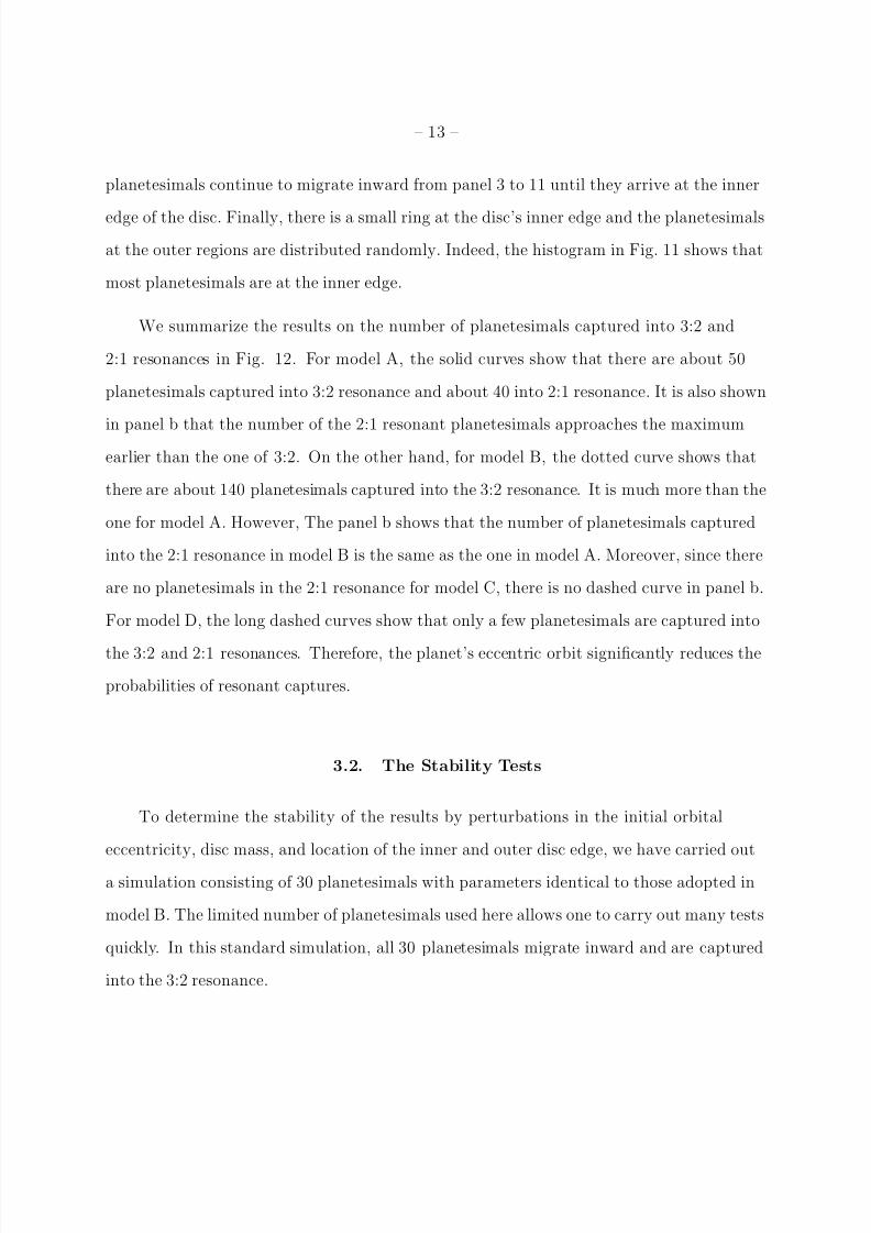
The evolution of planetesimals’ distribution for model B is plotted in Fig. 4. The
evolution proceeds more rapidly than in model A. This could be due to a larger drag force
for this model. For example, in the 2nd panel, there is already a gap in the belt. The
planetesimals continue to migrate inward and the gap becomes wider as shown in panels
3 and 4. In the 5th panel, the planetesimals are seen to distribute into two parts, i.e. an
inner ellipse and an outer ring. The inner ellipse precesses slowly starting from panel 6
until the end of the simulation. This behaviour is confirmed in the histograms in Fig. 5 as
the gap begins to form in panel 2. The inward migration is also evident as particle number
increases between r = 1 and r = 1.5.
It can be seen in Fig. 6 that some planetesimals associated with the 2:1 and 3:2
resonances cluster around a = 1.6 and a = 1.33. All the planetesimals associated with the
3:2 resonance have almost exactly the same semi-major axes and, moreover, there is no
other non-resonant planetesimals around a = 1.33, explaining why the inner ellipse is so
thin in Fig. 4.
In model C, the largest drag force is considered. The planetesimals’ inward migrations
are so fast that there is already a gap in the 1st panel of Fig. 7. A clear inner ellipse
is formed in panel 2 and it precesses slightly at the following panels. With that small
precession, the whole distribution seems to be a steady state. The histograms of Fig. 8 also
confirm the existence of the gap. We point out that there are no planetesimals in the 2:1
resonance for this model (see Fig. 9).
Although the planet’s orbital eccentricity is taken to be zero initially, its eccentricity is
about 0.02 during the simulations for models A, B, and C. In model D, the strength of the
drag force is assumed to be moderate, i.e. the same as the one in model B, but the initial
orbital eccentricity of the planet is 0.3. Due to the drag, the inward migrations are still
significant and the gap immediately appears in the 1st and 2nd panel of Fig. 10. However,
8/14/2019 A Possible Correlation between the Gaseous Drag Strength and Resonant Planetesimals in Planetary Systems
http://slidepdf.com/reader/full/a-possible-correlation-between-the-gaseous-drag-strength-and-resonant-planetesimals 13/34
– 13 –
planetesimals continue to migrate inward from panel 3 to 11 until they arrive at the inner
edge of the disc. Finally, there is a small ring at the disc’s inner edge and the planetesimals
at the outer regions are distributed randomly. Indeed, the histogram in Fig. 11 shows that
most planetesimals are at the inner edge.
We summarize the results on the number of planetesimals captured into 3:2 and
2:1 resonances in Fig. 12. For model A, the solid curves show that there are about 50
planetesimals captured into 3:2 resonance and about 40 into 2:1 resonance. It is also shown
in panel b that the number of the 2:1 resonant planetesimals approaches the maximumearlier than the one of 3:2. On the other hand, for model B, the dotted curve shows that
there are about 140 planetesimals captured into the 3:2 resonance. It is much more than the
one for model A. However, The panel b shows that the number of planetesimals captured
into the 2:1 resonance in model B is the same as the one in model A. Moreover, since there
are no planetesimals in the 2:1 resonance for model C, there is no dashed curve in panel b.
For model D, the long dashed curves show that only a few planetesimals are captured into
the 3:2 and 2:1 resonances. Therefore, the planet’s eccentric orbit significantly reduces the
probabilities of resonant captures.
3.2. The Stability Tests
To determine the stability of the results by perturbations in the initial orbital
eccentricity, disc mass, and location of the inner and outer disc edge, we have carried out
a simulation consisting of 30 planetesimals with parameters identical to those adopted in
model B. The limited number of planetesimals used here allows one to carry out many tests
quickly. In this standard simulation, all 30 planetesimals migrate inward and are captured
into the 3:2 resonance.

8/14/2019 A Possible Correlation between the Gaseous Drag Strength and Resonant Planetesimals in Planetary Systems
http://slidepdf.com/reader/full/a-possible-correlation-between-the-gaseous-drag-strength-and-resonant-planetesimals 14/34
– 14 –
To check the stability of the orbital evolution to the initial orbital eccentricities of
planetesimals, a simulation was performed in which all planetesimals have initial orbital
eccentricities e = 0.01 with all other settings remaining the same as the standard one.
These 30 planetesimals migrate inward of which 27 are captured into the 3:2 resonance.
Because the difference with the standard case is only 3 planetesimals, which is one order of
magnitude less than the total number, 30, we conclude that the system is stable in terms of
the initial orbital eccentricities of planetesimals. For the results in which 300 planetesimals
are used, we are confident that the result would be similar if the planetesimals’ initial
orbital eccentricities were changed slightly.
To test the stability in terms of the disc mass, i.e. the value of M d, we ran two
simulations, one with M d = 0.009 and another one with M d = 0.011 while keep all other
settings the same as the standard one. Note that M d = 0.01 in the standard case. For
both simulations, all the 30 planetesimals migrate inward and are captured into the 3:2
resonance. Thus, the system is stable to perturbations in the disc mass.
To check the stability in terms of the location of the disc’s edges, i.e. the value of ri
and ro, 4 simulations were carried out with ri = 1/5−0.01, ri = 1/5 + 0.01, ro = 5/3−0.01,
ro = 5/3 + 0.01, while all other settings remaining the same as the standard case. All the 30
planetesimals migrate inward and are captured into the 3:2 resonance for all 4 simulations.
Hence, the system is stable in terms of perturbations to the disc inner and outer edges.
4. Discussions and Conclusions
In this paper, we have investigated the effect of different strengths of the gaseous
drag on the resonant capture into the 3:2 and 2:1 resonances. For a small drag force as
in model A, there are about 17 percent of planetesimals captured into the 3:2 resonance

8/14/2019 A Possible Correlation between the Gaseous Drag Strength and Resonant Planetesimals in Planetary Systems
http://slidepdf.com/reader/full/a-possible-correlation-between-the-gaseous-drag-strength-and-resonant-planetesimals 15/34
– 15 –
and about 13 percent into the 2:1 resonance. For a moderate drag force as in model B,
the fraction of planetesimals captured into 2:1 is still about 13 percent but the fraction for
the 3:2 resonance increases to 47 percent. When a stronger drag force is used as in model
C, the fraction of planetesimals captured into the 3:2 resonance greatly increases up to
about 60 percent. In contrast, the number for the 2:1 resonance becomes zero. Therefore,
the numerical results of the resonant capture process reveal that it is very sensitive to the
strength of the gaseous drag. Since the planetesimals are captured into resonances during
their inward migrations, the stronger drag increases the speed of inward migration, so,
equivalently, the resonant population in capture processes is correlated with the speed of
inward migration.
For a model in which the planet has an initially eccentric orbit, less than 3 percent of
the planetesimals are trapped into the 3:2 and 2:1 resonances. Hence, the assumption of a
large finite eccentricity nearly destroys the possibility of resonant captures.
To understand the difference between the 3:2 and 2:1 resonant captures, there are
mainly two possibilities:
(1) the details of capture processes for the 3:2 and 2:1 resonances are fundamentally
different, strongly depend on the migration speed of planetesimals.
(2) under our assumptions, there are more planetesimals passing the 3:2 resonant region
during the simulations, so that more planetesimals are captured into the 3:2 resonance,
even though the capture probabilities for 3:2 and 2:1 resonances are similar.
In order to understand whether the 2nd explanation is correct, we estimate the capture
probability for both the 3:2 and 2:1 resonances. Let us assume that the potential candidates
to be captured into the 2:1 resonance are those planetesimals initially located between the
outer edge (r = 1.8) and the 2:1 resonant region (about r = 1.6). Since there are 300

8/14/2019 A Possible Correlation between the Gaseous Drag Strength and Resonant Planetesimals in Planetary Systems
http://slidepdf.com/reader/full/a-possible-correlation-between-the-gaseous-drag-strength-and-resonant-planetesimals 16/34
– 16 –
planetesimals uniformly distributed in the region 1.1 ≤ r ≤ 1.8, the potential number of
planetesimals to be captured into the 2:1 resonance is
300×(1.82 − 1.62)
(1.82 − 1.12)∼ 100.
For model A, the total number of planetesimals captured into 2:1 is about 40, and the
capture probability for the 2:1 resonance is about 40%.
The potential candidates to be captured into the 3:2 resonance, on the other hand,
are those planetesimals initially located between the 2:1 resonant region (about r = 1.6)and 3:2 resonant region (about r = 1.33) plus those planetesimals initially located out of
r = 1.6 but not captured into the 2:1 resonance, so the potential number of planetesimals
to be captured into the 3:2 resonance is
300×(1.62 − 1.332)
(1.82 − 1.12)+ 60 ∼ 177.
Thus, the capture probability for the 3:2 resonance is about 50/177 = 28%, which is smaller
than the one for the 2:1 resonance.
For model B, the capture probability for the 2:1 resonance is still about 40%, however
the total number of planetesimals captured into the 3:2 resonance increases significantly up
to about 140. This could be due to the fact that some planetesimals initially located out of
r = 1.6 but not captured into the 2:1 resonance are also captured into the 3:2 resonance in
time due to fast inward migrations.
Since the potential number of planetesimals to be captured into the 3:2 resonance is
again 177, the capture probability for the 3:2 resonance is 140/177, which is about 79%.
Therefore, not only is the number of planetesimals passing into the 3:2 resonant region
larger than the one for the 2:1 resonance, but also that the capture probability of the 3:2
resonance is larger than that of the 2:1 resonance.

8/14/2019 A Possible Correlation between the Gaseous Drag Strength and Resonant Planetesimals in Planetary Systems
http://slidepdf.com/reader/full/a-possible-correlation-between-the-gaseous-drag-strength-and-resonant-planetesimals 17/34
– 17 –
For the largest gaseous drag considered (model C), the speed of inward migration is
highest and even more planetesimals are in the 3:2 resonance. However, in this case, the
number of particles in the 2:1 resonance vanishes.
From the above analysis for models A, B, and C, we confirm that the details of the
3:2 and 2:1 resonant capture are fundamentally different. As discussed in Peale (1976) and
Murray & Dermott (1999), the resonant relations are determined by the influence of the
planet on the planetesimals. In particular, during the conjunctions, the net tangential force
experienced by the planetesimal is key because it can change the planetesimal’s angularmomentum.
In the case when the planet moves on a circular orbit and the planetesimals are
assumed to move on eccentric orbits, there is no net tangential force if the conjunctions
occur exactly at the peri-center or apo-center. When the conjunctions occur at any other
point on the orbit, the symmetry is destroyed, and thus, there is net tangential force. For
a dense population of planetesimals moving on the same eccentric orbit, the net tangential
force would cause about half of them to gain angular momentum and another half to lose
angular momentum. If all these planetesimals were driven to migrate inwards due to the
drag, (1) those which gain angular momentum would expand their orbits a bit and could
be captured into the resonance, (2) those which lose angular momentum would continue
to migrate inward. Since (a) the planetesimals might move on different orbits and (b) the
exact locations of the repeated conjunctions are not known, it is difficult to estimate the
capture probability.
The symmetry is further destroyed when the planet moves on the orbit with large
eccentricity 0.3. As a result, it is more difficult for those conjunctions which lead to
planetesimals gaining angular momentum to take place repeatedly. Thus, there are few
planetesimals captured into the resonances in model D.

8/14/2019 A Possible Correlation between the Gaseous Drag Strength and Resonant Planetesimals in Planetary Systems
http://slidepdf.com/reader/full/a-possible-correlation-between-the-gaseous-drag-strength-and-resonant-planetesimals 18/34
– 18 –
For the Kuiper Belt in the outer Solar System, objects are known to occupy the 3:2
and 2:1 resonant regions. The conventional mechanism explaining these resonances relies
on the resonant capture by an outwardly migrating Neptune with a migration time-scale
τ = 2 × 10⁶ years (Malhotra 1995). This migration was assumed to start in the late
stages of the genesis of the Solar System when the formation of the gas giant planet was
largely complete, the solar nebula had lost its gaseous component, and the evolution was
dominated by the gravitational interactions. However, this mechanism is based on an
assumption of pure radial orbital migrations. The generality of this mechanism is unclear
if a more realistic orbit of Neptune were chosen. As shown by the numerical simulations
in Thommes et al. (1999) and the analytic calculations in Yeh & Jiang (2001), Neptune’s
orbital eccentricity shall not be zero during the outward migration. Because Neptune is
currently moving on a circular orbit, a massive disc is needed to circularize Neptune’s orbit
if the outward migration did happen.
On the other hand, our results show that the drag-induced resonant capture can
explain the existence of objects in both 3:2 and 2:1 resonances, but the ratio of these
two populations will depend on the gaseous drag strength. The similarity between the
conventional picture and our mechanism reflects the fact that both captures are due to the
relative motions between the planet and the small bodies. The main difference is the causes
of the relative motions.
Finally, our results (model D) also show that the resonant capture occurs provided that
the planet’s orbital eccentricity is not too large. This result could place some constrainton the possible orbital history of the planet. For example, from this point of view, in the
conventional picture, Neptune will be able to capture the KBOs into the resonances only
when its eccentricity is reduced to be smaller than 0.3. This further constrains the orbital
history and the timing of Neptune’s migration if it did significantly contribute on the

8/14/2019 A Possible Correlation between the Gaseous Drag Strength and Resonant Planetesimals in Planetary Systems
http://slidepdf.com/reader/full/a-possible-correlation-between-the-gaseous-drag-strength-and-resonant-planetesimals 19/34
– 19 –
resonant capture of 3:2 and 2:1 resonant KBOs.
Acknowledgment
We acknowledge the anonymous referee’s many good suggestions. We especially thank
Prof. R. Taam for his efforts in improving the presentation. We are grateful to the National
Center for High-performance Computing for computer time and facilities.
This work is supported in part by the National Science Council, Taiwan, underIng-Guey Jiang’s Grants: NSC 94-2112-M-008-010 and also Li-Chin Yeh’s Grants: NSC
94-2115-M-134-002.

8/14/2019 A Possible Correlation between the Gaseous Drag Strength and Resonant Planetesimals in Planetary Systems
http://slidepdf.com/reader/full/a-possible-correlation-between-the-gaseous-drag-strength-and-resonant-planetesimals 20/34
– 20 –
REFERENCES
Alonso, R., Brown, T. M., Torres, G., Latham, D. W., Sozzetti, A., Mandushev, G.,
Belmonte, J. A., Charbonneau, D., Deeg, H. J., Dunham, E. W., O’Donovan, F. T.,
Stefanik, R. P. 2004, ApJ, 613, L153
Beckwith, S. V. W., Sargent, A. I., Chini, R. S., Guesten, R. 1990, AJ, 99, 924
Bouchy, F., Udry, S., Mayor, M., Moutou, C., Pont, F., Iribarne, N., da Silva, R., Ilovaisky,
S., Queloz, D., Santos, N., Segransan, D., Zucker, S. 2005, A&A, submitted,astro-ph/0510119
Cuzzi, J. N., Dobrovolskis, A. R., Champney, J. M. 1993, Icarus, 106, 102
Fitzpatrick, P. M. 1970, Principles of Celestial Mechanics, (New York: Academic Press)
Fridman, A. M., Gorkavyi, N. N. 1999, Physics of Planetary Rings, (Berlin, Heidelberg:
Springer-Verlag)
Gozdziewski, K., Maciejewski, A. J. 2001, ApJ, 563, L81
Greaves, J. S., Holland, W. S., Moriarty-Schieven, G., Jenness, T., Dent, W. R. F.,
Zuckerman, B., McCarthy, C., Webb, R. A., Butner, H. M., Gear, W. K., Walker,
H. J. 1998, ApJ, 506, L133
Haisch, K. E., Lada, E. A., Lada, C. J. 2001, ApJ, 553, L153
Hatzes, A. P., Cochran, W. D., McArthur, B., Baliunas, S. L., Walker, G. A. H., Campbell,
B., Irwin, A. W., Yang, S., Kurster, M., Endl, M., Els, S., Butler, R. P., Marcy, G.
W. 2000, ApJ, 544, L145
Ji, J., Kinoshita, H., Liu, L., Li, G. 2003, ApJ, 585, L139

8/14/2019 A Possible Correlation between the Gaseous Drag Strength and Resonant Planetesimals in Planetary Systems
http://slidepdf.com/reader/full/a-possible-correlation-between-the-gaseous-drag-strength-and-resonant-planetesimals 21/34
– 21 –
Ji, J., Li, G., Liu, L. 2002, ApJ, 572, 1041
Jiang, I.-G., Yeh, L.-C. 2004a, AJ, 128, 923
Jiang, I.-G., Yeh, L.-C. 2004b, Int. J. Bifurcation and Chaos, 14, 3153
Jiang, I.-G., Yeh, L.-C. 2004c, MNRAS, 355, L29
Jiang, I.-G., Yeh, L.-C., Hung, W.-L., Yang, M.-S. 2006, MNRAS, 370, 1379
Kenyon, S. J., Hartmann, L. 1995, ApJS, 101, 117
Kinoshita, H., Nakai, H. 2001, PASJ, 53, L25
Konacki, M., Torres, G., Jha, S., Sasselov, D. D. 2003, Nature, 421, 507
Laughlin, G., Chambers, J. 2001, ApJ, 551, L109
Lizano, S., Shu, F. H. 1989, ApJ, 342, 834
Luu, J. X., Jewitt, D. C. 2002, ARAA, 40, 63
Malhotra, R. 1995, AJ, 110, 420
Murray, C. D. 1994, Icarus, 112, 465
Murray, C. D. & Dermott, S. F. 1999, Solar System Dynamics, (Cambridge: Cambridge
University Press)
Nagasawa, M., Tanaka, H., Ida, S. 2000, AJ, 119, 1480
Peale, S. J. 1976, Annual Review of Astronomy and Astrophysics, 14, 215
Su, K. Y. L. et al. 2005, ApJ, 628, 487
Thommes, E. W., Duncan, M. J., Levison, H. F. 1999, Nature, 402, 635

8/14/2019 A Possible Correlation between the Gaseous Drag Strength and Resonant Planetesimals in Planetary Systems
http://slidepdf.com/reader/full/a-possible-correlation-between-the-gaseous-drag-strength-and-resonant-planetesimals 22/34
– 22 –
Yeh, L.-C., Jiang, I.-G. 2001, ApJ, 561, 364
Yeh, L.-C., Jiang, I.-G. 2005, Proceeding of the 9th Asian-Pacific Regional IAU Meeting
(APRIM), in press
Youdin, A. N., Chiang, E. I. 2004, ApJ, 601, 1109
Youdin, A. N., Shu, F. H. 2002, ApJ, 580, 494
This manuscript was prepared with the AAS LATEX macros v4.0.

8/14/2019 A Possible Correlation between the Gaseous Drag Strength and Resonant Planetesimals in Planetary Systems
http://slidepdf.com/reader/full/a-possible-correlation-between-the-gaseous-drag-strength-and-resonant-planetesimals 23/34
– 23 –
Fig. 1.— The model A: the evolution of particle distributions in the x− y plane. The time
between successive panels corresponds to 11200π.

8/14/2019 A Possible Correlation between the Gaseous Drag Strength and Resonant Planetesimals in Planetary Systems
http://slidepdf.com/reader/full/a-possible-correlation-between-the-gaseous-drag-strength-and-resonant-planetesimals 24/34
– 24 –
0
20
40
60
0
20
40
60
0
20
40
60
0 0.5 1 1.5 2
0
20
40
60
0 0.5 1 1.5 2 0 0.5 1 1.5 2
Fig. 2.— The model A: the histograms of particle distributions in the radial coordinate.
The time between successive panels corresponds to 11200π.

8/14/2019 A Possible Correlation between the Gaseous Drag Strength and Resonant Planetesimals in Planetary Systems
http://slidepdf.com/reader/full/a-possible-correlation-between-the-gaseous-drag-strength-and-resonant-planetesimals 25/34

8/14/2019 A Possible Correlation between the Gaseous Drag Strength and Resonant Planetesimals in Planetary Systems
http://slidepdf.com/reader/full/a-possible-correlation-between-the-gaseous-drag-strength-and-resonant-planetesimals 26/34
– 26 –
Fig. 4.— The model B: the evolution of particle distributions in the x− y plane. The time
between successive panels corresponds to 11200π.
8/14/2019 A Possible Correlation between the Gaseous Drag Strength and Resonant Planetesimals in Planetary Systems
http://slidepdf.com/reader/full/a-possible-correlation-between-the-gaseous-drag-strength-and-resonant-planetesimals 27/34
– 27 –
0
20
40
60
80
100
0
20
40
60
80
100
0
20
40
60
80
100
0 0.5 1 1.5 20
20
40
60
80
100
0 0.5 1 1.5 2 0 0.5 1 1.5 2
Fig. 5.— The model B: the histograms of particle distributions in the radial coordinate. The
time between successive panels corresponds to 11200π.

8/14/2019 A Possible Correlation between the Gaseous Drag Strength and Resonant Planetesimals in Planetary Systems
http://slidepdf.com/reader/full/a-possible-correlation-between-the-gaseous-drag-strength-and-resonant-planetesimals 28/34
– 28 –
(b-1)
1 1.2 1.4 1.6 1.8 20
0.05
0.1
0.15
0.2
0.25
10
20
30
40
50
60
1.1 1.2 1.3 1.4 1.5 1.6 1.7 1.8 1.9
0.05
0.1
0.15
0.2
a
e
(b−2)
Fig. 6.— The model B: the particle distribution in the a-e plane at the end of simulation,
i.e. t = 123200π. The right color panel shows the number of particles at the particular area.

8/14/2019 A Possible Correlation between the Gaseous Drag Strength and Resonant Planetesimals in Planetary Systems
http://slidepdf.com/reader/full/a-possible-correlation-between-the-gaseous-drag-strength-and-resonant-planetesimals 29/34
– 29 –
Fig. 7.— The model C: the evolution of particle distributions in the x− y plane. The time
between successive panels corresponds to 11200π.

8/14/2019 A Possible Correlation between the Gaseous Drag Strength and Resonant Planetesimals in Planetary Systems
http://slidepdf.com/reader/full/a-possible-correlation-between-the-gaseous-drag-strength-and-resonant-planetesimals 30/34

8/14/2019 A Possible Correlation between the Gaseous Drag Strength and Resonant Planetesimals in Planetary Systems
http://slidepdf.com/reader/full/a-possible-correlation-between-the-gaseous-drag-strength-and-resonant-planetesimals 31/34
– 31 –
(c-1)
1 1.2 1.4 1.6 1.8 20
0.05
0.1
0.15
0.2
0.25
10
20
30
40
50
60
70
1.1 1.2 1.3 1.4 1.5 1.6 1.7 1.8 1.9
0.05
0.1
0.15
0.2
a
e
(c−2)
Fig. 9.— The model C: the particle distribution in the a-e plane at the end of simulation,
i.e. t = 123200π. The right color panel shows the number of particles at the particular area.

8/14/2019 A Possible Correlation between the Gaseous Drag Strength and Resonant Planetesimals in Planetary Systems
http://slidepdf.com/reader/full/a-possible-correlation-between-the-gaseous-drag-strength-and-resonant-planetesimals 32/34
– 32 –
Fig. 10.— The model D: the evolution of particle distributions in the x− y plane. The time
between successive panels corresponds to 11200π.

8/14/2019 A Possible Correlation between the Gaseous Drag Strength and Resonant Planetesimals in Planetary Systems
http://slidepdf.com/reader/full/a-possible-correlation-between-the-gaseous-drag-strength-and-resonant-planetesimals 33/34
– 33 –
0
20
40
60
80
100
0
20
40
60
80
100
0
20
40
60
80
100
0 0.5 1 1.5 20
20
40
60
80
100
0 0.5 1 1.5 2 0 0.5 1 1.5 2
Fig. 11.— The model D: the histograms of particle distributions in the radial coordinate.
The time between successive panels corresponds to 11200π.

8/14/2019 A Possible Correlation between the Gaseous Drag Strength and Resonant Planetesimals in Planetary Systems
http://slidepdf.com/reader/full/a-possible-correlation-between-the-gaseous-drag-strength-and-resonant-planetesimals 34/34
– 34 –
(a)
00
50
100
150
(b)
00
10
20
30
40
50
Fig. 12.— The number of resonant particles as a function of time. The panel (a) is for the
3:2 resonance and panel (b) is for the 2:1 resonance. The solid curves are for model A; the
dotted curves are for model B; the dashed curve is for model C; the long dashed curves are
for model D. Please note that there are only 3 curves in panel (b) because no particle in the