On Term Structure Models of CommodityFutures Prices and the Kaldor-Working

Hypothesisby

Gabriel J. Power and Calum G. Turvey

Suggested citation format:

Power, G. J., and C. G. Turvey. 2008. “On Term Structure Models of Commodity Futures Prices and the Kaldor-Working Hypothesis.”Proceedings of the NCCC-134 Conference on Applied Commodity Price Analysis, Forecasting, and Market Risk Management. St. Louis, MO. [http://www.farmdoc.uiuc.edu/nccc134].

On Term Structure Models of CommodityFutures Prices and the Kaldor-Working

Hypothesis

Gabriel J. Power∗and Calum G. Turvey†

Paper presented at the NCCC-134 Conference on Applied Commodity Price Analysis, Forecasting, andMarket Risk Management, St. Louis, Missouri, April 21-22, 2008.

Copyright 2008 by Gabriel J. Power and Calum G. Turvey. All rights reserved. Readers may makeverbatim copies of this document for non-commercial purposes by any means, provided that this

copyright notice appears on all such copies

∗Corresponding author: Assistant Professor, Department of Agricultural Economics and Faculty ofAgribusiness, Texas A&M University, 321F Blocker Hall, College Station, TX 77843-2124. Phone: (979)845-5911, Email: gpower@tamu.edu†W.I. Myers Chair and Professor, Department of Applied Economics & Management, Cornell Univer-

sity, Ithaca NY 14853.

1

Abstract

Both prices and the volatility of storable agricultural commodity futures contractshave been rising since 2005 and particularly since 2007. This paper aims to answertwo principal questions: (i) How has the behavior of these futures prices over timeand across maturities changed with the rise of biofuels and their demand-side pres-sure on corn and related crops?, and (ii) Is there now stronger or weaker evidenceof the Kaldor-Working convenience yield-storage hypothesis, whereby futures pricebackwardation can be explained by the high value of remaining inventory stocks whenthese are near stockouts? The empirical application is to Chicago Board of Tradecorn, wheat and soybeans futures. To make use of all available futures data ratherthan only the nearby, this paper adopts a recently developed affine term structuremodel approach and conducts estimation in state-space form using the Kalman filter.A novel aspect of the research is that it allows an arbitrary number N of state vari-ables, where more variables provide further precision and curvature but at a highercomputational cost. It is found that a three-state variable model containing both ran-dom walk and mean reversion components provides the most parsimonious fit during1988-2004, but that a simple one-state variable model is optimal for the period 2005-2007. The main implication is that futures prices since 2005 behave much more likea “random walk” than before. Also, the model allows us to estimate the term struc-ture of volatility and it is found that distant maturity futures should be expected tobe much more volatile than historically normal. Two practical but only tentativeimplications are: (a) hedgers should use significantly lower hedge ratios than before,and (b) for traders, the classic Black-Scholes option pricing solution should performbetter now than it has historically. Lastly, the paper finds partial empirical supportfor the convenience yield relationship with relative inventory stocks, especially forsoybeans and wheat.

JEL Classification Codes: C52, C53, G12, G13, Q13, Q14.

1 Introduction

Agricultural commodity futures and cash prices have been steadily increasing since 2005,the same year the Federal Government mandated in its Energy Policy Act 7.5 billiongallons of renewable fuel use by 2012. The biofuels mandate was further increased inthe 2007 Energy Independence and Security Act, and up to now these mandated biofuelsquantities have primarily been met by corn-based ethanol.

The present paper aims to use a novel estimation approach to study changes in theterm structure, or profile, of corn, wheat and soybean futures prices. Affine term struc-ture models of futures prices provide a theoretically-sound and analytically tractable full-information estimation framework to study the profile of futures prices. This is in con-trast with traditional methods that focus only on the nearest maturity futures contract,

2

or which analyze each maturity contract price series individually. Indeed, the practice ofsplicing together futures price series from different maturity contracts to create a singlepseudo-continuous dataset introduces potentially important biases.

There remains much interest in understanding how commodity futures prices evolvenot only over time but also across maturities, for instance to explain patterns of contango,backwardation, or kinks. This paper applies to Chicago Board of Trade corn, wheat andsoybean futures data a recently-developed approach to let the number of latent (unobserv-able) state variables be arbitrarily large and tests for the optimal (parsimonious) numberof factors, where e.g. the simplest one-factor model is the celebrated Black-Scholes geo-metric Brownian motion model. Seasonality and time-to-maturity are explicitly accountedfor.

Three principal questions are asked:

1. What mix of state variables (i.e. random walk and mean reversion) provides themost parsimonious model fit for each commodity?

2. Has the underlying price process changed following the biofuels expansion (i.e. since2005), and if so, what are the trading and risk management implications?

3. Is there a clear relationship between the recovered (net) convenience yield and rela-tive inventory stocks, and has this relationship changed with the biofuels expansion?

It is found that three factors or state variables is optimal for the time period 2000-2006 but that over 2006-2007 the nonstationary (geometric Brownian motion) one-factormodel is preferred. Implications are discussed and estimated term structures of volatilityare obtained to evaluate evidence of Samuelson’s maturity effect hypothesis. Finally,estimated time series of stochastic net convenience yields are recovered and regressed overnormalized inventory levels (inventory over production). The results provide evidence ofa nonlinear, convex relationship between convenience yield and inventories, in support ofthe theory.

The outline of this paper is as follows. Section 2 reviews the concept of futures priceterm structure or profile. Section 3 presents the affine models used and interprets theirparameters. In Section 4, the state-space representation of the models is developed andthe Kalman filter QMLE estimation approach is discussed. Section 5 reviews data sourcesand variables. State-space estimation results are presented in Section 6, and supply ofstorage model estimation results are discussed in Section 7. Lastly, Section 8 concludes.

2 The Term Structure of Grain Futures Prices

The profile of futures prices (also called term structure or forward curve) is the cross-section, on a specific date, of prices for all maturities of futures contracts that are traded

3

with nonzero open interest. Papers in this literature consider how to use information froman unbalanced panel dataset, namely the constellation of futures prices traded at everybusiness day, to extract estimates of latent (unobservable) variables such as convenienceyield, cost of carry and risk premium. Although these questions have been studied forseveral decades, the answers are not entirely satisfactory (Frechette, 1997; Peterson andTomek, 2005). More generally, it is well-understood that futures price analyses that useonly the nearby contract (e.g. creating a single time series by splicing together numeroussegments of the nearest maturity contract at each date) sacrifice a great deal of informationand introduce potentially large biases (Smith, 2005). Lastly, such futures profile modelscan be used to estimate the term structure of volatility which is related to the impliedvolatility of options-on-futures (e.g. Egelkraut, Garcia and Sherrick, 2007).

The objective of modeling the futures profile is to capture stylized facts that are ob-served in the futures price data in the most parsimonious, yet theoretically sound, modelpossible. For example, as illustrated in Figure 1, the futures profile may be described bya contango shape (prices rising with time-to-maturity) or backwardation shape (pricesfalling with time-to-maturity). A large literature has examined the presence of backwar-dation in storable commodity futures prices and its relationship with storage (Frechetteand Fackler, 1999; Williams and Wright, 1991; Wright and Williams, 1989; Zulauf, Zhouand Roberts, 2006). Yet, it remains difficult for models of storage to match observeddata (e.g. Deaton and Larocque, 1992, 1996; Chambers and Bailey, 1996). The theoryof storage indeed supports an asymmetrical relationship in prices, and the work of Ngand Ruge-Murcia (2000) for twelve commodities supports both a convenience return toinventory holding and an important role for a precautionary demand for stocks to avoidstockouts.

The conventional explanation for contango is that full carrying charges, includingstorage cost, insurance, spoilage and interest rate/foregone financial returns, imply that,within the same season, futures prices for distant maturities should be higher than futuresprices for nearby maturities. The relationship extends to comparing a futures price withthe spot price, which can be seen as an immediate delivery futures price, controlling forquality and location differentials. Backwardation, or inverse carrying charges, is moredifficult to explain. A contested but persistent hypothesis is the concept of convenienceyield. We may tie these concepts together in the following equation:

Ft,T = Ste(r+c−y)(T−t) (1)

whereby futures price is a function of the current spot price, foregone interest rate r,cost of carry c and convenience yield y, and generally r, c, y � 0. The case r + c− y < 0gives rise to backwardation and may be interpreted as a positive net convenience yield,and vice versa. If we examine, for instance, historical data on daily futures settlementprices for the six nearby maturities in Chicago Board of Trade corn, we can observe thefollowing. The forward curve since 1997 has been generally in contango, which meansfutures contracts farther in maturity are priced higher. From 1993 to 1997 and during a

4

few brief additional periods of time, the forward curve was generally in backwardation.

If backwardation is to be explained by relatively scarce inventory stocks, then one couldregress the time series of net convenience yields over a time series of relative inventorystocks, using e.g. USDA data on inventories and production. Theory suggests a nonlinearrelationship because the usefulness of inventories increases greatly as they become scarce.This approach and some variants are what a number of papers in the literature have done(e.g. Carter and Giha, 2007; Chavas, Despins and Fortenbery, 2000; Geman and Nguyen,2005; Sorensen, 2002).

This paper adopts a recently-developed approach by Cortazar and Naranjo (2006)based on the estimation of a state-space formulation of the futures profile. The state-space estimation is done using Quasi-Maximum Likelihood Estimation and the Kalmanfilter (Harvey, 1989). The parameter estimates obtained from this estimation methodand the data can be used to recover a time series of the (stochastic net) convenience yieldassociated with futures prices at each date in time. The convenience yield can then beregressed over a measure of relative inventory stocks based on USDA data, to test theKaldor-Working supply of storage hypothesis.

3 Affine Models of Futures Prices

Two principal approaches have been used in the literature to model the term structureof contingent claim prices. The first, pioneered by Brennan and Schwartz (1985) andGibson and Schwartz (1990), estimates the unobservable convenience yield of an asset,real or financial. The second, developed by Schwartz and Smith (2000), uses the results ofDuffie, Pan and Singleton (2000) and Dai and Singleton (2000) to model the asset valueas an affine function of (generally unobservable) state variables. This second approach ismore general and allows that an estimate of convenience yield can generally be recoveredfrom the affine model. Affine models of asset prices have grown from a large literature thatspans mainly interest rate (e.g. Duan and Simonato, 1999; deJong and Santa-Clara, 1999)and commodity derivatives (Cassassus and Collin-Dufresne, 2005; Richter and Sorensen,2002; Routledge, Seppi and Spatt, 2000).

Since the seminal work of Schwartz (1997), which reformulated a number of previouscontributions into a unified framework, Roberts and Fackler (1999) and Sorensen (2002)provided the first applications to agricultural commodities. Refinements were provided bySchwartz and Smith (2000) while Duffie, Pan and Singleton (2000) and Dai and Singleton(2000) showed how affine models obtain from the traditional risk-neutral probability mea-sure pricing approach. Fackler and Tian (2003) further updated the application of affinemodels to agricultural commodity futures and Lin and Roberts (2006) applied a relatedmodel to nonstorable commodity futures prices. Smith (2005) proposed a closely-relatedestimation approach.

Briefly, the idea consists of letting the log-futures price at time t and expiry T be

5

an affine function of latent (unobservable) state variables that are to be estimated viathe Kalman filter. This is in contrast with a previous, related literature that consideredobservable state variables (e.g. Gibson and Schwartz, 1990). A further strand of theliterature, which is not explored here, relates the model to both futures and options datain order to obtain improved option pricing solutions (e.g. Trolle and Schwartz, 2006).

We may write for instance, for maturity j ∈ 1, ..., J :

ln(Ft,Tj= s(t) +

N∑i=1

xi(t, Tj) (2)

where s(t) is a deterministic, sinusoidal function that captures seasonal variation thatis essential for such agricultural commodities as corn or wheat, and each xi is a statevariable.

To explain the role played by these state variables, or factors, consider the simplegeometric Brownian motion of Black-Scholes-Merton’s celebrated option pricing solution.In this model, the asset price is affected by a drift term and a diffusion. It is alsononstationary and is often associated with the discrete-time “random walk”. Anotherwell-known one-factor model is the Ornstein-Uhlenbeck mean-reversion model popularizedby Vasicek (1977) in the interest rate literature. Both of these one-factor models are nestedin the affine class and can be used to model the term structure of futures prices.

The first problem is that, as Irwin, Zulauf and Jackson (1996) have showed, futuresprices (unlike cash prices) are not well-described by a pure mean-reversion process and arerather like a martingale and therefore closely related to the random walk. However, futurescontracts are often characterized by Samuelson’s maturity effect (1965; also Andersonand Danthine, 1983), whereby the volatility of futures prices increases as expiry nears(equivalently, volatility is decreasing in time-to-maturity). This result should however nothold if futures prices are well-described by a random walk (Rutledge, 1976). Empiricalresearch into this term structure of volatility has generally found support for Samuelson’smaturity effect, such that pure gBm does not describe prices well enough.

It therefore appears that agricultural commodity futures prices should be well-describedby a mix of mean-reversion and random walk components, and the affine class provides aconvenient framework for the empirical estimation of such models. Building on Robertsand Fackler (1999), Sorensen (2002) considers the case of one geometric Brownian motionstate variable and one Ornstein-Uhlenbeck state variable, in addition to a deterministic,seasonal function of sines and cosines. Cortazar and Naranjo (2006) show, in the case ofcrude oil futures, how the affine class allows for an arbitrarily large number N of statevariables, potentially greater than the 1-3 factors used in the literature.

Although additional factors should improve the model fit, they also increase the com-putational cost of estimation substantially. Why is it desirable to estimate a model with alarge number N of factors? Consider that while modern term structure models of interestrates need only three factors to explain 97% of the forward curve dynamics, Koekkebakker

6

and Ollmar (2005) found that ten factors were needed to explain 95% of the Nordic elec-tricity term structure, using the Health, Jarrow and Morton (1992) model.

Solving by no-arbitrage the spot-futures price relationship (Cox and Ross, 1976) pro-vides the solution to the futures price as an affine function of the seasonal variable, thestate variables and the time to maturity:

F (xt, t, T ) = EQt (ST ) (3)

and it is assumed that the log of the spot price is an affine function of N differentstates variables as well as a deterministic seasonal function and parameters reflecting thelong-run drift of one assumed nonstationary state variable:

ln(Pt) = µ− 1

2σ2 + s(t) +

N∑i=1

xi,t (4)

where the deterministic seasonal function of time is:

s(t) =K∑k=1

(γk cos(2πkt) + γ∗k sin(2πkt) (5)

and where K = 2 (annual and semestrial seasonality) is the optimal number of sinusoidalterms based on Akaike Information Criterion tests.

The state variable dynamics are solved using the Feynman-Kac general solution ap-proach to parabolic partial differential equations and follows Black and Scholes (1973),Merton (1973) and Black (1976):

dxt = −Kxtdt+ Σdwt (6)

where the diagonal of the matrix K contains the mean-reverting parameters κ, thediagonal of the matrix Σ contains the diffusion parameters σ and any two Brownianmotions wij have a correlation coefficient of ρij.

It should be noted however that commodities are not a traditional asset because theusual no-arbitrage condition is not met. Indeed, commodity markets are incomplete andthe risk-neutral probability measure, under which a solution to the asset dynamics maybe obtained, needs not be unique (Schwartz, 1997).

An explanation of the economic meaning associated with the parameters to be esti-mated is useful. The first state variable, defined as nonstationary geometric Brownianmotion, represents permanent changes caused for example by economic shocks in tech-nology and preferences. It is associated with a long run drift term µ, a risk premium λ1

7

and a diffusion σ1, the latter capturing variability through Brownian motion. The riskadjusted drift is then µ−λ1 + 0.5σ2. The effect of time-to-maturity is incorporated in thestationary, mean-reverting state variable(s). These are driftless and associated with speedof mean reversion parameters κj, diffusions σj, risk premia λj and between-state variablecorrelation coefficients ρij. Note that the geometric Brownian motion state variable hasa speed of mean-reversion κ = 0, i.e. its shocks are permanent. The half-life of transitoryshocks can be measured using each of the κ terms.

The term structure of futures price volatility is obtained from the estimated diffusionand correlation parameters:

σ2F (T − t) =

N∑i=1

N∑j=1

σiσjρije−(κi+κj)(T−t) (7)

This means the volatility term structure is constant for the simple one-factor modelcase: σ2

F (T − t) = σ2F = σ2

1, as claimed by Rutledge (1976), but it is however dependenton maturity when two or more state variables are used.

To account for backwardation and contango, convenience yield is best modeled asasymmetric and non-constant. This is because inventories cannot be negative. Thereforean additional source of data, commodity inventory stocks or a proxy thereof, is necessaryto model the asymmetry of convenience yields. Routledge, Seppi and Spatt (2000) developsuch a term structure model and apply it to crude oil futures data. Casassus and Collin-Dufresne (2005) further enrich this model by incorporating stochastic interest rates andtime-varying risk premia. This paper does not adopt their more general setup becauseprevious research has found that for agricultural commodity futures interest rate risk is oflittle consequence and risk premia are small and seldom significantly different from zero.

An entirely different approach which is mentioned here but not pursued is to use theinformation contained in options to model the term structure of both volatility and futuresprices. For example, Egelkraut, Garcia and Sherrick (2007) use the implied volatilityfrom commodity options on futures to estimate the term structure of volatility. Theyfind that, at least for the nearby interval, implied volatility leads to better forecasts thando methods that use historical volatility, but the forecasting power of option impliedvolatility is limited when the derivative has a small trading volume.

3.1 Recovering the Net Convenience Yield

A longstanding question in the literature on commodity markets, fiercely debated sincethe days of Keynes, Kaldor and Hicks, concerns the existence of a convenience yield.Simply stated, the convenience yield is a value to holding commodity stocks, explained forexample by the benefits of positive inventories to maintain a smooth running commercialoperation. This concept is at the heart of discussions of the shape of commodity pricesat different maturities (contango and backwardation).

8

In the simplest model of the forward price curve for commodities, the following rela-tionship holds at all times:

F (t, T2) = F (t, T1)e(r+c−y)(T2−T1) (8)

where F (t, Tj) is the futures price for a contract expiring at time Tj, r is the risk-freerate of interest (e.g. 3-month U.S. Treasury bill), c is the cost of carry and y is theconvenience yield. In this simple model, the shape of the forward curve (futures pricesover time to maturity) depends only on the net convenience yield: y − r − c.

Note that the present approach does not allow for identification of both convenienceyield and cost of carry. Rather, only the net convenience yield (or alternatively, net costof carry) may be obtained.

4 Kalman Filter QML Estimation of State-Space Model

The Kalman filter is used to estimate the maximum likelihood parameters of the state-space model of futures prices. The two most important issues in this estimation problemconsist of dealing with the reduced form identification problem and providing the Kalmanfilter with sensible starting values. To this end, we use theory-derived covariance matrixrestrictions to enable parameter identification (see Cortazar and Naranjo, 2006), and weinitialize the estimation using the parameter estimates found by Sorensen (2002). Harvey(1980) and Aoki (1996) provide complete textbook treatments of state-space estimationusing the Kalman filter.

Duffee and Stanton (2004) find that the Kalman filter QMLE approach is preferableto alternative estimation methods such as Efficient Method of Moments and SimulatedMaximum Likelihood, because it has better finite sample properties and also because itis computationally faster.

We follow most closely Sorensen’s (2002) estimation structure but with a few differ-ences, mainly that we evaluate different N -factor models and choose the best fit usingLikelihood Ratio tests. Also, Sorensen lets the number of traded maturities on any givenday vary, that is on a day n the contracts traded are 1, ...,Mn. In contrast, we use onlythe five contracts closest to maturity. Reasons are twofold: beyond the fifth contract arecontracts for more than a year away, and trade volume is generally relatively small.

The state-space model is based on a measurement equation and a transition (state)equation. The transition equation for a given observation t ∈ {1, 2, ..., T} is:

Xt+1 = a+ AXt + ηt (9)

where:

9

a = (µ− 1

2σ2, 0, 0, 0)′ (10)

and

A =

1 0 0 00 e−κ2∆ 0 00 0 e−κ3∆ 00 0 0 e−κ4∆

(11)

and for the case of three state variables, the state variable covariance matrix, includingcross-term restrictions necessary to identify all parameters, is Var(η) = Ση =: σ2

1∆ ρ12σ1σ2

κ2(1− e−κ2∆) ρ13σ1σ3

κ3(1− e−κ3∆)

ρ12σ1σ2

κ2(1− e−κ2∆)

σ22

2κ2(1− e−2κ2∆) ρ23σ2σ3

κ2+κ3(1− e−(κ2+κ3)∆)

ρ13σ1σ3

κ1+κ3(1− e−(κ1+κ3)∆) ρ23σ2σ3

κ2+κ3(1− e−(κ2+κ3)∆)

σ23

2κ3(1− e−2κ3∆)

(12)

The covariance matrix given four state variables follows straightforwardly from theabove three-state variable matrix.

The measurement equation is:

Yt = ct + CtXt + εt (13)

where:cn = (s(τ 1

t ) + A(τ 1t − t), ..., s(τMt ) + A(τMt − t))′ (14)

and

C =

1 e−κ(τ1t −t)

......

1 e−κ(τMt −t)

(15)

and εt is distributed IID Normal with mean zero and covariance Ht = σ2ε It.

The Kalman filter is initialized with starting values for the state variables and covari-ance, then computes one-step ahead forecast errors between forecast and actual obser-vations. The exact diffuse prior of Durbin and Koopman (2001) is used to improve thebehavior of the transition covariance matrix.

The N-factor Gaussian model of Cortazar and Naranjo (2006) nests most Gaussianterm structure models. They show how the affine transformation results of Dai and Single-ton (2000) enable any model in this literature that satisfies the same basic assumptionsto be written in a canonical Gaussian form. Although innovations are unlikely to beGaussian Normal, the QMLE procedure is consistent.

The present model therefore combines features from their model as well as Robertsand Fackler’s and Sorensen’s.

10

The simplest model nested in the Gaussian N-factor framework lets the log of futuresprices be an affine function of one nonstationary state variable in addition to parametricterms:

log(F (t, T j)) = µt+ (µ− λ+1

2σ2)(T j − t) + s(t) + xt + ωt (16)

xt =

(µ− 1

2σ2

)+ xt−1 + νt (17)

where s(t) is the sinusoidal deterministic function described earlier, (T j − t) is thetime to maturity for contract j, expressed in a fraction of a year.

The second and additional factors are mean-reverting state variables. They are asso-ciated with short-run, short-lived effects and provide additional precision for the shapeof the forward curve and moreover to describe Samuelson’s maturity effect. They areassociated with the remaining time to maturity and help to recover the net convenienceyield.

The two-factor model is then:

log(F (t, T j)) = s(t) + µt+

(µ− λ1 +

1

2σ2

1

)(T j − t) + x1,t +

e−κ2(T j−t)x2,t −λ2

κ2

(1− e−κ2(T j−t)

)+

1

2σ1σ2ρ12

(1− e−κ2(T j−t)

κ2

)+ ωt

xt =

(µ− 1

2σ2, 0

)T

+ Axt−1 + νt (18)

where the matrix A is:

A =

(1 00 e−κ2∆

)(19)

and where ∆ = 0.004 is the sample time step obtained by dividing the unit timeinterval (one year) by the number of steps (250 business days in a year). The restrictionκ1 = 0 is imposed because the first state variable is nonstationary and a speed of mean-reversion parameter must be zero.

Including a second mean-reverting state variable implies the following three-factor

11

state-space model that previous research has found optimal:

log(F (t, T j)) = s(t) + µt+

(µ− λ1 +

1

2σ2

1

)(T j − t) +

x1,t + e−κ2(T j−t)x2,t + e−κ3(T j−t)x3,t −λ2

κ2

(1− e−κ2(T j−t)

)− λ3

κ3

(1− e−κ3(T j−t)

)+

1

2

∑i∗j 6=1

σiσjρij

(1− e(κi+κj)(T j−t)

κi + κj

)+ ωt

xt =

(µ− 1

2σ2

1, 0, 0

)T

+ Axt−1 + νt (20)

where the matrix A is:

A =

1 0 00 e−κ2∆ 00 0 e−κ3∆

(21)

Adding further state variables leads to 4-, 5- and higher number factor models. Thesefollow in a straightforward manner but involve a cumbersome number of parameters. Eachadditional state variable contributes 3+(N -1) more parameters.

5 Data

This paper uses weekly frequency (Wednesday) settlement prices for futures contracts ofthe six nearest maturities for Chicago Board of Trade corn, wheat and soybeans overthe time period 1/1/1988 to 3/1/2007 obtained from Thomson Datastream and U.S.production and inventory stocks quarterly data over the same time period. There is atotal of 996 time series futures price observations per maturity and per commodity, and atotal of 77 time series observations for both inventory and production, for each commodity.

Some previous research papers have used data as far back as the 1970s, but we areconcerned about the effect of the more heavily regulated market structure during thattime period. For example, over 1979-1984 corn prices were subject to Government floorprice targets as well as other supply controls.

The analysis is conducted separately for each of three agricultural commodities andfor each of two sub-samples. The period 1/1988-12/2004 inclusive is considered “pre-ethanol”, while the 1/2005-3/2007 period is “post-ethanol”. A more accurate analysiswould benefit from extending the dataset to the present (5/2008) in order to divide thesamples in 2006 closer to the true structural break (October 2006).

12

6 Futures Profile Estimation

The present paper reports only the preliminary results of this research, which need to befurther refined and revised, because at this stage they are numerically unstable and leadto possibly unreliable standard errors (and thus, hypothesis tests), even if one computesthe robust QML standard errors.

6.1 Results for 1/1988-12/2004

For the pre-ethanol time period, we confirm that the three-factor mixed model that hasbeen found optimal for non-agricultural commodity futures is also the best for corn,wheat and soybeans, based on Likelihood Ratio tests. This model is characterized byboth permanent and transitory shocks.

The long-run trend, captured by µ, is about zero (0) for all three commodities. Thisfinding is consistent with the absence of a definite time trend in commodity prices beforethe biofuels expansion.

The speed of mean-reversion parameters are about 0.6 for corn and soybeans, whichimply a half-life of temporary shocks around 6 months, which is longer than what Sorensen(2002) previously found. For wheat however it is about 3.2, which implies a half-life ofonly one month.

All risk premia (market prices of risk) are positive but small. This confirms previousfindings in the literature that markets prices of risk are small for agricultural commodityfutures.

6.2 Results for 1/2005-3/2007

The smaller data sample covers the period 1/2005 to 3/2007, during which time theFederal Government mandated a substantial increase in biofuels production and use, pri-marily met by ethanol in the early stages. As ethanol is produced from corn, it is nosurprise that prices of corn and related crops such as wheat and soybeans have increasedsubstantially.

The principal finding here is that we cannot reject the simple, one-factor model asthe best-fitting description of the futures data, for all three commodities. The only statevariable is geometric Brownian motion, therefore all shocks are permanent and pricesbehave much more like a random walk than is historically the case. Moreover, the long-run trend or drift term is now strongly positive, which is also evident from time plots ofprices. The intuition appears to be that markets “self-correct” less than before. In the3-factor model that is rejected by the Likelihood Ratio test, the speed of mean reversionparameters lie in the range of 1.51 to 1.91, such that the half-life of a shock is about two

13

months, for all three commodities.

Lastly, risk premia have all approximately doubled. This is plausible, because futuresprices are martingales under the risk-neutral measure, yet since 2005 we observe bothmuch higher price volatility and also a clear upward trend or drift in prices.

6.3 Volatility Profile of Futures Prices

The volatility profile (or term structure) of futures is a plot of estimated volatility asso-ciated with each maturity contract as a function of time-to-maturity. As noted earlier,a one-factor gBm model implies a flat line and contradicts Samuelson’s maturity effecthypothesis, according to which the volatility profile should a downward slope, decreasingas time-to-maturity increases. One approach to studying volatility profiles is to use datafrom options-on-futures and their implied volatility estimates (e.g. Egelkraut, Garcia andSherrick, 2007).

The approach taken in this paper is to compute the volatility profile using the esti-mated parameters from the above models and equation (7). The results are presented inFigures 2-4 for corn, soybeans and wheat, respectively.

The results for corn (Fig.2) and soybeans (Fig.3) are quite similar. In the pre-ethanolsub-sample, volatility is clearly decreasing in time-to-maturity as would be expected fromthe maturity effect. However, in the post-ethanol sub-sample, volatility both higher forall maturities than in the previous time period and is only slightly decreasing in time-to-maturity. This important change between the two time periods is even clearer in the caseof wheat (Fig.4). Here, volatility has at least doubled for all maturities in the more recentperiod and the profile is essentially flat across time-to-maturity, indicating an absenceof Samuelson’s maturity effect. This reflects the stylized fact that futures prices arebehaving more like a random walk, with much less mean reversion present. Moreover, ithelps explain why in the recent time period the simple one-factor gBm model cannot berejected.

7 Supply of Storage

The supply of storage relationship proposed by Working follows closely the concept ofconvenience yield from avoiding stock-outs that was first argued by Kaldor and latergeneralized by Telser among others. More recently, Carter and Giha (2007) have revisitedand found support for Working’s classic study. Chavas, Despins and Fortenbery (2000)provide a related but more general analysis based on a transaction cost theory that neststhe supply of storage hypothesis. Other related, recent work includes Geman and Nguyen(2005) and Karali and Thurman (2007).

The net convenience yield is computed based on Sorensen (2002, equation (12), p. 417)

14

but is adjusted to reflect the greater number of state variables. The net convenience yieldshave been computed on a weekly basis, but to match the quarterly frequency inventoryand production data, the matching date observation is selected.

Theory suggests a nonlinear relationship between (net) convenience yield and relativeinventories, the latter defined as the ratio of US inventory stocks over US production. Asimple functional form that may be estimated using nonlinear least squares is:

δt(0.25) = β0 + β1

(ItQt

)β2

+ εt (22)

Figures 5 and 6 illustrate two cases: a concave relationship where the exponent β2 > 1(Fig.5) and a convex relationship where 0 < β2 < 1. The latter is supported by thetheory. This is intuitive, because one expects convenience yield to be highly responsive toinventory changes at low inventory levels (near stock-outs), but unresponsive to inventorychanges at high inventory levels.

Our preliminary empirical results find evidence in support of the theory-predictedconvex relationship for wheat and soybeans, but not corn. Note that Sorensen (2002) alsowas unable to find empirical support for a convex relationship.

It is not entirely surprising, in light of a number of studies such as Brennan, Williamsand Wright (1997) who found that negative returns to storage may well be non-robustartifacts of the data.

8 Conclusions

The principal objective of this paper was to investigate, using a recently-developed full-information estimation method, the effect of the structural break in agricultural commod-ity prices that is partly due to the recent biofuels expansion. The paper asked three mainquestions: (1) What mix of random walk and mean reversion components best describesfutures prices for storable grain/oilseed agricultural commodities?, (2) How, if at all, hasthe underlying price process changed for each commodity since the rise of biofuels?, and(3) Can we measure a clear relationship between the recovered (net) convenience yieldand relative inventory stocks?

We have found that in the pre-ethanol time period, a three-factor mix of geometricBrownian motion and mean-reverting state variables provides the best fit to the corn,soybeans and wheat data and matches previous findings such as the martingale propertyand Samuelson’s maturity effect. In the post-ethanol period, however, we cannot rejectthe simple one-factor gBm model as the best description of futures prices, again for allthree commodities. In this more recent period, prices behave much more like a randomwalk than before and risk premia, historically small, appear to have about doubled.

15

Moreover, our model is able to replicate the stylized fact that the volatility of futuresprices have increased substantially, and that prices for distant maturities are nearly asvolatile as nearby maturity prices (in contradiction with the maturity effect).

Lastly, we use the estimated parameter and state variable results to compute the netconvenience yield over time and regress these data over the ratio of quarterly US inventorystocks to US production. We are able to confirm a nonlinear, convex relationship for wheatand soybeans but the results are less clear for corn.

Although the state-space approach using the Kalman filter is powerful, it is also com-putationally challenging to ensure that the right optima are attained. In fact, as thedevelopers of the R programming language explain (R Development Team, 2006, pp.1220):

“Optimization of structural models is a lot harder than many of the referencesadmit. For example, the Air Passengers data are considered in Brockwell &Davis (1996): their solution appears to be a local maximum, but nowhere nearas good as that produced by [R procedure] StructTS. It is quite common tofind fits with one or more variances zero, and this can includes σ2

e”.

This paper has contributed an application of a novel empirical strategy to evaluateimportant changes in the behavior of agricultural commodity futures prices. We are ableto confirm that a fundamental change appears to have taken place since 2005 in thehypothetical data generating process explaining prices over time and across maturities.

The next step, currently in progress, is to establish more formally, using Mean AbsoluteError criteria, that the present models provide superior in-sample tracking and out-of-sample forecasting of price data.

9 References

Anderson, R.W. and J.-P. Danthine (1983). The Time pattern of hedging and the volatil-ity of futures prices. Review of Economic Studies, 50:249-66.

Aoki, M. (1996). A New Approach to Macroeconomic Modeling, New York: Cam-bridge University Press.

Bessembinder, H., J. F. Coughenour, P. J. Seguin and M. M. Smoller (1995). Meanreversion in equilibrium assets prices: evidence from the futures term structure. Journalof Finance, 50, 361-75.

Bessembinder, H., J. F. Coughenour, P. J. Seguin and M. M. Smoller (1996). Is therea term structure of futures volatilities? Reevaluating the Samuelson hypothesis. Journalof Derivatives, Winter, 45-58.

16

Black, D. (1986). Success and failure of futures contracts: Theory and empirical evi-dence, monograph series in finance and economics, Monograph #1986-1, Salomon Broth-ers Center, Graduate School of Business, New York University.

Black, F. (1976). The Pricing of commodity contracts. Journal of Financial Eco-nomics, 3, 167-79.

Black, F. and M. Scholes (1973). The pricing of options and corporate liabilities.Journal of Political Economy, 81, 637-59

Brennan, D., J.C. Williams, and B.D. Wright (1997). Convenience Yield withoutthe Convenience: A Spatial-Temporal Interpretation of Storage under Backwardation.Economic Journal 107(443):1009-22.

Carter, C. A. (1999). Commodity futures markets: A survey. Australian Journal ofAgricultural and Resource Economics, 43, 209-47.

Chambers, M. J and R.E. Bailey (1996). A Theory of Commodity Price Fluctuations.Journal of Political Economy, 104(5):924-57.

Cassassus, J. and P. Collin-Dufresne (2005). Stochastic Convenience Yield Impliedfrom Commodity Futures and Interest Rates. Journal of Finance 60(5):2283-331.

Cortazar, G. and L. Naranjo (2006). An N-Factor Gaussian Model of Oil FuturesPrices. Journal of Futures Markets, 26(3): 243-68.

Cox, J.C. and S.A. Ross (1976). The Valuation of options for alternative stochasticprocesses. Journal of Financial Economics 3, pp. 145-66.

Dai, Q. and K. Singleton (2000). Specification Analysis of Affine Term StructureModels. Journal of Finance, 55(5).

Danthine, J.-P. (1978). Information, futures prices and stabilizing speculation. Jour-nal of Economic Theory, 17, 79-98.

de Jong, F. and P. Santa-Clara (1999): The Dynamics of the forward interest ratecurve: A formulation with state variables, Journal of Financial and Quantitative Analysis,34:131-57.

Duan, J.-C. and J.-G. Simonato (1999): Estimating and testing exponential-affineterm structure models by Kalman filter, Review of Quantitative Finance and Accounting,13:111-35.

Duffee, G. and R. Stanton (2004). Estimation of dynamic term structure models.Working paper, U.C. Berkeley.

Duffie, D., J. Pan, and K. Singleton (2000). Transform analysis and asset pricing foraffine jump-diffusions, Econometrica, 68:1343-76.

Egelkraut, T., P. Garcia and B. Sherrick (2007). The Term Structure of the Implied

17

Forward Volatility: Recovery and Informational Content in Corn Options. AmericanJournal of Agricultural Economics 89:1-11.

Fama, E. and K. French (1987). Commodity futures prices: Some evidence on forecastpower, premiums, and the theory of storage. Journal of Business 60(1): 55-73.

Fama, E. and K. French, (1988). Business cycles and behavior of metals prices. Journalof Finance, 43, 1075-93.

Geman, H. and V. Nguyen (2005). Soybean inventory and forward curve dynamics.Management Science 51(7): 107691.

Gibson, R. and E.S. Schwartz (1990). Stochastic convenience yield and the pricing ofoil contingent claims. Journal of Finance, 45: 959-76.

Hamilton, J.D. (1994). Time series analysis. Princeton, NJ: Princeton UniversityPress.

Harrison, J. and D. Kreps (1978). Speculative behavior in a stock market with het-erogeneous expectations. Quarterly Journal of Economics 92, pp. 323-36.

Harvey, A. C. (1989). Forecasting, Structural Time Series Models and the KalmanFilter. Cambridge, UK: Cambridge University Press.

Irwin, S.H., C.R. Zulauf and T.E. Jackson (1996). Monte Carlo Analysis of MeanReversion in Commodity Futures Prices. American Journal of Agricultural Economics,78(2):387-99.

Karali, B. and W. Thurman (2007). Volatility Persistence in Commodity Futures:Inventory and Time-to-Delivery Effects. University of Georgia working paper.

Koekebakker, F. and S. Ollmar (2005). Forward curve dynamics in the Nordic elec-tricity market, Managerial Finance 31 (6):74-95.

Lin, C., and M.C. Roberts (2006). A term structure model for commodity prices:Does storability matter? Proceedings of the 2006 NCCC-134 Conference on AppliedCommodity Price Analysis, Forecasting and Market Risk Management.

Miltersen, K.R. (2003). Commodity price modeling that matches current observables:a new approach. Quantitative Finance, 3:1, 51-58.

Ng, S. and F.J. Ruge-Murcia (2000). Explaining the Persistence of Commodity Prices.Computational Economics, 16: 149-71.

Nielsen, M. J. and E. S. Schwartz (2004): Theory of Storage and the Pricing ofCommodity Claims, Review of Derivatives Research, 7:5-24.

Richter, M. and C. Sorensen (2002). Stochastic volatility and seasonality in commodityfutures and options: the case of soybeans. Working paper. University of CopenhagenBusiness School.

18

Roberts, M. C. and P. L. Fackler (1999). State-space modeling of commodity priceterm structure. Selected Paper presented at the annual meeting of the American

Routledge, B.R., D.J. Seppi and C.S. Spatt (2000). Equilibrium Forward Curves forCommodities. Journal of Finance, 55(3): 1297-1338.

Rutledge, D.J.S. (1976). A Note on the Variability of Futures Prices. Review ofEconomics and Statistics, 58: 118-20.

Samuelson, P. A. (1965). Proof that Properly Anticipated Prices Fluctuate Randomly,Industrial Management Review, 6: 41-49.

Schwartz, E. S. (1997). The Stochastic behavior of commodity prices: Implicationsfor valuation and hedging, Journal of Finance, 52:923-73.

Schwartz, E.S. and J.E. Smith (2000). Short-term variations and long-term dynamicsin commodity prices. Management Science, 46: 893-911.

Smith, A. (2005). Partially overlapping time series: A new model for volatility dy-namics in commodity futures. Journal of Applied Econometrics, 20:3, 405-22.

Sorensen, C. (2002). Modeling seasonality in agricultural commodity futures. Journalof Futures Markets, 22, 393-426.

Trolle, A. and E. Schwartz (2006): A general stochastic volatility model for the pricingand forecasting of interest rate derivatives, Working paper, UCLA and NBER # 12337.

Williams, J. C. and B. D. Wright. 1991. Storage and Commodity Markets. Cam-bridge, UK: Cambridge University Press, 502 p.

Wright, B.D. and J.C. Williams (1989). A Theory of Negative Prices for Storage.Journal of Futures Markets, 9(1): 1-13.

19

Figure 1: Wheat futures price profile, Dec. 6th 2004 and Dec. 21st 2006

Figure 2: Profile of corn futures price volatility implied by 3-factor model

Figure 3: Profile of soybean futures price volatility implied by 3-factor model

Figure 4: Profile of wheat futures price volatility implied by 3-factor model

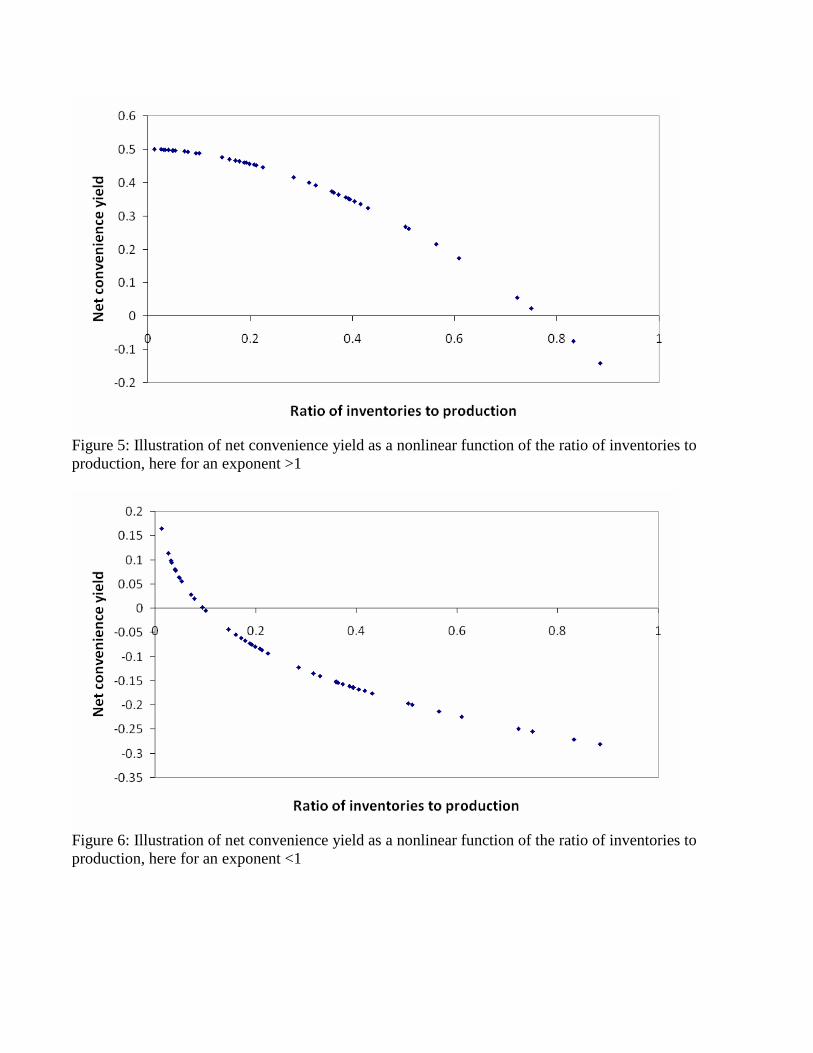
Figure 5: Illustration of net convenience yield as a nonlinear function of the ratio of inventories to production, here for an exponent >1

Figure 6: Illustration of net convenience yield as a nonlinear function of the ratio of inventories to production, here for an exponent <1