On Range Searching with Semialgebraic Sets II∗

PANKAJ K. AGARWALDepartment of Computer Science

Duke UniversityP.O. Box 90129

Durham, NC 27708-0129, USA

JIRI MATOUSEKDepartment of Applied Mathematics

Charles University, Malostranske nam. 25118 00 Praha 1, Czech Republic, and

Institute of Theoretical Computer ScienceETH Zurich, 8092 Zurich, Switzerland

MICHA SHARIRSchool of Computer Science,

Tel Aviv University,Tel Aviv 69978, Israel, and

Courant Institute of Mathematical Sciences,New York University,

New York, NY 10012, USA

May 30, 2013

Abstract

Let P be a set of n points in Rd. We present a linear-size data structure for answeringrange queries on P with constant-complexity semialgebraic sets as ranges, in time close toO(n1−1/d). It essentially matches the performance of similar structures for simplex rangesearching, and, for d ≥ 5, significantly improves earlier solutions by the first two authorsobtained in 1994. This almost settles a long-standing open problem in range searching.

The data structure is based on the polynomial-partitioning technique of Guth and Katz[arXiv:1011.4105], which shows that for a parameter r, 1 < r ≤ n, there exists a d-variatepolynomial f of degree O(r1/d) such that each connected component of Rd \ Z(f) containsat most n/r points of P , where Z(f) is the zero set of f . We present an efficient randomizedalgorithm for computing such a polynomial partition, which is of independent interest and islikely to have additional applications.

∗Work by Pankaj Agarwal was supported by NSF under grants IIS-07-13498, CCF-09-40671, CCF-10-12254, andCCF-11-61359, by ARO grants W911NF-07-1-0376 and W911NF-08-1-0452, and by an ARL award W9132V-11-C-0003. Work by Jirı Matousek has been supported by the ERC Advanced Grant No. 267165. Work by Micha Sharirhas been supported by NSF Grant CCF-08-30272, by Grant 338/09 from the Israel Science Fund, by the Israeli Centersfor Research Excellence (I-CORE) program (Center No. 4/11) and by the Hermann Minkowski–MINERVA Center forGeometry at Tel Aviv University. Part of the work was done while the first and third authors were visiting ETH Zurich.A preliminary version of the paper appeared in Proceedings of the 53rd Annual IEEE Symposium on Foundations ofComputer Science, 2012.

1

1 Introduction

Range searching. Let P be a set of n points in Rd, where d is a small constant. Let Γ be a familyof geometric “regions,” called ranges, in Rd, each of which can be described algebraically by somefixed number of real parameters (a more precise definition is given below). For example, Γ can bethe set of all axis-parallel boxes, balls, simplices, or cylinders, or the set of all intersections of pairsof ellipsoids. In the Γ-range searching problem, we want to preprocess P into a data structure sothat the number of points of P lying in a query range γ ∈ Γ can be counted efficiently. Similar tomany previous papers, we actually consider a more general setting, the so-called semigroup model,where we are given a weight function on the points in P and we ask for the cumulative weight ofthe points in P ∩ γ. The weights are assumed to belong to a semigroup, i.e., subtractions are notallowed. We assume that the semigroup operation can be executed in constant time.

In this paper we consider the case in which Γ is a set of constant-complexity semialgebraicsets. We recall that a semialgebraic set is a subset of Rd obtained from a finite number of sets ofthe form x ∈ Rd | g(x) ≥ 0, where g is a d-variate polynomial with integer coefficients,1 byBoolean operations (unions, intersections, and complementations). Specifically, let Γd,∆,s denotethe family of all semialgebraic sets in Rd defined by at most s polynomial inequalities of degreeat most ∆ each. If d,∆, s are all regarded as constants, we refer to the sets in Γd,∆,s as constant-complexity semialgebraic sets (such sets are sometimes also called Tarski cells). By semialgebraicrange searching we mean Γd,∆,s-range searching for some parameters d,∆, s; in most applicationsthe actual collection Γ of ranges is only a restricted subset of some Γd,∆,s. Besides being interestingin its own right, semialgebraic range searching also arises in several geometric searching problems,such as searching for a point nearest to a query geometric object, counting the number of inputobjects intersecting a query object, and many others.

This paper focuses on the low storage version of range searching with constant-complexitysemialgebraic sets—the data structure is allowed to use only linear or near-linear storage, and thegoal is to make the query time as small as possible. At the other end of the spectrum we have thefast query version, where we want queries to be answered in polylogarithmic time using as littlestorage as possible. This variant is discussed briefly in Section 8.

As is typical in computational geometry, we will use the real RAM model of computation, wherewe can compute exactly with arbitrary real numbers and each arithmetic operation is executed inconstant time.

Previous work. Motivated by a wide range of applications, several variants of range searchinghave been studied in computational geometry and database systems at least since the 1980s. See[1,23] for comprehensive surveys of this topic. The early work focused on the so-called orthogonalrange searching, where ranges are axis-parallel boxes. After three decades of extensive work onthis particular case, some basic questions still remain open. However, geometry plays little role inthe known data structures for orthogonal range searching.

The most basic and most studied truly geometric instance of range searching is with halfspaces,or more generally simplices, as ranges. Studies in the early 1990s have essentially determinedthe optimal trade-off between the worst-case query time and the storage (and preprocessing time)

1The usual definition of a semialgebraic set requires these polynomials to have integer coefficients. However, for ourpurposes, since we are going to assume the real RAM model of computation, we can actually allow for arbitrary realcoefficients without affecting the asymptotic overhead.

1

required by any data structure for simplex range searching.2 Lower bounds for this trade-off havebeen given by Chazelle [7] under the semigroup model of computation, where subtraction of thepoint weights is not allowed. It is possible that, say, the counting version of the simplex rangesearching problem, where we ask just for the number of points in the query simplex, might admitbetter solutions using subtractions, but no such solutions are known. Moreover, there are recentlower-bound results when subtractions are also allowed; see [19] and references therein.

The data structures proposed for simplex range searching over the last two decades [21, 22]match the known lower bounds within polylogarithmic factors. The state-of-the-art upper boundsare by (i) Chan [6], who, building on many earlier results, provides a linear-size data structurewith O(n log n) expected preprocessing time and O(n1−1/d) query time, and (ii) Matousek [22],who provides a data structure with O(nd) storage, O((log n)d+1) query time, and O(nd(log n)ε)preprocessing time.3 A trade-off between space and query time can be obtained by combining thesetwo data structures [22].

Yao and Yao [32] were perhaps the first to consider range searching in which ranges weredelimited by graphs of polynomial functions. Agarwal and Matousek [2] have introduced a sys-tematic study of semialgebraic range searching. Building on the techniques developed for simplexrange searching, they presented a linear-size data structure with O(n1−1/b+ε) query time, whereb = max(d, 2d− 4). For d ≤ 4, this almost matches the performance for the simplex range search-ing, but for d ≥ 5 there is a gap in the exponents of the corresponding bounds. Also see [28] forrelated recent developments.

The bottleneck in the performance of the just mentioned range-searching data structure of [2]is a combinatorial geometry problem, known as the decomposition of arrangements into constant-complexity cells. Here, we are given a set Σ of t algebraic surfaces in Rd (i.e., zero sets of d-variate polynomials), with degrees bounded by a constant ∆0, and we want to decompose eachcell of the arrangement A(Σ) (see Section 4 for details) into subcells that are constant-complexitysemialgebraic sets, i.e., belong to Γd,∆,s for some constants ∆ (bound on degrees) and s (numberof defining polynomials), which may depend on d and ∆0, but not on t. The crucial quantity is thetotal number of the resulting subcells over all cells of A(Σ); namely, if one can construct such adecomposition with O(tb) subcells, with some constant b, for every t and Σ, then the method of [2]yields query timeO(n1−1/b+ε) (with linear storage). The only known general-purpose technique forproducing such a decomposition is the so-called vertical decomposition [8, 27], which decomposesA(Σ) into roughly t2d−4 constant-complexity subcells, for d ≥ 4 [18, 27].

An alternative approach, based on linearization, was also proposed in [2]. It maps the semialge-braic ranges in Rd to simplices in some higher-dimensional space and uses simplex range searchingthere. However, its performance depends on the specific form of the polynomials defining theranges. In some special cases (e.g., when ranges are balls in Rd), linearization yields better querytime than the decomposition-based technique mentioned above, but for general constant-complexitysemialgebraic ranges, linearization has worse performance.

2This applies when d is assumed to be fixed and the implicit constants in the asymptotic notation may depend ond. This is the setting in all the previous papers, including the present one. Of course, in practical applications, thisassumption may be unrealistic unless the dimension is really small. However, the known lower bounds imply that if thedimension is large, no efficient solutions to simplex range searching exist, at least in the worst-case setting.

3Here and in the sequel, ε denotes an arbitrarily small positive constant. The implicit constants in the asymptoticnotation may depend on it, generally tending to infinity as ε decreases to 0.

2

Our results. In a recent breakthrough, Guth and Katz [12] have presented a new space de-composition technique, called polynomial partitioning. For a set P ⊂ Rd of n points and a realparameter r, 1 < r ≤ n, an r-partitioning polynomial for P is a nonzero d-variate polynomialf such that each connected component of Rd \ Z(f) contains at most n/r points of P , whereZ(f) := x ∈ Rd | f(x) = 0 denotes the zero set of f . The decomposition of Rd into Z(f) andthe connected components of Rd \ Z(f) is called a polynomial partition (induced by f ). Guth andKatz show that an r-partitioning polynomial of degree O(r1/d) always exists, but their argumentdoes not lead to an efficient algorithm for constructing such a polynomial, mainly because it relieson ham-sandwich cuts in high-dimensional spaces, for which no efficient construction is known.Our first result is an efficient randomized algorithm for computing an r-partitioning polynomial.

Theorem 1.1. Given a set P of n points in Rd, for some fixed d, and a parameter r ≤ n, anr-partitioning polynomial for P of degree O(r1/d) can be computed in randomized expected timeO(nr + r3).

Next, we use this algorithm to bypass the arrangement-decomposition problem mentioned above.Namely, based on polynomial partitions, we construct partition trees [1, 23] that answer rangequeries with constant-complexity semialgebraic sets in near-optimal time, using linear storage. Anessential ingredient in the performance analysis of these partition trees is a recent combinatorialresult of Barone and Basu [3], originally conjectured by the second author, which deals with thecomplexity of certain kinds of arrangements of zero sets of polynomials (see Theorem 4.2). Whilethere have already been several combinatorial applications of the Guth-Katz technique (the mostimpressive being the original one in [12], which solves the famous Erdos’s distinct distances prob-lem, and some of the others presented in [14, 15, 29, 34]), ours seems to be the first algorithmicapplication.

We establish two range-searching results, both based on polynomial partitions. For the firstresult, we need to introduce the notion of D-general position, for an integer D ≥ 1. We say that aset P ⊂ Rd is in D-general position if no k points of P are contained in the zero set of a nonzerod-variate polynomial of degree at most D, where k :=

(D+dd

). This is the number one expects for a

“generic” point set.4

Theorem 1.2. Let d,∆, s and ε > 0 be constants. Let P ⊂ Rd be an n-point set in D0-generalposition, where D0 is a suitable constant depending on d,∆, and ε. Then the Γd,∆,s-range search-ing problem for P can be solved with O(n) storage, O(n log n) expected preprocessing time, andO(n1−1/d+ε) query time.

We note that both here and in the next theorem, while the preprocessing algorithm is random-ized, the queries are answered deterministically, and the query time bound is worst-case.

Of course, we would like to handle arbitrary point sets, not only those in D0-general position.This can be achieved by an infinitesimal perturbation of the points of P . A general technique knownas “simulation of simplicity” (in the version considered by Yap [33]) ensures that the perturbed set

4Indeed, d-variate polynomials of degree at most D have at most k−1 distinct nonconstant monomials. The Veronesemap (e.g., see [12]) maps Rd to Rk−1, and hyperplanes in Rk−1 correspond bijectively to k-variate polynomials of degreeat most D. It follows that any set of k − 1 points in Rd is contained in the zero set of a d-variate polynomial of degreeat most D, corresponding to the hyperplane in Rk−1 passing through the Veronese images of these points. Similarly,k points in general position are not expected to have this property, because one does not expect their images to lie in acommon hyperplane. See [10, 11] for more details.

3

P ′ is in D0-general position. If a point p ∈ P lies in the interior of a query range γ, then so doesthe corresponding perturbed point p′ ∈ P ′, and similarly for p in the interior of Rd \ γ. However,for p on the boundary of γ, we cannot be sure if p′ ends up inside or outside γ.

Let us say that a boundary-fuzzy solution to the Γd,∆,s-range searching problem is a data struc-ture that, given a query γ ∈ Γd,∆,s, returns an answer in which all points of P in the interior of γ arecounted and none in the interior of Rd \ γ is counted, while each point p ∈ P on the boundary of γmay or may not be counted. In some applications, we can think of the points of P being impreciseanyway (e.g., their coordinates come from some imprecise measurement), and then boundary-fuzzyrange searching may be adequate.

Corollary 1.3. Let d,∆, s, and ε > 0 be constants. Then for every n-point set in Rd, there isa boundary-fuzzy Γd,∆,s-range searching data structure with O(n) storage, O(n log n) expectedpreprocessing time, and O(n1−1/d+ε) query time.

Actually, previous results on range searching that use simulation of simplicity to avoid degen-erate cases also solve only the boundary-fuzzy variant (see e.g. [21, 22]). However, the previoustechniques, even if presented only for point sets in general position, can usually be adapted tohandle degenerate cases as well, perhaps with some effort, which is nevertheless routine. For ourtechnique, degeneracy appears to be a more substantial problem because it is possible that a largesubset of P (maybe even all of P ) is contained in the zero set of the partitioning polynomial f ,and the recursive divide-and-conquer mechanism yielded by the partition of f does not apply to thissubset.

Partially in response to this issue, we present a different data structure that, at a somewhat higherpreprocessing cost, not only gets rid of the boundary-fuzziness condition but also has a slightlyimproved query time (in terms of n). The main idea is that we build an auxiliary recursive datastructure to handle the potentially large subset of points that lie in the zero set of the partitioningpolynomial.

Theorem 1.4. Let d,∆, s, and ε > 0 be constants. Then the Γd,∆,s-range searching problem for anarbitrary n-point set in Rd can be solved with O(n) storage, O(n1+ε) expected preprocessing time,and O(n1−1/d logB n) query time, where B is a constant depending on d,∆, s and ε.

We remark that the dependence of B on ∆, s, and ε is reasonable, but its dependence on d issuperexponential.

Our algorithms work for the semigroup model described earlier. Assuming that a semigroupoperation can be executed in constant time, the query time remains the same as for the countingquery. A reporting query—report the points of P lying in a query range—also fits in the semigroupmodel, except one cannot assume that a semigroup operation in this case takes constant time. Thetime taken by a reporting query is proportional to the cost of a counting query plus the number ofreported points.

Roadmap of the paper. Our algorithm is based on the polynomial partitioning technique by Guthand Katz, and we begin by briefly reviewing it in Section 2. Next, in Section 3, we describe the ran-domized algorithm for constructing such a partitioning polynomial. Section 4 presents an algorithmfor computing the cells of a polynomial partition that are crossed by a semialgebraic range, and dis-cusses several related topics. Section 5 presents our first data structure, which is as in Theorem 1.2.

4

Section 6 describes the method for handling points lying on the zero set of the partitioning polyno-mial, and Section 7 presents our second data structure. We conclude in Section 8 by mentioning afew open problems.

2 Polynomial Partitions

In this section we briefly review the Guth-Katz technique for later use. We begin by stating theirresult.

Theorem 2.1 (Guth-Katz [12]). Given a set P of n points in Rd and a parameter r ≤ n, there existsan r-partitioning polynomial for P of degree at most O(r1/d) (for d fixed).

The degree in the theorem is asymptotically optimal in the worst case because the number ofconnected components of Rd \ Z(f) is O((deg f)d) for every polynomial f (see, e.g., Warren [31,Theorem 2]).

Sketch of proof. The Guth-Katz proof uses the polynomial ham sandwich theorem of Stone andTukey [30], which we state here in a version for finite point sets: If A1, . . . , Ak are finite sets in Rdand D is an integer satisfying

(D+dd

)− 1 ≥ k, then there exists a nonzero polynomial f of degree at

most D that simultaneously bisects all the sets Ai. Here “f bisects Ai” means that f > 0 in at mostb|Ai|/2c points of Ai and f < 0 in at most b|Ai|/2c points of Ai; f might vanish at any number ofthe points of Ai, possibly even at all of them.

Guth and Katz inductively construct collections P0,P1, . . . ,Pm of subsets of P . For j =0, 1, . . . ,m, Pj consists of at most 2j pairwise-disjoint subsets of P , each of size at most n/2j ;the union of these sets does not have to contain all points of P .

Initially, we have P0 = P. The algorithm stops as soon as each subset in Pm has at mostn/r points. This implies that m ≤ dlog2 re. Having constructed Pj−1, we use the polynomialham-sandwich theorem to construct a polynomial fj that bisects each set of Pj−1, with deg fj =

O(2j/d) (this is indeed an asymptotic upper bound for the smallest D satisfying(D+dd

)− 1 ≥ 2j−1,

assuming d to be a constant). For every subset Q ∈ Pj−1, let Q+ = q ∈ Q | fj(q) > 0 andQ− = q ∈ Q | fj(q) < 0. We set Pj := Q+, Q− | Q ∈ Pj−1; empty subsets are not includedin Pj .

The desired r-partitioning polynomial for P is then the product f := f1f2 · · · fm. We have

deg f =m∑j=1

deg fj =m∑j=1

O(2j/d) = O(r1/d).

By construction, the points of P lying in a single connected component of Rd \ Z(f) belong to asingle member of Pm, which implies that each connected component contains at most n/r pointsof P .

Sketch of proof of the Stone–Tukey polynomial ham-sandwich theorem. We begin by observingthat

(D+dd

)− 1 is the number of all nonconstant monomials of degree at most D in d variables.

Thus, we fix a collection M of k ≤(D+dd

)− 1 such monomials. Let Φ: Rd → Rk be the corre-

sponding Veronese map, which maps a point x = (x1, . . . , xd) ∈ Rd to the k-tuple of the values at(x1, . . . , xd) of the monomials from M. For example, for d = 2, D = 3, and k = 8 ≤

(3+2

2

)− 1,

5

we may use Φ(x1, x2) = (x1, x2, x21, x1x2, x

22, x

31, x

21x2, x1x

22) ∈ R8, where M is the set of the

eight monomials appearing as components of Φ.Let Bi := Φ(Ai) ⊂ Rk be the image of the given Ai under this Veronese map, for i = 1, . . . , k.

By the standard ham-sandwich theorem (see, e.g., [24]), there exists a hyperplane h in Rk thatsimultaneously bisects all the Bi’s, in the sense that each open halfspace bounded by h containsat most half of the points of each of the sets Bi. In a more algebraic language, there is a nonzerok-variate linear polynomial, which we also call h, that bisects all the Bi’s, in the sense of beingpositive on at most half of the points of each Bi, and being negative on at most half of the pointsof each Bi. Then f := h Φ is the desired d-variate polynomial of degree at most D bisecting allthe Ai’s.

3 Constructing a Partitioning Polynomial

In this section we present an efficient randomized algorithm that, given a point set P and a parameterr < n, constructs an r-partitioning polynomial. The main difficulty in converting the above proofof the Guth-Katz partitioning theorem into an efficient algorithm is the use of the ham-sandwichtheorem in the possibly high-dimensional space Rk. A straightforward algorithm for computingham-sandwich cuts in Rk inspects all possible ways of splitting the input point sets by a hyperplane,and has running time about nk. Compared to this easy upper bound, the best known ham-sandwichalgorithms can save a factor of about n [20], but this is insignificant in higher dimensions. A recentresult of Knauer, Tiwari, and Werner [17] shows that a certain incremental variant of computinga ham-sandwich cut is W [1]-hard (where the parameter is the dimension), and thus one perhapsshould not expect much better exact algorithms.

We observe that the exact bisection of each Ai is not needed in the Guth-Katz construction—itis sufficient to replace the Stone–Tukey polynomial ham-sandwich theorem by a weaker result, asdescribed below.

Constructing a well-dissecting polynomial. We say that a polynomial f is well-dissecting for apoint setA if f > 0 on at most 7

8 |A| points ofA and f < 0 on at most 78 |A| points ofA. Given point

sets A1, . . . , Ak in Rd with n points in total, we present a Las-Vegas algorithm for constructing apolynomial f of degree O(k1/d) that is well-dissecting for at least dk/2e of the Ai’s.

As in the above proof of the Stone–Tukey polynomial ham-sandwich theorem, let D be thesmallest integer satisfying

(D+dd

)− 1 ≥ k. We fix a collection M of k distinct nonconstant mono-

mials of degree at most D, and let Φ be the corresponding Veronese map. For each i = 1, 2, . . . , k,we pick a point ai ∈ Ai uniformly at random and compute bi := Φ(ai). Let h be a hyperplane in Rkpassing through b1, . . . , bk, which can be found by solving a system of linear equations, in O(k3)time.

If the points b1, . . . , bk are not affinely independent, then h is not determined uniquely (thisis a technical nuisance, which the reader may want to ignore on first reading). In order to handlethis case, we prepare in advance, before picking the ai’s, auxiliary affinely independent pointsq1, . . . , qk in Rk, which are in general position with respect to Φ(A1), . . . ,Φ(Ak); here we meanthe “ordinary” general position, i.e., no unnecessary affine dependences, that involve some of theqi’s and the other points, arise. The points qi can be chosen at random, say, uniformly in the unitcube; with high probability, they have the desired general position property. (If we do not want

6

to assume the capability of choosing a random real number, we can pick the qi’s uniformly atrandom from a sufficiently large discrete set.) If the dimension of the affine hull of b1, . . . , bk isk′ < k − 1, we choose the hyperplane h through b1, . . . , bk and q1, . . . , qk−k′−1. If h is not unique,i.e., q1, . . . qk−k′−1 are not affinely independent with respect to b1, . . . bk, which we can detect whilesolving the linear system, we restart the algorithm by choosing q1, . . . , qk anew and then pickingnew a1, . . . , ak. In this way, after a constant expected number of iterations, we obtain the uniquelydetermined hyperplane h through b1, . . . , bk and q1, . . . , qk−k′−1 as above, and we let f = h Φdenote the corresponding d-variate polynomial. We refer to these steps as one trial of the algorithm.For each Ai, we check whether f is well-dissecting for Ai. If f is well-dissecting for only fewerthan k/2 sets, then we discard f and perform another trial.

We now analyze the expected running time of the algorithm. The intuition is that f is expectedto well-dissect a significant fraction, say at least half, of the sets Ai. This intuition is reflected in thenext lemma. Let Xi be the indicator variable of the event: Ai is not well-dissected by f .

Lemma 3.1. For every i = 1, 2, . . . , k, E[Xi] ≤ 1/4.

Proof. Let us fix i and the choices of aj (and thus of bj = Φ(aj)) for all j 6= i. Let k0 be thedimension of F0, the affine hull of bj | j 6= i. Then the resulting hyperplane h passes through the(k−2)-flat F spanned by F0 and q1, . . . , qk−k0−2, irrespective of which point ofAi is chosen. If ai,the point chosen from Ai, is such that bi = Φ(ai) lies on F0, then h also passes through qk−k0−1.

Put Bi := Φ(Ai), and let us project the configuration orthogonally to a 2-dimensional planeπ orthogonal to F . Then F appears as a point F ∗ ∈ π, and Bi projects to a (multi)set B∗i in π.The random hyperplane h projects to a random line h∗ in π, whose choice can be interpreted asfollows: pick b∗i ∈ B∗i uniformly at random; if b∗i 6= F ∗, then h∗ is the unique line through b∗iand F ∗; otherwise, when b∗i = F ∗, h∗ is the unique line through F ∗ and q∗k−k0−1; by construction,q∗k−k0−1 6= F ∗. The indicator variable Xi is 1 if and only if the resulting h∗ has more than 7

8 |B∗i |points of B∗i , counted with multiplicity, (strictly) on one side.

The special role of q∗k−k0−1 can be eliminated if we first move the points of B∗i coinciding withF ∗ to the point q∗k−k0−1, and then slightly perturb the points so as to ensure that all points of B∗iare distinct and lie at distinct directions from F ∗; it is easy to see that these transformations cannotdecrease the probability of Xi = 1. Finally, we note that the side of h∗ containing a point b∗ ∈ B∗ionly depends on the direction of the vector

−−→F ∗b∗, so we can also assume the points of B∗i to lie on

the unit circle around F ∗.Using (a simple instance of) the standard planar ham-sandwich theorem, we partition B∗i into

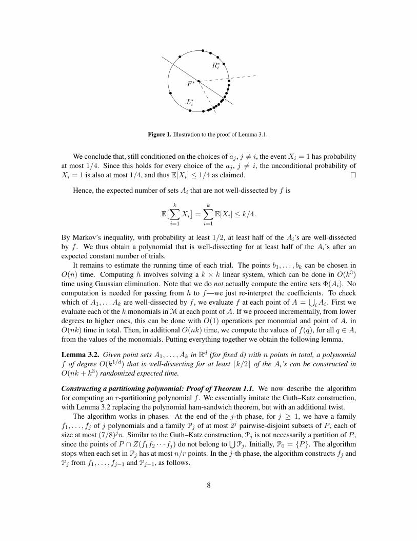
two subsets L∗i and R∗i of equal size by a line through the center F ∗. Then we bisect L∗i by a rayfrom F ∗, and we do the same for R∗i . It is easily checked (see Figure 1) that there always existtwo of the resulting quarters, one of L∗i and one of R∗i (the ones whose union forms an angle ≤ πbetween the two bisecting rays), such that every line connecting F ∗ with a point in either quartercontains at least 1

4 |B∗i | points of B∗i on each side. Referring to these quarters as “good”, we nowtake one of the bisecting rays, say that of L∗i , and rotate it about F ∗ away from the good quarter ofL∗i . Each of the first 1

8 |B∗i | points that the ray encounters has the property that the line supporting theray has at least 1

8 |B∗i | points of B∗i on each side. This implies that, for at least half of the points ineach of the two remaining quarters, the line connecting F ∗ to such a point has at least 1

8 |B∗i | pointsof B∗i on each side. Hence at most 1

4 |Bi| points of Bi can lead to a cut that is not well-dissectingfor Bi.

7

L∗i

R∗i

F ∗

Figure 1. Illustration to the proof of Lemma 3.1.

We conclude that, still conditioned on the choices of aj , j 6= i, the event Xi = 1 has probabilityat most 1/4. Since this holds for every choice of the aj , j 6= i, the unconditional probability ofXi = 1 is also at most 1/4, and thus E[Xi] ≤ 1/4 as claimed.

Hence, the expected number of sets Ai that are not well-dissected by f is

E[ k∑i=1

Xi

]=

k∑i=1

E[Xi] ≤ k/4.

By Markov’s inequality, with probability at least 1/2, at least half of the Ai’s are well-dissectedby f . We thus obtain a polynomial that is well-dissecting for at least half of the Ai’s after anexpected constant number of trials.

It remains to estimate the running time of each trial. The points b1, . . . , bk can be chosen inO(n) time. Computing h involves solving a k × k linear system, which can be done in O(k3)time using Gaussian elimination. Note that we do not actually compute the entire sets Φ(Ai). Nocomputation is needed for passing from h to f—we just re-interpret the coefficients. To checkwhich of A1, . . . Ak are well-dissected by f , we evaluate f at each point of A =

⋃iAi. First we

evaluate each of the k monomials in M at each point of A. If we proceed incrementally, from lowerdegrees to higher ones, this can be done with O(1) operations per monomial and point of A, inO(nk) time in total. Then, in additional O(nk) time, we compute the values of f(q), for all q ∈ A,from the values of the monomials. Putting everything together we obtain the following lemma.

Lemma 3.2. Given point sets A1, . . . , Ak in Rd (for fixed d) with n points in total, a polynomialf of degree O(k1/d) that is well-dissecting for at least dk/2e of the Ai’s can be constructed inO(nk + k3) randomized expected time.

Constructing a partitioning polynomial: Proof of Theorem 1.1. We now describe the algorithmfor computing an r-partitioning polynomial f . We essentially imitate the Guth–Katz construction,with Lemma 3.2 replacing the polynomial ham-sandwich theorem, but with an additional twist.

The algorithm works in phases. At the end of the j-th phase, for j ≥ 1, we have a familyf1, . . . , fj of j polynomials and a family Pj of at most 2j pairwise-disjoint subsets of P , each ofsize at most (7/8)jn. Similar to the Guth–Katz construction, Pj is not necessarily a partition of P ,since the points of P ∩ Z(f1f2 · · · fj) do not belong to

⋃Pj . Initially, P0 = P. The algorithm

stops when each set in Pj has at most n/r points. In the j-th phase, the algorithm constructs fj andPj from f1, . . . , fj−1 and Pj−1, as follows.

8

At the beginning of the j-th phase, let Lj = Q ∈ Pj−1 | |Q| > (7/8)jn be the familyof the “large” sets in Pj−1, and set κj = |Lj | ≤ (8/7)j . We also initialize the collection Pj toPj−1 \ Lj , the family of “small” sets in Pj−1. Then we perform at most dlog2 κje dissecting steps,as follows: After s steps, we have a family g1, . . . , gs of polynomials, the current set Pj , and asubfamily L

(s)j ⊆ Lj of size at most κj/2s, consisting of the members of Lj that were not well-

dissected by any of g1, . . . , gs. If L(s)j 6= ∅ we choose, using Lemma 3.2, a polynomial gs+1 of

degree at most c(κj/2s)1/d (with a suitable constant c that depends only on d) that well-dissectsat least half of the members of L

(s)j . For each Q ∈ L

(s)j , let Q+ = q ∈ Q | gs+1(q) > 0

and Q− = q ∈ Q | gs+1(q) < 0. If Q is well-dissected, i.e., |Q+|, |Q−| ≤ 78 |Q|, then we

add Q+, Q− to Pj , and otherwise, we add Q to L(s+1)j . Note that in the former case the points

q ∈ Q satisfying gs+1(q) = 0 are “lost” and do not participate in the subsequent dissections. ByLemma 3.2, |L(s+1)

j | ≤ |L(s)j |/2 ≤ κj/2s+1.

The j-th phase is completed when L(s)j = ∅, in which case we set5 fj :=

∏s`=1 g`. By construc-

tion, each point set in Pj has at most (7/8)jn points, and the points of P not belonging to any setof Pj lie in Z(f1 · · · fj). Furthermore,

deg fj ≤∑s≥0

c(κj/2s)1/d = O(κ

1/dj ),

where again the constant of proportionality depends only on d. Since every set in Pj−1 is split intoat most two sets before being added to Pj , |Pj | ≤ 2|Pj−1| ≤ 2j .

If Pj contains subsets with more than n/r points, we begin the (j+ 1)-st phase with the currentPj ; otherwise the algorithm stops and returns f := f1f2 · · · fj . This completes the description ofthe algorithm.

Clearly, m, the number of phases of the algorithm, is at most dlog8/7 re. Following the sameargument as in [12], and as briefly sketched in Section 2, it can be shown that all points lying in asingle connected component of Rd\Z(f) belong to a single member of Pm, and thus each connectedcomponent contains at most n/r points of P . Since the degree of fj is O(κ

1/dj ), κj ≤ (8/7)j , and

m ≤ dlog8/7 re, we conclude that

deg f = O

( m∑j=1

κ1/dj

)= O

( m∑j=1

(8/7)j/d)

= O(r1/d).

As for the expected running time of the algorithm, the s-th step of the j-th phase takesO(nκj/2s+

(κj/2s)3) expected time, so the j-th phase takes a total of O(nκj +κ3

j ) expected time. Substitutingκj ≤ (8/7)j in the above bound and summing over all j, the overall expected running time of thealgorithm is O(nr + r3). This completes the proof of Theorem 1.1.

Remark. Theorem 1.1 is employed for the preprocessing in our range-searching algorithms inTheorems 1.2 and 1.4. In Theorem 1.2 we take r to be a large constant, and the expected runningtime in Theorem 1.1 is O(n). However, in Theorem 1.4, we require r to be a small fractional power

5Note that fj is not necessarily well-dissecting, because it does not control the sizes of subsets with positive or withnegative signs.

9

of n, say r = n0.001. It is a challenging open problem to improve the expected running time inTheorem 1.1 to O(n polylog(n)) when r is such a small fractional power of n. The bottleneckin the current algorithm is the subproblem of evaluating a given d-variate polynomial f of degreeD = O(r1/d) at n given points; everything else can be performed in O(n polylog(r) + rO(1))expected time. Finding the signs of f at those points would actually suffice, but this probably doesnot make the problem any simpler.

This problem of multi-evaluation of multivariate real polynomials has been considered in theliterature, and there is a nontrivial improvement over the straightforward O(nr) algorithm, due toNusken and Ziegler [25]. Concretely, in the bivariate case (d = 2), their algorithm can evaluate abivariate polynomial of degree D ≤ √n at n given points using O(nD0.667) arithmetic operations.It is based on fast matrix multiplication, and even under the most optimistic possible assumption onthe speed of matrix multiplication, it cannot get below nD1/2. Although this is significantly fasterthan our naiveO(nr)-time algorithm, which isO(nD2) in this bivariate case, it is still a far cry fromwhat we are aiming at. Let us remark that in a different setting, for polynomials over finite fields(and over certain more general finite rings), there is a remarkable method for multi-evaluation byKedlaya and Umans [16] achievingO(((n+Dd) log q)1+ε) running time, where q is the cardinalityof the field.

4 Crossing a Polynomial Partition with a Range

In this section we define the crossing number of a polynomial partition and describe an algorithmfor computing the cells of a polynomial partition that are crossed by a semialgebraic range, both ofwhich will be crucial for our range-searching data structures. We begin by recalling a few results onarrangements of algebraic surfaces. We refer the reader to [27] for a comprehensive review of sucharrangements.

Let Σ be a finite set of algebraic surfaces in Rd. The arrangement of Σ, denoted by A(Σ), isthe partition of Rd into maximal relatively open connected subsets, called cells, such that all pointswithin each cell lie in the same subset of surfaces of Σ (and in no other surface). If F is a set ofd-variate polynomials, then with a slight abuse of notation, we use A(F) to denote the arrangementA(Z(f) | f ∈ F) of their zero sets. We need the following result on arrangements, which followsfrom Proposition 7.33 and Theorem 16.18 in [5].

Theorem 4.1 (Basu, Pollack and Roy [5]). Let F = f1, . . . , fs be a set of s real d-variate polyno-mials, each of degree at most ∆. Then the arrangement A(F) in Rd has at most O(1)d(s∆)d cells,and it can be computed in time at most T = sd+1∆O(d4). Each cell is described as a semialgebraicset using at most T polynomials of degree bounded by ∆O(d3). Moreover, the algorithm supplies anexplicitly computed point in each cell.

A key ingredient for the analysis of our range-searching data structure is the following recentresult of Barone and Basu [3], which is a refinement of a series of previous studies; e.g., see [4, 5]:

Theorem 4.2 (Barone and Basu [3]). Let V be a k-dimensional algebraic variety in Rd defined by afinite set G of d-variate polynomials, each of degree at most ∆, and let F be a set of s polynomials ofdegree at most D ≥ ∆. Then the number of cells of A(F∪G) (of all dimensions) that are containedin V is bounded by O(1)d∆d−k(sD)k.

10

The crossing number of polynomial partitions. Let P be a set of n points in Rd, and let fbe an r-partitioning polynomial for P . Recall that the polynomial partition Ω = Ω(f) inducedby f is the partition of Rd into the zero set Z(f) and the connected components ω1, ω2, . . . , ωt ofRd \ Z(f). As already noted, Warren’s theorem [31] implies that t = O(r). We call ω1, . . . , ωtthe cells of Ω (although they need not be cells in the sense typical, e.g., in topology; they need noteven be simply connected). Ω also induces a partition P ∗, P1, . . . , Pt of P , where P ∗ = P ∩ Z(f)is the exceptional part, and Pi = P ∩ ωi, for i = 1, . . . , t, are the regular parts. By construction,|Pi| ≤ n/r for every i = 1, 2, . . . , t, but we have no control over the size of P ∗—this will be thesource of most of our technical difficulties.

Next, let γ be a range in Γd,∆,s. We say that γ crosses a cell ωi if neither ωi ⊆ γ nor ωi∩γ = ∅.The crossing number of γ is the number of cells of Ω crossed by γ, and the crossing number of Ω(with respect to Γd,∆,s) is the maximum of the crossing numbers of all γ ∈ Γd,∆,s. Similar to manyprevious range-searching algorithms [6, 21, 22], the crossing number of Ω will determine the querytime of our range-searching algorithms described in Sections 5 and 7.

Lemma 4.3. If Ω is a polynomial partition induced by an r-partitioning polynomial of degree atmost D, then the crossing number of Ω with respect to Γd,∆,s, with ∆ ≤ D, is at most Cs∆Dd−1,where C is a suitable constant depending only on d.

Proof. Let γ ∈ Γd,∆,s; then γ is a Boolean combination of up to s sets of the form γj := x ∈ Rd |gj(x) ≥ 0, where g1, . . . , gs are polynomials of degree at most ∆. If γ crosses a cell ωi, then atleast one of the ranges γj also crosses ωi, and thus it suffices to establish that the crossing numberof any range γ, defined by a single d-variate polynomial inequality g(x) ≥ 0 of degree at most ∆,is at most C∆Dd−1.

We apply Theorem 4.2 with V := Z(g), which is an algebraic variety of dimension k ≤ d− 1,and with s = 1 and F = f, where f is the r-partitioning polynomial. Then, for each cell ωicrossed by γ, ωi ∩ Z(g) is a nonempty union of some of the cells in A(F ∪ g) = A(f, g) thatlie in V . Thus, the crossing number of γ is at most O(1)d∆Dd−1.

Algorithmic issues. We need to perform the following algorithmic primitives (for d fixed asusual) for the range-searching algorithms that we will later present:

(A1) Given an r-partitioning polynomial f of degree D = O(r1/d), compute (a suitable represen-tation of) the partition Ω and the induced partition of P into P ∗, P1, . . . , Pt.

By computing A(f), using Theorem 4.1, and then testing the membership of each pointp ∈ P in each cell ωi in time polynomial in r, the above operation can be performed inO(nrc) time,6 where c = dO(1).

(A2) Given (a suitable representation of) Ω as in (A1) and a query range γ ∈ Γd,∆,1, i.e., a rangedefined by a single d-variate polynomial g of degree ∆ ≤ D, compute which of the cells ofΩ are crossed by γ and which are completely contained in γ.

6Of course, this is somewhat inefficient, and it would be nice to have a fast point-location algorithm for the partitionΩ—this would be the second step, together with an improved construction of an r-partitioning polynomial f (concretely,an improved multi-point evaluation procedure for f ) as discussed at the end of Section 3, needed to improve the prepro-cessing time in Theorem 1.4.

11

We already have the arrangement A(f), and we compute A(f, g). For each cell ofA(f, g) contained in Z(g), we locate its representative point in A(f), and this gives usthe cells crossed by γ. For the remaining cells, we want to know whether they are inside γ oroutside, and for that, it suffices to determine the sign of g at the representative points. UsingTheorem 4.1, the above task can thus be accomplished in time O(rc), with c = dO(1).

5 Constant Fan-Out Partition Tree

We are now ready to describe our first data structure for Γd,∆,s-range searching, which is a constantfan-out (branching degree) partition tree, and which works for points in general position.

Proof of Theorem 1.2. Let P be a set of n points in Rd, and let ∆, s be constants. We choose ras a (large) constant depending on d,∆, s, and the prespecified parameter ε. We assume P to bein D0-general position for some sufficiently large constant D0 r1/d. We construct a partitiontree T of fan-out O(r) as follows. We first construct an r-partitioning polynomial f for P usingTheorem 1.1, and compute the partition Ω of Rd induced by f , as well as the corresponding partitionP = P ∗ ∪ P1 ∪ · · · ∪ Pt of P , where t = O(r). Since r is a constant, the (A1) operation, discussedin Section 4, performs this computation in O(n) time. We choose D0 so as to ensure that it isat least deg f , and then our assumption that P is in D0-general position implies that the size ofP ∗ = P ∩ Z(f) is bounded by D0.

We set up the root of T, where we store

(i) the partitioning polynomial f , and a suitable representation of the partition Ω;

(ii) a list of the points of the exceptional part P ∗; and

(iii) w(Pi), the sum of the weights of the points of the regular part Pi, for each i = 1, 2, . . . , t.

The regular parts Pi are not stored explicitly at the root. Instead, for each Pi we recursively builda subtree representing it. The recursion terminates, at leaves of T, as soon as we reach point setsof size smaller than a suitable constant n0. The points of each such set are stored explicitly at thecorresponding leaf of T.

Since each node of T requires only a constant amount of storage and each point of P is storedat only one node of T, the total size of T is O(n). The preprocessing time is O(n log n) since T hasdepth O(logr n) and each level is processed in O(n) time.

To process a query range γ ∈ Γd,∆,s, we start at the root of T and maintain a global counterwhich is initially set to 0. Among the cells ω1, . . . , ωt of the partition Ω stored at the root, we find,using the (A2) operation, those completely contained in γ, and those crossed by γ. Actually, wecompute a superset of the cells that γ crosses, namely, the cells crossed by the zero set of at leastone of the (at most s) polynomials defining γ. For each cell ωi ⊆ γ, we add the weight w(Pi) tothe global counter. We also add to the global counter the weights of the points in P ∗ ∩ γ, whichwe find by testing each point of P ∗ separately. Then we recurse in each subtree corresponding toa cell ωi crossed by γ (in the above weaker sense). The leaves, with point sets of size O(1), areprocessed by inspecting their points individually. By Lemma 4.3, the number of cells crossed byany of the polynomials defining γ at any interior node of T is at mostCs∆Dd−1 ≤ C ′r1−1/d, whereC ′ = C ′(d, s,∆) is a constant independent of r.

12

The query time Q(n) obeys the following recurrence:

Q(n) ≤C ′r1−1/dQ(n/r) +O(1) for n > n0,O(n) for n ≤ n0,

It is well known (e.g., see [21]), and easy to check, that the recurrence solves to Q(n) = O(n1−1/d+ε),for every fixed ε > 0, with an appropriate sufficiently large choice of r as a function of C ′ and ε,and with an appropriate choice of n0. This concludes the proof of Theorem 1.2.

Boundary-fuzzy range searching: Proof of Corollary 1.3. Now we consider the case where thepoints of P are not necessarily in D0-general position. As was mentioned in the introduction,we apply a general perturbation scheme of Yap [33] to the previous range-searching algorithm.

Yap’s scheme is applicable to an algorithm whose input is a sequence of real numbers (in ourcase, the dn point coordinates plus the coefficients in the polynomials specifying the query range). Itis assumed that the algorithm makes decision steps by way of evaluating polynomials with rationalcoefficients taken from a finite set P, where the input parameters are substituted for the variables.The algorithm makes a 3-way branching depending on the sign of the evaluation. The set P doesnot depend on the input. The input is considered degenerate if one of the signs in the tests is 0.

Yap’s scheme provides a black box for evaluating the polynomials from P that, whenever theactual value is 0, also supplies a nonzero sign, +1 or −1, which the algorithm may use for thebranching, instead of the zero sign. Thus, the algorithm never “sees” any degeneracy. Yap’s methodguarantees that these signs are consistent, i.e., for every input, the branching done in this waycorresponds to some infinitesimal perturbation of the input sequence, and so does the output of thealgorithm (in our case, the answer to a range-searching query).

For us, it is important that if the degrees of the polynomials in P are bounded by a constant,the black box also operates in time bounded by a constant (which is apparent from the explicitspecification in [33]). Thus, applying the perturbation scheme influences the running time only bya multiplicative constant.

It can be checked the range-searching algorithm presented above is of the required kind, withall branching steps based on the sign of suitable polynomials in the coordinates of the input pointsand in the coefficients of the polynomials in the query range, and the degrees of these polynomialsare bounded by a constant. For producing the partitioning polynomial f , we solve systems of linearequations, and thus the coefficients of f are given by certain determinants obtained from Cramer’srule. The computation of the polynomial partition and locating points in it is also based on the signsof suitable bounded-degree polynomials, as can be checked by inspecting the relevant algoritms,and similarly for intersecting a polynomial partition with the query range. The key fact is that allcomputations in the algorithm are of constant-bounded depth—each of the values ever computed isobtained from the input parameters by a constant number of arithmetic operations.

We also observe that when Yap’s scheme is applied, the algorithm never finds more than D0

points in the exceptional set P ∗ (in any of the nodes of the partition tree). Indeed, if D0 + 1 inputpoints lie in the zero set of a polynomial f as in the algorithm, then a certain polynomial in thecoordinates of these D0 + 1 points vanishes (see, e.g., [14, Lemma 6.3]). Thus, assuming that thealgorithm found D0 + 1 points on Z(f), it could test the sign of this polynomial at such points,and the black box would return a nonzero sign, which would contradict the consistency of Yap’sscheme.

13

Z(f)

H = xd = 0

π1

π2

π3

π4

π5

γ

γπ1

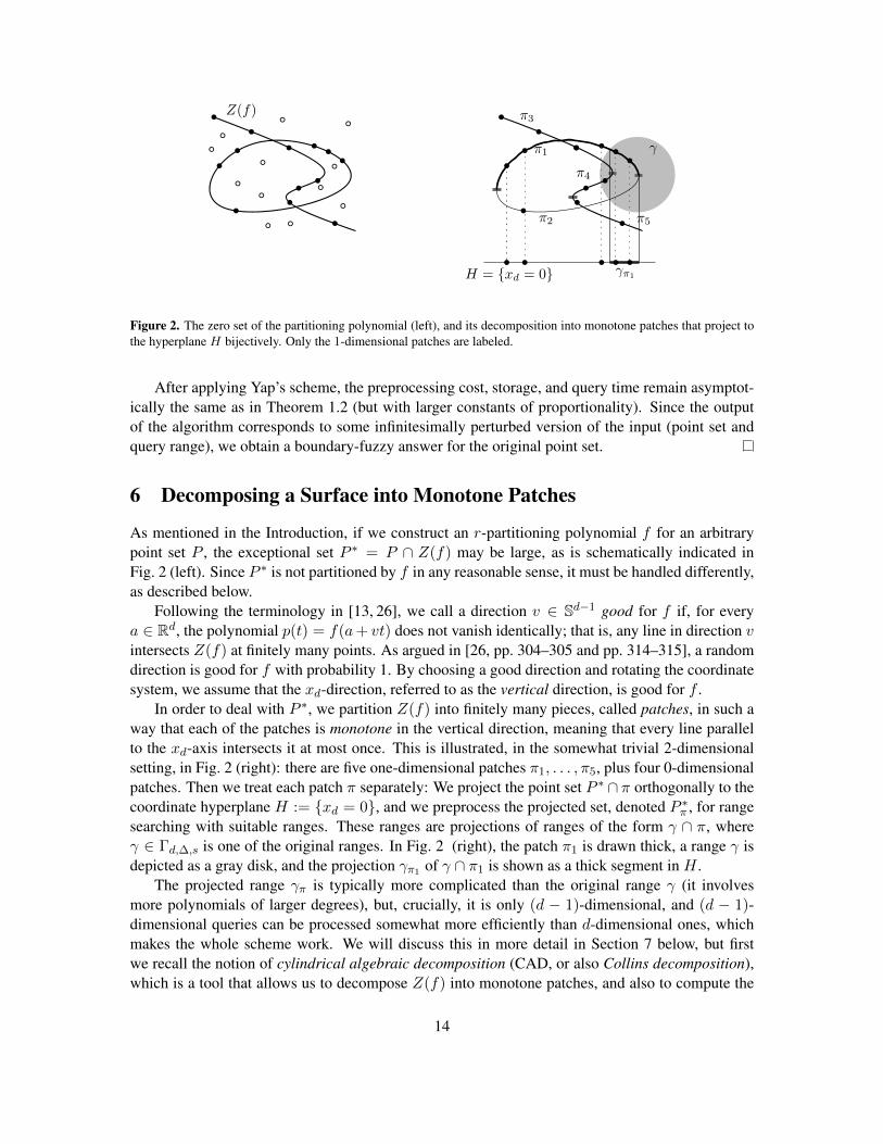
Figure 2. The zero set of the partitioning polynomial (left), and its decomposition into monotone patches that project tothe hyperplane H bijectively. Only the 1-dimensional patches are labeled.

After applying Yap’s scheme, the preprocessing cost, storage, and query time remain asymptot-ically the same as in Theorem 1.2 (but with larger constants of proportionality). Since the outputof the algorithm corresponds to some infinitesimally perturbed version of the input (point set andquery range), we obtain a boundary-fuzzy answer for the original point set.

6 Decomposing a Surface into Monotone Patches

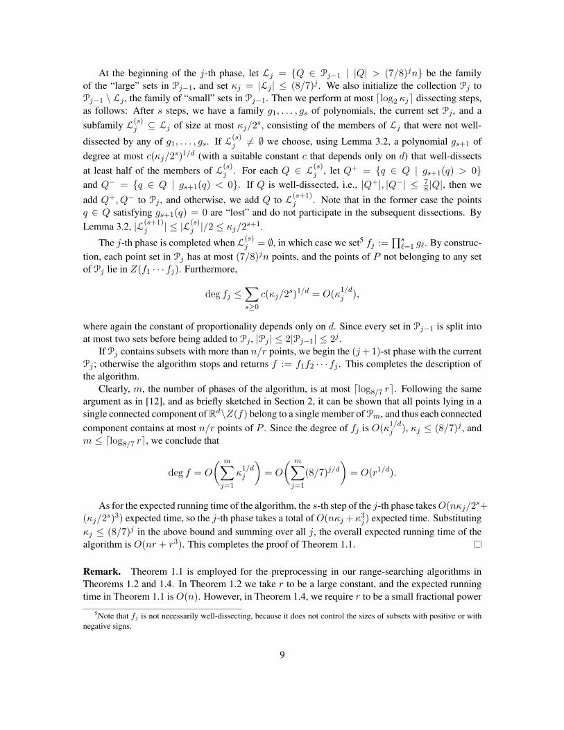
As mentioned in the Introduction, if we construct an r-partitioning polynomial f for an arbitrarypoint set P , the exceptional set P ∗ = P ∩ Z(f) may be large, as is schematically indicated inFig. 2 (left). Since P ∗ is not partitioned by f in any reasonable sense, it must be handled differently,as described below.

Following the terminology in [13, 26], we call a direction v ∈ Sd−1 good for f if, for everya ∈ Rd, the polynomial p(t) = f(a+ vt) does not vanish identically; that is, any line in direction vintersects Z(f) at finitely many points. As argued in [26, pp. 304–305 and pp. 314–315], a randomdirection is good for f with probability 1. By choosing a good direction and rotating the coordinatesystem, we assume that the xd-direction, referred to as the vertical direction, is good for f .

In order to deal with P ∗, we partition Z(f) into finitely many pieces, called patches, in such away that each of the patches is monotone in the vertical direction, meaning that every line parallelto the xd-axis intersects it at most once. This is illustrated, in the somewhat trivial 2-dimensionalsetting, in Fig. 2 (right): there are five one-dimensional patches π1, . . . , π5, plus four 0-dimensionalpatches. Then we treat each patch π separately: We project the point set P ∗ ∩ π orthogonally to thecoordinate hyperplane H := xd = 0, and we preprocess the projected set, denoted P ∗π , for rangesearching with suitable ranges. These ranges are projections of ranges of the form γ ∩ π, whereγ ∈ Γd,∆,s is one of the original ranges. In Fig. 2 (right), the patch π1 is drawn thick, a range γ isdepicted as a gray disk, and the projection γπ1 of γ ∩ π1 is shown as a thick segment in H .

The projected range γπ is typically more complicated than the original range γ (it involvesmore polynomials of larger degrees), but, crucially, it is only (d − 1)-dimensional, and (d − 1)-dimensional queries can be processed somewhat more efficiently than d-dimensional ones, whichmakes the whole scheme work. We will discuss this in more detail in Section 7 below, but firstwe recall the notion of cylindrical algebraic decomposition (CAD, or also Collins decomposition),which is a tool that allows us to decompose Z(f) into monotone patches, and also to compute the

14

H

π1 π2

π3

π21

Figure 3. A schematic illustration of the first-stage cylindrical algebraic decomposition.

projected ranges γπ.Given a finite set F = f1, . . . , fs of d-variate polynomials, a cylindrical algebraic decom-

position adapted to F is a way of decomposing Rd into a finite collection of relatively open cells,which have a simple shape (in a suitable sense), and which refine the arrangement A(F). We refer,e.g., to [5, Chap. 5.12] for the definition and construction of the “standard” CAD. Here we will usea simplified variant, which can be regarded as the “first stage” of the standard CAD, and which iscaptured by [5, Theorem 5.14, Algorithm 12.1]. We also refer to [26, Appendix A] for a concisetreatment, which is perhaps more accessible at first encounter.

Let F be as above. To obtain the first-stage CAD for f , one constructs a suitable collectionE = E(F) of polynomials in the variables x1, . . . , xd−1 (denoted by ElimXk(F) in [5]). Roughlyspeaking, the zero sets of the polynomials in E, viewed as subsets of the coordinate hyperplane H(which is identified with Rd−1), contain the projection onto H of all intersections Z(fi) ∩ Z(fj),1 ≤ i < j ≤ s, as well as the projection of the loci in Z(fi) where Z(fi) has a vertical tangent hy-perplane, or a singularity of some kind. The actual construction of E is somewhat more complicated,and we refer to the aforementioned references for more details.

Having constructed E, the first-stage CAD is obtained as the arrangement A(F∪E) in Rd, wherethe polynomials in E are now considered as d-variate polynomials (in which the variable xd is notpresent). In geometric terms, we erect a “vertical wall” in Rd over each zero set within H of a(d− 1)-variate polynomial from E, and the CAD is the arrangement of these vertical walls plus thezero sets of f1, . . . , fs. The first-stage CAD is illustrated in Fig. 3, for the same (single) polynomialas in Fig. 2 (left).

In our algorithm, we are interested in the cells of the CAD that are contained in some of thesero sets Z(fi); these are going to be the monotone patches alluded to above. We note that usingthe first-stage CAD for the purpose of decomposing Z(f) into monotone patches seems somewhatwasteful. For example, the number of patches in Fig. 2 is considerably smaller than the number ofpatches in the CAD in Fig. 3. But the CAD is simple and well known, and (as will follow fromthe analysis in Section 7) possible improvements in the number of patches (e.g. using the vertical-decomposition technique [27]) do not seem to influence our asymptotic bounds on the performanceof the resulting range-searching data structure. The following lemma summarizes the properties ofthe first-stage CAD that we will need; we refer to [5, Theorem 5.14, Algorithm 12.1] for a proof.

Lemma 6.1 (Single-stage CAD). Given a set F = f1, . . . , fs ⊂ R[x1, . . . , xd] of polynomials,each of degree at mostD, there is a set E = E(F) ofO(s2D3) polynomials in R[x1, . . . , xd−1], each

15

of degree O(D2), which can be computed in time s2DO(d), such that the first-stage CAD defined bythese polynomials, i.e., the arrangement A(F ∪ E) in Rd, has the following properties:

(i) (“Cylindrical” cells) For each cell σ of A(F ∪ E), there exists a unique cell τ of the (d− 1)-dimensional arrangement A(E) in H , such that one of the following possibilities occur:

(a) σ = (x, ξ(x)) | x ∈ τ, where ξ : τ → R is a continuous semialgebraic function (thatis, σ is the graph of ξ over τ ).

(b) σ = (x, t) | x ∈ τ, t ∈ (ξ1(x), ξ2(x)), where each ξi, i = 1, 2, is either a continuoussemialgebraic real-valued function on τ , or the constant function τ → ∞, or theconstant function τ → −∞, and ξ1(x) < ξ2(x) for all x ∈ τ (that is, σ is a portionof the “cylinder” τ × R between two consecutive graphs).

(ii) (Refinement property) If F′ ⊆ F, then E′ = E(F′) ⊆ E, and thus each cell of A(F ∪ E) isfully contained in some cell of A(F′ ∪ E′).

Returning to the problem of decomposing the zero set of the partitioning polynomial f intomonotone patches, we construct the first-stage CAD for F = f, and the patches are the cellsof A(F ∪ E) contained in Z(f). If the xd-direction is good for f , then every cell of A(F ∪ E)lying in Z(f) is of type (a), and so if any cell of type (b) lies in Z(f), we choose another randomdirection and construct the first-stage CAD in that direction. Putting everything together and usingTheorem 4.1 to bound the complexity of A(F ∪ E), we obtain the following lemma.

Lemma 6.2. Let f be a d-variate polynomial of degree D, and let us assume that the xd-directionis good for f . Then Z(f) can be decomposed, in DO(d4) time, into DO(d) monotone patches, andeach patch can be represented semialgebraically by DO(d4) polynomials of degree DO(d3).

The first-stage CAD can also be used to compute the projection of the intersection of a range inΓd,∆,s with a monotone patch of f .

Lemma 6.3. Let Π be the decomposition of the zero set of a d-variate polynomial f of degree Dinto monotone patches, as described in Lemma 6.2, and let γ be a semialgebraic set in Γd,∆,s, with∆ ≤ D. For every patch π ∈ Π, the projection of γ ∩ π in the xd-direction can be representedas a member of Γd−1,∆1,s1 , i.e., by a Boolean combination of at most s1 polynomial inequalitiesin (d − 1) variables, each of degree at most ∆1, where ∆1 = DO(d3) and s1 = (Ds)O(d4). Therepresentation can be computed in (Ds)O(d4) time.

Proof. The task of computing γπ, the projection of γ ∩π, is similar to the operation (A2) discussedin Section 4. In more abstract terms, it can also be viewed as a quantifier elimination task: we canrepresent γ ∩ π by a quantifier-free formula Φ(x1, . . . , xd) (a Boolean combination of polynomialinequalities); then γπ is represented by ∃xdΦ(x1, . . . , xd), and by eliminating ∃xd we obtain aquantifier-free formula describing γπ. More concretely, we use a procedure based on the first-stageCAD (Lemma 6.1) and the arrangement construction (Theorem 4.1).

By definition, γ is a Boolean combination of inequalities of the form g1 ≥ 0, . . . , gs ≥ 0, whereg1, . . . , gs are d-variate polynomials, each of degree at most ∆ ≤ D. We set F := f, g1, . . . , gs,we compute the set E = E(F) of (d − 1)-variate polynomials as in Lemma 6.1, and the first-stageCAD is then computed as the d-dimensional arrangement A(F∪E) according to Theorem 4.1. Sinceby Lemma 6.1(ii), A(F ∪ E) refines A(f ∪ E(f)) (the first-stage CAD from the preprocessing

16

phase), each patch π ∈ Π is decomposed into subpatches. Since the sign of each gi is constant oneach cell of A(F), and thus on each cell of A(F ∪ E), γ ∩ π is a disjoint union of subpatches. Theprojections of these subpatches into H are cells of A(E), and thus we obtain, in time (Ds)O(d4),a representation of γπ as a member of Γd−1,∆1,s1 by Theorem 4.1, where ∆1 = DO(d3) and s1 =

(Ds)O(d4).

7 Large Fan-Out Partition Tree: Proof of Theorem 1.4

We now describe our second data structure for Γd,∆,s-range searching. Compared to the first datastructure from Section 5, this one works on arbitrary point sets, without the D0-general positionassumption, or, alternatively, without the fuzzy boundary constraint on the output, and has slightlybetter performance bounds. The data structure is built recursively, and this time the recursion in-volves both n and d.

7.1 The data structure

Let P be a set of n points in Rd, and let ∆ and s be parameters (not assumed to be constant). Thedata structure for Γd,∆,s-range searching on P is obtained by constructing a partition tree T on Precursively, as above, except that now the fan-out of each node is larger (and non-constant), andeach node also stores an auxiliary data structure for handling the respective exceptional part. Weneed to set two parameters: n0 = n0(d,∆, s) and r = r(d,∆, s, n). Neither of them is a constantin general; in particular, r is typically going to be a tiny power of n. The specific values of theseparameters will be specified later, when we analyze the query time.

We also note that there is yet another parameter in Theorem 1.4, namely, the arbitrarily smallconstant ε > 0 entering the preprocessing time bound. However, ε enters the construction solelyby the requirement that r should be chosen smaller than nε/c, for a sufficiently large constant c. Itwill become apparent later in the analysis that r ≤ nε/c can be assumed, provided that some otherparameters are taken sufficiently large; we will point this out at suitable moments.

When constructing the partition tree T on an n-point set P , we distinguish two cases. Forn ≤ n0, T consists of a single leaf storing all points of P . For n > n0, we construct an r-partitioningpolynomial f of degree D = O(r1/d), the partition Ω of Rd induced by f , and the partition of Pinto the exceptional part P ∗ and regular parts P1, . . . , Pt, where t = O(r). Set n∗ = |P ∗| andni = |Pi|, for i = 1, . . . , t. The root of T stores f , Ω, and the total weight w(Pi) of each regularpart Pi of P , as before. Still in the same way as before, we recursively preprocess each regular partPi for Γd,∆,s-range searching (or stop if |Pi| ≤ n0), and attach the resulting data structure to theroot as a respective subtree.

Handling the exceptional part. A new feature of the second data structure is that we also pre-process the exceptional set P ∗ into an auxiliary data structure, which is stored at the root. Here werecurse on the dimension, exploiting the fact that P ∗ lies on the algebraic variety Z(f) of dimensionat most d− 1.

We choose a random direction v and rotate the coordinate system so that v becomes the directionof the xd-axis. We construct the first-stage CAD adapted to f, according to Lemma 6.1 andTheorem 4.1. We check whether all the patches are xd-monotone, i.e., of type (a) in Lemma 6.1(i); ifit is not the case, we discard the CAD and repeat the construction, with a different random direction.

17

This yields a decomposition of Z(f) into a set Π of DO(d) monotone patches, and the running timeis DO(d4) with high probability.

Next, we distribute the points of P ∗ among the patches: for each patch π ∈ Π, let P ∗π denote theprojection of P ∗∩π onto the coordinate hyperplane H = x ∈ Rd | xd = 0. We preprocess eachset P ∗π for Γd−1,∆1,s1-range searching. Here s1 = (Ds)O(d4) is the number of polynomials defininga range and ∆1 = DO(d3) is their maximum degree; the constants hidden in theO(·) notation are thesame as in Lemma 6.3. For simplicity, we treat all patches as being (d− 1)-dimensional (althoughsome may be of lower dimension); this does not influence the worst-case performance analysis.

The preprocessing of the sets P ∗π is done recursively, using an r1-partitioning polynomial inRd−1, for a suitable value of r1. The exceptional set at each node of the resulting “(d − 1)-di-mensional” tree is handled in a similar manner, constructing an auxiliary data structure in d − 2dimensions, based on a first-stage CAD, and storing it at the corresponding node. The recursion ond bottoms out at dimension 1, where the structure is simply a standard binary search tree over theresulting set of points on the x1-axis. We remark that the treatment of the top level of recursion onthe dimension will be somewhat different from that of deeper levels, in terms of both the choice ofparameters and the analysis; see below for details.

This completes the description of the data structure, except for the choice of r and n0, whichwill be provided later as we analyze the performance of the algorithm.

Answering a query. Let us assume that, for a given P , the data structure for Γd,∆,s-range search-ing, as described above, has been constructed, and consider a query range γ ∈ Γd,∆,s. The queryis answered in the same way as before, by visiting the nodes of the partition tree T in a top-downmanner, except that, at each node that we visit, we also query with γ the auxiliary data structureconstructed on the exceptional set P ∗ for that node.

Specifically, for each patch π of the corresponding collection Π, we compute wπ, the weightof P ∗ ∩ (γ ∩ π). If γ ∩ π = ∅ then wπ = 0, and if γ ∩ π = π then wπ is the total weight ofP ∗ ∩ π. Otherwise, i.e., if γ crosses π, then wπ is the same as the weight of P ∗π ∩ γπ, where γπ isthe xd-projection of γ ∩ π, because π is xd-monotone. By Lemma 6.3, γπ ∈ Γd−1,∆1,s1 and can beconstructed in (Ds)O(d4) time. We can find the weight of γπ ∩ P ∗π by querying the auxiliary datastructure for P ∗π with γπ. We then add wπ to the global count maintained by the query procedure.This completes the description of the query procedure.

7.2 Performance analysis

The analysis of the storage requirement and preprocessing time is straightforward, and will be pro-vided later. We begin with the more intricate analysis of the query time. For now we assume thatn0 and r have been fixed; the analysis will later specify their values.

Let Qd(n,∆, s) denote the maximum overall query time for Γd,∆,s-range searching on a setof n points in Rd. For n ≤ n0 and d ≥ 1, Qd(n,∆, s) = O(n). For d = 1 and n > n0,Q1(n,∆, s) = O(∆s log n) because any range in Γ1,∆,s is the union of at most ∆s intervals.Finally, for d > 1 and n > n0, an analysis similar to the one in Section 5 gives the followingrecurrence for Qd(n,∆, s):

Qd(n,∆, s) ≤ C∆sr1−1/dQd(n/r,∆, s) +∑π∈Π

Qd−1(nπ,∆1, s1) + rc, (1)

18

where c = dO(1), C is a constant depending on d,∑

π nπ ≤ n, and both |Π| and ∆1s1 are boundedby (Ds)ad with D = O(r1/d) and ad = O(d4). (These are rather crude estimates, but we pre-fer simplicity.) The leading term of the recurrence relies on the crossing-number bound given inLemma 4.3. In order to apply that lemma, we need that r ≥ ∆d, which will be ensured by thechoice of r given below. The second term corresponds to querying the auxiliary data structures forthe exceptional set P ∗. The last term covers the time spent in computing the cells of the polynomialpartition crossed by the query range γ and for computing the projections γπ for every π ∈ Π; herewe assume that the choice of r will be such that r ≥ Ds.

Ultimately, we want to derive that if ∆, s are constants, the recurrence (1) implies, with a suit-able choice of r and n0 at each stage,

Qd(n,∆, s) ≤ n1−1/d logB(d,∆,s) n, (2)

where B(d,∆, s) is a constant depending on d,∆, and s.However, as was already mentioned, even if ∆, s are constants initially, later in the recursion

they are chosen as tiny powers of n, and this makes it hard to obtain a direct inductive proof of (2).Instead, we proceed in two stages. First, in Lemma 7.1 below we derive, without assuming ∆, s tobe constants, a weaker bound for Qd(n,∆, s), for which the induction is easier. Then we obtain thestronger bound (2) for constant values of ∆, s by using the weaker bound for the (d−1)-dimensionalqueries on the exceptional parts, i.e., for the second term in the recurrence (1).

A weaker bound for lower-dimensional queries.

Lemma 7.1. For every ν > 0 there exists Ad,ν such that, with a suitable choice of r and n0,

Qd(n,∆, s) ≤ (∆s)Ad,νn1−1/d+ν (3)

for all d, n,∆, s (with ∆s ≥ 2, say).

Remarks. (i) This lemma may look similar to our first result on Γd,∆,s-range searching, The-orem 1.2, but there are two key differences—the lemma works for arbitrary point sets, with nogeneral position assumption, and ∆ and s are not assumed to be constants.

(ii) Since query time O(n) is trivial to achieve, we may assume ν < 1/d, for otherwise, the bound(3) in the lemma exceeds n.

Proof. The case d = 1 is trivial because Q1(n,∆, s) ≤ C∆s log2 n clearly implies (3), assumingthatAd,ν ≥ 1+log2C and that n is sufficiently large so that log2 n ≤ nν . We assume that (3) holdsup to dimension d− 1 (for all ν > 0, ∆, s, and n), and we establish it for dimension d by inductionon n. We consider Ad,ν yet unspecified but sufficiently large; from the proof below one can obtainan explicit lower bound that Ad,ν should satisfy. We set

n0 = n0(d,∆, s, ν) := (∆s)dAd,ν and r = (2C∆s)1/ν .

This value of n0 is roughly the threshold where the bound (3) becomes smaller than n. Since weassume ν < 1/d, our choice of r satisfies the assumptions r ≥ ∆d and r ≥ Ds, as needed in (1).

19

In the inductive step, for n ≤ n0,

Qd(n,∆, s) ≤ n ≤ n1/d0 n1−1/d = (∆s)Ad,νn1−1/d ≤ (∆s)Ad,νn1−1/d+ν .

So we assume that n > n0 and that the bound (3) holds for all n′ < n. Using the inductionhypothesis, i.e., plugging (3) into the recurrence (1), we obtain

Qd(n,∆, s) ≤ C∆sr1−1/d(∆s)Ad,ν (n/r)1−1/d+ν + |Π|(∆1s1)Ad−1,νn1−1/(d−1)+ν + rc. (4)

By the choice of r, the first term of the right-hand side of (4) can be bounded by

C∆sr−ν(∆s)Ad,νn1−1/d+ν =1

2(∆s)Ad,νn1−1/d+ν ,

which is half of the bound we are aiming for.Next, we bound the second term. We use the estimates ∆1s1 ≤ (Ds)ad , |Π| ≤ (Ds)ad , and

Ds ≤ r. Then

|Π|(∆1s1)Ad−1,νn1−1/(d−1)+ν ≤ rad(Ad−1,ν+1)n1−1/(d−1)+ν

≤ rad(Ad−1,ν+1)

n1/d(d−1)· n1−1/d+ν . (5)

We chooseAd,ν =

d− 1

νa′ad(Ad−1,ν + 1), (6)

where a′ = log2(4C); i.e., we choose Ad,ν = dΘ(d)/νd. Since n ≥ n0 = (∆s)dAd,ν and r =(2C∆s)1/ν , the fraction in (5) can be bounded by

rad(Ad−1,ν+1)

n1/d(d−1)≤ (2C∆s)Ad,ν/a

′(d−1)

(∆s)Ad,ν/(d−1)≤(

2C

(∆s)a′−1

)Ad,ν/a′(d−1)

≤ 1

because ∆s ≥ 2.Finally, recall that c = dO(1), so our choice of Ad,ν (again, choosing a′ sufficiently large)

ensures that rc < n1−1/d. Hence, the right hand side in (4) is bounded by

12(∆s)Ad,νn1−1/d+ν + 2n1−1/d+ν ≤ (∆s)Ad,νn1−1/d+ν ,

as desired. This establishes the induction step and thereby completes the proof of the lemma.

The improved bound for the query time. Now we want to obtain the improved bound (2), i.e.,Qd(n,∆, s) ≤ n1−1/d logB n, with B = B(d,∆, s), assuming that ∆, s are constants and n > 2.To this end, in the top-level (d-dimensional) partition tree, we set r := nδ, where δ > 0 is a suitablesmall constant to be specified later. Then we use the result of Lemma 7.1 with ν := 1

2d(d−1) forprocessing the (d − 1)-dimensional queries on the sets P ∗π . Thus, in the forthcoming proof, we doinduction only on n, while d is fixed throughout.

We choose n0 = n0(d,∆, s) sufficiently large (we will specify this more precisely later on),and we assume that n > n0 and that the desired bound (2) holds for all n′ < n. In the inductivestep we estimate, using the recurrence (1), the induction hypothesis, and the bound in (3),

Qd(n,∆, s) ≤ C∆sr1−1/d(n/r)1−1/d logB(n/r) + |Π|(∆1s1)Ad−1,νn1−1/(d−1)+ν + rc.

20

The first term simplifies to (1 − δ)BC∆sn1−1/d logB n. Thus, if we choose B depending onδ (which is a small positive constant still to be determined) so that (1 − δ)BC∆s ≤ 1

2 , then thefirst term will be at most half of the target value n1−1/d logB n. Thus, it suffices to set δ so that theremaining two terms are negligible compared to this value.

For the rc term, any δ ≤ 1/2c will do. The second term can be bounded, as in the proof ofLemma 7.1, by

rad(Ad−1,ν+1)n1−1/(d−1)+ν =rνAd,ν/(a

′(d−1))

nν· n1−1/d.

Thus, with δ ≤ a′(d − 1)/Ad,ν , the term is at most n1−1/d. Again, this establishes the inductionstep and concludes the proof of the final bound for the query time. We remark that our choice of δrequires us to choose

B ≈ 1

δln(2C∆s) ≈ ln(2C∆s) · dΘ(d),

making its dependence on d super-exponential.

Analysis of storage and preprocessing. Let Sd(n,∆, s) denote the size of the data structure onn points in Rd for Γd,∆,s-range searching, with the settings of r and n0 as described above. Forn ≤ n0 = n0(d,∆, s) we have Sd(n,∆, s) = O(n). For larger values of n, the space occupied bythe root of the partition tree, not counting the auxiliary data structure for the exceptional part P ∗, isbounded by rc, where c = dO(1). Furthermore, since Sd(n,∆, s) is at least linear in n, the total sizeof the auxiliary data structure constructed on P ∗ is

∑π∈Π Sd−1(nπ,∆1, s1) ≤ Sd−1(n∗,∆1, s1),

where n∗ = |P ∗|. We thus obtain the following recurrence for Sd(n,∆, s):

Sd(n,∆, s) ≤t∑i=1

Sd(ni,∆, s) + Sd−1(n∗,∆1, s1) +O(rc)

for n > n0 = n0(d,∆, s), and Sd(n,∆, s) = O(n) for n ≤ n0. Using ni ≤ n/r, n∗ +∑

i ni ≤ n,and rc = o(n), for both types of choices of r, the recurrence easily leads to

Sd(n,∆, s) = O(n),

where the constant of proportionality depends on d.It remains to estimate the preprocessing time; here, finally, the parameter ε > 0 in Theorem 1.4

comes into play. Let δ∗ be a constant such that r ≤ nδ∗

(at all stages of the algorithm). As wasremarked in the preceding analysis of the query time, we can make δ∗ arbitrarily small, by adjustingvarious constants (and, generally speaking and as already remarked above, the smaller δ∗, the worseconstant B(d,∆, s) we obtain in the query time bound).

Let Td(n,∆, s, δ∗) denote the maximum preprocessing time of our data structure for Γd,∆,s-range searching on n points, with δ∗ > 0 a constant as above. Using the operation (A1) of Section 4,we spend O(nrc) time to compute Ω(f) and the partition of P into the exceptional part and theregular parts, and we spend additional O(nrc) time to compute Π and P ∗π for every π ∈ Π, wherec = dO(1). The total time spent in constructing the secondary data structures for all patches of Π isbounded by Td−1(n∗,∆1, s1, δ

∗). Hence, we obtain the recurrence

Td(n,∆, s, δ∗) ≤

t∑i=1

Td(ni,∆, s, δ∗) + Td−1(n∗,∆1, s1, δ

∗) +O(nrc)

21

for n > n0, and Td(n,∆, s, δ∗) = O(n) for n ≤ n0. Using the properties ni ≤ n/r and n∗ +∑

i ni ≤ n, a straightforward calculation shows that

Td(n,∆, s, δ∗) = O(n1+cδ∗),

where the constant of proportionality depends on d. Hence, by choosing δ∗ = ε/c, the preprocessingtime is O(n1+ε). This concludes the proof of Theorem 1.4.

8 Open Problems

We conclude this paper by mentioning a few open problems.

(i) A very interesting and challenging problem is, in our opinion, the fast-query case of range search-ing with constant-complexity semialgebraic sets, where the goal is to answer a query in O(log n)time using roughly nd space. There are actually two, apparently distinct, issues. The standard ap-proach to fast-query searching is to parameterize the ranges in Γ by points in a space of a suitabledimension, say t; then the n points of P correspond to n algebraic surfaces in this t-dimensional“parameter space”, and a query is answered by locating the point corresponding to the query rangein the arrangement of these surfaces.

First, the arrangement has O(nt) combinatorial complexity, and one would expect to be able tolocate points in it in polylogarithmic time with storage about nt. However, such a method is knownonly up to dimension t = 4, and in higher dimension, one again gets stuck at the arrangementdecomposition problem, which was the bottleneck in the previously known solution of [2] for thelow-storage variant, as was mentioned in the introduction. It would be nice to use polynomialpartitions to obtain a better point location data structure for such arrangements, but unfortunately,so far all of our attempts in this direction have failed.

The second issue is, whether the point location approach just sketched is actually optimal. Thisquestion is exhibited nicely already in the simple instance of range searching with disks in theplane. The best known solution that guarantees logarithmic query time uses point location in R3

and requires storage roughly n3, but it is conceivable that roughly quadratic storage might suffice.

(ii) Our range-searching data structure for arbitrary point sets—the one with large fan-out—is socomplex and has a rather high exponent in the polylogarithmic factor, because we have difficultywith handling highly degenerate point sets, where many points lie on low-degree algebraic surfaces.This issue appears even more strongly in combinatorial applications, and in that setting it has beendealt with only in rather specific cases (e.g., in dimension 3); see [15, 29, 34] for initial studies. Itwould be nice to find a construction of suitable “multilevel polynomial partitions” that would caterto such highly degenerate input sets, as touched upon in [15, 34].

(iii) Another open problem, related to the construction of polynomial partitions, is the fast evaluationof a multivariate polynomial at many points, as briefly discussed at the end of Section 3.

Acknowledgments. We thank the anonymous referees for their useful comments on the paper.

22

References[1] P. K. Agarwal and J. Erickson, Geometric range searching and its relatives, in: Advances in Dis-

crete and Computational Geometry (B. Chazelle, J. E. Goodman and R. Pollack, eds.), AMS Press,Providence, RI, 1998, pp. 1–56.

[2] P. K. Agarwal and J. Matousek, On range searching with semialgebraic sets, Discrete Comput. Geom.11 (1994), 393–418.

[3] S. Barone and S. Basu, Refined bounds on the number of connected components of sign conditionson a variety, Discrete Comput. Geom. 47 (2012), 577–597.

[4] S. Basu, R. Pollack, and M.-F. Roy, On the number of cells defined by a family of polynomials on avariety, Mathematika 43 (1996), 120–126.

[5] S. Basu, R. Pollack, and M.-F. Roy, Algorithms in Real Algebraic Geometry, Algorithms and Compu-tation in Mathematics 10, Springer-Verlag, Berlin, 2003.

[6] T. M. Chan, Optimal partition trees, Discrete Comput. Geom. 47 (2012), 661–690.

[7] B. Chazelle, Lower bounds on the complexity of polytope range searching, J. Amer. Math. Soc. 2(1989), 637–666.

[8] B. Chazelle, H. Edelsbrunner, L. J. Guibas, and M. Sharir, A singly exponential stratification schemefor real semi-algebraic varieties and its applications, Theoret. Comput. Sci., 84 (1991), 77–105. Alsoin Proc. 16th Int. Colloq. on Automata, Languages and Programming (1989), pp. 179–193.

[9] D. Cox, J. Little and D. O’Shea, Ideals, Varieties, and Algorithms: An Introduction to ComputationalAlgebraic Geometry and Commutative Algebra, 2nd edition, Springer Verlag, Heidelberg, 1997.

[10] Gy. Elekes, H. Kaplan and M. Sharir, On lines, joints, and incidences in three dimensions, J. Combi-nat. Theory, Ser. A 118 (2011), 962–977.

[11] L. Guth and N. H. Katz, Algebraic methods in discrete analogs of the Kakeya problem, AdvancesMath. 225 (2010), 2828–2839.

[12] L. Guth and N. H. Katz, On the Erdos distinct distances problem in the plane, in arXiv:1011.4105.

[13] H. Hironaka, Triangulations of algebraic sets, in Proceedings of Symposia Pure Math (RobinHartshorne, ed.), Vol. 29, Amer. Math. Soc., Providence, R.I., 1975, 165-185.

[14] H. Kaplan, J. Matousek and M. Sharir, Simple proofs of classical theorems in discrete geometry viathe Guth–Katz polynomial partitioning technique, Discrete Comput. Geom. 48 (2012), 499–517.

[15] H. Kaplan, J. Matousek, Z. Safernova and M. Sharir, Unit distances in three dimensions, Combinat.Probab. Comput. 21 (2012), 597–610.

[16] K. Kedlaya and Ch. Umans, Fast modular composition in any characteristic, Proc. 49th Annu. IEEESympos. Foundat. Comput. Sci. (2008), 146–155.

[17] Ch. Knauer, H. R. Tiwari and D. Werner, On the computational complexity of Ham-Sandwich cuts,Helly sets, and related problems, Proc. 28th Annu. Sympos. Theoret. Aspects Comput. Sci. (2011),649–660.

[18] V. Koltun, Almost tight upper bounds for vertical decompositions in four dimensions, J. ACM 51(5)(2004), 699–730.

23

[19] K. G. Larsen, On range searching in the group model and combinatorial discrepancy, Proc. 52ndAnnu. IEEE Sympos. Found. Comp. Sci. (2011), 542–549.

[20] C.-Y. Lo, J. Matousek and W. Steiger, Ham-sandwich cuts in Rd, Proc. 24th Annu. ACM Sympos.Theory Comput. Sci. (1992), 539–545.

[21] J. Matousek, Efficient partition trees, Discrete Comput. Geom. 8 (1992), 315–334.

[22] J. Matousek, Range searching with efficient hierarchical cuttings, Discrete Comput. Geom. 10 (1993),157–182.

[23] J. Matousek, Geometric range searching, ACM Comput. Surv. 26(4) (1994), 421–461.

[24] J. Matousek, Using the Borsuk-Ulam Theorem, Lectures on Topological Methods in Combinatoricsand Geometry Series, Springer Verlag, Heidelberg, 2003.

[25] M. Nusken and M. Ziegler, Fast multipoint evaluation of bivariate polynomials, Proc. 12th Annu.European Sympos. Algorithms (2004), 544–555.

[26] J. T. Schwartz and M. Sharir, On the Piano Movers’ problem: II. General techniques for computingtopological properties of real algebraic manifolds, Advances Appl. Math. 4 (1983), 298–351.

[27] M. Sharir and P. K. Agarwal, Davenport Schinzel Sequences and Their Geometric Applications, Cam-bridge University Press, New York, 1995.

[28] M. Sharir and H. Shaul, Semi-algebraic range reporting and emptiness searching with applications,SIAM J. Comput. 40 (2011), 1045–1074.

[29] J. Solymosi and T. Tao, An incidence theorem in higher dimensions, Discrete Comput. Geom. 48(2012), 255–280.

[30] A. H. Stone and J. W. Tukey, Generalized sandwich theorems, Duke Math. J. 9 (1942), 356–359.

[31] H. E. Warren, Lower bound for approximation by nonlinear manifolds, Trans. Amer. Math. Soc. 133(1968), 167–178.

[32] A. C. Yao and F. F. Yao, A general approach to d-dimensional geometric queries, Proc. 17th Annu.ACM Sympos. Theory Comput., 163–168.

[33] C. K. Yap, A geometric consistency theorem for a symbolic perturbation scheme, J. Comput. Syst. Sci.40 (1990), 2–18.

[34] J. Zahl, An improved bound on the number of point-surface incidences in three dimensions, inarXiv:1104.4987.

24