On Multiple Semantics for Declarative Database Repairs

On Multiple Semantics forDeclarative Database Repairs

Amir GiladTel Aviv University

[email protected]

Daniel DeutchTel Aviv University

[email protected]

Sudeepa RoyDuke University

[email protected]

ABSTRACTWe study the problem of database repairs through a rule-based framework that we refer to as Delta Rules. Delta rulesare highly expressive and allow specifying complex, cross-relations repair logic associated with Denial Constraints,Causal Rules, and allowing to capture Database Triggers ofinterest. We show that there are no one-size-fits-all seman-tics for repairs in this inclusive setting, and we consequentlyintroduce multiple alternative semantics, presenting the casefor using each of them. We then study the relationshipsbetween the semantics in terms of their output and the com-plexity of computation. Our results formally establish thetradeoff between the permissiveness of the semantics and itscomputational complexity. We demonstrate the usefulnessof the framework in capturing multiple data repair scenariosfor an academic search database and the TPC-H databases,showing how using different semantics affects the repair interms of size and runtime, and examining the relationshipsbetween the repairs. We also compare our approach withSQL triggers and a state-of-the-art data repair system.

KEYWORDSDatabase Constraints, Provenance, Repairs, Triggers

ACM Reference Format:Amir Gilad, Daniel Deutch, and Sudeepa Roy. 2020. On MultipleSemantics for Declarative Database Repairs. In Proceedings of the2020 ACM SIGMOD International Conference on Management of Data(SIGMOD’20), June 14–19, 2020, Portland, OR, USA. ACM, New York,NY, USA, 15 pages. https://doi.org/10.1145/3318464.3389721

Permission to make digital or hard copies of all or part of this work forpersonal or classroom use is granted without fee provided that copies are notmade or distributed for profit or commercial advantage and that copies bearthis notice and the full citation on the first page. Copyrights for componentsof this work owned by others than ACMmust be honored. Abstracting withcredit is permitted. To copy otherwise, or republish, to post on servers or toredistribute to lists, requires prior specific permission and/or a fee. Requestpermissions from [email protected]’20, June 14–19, 2020, Portland, OR, USA© 2020 Association for Computing Machinery.ACM ISBN 978-1-4503-6735-6/20/06. . . $15.00https://doi.org/10.1145/3318464.3389721

1 INTRODUCTIONThe problem of data repair has been extensively studiedby previous work [5, 6, 10, 11, 19, 44]. Many of these havefocused on the desideratum of minimum cardinality, i.e., re-pairing the database while making the minimum numberof changes [5, 19, 34]. In particular, when the repair onlyinvolves tuple deletion [10, 33, 34], this desideratum takescenter stage since a näive repair could simply delete the en-tire database in order to repair it. Such repairs are commonlyused with classes of constraints such as Denial Constraints(DCs) [10, 11], SQL deletion triggers [22], and causal depen-dencies [46].

Different scenarios, however, may require different inter-pretations of the constraints and the manner in which theyshould be used to achieve a minimum repair. For integrityconstraints such as DCs, when there is a set of tuples vio-lating such a DC, any tuple in that set is a ‘candidate fordeletion’ to repair the database. Moreover, if we allow suchconstraints to be influenced by deleted tuples, as needed incascade deletions, the problem becomes more convoluted.In contrast, for violations of referential integrity con-

straints under cascade delete semantics, or other complexand user-defined constraints as in SQL triggers and in causaldependencies, there is a specific tuple that is meant to bedeleted if a trigger or a rule is satisfied. Nevertheless, if thereare several triggers or causal rules, all satisfied at the sametime, it remains largely unspecified and varies from system tosystem in what order they should be fired and when shouldthe database be updated. For instance, by default, MySQLchooses to fire triggers in the order they have been created[40], and PostgreSQL fires triggers in alphabetical order insuch scenarios [42]. This may lead to different answers leav-ing users uncertain about why the tuples have been deleted.These systems offer an option of specifying the order inwhich the triggers would fire; however, this order does notguarantee a consistent semantics that leads to a minimumrepair. Such constraints may also follow several different se-mantics in the process of cascading deletions. Therefore, thesame set of constraints may be assigned different reasonablesemantics that lead to different minimum repairs, and eachchoice of semantics may be suitable for a different setting.

https://doi.org/10.1145/3318464.3389721

https://doi.org/10.1145/3318464.3389721

SIGMOD’20, June 14–19, 2020, Portland, OR, USA

Example 1.1. Consider the database in Figure 1 based onan academic database [35]. It contains the tables Grant (grantfoundations), Author (paper authors), AuthGrant (a relation-ship of authors and grants given by a foundation), Pub (a pub-lication table), Writes (a relationship table between Authorand Pub), and Cite (a citation table of citing and cited re-lationships). For each tuple, we also have an identifier onthe leftmost column of each table (e.g., ag1 is the identifierof AuthGrant(2, 1)). Consider the following four constraintsspecifying how to repair the tables (there could be other rulescapturing different repair scenarios):(1) If a Grant tuple is deleted and there is an author whowon

a grant by this foundation, denoted as an AuthGranttuple, then delete the winning author.

(2) If an Author tuple is deleted and the correspondingWrites and Pub tuples exist in the database, delete thecorresponding Writes tuple (as in cascade delete seman-tics for foreign keys).

(3) Under the same condition as above, delete the correspond-ing Pub tuple (not standard foreign keys, but suggestingthat every author is important for a publication to exist).

(4) If a publication p from the Pub table is deleted, and iscited by another publication c , while some authors ofthese papers still exist in the database, then delete theCite tuple1.

Suppose we are analyzing a subset of this database containingonly authors affiliated with U.S. schools and only papers writtensolely by U.S. authors. ERC grants are given only to Europeaninstitutions and its Grant tuple was incorrectly added to theU.S. database, so this tuple g2 needs to be deleted. However, thisdeletion causes violations in the above constraints. To repairthe database based on these constraints, we could proceed invarious ways: considering the semantics of triggers and causalrules, we can delete tuples a2, w1, p1, a3, w2, p2 and c, andregain the integrity of the database but at the cost of deletingseven tuples. A different approach is to delete a2 and eitherw1 or p1, and delete a3 and either w2 or p2, which would onlydelete four tuples. However, if we consider the semantics of DCs,we could delete any tuple out of the set of tuples that violatesthe constraint. So, we can just delete the tuples ag2, ag3. Thiswould satisfy the first constraint and thus the second, third andfourth constraints will also be satisfied.

Our ContributionsIn this paper, we propose a novel unified constraint specifi-cation framework, with multiple alternative semantics thatcan be suitable for different settings, and thus can result in

1An alternative version of this constraint is not conditioned by the existenceof the paper authors, however, the condition is added to demonstrate adifference between the semantics in our framework

different ‘minimum repairs’. Our framework allows for se-mantics similar to DCs as well as causal rules, and the subsetof SQL triggers that delete tuple(s) after another deletionevent, and is geared toward minimum database repair usingtuple deletions.

Grantgid name

g1 1 NSFg2 2 ERC

AuthGrantaid gid

ag1 2 1ag2 4 2ag3 5 2

Authoraid name

a1 2 Maggiea2 4 Margea3 5 Homer

Citeciting cited

c 7 6

Writesaid pid

w1 4 6w2 5 7

Pubpid title

p1 6 xp2 7 y

Figure 1: Academic database instance D

(0) ∆Grant(д, n) :- Grant(д, n), n = ‘ERC′

(1) ∆Author(a, n) :- Author(a, n), AuthGrant(a, д), ∆Grant(д, дn)(2) ∆Pub(p, t ) :- Pub(p, t ), Writes(a, p), ∆Author(a, n)(3) ∆Writes(a, p) :- Pub(p, t ), Writes(a, p), ∆Author(a, n)(4) ∆cite (c, p) :- Cite(c, p), ∆Pub(p, t ), Writes(a1, c),

Writes(a2, p)

Figure 2: Delta program

Delta rules and stabilizing sets. We begin by definingthe concept of delta rules. Delta rules allow for a deletionof a tuple from the database if certain conditions hold. In-tuitively, delta rules are constraints specifying conditionsthat, if satisfied, compromise the integrity of the database.A stabilizing set is a set of tuples whose removal from thedatabase ensures that no delta rules are satisfied.

Example 1.2. Reconsider Example 1.1 where the constraintsare specified verbatim. We can formalize them in our declar-ative syntax, as shown in Figure 2. Rules (1), (2), (3), and (4)express the constraints in Example 1.1, respectively. For ex-ample, rule (3) states that if a Pub and a Writes tuples ex-ist in the database, and the corresponding Author tuple hasbeen deleted (the ∆Author(a,n) atom), then delete the Pub tu-ple (this is the head of the rule). Rule (0) initializes the dele-tion process (more details about this in Section 3). In Exam-ple 1.1, {g2, a2, a3, w1, w2, p1, p2, c}, {g2, a2, a3, w1, w2, p1, p2},{g2, a2, a3, w1, w2}, and {g2, ag2, ag3} are all stabilizing sets,as a removal of any of these sets of tuples and an addition ofthese tuples to the delta relations ensure that no delta rules aresatisfied.

Although we can easily verify that the deletion of anyset of tuples in Example 1.2 guarantees that the database is‘stable’, it may not be immediately obvious under what sce-narios we would obtain these sets as the answer, or whetherthey correspond to some notion of ‘optimal repair’.

On Multiple Semantics forDeclarative Database Repairs SIGMOD’20, June 14–19, 2020, Portland, OR, USA

Semantics of delta rules. To address this, we definefour semantics of delta rules and define the minimum repairaccording to these. A semantics in this context implies amanner in which we interpret the rules, either as integrityconstraints for which we define a global minimum solution,or as means of deriving tuples in different ways. Independentsemantics aims at finding the globally optimum repair suchthat none of the rules are satisfied on the entire databaseinstance. It is similar to optimal repair in presence of DCs likeviolations of functional dependencies [10], but delta rulescapture more general propagations of conflict resolutions,where deleting one tuple to resolve a conflict may lead todeletion of another tuple. Step semantics, is geared towardsthe semantics of the aforementioned subset of SQL triggersand causal rules, and is a fine-grained semantics. It evaluatesone rule at a time (non-deterministically) and updates thedatabase immediately by removing the tuple, which may inturn lead to further tuple deletions. Stage semantics also aimsto capture triggers and causal rules. However, as opposed tostep semantics, it deterministically removes tuples in stages.In particular, it evaluates all delta rules based on the stageof the database in the previous round, and therefore theorder of firing the rules does not matter (similar to seminäiveevaluation of datalog [4]). Finally, end semantics is similarto the standard datalog evaluation, where all possible deltatuples are first derived and the database is updated at theend of the evaluation process. We use end semantics as abaseline for the other semantics.

Example 1.3. Continuing Example 1.2, the re-sults corresponding to different semantics areEnd(P ,D) = {g2, a2, a3, w1, w2, p1, p2, c}, Staдe(P ,D) ={g2, a2, a3, w1, w2, p1, p2}, Step(P ,D) = {g2, a2, a3, w1, w2},and Ind(P ,D) = {g2, ag2, ag3}. We detail the formaldefinitions of the semantics in Section 3.

Relationships between the results of different se-mantics. We study the relationships of containment andsize between the results according to the four semantics. Theresults are summarized in Figure 3, where the size of theresult of independent semantics is always smaller or equal tothe sizes of the results of stage and step semantics. We showthere are case where the result of step semantics subsumesthe result of stage semantics and vice-versa.

Complexity of finding the resultsWe show that find-ing the result for stage and end semantics is PTIME, whilefinding the result for step and independent semantics is NP-hard (also shown in Figure 3). For independent semantics,we devise an efficient algorithm using data provenance, lever-aging a reduction to the min-ones SAT problem [31]. Westore the provenance [25] as a Boolean formula and find asatisfying assignment that maps the minimum number ofnegated variables to True. For step semantics, we also devise

End(PTime)

Stage(PTime)

Step(NP-hard)

Independent(NP-hard)

⊆⊇

≤≥

Figure 3: Complexity and relationships among the dif-ferent semantics by size and containment

an efficient algorithm based on the structure of the prove-nance graph, traversing it in topological order and choosingtuples for the result set as we go.

Experimental evaluation. We examine the perfor-mance of our algorithms for a variety of programs withvarying degree of complexity on an academic dataset [35]and the TPC-H dataset [50]. We measure the performancein terms of subsumption relationship between the resultscomputed under different semantics, the size of these results,the execution time of each algorithm to compute the resultfor every semantics. Finally, for our heuristic algorithms, webreak down the execution time in the context of multiple“classes" of programs. We also compare our approach to SQLtriggers in PostgreSQL and MySQL, and to HoloClean [44].

2 PRELIMINARIESWe start by reviewing basic definitions for databases andnon-recursive datalog programs. A relational schema is atuple R = (R1, . . . ,Rk ) where Ri is a relation name (or atom).Each relation Ri (i = 1 to k) has a set of attributes Ai , andwe use A = ∪iAi to denote the set of all attributes in R.For any attribute A ∈ A, dom(A) denotes the domain of A. Adatabase instance D is a finite set of tuples over R, and wewill use R1, · · · ,Rk to denote both the relation names andtheir content in D where it is clear from the context.

Non-recursive datalog. We will use standarddatalog program comprising rules of the formQ(X) :− Ti1 (Yi1 ), . . . ,Tiℓ (Yiℓ ), where Yi1 , · · · ,Yiℓ con-tain variables or constants, and X is a subset of the variablesin ∪ℓj=1Yij . In this rule, Q is called an intensional (or derived)relation, and Ti ’s are either intensional relations or areextensional (or base) relations from R. For brevity, we usethe notations body(Q) for the set {Ti1 (Y1), . . . ,Tiℓ (Yiℓ )},and head(Q) for Q(X). A datalog program is simply aset of datalog rules. In this paper, we consider programsP = {r1, . . . , rm} such that for some i, j , the relation name ofhead(ri ) is an element in body(r j ), but P is equivalent to anon-recursive program. These are called bounded programsand are not inherently recursive [4].Let D be a database and Q(X) :− Ti1 (Yi1 ), . . . ,Tiℓ (Yiℓ )

be a datalog rule, both over the schema R (i.e., ∀Ri ∈body(Q). Ri ∈ R). An assignment to Q is a function α :


body(Q) → D that respects relation names. We require thata variable yj will not be mapped to multiple distinct val-ues, and a constant yj will be mapped to itself. We defineα(head(Q)) as the tuple obtained from head(Q) by replacingeach occurrence of a variable xi by α(xi ).

Given a database D and a datalog program P , we say thatit has reached a fixpoint if no more tuples can be added tothe result set using assignments from D to the rules of P .The fixpoint, denoted by P(D), is then the database obtainedby adding to D all tuples derived from the rules of P .

Example 2.1. Consider the database D in Figure 1 and theprogram P in Figure 2, and consider for now all ∆ relations asstandard intensional relations. When the rules are evaluatedover the database, after deriving ∆Grant(2,ERC) from rule (0),we have two assignments to rule (1): α1, α2, where α1 (α2) mapsthe first, second and third atoms to a2 (a3), ag2 (ag3), and∆Grant(2,ERC) respectively, which generate ∆Author(4,Marдe)and ∆Author(5,Homer ). Next we have two assignments to rule(2): α3, α4, where α3 (α4) maps the first, second and third atomsto p2 (p3), w1 (w2), and ∆Author(4,Marдe) (∆Author(5,Homer ))respectively. The fixpoint of this evaluation process is thedatabase P(D) = D ∪ {∆Grant(2,ERC),∆Author(4,Marдe),∆Author(5,Homer ),∆Writes(4, 6),∆Writes(5, 7),∆Pub(6,x),∆Pub(7,y), ∆Cite(7, 6)}. This evaluation corresponds to endsemantics as discussed later.

3 FRAMEWORK FOR DELTA RULESWe now formulate the model used in the rest of the paper.

3.1 Delta Relations, Rules, and ProgramDelta Relations. Given a schema R = (R1, . . . ,Rk ) whereRi has attributes Ai , the delta relations ∆ = (∆1, . . . ,∆k )

will be used to capture tuples to be deleted from R1, . . . .Rkrespectively. Therefore, each relation ∆i has the same setof attributes Ai (the ‘full’ notation for ∆i is ∆Ri , but weabbreviate it).

Delta rules and program. A delta program is a datalogprogram where every intensional relation is of the form ∆ifor some i .

Definition 3.1. Given a schema R = (R1, . . . ,Rk ) and thecorresponding delta relations ∆ = (∆1, . . . ,∆k ), a delta rule isa datalog rule of the form ∆i (X) :− Ri (X),Q1(Y1), . . . ,Ql (Yl )

where Qi ∈ R ∪ ∆.

Intuitively, the conditionQi ∈ R∪∆ means that delta rulescan have cascaded deletions when some of the other tuplesare removed. Note that the same vector X that appears in thehead ∆i , also appears in the body in the atom with relationRi . This is because we need the atom Ri (X ) in the body ofthe rule so that we only delete existing facts. Also, Yi can

intersect with X and any other Yj . We will refer to a set ofdelta rules as a delta program.

Example 3.2. Consider rule (2) in Figure 2. This rule ismeant to delete any Pub tuple after its Author tuple has beendeleted, intuitively saying that if an author of a paper wasdeleted, then her associated papers should be deleted as well.We have ∆Pub(p, t) in the head of the rule and in the body wehave the atom Pub(p, t) to make sure the deleted tuple existsin the database and we have a join between the Pub atom andthe ∆Author(a,n) atom using the atom Writes(a,p).

Overloading notation, we shall use ∆ also as a mappingfrom any subset of tuples in R to ∆ in the instance D. Forinstance, for two tuples from R1,R2 as S = {R1(a),R2(b)}, wewill use ∆(S) to denote ∆1(a) and ∆2(b) suggesting that thesetwo tuples have been deleted.

3.2 Independent SemanticsThis non-operational ‘ideal’ semantics captures the intuitionof a minimum-size repair: the smallest set of tuples that needto be removed so that all the constraints are satisfied. Notethat whenever we delete a tuple, we add the correspondingdelta tuple. Hence the following definition:

Definition 3.3. Let D and P respectively be a databaseinstance and a delta program over the schema R,∆. The resultof independent semantics, denoted Ind(P ,D), is the smallestsubset of non-delta tuples S ⊆ D such that in (D \ S) ∪ ∆(S)there is no satisfying assignment for any rule of P .

Note that there may be multiple minimum size sets satis-fying the criteria, in which case the independent semanticswill non-deterministically output one of them. Proposition3.18 shows that there is always a result for this semantics.

Grantfid name

g1 1 NSFg2 2 ERC

AuthGrantaid fid

ag1 2 1ag2 4 2ag3 5 2

Authoraid name

a1 2 Maggiea2 4 Margea3 5 Homer

Citeciting cited

c 7 6

Writesaid pid

w1 4 6w2 5 7

Pubpid title

p1 6 xp2 7 y

Figure 4: The database instance D after applying therules in Figure 2 with the different semantics (notshowing delta relations). The tuple g2 is always deletedand added to the delta relation. Tuples of a certaincolor are deleted from the original relations andadded to the delta relations. (1) Independent seman-tics deletes the gray and cyan tuples. (2) Step semanticsdeletes the gray and green tuples. (3) Stage semanticsdeletes the gray, green and pink tuples. (4) End seman-tics deletes the gray, green, pink, and orange tuplesand adds them to the delta relations


Example 3.4. Consider the database in Figure 1 and therules shown in Figure 2. The result of independent semanticsis {g2, ag2, ag3} and the final state of the database appears inFigure 4, where the gray and cyan colored tuples are deletedfrom the original relations and added to the delta relations. Notethat in the state depicted in Figure 4, there are no satisfyingassignments to any of the rules in Figure 2.

3.3 Step SemanticsThis semantics offers a non-deterministic fine-grain rule ac-tivation similar to the fact-at-a-time semantics for datalog inthe presence of functional dependencies [2, 3]. We denote thestate of the database at step t by Dt = {Rti },∆

t = {∆ti }, i = 1

tom, and inductively define step semantics as follows.

Definition 3.5. Let D and P be a database and a delta pro-gram over schema R ∪ ∆. In step semantics, at step t = 0, wehave ∆t

i = ∅ and Rti = the relation R in D. For each stept > 0, make a non-deterministic choice of an assignmentα : body(r ) → Dt to a rule r ∈ P such that head(r ) = ∆i (X),tup = α(head(r )), and update ∆t+1

i ← ∆ti ∪ {tup}, and

Rt+1i ← Rti \ ∆t+1i . For j , i , ∆t+1

j ← ∆tj , and Rt+1j ← Rtj .

The result of step semantics Step(P ,D) is a minimum size setof non-delta tuples S , such that S = D0 \ Dt and Dt = Dt+1.

The result of step semantics is then the minimum possiblenumber of tuples that are deleted by a sequence of single ruleactivations. If there is more than one sequence that resultsin a minimum number of derived delta tuples, step seman-tics non-deterministically outputs one of the sets of tuplesassociated with one of the sequences. Step semantics hastwo uses: (1) simulate a subset of SQL triggers (“delete afterdelete”) to determine the logic in which they will operate incase there is a need for each trigger to operate separatelyand immediately update the table from which it deleted atuple and then evaluate whether another trigger needs tooperate (similar to row-by-row semantics, but for multipletriggers), and (2) DC-like semantics can also be simulatedwith this semantics (see paragraph at the end of this section).

Example 3.6. Reconsider the example in Figures 1 and 2.We demonstrate a sequence of rule activations that results inthe smallest set of deleted tuples in step semantics.(1) At step t = 1, there is one satisfying assignments to

rule (0) that derives ∆(g2). We update ∆1Grant = {g2},

Grant1 = {g1}.(2) At step t = 2, there are two satisfying assignments to

rule (1). We choose the assignment deriving ∆(a2), andupdate D1 so that ∆2

Author = {a2}, Author2 = {a1, a3}.

(3) In step t = 3, we have three satisfying assignments: torules (1), (2), and (3). Suppose we choose the one satis-fying rule (1) and derive ∆(a3). D2 is now updated suchthat ∆3

Author = {a2, a3}, Author3 = {a1}.

(4) In step t = 4, there are two assignments to rule (2) andtwo to rule (3). We choose the one deriving ∆(w1) andupdate D3 with ∆4

Writes = {w1}, Writes4 = {w2}. Note

that in the next step, the assignment to rule (3) deriving∆(p1) will not be possible due to this update.

(5) In step t = 5, there is an assignment to rule (2) and twoassignments to rule (3). We choose the one deriving ∆(w2)and update D4 with ∆5

Writes = {w1, w2}, Writes5 = ∅.

The result for this example is depicted in Figure 4 where thegray and green tuples are deleted from the original relationsand added to the delta relations.

3.4 Stage SemanticsStage semantics separates the evaluation process into stagesso at each stage we employ all satisfying assignments toderive all possible tuples, and update the delta relations andthe original relations (after all possible tuples are found).At each stage t of evaluation (similarly to the semi-näivealgorithm [4]), we compute all tuples for ∆i relations andupdate the relations Ri in this stage by Rti = Rt−1i \ ∆t

i .

Definition 3.7. Let D and P be a database and a deltaprogram over the schema R ∪ ∆, respectively. According tostage semantics, at stage t = 0, ∆t

i = ∅ and Rti is the relation

Ri in D. For each stage t > 0, ∆ti ← ∆t−1

i ∪ {tup | tup =α(head(r )), r ∈ P ,α[body(r )] ∈ Dt−1,α : body(R) → Dt−1},and Rti ← Rt−1i \ ∆t

i . The result of stage semantics, denotedStaдe(P ,D), is the set of non-delta tuples S , such that S =D0 \ Dt and Dt = Dt+1.

This semantics can be used to simulate a subset of SQLtriggers to determine the logic in which they will operate incase there is a need for several stages of deletions of tuples,i.e., the triggers lead to a cascade deletion.

Example 3.8. Reconsider the database in Figure 1 and therules in Figure 2. Assume we want to perform cascade dele-tion through triggers such that a deletion of the Author tupleincluding the Grant tuple including ERC will delete its recipi-ents’ Author tuples, and the latter will result in the deletion ofthe associated Writes and Pub tuples. The following describesthe operation of stage semantics simulating this process:(1) At the first stage, there is one assignments to rule (0)

deriving ∆(g2), we update ∆Grant = {g2}, Grant = {g1}.(2) At the second stage, we use the two assignments to rule

(1) to derive ∆(a2) and ∆(a3). We update the databaseso that Author = {a1}, ∆Author = {a2, a3}.

(3) In the next stage, we use the two assignments to rule (2)and the two assignments to rule (3) to derive∆(p1),∆(p2),∆(w1) and ∆(w2), and update the database as Writes =∅, Pub = ∅, ∆Writes = {w1, w2}, ∆Pub = {p1, p2}.

For any stage > 3, the state of the database will be identical,so this is the result of stage semantics, shown in Figure 4 where


the tuples in gray, green, and pink are deleted from the originalrelations and added to the delta relations.

Since the delta relations are monotone and can only beas big as the base relation, we can show the following (forbrevity, the formal proofs are deferred to the full version).

Proposition 3.9. Let R be a relational schema. For everydatabase and delta program over R, stage semantics will con-verge to a unique fixpoint.

Proof Sketch. As stage semantics is rule-order indepen-dent and deterministic, at stage t we add all the ∆i tuples thatcan be derived from Dt to get ∆t+1

i , and further delete all thetuples in ∆t+1

i from Rti to get Rt+1i . Furthermore, the numberof tuples with relations in R is monotonically decreasing.Thus, there exists a stage in which no more tuples with theserelations who satisfy the rules exist. This is the stage thatdefines the fixpoint. □

3.5 End SemanticsFinally, as a baseline, we define end semantics followingstandard datalog evaluation of delta relations.

Definition 3.10. Let D and P be a database and a deltaprogram over the schema R ∪ ∆. For t = 0, we have ∆t

i = ∅

and Rti is the relation R in D. According to end semantics, ateach state t > 0, Rti ← R0

i , and ∆ti ← ∆t−1

i ∪ {tup | tup =α(head(r )), r ∈ P ,α[body(r )] ∈ Dt−1,α : body(R) → Dt−1}.Denote the fixpoint of this semantics as T , i.e., DT = DT+1

At state T , RTi ← R0i \ ∆

T−1i , ∆Ti ← ∆T−1i . The result of end

semantics End(P ,D) is the set of non-delta tuples S = D0 \DT .

This is the standard datalog semantics in the sense that ittreats the relations in ∆ as regular intensional relations andonly updates them during the evaluation. Once the evalua-tion process is completed, the relations in R are updated.

Example 3.11. For the database and rules in Figures 1 and 2,all possible delta tuples will be derived using the rules as shownin Example 2.1, i.e, {∆(g2),∆(a2),∆(a3),∆(w1),∆(w2),∆(p1),∆(p2), ∆(c)}. Then, after the derivation process is done, thetuples {g2, a2, a3, w1, w2, p1, p2, c} will be deleted, to get thedatabase appearing in Figure 4 where the gray, green, pink andorange colored tuples are deleted from the original relationsand added to the delta relations.

As end semantics is closely related to datalog evaluation, itinherits the basic property of converging to a unique fixpoint.

3.6 Stabilizing Sets and Problem StatementAfter defining delta programs, we introduce the notion of astable database with respect to a delta program.

Definition 3.12. Given a database D over a schema R ∪∆, and a delta program P , D is a stable database w.r.t P if

{α(head(r )) | r ∈ P ,α : body(r ) → D,α(body(r )) ∈ D} = ∅,i.e., D does not satisfy any rule in P .

Example 3.13. Reconsider the database in Figure 1 and therules in Figure 2. If we remove the tuples included in the resultof end semantics in Example 3.11 and add their correspondingdelta tuples, we would have a stable database.

Alternatively, we can say that a stable database w.r.t. adelta program is a database where no delta tuples can begenerated. A database is said to be unstable if it is not stable.

Definition 3.14. Given an unstable database D w.r.t adelta program P over a schema R ∪ ∆, a stabilizing set for Dis a set of tuples S such that (D \ S) ∪ ∆(S) is stable.

Example 3.15. Returning to Example 3.13, a stabilizingset would be S = {g2, a2, a3, w1, w2, p1, p2, c}, as the databasewithout these tuples and with the tuples in ∆(S) does not satisfyany of the rules in Figure 2.

Our objective is to study the complexity and the relation-ships between the semantics we have defined, and deviseefficient algorithms to find their solutions.

Definition 3.16 (Problem Definition). Given (D, P ,σ ),where D is a database and P is a delta program over schemaR,∆, and σ is a semantics, the desired solution is the result ofσ w.r.t. D and P , denoted by σ (D, P).

Initialization of the database and the deletion pro-cess. The deletion process can start in two ways. When thegiven database contains tuples that violate the constraintsexpressed by the delta program. This is a popular scenario fordata repair. Another scenario is where the initial database isstable and the user wants to delete a specific set of tuples. Atstart, we assume ∆i = ∅ for all i . To start the deletion process,we add a rule for each tuple Ri (C) of the form ∆i (C) :− Ri (C).

Example 3.17. Consider a slightly different schema thanthe database in Figure 1 where the Pub table also mentions theconference in which each paper was published and the deltarule ∆Pub(p1, t1, conf1) : −Pub(p1, t1, conf1), Pub(p2, t1, conf2)stating that no two papers with the same title can be in pub-lished in two two different conferences. An unstable databasewith two tuples Pub(1,X ,C1) and Pub(1,X ,C2) will violatethis rule and start the deletion process. In our running example,however, we would like to start the deletion process by deletingthe tuple g2, and for this we have defined rule (0) in Figure 2.

We can observe the following:

Proposition 3.18. Given a database D, a delta program P ,and a semantics σ , both D and σ (P ,D) are always stabilizingsets under all four semantics, where σ (P ,D) is the result of σgiven P and D. In other words, a stabilizing set always exists.


Intuitively, if the database is stable, a stabilizing set is theempty set. Otherwise, the entire database is a stabilizing set.Additionally, the result of each semantics is defined as the setof non-delta tuples S such that (D \ S) ∪ ∆(S) is stable. Notethat sometimes these sets and the results of the differentsemantics are identical. E.g., if there is only one tuple in thedatabase and one delta rule that deletes it, then this tupleforms the unique stabilizing set and will be returned by allsemantics. Moreover, the results of independent and stepsemantics may not be unique:

Proposition 3.19. There exist a databaseD and a delta pro-gram P such that there are two possible results for independentand step semantics.

To see this, consider the database D = {R1(a),R2(b)} anda program with two rules (1) ∆1(x) : −R1(x),R2(y), and (2)∆2(y) : −R1(x),R2(y). For independent and step semantics,there are two equivalent solutions: {R1(a)} derived from rule(1), or {R2(b)} derived from rule (2).

Expressiveness of delta rules. We discuss someforms of constraints that are captured by delta rules.DCs [10] can be written as a first order logic state-ment: ∀x1, . . . , xm ¬(R1(x1), . . . ,Rm(xm),φ(x1, . . . , xm)).φ(x1, . . . , xm) is a conjunction of atomic formulas of theform Ri [Ak ] ◦ R j [Al ], Ri [Ak ] ◦ α , where α is a constant,and ◦ ∈ {<, >,=,,, ≤, ≥}. Given a DC, C , of this form, wetranslate it to the following delta rule:∆1(x1) : −R1(x1), . . . , Rm (xm), {Aik ◦ A

jl | Ri [Ak ] ◦ Rj [Al ] ∈ C },

{Aik ◦ α | Ri [Ak ] ◦ α ∈ C }

The first part of the body contains the atoms used in C , thesecond part contains the comparison between different at-tributes inC and the third contains the comparison betweena attribute and a constant in C . For independent semantics,the head of the rule can be any delta atom ∆i (xi). Ind(P ,D)will then be the smallest set of tuples that should be deletedsuch that the rule is not satisfied, i.e., from each set of tuplesthat violateC , at least one tuple will be deleted. I.e., Ind(P ,D)will be the smallest set of tuples that needs to be deleted suchthat the database will comply with C . Step semantics canalso mimic this by adding a rule for each atom in the rulecorresponding to the C . We will havem rules and each willhave as a head one of the atoms participating in the DC.Thus, for each set of of tuples violating C , we have a set ofm rules allowing us to delete any tuple from this set. Notethat in both Ind(P ,D) and Step(P ,D), only one tuple fromthe violating set would be deleted.Similarly, we can show that delta rules, along with the

appropriate semantics, can express Domain Constraints [16],“after delete, delete” SQL Triggers [22], and Causal Ruleswithout recursion [46] (whose syntax inspired delta rules).

We now compare the results obtained from the semanticsin terms of set containment and size.

Proposition 3.20. Given database D and delta program P ,

(1) |Ind(P ,D)| ≤ |Step(P ,D)|, |Staдe(P ,D)|, and there is acase where |Ind(P ,D)| < |Step(P ,D)|, |Staдe(P ,D)|

(2) Staдe(P ,D) ⊆ End(P ,D), and there is a case whereStaдe(P ,D) ⊊ End(P ,D)

(3) Step(P ,D) ⊆ End(P ,D) , and there is a case whereStep(P ,D) ⊊ End(P ,D)

(4) There exists cases where Step(P ,D) ⊊ Staдe(P ,D) andcases where Staдe(P ,D) ⊊ Step(P ,D)

4 COMPLEXITY OF FINDING RESULTSWe now analyze the complexity for each semantics.

End semantics.We follow datalog-like semantics, so thestabilizing set according to end semantics is unique and de-fined by the single fixpoint. Therefore, we can utilize thestandard datalog semantics, treating relations in ∆ as inten-sional and deriving all possible delta tuples from the program.After the evaluation is done, we update the relations in R byremoving from them the delta tuples that have been derived.

Stage semantics. Similar to end semantics, for stagesemantics, if we evaluate the program over the database,we would arrive at a fixpoint. Here, we apply a differentevaluation technique, separating the evaluation into stages.At each stage of evaluation, we derive all possible tuplesthrough satisfied rules, and update the database. We continuein this manner until nomore tuples can be derived. Therefore,we have the following proposition:

Proposition 4.1. Given a database D and delta program P ,computing End(P ,D), Staдe(P ,D) is PTime in data complexity.

Independent and step semantics. Unlike end and stagesemantics, the other two semantics are computationally hard:Proposition 4.2. Given a delta program P , an unstable

database D w.r.t P , and an integer k , it is NP-hard in the valueof k to decide whether |Ind(P ,D)| ≤ k or |Step(P ,D)| ≤ k .

proof sketch. We reduce the decision problem of min-imum vertex cover to finding Step(P ,D) and Ind(P ,D).Given a graph G = (V ,E) and an integer k , we de-fine an unstable database D: for every (u,v) ∈ E(G) wehave E(u,v),E(v,u) ∈ D and for every v ∈ V (G) wehave VC(v) ∈ D. For independent semantics we definethe delta program: (1) ∆VC (x): −E(x ,y),VC(x),VC(y), (2)∆VC (x): −VC(x),∆E (x ,y), (3) ∆VC (y): −VC(y),∆E (x ,y). Forstep semantics, we only need rule (1). Rules (2) and (3) areonly used in the reduction to independent semantics to makethe derivation of tuples of the form E(a,b) not worthwhile (asin this semantics, tuples can be removed from E and added to∆E without being derived). We can show that a vertex coverof size ≤ k is equivalent to |Ind(P ,D)| ≤ k with the firstprogram and |Step(P ,D)| ≤ k with the second program. □

Naturally, if we consider the search problem,k is unknownand, in the worst case, may be the size of the entire database.


Algorithm 1: Find Stabilizing Set - IndependentInput :Delta program P , unstable database DOutput :A stabilizing set S ⊆ D

1 Consider all possible tuples in t ∈ D ∪ ∆(D) and store the DNFprovenance for each tuple t ;

2 Let F be an empty Boolean formula;3 foreach t ∈ P (D) do4 F ← F ∨ Prov(t );

5 α ← Min-Ones-SAT(¬F );6 output {t ′ | α (¬t ′) = T rue };

5 HANDLING INTRACTABLE CASESWe now present algorithms to handle independent and stepsemantics, which are NP-hard by Proposition 4.2.

5.1 Algorithm for Independent SemanticsOur approach relies on the provenance represented as aBoolean formula [26], where the provenance of each tuple isa DNF formula, each clause describing a single assignmentand delta tuples are negated variables.Algorithm 1 uses this idea to find a stabilizing set. We

generate the provenance of each possible delta tuple (notonly for the ones that can be derived using an operationalsemantics and the rules) represented as a Boolean formula(line 1). This is a DNF formula for each delta tuple, where tu-ples with relations in R are represented as their own literalsand tuples in with relations in ∆ are represented as the nega-tion of their counterpart tuples with relations in R. In lines2–4 we connect these formulae using ∨ into one formularepresenting the provenance of all the delta tuples (this is adisjunction of DNFs). We negate this formula, resulting in aconjunction of CNFs. We then find a satisfying assignmentgiving a minimum number of True values to negated variables.In the negated formula, each satisfied clause says that at leastone of the tuples needed for the assignment the clause repre-sents is not present in the database. An assignment that givesthe minimum number of negated variables the value Truerepresents the minimum number of tuples whose deletionfrom the database and addition of their delta counterpartswould stabilize the database. Changing negated variablesto positive ones and vice-versa will give us an instance ofthe min-ones SAT problem [31] (line 5), where the goal is tofind a satisfying assignment to a Boolean formula, whichmaps the minimum number of variables to True . In line 6,we output the facts whose negated form is mapped to True.

Example 5.1. Reconsider the database in Figure 1 and theprogram composed of the rules in Figure 2. Algorithm 1 gener-ates the provenance formula and negates it:

¬g2 ∧ (¬a2 ∨ ¬ag2 ∨ g2) ∧ (¬a3 ∨ ¬ag3 ∨ g2) ∧ (¬p1 ∨ ¬w1 ∨ a2)∧

(¬p2 ∨ ¬w2 ∨ a3) ∧ (¬c ∨ p1 ∨ ¬w1 ∨ ¬w2)

It then generates the assignment giving the value True to thesmallest number of negated literals in line 5. This satisfyingassignment is α such that α(g2) = α(ag2) = α(ag3) = Falseand gives every other variable the value True. Finally, in line 6,the algorithm returns the set of tuples that α mapped to False,i.e., {g2, ag2, ag3}, as in Example 3.4.

Correctness: If procedure min-ones SAT finds the mini-mum satisfying assignment, Algorithm 1 outputs Ind(P ,D).Yet, any satisfying assignment would form a stabilizing set.Complexity: Given a database D and a program P , thecomplexity of computing the provenance Boolean formulais |D |O ( |P |); the time to use a solver to find the minimum sat-isfying assignment is theoretically not polynomial, however,such algorithms are efficient in practice.

5.2 Algorithm for Step SemanticsWe describe a greedy algorithm (Algorithm 2) for step seman-tics. We will use the concepts of provenance graph and thebenefit of a tuple. A provenance graph [18] is a collection ofderivation trees [4]. A derivation tree of a tuple,T = (V ,E), il-lustrates the tuples that participated in its derivation (the setof nodesV ), and the rules that were used [17] (each rule thatuses t1, . . . , tk to derive t is modeled by edges from t1, . . . , tkto t ). When there are several derived tuples of interest, aprovenance graph joins together derivation trees, but theinput tuples appear only once and are reused in the graph.In our case, only delta tuples are derived, so we define theprovenance graph as follows: each tuple is associated with anode and there is an edge from t1 to ∆(t2) if t1 participatesin an assignment resulting in ∆(t2). The benefit of each non-delta node t is the number of assignments it participates inminus the number of assignments ∆(t) participates in. There-fore, the benefit of each non-delta node t equals the numberof its outgoing edges minus the number of outgoing edgesfrom ∆(t). Algorithm 2 stores the provenance for all deltatuples generated by end semantics as a graph. For each leafnode in this graph for input tuples t , we store its benefit bt .

Intuitively, Algorithm 2 chooses for the output stabilizingset only tuples that can be derived using the delta rules andprioritizes at each layer (using the benefits) those tuples twhere the number of assignments eliminated by deletion oft is large, and the number of assignments enabled by thecreation of ∆(t) is small.

We consider the nodes of the provenance graphG in eachlayer and the set of assignments Assiдn. For each layer i inG, we greedily choose to add to the stabilizing set the tuplet , where ∆(t) is in layer i (layer i is denoted by Gi ) and btis the maximum across all tuples t where ∆(t) is in layeri . We then delete the subgraph induced by {∆(t ′) | ∀α ∈Assiдn s.t. Im(α) = ∆(t ′) ∃tk ∈ Dom(α) ∩ S ∧ t ′ , tk }. Inwords, we delete all delta tuples, such that each one of their


∆(g2)

∆(a2) ∆(a3)

∆(p1) ∆(p2)∆(w1) ∆(w2)∆(c)

w1, 3 p1, 1 a2,−1 ag2, ∅ g2,−1 ag3, ∅ a3,−1 p2, 2 w2, 3 c, 1Figure 5: Provenance graph for D in Figure 1 and theprogram in Figure 2. Red tuples are chosen for the setreturned by Algorithm 2

Algorithm 2: Find Stabilizing Set - StepInput :Delta program P , unstable database DOutput :A stabilizing set S ⊆ D

1 Store the directed provenance graph G of End (P, D);2 Compute bt for each non-delta tuple t ;3 Assiдn ← {α | α is an assignment that derives ∆(t ) ∈

∆(End (P, D))};4 S ← ∅;5 foreach Layer 1 ≤ i ≤ L do6 while ∃∆(t ) ∈ Gi s.t. t < S do7 tm = arдmaxt∈G,∆(t )∈Gi bt ;8 S ← S ∪ {tm };9 G ← G \G[∆(t ′) | ∀α ∈ Assiдn s.t. Im(α ) =

∆(t ′) ∃tk ∈ Dom(α ) ∩ S ∧ t ′ , tk ];10 output S ;

assignments contains a tuple tk that was chosen to be deleted,except ∆(tk ) itself and the tuples reachable from it, sinceadding tk to S implies that ∆(tk ) has been generated andcan participate in other derivation. We continue this processuntil only the delta counterparts of the selected tuples remainin the provenance graph. This ensures that we only deletedelta tuples that cannot be generated by any assignment.

Example 5.2. Reconsider our running example. Its prove-nance graph according to end semantics is shown in Figure 5.After computing bt for all the leaf tuples, we begin iteratingover the layers of the graph. In layer 1 we only have ∆(g2),with bg2 = −1, so we choose it. Since g2 is only connectedto ∆(g2), we do not change G. We then continue to layer 2where we have ∆(a2) and ∆(a3). We arbitrarily choose a2 asba2 = ba3 = −1, and do not change G . After that, we choose a3and again not changeG . In layer 3, we have w1, w2, p1, p2 wherebp2 < bp1 < bw1 = bw2 , so we choose arbitrarily to include w1 inS . We then delete fromG the subgraph induced by ∆(w1). Sincethere are more delta tuples in this layer we continue to choose w2and delete from G the subgraph induced by ∆(w2). Since thereare no more delta tuples in layers 3 and 4 except ∆(w1),∆(w2)where w1, w2 ∈ S , we return S = {g2, a2, a3, w1, w2}.

Correctness: Algorithm 2 returns a stabilizing set that canbe derived using the delta rules; the minimum set it canreturn is Step(P ,D), but in general provides a heuristic.

Complexity: Given a database D and a program P , theoverall complexity of Algorithm 2 is |D |O ( |P |), since it is thesize of the provenance graph.

6 IMPLEMENTATION & EXPERIMENTSWe have implemented our algorithms in Python 3.6 withthe underlying database stored in PostgreSQL 10.6. Deltarules are implemented as SQL queries and delta relations areauxiliary relations in the database. For Algorithm 1 we haveused the Z3 SMT solver [15] and specifically, the relevantpart that allows for the formulation of optimization prob-lems such as Min-Ones-SAT [7], which draws on previouswork in this field [32, 41, 47]. For Algorithm 2, we have usedPython’s NetworkX package [27] to model the graph and ma-nipulate it as required by the algorithm. The approach usedto evaluate the results of all semantics is a standard näiveevaluation, evaluating all rules iteratively, and terminatingwhen no new tuples have been generated. The experimentswere performed on Windows 10, 64-bit, with 8GB of RAMand Intel Core Duo i7 2.59 GHz processor, except for theHoloClean comparison which was performed on Ubuntu 18on a VMware workstation 12 with 6.5GB RAM allotted. Thereason for that is that the Torch package version 1.0.1.post2required for HoloClean did not run on Windows.Databases: We have used a fragment of the MAS data-

base [35], containing academic information about univer-sities, authors, and publications. It includes over 124K tu-ples and the following relations: Organization(oid, name),Author(aid, name, oid), Writes(aid, pid), Publication(pid, title,year), Cite(citing, cited). We have also used a fragment ofthe TPC-H dataset [50], which included 376,175 tuples. Thisdataset includes 8 tables (customer, supplier, partsupp, part,lineitem, orders, nation, and region).

Test programs: Tables 1 and 2 show the programs wehave used for the MAS and TPC-H datasets experiments,respectively. We use the first letter of each table as an ab-breviation, and denote by C/Ci a constant we have assignedto an attribute. The programs were designed for differentscenarios to compare the four semantics and highlight themanner in which each semantics is advantageous. The pro-grams can roughly be divided into three sets: (1) those thatare meant to mimic the semantics of integrity constraintssuch as DCs (programs 1–4, 11–15 in Table 1), (2) those thatare meant to perform cascade deletion (programs 5, 9, 10,and 16–20 in Table 1 and programs 1–3 in Table 2), and (3)those that mix between the two (programs 6–8 in Table 1,and programs 4–6 in Table 2). For programs that express in-tegrity constraints, independent semantics would guaranteea minimum size repair while the other semantics may deletea larger number of tuples. For example, in program 2 in Ta-ble 1, using end, stage or step semantics may yield a result


Table 1: MAS ProgramsNum. Program

1 (1) ∆A(aid, n, oid ) : −A(aid, n, oid ), n = C1(2) ∆W (aid, pid ) : −W (aid, pid ), aid = C2

2 (1) ∆W (aid, pid ) : −W (aid, pid ), A(aid, n, oid ), aid = C

3 (1) ∆A(aid, n, oid ) : −W (aid, pid ), A(aid, n, oid ), aid = C(2) ∆W (aid, pid ) : −W (aid, pid ), A(aid, n, oid ), aid = C

4 (1) ∆A(aid, pid ) : −O (oid, n2), A(aid, n, oid ), oid = C(2) ∆O (aid, pid ) : −O (oid, n2), A(aid, n, oid ), oid = C

5 (1) ∆A(aid, n, oid ) : −A(aid, n, oid ), n = C1(2) ∆W (aid, pid ) : −W (aid, pid ), ∆A(aid, n, oid )

6(1) ∆A(aid, n, oid ) : −A(aid, n, oid ), n = C1(2) ∆W (aid, pid ) : −W (aid, pid ), ∆A(aid, n, oid )(3) ∆P (pid, t ) : −P (pid, t ), ∆W (aid, pid ), A(aid, n, oid )

7(1) ∆P (pid, t ) : −P (pid, t ), pid = C(2) ∆C (pid, cited ) : −C(pid, cited ), ∆P (pid, t )(3) ∆C (cit inд, pid ) : −C(cit inд, pid ), ∆P (pid, t )

8

(1) ∆A(aid, n, oid ) : −W (aid, pid ), A(aid, n, oid ), aid = C(2) ∆W (aid, pid ) : −W (aid, pid ), A(aid, n, oid ), aid = C(3) ∆P (pid, t ) : −P (pid, t ), ∆W (aid, pid ), A(aid, n, oid )(4) ∆P (pid, t ) : −P (pid, t ),W (aid, pid ), ∆A(aid, n, oid )

9

(1) ∆A(aid, n, oid ) : −A(aid, n, oid ), n = C(2) ∆W (aid, pid ) : −W (aid, pid ), ∆A(aid, n, oid )(3) ∆P (pid, t ) : −P (pid, t ), ∆W (aid, pid )(4) ∆C (pid, cited ) : −C(pid, cited ), ∆P (pid, t ), pid < C

10

(1) ∆O (oid, n2) : −O (oid, n2), oid = C(2) ∆A(aid, n, oid ) : −A(aid, n, oid ), ∆O (oid, n2)(3) ∆W (aid, pid ) : −W (aid, pid ), ∆A(aid, n, oid )(4) ∆P (pid, t ) : −P (pid, t ), ∆W (aid, pid )

11–15 ∆C (pid, c2) : −{{{{{C(pid, c2)}11, P (t, pid )}12,W (aid, pid )}13,A(aid, n, oid )}14, O (oid, n2)}15

16–20

(1) ∆O (oid, n2) : −O (oid, n2), oid = C (prog. 16-20)(2) ∆A(aid, n, oid ) : −A(aid, n, oid ), ∆O (oid, n2) (prog. 17-20)(3) ∆W (aid, pid ) : −W (aid, pid ), ∆A(aid, n, oid ) (prog. 18-20)(4) ∆P (pid, t ) : −P (pid, t ), ∆W (aid, pid ) (prog. 16-20)(5) ∆C (cit inд, pid ) : −C(cit inд, pid ), ∆P (pid, t ) (prog. 20)

Table 2: TPC-H ProgramsNum. Program

1 (1) ∆PS (sk, X ) : −PS (sk, X ), S (sk, Y ), sk < C(2) ∆LI (sk, X ) : −LI (sk, X ), ∆PS (sk, Y )

2 (1) ∆PS (sk, X ) : −PS (sk, X ), sk < C(2) ∆LI (sk, X ) : −LI (sk, X ), ∆PS (sk, Y )

3(1) ∆PS (sk, pk, X ) : −PS (sk, pk, X ), S (sk, Y ), P (pk, Y ),sk < C(2) ∆LI (sk, X ) : −LI (sk, X ), ∆PS (sk, Y )

4(1) ∆LI (ok, X ) : −LI (ok, X ), ok < C2(2) ∆S (sk, X ) : −S (sk, X ), ∆LI (sk, ok, Y )(3) ∆C (ck, X ) : −C(ck, X ), O (ok, ck, Y ), ∆LI (ok, Z )

5(1) ∆N (nk, X ) : −N (nk, X ), nk = C3(2) ∆S (nk, X ) : −S (nk, X ), ∆N (nk, Y ), C(nk, Z )(3) ∆C (nk, X ) : −S (nk, X ), ∆N (nk, Y ), C(nk, Z )

6

(1) ∆O (ck, X ) : −O (ck, X ), C(ck, Y ), ck < C4(2) ∆PS (sk, X ) : −PS (sk, X ), S (sk, Y ), sk < C4(3) ∆LI (sk, X ) : −LI (ok, X ), ∆O (ok, Y )(4) ∆LI (sk, X ) : −LI (sk, X ), ∆PS (sk, Y )

composed of Writes tuples which will likely not be minimalin size. If instead we use independent semantics, we couldhave a result of a single Author tuple. For programs that arepurely designed for cascade deletion, we expect the resultof all semantics to be the same and therefore the fastest andmost accurate algorithm should be used, i.e., end or stagesemantics. For the programs that perform a mix of the twooptions, it would depend on the desired result. For example,program 8 in Table 1 is designed to distinguish between stageand step semantics, where stage semantics will not be ableto use rules 3 and 4, while step semantics will not be able toderive all delta tuples from both rules 1 and 2.

Setting and highlights: We have focused on four differ-ent aspects in our experimental study: (1) the relationshipbetween the sets found for each semantics; (2) the size of theresult set computed by each algorithm; (3) the algorithms

Table 3: Containment of results for the programs inTables 1 and 2

Program Step = Stage Ind ⊆ Stage Ind ⊆ Step1 ✓ ✓ ✓

2 ✓ ✗ ✗

3 ✗ ✓ ✓

4 ✗ ✓ ✓

5 ✓ ✓ ✓

6 ✓ ✓ ✓

7 ✓ ✓ ✓

8 ✗ ✗ ✓

9 ✓ ✓ ✓

10 ✓ ✓ ✓

11 ✓ ✓ ✓

12–15 ✓ ✗ ✗

16–20 ✓ ✓ ✓

T-1 ✓ ✗ ✗

T-2 ✓ ✓ ✓

T-3 ✓ ✗ ✗

T-4 ✓ ✗ ✗

T-5 ✗ ✓ ✓

T-6 ✓ ✗ ✗

execution times and their breakdown and (4) a comparisonof our approach with PostgrSQL and MySQL triggers, anda comparison with the state-of-the-art data repair systemHoloClean [44] that repairs cells instead of deleting tuples.We have manually checked that Algorithms 1, 2 output theactual result for programs 1, 2, 3, 5–9 (where the sizes of theresult are small enough to be manually verified). Hence, werefer to the output given by these algorithms as the resultof the two semantics. All of the algorithms computed theresults in feasible time (the average runtimes for end, stage,step and independent were 16.9, 21.1, 389.5, and 73 secondsresp. for the programs in Table 1). In general, computingthe results of end and stage semantics is faster than those ofstep and stage semantics. Thus, for programs that performcascade deletion (e.g., 16–20 in Table 1), where the result forall semantics is the same, it may be preferable to use endor stage semantics. For programs such as 11–15 in Table 1,where there is a clear difference between the results, usersmay choose the desired semantics they wish to enforce, whileaware of the difference in performance. As an example, forthese programs, independent semantics would correspondto the semantics of DCs (but would be slower to compute therepair), while the other ones would correspond to triggers.We also demonstrate the discrepancy between the results ofthe different semantics using specific programs and Table 3showing the relationships between the results. For example,for program 8 in Table 1, there is a no containment of theresult of stage in the result of step semantics and vice versa.

Containment of results: Table 3 shows the relation-ship between the results generated for the different seman-tics. The table has three columns: Step = Staдe , describingwhether the result of stage semantics is equal to the result ofstep semantics, Ind ⊆ Staдe and Ind ⊆ Step which capturewhether the result of independent semantics is contained inthe result of stage and step semantics respectively. The other


(a) Size of results; Programs 1–10 (b) Size of results; Programs 11–15 (c) Size of results; Programs 16–20Figure 6: Comparison of result sizes for the four semantics with the programs from Table 1 (prog. 4, 10 in text)

Figure 7: Execution time for finding the results of the four semantics with the programs from Table 1

(a) Algo. 1 (1–15) (b) Algo. 2 (1–15) (c) Algo. 1 (16–20) (d) Algo. 2 (16–20)Figure 8: Runtime breakdown for programs 1–15 and 16–20, and Algorithms 1 (ind. sem.) and 2 (step sem.)

(a) Size of results; TPC-H (b) Runtime; TPC-HFigure 9: Comparison of results sizes and runtimes forthe four semantics with TPC-H programs

relationships always hold, as shown in Figure 3. We startby reviewing the results for the programs in Table 1. Forprogram 2, there is no containment of the result of indepen-dent semantics, since it includes a single Author tuple whichcannot be derived, so it cannot be in the results of stage orstep semantics. Programs 3 and 4 are composed of two ruleswith the same body, so the result of stage semantics containsall derivable tuples while the result of step and independentsemantics contains only one Author tuple (this is also evi-dent in Figure 6a for program 3). Program 8 was designedbased on the proof of Proposition 3.20, and thus “separates”between step and stage semantics. For programs 12–15, thetuples chosen for the result in independent semantics cannotbe derived and hence there is no containment. Finally, forprograms 16–20, all derived tuples have to be included in

the result, according to all semantics and, therefore, all theconditions in the table are true. The results for the TPC-Hprograms in Table 2 are shown in the lower part of Table 3with the prefix “T”. As for the first column, we found thatonly for program 5, Staдe ⊈ Step. This program containstwo rules with the same body, and step semantics was ableto delete fewer tuples by selecting the minimal set of Cus-tomer and Supplier delta tuples to derive. For the second andthird columns, the result of independent semantics was notcontained in the result of either step or stage or both for allprograms except programs 2 and 5, as Algorithm 1 deletedtuples that were not derivable by other semantics.

Results size: Figure 6 depicts the results size for thedifferent programs in Table 1. For the chart in Figure 6a, weincluded all programs except for 4 and 10, as they wouldhave distorted the scale. For program 4, the sizes were 956for end and stage semantics and 1 for step and independentsemantics. For program 10, the sizes of all results were 24,798.In Figure 6a, as predicted in Figure 3, the size of the result ofend semantics is always larger than the sizes of the resultsaccording to the other semantics. For program 2, the resultof independent semantics can be of size 1 (the Author tuplewith aid = C), whereas all other semantics may include


only Writes tuples, since Author tuples cannot be derived.Furthermore, note that programs 3 and 4 was designed tohave only one tuple in the result of step and independentsemantics (the Organization tuple with oidC), and all Authortuples along with the Organization tuple for end and stagesemantics. Figure 6b shows the results for programs 11–15.Note that the results of all semantics except for independentsemantics can only include Cite tuples. Thus, the results sizeaccording to end, stage and step semantics is identical for allprograms, but the result size for the independent semanticsactually decreases as the number of joins increases. In Figure6c, all results sizes are equal for every program since allpossible tuples need to be included in the stabilizing set byall semantics. The maximum result size for program 20 was38,954. Figure 9a shows the sizes of the results for the TPC-H programs in Table 2, the largest being 14,550 tuples forprograms 1, 2, 3 through end, stage and step semantics. Therational for the results here is similar, where for programs 1,3, 5 and 6 Algorithm 1 (ind. semantics) outputted a smallerresult by choosing tuples that were not derived by the rules.

Execution times: We have examined the execution timefor the algorithms of the four semantics and all programs inTable 1 (Figure 7) and Table 2 (Figure 9b). The recorded timesare presented in log scale. When the execution time is notnegligible, Algorithms 1 and 2 require the largest executiontime for most programs due to the overhead of generatingthe Boolean formula and finding the minimum satisfying as-signment or generating the provenance graph and traversingit. For programs 10 and 16–20, all derived tuples participatein the result of each semantics and, hence, all algorithmshave to “work hard”. In particular, Algorithm 2 has to tra-verse a provenance graph of 5 layers for program 20. Theresults for Programs 11–15 (single rule with an increasingnumber of joins) were all fast (the slowest time was 5.5 sec-onds, incurred for stage semantics). Thus, an increase in thenumber of joins does not necessarily reflect an increase inexecution time. Most computations were dominated eitherby Algorithm 1 or 2 as both are algorithms that store and pro-cess the provenance as opposed to the two other algorithmsfor end and stage semantics. In some cases, Algorithm 2is faster than the algorithms for stage and end semantics.This happens when the runtimes are either very small (e.g.,programs 1 and 2), or for programs 11–15. In the latter, stageand end semantics have to delete all tuples that are derivedthrough the rule and add their delta counterparts to the data-base throughout the evaluation process. For Algorithm 2,after creating the graph, we need to traverse a single layer.

Runtime breakdown for Algorithms 1 and 2: Figure8 shows the breakdown of the execution time for both al-gorithms. We have computed the average distribution ofexecution time across programs 1–15 and programs 16–20

in Table 1. In Figure 8a, most of the computation time is de-voted to the evaluation and storage of the provenance (Eval).The second most expensive phase is finding the minimumsatisfying assignment for the Boolean formula in the SATsolver (Solve). Converting the provenance to a Boolean for-mula does not require much time (Process Prov). Similarly,for Algorithm 2 in Figure 8b, most of the time is spent onevaluation and provenance storing (Eval). Traversing andchoosing the nodes with maximum benefit is the secondmost expensive phase (Traverse) and finally, converting theprovenance into a graph and determining the benefits is neg-ligible (Process Prov). Figure 8c shows the breakdown forprograms 16–20. Algorithm 1 devotes a larger percentage tosolving the Boolean formula. Figure 8d shows that most ofthe execution time is devoted to traversing the provenancegraph and finding the tuples to include in the outputted set.

Comparison with Triggers: Triggers [22, 39, 49] is astandard approach for updating the database when con-straints are violated. We have implemented Programs 3, 4,5, 8 and 20 from Table 1 using triggers both in PostgreSQLand in MySQL. For programs 3 and 4, where two triggersare programmed to fire at the same event, the PostgreSQLtriggers were fired alphabetically by their assigned namewhile the MySQL triggers fired by the order in which theywere written. Due to this fact, for program 4, the PostgreSQLtriggers deleted all Author tuples associated with a singleorganization, instead of one Organization tuple. In these sce-narios, using step semantics would have yielded a smallerresult. Both PostgreSQL and MySQL triggers have led to thesame result as the four semantics for program 5. For pro-gram 8, PostgreSQL triggers, the Writes tuples were deletedusing the trigger version of rule 2 and then the Publicationtuples were deleted using the trigger version of rule 4. Forthe MySQL implementation, the results depended on theorder in which the triggers were written. When the Authortriggers were written before the Writes triggers, the tupleswith this relation were deleted, and then their associatedPublication tuples. When the order was reversed, the Writestuples were deleted and then their associated Publicationtuples. If we would have applied stage semantics instead,only the Author and Writes tuples would have been deleted.Using step semantics, we would have only deleted an Authortuple and the Publication tuples associated with it (regard-less of the name of the trigger or the order in which it waswritten). For program 20, the same number of tuples weredeleted by the PostgreSQL triggers as for the four semantics(shown in Figure 6c). The MySQL triggers were not able toterminate computation before the connection to the serverwas lost. Computing the trigger results for programs 3, 4,and 8 was negligible in terms of execution time for bothPostgreSQL and MySQL implementations. For program 20,it was 3.3 minutes for PostgreSQL triggers as opposed to


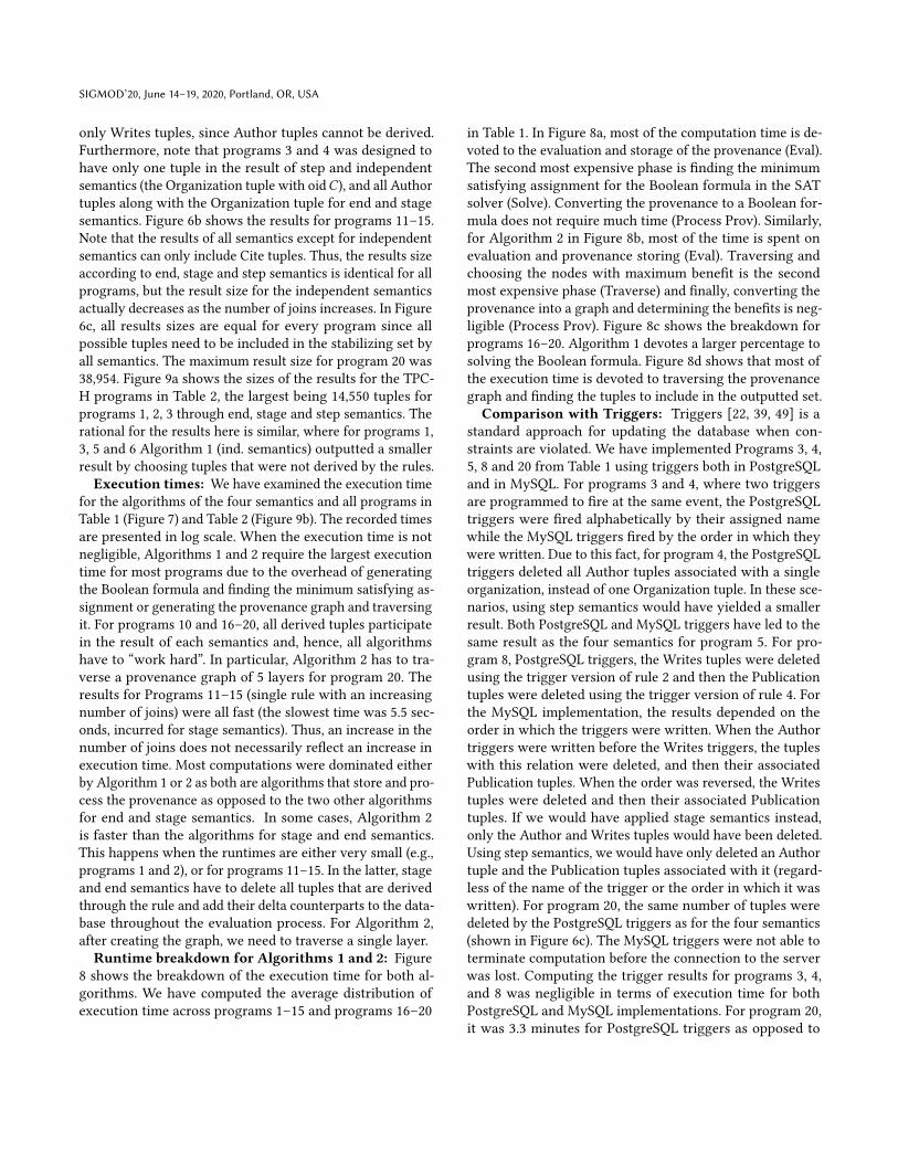
Table 4: Number of over deletions (+) for each of thefour semantics compared with number of under re-paired tuples (−) by HoloClean for an increasing thenumber of errors. Note that in contrast to HoloCleanall of our semantics always fixed all violations

Deleted Tuples Repaired TuplesErrors Ind Step Stage End HoloClean

100 +0 +0 +389 +389 -26200 +0 +1 +479 +479 -60300 +0 +5 +630 +630 -128500 +0 +16 +786 +786 -234700 +0 +21 +878 +878 -4801000 +0 +34 +1000 +1000 -693

Table 5: Number of tuples that violate a DCwith othertuples in the table after/before the repair for bothHoloClean and our four semantics. Some tuples partic-ipate in multiple violations

HoloClean SemanticsErrors DC1 DC2 DC3 DC4 Total Total

100 22/42 30/46 0/112 0/415 52/615 0/615200 42/82 78/110 0/208 0/563 120/963 0/963300 94/158 98/140 64/302 187/761 443/1361 0/1361500 134/254 116/246 218/500 464/1015 932/2015 0/2015700 198/320 182/364 580/716 872/1272 1832/2672 0/26721000 238/474 186/520 962/1006 1355/1612 2741/3612 0/3612

2.9 minutes for end semantics, and 4.25 minutes for stagesemantics, 40.3 minutes for step semantics, and 2.4 minutesfor the independent semantics.

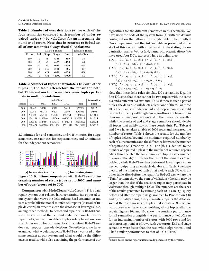
(a) Increasing #errors (b) Increasing #rowsFigure 10: Runtime comparison with HoloClean for in-creasing number of errors (rows set to 5000) and num-ber of rows (errors set to 700)

ComparisonwithHoloClean: HoloClean [44] is a datarepair system that relaxes hard constraints (as opposed toour system that views the delta rules as hard constraints) anduses a probabilistic model to infer cell repairs (instead of tu-ple deletions) in order to clean the database. It leverages DCs,among other methods, to detect and repair cells. HoloCleanuses the context of the cell and statistical correlations torepair cells, rather than delete tuples solely based on con-straints, as we do for our semantics. In addition, HoloCleandoes not support cascade deletion. Nevertheless, we haveexamined what would happen if HoloClean was used in thesame context as our system and what would be the differ-ence in results, while also examining the performance of our

algorithms for the different semantics in this scenario. Wehave used the code of the system from [1] with the defaultconfiguration that allows for a single table to be inputted.Our comparison used the Author table as presented at thestart of this section with an extra attribute stating the or-ganization name: Author(aid, name, oid, organization). Wehave used four DCs, expressed here as delta rules:(DC1) ∆A1 (a1,n1,o1,on1) :- A1(a1,n1,o1,on1),

A2(a2,n2,o2,on2), a1 = a2,o1 , o2(DC2) ∆A1 (a1,n1,o1,on1) :- A1(a1,n1,o1,on1),

A2(a2,n2,o2,on2), a1 = a2,n1 , n2(DC3) ∆A1 (a1,n1,o1,on1) :- A1(a1,n1,o1,on1),

A2(a2,n2,o2,on2), a1 = a2,on1 , on2(DC4) ∆A1 (a1,n1,o1,on1) :- A1(a1,n1,o1,on1),

A2(a2,n2,o2,on2), o1 = o2,on1 , on2Note that these delta rules simulate DCs semantics. E.g., thefirst DC says that there cannot be two tuples with the sameaid and a different oid attribute. Thus, if there is such a pair oftuples, the delta rule will delete at least one of them. For theseDCs, the results of independent and step semantics shouldbe exact in theory (although our algorithms are heuristic sotheir output may not be identical to the theoretical results),while the results of end and stage semantics should deleteall tuples that satisfy any of these constraints. For Tables 4and 5 we have taken a table of 5000 rows and increased thenumber of errors. Table 4 shows the results for the numberof tuples deleted beyond the minimum required number byeach of our semantics and the difference between the numberof repairs to cells made by HoloClean (this is identical to thenumber of repaired tuples) to the number of required repairs.Algorithm 1 deleted the same number of tuples as the numberof errors. The algorithms for the rest of the semantics ‘overdeleted’, while HoloClean has performed fewer repairs thanneeded2 outputting an unstable database. In Table 5 we havemeasured the number of tuples that violate each DC with an-other tuple after/before the repair for HoloClean, where the“Total” column shows the sum of violations (the sum may belarger than the size of the set, since tuples may participate inviolations through multiple DCs). The numbers are the sizesof the results generated by running each DC as an SQL querybefore and after the repair. As guaranteed by Proposition 3.18and by our algorithms, every semantics repairs the databaseso that there are no sets of tuples that violate a DCs, whereHoloClean may leave some violating sets of tuples after therepair. Figures 10a and 10b show the runtime performancefor all semantics alongside the performance of HoloCleanfor an increasing number of errors with 5000 rows and foran increasing number of rows with 700 errors. End and stagesemantics were faster than the rest, while Algorithms 1 and2 had similar performance to that of HoloClean.

2This is based on the report automatically generated by the system.


7 RELATEDWORKData repair. Multiple papers have used database con-straints as a tool for fixing (in our terms stabilizing) thedatabase [5, 6, 11, 19, 44]. The literature on data repair canbe divided by two main criteria: the types of constraintsconsidered and the methods to repair the database. A widevariety of constraints with different forms and functionshave been proposed. Examples include functional depen-dencies and versions thereof [8, 30], and denial constraints[10]. As we have discussed in Section 3.6, our model canexpress various forms of constraints, but our semantics al-low these constraints to be interpreted in different ways andnot operate according to one specific algorithm or approach.Regarding methods of data repair, previous works have con-sidered two main approaches: (1) repairing attribute valuesin cells [6, 11, 29, 33, 44] and (2) tuple deletion [10, 33, 34];our work focuses on the latter. A major advantage of ourapproach is the ability to perform cascade deletions overmultiple relations in the database while following differentwell-defined semantics (and the admin may choose whichone to follow based on the application scenario). Similar toour independent semantics, a common objective for datarepairs is to change the database in the minimal way thatwill make it consistent with the constraints [5, 19, 33]. Insome scenarios a good repair can be obtained by changingvalues in the database and the metric of minimal changesmay not work well [44]. However, in our approach as in[10], we assume that the starting database is complete, so theonly way to fix it is by deleting tuples and thus we use theminimum cardinality metric to achieve a repair following thedelta program; extending delta rules to updates of values isan interesting future work. Similar to our declarative repairframework by delta rules, declarative data repair has beenexplored from multiple angles [20, 21, 28, 43, 51]; e.g., [20]has focused on the rule-based framework of information ex-traction from text and includes a mechanism for prioritizedDC repairs, while [44] expresses constraints in DDlog [48].

Causality in databases. This subject has been the ex-plored in many previous works [36–38]. Works such as[45, 46] consider causal dependencies for explaining resultsof aggregate queries, that start their operation when there isan initial event of tuple deletion called “intervention” andrepair the database if a constraint is violated, e.g., [46] con-sidered repairs with respect to foreign keys in both ways(similar to rules (2) and (3) in Example 1.1). Delta programscan capture these as well as more complex cascaded deletionrules. Moreover, interventions can also be applied in ourframework, as we can add auxiliary rules to the programthat will start the deletion process.

Stable model. Stable model semantics [14, 24] is a wayof defining the semantics of the answer set of logic programs

with negation using the concept of a reduct. In stable models,if a tuple does not exist in the database, it means that itsnegation exists. In our model, ∆i is not the negation of Ri ,but is a record of deleted tuples from Ri . Also in our model,the head atom in each rule can only be a delta atom, ratherthan a positive atom as in stable model. Another relevantwork related to our framework is [23], where the authorsused the concept of stable models to solve the data conflictproblemwith trust mappings. Theway one’s belief is updatedfrom others’ beliefs is expressed by weighted update rulesthat are similar in spirit to our delta rules. However, unlikethe delta rules, in [23] rules have priorities, the results ofthe semantics can be computed in PTime under the skepticparadigm, and they have different usages.

Deletion propagation. Classic deletion propagation isthe problem of evaluating the effect of deleting tuples fromthe database D on the view obtained from evaluating a queryQ over D [18, 25, 26]. A more closely related variation isthe source side-effect problem [9, 12, 13], which focuses onfinding the minimum set of source tuples in D that has to bedeleted for a given tuple t ∈ Q(D) to be removed from theresult. Our approach may be combined with this problemby including the delta program as another input and solvingthe source side-effect problem given the delta program anda particular semantics.

8 CONCLUSIONS AND FUTUREWORKIn this paper, we presented a unified framework for data re-pair that involves deletions. We proposed delta rules to spec-ify the constraints on the data and four semantics that cap-ture behaviors inspired by DCs, a subset of SQL triggers, andcausal dependencies, allowing for different interpretationof the same set of constraints. We studied the relationshipsbetween these semantics and their complexity, proposedefficient algorithms, and evaluated them experimentally.We considered delta programs that are not inherently

recursive (Section 2). Although all definitions and complexityresults (in Sections 2, 3, and 4) apply to recursive programs,our algorithms for intractable cases cannot currently handlerecursive programs as for such programs the provenance sizemay be super-polynomial in the database size. Extendingour solutions to recursive programs is a future work. Otherfuture directions include extensions to updates in additionto deletions, and to soft and probabilistic constraints.

Acknowledgements. This research has been funded by the Eu-ropean Research Council (ERC) under the European Union’s Hori-zon 2020 research and innovation programme (Grant agreementNo. 804302), the Israeli Science Foundation (ISF) Grant No. 978/17,NSF awards IIS-1552538 and IIS-1703431, NIH award R01EB025021,and the Google Ph.D. Fellowship. The contribution of Amir Giladis part of his Ph.D. research conducted at Tel Aviv University.


REFERENCES[1] Code for holoclean. https://github.com/HoloClean/holoclean.[2] Serge Abiteboul, Meghyn Bienvenu, and Daniel Deutch. Deduction in

the presence of distribution and contradictions. In WebDB, 2012.[3] Serge Abiteboul, Daniel Deutch, and Victor Vianu. Deduction with

contradictions in datalog. In ICDT, pages 143–154, 2014.[4] Serge Abiteboul, Richard Hull, and Victor Vianu. Foundations of

Databases. Addison-Wesley, 1995.[5] Foto N. Afrati and Phokion G. Kolaitis. Repair checking in inconsistent

databases: Algorithms and complexity. In ICDT, pages 31–41, 2009.[6] Leopoldo E. Bertossi, Solmaz Kolahi, and Laks V. S. Lakshmanan. Data

cleaning and query answering with matching dependencies and match-ing functions. Theory Comput. Syst., 52(3):441–482, 2013.

[7] Nikolaj Bjørner, Anh-Dung Phan, and Lars Fleckenstein. ν z - anoptimizing SMT solver. In TACAS, pages 194–199, 2015.

[8] Philip Bohannon, Wenfei Fan, Floris Geerts, Xibei Jia, and Anasta-sios Kementsietsidis. Conditional functional dependencies for datacleaning. In ICDE, 2007.

[9] Peter Buneman, Sanjeev Khanna, and Wang Chiew Tan. On propa-gation of deletions and annotations through views. In PODS, pages150–158, 2002.

[10] Jan Chomicki and Jerzy Marcinkowski. Minimal-change integritymaintenance using tuple deletions. Inf. Comput., 197(1-2):90–121,2005.

[11] Xu Chu, Ihab F. Ilyas, and Paolo Papotti. Holistic data cleaning: Puttingviolations into context. In ICDE, pages 458–469, 2013.

[12] Gao Cong, Wenfei Fan, and Floris Geerts. Annotation propagationrevisited for key preserving views. In CIKM, pages 632–641, 2006.

[13] Gao Cong, Wenfei Fan, Floris Geerts, Jianzhong Li, and Jizhou Luo.On the complexity of view update analysis and its application to an-notation propagation. IEEE Trans. Knowl. Data Eng., 24(3), 2012.

[14] Evgeny Dantsin, Thomas Eiter, Georg Gottlob, and Andrei Voronkov.Complexity and expressive power of logic programming. ACMComput.Surv., 33(3):374–425, 2001.

[15] Leonardo Mendonça de Moura and Nikolaj Bjørner. Z3: an efficientSMT solver. In TACAS, pages 337–340, 2008.

[16] Daniel Deutch and Nave Frost. Constraints-based explanations ofclassifications. In ICDE, pages 530–541, 2019.

[17] Daniel Deutch, Amir Gilad, and Yuval Moskovitch. Selective prove-nance for datalog programs using top-k queries. PVLDB, 8(12):1394–1405, 2015.

[18] Daniel Deutch, Tova Milo, Sudeepa Roy, and Val Tannen. Circuits fordatalog provenance. In ICDT, pages 201–212, 2014.

[19] Ronald Fagin, Benny Kimelfeld, and Phokion G. Kolaitis. Dichotomiesin the complexity of preferred repairs. In PODS, pages 3–15, 2015.

[20] Ronald Fagin, Benny Kimelfeld, Frederick Reiss, and Stijn Vansum-meren. Declarative cleaning of inconsistencies in information extrac-tion. ACM Trans. Database Syst., 41(1):6:1–6:44, 2016.

[21] Helena Galhardas, Daniela Florescu, Dennis E. Shasha, Eric Simon, andCristian-Augustin Saita. Declarative data cleaning: Language, model,and algorithms. In VLDB, pages 371–380, 2001.

[22] Hector Garcia-Molina, Jeffrey D. Ullman, and Jennifer Widom. Data-base systems - the complete book (2. ed.). Pearson Education, 2009.

[23] Wolfgang Gatterbauer and Dan Suciu. Data conflict resolution usingtrust mappings. In SIGMOD, pages 219–230, 2010.

[24] Michael Gelfond and Vladimir Lifschitz. The stable model semanticsfor logic programming. In ICLP, pages 1070–1080, 1988.

[25] Todd J. Green, Gregory Karvounarakis, and Val Tannen. Provenancesemirings. In PODS, pages 31–40, 2007.

[26] Todd J. Green, Grigoris Karvounarakis, Zachary G. Ives, and Val Tan-nen. Update exchange with mappings and provenance. In VLDB, pages

675–686, 2007.[27] Aric Hagberg, Pieter Swart, and Daniel S Chult. Exploring network

structure, dynamics, and function using networkx. Technical report,Los Alamos National Lab, United States, 2008.

[28] Jian He, Enzo Veltri, Donatello Santoro, Guoliang Li, GiansalvatoreMecca, Paolo Papotti, and Nan Tang. Interactive and deterministicdata cleaning. In SIGMOD, pages 893–907, 2016.

[29] Solmaz Kolahi and Laks V. S. Lakshmanan. On approximating optimumrepairs for functional dependency violations. In ICDT, pages 53–62,2009.

[30] Nick Koudas, Avishek Saha, Divesh Srivastava, and Suresh Venkata-subramanian. Metric functional dependencies. In ICDE, 2009.

[31] Stefan Kratsch, Dániel Marx, and Magnus Wahlström. Parameterizedcomplexity and kernelizability of max ones and exact ones problems.TOCT, 8(1):1:1–1:28, 2016.

[32] Yi Li, Aws Albarghouthi, Zachary Kincaid, Arie Gurfinkel, and MarshaChechik. Symbolic optimization with SMT solvers. In POPL, pages607–618, 2014.

[33] Ester Livshits, Benny Kimelfeld, and Sudeepa Roy. Computing opti-mal repairs for functional dependencies. In SIGMOD-SIGACT-SIGAISymposium on Principles of Database Systems, pages 225–237, 2018.

[34] Andrei Lopatenko and Leopoldo E. Bertossi. Complexity of consistentquery answering in databases under cardinality-based and incrementalrepair semantics. In ICDT, pages 179–193, 2007.

[35] MAS. http://academic.research.microsoft.com/.[36] Alexandra Meliou, Wolfgang Gatterbauer, Joseph Y. Halpern,

Christoph Koch, Katherine F. Moore, and Dan Suciu. Causality indatabases. IEEE Data Eng. Bull., 33(3):59–67, 2010.

[37] Alexandra Meliou, Wolfgang Gatterbauer, Katherine F. Moore, andDan Suciu. WHY so? or WHY no? functional causality for explainingquery answers. In MUD, pages 3–17, 2010.

[38] Alexandra Meliou, Sudeepa Roy, and Dan Suciu. Causality and expla-nations in databases. PVLDB, 7(13):1715–1716, 2014.

[39] Jim Melton and Alan R Simon. SQL: 1999: understanding relationallanguage components. Elsevier, 2001.

[40] MySQL. Mysql trigger syntax. https://dev.mysql.com/doc/refman/8.0/en/trigger-syntax.html, 2019.

[41] Robert Nieuwenhuis and Albert Oliveras. On SAT modulo theoriesand optimization problems. In SAT, pages 156–169, 2006.

[42] PostgreSQL. Postgresql trigger behavior. https://www.postgresql.org/docs/12/trigger-definition.html, 2019.

[43] Nataliya Prokoshyna, Jaroslaw Szlichta, Fei Chiang, Renée J. Miller, andDivesh Srivastava. Combining quantitative and logical data cleaning.PVLDB, 9(4):300–311, 2015.

[44] Theodoros Rekatsinas, Xu Chu, Ihab F. Ilyas, and Christopher Ré.Holoclean: Holistic data repairs with probabilistic inference. PVLDB,10(11):1190–1201, 2017.

[45] Sudeepa Roy, Laurel Orr, and Dan Suciu. Explaining query answerswith explanation-ready databases. PVLDB, 9(4):348–359, 2015.

[46] Sudeepa Roy andDan Suciu. A formal approach to finding explanationsfor database queries. In SIGMOD, pages 1579–1590, 2014.

[47] Roberto Sebastiani and Silvia Tomasi. Optimization in SMTwith LA(Q)cost functions. CoRR, abs/1202.1409, 2012.

[48] Jaeho Shin, Sen Wu, Feiran Wang, Christopher De Sa, Ce Zhang, andChristopher Ré. Incremental knowledge base construction using deep-dive. PVLDB, 8(11):1310–1321, 2015.

[49] American National Standard. Information Systems Database LanguagesSQL Part 1/2: Framework/Foundation. American National StandardsInstitute, Inc., 1999.

[50] TPC. Tpc benchmarks, 2020.[51] Maksims Volkovs, Fei Chiang, Jaroslaw Szlichta, and Renée J. Miller.

Continuous data cleaning. In ICDE, pages 244–255, 2014.

https://github.com/HoloClean/holoclean

http://academic.research.microsoft.com/

https://dev.mysql.com/doc/refman/8.0/en/trigger-syntax.html

https://dev.mysql.com/doc/refman/8.0/en/trigger-syntax.html

https://www.postgresql.org/docs/12/trigger-definition.html

https://www.postgresql.org/docs/12/trigger-definition.html

On Multiple Semantics for Declarative Database Repairs

Documents

Transcript of On Multiple Semantics for Declarative Database Repairs