On modelling of postglacial gravity change - lantmateriet.se · postglacial land uplift and gravity...
49
Transcript of On modelling of postglacial gravity change - lantmateriet.se · postglacial land uplift and gravity...

On modelling of postglacial gravity change
PER-ANDERS OLSSONDepartment of Earth and Space SciencesChalmers University of Technology
Abstract
Glacial isostatic adjustment (GIA) is the Earth's response to glacial-inducedload variations on its surface. This phenomenon can today be observed in,for example, North America and Fennoscandia. Di�erent observables, suchas vertical and horizontal deformation of the crust, relative sea level changeand disturbances in the gravity �eld, contribute di�erent and complementalinformation on the phenomenon. Knowledge of the gravitational component isimportant for understanding the underlying geodynamical processes. Further,accurate predictions of the gravity change are important for e.g. reductions ofgeodetic observations to a reference epoch.
During the last decade, e�orts to observe the surface gravity change inFennoscandia have been intensi�ed and the observational accuracy successivelyimproved. This o�ers new possibilities at the same time as it puts new de-mands on modelling. The purpose of this thesis is to study some aspects of themodelling of GIA-induced gravity change.
We show that gravity stations close to the sea are a�ected by non-tidal sealevel variations and that the direct attraction from the sea water constitutes acrucial contribution. Accurate modelling of the direct attraction from sea wateris an intricate matter. We use di�erent methods to model the direct attrac-tion from GIA-induced sea level change and show that standard methods arenot adequate. Further we solve the forward GIA modelling problem and shownumerically how predictions of the gravity change are a�ected using di�erentapproximate methods. We also investigate the relation between gravity changeand vertical displacement as they are predicted with the earth model dependingon di�erent sets of structural and rheological parameters. A linear relation isused as a reference. Deviations from the linear approximation are small, es-pecially in Fennoscandia. The relation di�ers more between di�erent regionsincluded in the study than between di�erent earth models within each region.
The thesis also includes an overview of observational e�orts to determine thepostglacial land uplift and gravity change in Fennoscandia, as well as a generaldiscussion on some modelling issues that form the background for the motiva-tion of the thesis.
Keywords: Glacial Isostatic Adjustment, postglacial rebound, gravity change,sea level change
i

ii

List of appended papers
This thesis is based on the work contained in the following appended papers,referred to in the text.
I. Per-Anders Olsson, Hans-Georg Scherneck, and Jonas Ågren. E�ects ongravity from non-tidal sea level variations in the Baltic Sea. Journal ofGeodynamics, 48:151-156, 2009.
II. Per-Anders Olsson and Martin Ekman. Crustal Loading and GravityChange during the Greatest Storm Flood in the Baltic Sea. Small Publi-cations in Historical Geophysics, 19:1-10, 2009.
III. Per-Anders Olsson, Hans-Georg Scherneck and Jonas Ågren. Modellingof the GIA-induced surface gravity change over Fennoscandia. Journal ofGeodynamics, 61:12-22, 2012.
IV. Per-Anders Olsson, Glenn Milne, Hans-Georg Scherneck and Jonas Ågren.The relation between gravity rate of change and vertical displacement inpreviously glaciated areas. Submitted to Journal of Geodynamics.
iii

iv

Acknowledgements
I would like to address the greatest thanks and appreciation to my supervisorsHans-Georg Scherneck for constant support, valuable guidance, challenging al-lures and always encouraging words, and Jonas Ågren for excessive engagementand long and fruitful discussions - without You this work would not have beenpossible. In the �nal stage Holger Ste�en enriched our group. I wish this hadhappened earlier.
Via the Training School on GIA Modelling, organized by the COST ActionES0701 in 2009, I was �rst introduced to GIA modelling, on which the majorpart of this dissertation relies.
I would also like to thank Lantmäteriet for giving me the opportunity to doresearch and increase my knowledge within this �eld. I appreciate that a lot.
Finally,Mom and Dad, thank you for everything,Lisa, Johanna, Jakob, Ida and Märta - you are the best.Love you all!
v

vi

Contents
Abstract i
List of appended papers iii
Acknowledgements v
1 Introduction 1
1.1 Background . . . . . . . . . . . . . . . . . . . . . . . . . . . . . . 21.2 Purpose and structure of the dissertation . . . . . . . . . . . . . 4
2 Observational e�orts 5
2.1 Empirical land uplift modelling (from geodetic observations) . . . 52.2 The Nordic Geodetic Commission . . . . . . . . . . . . . . . . . . 62.3 Fennoscandian land uplift gravity lines . . . . . . . . . . . . . . . 72.4 Nordic absolute gravity project . . . . . . . . . . . . . . . . . . . 82.5 BIFROST . . . . . . . . . . . . . . . . . . . . . . . . . . . . . . . 9
3 Modelling 11
3.1 Empirical and geophysical models . . . . . . . . . . . . . . . . . . 113.2 GIA modelling concepts . . . . . . . . . . . . . . . . . . . . . . . 163.3 Examples of GIA modelling e�orts in Fennoscandia . . . . . . . . 183.4 Benchmarking . . . . . . . . . . . . . . . . . . . . . . . . . . . . . 203.5 GIA-induced gravity change . . . . . . . . . . . . . . . . . . . . . 223.6 Prerequisites for this dissertation . . . . . . . . . . . . . . . . . . 24
4 Summary and conclusions 27
4.1 Paper I: E�ects on gravity from non-tidal sea level variations inthe Baltic Sea. . . . . . . . . . . . . . . . . . . . . . . . . . . . . 27
4.2 Paper II: Crustal loading and gravity change during the greateststorm �ood in the Baltic Sea. . . . . . . . . . . . . . . . . . . . . 27
4.3 Paper III: Modelling of the GIA-induced surface gravity changeover Fennoscandia. . . . . . . . . . . . . . . . . . . . . . . . . . . 28
4.4 Paper IV: The relation between gravity rate of change and verti-cal displacement in previously glaciated areas. . . . . . . . . . . . 29
4.5 Complementing remark . . . . . . . . . . . . . . . . . . . . . . . 30
5 Final words and recommendations 31
References 35
vii

viii

1 Introduction
Glacial cycles have come and gone with a period of approximately 100,000 years.The last glacial cycle started about 110,000 years ago when the climate turnedcolder and continental ice sheets started to grow, especially in the northernhemisphere. Around 20,000 years ago they reached their maximum, known aslast glacial maximum (LGM) (Figure 1). Then warmer climate led to a relativelyquick melting of the ice and some 8000 years ago the massive ice sheets in NorthAmerica, Fennoscandia and Barents-Kara-Seas were gone. The amount of frozenwater that was stored in the melted continental ice sheets and further mountainglaciers, if evenly distributed over the oceans, would correspond to a global sealevel rise of ∼ 130 meters.
LGM ice thickness (ICE5G)
180˚ 270˚ 0˚ 90˚ 180˚
0˚
LGM ice thickness (ICE5G)
180˚ 270˚ 0˚ 90˚ 180˚
0˚
0
00
0
0
0
0
0
0
01000
1000
1000
1000
1000
1000
1000
2000
2000
2000
2000
2000
2000
3000
3000
3000
4000
5000
0
1000
2000
3000
4000
5000
6000meter
Figure 1: Thickness of continental ice sheets at last glacial maximum accordingto the ice model ICE-5G (Peltier, 2004).
Under the load of the ice, the Earth was deformed, the surface was depressed,and when the load disappeared the Earth started to rebound. This postglacialrebound, or glacial isostatic adjustment (GIA), is still going on and can bestudied in e.g. North America and Fennoscandia.
There are two main reasons why we are interested in the GIA phenomenon:(1) we have to deal with its direct consequences, such as the ongoing deformationof the surface of the Earth, changing coastlines, and changes in the stress state ofthe crust that may lead to earthquakes;(2) by studying GIA we gain knowledgeof the phenomenon as such, of the ice history and of the physical structure ofthe Earth.
1
1.1 Background
This dissertation is the result of a cooperation between Lantmäteriet (the Swedishmapping, cadastral and land registration authority) and Chalmers University ofTechnology.
Lantmäteriet is responsible for the geodetic infrastructure in Sweden. Thisresponsibility includes establishment and maintenance of geodetic reference framesfor gravity and positioning. Since Sweden is located in the centre of the Fennoscan-dian postglacial rebound area, the e�ects of postglacial rebound have to beconsidered when designing, maintaining and using geodetic reference frames.In the strategic plan for Lantmäteriet's geodetic activities 2011-2020 (Lantmä-teriet, 2011), it is stated that:
"In our part of the world we have land uplift as a result of the latestice age. - - - In addition to its scienti�c value, the knowledge of theseprocesses is of considerable value for the maintenance of our nationalreference systems. - - - We have - - - an international responsibilityto provide researchers with the best possible geodetic observations- primarily GNSS observations at permanent reference stations aswell as gravity changes."
"We plan to - - - extend our R&D activities concerning geophysics-based models for land uplift. Further develop theories and methodsfor implementing deformation models in the maintenance of our ref-erence systems."
"Lantmäteriet's geodetic activities mirror a strong and genuine in-terest for continuing and increasing cooperation with Onsala SpaceObservatory."
Onsala Space Observatory, located south of Gothenburg in Sweden, is theSwedish National Facility for Radio Astronomy and an important geodetic fun-damental station. It is hosted by the Institution for Earth and Space Science atChalmers University of Technology. Besides an extensive equipment park for as-tronomical purposes, the observatory also conducts research related to geodesyand geodynamics and provides e.g. VLBI (very long baseline interferometry),GNSS (global navigation satellite system) and gravity observations for scienti�cpurposes.
Gravity is, among many others, an important observable of postglacial re-bound. It contributes with unique information on the underlying physics, suchas the redistributions of masses within the Earth, as well as information on thelocation of the centre of mass (CM) of the Earth.
During the �rst years of the 21st century, the activity concerning absolutegravity (AG) observations of the GIA-induced gravity change in Fennoscandiaincreased. Various institutions contributed with observations, coordinated bythe Nordic geodetic commission (NKG) (see Section 2.4). In 2006, Lantmäterietinvested in an FG5 absolute gravimeter. One of the main purposes with this in-vestment was to contribute to, continue and ensure long time series of repeated
2

observations of the GIA-induced absolute gravity change. About the same timeChalmers installed a superconducting gravimeter (SG) at Onsala Space Obser-vatory, capable of measuring temporal changes in the gravitational �eld of theEarth at the 10−10 level, or 0.1 part per billion (Virtanen, 2004). With thesenew possibilities to observe gravity variations, a need to strengthen the knowl-edge related to GIA modelling and gravity change was recognized. What dowe observe and why? Chalmers and Lantmäteriet decided to establish a PhDposition, led by Chalmers and �nanced by Lantmäteriet. This dissertation isthe result of that PhD position.
The mobilization of new resources for observations of the GIA-induced grav-ity change was not intended to be a standalone e�ort, but should be seen asan integrated part of a very long tradition of observations of the postglacial re-bound in Fennoscandia. Scienti�c observations of the land uplift in Fennoscan-dia started with relative sea level observations in the 18th century and wassupplemented with repeated national levelling campaigns during the 20th cen-tury . Since the 1990's, a network of permanent GNSS stations is monitoring thethree-dimensional deformation of the crust. The GIA-induced gravity changewas �rst observed with repeated relative gravity campaigns during the secondhalf of the 20th century. During the last decades they have gradually been su-perseded by repeated absolute gravity observations. These observational e�ortsform the basis for what we know about the postglacial rebound in Fennoscandiatoday and in Section 2 they are described in more detail.
An increasing amount of observations of di�erent kinds of GIA observables,emphasize the question of how to relate and combine them. Relative sea levelobservations, by means of mareographs, measure the vertical displacement ofthe crust relative to the sea level; with repeated levelling campaigns the verticaldisplacement is measured relative to the geoid; permanent GNSS stations mea-sure the deformation of the crust relative to a global geodetic reference frame(e.g. ITRF), and inferences of the vertical deformation of the crust from re-peated observations of the surface gravity, are made relative to the centre ofmass of the Earth. Another issue related to the interpretation of the observa-tions, is how to interpolate between discrete observations, in time and space.These problems are preferably dealt with using appropriate modelling methods.In Section 3 we deepen the reasoning around these questions in general anddiscuss di�erent modelling approaches.
Observations and modelling of the GIA-induced surface gravity change, inparticular, are coupled to some speci�c questions related to the complex compo-sition of the signal. The gravity signal is a compound of contributions from e.g.redistribution of masses within the Earth, vertical displacement of the crust,redistribution of GIA-related masses on the surface of the Earth (ice and water)and external e�ects. With external e�ects we mean redistributions of massesnot related to GIA, such as e.g. sea level variations, continental water (groundwater) variations and atmospheric pressure. The complex nature of the grav-ity signal should be recognized when observations and modelled predictions areinterpreted.
3

1.2 Purpose and structure of the dissertation
The purpose of this dissertation is to contribute to the understanding of observedsurface gravity changes, the composition of the signal, how it is accuratelymodelled, and how it is related to the vertical deformation of the crust. Focusis mainly on Fennoscandia although most of the conclusions are general forall previously glaciated areas with postglacial rebound. The main results arepresented in four appended articles dealing with (I) the e�ect on gravity fromnearby sea level variations, (II) a case study of the e�ects on gravity from anextremely large sea level change, (III) how sensitive predictions of the rate ofchange of gravity are to some modelling assumptions and approximations and�nally (IV) the relation between the rate of change of gravity and the verticaluplift rate. A summary of the appended articles and the main conclusions aregiven in Section 4.
The purpose of Sections 2-3 is to put the articles in a historical and scienti�ccontext. Section 2 is a short introduction to important observational e�orts tostudy the postglacial rebound phenomena in Fennoscandia. Section 3 dealswith modelling and highlights some issues, related to modelling, that motivatesthis dissertation. Finally, in Section 5, we give some conclusive comments andsuggestions for future work.
4
2 Observational e�orts
In Fennoscandia, the postglacial rebound has been studied for a few hundredyears starting with relative sea level observations in the 18th century. The reasonbehind the observed relative sea level fall (or land uplift) was initially underdebate but during the second half of the 19th century the idea of postglacialrebound, �rst suggested by Jamison (1865), became generally accepted. VeningMeinesz (1934) and Haskell (1935) used uplift data from Fennoscandia to dothe �rst estimates of the viscosity of the mantle. For a thorough review ofthe early history of modelling and observations of GIA see e.g. Ekman (2009).During the 20th century the accuracy of land uplift observations has increasedby means of longer time series as well as the introduction of other/new typesof observational techniques, such as e.g. repeated levellings and during thelast decades continuous GNSS observations and repeated gravity observations.Modelling of the GIA phenomenon has developed and is now able to predictGIA observables, such as the rate of land uplift or relative sea level change, onthe millimeter/year level, or better.
The purpose with this section is to give an overview of important e�ortsto determine and study the postglacial rebound in Fennoscandia. Since themiddle of the 20th century, much of this work have been coordinated by theNordic Geodetic Commission and therefore one subsection is dedicated to a shortdescription of this association. The whole section will serve as the backgroundfor understanding where we are today. It is also the basis for the discussions inthe next section concerning issues related to the choice of appropriate modellingapproaches and for what we can expect from our observations of the surfacegravity change. A comprehensive review of data and modelling in Fennoscandiacan be found in Ste�en and Wu (2011).
2.1 Empirical land uplift modelling (from geodetic obser-vations)
For many hundred years, people in Scandinavia, inhabiting the coastlines, havebeen observing the postglacial land uplift in terms of relative sea level decrease.In the early 18th century the Swedish astronomer and geodesist, Anders Celsius(1701-1744), started scienti�c investigations of the phenomenon based on sealevel observations. Since the late 19th century the sea level relative to the solidcrust have been recorded at a large number of sea level stations around theBaltic Sea. Some 30 of these stations have continuous sea level records spanningover 100 years (Ekman, 1996) and one station, Stockholm, is spanning over 200years and thereby constitute the world's longest sea level series (Ekman, 2003).Thorough descriptions of the historical land uplift research in this region is givenby in Ekman (1991) and Ekman (2009).
During the last century repeated national levellings in the Nordic countrieshave been performed and thereby observations of land uplift have been extendedfrom the coastline to the inland. Mäkinen and Saaranen (1998), for example,determine the postglacial land uplift from three precise levellings in Finland.
5

Figure 2 shows an, often referred to, land-uplift map constructed by Ekman(1996) from a combination of sea and lake level records and repeated levelling.
Figure 2: Empirical model of the apparent land uplift (relative to sea level) basedon sea and lake level records and repeated levellings (Ekman, 1996). Dashedlines indicate interpolation, made by the author, between observations.
2.2 The Nordic Geodetic Commission
The Nordic Geodetic Commission (NKG) is an association, founded in 1953,recognized and supported by a number of organizations in the Nordic coun-tries (Denmark, Finland, Iceland, Norway and Sweden), such as universitiesand national mapping authorities. The purpose of this association is to pro-mote research, data exchange and cooperation between geodesists in the Nordic
6

countries. Organizations from neighboring countries, such as the Baltic coun-tries, Germany and Poland, occasionally participate in projects coordinated byNKG.
The NKG, acknowledging the importance of gravity change as a geodeticand scienti�c problem, delegated the responsibility to measure the phenomenonto a dedicated Working Group of Geodynamics, which has devoted its e�ortsin studying the e�ects within a broad range of questions and methods, likeobtaining accurate earth tide models, agreeing on data reduction algorithms,looking into alternative kinds of instrumentation like water tube tiltmeters.The group started its work in 1967 and is still active.
The empirical land uplift model of NKG, NKG2005LU (bottom panel inFigure 8), is based on geodetic observations (Ågren and Svensson, 2007; Vestøl,2006). In addition to sea level observations and repeated levelling, it includesGNSS observations from the BIFROST-network (see section 2.5) and also makeuse of a geophysical land uplift model by Lambeck et al. (1998) (see section3.3) for extrapolation outside the observations. NKG2005LU was used in theadjustment of the new national height systems in Sweden (RH2000), Finland(N2000) and Norway (NN2000) as well as in the latest realization of the Euro-pean Vertical Reference System, i.e. EVRF2007 (Sacher et al., 2008).
2.3 Fennoscandian land uplift gravity lines
A major project that was initiated and coordinated by NKG are the Fennoscan-dian land uplift gravity lines. They consist of four east-west high precisionrelative gravity pro�les across the Fennoscandian postglacial rebound area, ap-proximately following the latitudes 65◦, 63◦, 61◦ and 56◦N (Figure 3) (Mäkinenet al., 1986). Measurements along the Finnish part of the 63◦ line started in1966 (Kiviniemi, 1974) followed by the rest of the lines from the mid 1970s.
At the time of the establishment of the land uplift gravity lines, the geo-metrical land uplift was relatively well known from sea level observations andrepeated levelling campaigns (section 2.1). The purpose of the gravity measure-ments was to determine the rate of change of gravity, g, and compare this withthe absolute land uplift rate, u. From the ratio g/u, conclusions could then bereached concerning the underlying geodynamic processes (Kiviniemi, 1974).
From these observations Ekman and Mäkinen (1996) found the ratio be-tween the rate of change of gravity g and the land uplift rate u to be −0.204±0.058 µGal mm−1 (1 Gal = 0.01 m/s2). This was later revised by Mäkinenet al. (2005), based on longer time series, to be between -0.16 and -0.20 µGalmm−1. Based on this ratio and a number of approximations, for instance thatthe gravity change due to the mass �ow in the mantle can be properly describedby means of one planar Bouguer plate, they made the conclusion that the GIAprocess in Fennoscandia includes in�ow of additional mantle masses.
7

10˚
10˚
20˚
20˚
30˚
30˚
55˚
55˚
60˚
60˚
65˚65˚
70˚70˚
10˚
10˚
20˚
20˚
30˚
30˚
55˚
55˚
60˚
60˚
65˚65˚
70˚70˚
Figure 3: Red dots and lines show the Fennoscandian land uplift gravitylines (Mäkinen et al., 2005). Black dots show absolute gravity stations in theNKG/AG-network and white dots the superconducting gravimeter stations.
2.4 Nordic absolute gravity project
During the last decades the relative gravity observations have been succeededby absolute gravity (AG) observations.
The history of absolute gravity observations in Fennoscandia (Mäkinen et al.,2010) starts with six stations observed with the Italian instrument IMGC byIstituto de Metrologia (Turino) in 1978 and two stations with the GABL instru-ment by USSR Academy of science in 1980.
From 1988 (-2002) the Finnish Geodetic Institute (FGI) carried out repeatedmeasurements in Finland with a JILAg instrument and 1993 and 1995 the Na-tional Oceanic and Atmospheric Administration (NOAA), USA, and Bunde-
8

samt für Kartographie und Geodäsie (BKG), Germany, observed a number ofstations with the successor instrument FG5 (free fall gravimeter manufacturedby Micro-g Lacoste Inc., Colorado USA) (Niebauer et al., 1995).
In 2003 - 2008 comprehensive campaigning was carried out with an FG5 in-strument by Institute für Erdmessung (IfE), Germany (Gitlein, 2009). Duringthat time also FGI, Norwegian University of Life Sciences (UMB) and Lantmä-teriet (the Swedish mapping, cadastral and land registration authority) investedin FG5 gravimeters and started with repeated AG observations. This work, here-after referred to as the Nordic absolute gravity project, has been coordinatedby NKG. The observations are performed in the so-called NKG/AG-network,consisting of a number of stations suitable for AG observations, shown in Figure3. Most of the stations are co-located with permanent GPS-stations (see Section2.5 below) and some of them with tide gauges.
At present observations in the NKG/AG-network are carried out repeatedlyon the stations by FGI, UMB and Lantmäteriet and occasionally by IfE andBKG. The stations are intended to be reoccupied with one or a few years inter-vals. One long-term goal (10-30 years) of this project is a high accuracy modelof the GIA-induced gravity change for Fennoscandia. Another goal is to con-tribute with observations to the GIA modelling research in the area. A subsetof the AG stations is also planned to be used to establish new gravity referencesystems in the future.
Within the area two superconducting gravimeters are installed. One at On-sala in Sweden (operated by Chalmers University of Technology) and one atMetsähovi in Finland (operated by FGI) (Virtanen, 2006). They complementthe Nordic absolute gravity project with continuous observations of the gravitychange providing an excellent possibility to study external e�ects from e.g. vari-ations in atmospheric pressure, ocean load and continental water storage. Theyalso serve as suitable stations for comparisons between absolute gravimeters.
2.5 BIFROST
The BIFROST (Baseline Inference for Fennoscandian Rebound) project was ini-tiated 1993. With a network of permanent GNSS reference stations in Fennoscan-dia, the three-dimensional deformation of the crust is continuously measured.The network originally consisted of the Swedish (SWEPOS) and Finnish (FinnRef)national permanent GPS networks, established in 1991-1992 and 1994-1996, re-spectively. Later solutions also include stations in Norway (SATREF), Denmarkand a selection of stations in northern Europe (Lidberg et al., 2010) (Figure 4).In Scherneck et al. (2002) a thorough description of the network and its historyis given.
Solutions of the three-dimensional rates at the stations in the BIFROSTnetwork have been published in a number of articles, e.g. Johansson et al.(2002) and Lidberg et al. (2007, 2008, 2010). The results from Lidberg et al.(2010) are presented in Figure 4. Also a number of geophysical investigations,based on these BIFROST solutions, have been published, e.g. GIA modelling(see further Chapter 3.3) and inferences on the mantle viscosity pro�le by Milne
9

et al. (2001, 2004) and Hill et al. (2010) and determination of a Fennoscandianstrain rate �eld by Scherneck et al. (2010). Milne et al. (2004) also concludedthat BIFROST data provide distinct constraints on mantle viscosity. As afunction of depth in the mantle the resolving power varies from ∼ 200 km to∼ 700 km but provide little constraint on viscosity in the bottom half of themantle (Milne et al., 2004).
0˚ 10˚ 20˚ 30˚
50˚
55˚
60˚
65˚
70˚
0˚ 10˚ 20˚ 30˚
50˚
55˚
60˚
65˚
70˚
0˚ 10˚ 20˚ 30˚
50˚
55˚
60˚
65˚
70˚
ALES
ARJ0
BODS
BOGIBOGOBOR1
BORK
BRGS
BRUS
BUDP
DAGS
DENT
DLFT
DOMS
DRES
GOPE
HAS0
HELG
HERSHERT
HOBU
IRBE
JOEN
JON0
JOZ2JOZE
KAR0
KEVO
KIR0KIRU
KIVE
KLOP
KOSG
KRAW
KRSS
KUUS
LAMA
LEK0
LOV0
MAR6METS
NOR0
OLKI
ONSAOSK0
OSLS
OST0
OULU
OVE0
POTSPTBB
RIGA
ROMU
SASS
SKE0
SMID
SMO0
SODA
SPT0
STAS
SULD
SULP
SUN0
SUUR
SVE0
SVTL
TRDS
TRO1TROM
TRYS
TUOR
UME0
UPP0
VAAS
VAN0
VARS
VIL0
VIRO
VIS0
VLNS
WROC
WSRT
WTZR
. ..
INVE
MORP
0˚ 10˚ 20˚ 30˚
50˚
55˚
60˚
65˚
70˚
0˚ 10˚ 20˚ 30˚
50˚
55˚
60˚
65˚
70˚
0˚ 10˚ 20˚ 30˚
50˚
55˚
60˚
65˚
70˚
0˚ 10˚ 20˚ 30˚
50˚
55˚
60˚
65˚
70˚
10 mm/yr
1 mm/yr
Figure 4: The BIFROST velocity �eld from Lidberg et al. (2010). The legendshows 10 mm/year in the vertical and 1 mm/year in horizontal components.
10

3 Modelling
All observations, of various kinds, of the glacial isostatic adjustment are inter-preted by means of models (Figure 5). The physical prerequisites that controlthe GIA phenomenon, however, are too many and too complex to be understoodand described in detail. We make sampled observations, associated with errors,and develop simpli�ed models based on assumptions and approximations.
OObseervations Moodelss
Figure 5: Observations are interpreted with models. Models are improved,revised, con�rmed or rejected by observations.
In this section we discuss and give examples of some di�erent types of modelsof relevance for GIA research in Fennoscandia. We make a distinction betweenempirical models and geophysics-based GIA models, we also emphasize somespeci�c issues related to the GIA-induced gravity change. The purpose withthis section is to substantiate and illustrate some issues discussed within theNordic geodetic community during the last decade. These issues were importantas a motivation for this PhD thesis. We end this section with a summary ofprerequisites for this dissertation.
3.1 Empirical and geophysical models
Within NKG, and in this dissertation, the term empirical model occurs. Withempirical model we mean a model whose purpose is to compile observationsto get a uni�ed picture of the same phenomenon that we observe (Figure 6).These models are typically based on carefully evaluated observations and sta-tistical methods to �lter out unwanted errors and to interpolate between thesample observations. Empirical models describe a certain observable (e.g. rel-ative sea level change) and do not discriminate between di�erent mechanismsthat contribute to the total signal (e.g. vertical displacement of the crust, geoidchange and change in ocean volume). The term empirical model sometimesrefers to the predictions themselves ("Output" in Figure 6), e.g. gridded val-ues of the land uplift rate, rather than the underlying observations and the
11

OutputFilter/
InterpolationInput
Observations
Figure 6: Empirical model.
mathematical methods used. Although empirical models do not explain theunderlying mechanisms that cause the phenomenon that is observed, they areuseful for practical geodetic purposes. In Fennoscandia, empirical models of theland uplift rate (Section 2.1) have typically been used to reduce observationsfrom di�erent time epochs to a common reference epoch.
In Figure 7 two examples of empirical models are presented. One is anestimated trend of the relative sea level change in Stockholm. From annualmeans of relative sea level observations (Ekman, 2003, 2009), the trend hasbeen estimated by means of linear regression. Unwanted short-term variationshave been �ltered out and the estimated trend (empirical model) can be usedto predict annual mean sea level in Stockholm at an optional time.
The other model in Figure 7 is more complex. It is a compilation of di�erenttypes of observations of the land uplift in Fennoscandia. Repeated levelling,tide gauge observations and continuous GNSS observations have been combinedand evaluated by means of least squares collocation (Vestøl, 2006). This modelwas developed as one important step towards an o�cial NKG land uplift model,urged for construction of new national and regional height systems in the Nordicare (see e.g. Sacher et al., 2008; Ågren and Svensson, 2007).
The empirical models discussed above are based on observations and math-ematical/statistical methods. Insights in physical conditions and constraintsmight indicate shortcomings of these models - or help to improve them. Thetop panel in Figure 8 shows the same data set as the top panel in Figure 7.Now two regression lines have been used to estimate the relative sea level trend,one for the years 1774-1865 (the dashed line is an extrapolation of this trendto year 2000), and one for the years 1865-2000. This approach is based on theassumption that since 1865 the local, GIA-induced relative sea level change hasbeen complemented by a global increase of the ocean volume, induced by globalwarming as a result of the industrial revolution, resulting in decreased relativesea level trend in Stockholm.
12

175
200
225
250
275
300
1750 1800 1850 1900 1950 2000
RS
L [c
m]
Year
36
10° 20° 30°
40°
50°50°
55°55°
60°60°
65°65°
70° 70°
4
6
6
8
10° 20° 30°
40°
50°50°
55°55°
60°60°
65°65°
70° 70°
−3
−2
−1
0
1
2
3
4
5
6
7
8
9mm/year
Figure 2.11: Contour lines for the apparent land uplift of Vestøl's grid model. Zero uplift is plotted where the model is undefined. Unit: mm/year. Table 2.3: Statistics for the apparent uplift residuals for Vestøl‘s grid model. The maximum for “All tide gauges” is given for both the outlier stations discussed in the text (Furuögrund/Oslo). Unit: mm/year.
Observations # Min Max Mean StdDev RMS
All tide gauges 58 -0.19 0.88/1.20 0.04 0.20 0.20
Cleaned tide gauges 56 -0.19 0.18 0.00 0.08 0.08
All GPS 55 -1.27 1.53 -0.02 0.45 0.45
SWEPOS GPS 21 -0.56 0.31 -0.03 0.23 0.23
It is clear that Vestøl model behaves as could be expected. It fits extraordinarily well to the tide gauges, which of course depends on the very high weight given to these observations; cf. Table 2.2. The fit to the SWEPOS stations is further good and the accuracy degrades when all GPS stations are considered, exactly as indicated by the
Figure 7: Two examples of empirical models; the top model is a straight linerepresenting the relative sea level change in Stockholm (Ekman, 2003, 2009),found from linear regression of annual means of tide gauge observations; thebottom model bottom is a land uplift model, based on least squares collocationof di�erent types of observations (Vestøl, 2006; Ågren and Svensson, 2007).
13

175
200
225
250
275
300
1750 1800 1850 1900 1950 2000
RS
L [c
m]
Year
Figure 8: The same empirical models as in in Figure 7 but now re�ned basedon insights in physical conditions and constraints (see text).
14
Further, the Vestøl model in the bottom panel in Figure 7 also raises somequestions related to the underlying physics. Are the irregularities in the iso-lines physically relevant or are they caused by observational errors? How do weextrapolate outside the area covered by observations? These questions demon-strate some limitations with purely empirical models. In order to overcomethese limitations Ågren and Svensson (2007) applied smoothing algorithms tothe Vestøl (2006) model and combined it with a geophysics-based GIA model(see Section 3.2) of Lambeck et al. (1998) (see Section 3.3). This resulted inthe o�cial NKG land uplift model NKG2005LU shown in the bottom panel inFigure 8 (see also Section 2.2). This model can be regarded as a mix of anempirical model and di�erent physical assumptions.
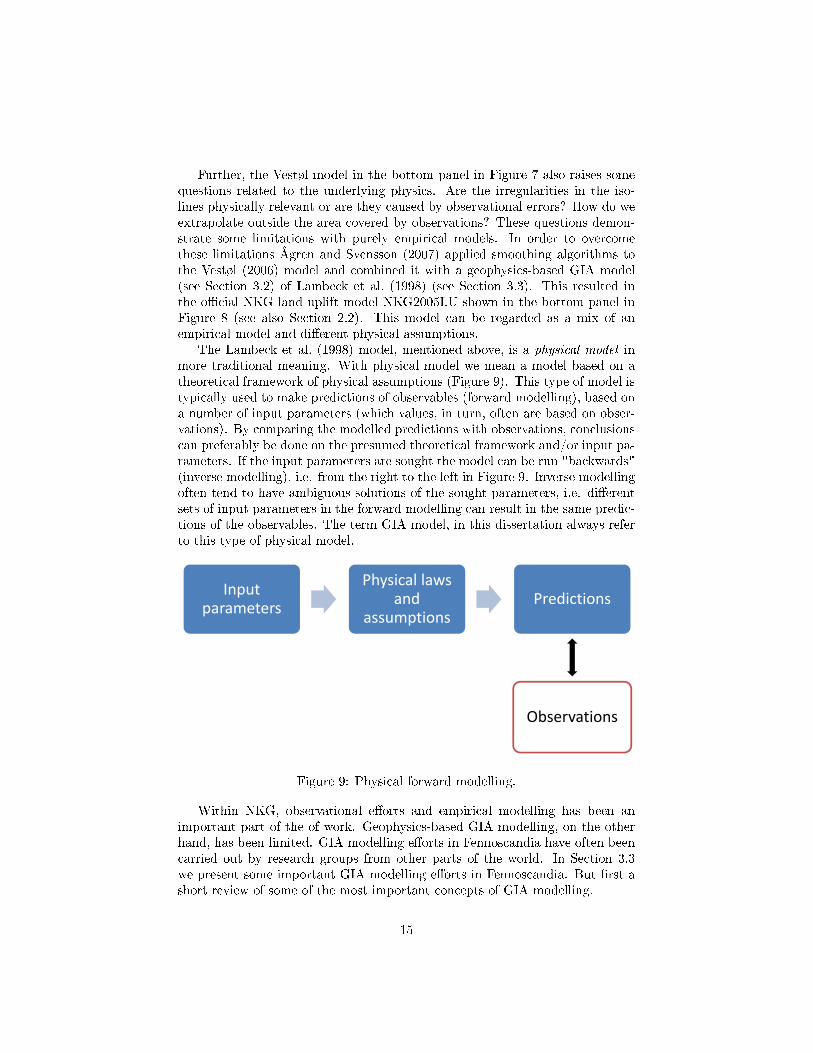
The Lambeck et al. (1998) model, mentioned above, is a physical model inmore traditional meaning. With physical model we mean a model based on atheoretical framework of physical assumptions (Figure 9). This type of model istypically used to make predictions of observables (forward modelling), based ona number of input parameters (which values, in turn, often are based on obser-vations). By comparing the modelled predictions with observations, conclusionscan preferably be done on the presumed theoretical framework and/or input pa-rameters. If the input parameters are sought the model can be run "backwards"(inverse modelling), i.e. from the right to the left in Figure 9. Inverse modellingoften tend to have ambiguous solutions of the sought parameters, i.e. di�erentsets of input parameters in the forward modelling can result in the same predic-tions of the observables. The term GIA model, in this dissertation always referto this type of physical model.
Input parameters
Physical laws and
assumptionsPredictions
Observations
Figure 9: Physical forward modelling.
Within NKG, observational e�orts and empirical modelling has been animportant part of the of work. Geophysics-based GIA modelling, on the otherhand, has been limited. GIA modelling e�orts in Fennoscandia have often beencarried out by research groups from other parts of the world. In Section 3.3we present some important GIA modelling e�orts in Fennoscandia. But �rst ashort review of some of the most important concepts of GIA modelling.
15

3.2 GIA modelling concepts
With GIA model we mean a geophysics-based model (Figure 10). GIA mod-elling normally consists of an ice- and an earth model and a number of phys-ically meaningful constitutive equations that control how the Earth reacts onthe surface loading from the ice. The GIA model then predicts e.g. crustaldeformation, gravity disturbances, sea level variations and/or disturbances ofthe Earth's rotational vector (Figure 10). This section is a short presentation ofsome fundamental concepts related to GIA modelling which are of importancefor the following discussions. A state of the art report of GIA theory is givenby Whitehouse (2009).
Inpnput arameter
•Ice m
•Eart
rs
model
h model
Theorframe
•
•
retical ework
•Constituequation
•Methodsolution
utive ns
of s
PPredictio
•Crudef
•Gradist
•Relleve
•Eardist
ns
ustal formation
avity turbances
ative sea el change
rth rotatioturbances
n
s
e
on s
Figure 10: GIA model.
The ice model describes the thickness of the ice (the load) and is allowed tovary in time and space. Depending on the premises under which the ice modelhas been constructed it can be categorized as geophysics-based or climate driven.
Geophysics-based ice models are constructed by means of GIA modellingand are typically tuned to geological constraints like ancient sea level indicators.Examples of important geophysics-based ice models are the series of consecutiveglobal models ICE-3G (Tushingham and Peltier, 1991), ICE-4G (Peltier, 1994,1996) and ICE-5G (Peltier, 2004) and the regional model, explicitly tuned toobservations in Fennoscandia, by Lambeck et al. (1998). The regional modelis also a part of global model consisting of a compilation of regional models.Further, the ICE-5G model has a successor, ICE-6G, but at the time of thiswriting it has not yet been published.
Climate driven ice models are based on thermo-dynamical ice sheet modelsdriven by paleoclimate data. The so-called Näslund ice model (SKB, 2010,Figure 11) is an example of a climate driven model for Fennoscandia.
The physical properties of the earth model are de�ned by a set of parameters,e.g. density, rigidity and viscosity, which are allowed to vary in one, two or threedimensions. A set of constitutive equations, fundamental physical laws, thengoverns how the earth model reacts to the surface loading. Depending on the
16

182 H. Steffen, P. Wu / Journal of Geodynamics 52 (2011) 169– 204
Fig. 12. Selected examples of trend estimates [�Gal/a] from GRACE monthly solutions in Fennoscandia. For the time span from July 2003 to February 2009: (a) GFZ and (b)CSR with Gaussian filter of 400 km radius. (c) DMT-1 solution with ANS filter (Klees et al., 2008). For the time span from July 2003 to June 2010: GFZ with Gaussian filter of400 km radius (d) using (standard) solutions up to degree and order 120 and (e) the same as (d) but solutions up to degree and order 60 from October 2008 to June 2010.
these ice models are constructed on the bases of a certain “start-ing” Earth model that is able to give a reasonably good fit to theGIA observations (e.g. RSL, GPS data). Then through inversion the“starting” Earth model is iteratively refined so that better fit to thesame observation dataset will be found. Ice models such as ICE-3G,ICE-4G, ICE-5G, RSES, which we discuss later, are of this type. Thesecond kind of ice model is built from thermo-dynamical ice-sheetmodels where paleoclimate data govern the growth and decay ofthe ice sheet and geological data are used as constraints on themodels (Näslund et al., 2003; Näslund, 2006; Lund et al., 2009). Theso-called Näslund ice-sheet model is of this type.
The available ice models have different lateral extent and dif-ferent resolution and can be categorized into regional and globalmodels. In the following sections we discuss regional ice models forFennoscandia, and well-known global models are also presented.Previous studies already showed that the predictions from these icemodels fit the GIA dataset reasonably well (e.g. Lambeck et al., 1990,1998b; Peltier, 2004; Steffen and Kaufmann, 2005; Lund et al., 2009;Steffen et al., 2009c). This is expected because these ice modelswere derived from the same GIA data.
4.1. Regional ice models for Fennoscandia
Probably one of the best known Weichselian regional modelsfor Fennoscandia is the Näslund model (SKB, 2010; Fig. 13). It isa high resolution (50 km × 50 km) model for Scandinavia, incorpo-rating recent results on ice-margin fluctuations and ice-free stages(Lokrantz and Sohlenius, 2006; Wohlfarth, 2009). The maximumice thickness reached in excess of 3 km at LGM. The model spansthe time period from 120 ka BP until today and covers a simulationof the entire Weichselian ice sheet with two main periods of ice
coverage and a considerably smaller ice cover in between. The ice-sheet reconstruction was calibrated against geological informationon available dated ice marginal positions. The ice-sheet coverageover Barents Sea is highly uncertain as dated material was not
Fig. 13. Ice thickness [m] and extent at Last Glacial Maximum in Fennoscandia fromthe Näslund ice model (SKB, 2010). Contour interval is 300 m.Figure 11: Ice thickness [m] in Fennoscandia at last glacial maximum from theNäslund ice model (SKB, 2010). The �gure is from Ste�en and Wu (2011).
type of earth model and the method of solution of the constitutive equations,GIA models can be categorized in di�erent paradigms. The two prevailing GIAmodelling paradigms today are the normal mode method and the �nite elementmethod.
The normal mode method solves the GIA problem for a one-dimensional,spherical, linearly viscoelastic earth. The physical properties are allowed tovary along the radius but are laterally homogenous. Ever since Peltier (1974)showed how the constitutive equations for a linearly viscoelastic earth, turn intothe elastic problem (see e.g. Longman, 1962, 1963; Farrell, 1972) in the Laplacetransform domain and can be solved there, this method has been predominant.It has been described, re�ned and developed in a large number of publications
17

(see e.g. Cathles, 1975; Peltier and Andrews, 1976; Peltier, 1976; Wu, 1978; Wuand Peltier, 1982, 1983; Peltier, 1985; Sabadini and Vermeersen, 2004). TheGIA models used in Paper III and Paper IV are based on the normal modemethod and the preliminary reference earth model (PREM) (Dziewonski andAnderson, 1981).
The �nite element method allows the physical properties to vary in two orthree dimensions. Sabadini et al. (1986) �rst used the �nite element method tostudy the e�ect of lateral variations for a �at, two-dimensional earth. Wu (2004)extended the method to a three-dimensional, spherical, self-gravitating earth.Because of limitations in the computational power, solutions with the �nite ele-ment method have, compared to the normal mode method, been restricted eitherin spatial extend and/or grid resolution. However, since seismological results(e.g. Gregersen et al., 2002; Kozlovskaya et al., 2008; Janik et al., 2009) showthat the mantle viscosity and lithospheric thickness vary laterally in Fennoscan-dia, the importance of three-dimensional modelling (see e.g. Schmidt, 2004) willlikely increase as the computational power increases.
Irrespective of the choice of earth model and method of solution, the loadingof the surface of the earth is primarily de�ned by the ice model. Accumulationor ablation of ice, infer redistribution of masses from the continental ice sheetsto the ocean water, or the opposite. These masses are not evenly distributedover the sea but are a�ected by the deformation of the crust (sea �oor) anddisturbances in the gravitational �eld. The new distribution of the ocean waterconstitute a surface load change itself. Farrell and Clark (1976) �rst showedhow this redistribution of loads from continental ice to ocean water should beincluded in the GIA modelling via the so-called sea level equation (SLE). In ourGIA model (Paper III and Paper IV) we have implemented a generalized formof the sea level equation (following Mitrovica and Milne, 2003; Kendall et al.,2005) which, contrary to the original form, includes migrating shorelines. For adescription of our model implementation, especially concerning SLE, see furtherPaper III and Olsson (2011).
The GIA modelling approaches described in this section can be used topredict di�erent observables, such as vertical or horizontal deformation of thecrust, relative sea level changes or disturbances in the gravity �eld. By compar-ing these predictions with observations, inferences can be made on the adoptedice and earth model parameters. One important contribution from GIA researchis to put constraints on the viscosity pro�le of the Earth. In the next sectionwe describe some important modelling e�orts in Fennoscandia.
3.3 Examples of GIA modelling e�orts in Fennoscandia
The observational e�orts and empirical land uplift modelling, described in Sec-tion 2, are all based on various geodetic observations. The main purpose of thesee�orts have been to predict present-day rates, e.g. of the vertical motion of thecrust or perturbation of the gravity �eld, for geodetic purposes. However, theseobservations can also be used for constraining geophysics-based GIA modellingand inferences on the ice history or earth rheology, typically the thickness of an
18

elastic lithosphere and the viscosity of the underlying mantle. In this section wegive some examples of geophysical GIA modelling e�orts in Fennoscandia. Fora more extensive review, see Ste�en and Wu (2011).
The �rst attempt to determine the viscosity of the mantle from GIA ob-servations was performed by Vening Meinesz (1934) (Ekman, 2009). He usedsea level and gravity observations from the centre of the Fennoscandian upliftarea, and assumed the mantle to be a homogenous, highly viscous, Newtonian�uid. He found that the viscosity, η, should be ∼ 4 · 1021 Pa s. Next year,Haskell (1935), found η = 1021 Pa s. This value was constrained by geologicalevidence of ancient relative sea change. Both of these early estimates of themantle viscosity are remarkably close to later and resent estimates of the same.
Of the modern GIA modelling e�orts, the one by Lambeck et al. (1998) hasbeen of importance for the Nordic geodetic community. This modelling is basedon the normal mode method and includes construction of a regional ice modeland a vertical viscosity pro�le for Fennoscandia. The lithospheric thickness wasinferred to be LT ≈ 75 km, the upper mantle viscosity ηUM ≈ 0.36 · 1021 Pa sand the lower mantle viscosity ηLM ≈ 8.0 · 1021 Pa s. This model was explic-itly constrained by geological evidence of historical shorelines in Fennoscandia.Predictions of the land uplift rate from this model were incorporated in theempirical NKG2005LU model (see Section 2.2 and 3.1) for the purpose of ex-trapolation outside the area of observations.
Other important modelling e�orts are Milne et al. (2001, 2004); Lidberget al. (2010) related to the BIFROST project (see Section 2.5). The ice modelused in these studies is a combination of the Lambeck et al. (1998) model overFennoscandia and ICE-3G (Tushingham and Peltier, 1991) for far �eld ice sheets.Via GIA modelling, the viscosity pro�le for Fennoscandia is inferred from GNSSobservations. Milne et al. (2004) bounds the earth model parameters to [90 <LT < 170 km], [5 · 1020 < ηUM < 1021 Pa s] and [5 · 1021 < ηLM < 5 · 1022 Pas]. Later Lidberg et al. (2010) �nd the optimal parameters to be LT = 120 km,ηUM = 5 · 1020 Pa s and ηLM = 5 · 1021 Pa s.
Ste�en et al. (2010) investigate the possibility to use data from the GravityRecovery and Climate Experiment (GRACE) to constrain GIA modelling and tomake inferences on the earth structure. They use both one-dimensional (normalmode) and three-dimensional (�nite element) methods and a number of di�erentice models. The 1-D solutions prefer a thick lithosphere (LT = 160 km) which isprobably due to the long wavelength characteristics of the satellite data, ηUM isconstrained to [2−4]·1020 Pa s and ηLM is 1-1.5 orders of magnitude larger. The3-D solutions con�rm the results from 1-D modelling but show that GRACEdata alone poorly constrains lateral viscosity heterogeneities (cf. Wang et al.,2008).
The examples above illustrate a couple of common features, characteristicfor many geophysical GIA modelling e�orts. (i) The primary purpose of themodelling is not to make best possible predictions of the various observables,but rather to use observations to constrain inferences on the physical proper-ties of the Earth. (ii) The observations, used as constraints, are usually of onetype, or a few. These issues should be contrasted with the empirical models,
19

which very well reproduce observations but lack of geophysical constraints. Hillet al. (2010) present an interesting approach to combine the strengths of geo-physical modelling with numerous observational inputs. Using a method thatis consistent with least squares collocation (Moritz, 1980) and data assimila-tion (Bennett, 2002) they combine geodetic data of di�erent kinds (GNSS, tidegauges, GRACE) into an a priori geophysics-based GIA model to produce a newand updated model. With this method the resulting model is less dependent onthe ice history and earth model, the individual contributions from the variousdata sets and their biases can be examined in a self-consistent manner and theuncertainty of the output model can be estimated.
It is also worth noting, that observed surface gravity rates have not playedan essential role in GIA modelling in Fennoscandia - yet. Although, Mülleret al. (2012) combine absolute gravity observations from �ve years of observation(Timmen et al., 2012) with GRACE data into an empirical model of the gravityrate of change. In Section 3.5 we discuss some issues related to observationsand modelling of the surface gravity rate of change, but �rst something aboutthe accuracy of the implementation of di�erent modelling approaches.
3.4 Benchmarking
Uncertainties in the ice history and earth model limit the accuracy of GIAmodel predictions. But, given a certain GIA model, how much do the method ofsolution, the implementation of the model into code, and the numerical accuracyof the code e�ect on the results?
Barletta and Bordoni (2013) study the e�ect of di�erent implementationsof the ice model and in an acclaimed benchmark study (Spada et al., 2011),supported by European Cooperation in Science and Technology (COST) ActionES0701, seven research groups compared their implementations of GIA mod-elling code. Di�erent methods, such as viscoelastic normal mode, �nite elements(see Section 3.2) and spectral-�nite elements (Martinec, 2000) were represented.From a number of prerequisites, the Earth's response to simple surface loadingwas computed and compared. During the work with the benchmarking, somemisunderstandings about the theory, implementation bugs and numerical short-comings were detected and corrected. The �nal results were largely consistentand it was concluded that the di�erences were su�ciently small such that theycould be ignored.
The achieved agreement between predictions of the Earth's reaction to sur-face loading from Spada et al. (2011) served as the prerequisite for a second stepin the benchmarking. This time the sea level equation (SLE) (see Section 3.2)was examined, i.e. how the melt water from the ice sheets is distributed over theoceans and how that, in turn, a�ect the GIA observables. Since a considerablepart of the work behind this dissertation has been addressed to implementationof SLE, this was a golden opportunity to benchmark that work.
In a similar approach as in Spada et al. (2011) predictions were made froma set of prerequisites. Also this time the work highlighted some intricate issuesrelated to di�erent implementations, but the �nal results were largely consistent.
20

11
−0.4 −0.3 −0.2 −0.1 0.0 0.1 0.2 0.3 0.4average SL mm/yr
−0.4 −0.3 −0.2 −0.1 0.0 0.1 0.2 0.3 0.4average SL mm/yr
−0.4 −0.3 −0.2 −0.1 0.0 0.1 0.2 0.3 0.4average SL mm/yr
0 2 4 6 8Frac. diff. %
0 2 4 6 8Frac. diff. %
0 5 10 15Frac. diff. %
0
10
20
30
40
50
Fre
q. in
%
0.0 0.6 1.2 1.8 2.4 3.0 3.6 4.2 4.8
Frac. diff. in %
0
10
20
30
40
50
Fre
q. in
%
0.0 0.6 1.2 1.8 2.4 3.0 3.6 4.2 4.8
Frac. diff. in %
0
10
20
30
40
50
Fre
q. in
%
0.0 0.6 1.2 1.8 2.4 3.0 3.6 4.2 4.8
Frac. diff. in %
Figure 1. Top row: averaged fingerprint for the rate of relative sea-level SLave, for GRIS (left),
WAIS (middle) and GLAC (right). Middle row: fractional uncertainty (scatter) Fave of the different
predictions. The tide-gauge locations are indicated by grey dots in the maps. Bottom: histogram of
the fractional uncertainty at the locations of the tide-gauges (grey bars). Red-contoured and sashed
bars show F values computed at all grid points and at the ocean grid points only, respectively.
12
0
10
20
30
40
50
Fre
q. in
%
0.0 0.6 1.2 1.8 2.4 3.0 3.6 4.2 4.8
Frac. diff. in %
0
10
20
30
40
50
Fre
q. in
%
0.0 0.6 1.2 1.8 2.4 3.0 3.6 4.2 4.8
Frac. diff. in %
0
10
20
30
40
50
Fre
q. in
%
0.0 0.6 1.2 1.8 2.4 3.0 3.6 4.2 4.8
Frac. diff. in %
0
10
20
30
40
50
Fre
q. in
%
0.0 0.6 1.2 1.8 2.4 3.0 3.6 4.2 4.8
Frac. diff. in %
0
10
20
30
40
50
Fre
q. in
%
0.0 0.6 1.2 1.8 2.4 3.0 3.6 4.2 4.8
Frac. diff. in %
0
10
20
30
40
50
Fre
q. in
%
0.0 0.6 1.2 1.8 2.4 3.0 3.6 4.2 4.8
Frac. diff. in %
Figure 2. Frequency histogram for the difference (in percent) with respect to the average (first row of
Fig.1) at grid points (first row) and at tide-gauges locations (second row), for each of the contributors
VB (blue), GS (green), SJ (purple), RR (orange), WW (yellow), PO (pink) and ZM (light blue). The
dashed line are obtained using only the grid points over the ocean.
Figure 12: Unpublished results from the SLE benchmark study of relative sealevel �ngerprints. Top panel shows the mean from seven di�erent SLE imple-mentations, driven by an ice loss rate of 100 Gton/year from the Greenland icesheet. The middle panel shows the di�erence (in percent) with respect to theaverage at grid points in a global 1 × 1 degree grid. Each color represents oneparticipating code. Pink represents the code used in this thesis. The bottompanel shows the di�erence at a selection of tide gauge locations.
21

Two articles, presenting the prerequisites and the results of the SLE bench-mark are, at the time of this writing, under construction. One of the two draftarticles is a thorough description of the SLE benchmark study and is intendedto complement the �rst benchmark paper (Spada et al., 2011). The other ar-ticle is a shorter version, a benchmark study of predictions of the so-called sealevel �ngerprint (see e.g. Mitrovica et al., 2001), i.e. the spatial variation of sealevel change induced by present-day melting of continental ice sheets. Sevendi�erent SLE implementations participated in the �ngerprint benchmark studyand Figure 12 shows some results from that. The top panel shows the meanof predicted rate of change of the relative sea level, caused by an ice loss rateof 100 Gton/year from the Greenland ice sheet. The middle panel shows thedi�erence in percent, with respect to the average, at grid points in a global 1×1degree grid. Each color represents one participating code. Pink represents thecode used for gravity predictions in Paper III and IV. The bottom panel showsthe di�erence at a selection of tide gauge locations.
This SLE benchmarking proved that the code used in Paper III and IVproduce results that are in agreement with results based on other methods andother implementations. In our implementation of SLE, special emphasis hasbeen put on predictions of the surface gravity change as observed by repeatedabsolute gravity observations. In the next section we discuss some special issuesrelated to the GIA-induced gravity signal.
3.5 GIA-induced gravity change
The GIA-induced gravity change adds important and unique information toGIA modelling. It is sensitive to redistributions of masses within the Earthand can therefore be used to make conclusions on the underlying dynamicalprocesses (see e.g. Ekman and Mäkinen, 1996). Another bene�t is that obser-vations of the gravity change, by nature, are done independent of any referencesystem de�nition of the centre of mass of the Earth. It therefore provides usefulconstraints on reference frame related uncertainties in GNSS velocities. Thepoor resolution of CM in GNSS data can result in uncertainties of up to 1-2mm/year in "absolute" rates (Altamimi et al., 2007), with signi�cant impacton geodynamic inferences (Mazzotti et al., 2011). Mazzotti et al. (2011) userepeated absolute gravity and GPS time series in North America to show thatITRF2005 (or ITRF2008) is, compared to ITRF2000, better aligned to CM andtherefore more suitable for geodynamical studies.
The surface gravity change, as observed by an absolute, relative or super-conducting gravimeter, consists of contributions from many di�erent sourcesand might therefore be hard to interpret. For the purpose of GIA studies, thesources of surface gravity change be categorized in four main groups: (1) verticaldisplacement along the gravity gradient, (2) redistribution of masses within theEarth, (3) GIA-related mass redistributions on the surface of the Earth and (4)external (not GIA related) e�ects. When studying GIA, (1) and (2) are usuallywhat we are searching for and (3) and (4) causing the problems.
With GIA-related mass variations we mean redistributions of masses in con-
22

tinental ice sheets and in the oceans (sea water). These mass movements a�ectthe gravity value via direct, Newtonian, attraction. In areas like Fennoscandiaand Laurentia, since long ice-free, ice mass variations are not an issue. However,in areas with present-day ice mass variations (PDIM) they are an important,complex and integrated part of the gravity signal (see e.g. Memin et al., 2012;Nielsen, 2013). GIA-induced relative sea level variation may add a systematice�ect to (1) and (2) for locations close to the sea and is normally modelled bymeans of the sea level equation (see Section 3.2).
With external e�ects we mean mass variations, not related to GIA. Theycan be considered as noise in observations (Van Camp et al., 2005, 2010) andare normally not included in the modelling. External e�ects can be e.g. sealevel variations, continental water (groundwater) variations or variations in theatmospheric pressure. E�orts have been done in order to investigate externale�ects for gravity observations in Fennoscandia. In Paper I, in this thesis, weinvestigate the sensitivity for sea level variations in the Baltic sea for stationsin the NKG/AG-network (see Section 2.4) and show how the AG observationscan be corrected for this e�ect; Gitlein and Timmen (2007) do the same foratmospheric loading and also apply this correction to AG observations in theNKG/AG-network. The e�ect from groundwater variations depends strongly onthe local geology/hydrology and is therefore di�cult to model. Investigationsof the e�ect from local hydrology on gravity is usually conducted at geode-tic fundamental stations where the gravity signal from e.g. a superconductinggravimeter can be compared to local surface- and groundwater observations andlocal, regional or global hydrological models (see e.g. Virtanen, 2006; Van Campet al., 2006; Neumeyer et al., 2006; Naujoks et al., 2010).
If not corrected for, the external e�ects will increase the noise level in ourobservations and require longer time series but, as long as the noise can beconsidered white, not bias the inference of the rates. Van Camp et al. (2005)studied the noise spectrum for SG and AG observations, including the environ-mental e�ects, and found that for frequencies lower than one cycle per year thespectrum tends to white noise. With time series spanning 10 years or more andwith a sampling rate of one observation per 1-2 years the environmental e�ectscan thus be expected to appear as white noise.
We end this section by pointing out that the direct attraction from nearbymass variations is an intricate issue. In Paper III we show that including thedirect attraction as one term in Greens function for gravity, as suggested inclassical papers like Longman (1963); Farrell (1972); Peltier (1974), is not suit-able for GIA modelling of surface gravity change. It is better not to include thedirect attraction at all. Best is if the direct attraction is treated separately e.g.by means of analytical integration over rectangular prisms as suggested in PaperIII or, as in Paper I, with numerical integration using the midpoint method andvery high resolution around the point of observation.
23

3.6 Prerequisites for this dissertation
With reference to the background, described in Section 2 and Section 3 above,we now summarize the prerequisites for this dissertation.
A long tradition of observing the land uplift in Fennoscandia has intensi-�ed over the last few decades. New technologies, as GNSS and portable, com-mercially manufactured absolute gravimeters, has brought new possibilities tostudy the phenomena. Great e�orts have been made to establish networks ofpermanent stations for GNSS observations (BIFROST) and repeated absolutegravity observations (NKG/AG). In two papers Wu et al. (2010) and Ste�enet al. (2012) study optimal locations of GNSS and gravity observations for con-straining GIA. They conclude that, except for the northwestern part of Russia,complete and adequate networks for the study of GIA parameters are providedin the Fennoscandian postglacial rebound area.
The accuracy of GIA observations increases as the time series from tidegauges, GNSS and gravity observations get longer. The BIFROST-networkhas continuously been collecting GNSS data since the mid of the 1990's. Lid-berg et al. (2010) present vertical and horizontal displacement rates for thestations. "Realistic" 1σ uncertainties for the vertical component are around0.2-0.4 mm/year for a majority of the stations. In the NKG/AG network, re-peated observations started 1988, �rst sparse at a few stations, but since thebeginning of the 21st century more intense. In Figure 13 the estimated obser-vational accuracy of the gravity rate of change is plotted as function of time.These estimates are based on an a priori observational standard error of 2 µGal(Niebauer et al., 1995) and uncorrelated observation every or every second year.Empirical linear regression estimates of the standard error from a number ofSwedish stations, with observational time spans 3-19 years, are also plotted.This plot is in agreement with a study by Van Camp et al. (2005) which showthat with annual or semiannual AG observations we can expect a standard errorof ∼ 0.1 µGal/year after 15-25 years.
The Nordic geodetic community has a lot of experience concerning observa-tions and empirical modelling. With an increasing amount of data from variousobservation types, that by nature are very di�erent, the question on how torelate these observations has been highlighted and a need to increase the knowl-edge related to geophysics-based GIA modelling has been recognized. EarlierGIA modelling e�orts in Fennoscandia has traditionally used one, or a few, typesof observations to constrain inferences on earth model parameters. The use ofobservations of the surface gravity rate of change has been limited.
The time series get longer and the observational accuracy increase - butwhat do we observe? GNSS observations su�er from uncertainties related tothe reference frames; the relative sea level change consists not only of verticaldisplacement of the crust, but also of a global change of the ocean volume anda secular change in the shape of the geoid; gravity observations are a�ectednot only by the pure GIA signal, but also by a large variety of environmentalsignals.
This dissertation is an attempt to contribute to the knowledge concerning
24

0.0
0.5
1.0
1.5σ
[µG
al/y
r]
0 5 10 15 20 25 30
Length of timeseries [yrs]
Empirical and expected accuracy of estimated gdot
Expected; 1 obs./yearExpected; 1 obs./2 yearsEmpirical
Figure 13: Empirical and expected standard error of estimated g.
the issues discussed above. In four appended papers, we have studied someaspects related to the GIA-induced gravity change. A summary of the mainresults and conclusions of the appended papers is given in the next section.
25

26

4 Summary and conclusions
This section shortly summarizes the appended papers and presents the mostimportant conclusions against the background given above.
4.1 Paper I: E�ects on gravity from non-tidal sea levelvariations in the Baltic Sea.
The long-term goal with the Nordic absolute gravity project (see section 2.4) isto provide observations of the GIA-induced gravity change in Scandinavia. Thisis achieved by repeated absolute gravity observations (for the time being madewith FG5 absolute gravimeters (Niebauer et al., 1995)) at a number of selectedstations in the region (see Figure 3). The stations are intended to be reoccupiedwith one or a few years intervals. The observations are corrected for tidal e�ectsand for the atmospheric pressure variations using a barometric admittance factorand the estimated absolute accuracy (standard error) is on the level of a fewµGal. With this accuracy unmodelled external e�ects from e.g. continentalwater (snow, groundwater), sea level variations and three-dimensional variationsin the atmospheric pressure, in�uence the observations and lead to increasedscatter in the observed time series.
The purpose of Paper I is to investigate numerically the e�ects on gravityfrom non-tidal sea level variations in the Baltic Sea for a subset of stations in theNKG/AG-network. This is done by modelling the elastic response to the oceanload with numerical convolution of the Green's function for gravity introducedby Farrell (1972) over the ocean. Special emphasis is put on the direct attractionfrom the loading masses. With a dense grid representing the ocean load, a highresolution coastline and the e�ect of the height of the observation point abovethe sea surface included, an accurate prediction of the e�ect from the directattraction is achieved.
Based on three di�erent "snapshots" of the ocean load in the Baltic Sea(one theoretical uniform one meter increase of the sea level and two realistic sealevels based on tide gauge observations along the Swedish coast) the e�ect ontwelve Swedish and one Finnish stations are predicted. The results show thatthe e�ect is signi�cant for absolute gravity observations, easily reaching 2-3 µGalfor stations with high elevation close to the coast. For one station, located only10 meters from the coast, the e�ect from a one meter water increase reaches10.9 µGal, of which 7.6 µGal comes from the direct attraction. A boundingexample on how large this e�ect can be is presented in Paper II (Olsson andEkman, 2009); see below.
4.2 Paper II: Crustal loading and gravity change duringthe greatest storm �ood in the Baltic Sea.
Paper II can be seen as an extreme case of how large the e�ect from non-tidalsea level variations, modelled in Paper I, can be. With the methods describedin Paper I, the e�ect on gravity and the vertical displacement of the crust was
27

predicted for an event referred to as the greatest storm �ood ever observed inthe Baltic Sea.
Strong north-easterly winds redistributed the water in the southern BalticSea. The maximum deviation from the normal sea level occurred in the earlyafternoon on November 13, 1872. In the south-westernmost part of the BalticSea the sea level was about three meters above normal, and in the Finnish Gulfand west of Denmark (eastern North Sea), it was about one meter below normal.
This temporary redistribution of water caused an elastic vertical deformationranging from -2.3 cm south of Sweden to 1.5 cm west of Denmark. The tilt,or gradient, of this deformation amounts to 0.2 mm km−1 across Denmark.(During the storm people living on the island Bornholm, close to the maximumdepression of the crust, reported on an earthquake. Bornholm is located ona deformation zone in the crust and it might be suggested that the suddendepression of the crust triggered the earthquake.)
The e�ect on gravity was also predicted for a station located such that thee�ect will be close to the theoretical maximum, serving as an extreme case ofhow large this e�ect can be. Around the station the sea level was 2.6 metersabove normal which induced an increase in gravity of 108 µGal, of which 104µGal refers to the direct attraction from the water masses, 6 µGal to the verticaldisplacement of the crust and -2 µGal to the redistribution of masses within theEarth.
4.3 Paper III: Modelling of the GIA-induced surface grav-ity change over Fennoscandia.
The history of GIA observations is long and comprehensive in the Nordic coun-tries but not so the tradition of GIA modelling. The successively increasingamount of observations of the crustal deformation from e.g. BIFROST (section2.5) and gravity change from e.g. the Nordic absolute gravity project (section2.4) at the same time require and enable more accurate GIA modelling.
The purpose of Paper III is to study how sensitive predictions of g inFennoscandia are to some modelling assumptions and approximations. Thisis achieved by �rst constructing what we call the Base Model (BM), which is anormal mode GIA model for the gravity change rate based on ICE-5G (VM2)and the generalized sea level equation with migrating shorelines. Numericalpredictions of g achieved with the Base Model are compared to �ve model vari-ants. One of the model variants predicts g with a linear relation to u; the othervariants di�er from the base model in how the direct attraction is treated andwith simpli�ed solutions of the sea level equation.
In the base model, Green's function for gravity is de�ned as in classicalpapers such as Longman (1963), Farrell (1972) and Peltier (1974), where itwas originally derived for tidal applications. For GIA modelling in previouslyglaciated areas this means that the direct attraction from sea level variations isintroduced with the wrong sign and also propagate inland in an improper way.The most rigorous model variant is called the full solution and here the directattraction is computed using analytical integration over rectangular prisms. We
28

show that predictions of g with a linear relation to u agree within 0.02 µGalyr−1 with the full solution over land. As the coastline is approached the directattraction from the secular sea level change, not included in the linear model,becomes more and more important though. Solving the sea level equation with�xed coastlines results in deviations, compared to the full solution, reachingsome 0.15 µGal yr−1 over land. The corresponding value using an eustaticsolution (spatially homogenous sea level change) is ∼ 0.2 µGal yr−1, and oversea it exceeds 0.55 µGal yr−1.
Inland, the linear model seems to be a good approximation of the rate ofchange of gravity (given that a good model of the uplift rate is available) butas the coastline is approached a careful treatment of the direct attraction frompresent-day sea level changes has to be regarded. Including the direct attractionin Green's function for gravity is not a good idea.
4.4 Paper IV: The relation between gravity rate of changeand vertical displacement in previously glaciated ar-eas.
In Scandinavia, the rate of change of gravity has traditionally been modelledas a linear relation to the vertical component of the deformation. The constantratio between the two has been adopted from empirical studies (e.g. Ekmanand Mäkinen, 1996) or from modelling e�orts originally intended to enable aseparation of the elastic signal from the viscous signal in areas with presentday ice mass change (PDIM), like Greenland and Antarctica (e.g. Wahr et al.,1995)). In these areas, GIA models are poorly constrained by observations andthe constant ratio is based on a number of assumptions and approximations.Among geodesists in the Nordic countries, the question has been raised anddiscussed whether this linear model is accurate enough.
The purpose of Paper IV is to study the relation between the rate of changeof gravity, g, and the vertical deformation, u, in previously glaciated areas, likeScandinavia and Canada. Using the same modelling approach as in Paper IIIwith a radially strati�ed earth model and ICE-5G ice history we predict g andu and evaluate their relation. We show numerically how the relation varieswithin each region, how it varies between regions, how it depends on choice ofearth model and how it has varied since last glacial maximum. In a case studywe investigate if local e�ects, such as direct attraction or high degree elasticdeformation, from present-day GIA-induced relative sea level variations a�ectthe relation.
We �nd that relation varies more between Canada and Fennoscandia thanwithin each region. In Canada the ratio is∼ −0.152 µGal/mm and in Fennoscan-dia ∼ −0.163 µGal/mm. The choice of (realistic) earth model does not signi�-cantly a�ect the ratio. In the spectral domain the ratio depends on the sphericalharmonic degree with a lower ratio for low degrees. In Laurentia the ice loadwas larger compared to Fennoscandia and the GIA signal is stronger in the lowerbands of the spectra which would explain the lower ratio there. The local e�ects
29

from GIA-induced relative sea level variation does not signi�cantly a�ect theratio other than in extreme cases when the point of observation is located veryclose to the sea. Here the direct attraction from sea level variations should berecognized and treated with care.
Using the linear relation constants presented above to predict g from mod-elled u would give a maximum di�erence, compare to full modelling of g, of 0.17and 0.04 µGal/yr for Laurentia and Fennoscandia respectively. This is belowthe present observational accuracy of g.
4.5 Complementing remark
In Paper III and IV we �nd that the ratio between g and u can be consid-ered rather constant (∼ −0.16 µGal/mm in Fennoscandia) not taking the directattraction from GIA-induced sea level variations into account. It should be em-phasized that these results are based on, and valid for, the modelling paradigmused, i.e. a 1D earth model with linear Maxwell rheology. Another rheologi-cal model, e.g. Burger rheology which allow for transient creep, or a laterallyheterogeneous lithosphere and mantle might change these conclusions.
30

5 Final words and recommendations
In this dissertation we have studied some issues related to modelling of theGIA-induced surface gravity change. One of the motivating factors for thedissertation was to increase the knowledge of this independent GIA observ-able, particularly connected to increasing observational e�orts in this regard inFennoscandia. Below we provide some suggestions and recommendations forfuture work, of importance for GIA modelling, the GIA community in generaland the geodetic community in Fennoscandia in particular.
• From Lantmäteriet's perspective, the most important contribution to fu-ture GIA research would be to continue the time series of observations inthe GNSS- and AG-networks. These two GIA observables are indepen-dent of each other and contribute with di�erent information on the GIAphenomenon. With improved modelling methods and increasing compu-tational capacities, the importance of accurate observational constraintswill probably increase.
• Repeated absolute gravity observations have been carried out in Fennoscan-dia since the early 1990's, with an increased intensity about ten years ago.These observations have so far been of limited use in terms of constrainingGIA models. Many di�erent groups have made observations at di�erenttimes and a compilation and evaluation of these observations is urged. Theproject would also bene�t from a review paper of the NKG/AG-networkand related work, the purpose of the network, the infrastructure (the sta-tions), observational e�orts, observational results and related research.Gitlein (2009) treated many of these issues but limited to the work madeby the Institut für Erdmessung (Leibniz Universität Hannover) during theyears 2003-2008.
• Geophysics-based GIA models do not succeed to reproduce observations(empirical models) exactly. This may be due to observational errors orlimitations/approximations in the GIA models. A large number of mod-elling e�orts, based on one-dimensional earth models with linear rheologyand a limited number of ice models, have been published. The greatestpotential for further development towards better GIA models would be innon-linear, three-dimensional earth models as well as in new ice models(preferably climate-driven ice models which are less dependent on GIAobservables that we are predicting).
• In 2013, NKG has for the �rst time initiated a project which aims ata geophysics-based GIA model, tuned to observations of di�erent kinds(GNSS, gravity and sea level observations) in Fennoscandia. This workincludes evaluation of earth and ice models and should be recognized andsupported by the participating organizations.
31
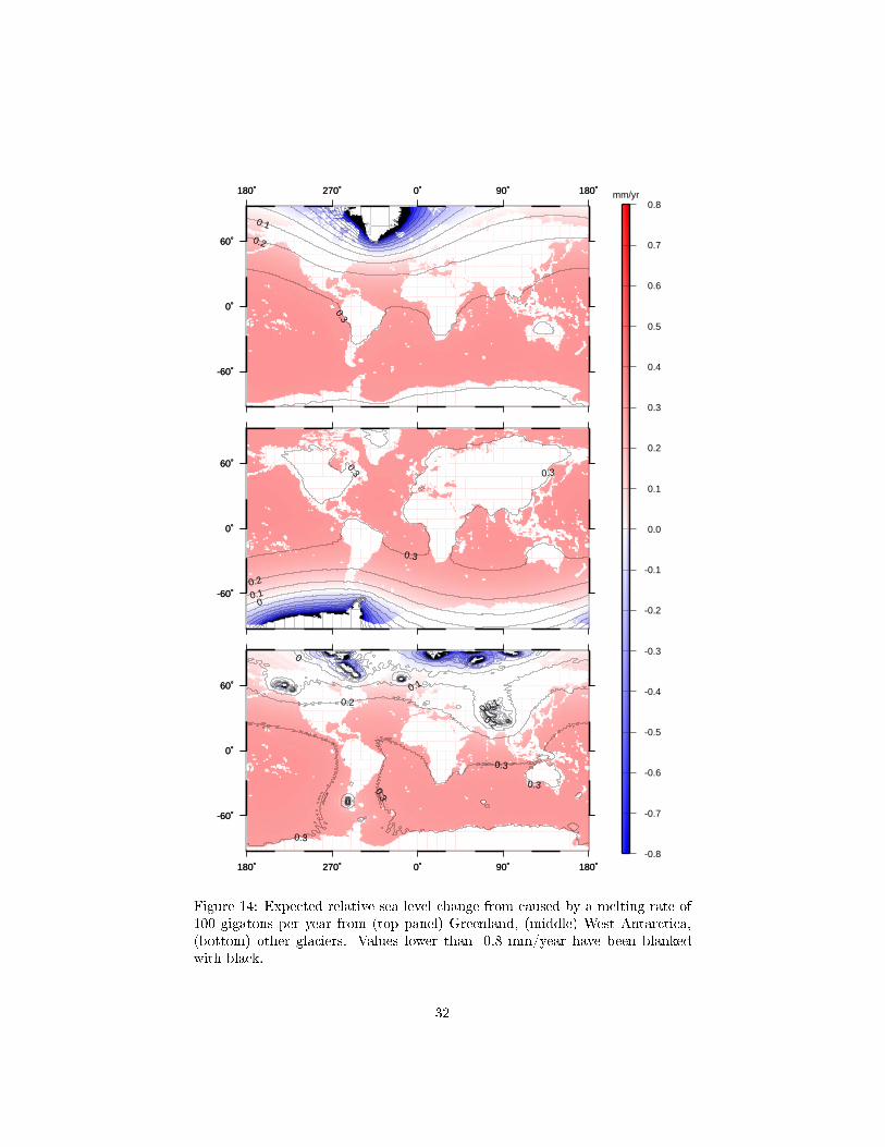
180˚ 270˚ 0˚ 90˚ 180˚
-60˚
0˚
60˚
180˚ 270˚ 0˚ 90˚ 180˚
-60˚
0˚
60˚
-0.2-0.1
0
0
0.1
0.2
0.3
0.3
0.3
0.3
-60˚
0˚
60˚
-60˚
0˚
60˚
00.10.2
0.3
0.3
0.3
180˚ 270˚ 0˚ 90˚ 180˚
-60˚
0˚
60˚
180˚ 270˚ 0˚ 90˚ 180˚
-60˚
0˚
60˚
0.1
0.2
0.3
-0.8
-0.7
-0.6
-0.5
-0.4
-0.3
-0.2
-0.1
0.0
0.1
0.2
0.3
0.4
0.5
0.6
0.7
0.8mm/yr
Figure 14: Expected relative sea level change from caused by a melting rate of100 gigatons per year from (top panel) Greenland, (middle) West Antarctica,(bottom) other glaciers. Values lower than -0.8 mm/year have been blankedwith black.
32

• The purpose of empirical models is to compile observations and �lter outerrors. They will continue to be important for geodetic purposes as wellfor constraining GIA models. Development of empirical models shouldtherefore continue, parallel to geophysical GIA modelling e�orts, as theobservational databases develop.
We end this dissertation with an outlook on a possible application, not primarilyfor geodetic or geophysical purposes, of the theory used in this dissertation.
Lantmäteriet has been commissioned by the government to develop a na-tional digital elevation model, based on laser scanning of the whole country,to meet the need of good elevation data for climate adaptation of the society.Another important step in the climate adaptation work is to try to understand,and predict, how sea levels will respond to potential global warming and melt-ing of continental ice sheets. In Fennoscandia, the relative sea level change isin general negative due to the land uplift. Will this relative sea level fall beexceeded by a potential climate-induced sea level rise?
The sea level equation, as implemented in Paper III and Paper IV, is a suit-able tool to predict how melt water is distributed over the ocean. An exampleof this given in Figure 14 which illustrate the spatial variability of the relativesea level change induced by three di�erent melting scenarios. From the top, thethree panels show the predicted rate of change of sea level from a 100 Gton/yearmelting rate from the Greenland ice sheet, the West Antarctica ice sheet andother continental ice sheets, respectively. Notably is that melting of the Green-land ice sheet does not a�ect sea level in Fennoscandia signi�cantly (the zeroisoline goes right through Sweden) and that the largest impact comes from theWest Antarctica ice sheet. This kind of predictions should be regarded in futureclimate adaptation work.
33

34

References
J. Ågren and R. Svensson. Postglacial land uplift model and system de�nition forthe new Swedish height system RH 2000. LMV-Rapport 2007:4, Lantmäteriet,the Swedish mapping, cadastral and land registration authority, 2007.
Z. Altamimi, X. Collilieux, J. Legrand, B. Garayt, and C. Boucher. ITRF2005:A new release of the international terrestrial reference frame based on timeseries of station positions and earth orientation parameters. J. Geophys. Res.,112:B09401, 2007.
V.R. Barletta and A. Bordoni. E�ect of di�erent implementations of the sameice history in GIA modeling. Journal of Geodynamics, 71(0):65 � 73, 2013.
A.F. Bennett. Inverse Modeling of the Ocean and Atmosphere. Cambridge Univ.Press, Cambridge, U. K., 2002.
L.M. Cathles. The viscosity of the Earth's mantle. Princeton University Press,1975.
A.M. Dziewonski and D.L. Anderson. Preliminary reference earth model.Physics of the Earth and Planetary Interiors, 25:297�356, 1981.
M. Ekman. A concise history of the postglacial land uplift research (from itsbeginning to 1959). Terra Nova, 3:358�365, 1991.
M. Ekman. A consistent map of the postglacial uplift of Fennoscandia. TerraNova, 8:158�165, 1996.
M. Ekman. The world's longest sea level series and a winter oscillation indexfor northern Europe 1774 - 2000. Small Publications in Historical Geophysics,12:1�31, 2003.
M. Ekman. The changing level of the Baltic Sea during 300 years: A clue tounderstanding the Earth. Summer Institute for Historical Geophysics, 2009.
M. Ekman and J. Mäkinen. Recent postglacial rebound, gravity change andmantle �ow in Fennoscandia. Geophysical Journal International, 126:229�234, 1996.
W.E. Farrell. Deformation of the Earth by surface loads. Reviews of Geophysicsand Space Physics, 10(3):761�797, 1972.
W.E. Farrell and J.A. Clark. On postglacial sea level. Geophys. J. R. astr. Soc.,46:467�667, 1976.
O. Gitlein. Absolutgravimetrische Bestimmung der Fennoskandischen Landhe-bung mit dem FG5-220. PhD thesis, Leibniz Universität Hannover, 2009.
35

O. Gitlein and L. Timmen. Atmospheric mass �ow reduction for terrestrialabsolute gravimetry in the Fennoscandian land uplift network. In P. Tregoningand C. Rizos, editors, Dynamic Planet, IAG symposium, Cairns, Australia,22-26 Aug. 2005, volume 130, pages p. 461�466. International Association ofGeodesy, Springer, 2007.
S. Gregersen, P. Voss, and The TORWorking Group. Summary of project TOR:delineation of a stepwise, sharp, deep lithosphere transition across Germany-Denmark-Sweden. Tectonophysics, 360:61�73, 2002.
N.A. Haskell. The motion of a viscous �uid under a surface load. Physics, 6:265�269, 1935.
E.M. Hill, J.L. Davis, M.E. Tamisiea, and M. Lidberg. Combination of geodeticobservations and models for glacial isostatic adjustment �elds in Fennoscan-dia. Journal of Geophysical Research, 115(B07403), 2010.
T. Jamison. On the history of the last geological changes in Scotland. QuartleryJournal of the Geological Society of London, 21:161�203, 1865.
T. Janik, E. Kozlovskaya, P. Heikkinen, J. Yliniemi, and H. Silvennoinen. Evi-dence for preservation of crustal root beneath the Proterozoic Lapland-Kolaorogen (northern Fennoscandian shield) derived from P and S wave velocitymodels of POLAR and HUKKA wide-angle re�ection and refraction pro�lesand FIRE4 re�ection transect. J. Geophys. Res., 114:B06308, 2009.
J.M. Johansson, J.L. Davis, H.-G. Scherneck, G.A. Milne, M. Vermeer, J.X.Mitrovica, R.A. Bennett, B. Jonsson, G. Elgered, P. Elosegui, H. Koivola,M. Poutanen, B.O. Rönnäng, and I.I. Shapiro. Continous GPS measurementsof postglacial adjustment in Fennoscandia 1. Geodetic results. Journal ofGeophysical Research, 107(B8), 2002.
R.A. Kendall, J.X. Mitrovica, and G.A. Milne. On post-glacial sea level -II. Nu-merical formulation and comparative results on spherically symmetric models.Geophys. J. Int., 161:679�706, 2005.
A. Kiviniemi. High precision measurements for studying the secular variationin gravity in Finland. Publ. Finn. Geodet. Inst., 78:64p., 1974.
E. Kozlovskaya, G. Kosarev, I. Aleshin, O. Riznichenko, and I. Sanina. Structureand composition of the crust and upper mantle of the Archean-Proterozoicboundary in the Fennoscandian shield obtained by joint inversion of receiverfunction and surface wave phase velocity of recording of the SVEKALAPKOarray. Geophys. J. Int., 175:135�152, 2008.
K. Lambeck, C. Smither, and P. Johnston. Sea-level change, glacial rebound andmantle viscosity for northern Europe. Geophys. J. Int., 134:102�144, 1998.
36

Lantmäteriet. Geodesy 2010 - A strategic plan for Lantmäteriet'sgeodetic activities 2011 - 2020. http://www.lantmateriet.se/en/
Maps-and-geographic-information/GPS-and-geodetic-surveys/
Geodesy/, 2011. Can be downloaded from Lantmäteriets homepage;accessed 27-August-2013.
M. Lidberg, J.M. Johansson, H.-G. Scherneck, and J.L. Davis. An improvedand extended GPS derived velocity �eld for the glacial isostatic adjustmentin Fennoscandia. Journal of Geodesy, 81(3):213�230, 2007.
M. Lidberg, J.M. Johansson, H.-G. Scherneck, G.A. Milne, and J.L. Davis. Newresults based on reprocessing of 13 years continous GPS of the FennoscandiaGIA process from BIFROST. In M.G. Sideris, editor, Proceedings of the 2007IAG general Assembly, Perugia Italy, July 2-13, volume 133, page p. 557�.International Association of Geodesy, Springer, 2008.
M. Lidberg, J.M. Johansson, H.-G. Scherneck, and G. A. Milne. Recent resultsbased on continuous GPS observations of the GIA process in Fennoscandiafrom BIFROST. Journal of Geodynamics, 50:8�18, 2010.
I.M. Longman. A Green's function for determining the deformation of the Earthunder surface mass loads. 1. Theory. Journal of Geophysical Research, 67(2):845�850, 1962.
I.M. Longman. A Green's function for determining the deformation of the earthunder surface mass loads. 2. computations and numerical results. Journal ofGeophysical Research, 68:485�496, 1963.
J. Mäkinen and V. Saaranen. Determination of post-glacial land uplift fromthree precise levellings in Finland. Journal of Geodesy, 72:516�529, 1998.
J. Mäkinen, M. Ekman, Å. Midtsundstad, and O. Remmer. The Fennoscandianland uplift gravity lines 1966 - 1984. Rep. Finn. Geod. Inst., 85:4:238 p., 1986.
J. Mäkinen, A. Engfeldt, B.G. Harsson, H. Ruotsalainen, G. Stykowski, T. Oja,and D. Wolf. The Fennoscandian land uplift gravity lines 1966-2004. InChristopher Jekeli, Luisa Bastos, and Joana Fernandes, editors, Gravity,Geoid and Space Missions, volume 129 of International Association of GeodesySymposia, pages 328�332. Springer Berlin Heidelberg, 2005.
J. Mäkinen, A. Engfeldt, O. Gitlein, B.G. Harsson, J. Kaminskis, F. Klop-ping, T. Oja, E. Parseliunas, B.R. Pettersen, H. Ruotsalainen, G. Stykowski,H. Wilmes, and D. Wolf. Repeated absolute and relative gravity measure-ments in Fennoscandian postglacial rebound area: comparison of gravitychange with observed vertical motion and with GIA models. Poster at EGUGeneral Assenbly, Vienna, May 2-7, 2010, 2010.
Z. Martinec. Spectral-�nite element approach for three-dimensional viscoelasticrelaxation in a spherical earth. Geophys. J. Int., 142:117�141, 2000.
37

S. Mazzotti, A. Lambert, J. Henton, T.S. James, and N. Courtier. Absolutegravity calibration of GPS velocitites and glacial isostatic adjustment in mid-continent North America. Geophysical Research Letters, 30:L24311, 2011.
A. Memin, J. Hinderer, and Y. Rogister. Separation of the geodetic consequencesof past and present ice-mass change: In�uence of topography with applicationto Svalbard (Norway). Pure and Applied Geophysics, 169:1357�1372, 2012.
G.A. Milne, J.L. Davis, J.X. Mitrovica, H.-G. Scherneck, J.M. Johansson,M. Vermeer, and H. Koivula. Space-geodetic constraints on glacial isostaticadjustment in Fennoscandia. Science, 291(2381-2385), 2001.
G.A. Milne, J.X. Mitrovica, H.-G. Scherneck, J.L. Davis, J. M. Johansson,H. Koivula, and M. Vermeer. Continuous GPS measurements of postglacialadjustment in Fennoscandia: 2. Modeling results. Journal of GeophysicalResearch, 109(B02412), 2004.
J.X. Mitrovica and G.A. Milne. On post-glacial sea level: I. General theory.Geophys. J. Int., 154:253�267, 2003.
J.X. Mitrovica, M.E. Tamisiea, J.L. Davis, and G.A. Milne. Recent mass balanceof polar ice sheets inferred from patterns of global sea-level change. Nature,409:1026�1029, 2001.
H. Moritz. Advanced Physical Geodesy. H. Wichmann, Karlsruhe, Germany.,1980.
J. Müller, M. Naeimi, O. Gitlein, L. Timmen, and H. Denker. A land upliftmodel in Fennoscandia combining GRACE and absolute gravimetry data.Physics and Chemistry of the Earth, 53-54:54�60, 2012.
M. Naujoks, C. Kroner, A. Weise, T. Jahr, P. Krause, and S. Eisner. Eval-uating local hydrological modelling by temporal gravity observations and agravimetric three-dimensional model. Geophys. J. Int., 182(1):233�249, 2010.
J. Neumeyer, F. Barthelmes, O. Dierks, F. Flechtner, M. Harnisch, G. Harnisch,J. Hinderer, Y. Imanishi, C. Kroner, B. Meurers, S. Petrovic, Ch. Reigber,R. Schmidt, P. Schwintzer, H.-P. Sun, and H. Virtanen. Combination oftemporal gravity variations resulting from superconducting gravimeter (SG)recordings, GRACE satellite observations and global hydrology models. Jour-nal of Geodesy, 79(10-11):573�585, 2006.
T.M. Niebauer, G.S. Sasagawa, J.E. Faller, R. Hilt, and F. Klopping. A newgeneration of absolute gravimeters. Metrologia, 32:159�180, 1995.
J. E. Nielsen. Absolute gravimetry - for monitoring climate change and geody-namics in Greenland. PhD thesis, National Space Institute, Technical Uni-versity of Denmark, Kgs. Lyngby, Denmark, 2013.
38
P.-A. Olsson. Contribution to the modelling of postglacial gravity change inFennoscandia. Licentiate thesis, Chalmers University of Technology, Gothen-burg, 2011.
P.-A. Olsson and M. Ekman. Crustal loading and gravity change during thegreatest storm �ood in the Baltic Sea. Small Publications in Historical Geo-physics, 19:1�10, 2009.
W.R. Peltier. The impulse response of a Maxwell Earth. Reviews of Geophysicsand Space Physics, 12(4):649�669, 1974.
W.R. Peltier. Glacial-isostatic adjustment - II. The inverse problem. GeophysicalJournal of the Royal Astronomical Society, 46:669�705, 1976.
W.R. Peltier. The LAGEOS constraint on deep mantle viscosity: Results from anew normal mode method for the inversion of viscoelastic relaxation spectra.Journal of Geophysical Research, 90(B11):9411�9421, 1985.
W.R. Peltier. Ice age paleotopgraphy. Science, 265(5169):195�201, 1994.
W.R. Peltier. Mantle viscosity and ice-age ice sheet topography. Science, 273(5280):1359�1364, 1996.
W.R. Peltier. Global glacial isostasy and the surface of the ice-age Earth: TheICE-5G (VM2) model and GRACE. Annu. Rev. Earth. Planet. Sci., 32:111�149, 2004.
W.R. Peltier and J.T. Andrews. Glacial-isostatic adjustment - I. The forwardproblem. Geophysical Journal of the Royal Astronomical Society, 46(3):605�646, 1976.
R. Sabadini and L.L.A. Vermeersen. Global Dynamics of the Earth. Applicationsof Normal Mode Relaxation Theory to Solid-Earth Geophysics, volume 20 ofModern approaches in geophysics. Kluwer Academic Publisher, 2004.
R. Sabadini, D.A. Yuen, and M. Portney. The e�ects of upper mantle lateralheterogeneities on postglacial rebound. Geophys. Res. Lett., 13(4):337�340,1986.
M. Sacher, J. Ihde, G. Liebsch, and J. Mäkinen. EVRF2007 as realization ofthe European vertical reference system. http://www.euref.eu, 2008. Pre-sented at the Symposium of the IAG Sub-commission for Europe (EUREF)in Brussels, June 18-21, 2008. Submitted to the proceedings. From EUREFhome page; accessed 5-May-2011.
H.-G. Scherneck, J.M. Johansson, G. Elgered, J.L. Davis, B. Jonsson,G. Hedling, H. Koivula, M. Ollikainen, M. Poutanen, M. Vermeer, J.X. Mitro-vica, and G.A. Milne. BIFROST: Observing the three-dimensional deforma-tion of Fennoscandia. In Jerry X. Mitrovica and Bert L. A. Vermeersen,editors, Ice Sheets, Sea Level and the Dynamic Earth, Geodynamic Series 29,pages 69�93. American Geophysical Union, 2002.
39

H.-G. Scherneck, M. Lidberg, R. Haas, J.M. Johansson, and G.A. Milne.BIFROST project: Contemporary strain rates in Fennoscandia from elevenyears of continous GPS. Journal of Geodynamics, 50:19�26, 2010.
P. Schmidt. Glacial Isostatic Adjustment. Inferences on properties and pro-cesses in the upper mantle from 3D dynamical modeling. PhD thesis, UppsalaUniversity, Uppsala, Sweden, 2004.
SKB. Climate and climate-related issues for the safety assessment SR-site.Technical Report TR-10-49, Svensk kärnbränselhantering AB, 2010.
G. Spada, V.R. Barletta, V. Klemann, R.E.M. Riva, Z. Martinec, P. Gasperini,B. Lund, D. Wolf, L.L.A. Vermeersen, and M.A. King. A benchmark studyfor glacial isostatic adjustment codes. Geophysical Journal International, 185:106�132, 2011.
H. Ste�en and P. Wu. Glacial isostatic adjustment in Fennoscandia - a reviewof data and modeling. Journal of geodynamics, 52:169�204, 2011.
H. Ste�en, P. Wu, and H. Wang. Determination of the Earth's structure inFennoscandia from GRACE and implications for the optimal post-processingof GRACE data. Geophys. J. Int., 182:1295�1310, 2010.
H. Ste�en, P. Wu, and H. Wang. Optimal locations for absolute gravity mea-surements and sensitivity of GRACE observations for constraining glacialisostatic adjustment on the northern hemisphere. Geophys. J. Int., 190:1483�1494, 2012.
L. Timmen, O. Gitlein, V. Klemann, and D. Wolf. Observing gravity change inthe Fennoscandian uplift area with the Hanover absolute gravimeter. Pureand Applied Geophysics, 169:1331�1342, 2012.
A.M. Tushingham and W.R. Peltier. Ice-3G: A new global model of late pleis-tocene deglaciation based upon geophysical predictions of post-glacial relativesea level change. Journal of Geophysical Research, 96(B3):4497�4523, 1991.
M. Van Camp, S. D. P. Williams, and O. Francis. Uncertainty of absolutegravity measurements. Journal of Geophysical Research, 110(B05406), 2005.
M. Van Camp, M. Vanclooster, O. Crommen, T. Petermans, K. Verbeeck,B. Meurers, T. van Dam, and A. Dassargues. Hydrogeological investigationsat the Membach station, Belgium, and application to correct long periodicgravity variation. Journal of Geophysical Research, 111(B10403), 2006.
M. Van Camp, L. Metivier, O. de Viron, B. Meurers, and S.D.P. Williams.Characterizing long-time scale hydrological e�ects on gravity for improveddistinction of tectonic signals. Journal of Geophysical Research, 115(B07407),2010.
40
F.A. Vening Meinesz. Gravity and the hypothesis of convection-currents in theEarth. Koninklijke Akademie van Wetenschappen te Amsterdam, 37:37�45,1934.
O. Vestøl. Determination of postglacial land uplift in Fennoscandia from level-ing, tide-gauges and continuous GPS stations using least squares collocation.Journal of Geodesy, 80:248�258, 2006.
H. Virtanen. Loading e�ects in metsähovi from the atmosphere and the Balticsea. Journal of Geodynamics, 38(407-422), 2004.
H. Virtanen. Studies of Earth Dynamics with the Superconducting Gravimeter.PhD thesis, University of Helsinki, 2006.
J. Wahr, H. DaZhong, and A. Trupin. Predictions of vertical uplift caused bychanging polar ice volumes on a viscoelastic earth. Geophys. Res. Lett., 22(8):977�980, 1995.
H.S. Wang, P. Wu, and W. van der Wal. Using postglacial sea level, crustal ve-locities and gravity-rate-of-change to constrain the in�uence of thermal e�ectson mantle lateral heterogeneities. J. Geodyn., 46(3-5):104�117, 2008.
P. Whitehouse. Glacial isostatic adjustment and sea-level change. State of theart report. Technical Report TR-09-11, Swedish Nuclear Fuel and WasteManagement Co, 2009.
P. Wu. Response of a Maxwell Earth to applied surface mass loads:GlacialIsostatic Adjustment. Master's thesis, Department of Physics, University ofToronto, 1978.
P. Wu. Using commercial �nite element packages for the study of earth defor-mations, sea levels and the state of stress. Geophys. J. Int., 158(2):401�408,2004.
P. Wu and W.R. Peltier. Viscous gravitational relaxation. Geophys. J. R. astr.Soc., 70:435�485, 1982.
P. Wu and W.R. Peltier. Glacial isostatic adjustment and the free air gravityanomaly as a constraint on deep mantle viscosity. Geophys. J. R. astr. Soc.,74:377�449, 1983.
P. Wu, H. Ste�en, and H. Wang. Optimal locations for GPS measurements inNorth America and northern Europe for constraining glacial isostatic adjust-ment. Geophys. J. Int., 181(2):653�664, 2010.
41