University of Otago, New Zealand

E-mail: igor@physics.otago.ac.nz

On-line Object Oriented Monte Carlo for the needs of Biophotonics and Biomedical Optics

Igor Meglinski

Method Monte Carlo (MC) • Started 1930 by Enrico Fermi (most famous early use) to calculate

the properties of the newly-discovered neutron. • 1946 Stanislaw Ulam suggested to use random sampling to

simulate path length of neutrons; 1947 developed by John von Newmann.

• 1949 Nick Metropolis and S. Ulam summarized the ideas. • Since 1950s MC is actively used for work relating to the

development of the nuclear/hydrogen bomb, atmospheric optics, geophysics, etc. (Meyer, Sobol, Marchuk; Abubakirov).

• 1980/90s: Noassal, Bonner, Chance, Feng, Kejzer, Prahl, Jacques, Wang, Yaroslavsky, Tuchin, Chernomordik and others are used MC for estimation of fluence rate distribution…

• Nowadays – 1000 papers in various optical diagnostic applications

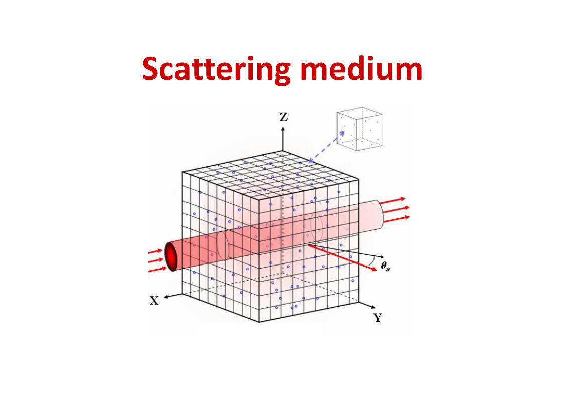
Scattering medium

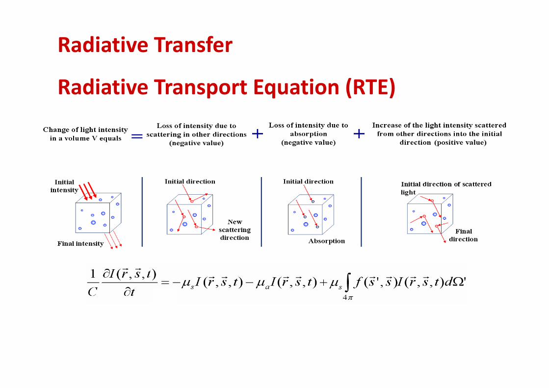
Radiative Transfer

Radiative Transport Equation (RTE)

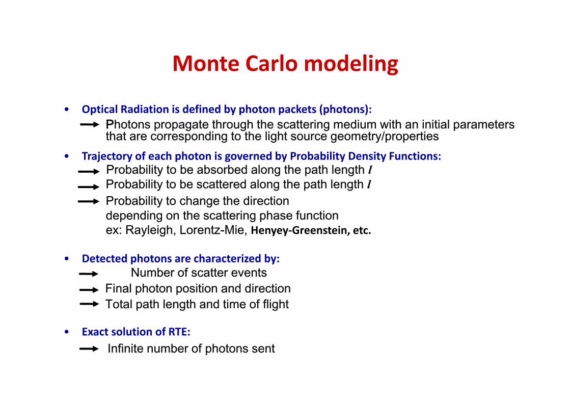
• Optical Radiation is defined by photon packets (photons): • Trajectory of each photon is governed by Probability Density Functions: • Detected photons are characterized by: • Exact solution of RTE:

Monte Carlo modeling

l

l

Henyey-Greenstein, etc.

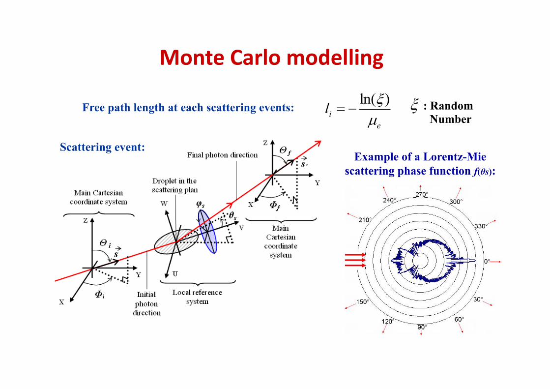
Free path length at each scattering events: e

il �� )ln(

��

Monte Carlo modelling

Scattering event: Example of a Lorentz-Mie

scattering phase function f(θs):

� : Random Number

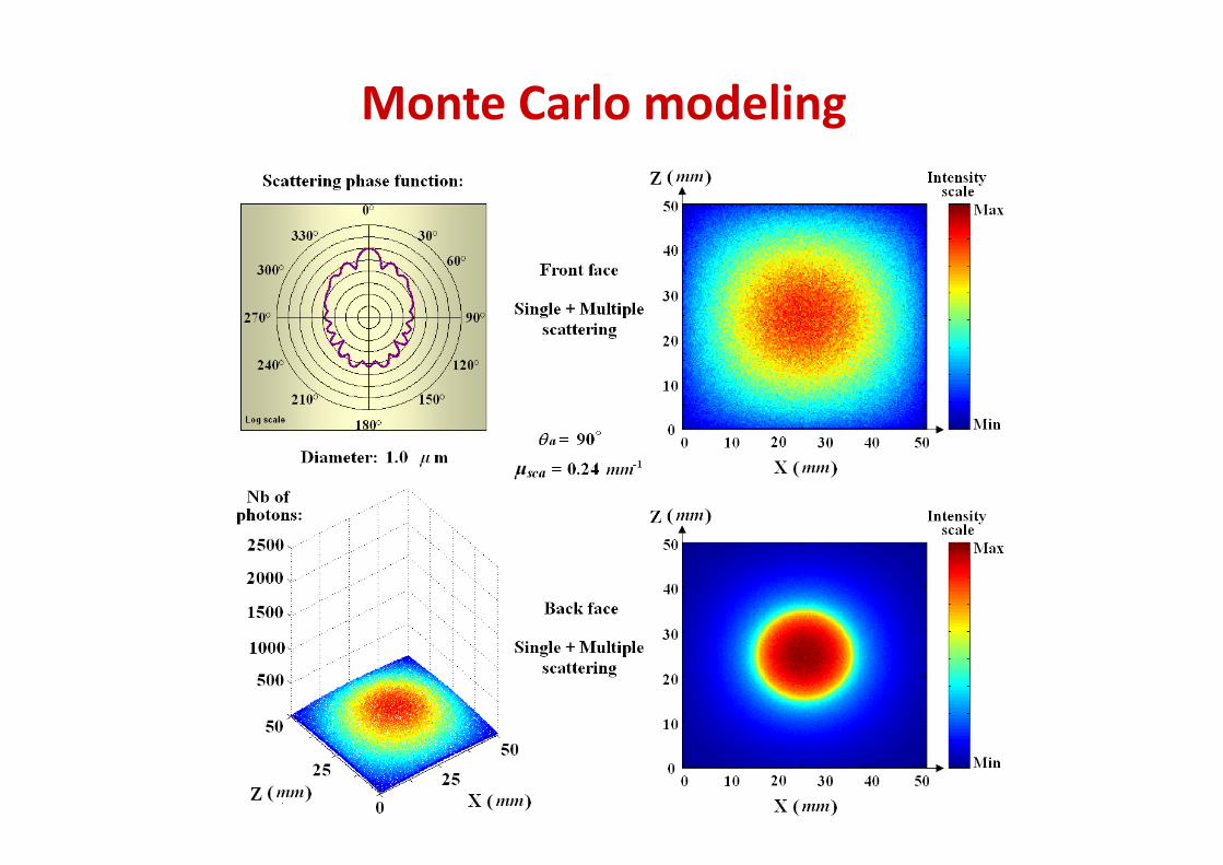
Monte Carlo modeling

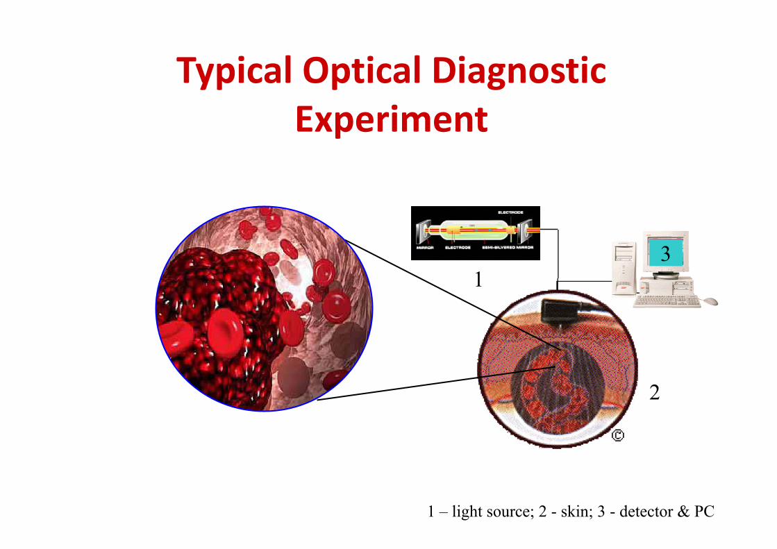
Typical Optical Diagnostic Experiment

1 – light source; 2 - skin; 3 - detector & PC

2

3 1

Probe

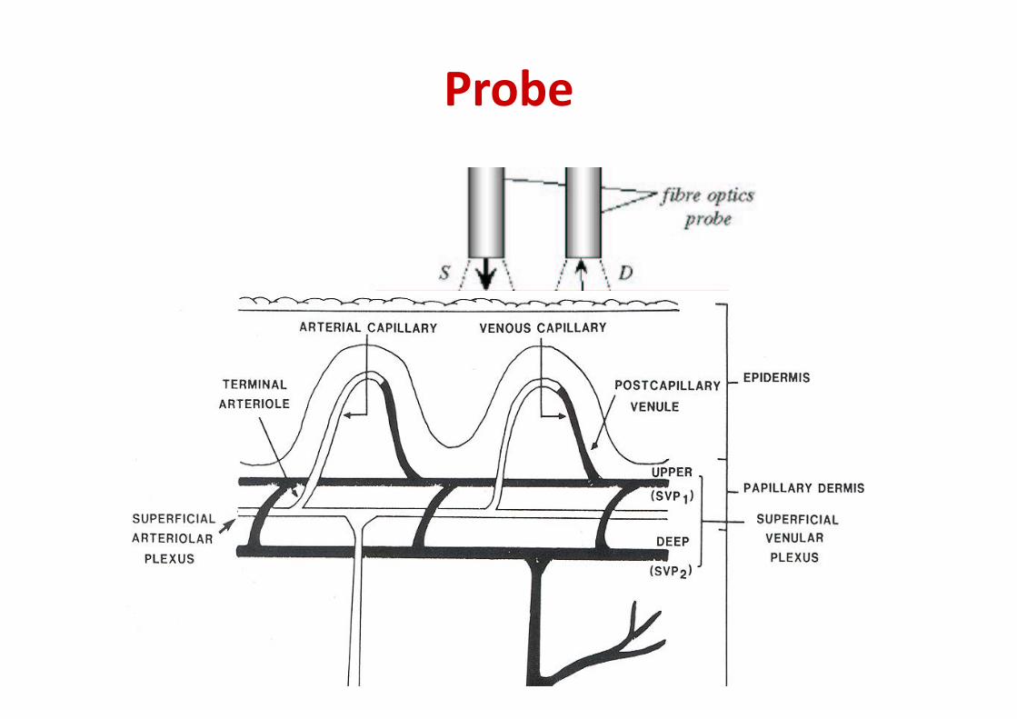
Probe

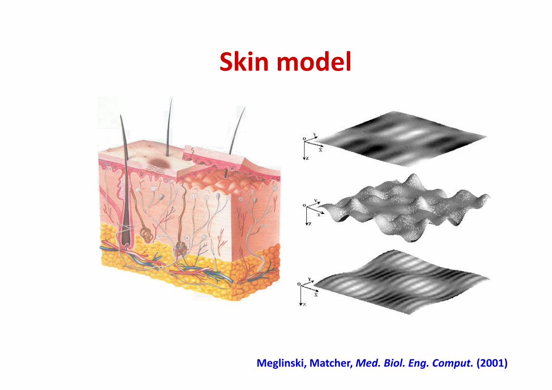
Skin model

Meglinski, Matcher, Med. Biol. Eng. Comput. (2001)

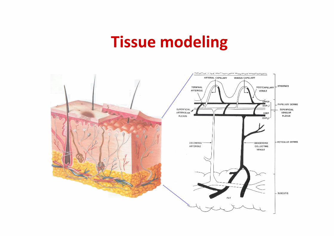
Tissue modeling

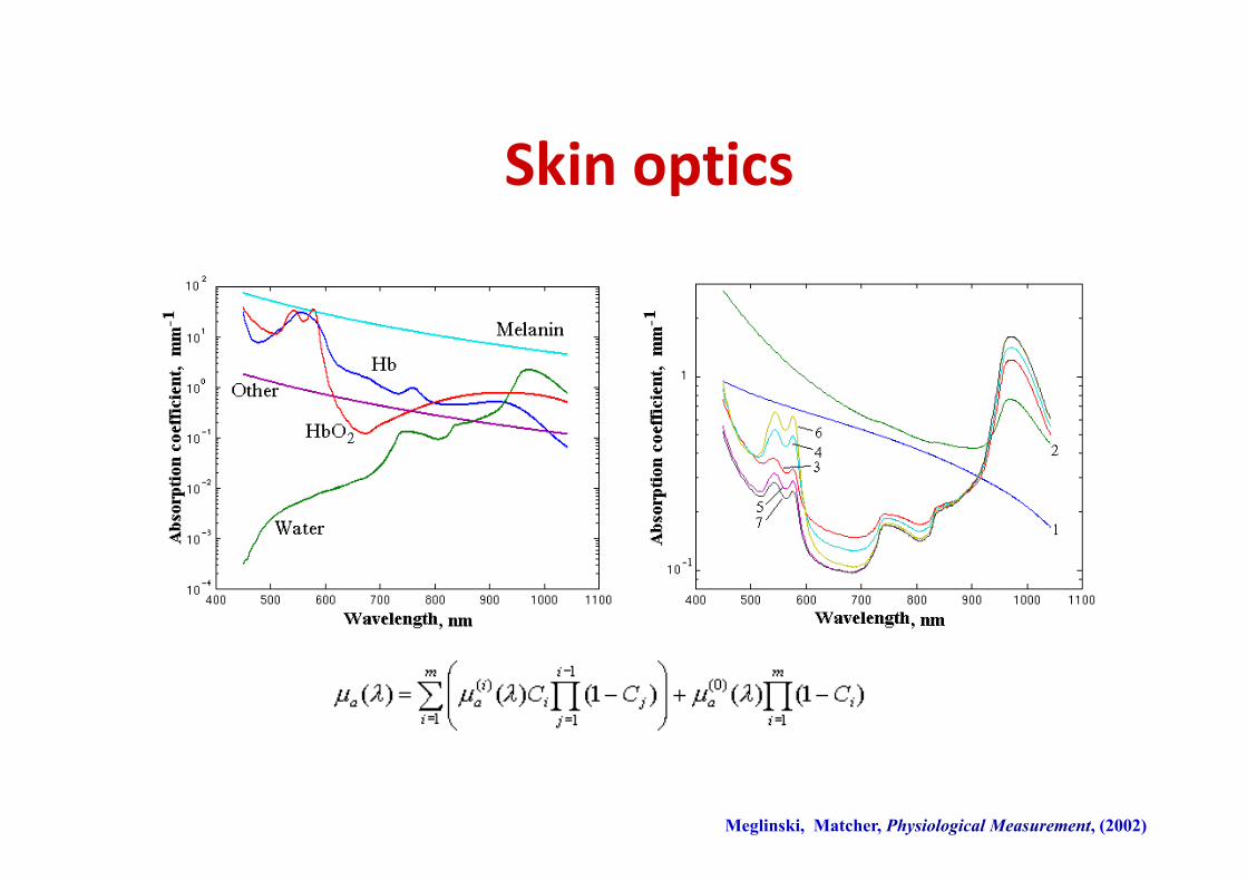
Skin optics

Meglinski, Matcher, Physiological Measurement, (2002)

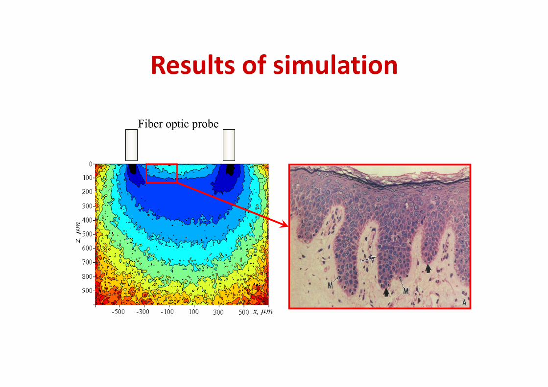
Results of simulation

Fiber optic probe

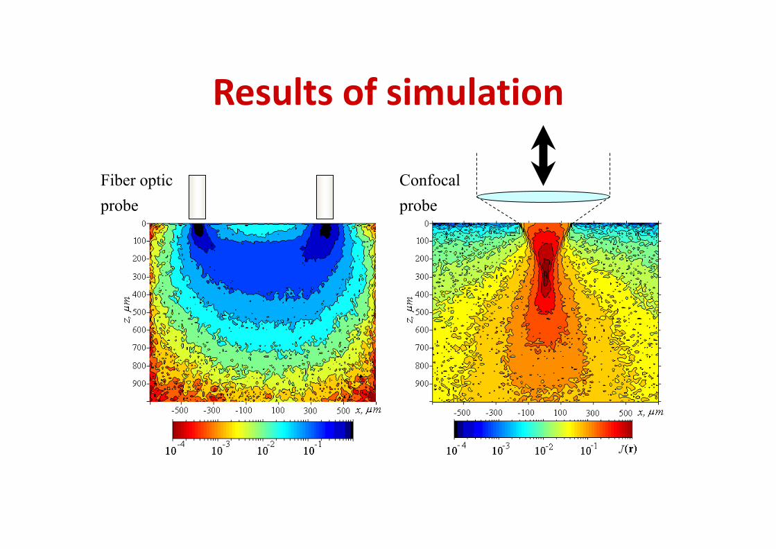
Fiber optic probe

Confocal probe

Results of simulation

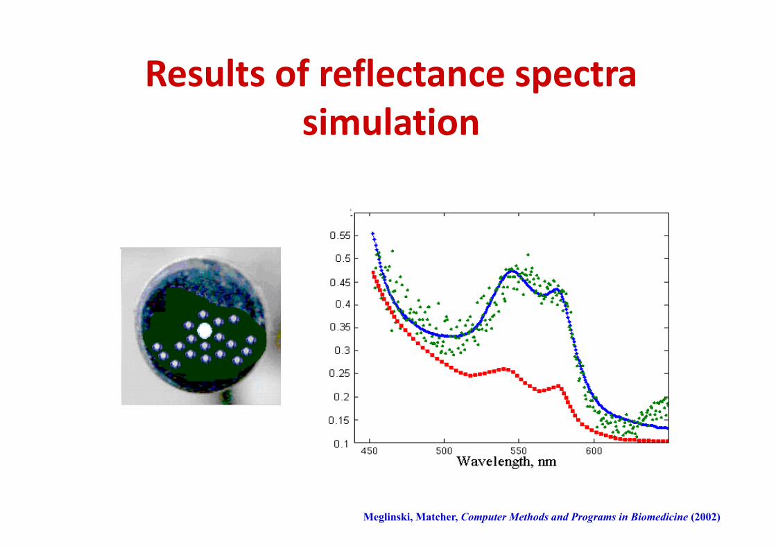
Results of reflectance spectra simulation

Meglinski, Matcher, Computer Methods and Programs in Biomedicine (2002)

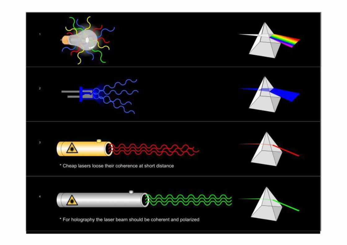
Coherence and Polarisation

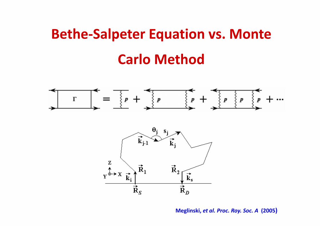
Meglinski, et al. Proc. Roy. Soc. A (2005)

Bethe-Salpeter Equation vs. Monte

Carlo Method

� � � �� � � � � ���

��

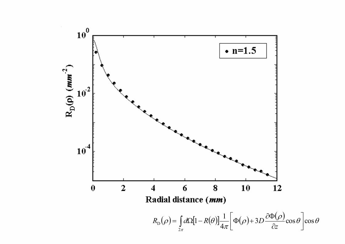
coscos3411

2D �

����

���

����� � zDRdR

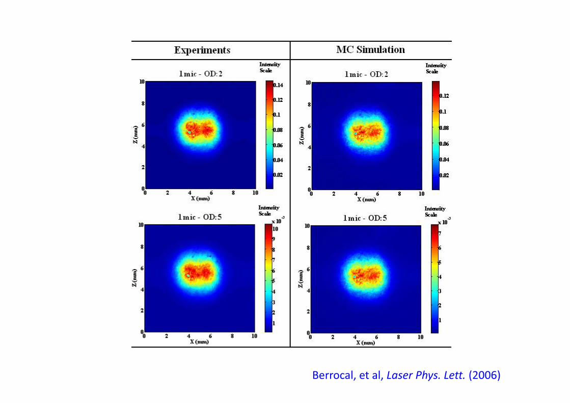
Berrocal, et al, Laser Phys. Lett. (2006)

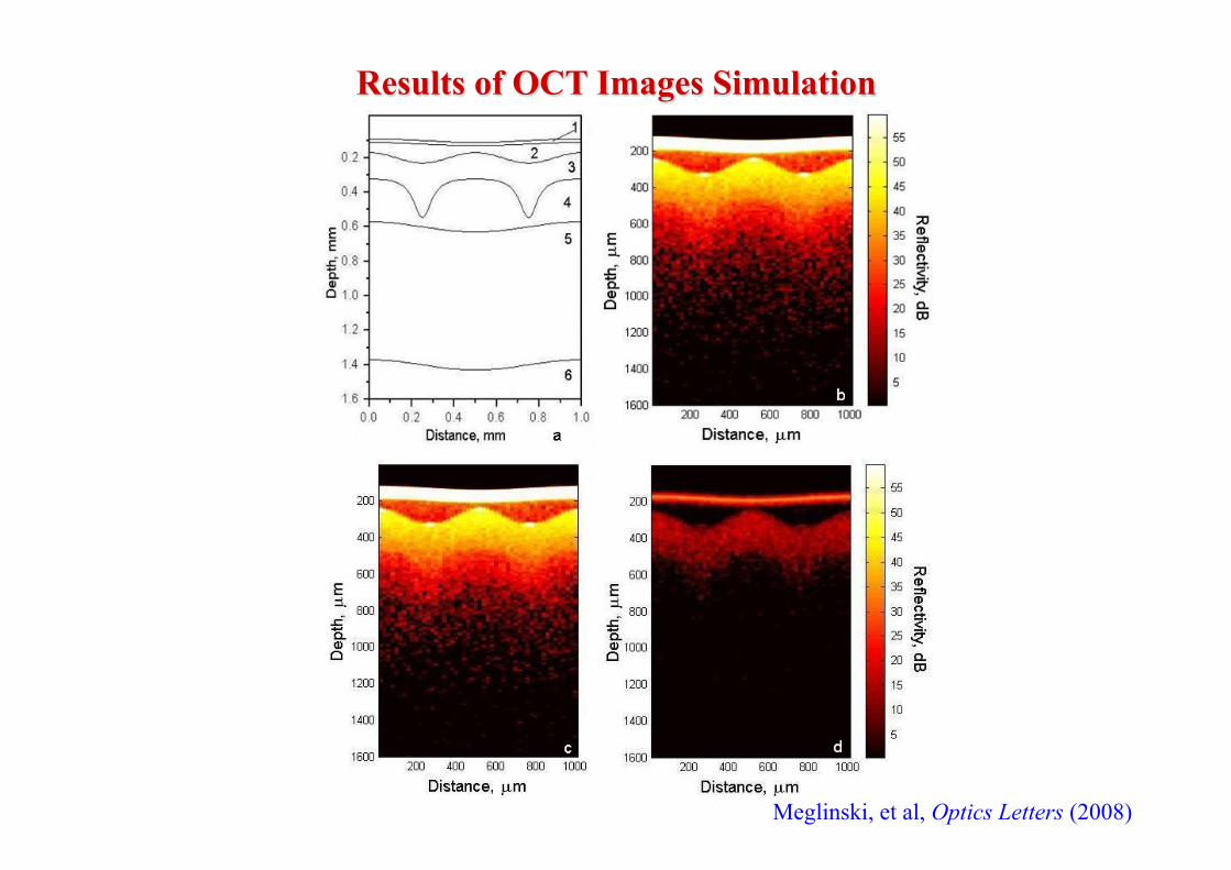
Results of OCT Images Simulation

Meglinski, et al, Optics Letters (2008)

���s, �a � li = - ln(�)/ �s

D S

W0 W

li

Rin

R()

Wi-1

Wi

X

Z

Y

� �� � � ��� ��� ������ ����� ��

2

1

1

10 exp1 �

��

����

��

�

���

��� ��

��

jN

iia

M

pii lRWRW �

Method Monte Carlo

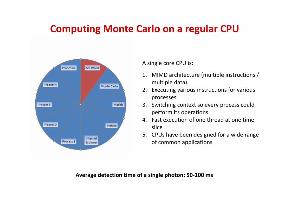
Computing Monte Carlo on a regular CPU

1. MIMD architecture (multiple instructions / multiple data)

2. Executing various instructions for various processes

3. Switching context so every process could perform its operations

4. Fast execution of one thread at one time slice

5. CPUs have been designed for a wide range of common applications

Average detection time of a single photon: 50-100 ms

A single core CPU is:

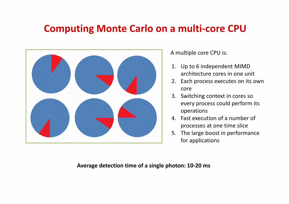
Computing Monte Carlo on a multi-core CPU

Average detection time of a single photon: 10-20 ms

1. Up to 6 independent MIMD architecture cores in one unit

2. Each process executes on its own core

3. Switching context in cores so every process could perform its operations

4. Fast execution of a number of processes at one time slice

5. The large boost in performance for applications

A multiple core CPU is:

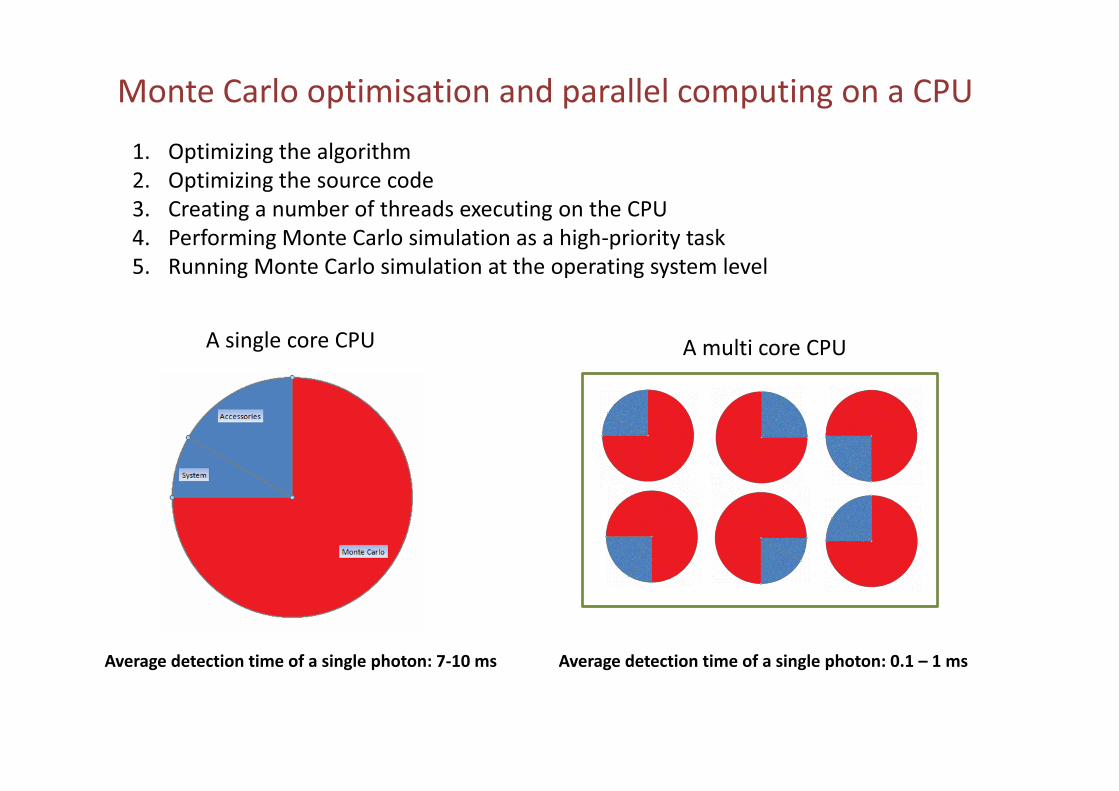
Monte Carlo optimisation and parallel computing on a CPU

Average detection time of a single photon: 7-10 ms

1. Optimizing the algorithm 2. Optimizing the source code 3. Creating a number of threads executing on the CPU 4. Performing Monte Carlo simulation as a high-priority task 5. Running Monte Carlo simulation at the operating system level

A single core CPU A multi core CPU

Average detection time of a single photon: 0.1 – 1 ms

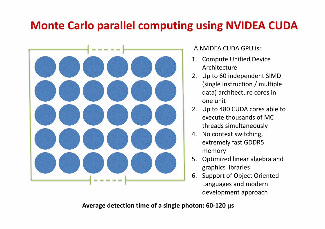
Monte Carlo parallel computing using NVIDEA CUDA

Average detection time of a single photon: 60-120 μs

A NVIDEA CUDA GPU is: 1. Compute Unified Device

Architecture 2. Up to 60 independent SIMD

(single instruction / multiple data) architecture cores in one unit

2. Up to 480 CUDA cores able to execute thousands of MC threads simultaneously

4. No context switching, extremely fast GDDR5 memory

5. Optimized linear algebra and graphics libraries

6. Support of Object Oriented Languages and modern development approach

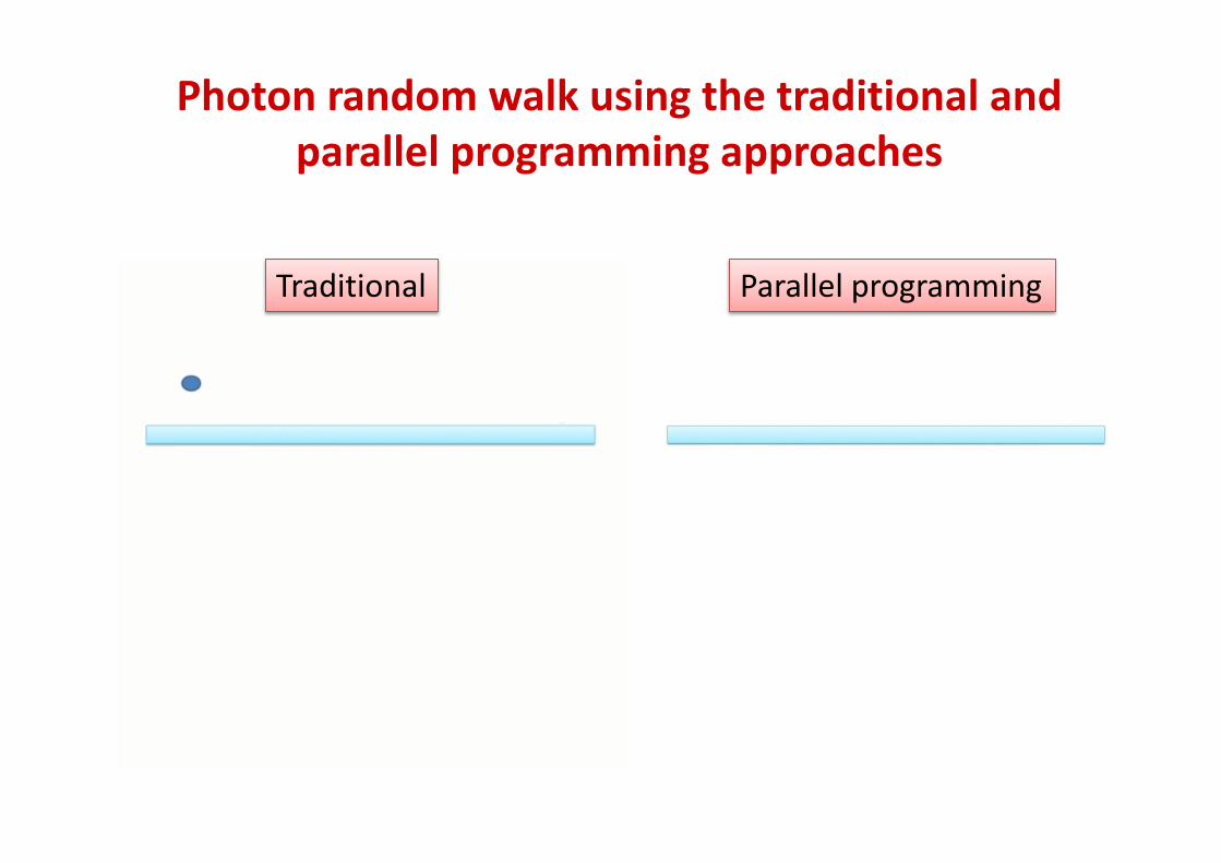
Photon random walk using the traditional and parallel programming approaches

Traditional Parallel programming

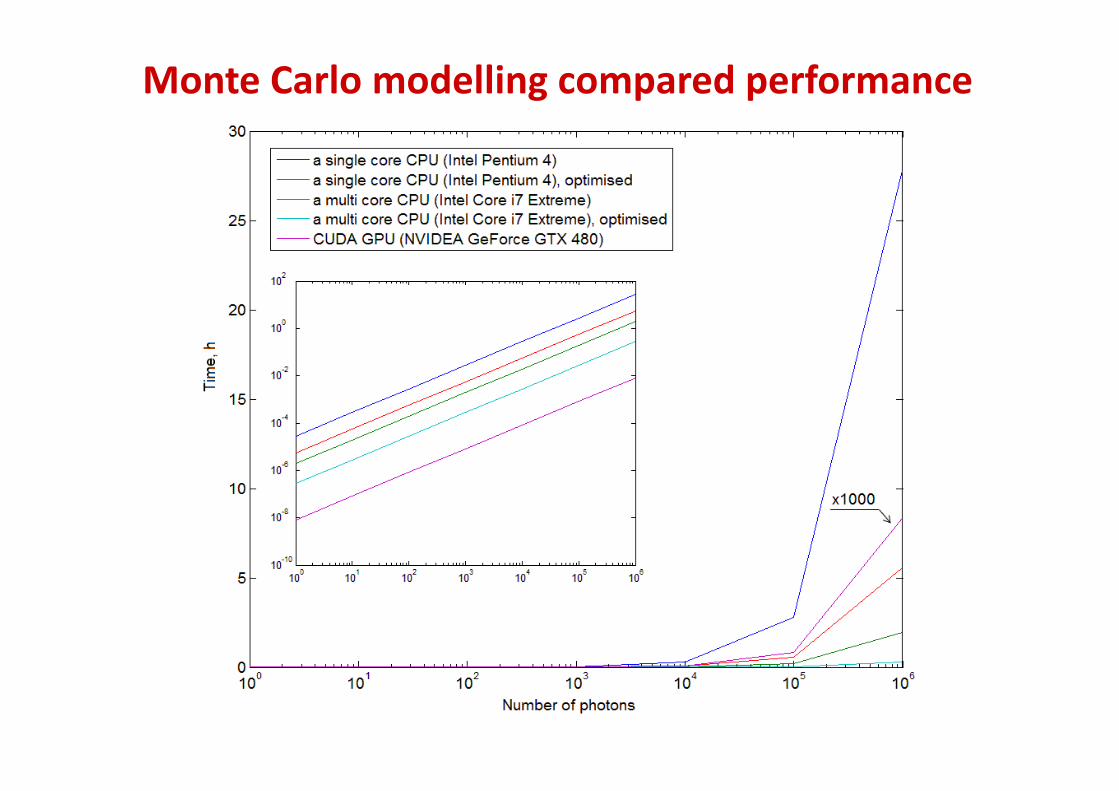
Monte Carlo modelling compared performance

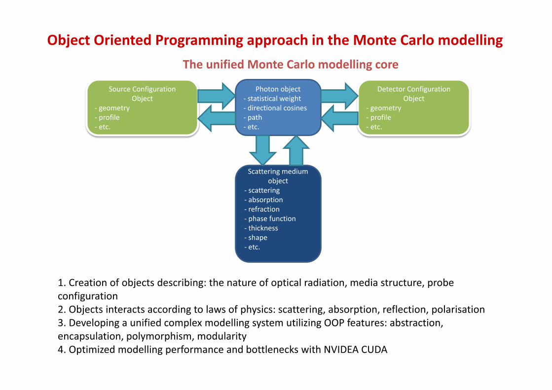
Object Oriented Programming approach in the Monte Carlo modelling

1. Creation of objects describing: the nature of optical radiation, media structure, probe configuration 2. Objects interacts according to laws of physics: scattering, absorption, reflection, polarisation 3. Developing a unified complex modelling system utilizing OOP features: abstraction, encapsulation, polymorphism, modularity 4. Optimized modelling performance and bottlenecks with NVIDEA CUDA

Photon object - statistical weight - directional cosines - path - etc.

Scattering medium object

- scattering - absorption - refraction - phase function- thickness - shape - etc.

Source Configuration Object

- geometry - profile - etc.

Detector Configuration Object

- geometry - profile - etc.

The unified Monte Carlo modelling core

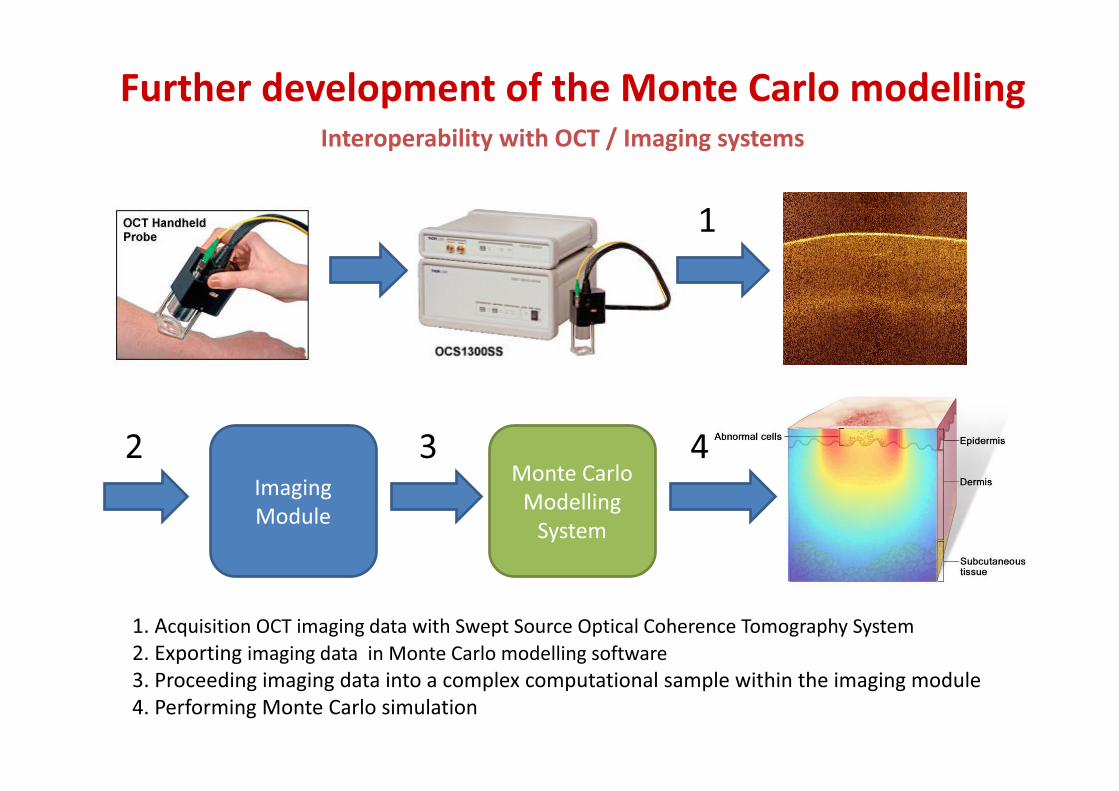
Further development of the Monte Carlo modelling Interoperability with OCT / Imaging systems

Imaging Module

Monte Carlo Modelling

System

1. Acquisition OCT imaging data with Swept Source Optical Coherence Tomography System 2. Exporting imaging data in Monte Carlo modelling software 3. Proceeding imaging data into a complex computational sample within the imaging module 4. Performing Monte Carlo simulation

2 3 4

1

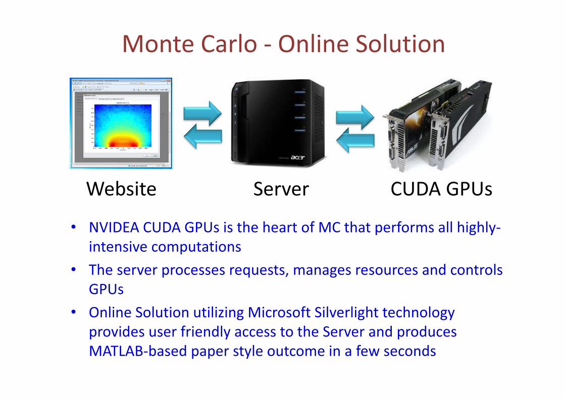
Website Server CUDA GPUs

Monte Carlo - Online Solution

• NVIDEA CUDA GPUs is the heart of MC that performs all highly-intensive computations

• The server processes requests, manages resources and controls GPUs

• Online Solution utilizing Microsoft Silverlight technology provides user friendly access to the Server and produces MATLAB-based paper style outcome in a few seconds

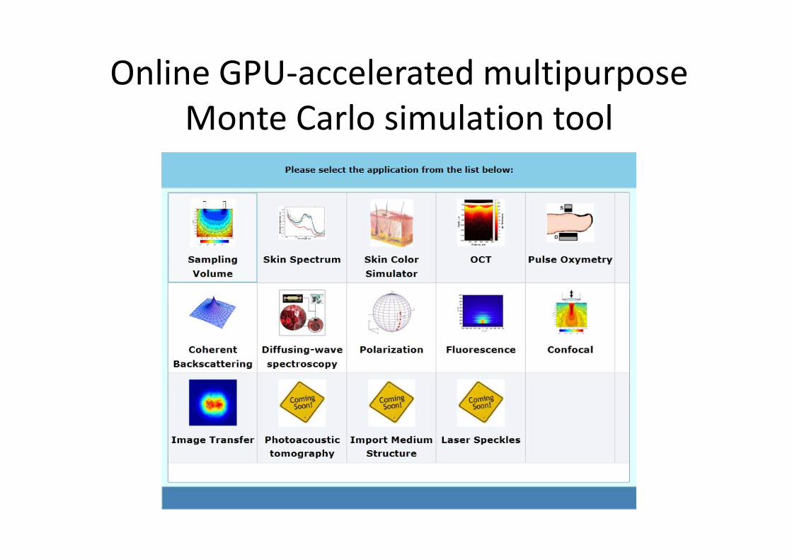
Online GPU-accelerated multipurpose Monte Carlo simulation tool

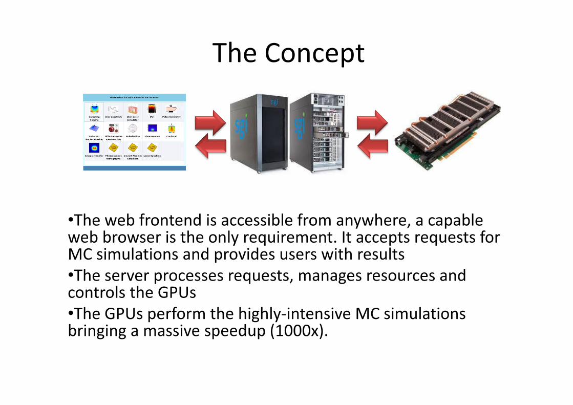
The Concept

•The web frontend is accessible from anywhere, a capable web browser is the only requirement. It accepts requests for MC simulations and provides users with results •The server processes requests, manages resources and controls the GPUs •The GPUs perform the highly-intensive MC simulations bringing a massive speedup (1000x).

Generalized object-oriented MC model structure

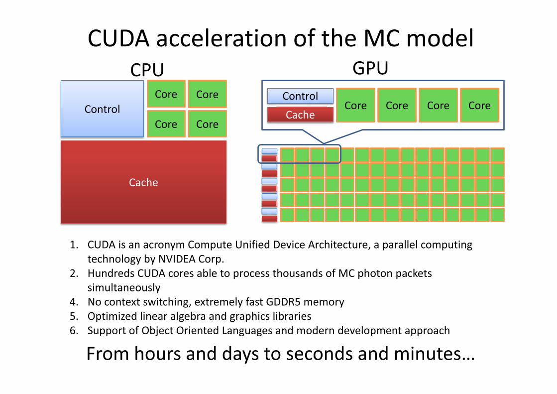
CUDA acceleration of the MC model

Control

Cache

Core Core

Core Core Core

Cache Control

Core Core Core

1. CUDA is an acronym Compute Unified Device Architecture, a parallel computing technology by NVIDEA Corp.

2. Hundreds CUDA cores able to process thousands of MC photon packets simultaneously

4. No context switching, extremely fast GDDR5 memory 5. Optimized linear algebra and graphics libraries 6. Support of Object Oriented Languages and modern development approach

CPU GPU

From hours and days to seconds and minutes…

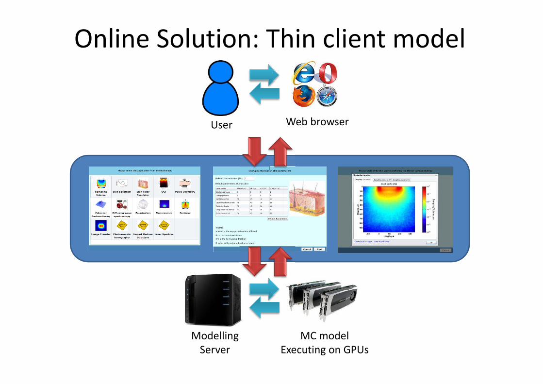
Online Solution: Thin client model

Web browser

Modelling Server

MC model Executing on GPUs

User

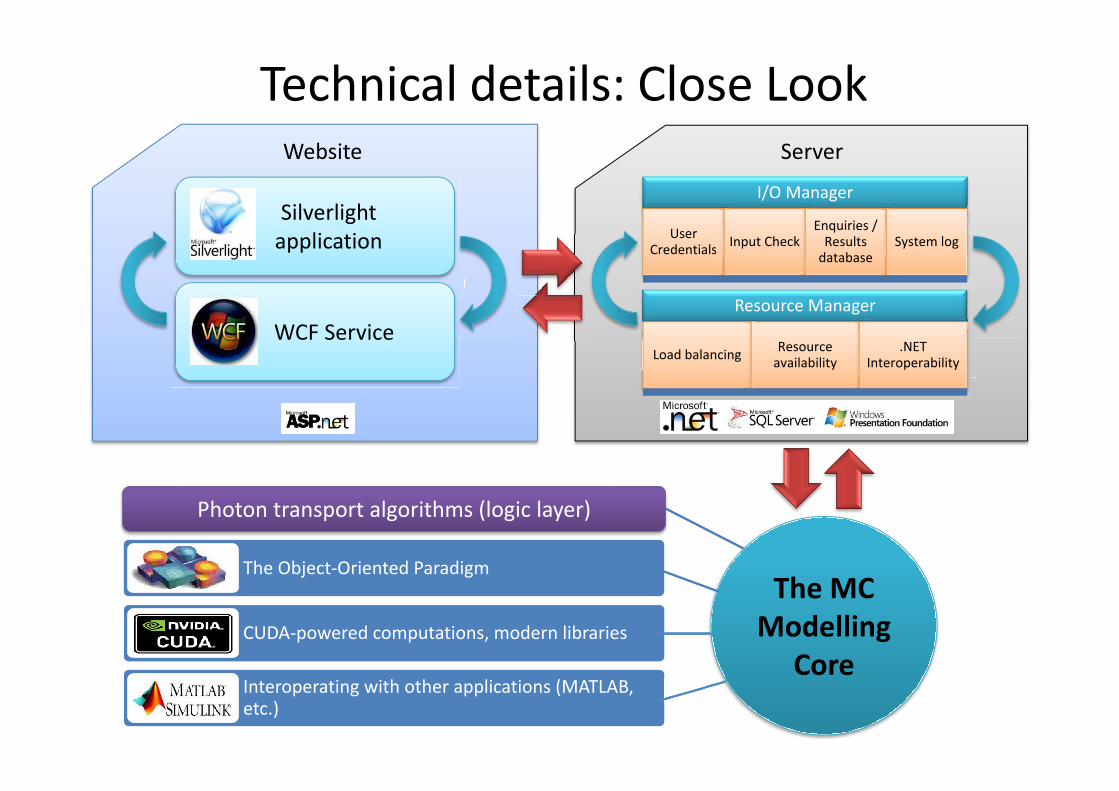
Technical details: Close Look

WCF Service

Silverlight application

Website Server

I/O Manager

User Credentials s Input Check

Enquiries / Results

database System log

Resource Manager

Load balancing Resource availability

.NET Interoperability

Photon transport algorithms (logic layer)

The Object-Oriented Paradigm

CUDA-powered computations, modern libraries

Interoperating with other applications (MATLAB, etc.)

The MC Modelling

Core

Accessing the Tool 1. Open you favourite web browser and type http://biophotonics.otago.ac.nz/ in the

address bar

1. Chose the tab named “Monte Carlo Online” on the top menu to load the Monte Carlo web application.

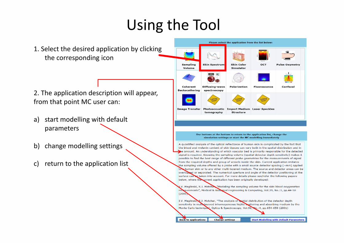
Using the Tool 1. Select the desired application by clicking

the corresponding icon

2. The application description will appear, from that point MC user can: a) start modelling with default

parameters

b) change modelling settings

c) return to the application list

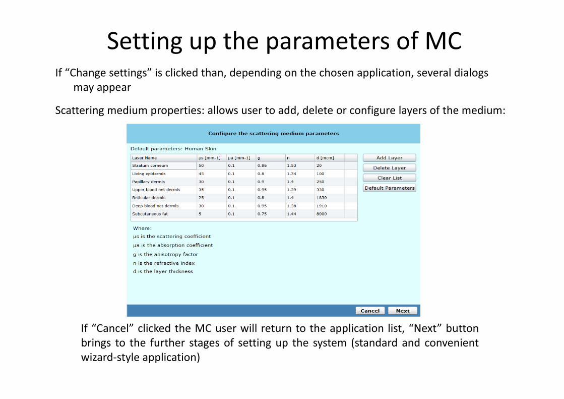
Setting up the parameters of MC If “Change settings” is clicked than, depending on the chosen application, several dialogs

may appear

Scattering medium properties: allows user to add, delete or configure layers of the medium:

If “Cancel” clicked the MC user will return to the application list, “Next” button brings to the further stages of setting up the system (standard and convenient wizard-style application)

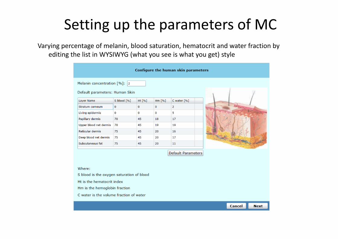
Setting up the parameters of MC Varying percentage of melanin, blood saturation, hematocrit and water fraction by

editing the list in WYSIWYG (what you see is what you get) style

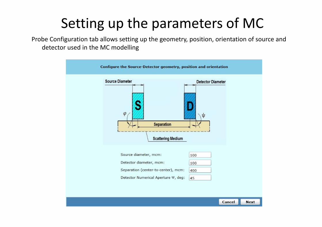
Setting up the parameters of MC Probe Configuration tab allows setting up the geometry, position, orientation of source and

detector used in the MC modelling

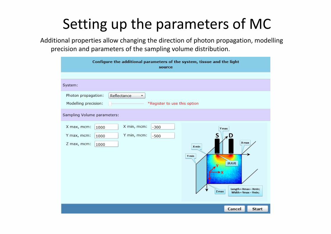
Setting up the parameters of MC Additional properties allow changing the direction of photon propagation, modelling

precision and parameters of the sampling volume distribution.

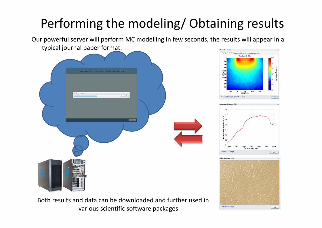
Performing the modeling/ Obtaining results Our powerful server will perform MC modelling in few seconds, the results will appear in a

typical journal paper format.

Both results and data can be downloaded and further used in various scientific software packages

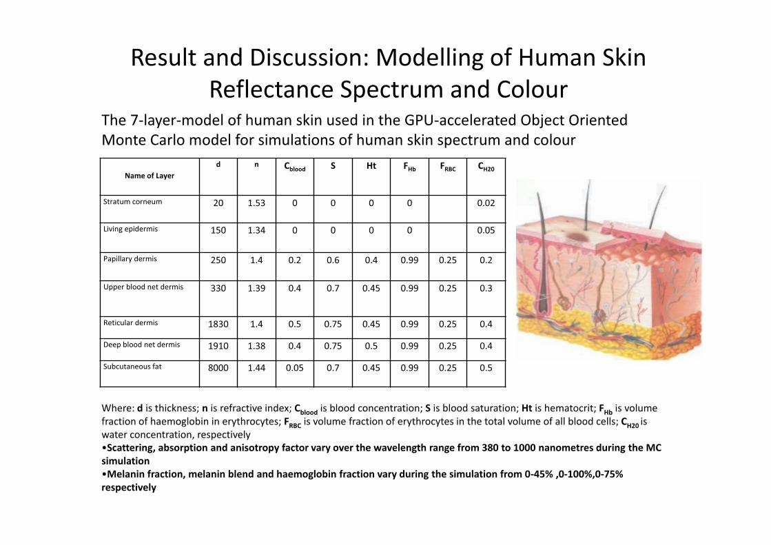
Result and Discussion: Modelling of Human Skin Reflectance Spectrum and Colour

Name of Layer

d n Cblood S Ht FHb FRBC CH20

Stratum corneum 20 1.53 0 0 0 0 0.02

Living epidermis 150 1.34 0 0 0 0 0.05

Papillary dermis 250 1.4 0.2 0.6 0.4 0.99 0.25 0.2

Upper blood net dermis 330 1.39 0.4 0.7 0.45 0.99 0.25 0.3

Reticular dermis 1830 1.4 0.5 0.75 0.45 0.99 0.25 0.4

Deep blood net dermis 1910 1.38 0.4 0.75 0.5 0.99 0.25 0.4

Subcutaneous fat 8000 1.44 0.05 0.7 0.45 0.99 0.25 0.5

Where: d is thickness; n is refractive index; Cblood is blood concentration; S is blood saturation; Ht is hematocrit; FHb is volume fraction of haemoglobin in erythrocytes; FRBC is volume fraction of erythrocytes in the total volume of all blood cells; CH20 is water concentration, respectively •Scattering, absorption and anisotropy factor vary over the wavelength range from 380 to 1000 nanometres during the MC simulation •Melanin fraction, melanin blend and haemoglobin fraction vary during the simulation from 0-45% ,0-100%,0-75% respectively

The 7-layer-model of human skin used in the GPU-accelerated Object Oriented Monte Carlo model for simulations of human skin spectrum and colour

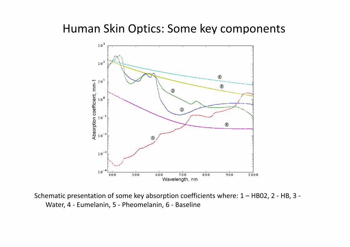
Human Skin Optics: Some key components

Schematic presentation of some key absorption coefficients where: 1 – HB02, 2 - HB, 3 - Water, 4 - Eumelanin, 5 - Pheomelanin, 6 - Baseline

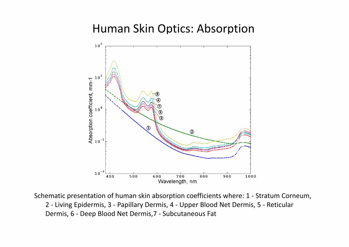
Human Skin Optics: Absorption

Schematic presentation of human skin absorption coefficients where: 1 - Stratum Corneum, 2 - Living Epidermis, 3 - Papillary Dermis, 4 - Upper Blood Net Dermis, 5 - Reticular Dermis, 6 - Deep Blood Net Dermis,7 - Subcutaneous Fat

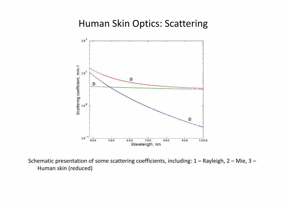
Human Skin Optics: Scattering

Schematic presentation of some scattering coefficients, including: 1 – Rayleigh, 2 – Mie, 3 – Human skin (reduced)

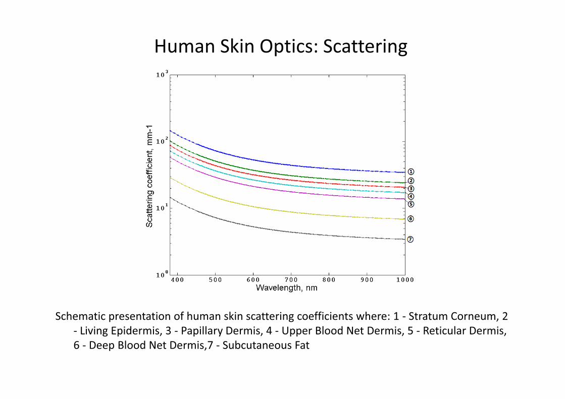
Human Skin Optics: Scattering

Schematic presentation of human skin scattering coefficients where: 1 - Stratum Corneum, 2 - Living Epidermis, 3 - Papillary Dermis, 4 - Upper Blood Net Dermis, 5 - Reticular Dermis, 6 - Deep Blood Net Dermis,7 - Subcutaneous Fat

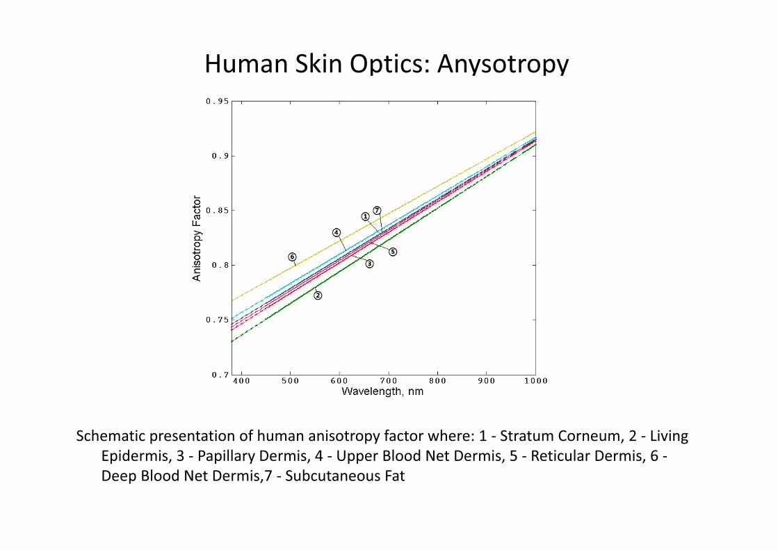
Human Skin Optics: Anysotropy

Schematic presentation of human anisotropy factor where: 1 - Stratum Corneum, 2 - Living Epidermis, 3 - Papillary Dermis, 4 - Upper Blood Net Dermis, 5 - Reticular Dermis, 6 - Deep Blood Net Dermis,7 - Subcutaneous Fat

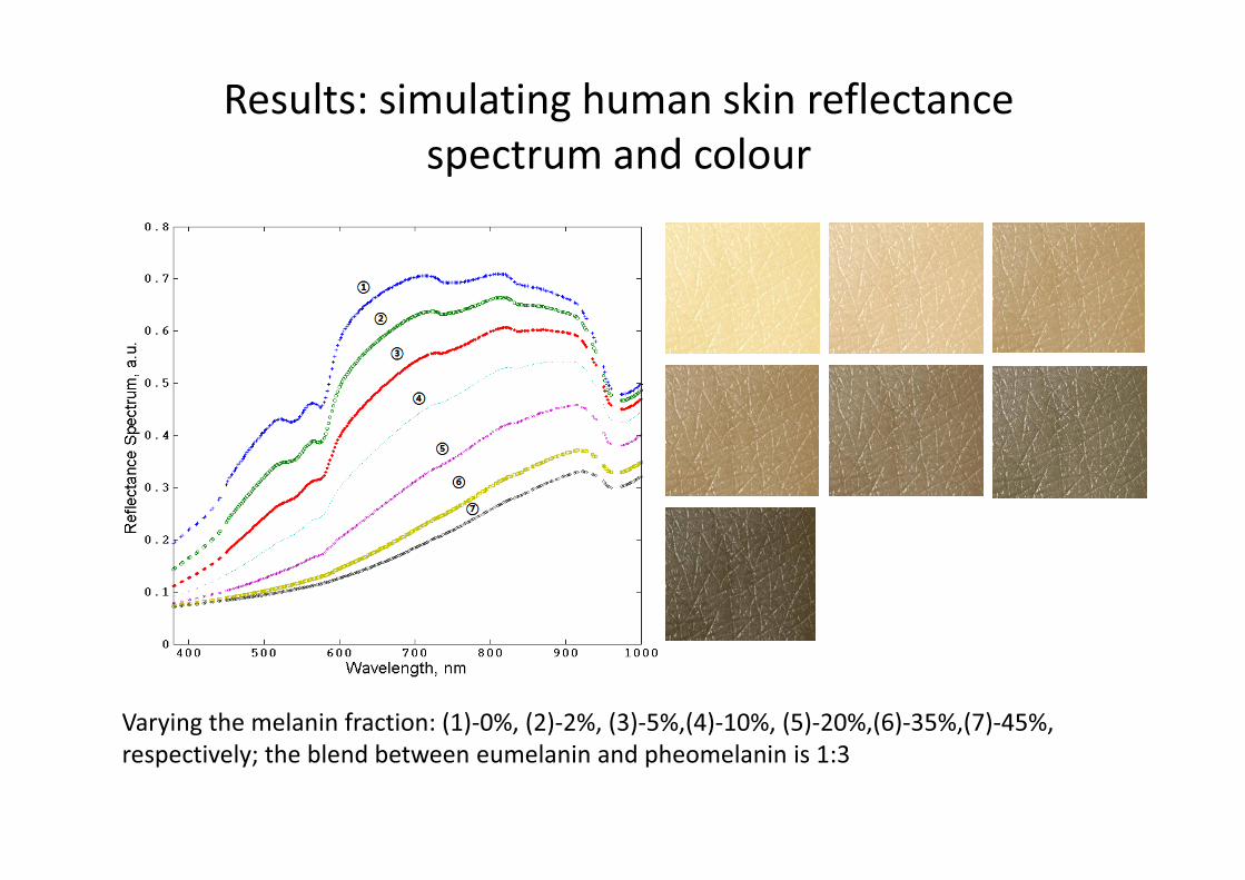
Results: simulating human skin reflectance spectrum and colour

Varying the melanin fraction: (1)-0%, (2)-2%, (3)-5%,(4)-10%, (5)-20%,(6)-35%,(7)-45%, respectively; the blend between eumelanin and pheomelanin is 1:3

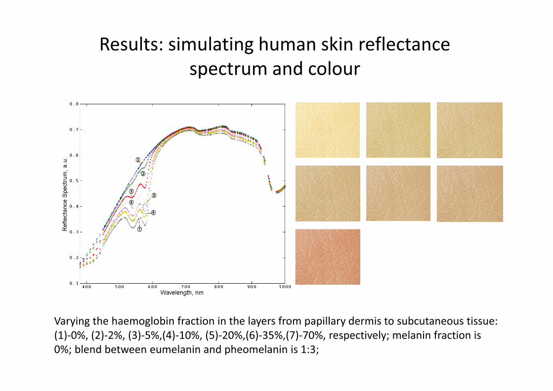
Results: simulating human skin reflectance spectrum and colour

Varying the haemoglobin fraction in the layers from papillary dermis to subcutaneous tissue: (1)-0%, (2)-2%, (3)-5%,(4)-10%, (5)-20%,(6)-35%,(7)-70%, respectively; melanin fraction is 0%; blend between eumelanin and pheomelanin is 1:3;

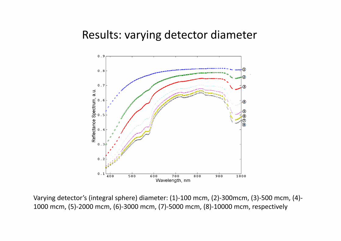
Results: varying detector diameter

Varying detector’s (integral sphere) diameter: (1)-100 mcm, (2)-300mcm, (3)-500 mcm, (4)-1000 mcm, (5)-2000 mcm, (6)-3000 mcm, (7)-5000 mcm, (8)-10000 mcm, respectively

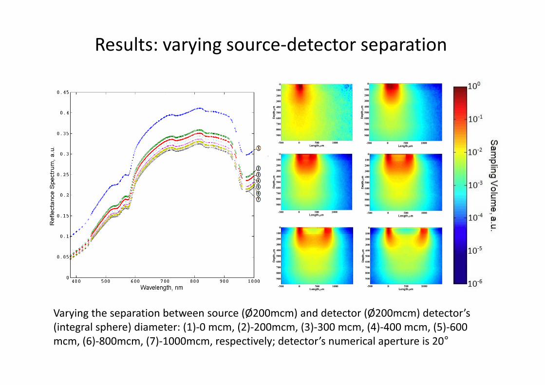
Results: varying source-detector separation

Varying the separation between source (Ø200mcm) and detector (Ø200mcm) detector’s (integral sphere) diameter: (1)-0 mcm, (2)-200mcm, (3)-300 mcm, (4)-400 mcm, (5)-600 mcm, (6)-800mcm, (7)-1000mcm, respectively; detector’s numerical aperture is 20°

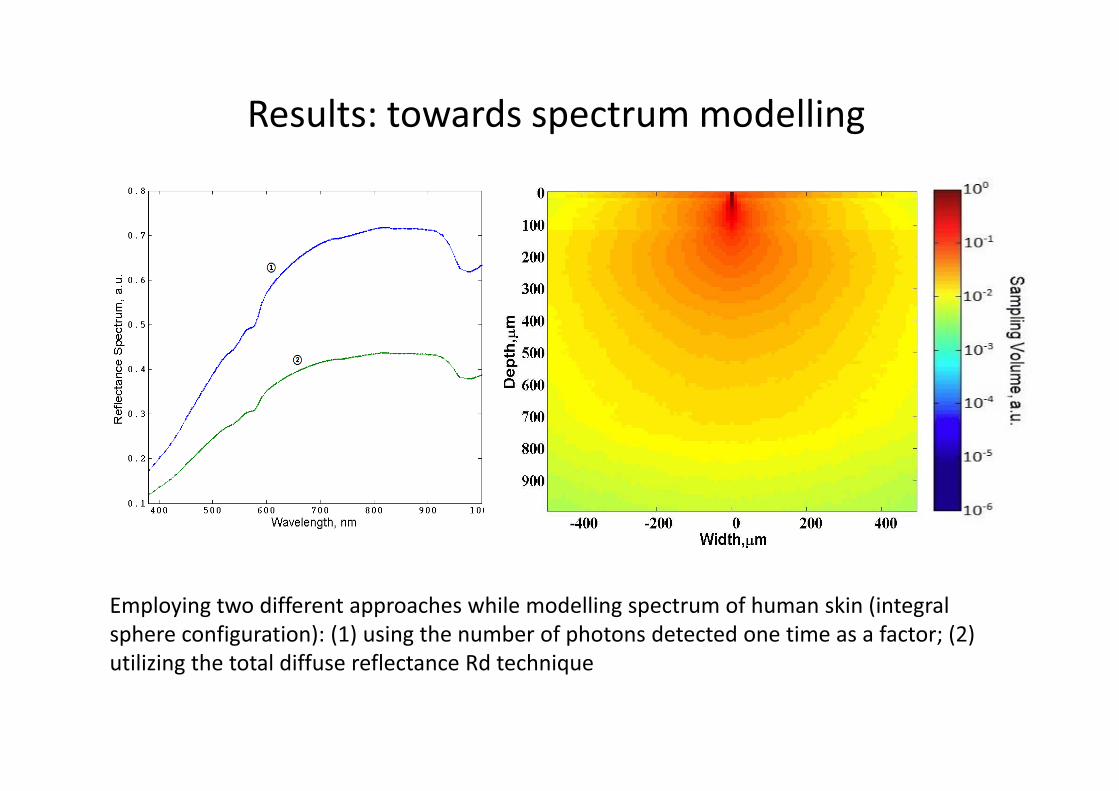
Results: towards spectrum modelling

Employing two different approaches while modelling spectrum of human skin (integral sphere configuration): (1) using the number of photons detected one time as a factor; (2) utilizing the total diffuse reflectance Rd technique

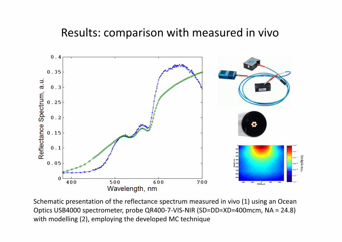
Results: comparison with measured in vivo

Schematic presentation of the reflectance spectrum measured in vivo (1) using an Ocean Optics USB4000 spectrometer, probe QR400-7-VIS-NIR (SD=DD=XD=400mcm, NA = 24.8) with modelling (2), employing the developed MC technique

Acknowledgements

The Royal Society, UK EPSRC & BBSRC, UK

The Royal Academy of Engineering, UK Wellcome Trust, UK

NATO, European Commission, EU LaserLab Europe

CRDF, USA Russian Ministry of Science and Technology, Russia

RFFI, Russia British Council, UK